Multiple imputation of discrete and continuous data by ... by FCS - SMMR 2007.pdf · Multiple imputation of discrete and continuous data by fully conditional speciﬁcation ... 2.2

Statistical Methods in Medical Research 2007; 16: 219–242

Multiple imputation of discrete and continuousdata by fully conditional specification

Stef van Buuren TNO Quality of Life, Leiden, The Netherlands and University of Utrecht,The Netherlands

The goal ofmultiple imputation is to provide valid inferences for statistical estimates from incomplete data.To achieve that goal, imputed values should preserve the structure in the data, as well as the uncertaintyabout this structure, and include any knowledge about the process that generated the missing data. Twoapproaches for imputing multivariate data exist: joint modeling (JM) and fully conditional specification(FCS). JM is based on parametric statistical theory, and leads to imputation procedures whose statisticalproperties are known. JM is theoretically sound, but the jointmodelmay lack flexibility needed to representtypical data features, potentially leading to bias. FCS is a semi-parametric and flexible alternative thatspecifies the multivariate model by a series of conditional models, one for each incomplete variable. FCSprovides tremendous flexibility and is easy to apply, but its statistical properties are difficult to establish.Simulation work shows that FCS behaves very well in the cases studied. The present paper reviews andcompares the approaches. JM and FCS were applied to pubertal development data of 3801 Dutch girlsthat had missing data on menarche (two categories), breast development (five categories) and pubic hairdevelopment (six stages). Imputations for these data were created under twomodels: a multivariate normalmodel with rounding and a conditionally specified discrete model. The JM approach introduced biasesin the reference curves, whereas FCS did not. The paper concludes that FCS is a useful and easily appliedflexible alternative to JM when no convenient and realistic joint distribution can be specified.

1 Introduction

Multiple imputation (MI) is a general statistical method for the analysis of incompletedata sets.1,2 A statistical analysis using multiple imputation typically comprises threemajor steps. The first step involves specifying and generating plausible synthetic datavalues, called imputations, for the missing values in the data. This step results in anumber of complete data sets (m) in which the missing data are replaced by randomdraws from a distribution of plausible values. The number of imputations, m, typicallyvaries between 3 and 10. The second step consists of analyzing each imputed data setby a statistical method that will estimate the quantities of scientific interest. This stepresults in m analyses (instead of one), which will differ only because the imputationsdiffer. The third step pools the m estimates into one estimate, thereby combining thevariation within and across them imputed data sets. Under fairly liberal conditions, thisstep results in statistically valid estimates that translate the uncertainty caused by themissing data into the width of the confidence interval.

Address for correspondence: Stef van Buuren, TNO Quality of Life, Leiden, The Netherlands. E-mail:[email protected]

© 2007 SAGE Publications 10.1177/0962280206074463

© 2007 SAGE Publications. All rights reserved. Not for commercial use or unauthorized distribution. at SWETS WISE ONLINE CONTENT on July 31, 2007 http://smm.sagepub.comDownloaded from

220 S van Buuren

MI is a highly modular statistical method in the sense that the steps can be executedseparately, and with relatively limited interaction between the steps. The major rule thatconnects steps 1 and 2 is that every relation to be studied in the step 2 should, in someway, be included into the specification of the plausible values for the missing data instep 1. Failure to do so may bias the estimates towards the null, the amount of whichdepends on the amount of missing data and the strength of the relationship of interest.It should be pointed out however that for such failures to occur the relations have to bequite strong and the amount of missing information has to be quite high.3

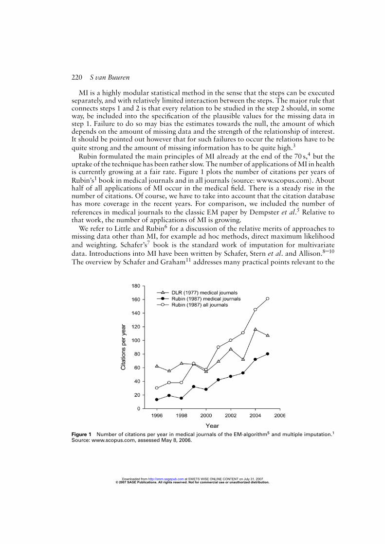
Rubin formulated the main principles of MI already at the end of the 70 s,4 but theuptake of the technique has been rather slow. The number of applications ofMI in healthis currently growing at a fair rate. Figure 1 plots the number of citations per years ofRubin’s1 book in medical journals and in all journals (source: www.scopus.com). Abouthalf of all applications of MI occur in the medical field. There is a steady rise in thenumber of citations. Of course, we have to take into account that the citation databasehas more coverage in the recent years. For comparison, we included the number ofreferences in medical journals to the classic EM paper by Dempster et al.5 Relative tothat work, the number of applications of MI is growing.We refer to Little and Rubin6 for a discussion of the relative merits of approaches to

missing data other than MI, for example ad hoc methods, direct maximum likelihoodand weighting. Schafer’s7 book is the standard work of imputation for multivariatedata. Introductions into MI have been written by Schafer, Stern et al. and Allison.8–10

The overview by Schafer and Graham11 addresses many practical points relevant to the

Figure 1 Number of citations per year in medical journals of the EM-algorithm5 and multiple imputation.1

Source: www.scopus.com, assessed May 8, 2006.


Multiple imputation of discrete and continuous data 221

application of MI. Overviews of MI in health have been written by Rubin and Schenkerand Barnard and Meng.12,13 Evaluations of MI and comparative reviews have appearedin various medical fields: epidemiology,14–16 psychiatric and developmental research,17

nursing research,18–21 public health,22–24 cost and outcomes research,25–27 quality oflife,(28) and physical activity,29,30 educational research,31,32 and chemometrics.33 Moremethodologically oriented comparative reviews have appeared on multilevel models,34

structural equation modeling,35,36 methods for longitudinal data,37,38 attrition prob-lems in longitudinal data,39,40 drop out in clinical trials,41–46 and meta-analysis.47

Ibrahim et al.48 provide a comparative review of various advanced missing data meth-ods. Schafer49 comparesBayesianMImethodswithdirectmaximum likelihoodmethods.Taken together, these references provide abundant evidence on the value and vitality ofMI in health research.The present paper deals with the question how to create multiple imputations for

multivariate data. The paper provides an overview of methods for generating multipleimputations, starting from basic methods where the missing values are confined to onevariable, and continuing to more advanced methods for dealing with general patternsof missing values in multivariate data of various types, including mixes of categoricaland continuous data. We distinguish between approaches based on both joint modeling(JM) and fully conditional specification (FCS). An application on pubertal data fromthe Fourth Dutch Growth Study illustrates the principles.

2 Method

2.1 NotationLet Yj be one of k incomplete random variables ( j = 1, . . . , k) and let Y =

(Y1, . . . ,Yk). The observed andmissing parts ofYj are denoted byYobsj andYmisj , respec-

tively, so Yobs = (Yobs1 , . . . ,Yobsk

) and Ymis = (Ymis1 , . . . ,Ymisk

) stand for the observedand missing data in Y. Let Y−j = (Y1, . . . ,Yj−1,Yj+1, . . . ,Yk) denote the collec-tion of the k − 1 variables in Y except Yj. Let Rj be the response indicator of Yj,with Rj = 1 if Yj is observed and Rj = 0 if Yj is missing. Let R = (R1, . . . ,Rk) andR−j = (R1, . . . ,Rj−1,Rj+1, . . . ,Rk). LetX = (X1, . . . ,Xl) be a set of l complete covari-ates on the same subjects. In order to avoid distracting complexities, we assume that theobservations in Y,X and R correspond to a simple random sample from the populationof interest.

2.2 Imputation modelsRubin1 (Ch. 5) distinguished three tasks for creating imputations under an explicit

model: the modeling task the imputation task and the estimation task. The model-ing task is to provide a specification for the hypothetical joint distribution P(Y,X,R)of all data. The imputation task sets out to derive the posterior predictive distri-

bution P(Ymis|Yobs,X,R) of the missing values Ymis given the observed data. Theestimating task consists of calculating the posterior distribution of the parameters of


222 S van Buuren

this distribution, so that random draws can be made from it. According to Rubin’sframework, the imputations follow from the specification of the joint model P(Y,X,R).In practice, it is often difficult to specify a realistic joint model P(Y,X,R). Model

P(Y,X,R) embraces both the model for generating the imputations and the scientifi-cally interesting model for which the data were sampled in the first place. This dual roleof P(Y,X,R) puts a heavy burden on its specification. Several classes of joint modelshave been proposed. Schafer developed joint models (JM) for imputation under the mul-tivariate normal (MVN), the log-linear and the general location model.7 The methodsare theoretically elegant, but they often lack flexibility to account for important fea-tures of the data. For example, if the data contain derived variables (e.g., sum scores,transformations, indices) onewould like the imputation procedure to ensure consistencybetween the constituent parts.Multivariate imputation according to a joint model couldalso create impossible combinations like ‘pregnant fathers’, which are better avoided inthe imputed data. The rows or columns could have a meaningful order, for example, asin longitudinal data. Real data often consist of amix of different scale types (e.g., binary,unordered, ordered, continuous). Also, the relation between Yj and predictors Y−j canbe complex, for example, nonlinear or be subject to censoring or rounding or containinteractions that are important. Enforcing parametric joint models P(Y,X,R) on thedata potentially discards interesting features in the data that we may wish to investigateandmay thus severely limit the class of scientific models that may be legitimately appliedto the imputed data.Fortunately, imputations of high quality can be generated without an explicit specifi-

cation of P(Y,X,R). An imputation model P(Ymis|X,Yobs,R) describes how syntheticvalues for Ymis = (Ymis1 , . . . ,Ymis

k) are generated. The imputation model can be an

explicit probability model, or an implicit model, like hot-deck (Little and Rubin, 2002,p. 67). In principle, the imputation model can correspond to any method to augmentthe data, as long as it yields imputations that are proper in the sense of Rubin (1987,p. 119). A procedure is proper if particular conditions hold for the complete-data statis-tics and the within and between imputation variances in the casem = ∞. An importantrequirement for a procedure to be proper is that the variability of the parameters ofthe imputation model should be included into the generated imputations, a propertythat Schafer7 calls ‘Bayesianly proper’. It is actually difficult to demonstrate proper-ness analytically in a given case (Schafer, 1997, p. 145). Brand et al.50 for a validationstrategy based on simulation to assess various aspects of properness. Note that the

imputation model P(Ymis|X,Yobs,R) need not make an explicit reference to a specifica-tion for P(Y,X,R) and that it does not automatically follow from the joint distributionP(Y,X,R). Imputation models bypass the need to specify P(Y,X,R), though their usecreates new responsibilities for substantiating its correctness for a given statistical anal-

ysis. Instead of specifying P(Y,X,R), using models P(Ymis|X,Yobs,R) is a separatemodeling activity that comes with its own goals and rules.3,49,51–53

This paper is based on the idea that we may bypass the (joint) modelingtask, and directly specify a sensible model for creating multivariate imputa-

tions P(Ymis|X,Yobs,R). A convenient way of doing that is to generate imputa-tions in multivariate data variable-by-variable by specifying a conditional modelP(Ymisj |X,Y−j,R) for each Yj, j = 1, . . . , k.



2.3 IgnorabilityLet us first look at the role of R within the imputation model. The imputation model

for variable j, P(Ymisj |X,Y−j,R), exploits relations between and within Y, X and R. Let

us for the moment assume that k = 1, so that there is only one Y with missing data.In that case, the information about Y that is present in X and R is summarized bythe conditional distribution P(Y|X,R). Cases with missing Y, that is, with R = 0, donot provide any information about P(Y|X,R), and so in actual data analysis it is onlypossible to fit models for P(Y|X,R = 1). It is, however, the distribution P(Y|X,R = 0)that we need to draw imputations from, and the central problem is how to specify thatdistribution. The conventional procedure is to equate P(Y|X,R = 0) = P(Y|X,R = 1),which corresponds to the assumption that the response mechanism is ignorable (Rubin,1987, pp. 51–53).The assumption of ignorability is often sensible in practice and generally provides

a natural starting point. If, on the other hand, the assumption is not reasonable (e.g.,when data are censored), wemay use other forms for P(Y|X,R = 0). The fact thatR = 0allows for the possibility that P(Y|X,R = 1) 6= P(Y|X,R = 0) (Rubin, 1987, p. 205). Bydefinition, the specification of P(Y|X,R = 0) needs assumptions external to the data. Aslong as the imputations reflect the correct amount of uncertainty about the values thatare missing, there is nothing in the theory of MI that prevents appropriate inferencesunder P(Y|X,R = 0). MI will also work for nonignorable response mechanisms.

Example: Suppose that a growth study measures body weight in kg (Y) and gender(X1: 1 = boy, 0 = girl) of 15-year old children, and that some of the body weights aremissing.We canmodel theweight distribution for boys and girls separately for thosewithobserved weights, that is, P(Y|X1 = 1,R = 1) and P(Y|X1 = 0,R = 1). If we assumethat the response mechanism is ignorable, then imputations for a boy’s weight can bedrawn from P(Y|X1 = 1,R = 0) = P(Y|X1 = 1,R = 1). The same can be done for girls.This procedure leads to correct inferences on the combined sample of boys and girls, evenif boys have substantiallymoremissing values, or if the bodyweights of the boys and girlsare very different. The procedure is however not appropriate if, within the group of boysor the girls, the occurrence of the missing data is related to body weight. For example,someof the heavier childrenmaynotwant to beweighed, resulting inmoremissing valuesfor themore obese. It will be clear that assuming P(Y|X1,R = 0) = P(Y|X1,R = 1)willthen underestimate the prevalence of overweight and obesity. In this case, it may be morerealistic to specify P(Y|X1,R = 0) such that imputation accounts for the excess bodyweights in the children that were not weighed. There are many ways to do that. In allthese cases the response mechanism will be nonignorable.The assumption of ignorability is essentially the belief on the part of the user that the

available data are sufficient to correct for the effects of the missing data. The assump-tion cannot be tested on the data itself, but it can be checked against suitable externalvalidation data. There are two main strategies that we may pursue if the response mech-anism is not ignorable. The first is to expand the data and assume ignorability on theexpanded data. In the above example, fat children may simply not want anybody toknow their weight, but perhaps have no objection if their waist circumference (X2) ismeasured.The ignorability assumptionP(Y|X,R = 0) = P(Y|X,R = 1) is less stringentforX = (X1,X2) than forX = (X1), and hence more realistic. The second strategy is to


224 S van Buuren

formulate P(Y|X,R = 0) different from P(Y|X,R = 1), describing which body weightswould have beenobserved if they hadbeenmeasured.Candidates for suchmodels includethe pattern mixture model and the selection model, though application of such modelsrequires untestable a priori assumptions beyond the data (Little andRubin, 2002, Ch. 15;Schafer, 1997, p. 28).6,7

We may disregard R in the imputation model if we are prepared to make the assump-tion of ignorability. If this is not realistic, then we can pursue one of the two strategiesoutlined above. Of course, any such methods need to be explained and justified as partof the statistical analysis.

3 Univariate and monotone imputation

For both theoretical and practical reasons, it is useful to distinguish between monotoneand nonmonotone missing data patterns. A pattern is monotone if the variables can beordered such that, for each person, all earlier variables are observed if the later variable isobserved. Monotone patterns often occur as a result of dropout in a longitudinal study.It is often useful to sort variables and cases to approach a monotone pattern. Figure 2depicts various monotone and nonmonotone missing data patterns.

3.1 Univariate methodsAn important special case of a monotone missing data pattern occurs when k = 1. In

that case, there is only one Y that needs to be imputed and the remaining data X are allcomplete. Table 1 contains an overview of various methods that have been proposed forgenerating multiple imputations for univariate data. Many methods are variations onthe linear regression method proposed by Rubin (1987, p. 166).1

3.2 Monotone patternsImputations for multivariate missing data can be imputed by a sequence of univari-

ate methods if the missing data pattern is monotone-distinct.1 Suppose that variablesY1, . . . ,Yk are ordered in a monotone pattern such that for j = 1, . . . , k − 1, all caseswith missing data in Yj also have missing data in Y>j. If, in addition, the parametersφ1, . . . ,φk of the imputation models are a priori independent, that is, if they factor intoindependent marginal priors, we can draw a set of multivariate imputations using thefollowing sequence of univariate imputation models

P(Ymis1 |X,φ1)

P(Ymis2 |X,Y∗1,φ2)

. . .

P(Ymisk |X,Y∗1, . . . ,Y

∗k−1,φk)

where notation Y∗j stands for the jth imputed variable. The sequence can be replicated

m times from different starting points to obtain multiple imputations. Univariate meth-ods such as listed in Table 1 can be used as building blocks. There is no need to iterate.



Figure 2 Four types of missing data patterns in multivariate data. The grey parts represent observed data,whereas the empty parts indicate missing data.

Since this procedure is convenient, it is often useful to identify whether the data can beordered to a (nearly) monotone pattern. It is beneficial to impute to entries that destroythe monotone pattern first and then apply the above method.7,77,78 It may however beimpossible to reorder variables into a monotone pattern. In that case, we need a trulymultivariate imputation method.


226 S van Buuren

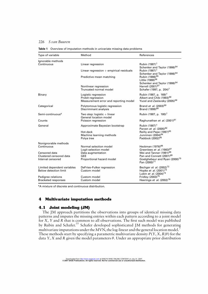
Table 1 Overview of imputation methods in univariate missing data problems

Type of variable Method References

Ignorable methodsContinuous Linear regression Rubin (1987)1

Schenker and Taylor (1986)54

Linear regression + empirical residuals Rubin (1987)1


Predictive mean matching Rubin (1986)55

Little (1988)56


Nonlinear regression Harrell (2001)57

Truncated normal model Schafer (1997, p. 204)7

Binary Logistic regression Rubin (1987, p. 169)1

Probit regression Albert and Chib (1993)58

Measurement error and reporting model Yucel and Zaslavsky (2005)59

Categorical Polytomous logistic regression Brand et al. (2003)50

Discriminant analysis Brand (1999)60

Semi-continuousa Two step: logistic + linear Rubin (1987, p. 180)1

General location modelCounts Poisson regression Raghunathan et al. (2001)61

General Approximate Bayesian bootstrap Rubin (1987)1

Parzen et al. (2005)62

Hot-deck Reilly and Pepe (1997)63

Machine learning methods Junninen (2004)64

Polya tree Paddock (2002)65

Nonignorable methodsContinuous Normal selection model Heckman (1976)66

Logit selection model Greenlees et al. (1983)67

Censored data Data augmentation Wei and Tanner (1991)68

Clustered censored data GEE Pan and Connett (2001)69

Interval censored Proportional hazard model Goetghebeur and Ryan (2000)70

Pan (2000)71

Limited dependent variables DeFries–Fulker regression Bechger et al. (2002)72

Below detection limit Custom model Hopke et al. (2001)73

Lubin et al. (2004)74

Pedigree relations Custom model Fridley (2003)75

Bracketed responses Custom model Heeringa et al. (2002)76

aA mixture of discrete and continuous distribution.

4 Multivariate imputation methods

4.1 Joint modeling (JM)The JM approach partitions the observations into groups of identical missing data

patterns and imputes the missing entries within each pattern according to a joint modelfor X, Y and R that is common to all observations. The first such model was publishedby Rubin and Schafer.77 Schafer developed sophisticated JM methods for generatingmultivariate imputationsunder theMVN, the log-linear and the general locationmodel.7

These methods start by specifying a parametric multivariate density P(Y,X,R|θ) for thedata Y,X and R given the model parameters θ . Under an appropriate prior distribution



for θ , it is possible to derive the appropriate submodel for each missing data pattern,fromwhich imputations are drawn, usually under the assumptionof an ignorablemissingdata mechanism. These methods are available as tools in S-Plus 7.0 and SAS V8.2 andare widely applied.

4.2 Fully conditional specification (FCS)The FCS approach is to impute the data on a variable-by-variable basis by specifying

an imputationmodel per variable. FCS is an attempt to define P(Y,X,R|θ) by specifyinga conditional density P(Yj|X,Y−j,R, θj) for eachYj. This density is used to imputeYmisj

givenX, Y−j and R. Starting from simple guessed values, imputation under FCS is doneby iterating over all conditionally specified imputationmodels.Methods listed in Table 1may act as building blocks. One iteration consists of one cycle through allYj. If the jointdistribution defined by the specified conditional distributions exists, then this process isa Gibbs sampler.FCS has some practical advantages over JM. FCS allows tremendous flexibility in

creating multivariate models. One can easily specify models that are outside any knownstandardmultivariate density P(X,Y,R|θ). FCS can use specialized imputationmethodsthat are difficult to formulate as a part of amultivariate densityP(X,Y,R|θ). Imputationmethods that preserve unique features in the data, for example, bounds, skip patterns,interactions, bracketed responses and so on can be incorporated. It is straightforward tomaintain constraints between different variables in order to avoid logical inconsistenciesin the imputed data. It would be rather difficult to formulate such constraints in terms ofthe multivariate density P(X,Y,R|θ). Each conditional density has to be specified sepa-rately, so some modeling effort may be required on the part of the user. Computationalshortcuts like the sweep operator6 cannot be used anymore, so the calculations couldbe more intensive than for JM.Despite the lack of a satisfactory theory, FCS seems to work quite well in many

applications. A number of simulation studies provide evidence that FCS generally yieldsestimates that are unbiased and that possess appropriate coverage, at least in the varietyof cases investigated.50,60,61,79,80

The basic idea of FCS is already quite old and has been proposed using avariety of names: stochastic relaxation,81 variable-by-variable imputation,60 regres-sion switching,52 sequential regressions,61 ordered pseudo-Gibbs sampler,82 partiallyincompatible MCMC,78 iterated univariate imputation,83 chained equations84 andFCS.79

4.3 Relations between FCS and JMFCS is related to JM in some cases. If P(X,Y) has an MVN model distribution, then

all conditional densities are linear regressions with a constant normal error variance.So, if P(X,Y) is MVN then P(Yj|X,Y−j) follows a linear regression model. The reverseis also true: if the imputation models P(Yj|X,Y−j) are all linear with constant normalerror variance, then the joint distribution will beMVN.We refer to Arnold et al. (p. 186)for a description of the precise conditions.85 Thus, imputation by FCS using all linear


228 S van Buuren

regressions is identical to imputation under theMVNmodel. In that case, the algorithmis a real Gibbs sampler, and convergence is guaranteed.Another special case occurs for binary variables with only two-way interactions in

the log-linear model. For example, in the case k = 3, suppose that Y1, . . . ,Y3 are mod-eled by the log-linear model that has the three-way interaction term set to zero. Itis known that the corresponding conditional distribution P(Y1|Y2,Y3) is the logisticregression model log(P(Y1)/1− P(Y1)) = β0 + β2Y2 + β3Y3.

86 Analogous definitionsexist for P(Y2|Y1,Y3) andP(Y3|Y1,Y2). Thismeans that ifwe use logistic regressions forY1,Y2 andY3, we are effectively imputing under multivariate ‘no three-way interaction’log-linear model. In this case, the method is also a Gibbs sampler.

5 Issues in FCS

5.1 CompatibilityIt is quite easy to specify a set of conditional distributions for which no multi-

variate density exists. An example is the combination of Y2|Y1 ∼ N(α2 + β1Y1, σ21 )

with Y1|Y2 ∼ N(α1 + β2 log(Y2), σ22 ), but the issues involved are actually quite subtle.

Incompatibility is a theoretical weakness of FCS, because it is not known to which mul-tivariate distribution the algorithm converges. The limiting distribution to which thealgorithm converges may depend on the order of the univariate imputation steps, whichmay or may not be desirable in a given context. Consequently, assessing convergenceis a somewhat ambiguous activity. The issue is known as incompatibility of condition-als, and has been studied by various authors.85,87–89 Gelman and Speed89 showed thatthe joint distribution for Y1, . . . ,Y3, if it exists, is uniquely specified by the follow-ing set of three conditionals: P(Y1|Y2,Y3), P(Y2|Y3) and P(Y3|Y1). Imputation underFCS typically specifies general forms for P(Y1|Y2,Y3), P(Y2|Y1,Y3) and P(Y3|Y1,Y2)and estimates the free parameters for these conditionals from the data. Typically, thenumber of parameters in imputation is much larger than needed to uniquely determineP(Y1,Y2,Y3).Notmuch is known about the consequences of incompatibility on the quality of impu-

tations. Van Buuren et al.79 report some simulations under some strongly incompatiblemodels and observe that the adverse effects on the estimates afterMIwere onlyminimal.More work is needed to verify such claims in more general and more realistic settings.In cases where the multivariate density is of genuine scientific interest, incompatibility

clearly represents a problem because the data cannot be represented by a formal model.So given the dual role of P(Y,X,R) for both analysis and imputation (Section 2.2),incompatibility is clearly undesirable within a JM context. In imputation however, theobjective is to augment the data and preserve the relations in the data. In that case,the joint distribution is more like a nuisance factor that has no intrinsic value. Gelmanremarked: ‘One may argue that having a joint distribution in the imputation is lessimportant than incorporating information from other variables and unique features ofthe dataset (e.g., zero/nonzero features in income components, bounds, skip patterns,nonlinearity, interactions).83



FCS is highly important from a practical point of view because it adapts so well to thedata. FCS is guaranteed to work if the conditionals are compatible and some evidenceis available on the robustness of FCS against incompatibility.

5.2 Assessment of convergenceWhenm sampling streams are calculated in parallel, monitoring convergence is done

by plotting the draws in each stream against time for a set of selected parameters. Thepattern should be inspected for any absence of trend, and convergence can be assessedby test statistics that combine within and between variation.90

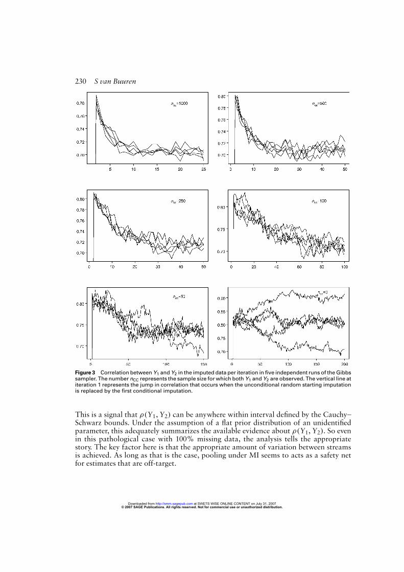
In practice, we have seen many cases where essentially nothing happened after thefirst few iterations. In those applications, we have therefore set the main number ofFCS iterations quite low, usually somewhere between 5 and 20 iterations. This num-ber is much lower than in other applications of MCMC methods, which often requirethousands of iterations. There are exceptions however. In order to demonstrate this,consider a small simulation experiment with three variables: one complete covariate Xand two incomplete variables Y1 and Y2. The data consisted of 10 000 draws from theMVN distribution with correlations ρ(X,Y1) = ρ(X,Y2) = 0.9 and ρ(Y1,Y2) = 0.7.The number of complete cases (CC) was varied as nCC = (1000, 500, 250, 100, 50, 0).Missing data were randomly created in two patterns (X, NA,Y2) and (X,Y1, NA), bothof size (10 000− nCC)/2, where symbol ‘NA’ stands for themissing entry. Amissing datapattern like this may result in statistical matching problems, whereY1 andY2 are jointlyobserved only for a subset of nCC cases.

55 The difficulty in this particular problem isthat the correlation ρ(Y1,Y2) under conditional independence of Y1 and Y2 given X isequal to 0.9× 0.9 = 0.81, whereas the true value equals 0.7. We used compatible lin-ear regressions Y1 = β1,0 + β1,2Y2 + β1,3X + ε1 and Y2 = β2,0 + β2,1Y1 + β2,3X + ε2to impute Y1 and Y2, so the algorithm is a Gibbs sampler.Figure 3 shows the development of ρ(Y1,Y2) calculated on the completed data after

every iteration of the Gibbs sampler. At iteration 1, ρ(Y1,Y2) is around 0.40 (not shownin the figure), due to the random starting imputations. At iteration 2, ρ(Y1,Y2) jumps tothe value expected givenX only. After iteration 2, the influence of the nCC pairswith bothY1 andY2 observed percolates into the imputations, so that the chains slowly move intothe direction of the population value of 0.7. The speed of convergence heavily depends onthe value of nCC. If nCC = 1000, that is, if 90% of the record are incomplete, the streamsare essentially flat after about 15 iterations. If nCC = 0, the correlation ρ(Y1,Y2) isunidentified because there is no information about it in the data. The streams do notconverge at all, and wander widely within the Cauchy–Schwarz bounds (0.6–1.0 here).The Cauchy–Schwarz inequality provides the upper and lower bounds for a correlationρ(Y1,Y2) in a positive semi-definite correlation matrix. The lesson from this simulationis that we should be quite careful about convergence in missing data patterns that resultsfrom, for example, statistical matching problems.One final note of interest in this analysis is the following. In the case nCC = 0we could

stop at iteration 200 and take the imputations from there. From a Bayesian perspective,this still would yield a valid inference on ρ(Y1,Y2). The mean value of ρ(Y1,Y2) wasequal to 0.812, and its standard error after pooling was large for this sample size: 0.087.


230 S van Buuren

Figure 3 Correlation between Y1 and Y2 in the imputed data per iteration in five independent runs of the Gibbssampler. The number nCC represents the sample size for which both Y1 and Y2 are observed. The vertical line atiteration 1 represents the jump in correlation that occurs when the unconditional random starting imputationis replaced by the first conditional imputation.

This is a signal that ρ(Y1,Y2) can be anywhere within interval defined by the Cauchy–Schwarz bounds. Under the assumption of a flat prior distribution of an unidentifiedparameter, this adequately summarizes the available evidence about ρ(Y1,Y2). So evenin this pathological case with 100% missing data, the analysis tells the appropriatestory. The key factor here is that the appropriate amount of variation between streamsis achieved. As long as that is the case, pooling under MI seems to acts as a safety netfor estimates that are off-target.



Of course, it never hurts to do a couple of extra iterations or to start more streams,but good results can often be obtained with a small number of iterations.

5.3 SoftwareSystems for creating multiple imputations by FCS include FRITZ,81 IVEWARE

in SAS,61 HERMES missing data engine,60 MICE in S-Plus and R,84 and ICE, animplementation of MICE to Stata.91–92

6 Fourth Dutch Growth Study

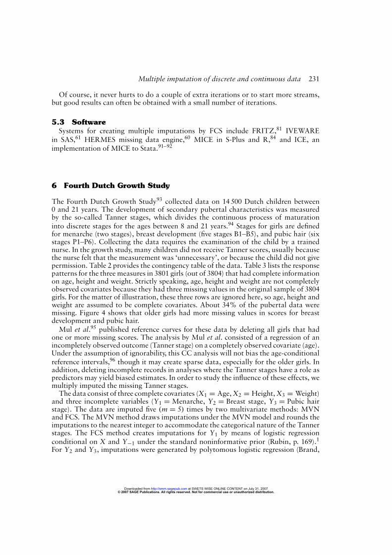
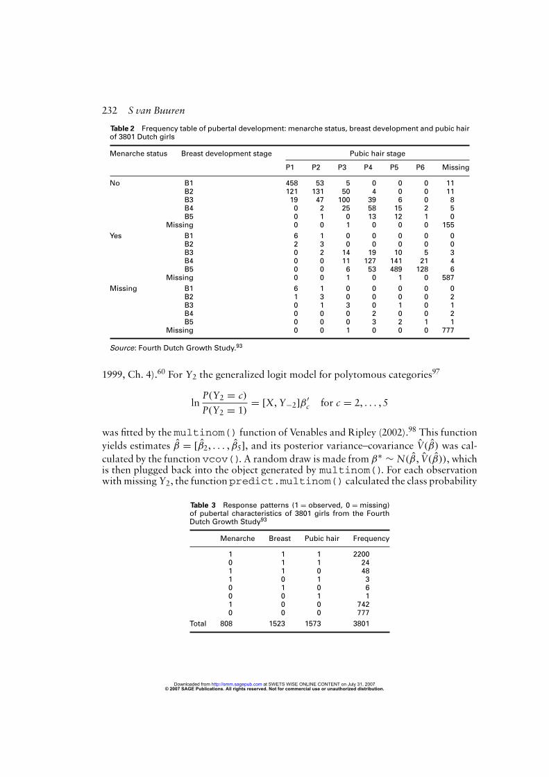
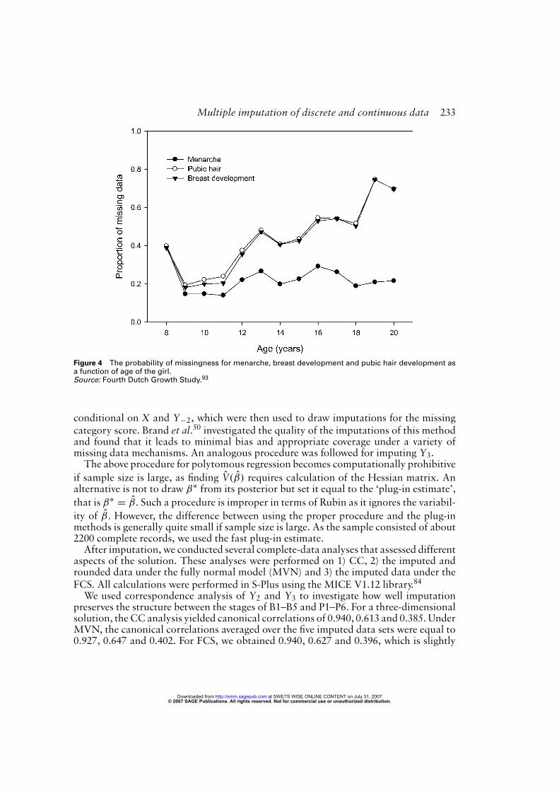
The Fourth Dutch Growth Study93 collected data on 14 500 Dutch children between0 and 21 years. The development of secondary pubertal characteristics was measuredby the so-called Tanner stages, which divides the continuous process of maturationinto discrete stages for the ages between 8 and 21 years.94 Stages for girls are definedfor menarche (two stages), breast development (five stages B1–B5), and pubic hair (sixstages P1–P6). Collecting the data requires the examination of the child by a trainednurse. In the growth study, many children did not receive Tanner scores, usually becausethe nurse felt that the measurement was ‘unnecessary’, or because the child did not givepermission. Table 2 provides the contingency table of the data. Table 3 lists the responsepatterns for the three measures in 3801 girls (out of 3804) that had complete informationon age, height and weight. Strictly speaking, age, height and weight are not completelyobserved covariates because they had three missing values in the original sample of 3804girls. For the matter of illustration, these three rows are ignored here, so age, height andweight are assumed to be complete covariates. About 34% of the pubertal data weremissing. Figure 4 shows that older girls had more missing values in scores for breastdevelopment and pubic hair.Mul et al.95 published reference curves for these data by deleting all girls that had

one or more missing scores. The analysis by Mul et al. consisted of a regression of anincompletely observed outcome (Tanner stage) on a completely observed covariate (age).Under the assumption of ignorability, this CC analysis will not bias the age-conditionalreference intervals,96 though it may create sparse data, especially for the older girls. Inaddition, deleting incomplete records in analyses where the Tanner stages have a role aspredictors may yield biased estimates. In order to study the influence of these effects, wemultiply imputed the missing Tanner stages.The data consist of three complete covariates (X1 = Age,X2 = Height,X3 = Weight)

and three incomplete variables (Y1 = Menarche, Y2 = Breast stage, Y3 = Pubic hairstage). The data are imputed five (m = 5) times by two multivariate methods: MVNand FCS. The MVNmethod draws imputations under the MVNmodel and rounds theimputations to the nearest integer to accommodate the categorical nature of the Tannerstages. The FCS method creates imputations for Y1 by means of logistic regressionconditional on X and Y−1 under the standard noninformative prior (Rubin, p. 169).

1

For Y2 and Y3, imputations were generated by polytomous logistic regression (Brand,


232 S van Buuren

Table 2 Frequency table of pubertal development: menarche status, breast development and pubic hairof 3801 Dutch girls

Menarche status Breast development stage Pubic hair stage

P1 P2 P3 P4 P5 P6 Missing

No B1 458 53 5 0 0 0 11B2 121 131 50 4 0 0 11B3 19 47 100 39 6 0 8B4 0 2 25 58 15 2 5B5 0 1 0 13 12 1 0

Missing 0 0 1 0 0 0 155

Yes B1 6 1 0 0 0 0 0B2 2 3 0 0 0 0 0B3 0 2 14 19 10 5 3B4 0 0 11 127 141 21 4B5 0 0 6 53 489 128 6

Missing 0 0 1 0 1 0 587

Missing B1 6 1 0 0 0 0 0B2 1 3 0 0 0 0 2B3 0 1 3 0 1 0 1B4 0 0 0 2 0 0 2B5 0 0 0 3 2 1 1

Missing 0 0 1 0 0 0 777

Source: Fourth Dutch Growth Study.93

1999, Ch. 4).60 For Y2 the generalized logit model for polytomous categories97

lnP(Y2 = c)

P(Y2 = 1)= [X,Y−2]β

′c for c = 2, . . . , 5

was fitted by the multinom() function of Venables and Ripley (2002).98 This function

yields estimates β̂ = [β̂2, . . . , β̂5], and its posterior variance–covariance V̂(β̂) was cal-

culated by the function vcov(). A random draw is made from β∗ ∼ N(β̂, V̂(β̂)), whichis then plugged back into the object generated by multinom(). For each observationwithmissingY2, the function predict.multinom() calculated the class probability

Table 3 Response patterns (1 = observed, 0 = missing)of pubertal characteristics of 3801 girls from the FourthDutch Growth Study93

Menarche Breast Pubic hair Frequency

1 1 1 22000 1 1 241 1 0 481 0 1 30 1 0 60 0 1 11 0 0 7420 0 0 777

Total 808 1523 1573 3801



Figure 4 The probability of missingness for menarche, breast development and pubic hair development asa function of age of the girl.Source: Fourth Dutch Growth Study.93

conditional on X and Y−2, which were then used to draw imputations for the missingcategory score. Brand et al.50 investigated the quality of the imputations of this methodand found that it leads to minimal bias and appropriate coverage under a variety ofmissing data mechanisms. An analogous procedure was followed for imputing Y3.The above procedure for polytomous regression becomes computationally prohibitive

if sample size is large, as finding V̂(β̂) requires calculation of the Hessian matrix. Analternative is not to draw β∗ from its posterior but set it equal to the ‘plug-in estimate’,

that is β∗ = β̂. Such a procedure is improper in terms of Rubin as it ignores the variabil-

ity of β̂. However, the difference between using the proper procedure and the plug-inmethods is generally quite small if sample size is large. As the sample consisted of about2200 complete records, we used the fast plug-in estimate.After imputation, we conducted several complete-data analyses that assessed different

aspects of the solution. These analyses were performed on 1) CC, 2) the imputed androunded data under the fully normal model (MVN) and 3) the imputed data under theFCS. All calculations were performed in S-Plus using the MICE V1.12 library.84

We used correspondence analysis of Y2 and Y3 to investigate how well imputationpreserves the structure between the stages of B1–B5 and P1–P6. For a three-dimensionalsolution, the CC analysis yielded canonical correlations of 0.940, 0.613 and 0.385. UnderMVN, the canonical correlations averaged over the five imputed data sets were equal to0.927, 0.647 and 0.402. For FCS, we obtained 0.940, 0.627 and 0.396, which is slightly


234 S van Buuren

closer to the CC analysis. The scale values per categorywere quite similar in the differentsolution.Next, we modeled the distribution of body weight (X3) for a given age (X1), height

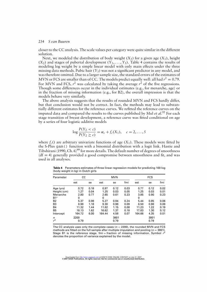
(X2) and stages of pubertal development (Y1, . . . ,Y3). Table 4 contains the results ofmodeling log weight by a simple linear model with only main effects under the threemissing data methods. Pubic hair (Y3)was not a significant predictor in any model, andwas therefore omitted. Due to a larger sample size, the standard errors of the estimates ofMVNor FCS are smaller than of CC. Themodels predict equally well: all had r2 = 0.79.For MVN and FCS, r2 was calculated by taking the average r2 of the five regressions.Though some differences occur in the individual estimates (e.g., for menarche, age) orin the fraction of missing information (e.g., for B2), the overall impression is that themodels behave very similarly.The above analysis suggests that the results of rounded MVN and FCS hardly differ,

but that conclusion would not be correct. In fact, the methods may lead to substan-tially different estimates for the reference curves. We refitted the reference curves on theimputed data and compared the results to the curves published by Mul et al.95 For eachstage transition of breast development, a reference curve was fitted conditional on ageby a series of four logistic additive models

logP(Y2 < c)

P(Y2 ≥ c)= αc + fc(X1), c = 2, . . . , 5

where fc() are arbitrary univariate functions of age (X1). These models were fitted bythe S-Plus gam() function with a binomial distribution with a logit link. Hastie andTibshirani (1990, Ch. 6)99 formore details. The default number of degrees of smoothness(df = 4) generally provided a good compromise between smoothness and fit, and wasused in all analyses.

Table 4 Parameters estimates of three linear regression models for predicting 100 log(body weight in kg) in Dutch girls

Parameter CC MVN FCS

est se est se fmi est se fmi

Age (yrs) 0.72 0.18 0.97 0.12 0.03 0.77 0.12 0.02Height (cm) 1.27 0.04 1.25 0.03 0.05 1.25 0.03 0.01Menarche 2.80 0.77 2.65 0.61 0.23 3.85 0.90 0.23B1∗ 0 0 0B2 5.37 0.98 5.27 0.94 0.24 5.44 0.85 0.06B3 8.98 1.18 9.30 0.98 0.09 8.50 0.98 0.08B4 11.32 1.44 11.82 1.15 0.08 11.23 1.22 0.19B5 18.13 1.62 16.62 1.37 0.18 17.83 1.30 0.12Intercept 164.72 6.00 164.44 4.58 0.07 164.66 4.35 0.01

n 2200 3801 3801r2 0.79 0.79 0.79

The CC analysis uses only the complete cases (n = 2200), the rounded MVN and FCSmethods are fitted on the full sample after multiple imputation and pooling (n = 3801).Stage B1 is the reference stage. fmi = fraction of missing information. Symbol r2

denotes the proportion of variance explained by the model.



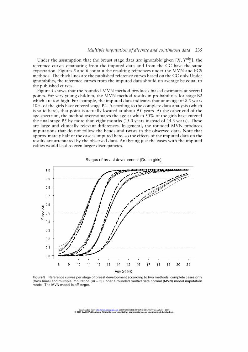
Under the assumption that the breast stage data are ignorable given [X,Yobs−2 ], thereference curves emanating from the imputed data and from the CC have the sameexpectation. Figures 5 and 6 contain the resulting references under the MVN and FCSmethods. The thick lines are the published reference curves based on the CC only. Underignorability, the reference curves from the imputed data should on average be equal tothe published curves.Figure 5 shows that the rounded MVN method produces biased estimates at several

points. For very young children, the MVN method results in probabilities for stage B2which are too high. For example, the imputed data indicates that at an age of 8.5 years10% of the girls have entered stage B2. According to the complete data analysis (whichis valid here), that point is actually located at about 9.0 years. At the other end of theage spectrum, the method overestimates the age at which 50% of the girls have enteredthe final stage B5 by more than eight months (15.0 years instead of 14.3 years). Theseare large and clinically relevant differences. In general, the rounded MVN producesimputations that do not follow the bends and twists in the observed data. Note thatapproximately half of the case is imputed here, so the effects of the imputed data on theresults are attenuated by the observed data. Analyzing just the cases with the imputedvalues would lead to even larger discrepancies.

Figure 5 Reference curves per stage of breast development according to two methods: complete cases only(thick lines) and multiple imputation (m = 5) under a rounded multivariate normal (MVN) model imputationmodel. The MVN model is off target.


236 S van Buuren

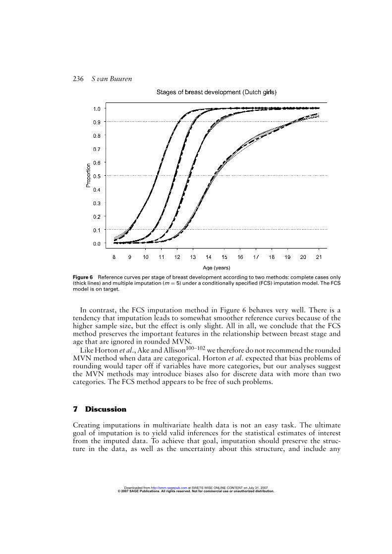
Figure 6 Reference curves per stage of breast development according to two methods: complete cases only(thick lines) and multiple imputation (m = 5) under a conditionally specified (FCS) imputation model. The FCSmodel is on target.

In contrast, the FCS imputation method in Figure 6 behaves very well. There is atendency that imputation leads to somewhat smoother reference curves because of thehigher sample size, but the effect is only slight. All in all, we conclude that the FCSmethod preserves the important features in the relationship between breast stage andage that are ignored in rounded MVN.LikeHorton et al., Ake andAllison100–102we therefore do not recommend the rounded

MVN method when data are categorical. Horton et al. expected that bias problems ofrounding would taper off if variables have more categories, but our analyses suggestthe MVN methods may introduce biases also for discrete data with more than twocategories. The FCS method appears to be free of such problems.

7 Discussion

Creating imputations in multivariate health data is not an easy task. The ultimategoal of imputation is to yield valid inferences for the statistical estimates of interestfrom the imputed data. To achieve that goal, imputation should preserve the struc-ture in the data, as well as the uncertainty about this structure, and include any



knowledge about the process that generated the missing data. Two main approacheshave been proposed, JM and FCS. JM stays close to the theory and leads to impu-tation procedures whose statistical properties are known under a correctly specifiedmodel. FCS is its semi-parametric and flexible cousin that emphasizes features in thedata.Several authors have been critical on JM in particular contexts. Schenker and Taylor54

performed a simulation study and observed that ‘the fully parametric method breaksdown in several situations, whereas the partially parametric methods maintain theirgood performance’. Belin et al.103 assessed the usefulness of the general location modelfor a mental health services study and conclude: ‘Our investigations suggest that eitherthe model or the companion assumption of ignorable nonresponse are not suitable inour applied context with numerous variables and a complicated pattern of missingdata.’ Gelman and Raghunathan104 address the difficulty of maintaining consistenciesin the imputed data and note that ‘separate regressions often make more sense thanjoint models’. Briggs et al.105 imputed cost data and wrote ‘using the algorithm basedon multivariate normality resulted in failure of the algorithm to converge’, and wereforced to dichotomize their data. In order to bypass the limitations of joint models,Gelman (p. 541) concludes: ‘Thus we are suggesting the use of a new class of models –inconsistent conditional distributions – that were initially motivated by computationaland analytical convenience.’83

Within the JM context, the data often need to be transformed before imputation(to make the observed data conform to the imputation model) and after impu-tation (to make the imputed values conform to the observed data) (Schafer, 1997p. 147–148, 202–203, 214, 272, 374).7 While such transformations enhance the per-formance of the JM. Various authors100–102 observed that rounding imputed values tothe closest observed value in the data can introduce a bias in the parameter estimates,whereas if the imputed data are not rounded, no bias would occur. Our analysis ofthe pubertal data provide evidence that rounding bias in JM may also show up in reallife categorical data with more than two categories. Chen et al.107 also provide somesupport for the idea that normal methods do not work well for ordinal data. Our anal-ysis of the pubertal data showed that FCS appears to be less sensitive to such biases.We therefore recommend that continuous data are imputed as continuous and discretedata are imputed as discrete. Conditional specification is the most convenient way to dothat. Despite its theoretical weaknesses, we conclude that FCS is a useful and flexiblealternative to JM when the joint distribution of the data is not easily specified.Missing data problems require careful consideration and thought. It will be clear by

now thatMI is not an automatic technical fix for the missing data. Rather, it is a generaland principled strategy for attacking missing data problems. The process of specifyingthe imputationmodel is a scientificmodeling activity on its own, that comeswith its ownmodel building principles. The fact that highly automated and sophisticated proceduresare available does not free the imputer or the analyst from the responsibility to considerthe appropriateness of the assumptions underlying the imputationmodel for the problemat hand. The implication is that medical researchers should include a short descriptionof their missing data method into their scientific articles. The most natural location forthat description is the section on the statistical analysis.


238 S van Buuren

Acknowledgement

I thank Peter van der Heijden, Ian White and Patrick Royston for their constructive andinsightful feedback on an earlier draft of this paper.

References

1 Rubin DB.Multiple imputation fornonresponse in surveys. Wiley, 1987.

2 Rubin DB. Multiple imputation after 18+years. Journal of the American StatisticalAssociation 1996; 91(434): 473–89.

3 Collins LM, Schafer JL, Kam CM. Acomparison of inclusive and restrictivestrategies in modern missing dataprocedures. Psychological Methods 2001;6(3): 330–51.

4 Scheuren F. Multiple imputation: how itbegan and continues. AmericanStatistician 2005; 59(4): 315–9.

5 Dempster AP, Laird NM, Rubin DB.Maximum likelihood estimation fromincomplete data via the EM algorithm(with discussion). Journal of the RoyalStatistical Society Series B: StatisticalMethodology 1977; 39: 1–38.

6 Little RJA, Rubin DB. Statistical analysiswith missing data. second edition Wiley,2002.

7 Schafer JL. Analysis of incompletemultivariate data. Chapman & Hall,1997.

8 Schafer JL. Multiple imputation: a primer.Statistical Methods in Medical Research1999; 8(1): 3–15.

9 Stern HS, Sinharay S, Russell D. The use ofmultiple imputation for the analysis ofmissing data. Psychological Methods 2001;6(3): 317–29.

10 Allison PD.Missing data. Sage, 2002.11 Schafer JL, Graham JW. Missing data: our

view of the state of the art. PsychologicalMethods 2002; 7(2): 147–77.

12 Rubin DB, Schenker N. Multipleimputation in health-care databases: anoverview and some applications. Statisticsin Medicine 1991; 10(4): 585–98.

13 Barnard J, Meng XL. Applications ofmultiple imputation in medical studies:from AIDS to NHANES. StatisticalMethods in Medical Research 1999; 8(1):17–36.

14 Greenland S, Finkle WD. A critical look atmethods for handling missing covariatesin epidemiologic regression analyses.American Journal of Epidemiology 1995;142(12): 1255–64.

15 Kmetic A, Joseph L, Berger C, TenenhouseA. Multiple imputation to account formissing data in a survey: estimating theprevalence of osteoporosis. Epidemiology2002; 13(4): 437–44.

16 AbrahamWT, Russell DW. Missing data: areview of current methods and applicationsin epidemiological research. CurrentOpinion in Psychiatry 2004; 17(4): 315–21.

17 Croy CD, Novins DK. Methods foraddressing missing data in psychiatric anddevelopmental research. Journal of theAmerican Academy of Child andAdolescent Psychiatry 2005; 44(12):1230–40.

18 Kneipp SM, McIntosh M. Handlingmissing data in nursing research withmultiple imputation.Nursing Research2001; 50(6): 384–9.

19 Patrician PA. Multiple imputation formissing data. Research in Nursing andHealth 2002; 25(1): 76–84.

20 McCleary L. Using multiple imputationfor analysis of incomplete data in clinicalresearch.Nursing Research 2002; 51(5):339–43.

21 Fox-Wasylyshyn SM, El-Masri MM.Handling missing data in self-reportmeasures. Research in Nursing and Health2005; 28(6): 488–95.

22 Molenberghs G, Burzykowski T, MichielsB, Kenward MG. Analysis of incompletepublic health data. Revue d’Epidemiologieet de Sante Publique 1999; 47(6): 499–514.

23 Zhou XH, Eckert GJ, Tierney WM.Multiple imputation of public healthresearch. Statistics in Medicine 2001;20(9–10): 1541–9.

24 Raghunathan TE. What do we do withmissing data? Some options for analysis of



incomplete data. Annual Review of PublicHealth 2004; 25: 99–117.

25 Crawford SL, Tennstedt SL, McKinlay JB.A comparison of analytic methods fornon-random missingness of outcome data.Journal of Clinical Epidemiology 1995;48(2): 209–19.

26 Faris PD, Ghali WA, Brant R, Norris CM,Galbraith PD, Knudtson ML, APPROACHInvestigators. Multiple imputation versusdata enhancement for dealing with missingdata in observational health care outcomeanalyses. Journal of Clinical Epidemiology2002; 55(2): 184–91.

27 Oostenbrink JB, Al MJ. The analysis ofincomplete cost data due to dropout.Health Economics 2005; 14(8): 763–76.

28 Chavance M. Handling missing items inquality of life studies. Communications inStatistics – Theory and Methods 2004;33(6): 1371–83.

29 Catellier DJ, Hannan PJ, Murray DM,Addy CL, Conway TL, Yang S, Rice JC.Imputation of missing data whenmeasuring physical activity byaccelerometry. Med Sci Sports Exerc 2005;37(11 Suppl): S555–62.

30 Wood AM, White IR, Hillsdon M,Carpenter J. Comparison of imputationand modelling methods in the analysis of aphysical activity trial with missingoutcomes. International Journal ofEpidemiology 2005; 34(1): 89–99.

31 Smits N, Mellenbergh GJ, Vorst HCM.Alternative missing data techniques tograde point average: Imputing unavailablegrades. Journal of EducationalMeasurement 2002; 39(3): 187–206.

32 Peugh JL, Enders CK. Missing data ineducational research: a review of reportingpractices and suggestions forimprovement. Review of EducationalResearch 2004; 74(4): 525–56.

33 Walczak B, Massart DL. Dealing withmissing data: part II. Chemometrics andIntelligent Laboratory Systems 2001; 58(1):29–42.

34 Longford NT. Multilevel analysis withmessy data. Statistical Methods in MedicalResearch 2001; 10(6): 429–44.

35 Olinsky A, Chen S, Harlow L. Thecomparative efficacy of imputationmethods for missing data in structuralequation modeling. European Journal ofOperational Research 2003; 151(1): 53–79.

36 Allison PD. Missing data techniques forstructural equation modeling. Journal ofAbnormal Psychology 2003; 112(4):545–57.

37 Twisk J, de Vente W. Attrition inlongitudinal studies: how to dealwith missing data. Journal ofClinical Epidemiology 2002; 55(4):329–37.

38 Demirtas H. Modeling incompletelongitudinal data. Journal of ModernApplied Statistical Methods 2004; 3(2):305–21.

39 Streiner DL. The case of the missing data:Methods of dealing with dropouts andother research vagaries. Canadian Journalof Psychiatry 2002; 47(1): 68–75.

40 Kristman VL, Manno M. Methods toaccount for attrition in longitudinal data:do they work? A simulation study.European Journal of Epidemiology 2005;20(8): 657–62.

41 Little R, Yau L. Intent-to-treat analysisfor longitudinal studies withdrop-outs. Biometrics 1996; 52(4):1324–33.

42 Liu G, Gould AL. Comparison ofalternative strategies for analysis oflongitudinal trials with dropouts. Journalof Biopharmaceutical Statistics 2002;12(2): 207–26.

43 Houck PR, Maz umdar S, Koru-Sengul T,Tang G, Mulsant BH, Pollock BG,Reynolds CF 3rd. Estimating treatmenteffects from longitudinal clinical trial datawith missing values: Comparative analysesusing different methods. PsychiatryResearch 2004; 129(2): 209–15.

44 Tang L, Unntzer J, Song J, Belin TR. Acomparison of imputation methods in alongitudinal randomized clinical trial.Statistics in Medicine 2005; 24(14):2111–28.

45 Beunckens C, Molenberghs G, KenwardMG. Direct likelihood analysis versussimple forms of imputation for missingdata in randomized clinical trials. ClinicalTrials 2005; 2(5): 379–86.

46 Barnes SA, Lindborg SR, Seaman J.Multiple imputation techniques in smallsample clinical trials. Statistics in Medicine2006; 25(2): 233–45.

47 Pigott TD. Missing predictors in models ofeffect size. Evaluation and the HealthProfessions 2001; 24(3): 277–307.


240 S van Buuren

48 Ibrahim JG, Herring AH, Chen MH,Lipsitz SR. Missing-data methods forgeneralized linear models: a comparativereview. Journal of the American StatisticalAssociation 2005; 100(469): 332-46.

49 Schafer JL. Multiple imputation inmultivariate problems when theimputation and analysis models differ.Statistica Neerlandica 2003; 57(1): 19–35.

50 Brand JPL, Van Buuren S,Groothuis-Oudshoorn K, Gelsema ES.A toolkit in SAS for the evaluation ofmultiple imputation methods. StatisticaNeerlandica 2003; 57(1): 36–45.

51 Meng XL. Multiple imputation withuncongenial sources of input (withdiscussion). Statistical Science 1995; 10:538–73.

52 Van Buuren S, Boshuizen HC, Knook DL.Multiple imputation of missing bloodpressure covariates in survival analysis.Statistics in Medicine 1999; 18(6): 681–94.

53 Abayomi K, Gelman A, Levy M.Diagnostics for multivariate imputations.Assessed from Gelman’s weblog November2005.

54 Schenker N, Taylor JMG. Partiallyparametric techniques for multipleimputation. Computational Statistics andData Analysis 1996; 22(4): 425–46.

55 Rubin DB. Statistical matching usingfile concatenation with adjusted weightsand multiple imputations. Journal ofBusiness Economics and Statistics 1986; 4:87–94.

56 Little RJA. Missing data adjustments inlarge surveys (with discussion). Journal ofBusiness Economics and Statistics 1988; 6:287–301.

57 Harrell F. Regression modeling strategies,with applications to linear models, logisticregression, and survival analysis Springer,2001.

58 Albert JH, Chib S. Bayesian analysis ofbinary and polychotomous variables.Journal of the American StatisticalAssociation 1993; 88: 669–79.

59 Yucel RM, Zaslavsky AM. Imputation ofbinary treatment variables withmeasurement error in administrative data.Journal of the American StatisticalAssociation 2005; 100(472): 1123–32.

60 Brand JPL. Development, implementationand evaluation of multiple imputationstrategies for the statistical analysis of

incomplete data sets. Erasmus University,1999.

61 Raghunathan TE, Lepkowski JM, vanHoewyk J, Solenberger P. A multivariatetechnique for multiply imputing missingvalues using a sequence of regressionmodels. Survey Methodology 2001; 27:85–95.

62 Parzen M, Lipsitz SR, Fitzmaurice GM.A note on reducing the bias of theapproximate Bayesian bootstrapimputation variance estimator. Biometrika2005; 92(4): 971–4.

63 Reilly M, Pepe M. The relationshipbetween hot-deck multiple imputation andweighted likelihood. Statistics in Medicine1997; 16(1–3): 5–19.

64 Junninen H, Niska H, Ruuskanen J,Kolehmainen M, Tuppurainen K. Methodsfor imputation of missing values in airquality data sets. AtmosphericEnvironment 2004; 38(18): 2895–907.

65 Paddock SM. Bayesian nonparametricmultiple imputation of partially observeddata with ignorable nonresponse.Biometrika 2002; 89(3): 529–38.

66 Heckman JJ. The common structure ofstatistical models of truncation, sampleselection and limited dependent variablesand a simple estimator for such models.Annals of Economic and SocialMeasurement 1976; 5: 475–92.

67 Greenlees WS, Reece JS, Zieschang KD.Imputation of missing values whenthe probability of response depends on thevariable being imputed. Journal ofthe American Statistical Association 1983;77: 251–61.

68 Wei GCG, Tanner MA. Applications ofmultiple imputation to the analysis ofcensored regression data. Biometrics 1991;47(4): 1297–309.

69 Pan W, Connett JE. A multiple imputationapproach to linear regression withclustered censored data. Lifetime DataAnalysis 2001; 7(2): 111–23.

70 Goetghebeur E, Ryan L. Semiparametricregression analysis of interval-censoreddata. Biometrics 2000; 56(4): 1139–44.

71 Pan W. A multiple imputation approach toCox regression with interval-censoreddata. Biometrics 2000; 56(1): 199–203.

72 Bechger TM, Boomsma DI, Koning H.A limited dependent variable model forheritability estimation with non-random



ascertained samples. Behavior Genetics2002; 32(2): 145–51.

73 Hopke PK, Liu C, Rubin DB. Multipleimputation for multivariate data withmissing and below-thresholdmeasurements: time-series concentrationsof pollutants in the arctic. Biometrics 2001;57(1): 22–33.

74 Lubin JH, Colt JS, Hartge P, Camann D,Davis S, Cerhan JR, Severson RK,Bernstein L, Hartge P. Epidemiologicevaluation of measurement data in thepresence of detection limits.Environmental Health Perspectives 2004;112(17): 1691–6.

75 Fridley B, Rabe K, de Andrade M.Imputation methods for missing data forpolygenic models. BMC Genetics 2003;4(Suppl 1): S42.

76 Heeringa SG, Little RJA, RaghunathanTE. Multivariate imputation of coarsenedsurvey data on household wealth. InGroves RM, Dillman DA, Eltinge JL, LittleRJA, eds. Survey Nonresponse. Wiley,2002.

77 Rubin DB, Schafer JL. Efficiently creatingmultiple imputations for incompletemultivariate normal data. 1990Proceedings of the Statistical ComputingSection, American Statistical Association1990; 83–8.

78 Rubin DB. Nested multiple imputation ofNMES via partially incompatible MCMC.Statistica Neerlandica 2003; 57(1): 3–18.

79 Van Buuren S, Brand JPL,Groothuis-Oudshoorn K, Rubin DB. Fullyconditional specification in multivariateimputation. Journal of StatisticalComputation and Simulation 2006; 76(12):1049–1064.

80 Horton NJ, Lipsitz SR. Multipleimputation in practice: comparison ofsoftware packages for regression modelswith missing variables. AmericanStatistician 2001; 55: 244–54.

81 Kennickell AB. Imputation of the1989 survey of consumer finances:stochastic relaxation and multipleimputation. ASA 1991 Proceedings of theSection on Survey Research Methods 1991;1–10.

82 Heckerman D, Chickering DM, Meek C,Rounthwaite R, Kadie C. Dependencynetworks for inference, collaborativefiltering, and data visualisation. Journal of

Machine Learning Research 2001; 1:49–75.

83 Gelman A. Parameterization and BayesianModeling. Journal of the AmericanStatistical Association 2004; 99(466):537–45.

84 Van Buuren S, Groothuis-Oudshoorn K.Multivariate imputation by chainedequations: MICE V1.0 user’s manual.TNO Quality of Life, 2000,PG/VGZ/00.038.

85 Arnold BC, Castillo E, Sarabia JM.Conditional specification of statisticalmodels. Springer, 1999.

86 Goodman LA. The multivariate analysis ofqualitative data: interactions amongmultiple classifications. Journal of theAmerican Statistical Association 1970; 65:226–56.

87 Besag J. Spatial interaction and thestatistical analysis of lattice systems.Journal of the Royal Statistical SocietySeries B: Statistical Methodology 1974; 36:192–236.

88 Arnold BC, Press SJ. Compatibleconditional distributions. Journal of theAmerican Statistical Association 1989; 84:152–6.

89 Gelman A, Speed TP. Characterizing ajoint probability distribution byconditionals. Journal of the RoyalStatistical Society Series B: StatisticalMethodology 1993; 55: 185–8.

90 Gelman A, Rubin DB. Inference fromiterative simulation using multiplesequences (with discussion). StatisticalScience 1991; 7: 457–511.

91 Royston P. Multiple imputation of missingvalues. The Stata Journal 2004; 4: 227–41.

92 Royston P. Multiple imputation of missingvalues: update of ice. Stata Journal 2005; 5:527–36.

93 Fredriks MA, van Buuren S, Burgmeijer RJ,Meulmeester JF, Beuker RJ,Brugman E, Roede MJ,Verloove-Vanhorick SP, Wit JM.Continuing positive secular growth changein The Netherlands 1955–1997. PediatricResearch 2000; 47: 316–23.

94 Marshall WA, Tanner JM. Variations inpattern of pubertal changes in girls.Archives of Diseases in Childhood 1969;44: 291–303.

95 Mul D, Van Buuren S, Frediks MA,Oostdijk W, Verloove-Vanhorick SP,


242 S van Buuren

Wit JM. Pubertal development in TheNetherlands 1965–1997. Pediatric Research2001; 50: 479–86.

96 Little RJA. Regression with missing X’s: areview. Journal of the American StatisticalAssociation 1992; 87: 1227–37.

97 McCullagh P, Nelder JA eds. Generalizedlinear models, second edition. Chapman &Hall, 1989.

98 Venables WN, Ripley BD eds. Modernapplied statistics with S, fourth editionSpringer-Verlag, 2002.

99 Hastie TJ, Tibshirani RJ. Generalizedadditive models. Chapman & Hall, 1990.

100 Horton NJ, Lipsitz SR, Parzen M. Apotential for bias when rounding inmultiple imputation. American Statistician2003; 57(4): 229–32.

101 Ake CF. Rounding after multipleimputation with non-binary categoricalcovariates SUGI 30 Proceedings 2005,112–30, pp. 1–11.

102 Allison PD. Imputation of categoricalvariables with PROCMI . SUGI 30Proceedings 2005, 113–30,pp. 1–14.

103 Belin TR, Hu MY, Young AS, Grusky O.Performance of a general location modelwith an ignorable missing-dataassumption in a multivariate mental healthservices study. Statistics in Medicine 1999;18: 3123–35.

104 Gelman A, Raghunathan TE. Discussionof Arnold et al. Conditionally specifieddistributions. Statistical Science 2001; 16:249–74.

105 Briggs A, Clark T, Wolstenholme J, ClarkeP. Missing . . . . presumed at random:cost-analysis of incomplete data.HealthEconomics 2003; 12: 377–92.

106 Chen L, Valois RF, Toma-Drane M, DraneJW. Multiple imputation for missingordinal data. Journal of Modern AppliedStatistical Methods 2005; 4(1): 288–99.


Documents

Multiple imputation of discrete and continuous data by ... by FCS - SMMR 2007.pdf · Multiple imputation of discrete and continuous data by fully conditional speciﬁcation ... 2.2