Embed Size (px)
Citation preview

IB 64/5 Oslo, 1. desember 1 964
Ref.; SN/AB 19/10-64
Multiple Regression and Correlation Analysis
Av Svein Nordbotten og Thor Aastorp
INNHOLD
1. General Description
2. Card Preparation ..
s.
s.
1
2
3. Order of Cards s 5
4. Logical Units ..... s. 6
5. References ........ s. 6
Appendix 1 0.000000000 S. 7
Appendix 2 ........... s. 12
Statistisk sentralbyrå
II Ill I 1 ,11 1 ,1,11 111 II II
Dette notat er et internt arbeidsdokument og må ikke offentliggjøres eller sendes andre etater, institusjonere. l., verken i sin helhet eller i utdrag.

SN/AB, 19/10-64
1)MULTIPLE REGRESSION AND CORRELATION ANALYSIS
1. GENERAL DESCRIPTION
a. This program is a modification and extension of BIND 29. The primary
modification is that the independent variables are listed in the order of
their importance based on the reduction of sum of squares of the dependent
variable attributable successively to each independent variable.
Additional output includes cumulative: (1) standard errors of estimate,
(2) sums of squares (3) proportions of variance, (4) F-values, and
(5) multiple correlation coefficients.
b. The maximum number of variables which can be processed by this program
is 50 variables.
C. The upper limitation on sample size is 99,999 9 and the lower limitation
on sample size is two greater than the number of variables.
d. This program can perform a different transformation of any variable and
generate new variables if desired, according to the codes specified in
Trans-generation cards. A transgeneration can be made conditional if
desired, according to the condition codes specified in the Trans-generation
cards. Any number of variables can be generated, but the total number
of variables must not exceed 50.
e. Any variable, original or generated can be named the dependent variable.
There is no limit to the number of replacements.
f. The maximum number of variables which can be deleted at one time is 32.
However, there is no limit to the number of deletions of different sets of
variables.
g. The format for input data must be specified in the Variable Format Card(s).
h. The sums sums of squares and cross-products, in the format produced by
this program, can in a later run be used as input if additional replacements
and deletions are required.
1) This program and its description are both modifications of the BIMD 29
program and is copied only for use within the Central Bureau of Statistics.

Col. 3-6
Col. 7,8 Number of original variables,
Col. 9-1 7 Sample size, n
Problem number (May be alphabetical characters
Col. 71,72
Col. 80
k variable format•cards 5)
1 1 sums, sums of squares and cross-products
2
2. CARD PREPARATION
a. CONTROL CARDS
b. PROGRAM CONTROL CARDS
(1) PROBLEM CARD (One Problem Card for each problem)
Col. 1,2 PR (for PRoblem Card)
Col. 14-16 000 no trans-genration
m m trans-generation cards (m 99)
Col. 17,18 00 no variables added to original set after
trans-generation
q q variables added to original set after
trans-generation
Co?. 19-21 Number of Replacement and Deletion. Cards
Col. 22-26 Per cent of sum of squares to limit variables
entering in a regression model. Keypunch a
value with a decimal point. (See Note 1 below
is used as input
Note: (1) The choice of percentage value for limiting
variable will depend upon the purpose of the
analysis. A suggested trial value is one per
cent, 0.01. If all independent variables are
to be included in a regression model, keypunch
0.0.
(2) TRANS-GENERATION CARD(S)
If a non-zero number is specified in Col. 14- .16 of the
Problem Card the same number of Trans-generation
Card(s) must be prepared. Different types of transformation
can be performed successively on the same variable, if
desired. The format of Trans-generation Card is as follows:

Col. 1,2 TR (for TRans -generation Card)
Col. 3,4 Variable number to be assigned on transformed
or generated variables
Col. 5,6 Transformation code. Codes 01 9 02, ... 14 of
the transgeneration list may be used. (See
Appendix 2)
Col. 7 9 8 A-variable number
Co?. 9-14 B-variable number or constant C (keypunch with
decimal point). If the constant is a negative value,
keypunch a minus sign to the left of the constant.
Col. 15-16 Condition code. Codes 01 02 ••., 12 of the condition
list may be used. (See Appendix 2)
Co?. 17-18 M-variable number
Col. 19-24 N-variable number or constant K (keypunch with
decimal point). If the constant is a negative value,
keypunch a minus to the left of the constant
VARIABLE NAME CARD(S)
The purpose of Variable Name Card(s) is to identify the
variables in the output by their names. The format of
Variable Name Card is as follows:
Col. 1-8 Name of 1st variable
Col. 9-16 Name of 2nd variable
Co?. 17-24 Name of 3rd variable
Co?. 73-80 Name of 10th variable
If there are more than 10 variables, continue keypunching
on the second card in the same manner.
If variables are to be generated, the names of these variables
must also be keypunched in addition to those of the original
variables.
If the identification of the variables by their names is not
desired, use blank card(s) for this purpose. Variable Name
Card(s) must be present.

STANDARD SCALE CARD(S)
The purpose of the Standard Scale Cards is to scale the original
variables by 10e. The exponents are specified in the Standard Scale
Card(s) as follows:
Col. 1-8 Scale factor for the 1st original variable
Col. 73-80 Scale factor for thelOth original variable
If there are more than ten- variables, scale factor specification
is continued on a second Card in the same manner. Decimal point
may be punched. The standard scale cards must be present.
VARIABLE FORMAT CARD(S)
The same number of Variable Format Card(s) as specified in col. 71 and
72 of the Problem Card must be prepared. The variable format
description can use all 80 columns.
(6) REPLACEMENT AND DELETION CARD (S
This card, RD Card, has a fourfold purpose:
1) It indicates the replacement of the dependent variable
2) It indicates the deletion of variables
3) It indicates a replacement and deletion, and
4) It controls the output.
The replacement of a dependent variable and deletion of
different sets of variables can be made as many times as
desired. This means that it is possible to make multiple
re -Pression and correlation analyses with selected sets of
variables. The program will retain all the variables, original
and generated, until all R - D Cards for one problem are
processed.
The program does not give any multiple regression and correlation
analysis unless R D Cards are prepared. R D Card(s) must be
present, and the number of R D Card(s) prepared must agree with
the number specified in Col. 19-21 of the Problem Card.
The format of R - D Card is as follows:
Co?. 1,2 RD (for Replacement and Deletion Card)
Col. 3,4 02 If the table of residuals and analysis of extreme
(4)
(5)

residuals are desired. (See Note 2 below).
01 if only the analysis of extreme residuals
is desired.
00 if neither one is desired.
Col. 5,6 A variable to be treated as the dependent
variable.
Col. 7,8 Total number of variables to be deleted.
Col. 9,10 1st variable to be deleted.
Co?. 11 12 2nd variable to be deleted
Co?. 71,72 32nd variable to be deleted
Note: (2) Then the sample size is large, 02 punch should not
be used.
The maximum number of variables which can be deleted
at one time is 32.
Although replacements and deletions are repeated over and
over again, the arramgement of variables will not change.
Therefore, the number of the next dependent variable and
the numbers of variables to be deleted must be stated in
terms of the basic set of variables, which may be the
original set of variables or the set of variables after
trans-generation.
Delete low numbered variables first; namely, X2 comes
first and then X7 .
(7) FINISH CARD
This card will notify the program of the end of the entire job.
This card has the following format:
Co?. 1-6 FINISH
c. STANDARD INPUT DATA RECORDS
This records can be read either from cards or magnetic tape.
3. ORDER OF CARDS
More than one problem can be processed consecutively. The following
example illustrates the order of cards:

0 0 •
1) Problem Card for the first problem Log.unit. 4
2) Trans-generation Cards (if used) tt 4
3) Variable Name Cards It 4
4) Scale Card(s) II 4
5) Variable Format Cards it 4
6) Input Data Cards or Tape li 3
7) R-D Card(s) ?I 4
0 • •
•. Problem Card for the last problem Log.unit. 4
. . Trans-generation Cards (if used) ti 4
. • Variable Name Cards it 4
.. Scale Card(s) II 4
.. Variable Format Cards 4
.. Input Data Cards or Tape 3t,
.. R-D Card(s) 11 4
. • Finish. Card If 4
4. LOGICAL UNITS
a) Logical Unit 2 is used for output
b) Logical Unit 3 is used for input data
c) Logical Unit 4 is used for Program Control Cards
d) Logical Unit 5 is used as intermidiate store
REFERENCES
a. Dixon and Massey, Introduction to pp 275-278.
McGraw-Hill Book Company, Inc.; 1957.
b. Ostle, Bernard, Statistics in research; Chapter 8.
The Iowa 0 -bate College Press; 1954.
C. Bennett and Franklin, Statistical Ari,LLLILI_LE_LLEIELLTLILLILL .
Chemical Industry; Appendix 6k. John Wiley and Sons, Inc.; 1954.

7
APPENDIX I
Computational Procedures
Model assumed:
Y is normally distributed with mean p and variance cr2
where k = A p1x1 + 43 2x2 + + X.
The computation steps performed by the program follow:
Step I. Preliminary computations.
(1) Trans-generation: If desired, data are transformed and/or
generated according to the codes specified in the Trans-generation
Cards.
Sums: x. i = 1,2 p
where p is the number of variables.
2Sums of squares: E X.
X.Means: = n where n is sample size.
Standard deviations:
Cross product sums:
P. i = 1,2 1 ... l p
= 1,2 9 .00,p
Cross product of deviations:
D.. =1:(X. R.)(x.j
Simple correlation coefficients:
r. R.)(x.;.)
Step 2. The program reads the Replacement and Deletion Card and performs
the following computations:
(1) Rearrange the variables in the cross product of deviation
matrix and construct a.. in the working storage area.ij
(7)
(8)
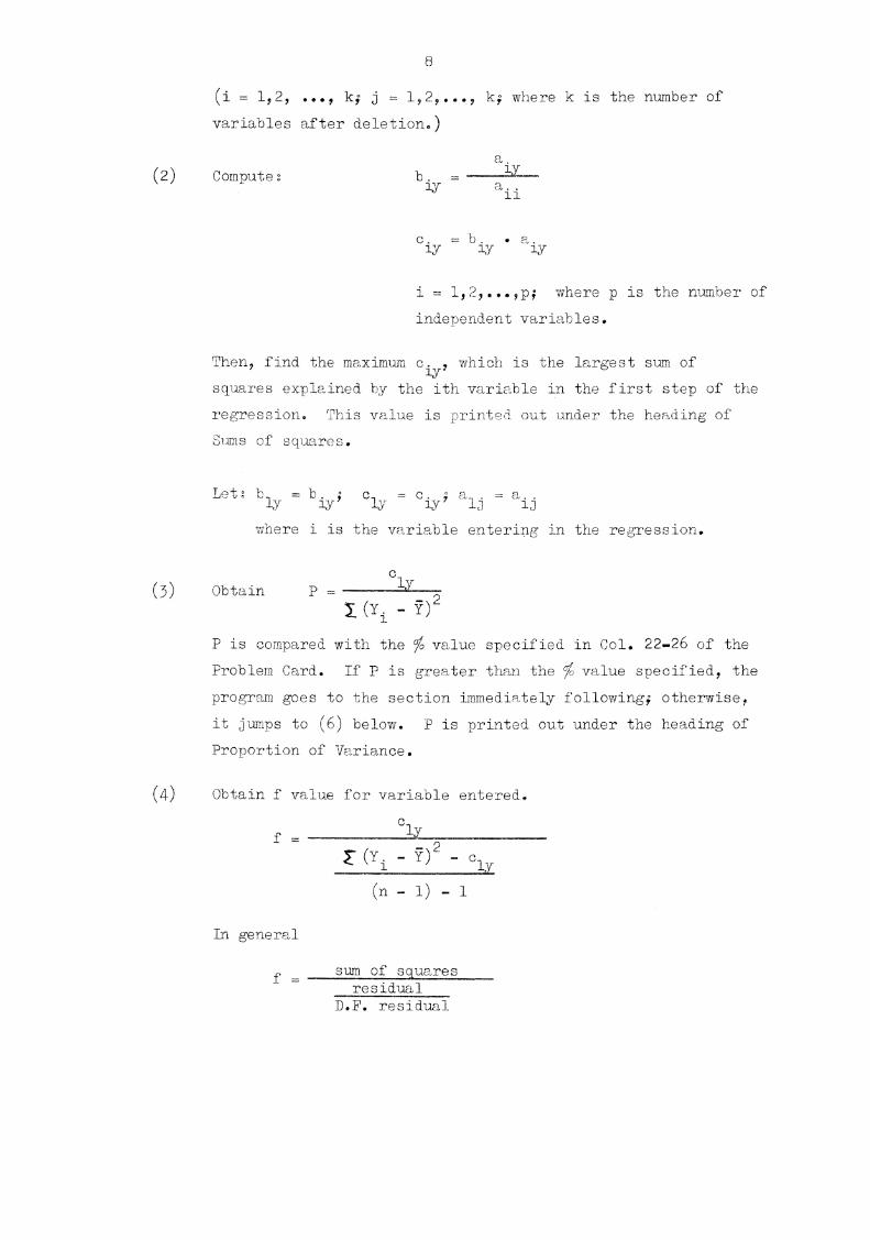
(i = 1,2, k; j = 1,2 k- where k is the number of
variables after deletion.
(2) Compute: b. .ly a..
C. .ly ly ly
i = 1 1 2,...,p; where p is the number of
independent variables.
Then, find the maximum c. which is the largest sum ofly
squares explained by the ith variable in the first step of the
regression. This value i printed out under the heading of
Sums of squares.
Let: b y. Y; cly o ily ; a,.
where i is the variable entering in the regression.
(3) Obtain P =- 7 ) 2
P is compared with the % value specified in Co?. 22-26 of the
Problem Card. If P is greater than the % value specified the
program goes to the section immediately following; otherwise,
it jumps to (6) below. P is printed out under the heading of
Proportion of Variance.
(4 )
Obtain f value for variable entered.
f = ly
(Y. - 7) 2 cly
- 1) -
In general
f =residual
B.F. residual

(5) Compute:
a.blj a
ll
a. = a..-a. b .10 10
where p is the number of
independent variables
i 2,3,..., k
k
where k is the number of variables
including the dependent variable.
The sections (2) - (5) above are repeated to select and enter the
remaining variables in the regression in the order of their
contribution to the sum of squares of the dependent variable.
(6) Compute cumulative regression:
(a) Sums of squares:
kZ =..E. ck j jy k - 1 7 2,- , q
where q is the number of the
variables entered in the regression.
(b) Proportions of variances:
R2
=k
(c) Multiple correlation coefficients;
/ kRk = R
2
(d) Standard error of estimates:
-"Y -k
(e) F values:Zk Zk
Fk
k
n - k - 1
k
1 0
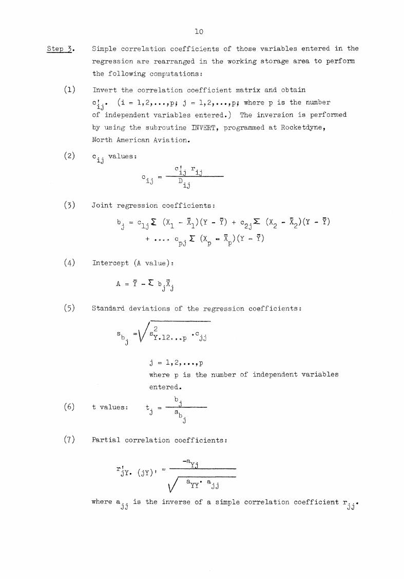
Step 3. Simple correlation coefficients of those variables entered in the
regression are rearranged in the working storage area to perform
the following computations:
(1) Invert the correlation coefficient matrix and obtain
clj . (i = 1,2 i 1,2,...,p; where p is the number
of independent variables entered.) The inversion is performed
by using the subroutine INVERT, programmed at Rocketdyne,
North American Aviation.
(2) C, . values
cl. r..ij0.. =
D..
(3) Joint regression coefficients:
b. . clj (x1 R1 )(Y. - 7) c2j (x - X2 )(Y
7
+ c (x .5"C )(Y 7)
Pi P P
(4) Intercept (k value)
(5) Standard deviations of the regression coefficients:
2s b. .c..
sY.12„—p JJ
j = 1 ,2,40 0 , , P
where p is the number of independent variables
entered.
b.(6) t values:
sb.
(7) Partial correlation coefficients:
-ayjr!JY. 0-0 1
ayy. ajj
where a.. is the inverse of a simple correlation coefficient3,1 JJ

11
(8) Compare check on final coefficient:
The last b. computed in the section (2) of Step 2 is also
the regression coefficient of the last independent variable. This
coefficient is printed out in order to check the accuracy of the
computing procedure explained above.
Step 4. Analysis of extreme residuals
The statistical procedure for detection of outliers explained by
Dixon and Massey is used in the program. This procedure
assumes that data are normally distributed and that they come
from the same population. Residuals are not classified in this
group. Therefore, readers are reminded that this statistical
procedure is only approximate.
Step 5. The program computes the Durbin - Watson d-statistic for testing
the presence of autocorrelated disturbances

12
APPENDIX 2
Transgeneration codes
00 : No transformation
01 xt = V
02 x' \/ x +
03 : x' - ln x
= ex04 x
05 xl sin-1
06 xt - sin-1 I x sin x. -1
n+107 : x' = 1 / x
08 x_ + c
09: x' = x • cc10 x1= x
11 : x XA
-i- XB12 : x' x
A xB
13 : x' - XA * XB
14 : xt =/xA x3
Condition codes
01 transgeneration if x - x T
02 : tIN
03 ) x,xTvi N
04 : x„, -., xDa N
05 , x < xl,,TTI fr-vi
06 x.1 .1- x1
.1
07 : - KxI\iT
08 : u ), K: 11,1
09 : u ,x \ K,ivl10 : l u x1 K1,411 n x( K
M12 : ff
X, . VJ....,ivr