Multiple Representations of Biological Processes · 2006-07-16 · Multiple Representations of Biological Processes 3 There are many variants of the Petri net formalism and a variety

Multiple Representations of Biological Processes

Carolyn Talcott1 and David L. Dill2

1 SRI [email protected] Stanford University

[email protected]

Abstract. This paper describes representations of biological processes based onRewriting Logic and Petri net formalisms and mappings between these represen-tations used in the Pathway Logic Assistant. The mappings are shown to preserveproperties of interest. In addition a relevant subnet transformation is defined, thatspecializes a Petri net model to a specific query to reduce the number of transi-tions that must be considered when answering the query. The transformation isshown to preserve the query in the sense that no answers are lost.

Keywords: signal transduction, biological process, Pathway Logic, Rewriting Logic,Petri Net

1 Introduction

Pathway Logic [1–3] is an approach to modeling cellular processes based on formalmethods. In particular, formal executable models of processes such as signal transduc-tion, metabolic pathways, and immune system cell-cell signaling are developed usingthe rewriting logic language Maude [4, 5] and a variety of formal tools are used to querythese models. An important objective of Pathway logic is to reflect the ways that biolo-gists think about problems using informal models, and to provide bench biologists withtools for computing with and analyzing these models that are natural.

Using the reflective capabilities of Maude, several alternative representations are de-rived to support use of different tools for visualization and analysis. The Pathway LogicAssistant (PLA) manages these different representations and, using the IOP+IMaudeframework [6], provides a user interface that supports visualization and interaction withthe models, and access to tools such as the Pathalyzer for carrying out in silico experi-ments. In particular, PLA uses Petri nets which provide visual representations and algo-rithms for answering reachability queries interactively, displaying the results in a waythat is natural for biologists.

Being able to use alternative representations with different expressive capabilitiesand tools for visualization and analysis is important both for managing complexity andbeing able to focus on different properties. In the presence of multiple representationsit is crucial to be able move between representations in semantically meaningful ways,preserving relevant properties. In this paper we describe a class of rewriting logic mod-els of biological processes and a mapping of these models to Petri net models. We showthat this mapping preserves computations and satisfaction of temporal formulae. Fi-nally, we describe transformations that specialize Petri net models to specific queries

2 Talcott and Dill

by reducing the set of transitions that need to be considered, and show that transforma-tions are safe in the sense that query results are not changed. Specializing simplifies aPetri net model and allows the user to focus attention on the part of the model relevantto the question under consideration.

Plan. The remainder of this paper is organized as follows. Related work is discussed in§2. To provide context and motivate the technical results, a brief overview of PathwayLogic and the ways that biologists can compute with and query Pathway Logic modelsis given in section 3. In section 4 the notion of occurrence-based rewrite theory is de-fined and mappings between such theories and Petri net models are defined and showncorrect. The notion of subnet relevant for a particular query is introduced in section5, and transformations for producing a safe approximation to the relevant subnet aredefined. Section 6 concludes with a summary and discussion of future directions.

2 Related Work

Computational models of biological processes such as signal transduction fall into twomain categories: differential equations to model kinetic aspects; and symbolic/logicalformalisms to model structure, information flow, and properties of processes such aswhat events (interactions/reactions) are checkpoints for or consequences of other events.

Models of system kinetics based on differential equations use experimentally de-rived or inferred information about concentrations and rates to simulate changes inresponse to stimuli as a function of time [7–10]. Such models are crucial for rigor-ous understanding of, for example, the biochemistry of signal transduction. However,the creation of such models is impeded by the great difficulty of obtaining accurateintra-cellular rate and concentration information, and by the possibly stochastic natureof cellular scale populations of signaling molecules [11, 12]. Analysis of such modelsby numerical and probabilistic simulation techniques becomes intractable as the num-ber of reactions to be considered grows [13]. Furthermore, for the present purpose thequestions we want to ask of a model involve qualitative concepts such as causality andinterference rather than detailed quantitative questions.

Symbolic/logical models allow one to represent partial information and to modeland analyze systems at multiple levels of detail, depending on information available andquestions to be studied. Such models are based on formalisms that provide language forrepresenting system states and mechanisms of change such as reactions, and tools foranalysis based on computational or logical inference. Symbolic models can be usedfor simulation of system behavior. In addition properties of processes can be stated inassociated logical languages and checked using tools for formal analysis. A variety offormalisms have been used to develop symbolic models of biological systems, includingPetri nets [14], the pi-calculus [15], statecharts [16], and rule-based systems such asrewriting logic [17]. Each of these formalisms was initially developed to model andanalyze computer systems with multiple processes executing concurrently. Several toolsfor finding pathways in reaction and interaction network graphs have been developed.However as pointed out in [18], paths found in these graphs do have not much to dowith biochemical pathways.

Multiple Representations of Biological Processes 3

There are many variants of the Petri net formalism and a variety of languagesand tools for specification and analysis of systems using Petri nets. Petri nets have agraphical representation that corresponds naturally to conventional representations ofbiochemical networks. They have been used to model metabolic pathways and simplegenetic networks (e.g., see [19–26]). These studies have been largely concerned withdynamic or kinetic models of biochemistry. In [27] a more abstract and qualitative viewis taken, mapping biochemical concepts such as stoichiometry, flux modes, and conser-vation relations to well-known Petri net theory concepts.

A pi-calculus model for the receptor tyrosine kinase/mitogen-activated protein ki-nase (RTK/-MAPK) signal transduction pathway is presented in [28]. BioSPI, a toolimplementing a stochastic variant of the pi-calculus, has been used to simulate both thetime and probability of biochemical reactions [29]. So far, symbolic/logical analysistools have not be used to analyze BioSPI models.

In [30] a continuous stochastic logic and the probabilistic symbolic model checker,PRISM, is used to express and check a variety of temporal queries for both transientbehaviors and steady state behaviors. Proteins modeled as synchronous concurrent pro-cesses, and concentrations are modeled by discrete, abstract quantities.

BioAmbients [31], an adaptation of the Ambients formalism for mobile computa-tions has been developed to model dynamics of biological compartments. BioAmbienttype models can be simulated using an extension of the BioSPI tool. A technique foranalysis of control and information flow in programs has been applied to analysis ofBioAmbient models [32]. This can be used, for example, to show that according to themodel a given protein could never appear in a given compartment, or a given complexcould never form.

Statecharts naturally express compartmentalization and hierarchical processes aswell as flow of control among subprocesses. They have been used to model T-cell acti-vation [33, 34]. Although Statecharts is a mature technology with a number of associ-ated analysis and verification tools, it does not appear that these have been applied tothe T-cell model. Live Sequence Charts [35] are an extension of the Message SequenceCharts modeling notation for system design. This approach has been used to model theprocess of cell fate acquisition during C.elegans vulval development [36].

P-systems is a multiset rewriting formalism that provides a built in notion of loca-tion. A continuous variant of P-systems is used in [37] to model intra-cellular signaling.Locations are used to represent compartmental structure of a cell. Abstract objects rep-resent proteins and small molecules, with different objects used to represent differentmodifications / states of the same protein. The underlying relation between a proteinand its modifications is not made explicit. A system state specifies the quantity of eachobject in each location. A rate function associates to each rule a function from systemstates to real numbers, representing the rate of the reaction in that state. This determineshow a system state evolves over time. Such models can be used to predict concentrationof objects, for example phosphorylated ERK, over time by a discrete step approxima-tion method.

A simple formalism for representing interaction networks using an algebraic rule-based approach very similar to the Pathway Logic approach is presented in [38, 39].The language has three interpretations: a qualitative binary interpretation much like the

4 Talcott and Dill

Pathway Logic models; a quantitative interpretation in which concentrations and reac-tion rates are used; and a stochastic interpretation. Queries are expressed in a formallogic called Computation Tree Logic (CTL) and its extensions to model time and quan-tities. CTL queries can express reachability (find pathways having desired properties),stability, and periodicity. Techniques for learning new rules to achieve a desired systemspecification are described in [40].

BioSigNet (BSN) [41] is a system for representing and reasoning about signalingnetworks. A BSN knowledge base encodes knowledge about a signal network, includ-ing logical statements based on symbols termed fluents and actions. Fluents representthe various properties of the cell and its components while actions denote biologicalprocesses (e.g. biochemical reactions, protein interactions) or external interventions.The logical statements describe the impact of these actions on the fluents, how actionscan be triggered or inhibited inside the cell. A BSN knowledge base is queried usinga temporal logic language over propositions expressing presence or absence of partic-ular fluents. Three classes of queries are identified: prediction (can a state be reached);explanation (find initial conditions that lead to a specified condition); and planning (de-termining when an action should occur in order to achieve a desired result). In [42] BSNis used to model the ERK signaling network.

Models that rely on quantitative information (BioSPI, PRISM, P-systems) are lim-ited by the difficulty in obtaining the necessary rate data. Missing or inconsistent data(from experiments carried out under different conditions, and on different cell types)are likely to yield less reliable predictions. Models that abstract from quantitative de-tails avoid this problem, but the abstractions may lead to prediction of unlikely behavior,or miss subtle interactions.

The Pathway Logic Assistant extends the basic representation and execution capa-bility with the ability to support multiple representations, to use different formal toolsto simplify and analyze the models, and to visualize models and query results. Otherefforts to integrate tools for manipulating models include the Systems Biology Work-bench [43] the Biospice Dashboard [44], IBM Discoverylink [45], and geneticXchange,Inc [46].

3 Pathway Logic

As mentioned above, Pathway Logic models of biological processes are developed us-ing the Maude system [4, 5] a formal language and tool set based on rewriting logic.Rewriting logic [17] is a logical formalism that is based on two simple ideas: states of asystem are represented as elements of an algebraic data type; and the behavior of a sys-tem is given by local transitions between states described by rewrite rules. The processof application of rewrite rules generates computations (also thought of as deductions).In the case of biological processes these correspond to paths. Using reflection, modulesand computations are represented as terms of the Maude meta language. This makes iteasy to compute with models and paths.


3.1 Pathway Logic Basics

Pathway Logic models are structured in four layers: (1) sorts and operations, (2) com-ponents, (3) rules, and (4) queries. The sorts and operations layer defines the mainsorts, subsort relations, and operations for representing cell states. The sorts of enti-ties include Chemical, Protein, DNA, Complex, and Enclosure (cells and othercompartments). These are all subsorts of the sort, Soup, that represents ‘liquid’ mix-tures, as multisets. The sort Dish is introduced to encapsulate a soup as a state to beobserved. Post-translational protein modification is represented by terms of the form[P - mods] where P is a protein and mods is a set of modifications. Modificationscan be abstract, just specifying being activated, bound, or phosphorylated, or more spe-cific, such as, phosphorylation at a particular site. For example, the term [Cas - act]

represents the activation of the protein Cas. A cell state is represented by a term of theform {CM | cm { cyto }} where cm stands for a soup of entities in or at the cellmembrane and cyto stands for a soup of entities in the cytoplasm.

The components layer specifies particular entities (proteins, chemicals, DNA) andintroduces additional sorts for grouping proteins in families. For example ErbB1L isdeclared to be a subsort of Protein. This is the sort of ErbB1 ligands whose ele-ments include the epidermal growth factor EGF. The rules layer contains rewrite rulesspecifying individual signal transduction steps representing processes such as activa-tion, phosphorylation, complex formation, or translocation. The queries layer specifiesinitial states and properties of interest.

Below we give a brief overview of the representation in Maude of signal transduc-tion processes, illustrated using a model of Rac1 activation. This model and severalothers are available as part of the Pathway Logic Demo available from the PathwayLogic web site http://pl.csl.sri.com/ along with papers, tutorial materialand download of the Pathway Logic Assistant tool.

3.2 Modeling Activation of Rac1 in Pathway Logic

Rac1 is a small signaling protein of the Ras superfamily. It functions as a protein switchthat is “on” when it binds the nucleotide triphosphate GTP, and “off” when it binds thehydrolysis product GDP. The Pathway Logic model of Rac1 activation was curated us-ing [47] and many other references (cited as metadata associated with individual rules).In the following we show an initial state for study of Rac1 activation and two examplerules, and briefly sketch some of the ways one can compute with the model. The initialstate (called rac1demo) is a dish PD( ... ) with a single cell and two stimuli in thesupernatant, EGF and FN, represented by the following term.

rac1demo = PD(FN EGF{CM | EGFR Ia5Ib1 Src PIP2 [Actin - poly][HRas - GDP][Rac1 - GDP]

{Crk2 Erk2 Mek1 PI3K Shp2 bRaf C3g Dock Sos1Cas E3b1 Elmo Eps8 Fak Gab1 Grb2 Vav2 }} )

The cell membrane (shown on the line beginning CM) has an EGF receptor (EGFR) andan integrin (Ia5Ib1) that binds to FN. The term [Rac1 - GDP] represents the Rac1

6 Talcott and Dill

protein in its ‘off’ state. The cell cytoplasm (shown on the last two lines) containsadditional proteins that participate in the signaling process.

One way to activate Rac1 begins with the activation of the EGFR receptor due to thepresence of the EGF ligand. The following rule represents this signaling step.

rl[1.EGFR.is.act]:?ErbB1L:ErbB1L {CM | cm EGFR {cyto }} =>?ErbB1L:ErbB1L {CM | cm [EGFR - act] {cyto }} .

*** ErbB1Ls are AR EGF TGFa Btc Epr HB-EGF

The term ?ErbB1L:ErbB1L is a variable ranging over the sort ErbB1L. The terms cmand cyto are variables standing for the remaining components in the membrane and cy-toplasm, respectively. The rule matches a part of the rac1demo dish contents by bindingthe variable ?ErbB1L:ErbB1L to EGF, the variable cm to Ia5Ib1 ... [Rac1 - GDP](every thing in the cell membrane except EGFR), and the variable cyto to the contents ofthe cytoplasm {Crk2 ... Vav2}. Applying the rule replaces EGFR by [EGFR - act]resulting in the dish

PD(FN EGF{CM | [EGFR - act] Ia5Ib1 Src PIP2 [Actin - poly]

[HRas - GDP][Rac1 - GDP]{Crk2 Erk2 Mek1 PI3K Shp2 bRaf C3g Dock Sos1Cas E3b1 Elmo Eps8 Fak Gab1 Grb2 Vav2}} )

The following is one of three rules characterizing conditions for the Rac1 switch to beturned on.

rl[256.Rac1.is.act-3]:{CM | cm [Cas - act][Crk2 - act][Dock - act] Elmo [Rac1 - GDP]

{cyto }} =>{CM | cm [Cas - act][Crk2 - act][Dock - act] Elmo [Rac1 - GTP]

{cyto }} .

This rule describes activation resulting from assembly of Elmo with activated Cas,Crk2, and Dock at the cell membrane. Executing the rule replaces [Rac1 - GDP] by[Rac1 - GTP], turning Rac1 on, and leaves the remaining components unchanged.

Maude provides several ways to compute with a model. One can rewrite an initialstate such as rac1demo above, to see a possible final state, or search for all statessatisfying some predicate. To find a path satisfying some (temporal logic) property theMaude model-checker can be used. The properties of interest for Pathway Logic areexpressed in Maude as patterns matching states with specific proteins, possibly withmodifications, occurring in particular compartments (called goals), or requiring thatparticular proteins do not appear (avoids).

Example 1: racAct3 Property. As an example, to find the path stimulated by FN alone,we define a property (called racAct3) that is satisfied when Rac1 is activated andthe EGF stimulus is not used (EGFR is not activated), thus forcing the FN stimulus tobe selected. The property racAct3 is axiomatized by assertions stating which dishessatisfy the property (the relation |=) using patterns such as the following.


ceq PD (out:Soup{CM | cm [Rac1 - GTP] {cyto}}) |= racAct3 = true .

if not(cm has [EGFR - act])

The model-checker is asked to check the assertion that there is no computation satisfy-ing this property and a path can be extracted from a counterexample if one is found.

3.3 The Pathway Logic Assistant

The textual representation of cell states and pathways quickly becomes difficult to useas the size of a model grows, and an intuitive graphical representation becomes in-creasingly important. In addition, it becomes important to take advantage of the simplestructure of PL models when searching for paths and carrying out other analyses. APathway Logic model, such as the Rac1 model, meeting certain simple conditions, canbe transformed into a Petri net model by specializing the rules to the model’s initialstate. Petri nets have a natural graphical representation and can be analyzed using spe-cial purpose analysis tools.

Our Petri net models are a special case of Place-Transition Nets given by a set ofoccurrences (places in Petri net terminology) and a set of transitions [48]. Occurrencescan be thought of as atomic propositions asserting that a protein (in a given state) orother component occurs in a given compartment. A system state is a set of occurrences(called a marking in Petri net terminology), giving the propositions that are true. Atransition is a pair of sets of occurrences. A transition can fire if the state contains thefirst set of occurrences. In which case the first set of occurrences is replaced by thesecond set. PL goal properties translate to Petri net properties expressed as occurrencesthat must be present (places to be marked) and avoids properties translate to occurrencesthat must not appear (places not to be marked) in a computation. Paths leading from aninitial state to a state satisfying a set of goals can be represented compactly as a Petrinet consisting of the transitions fired in the path, thus giving query results a naturalgraphical representation. Execution of the path net starting with the initial state, leadsto a state satisfying the goals, and the net representation makes explicit the dependencyrelations between transitions: some can fire concurrently (order doesn’t matter), andsome require the output of other transitions to be enabled.

The Pathway Logic Assistant (PLA) manages the different model and computa-tion representations and provides functions for moving from one representation to an-other, for answering user queries, displaying and browsing the results. The principledata structures are: PLMaude models, Petri net models, Petri subnets, PNMaude mod-ules, computations (paths), and Petri graphs. Here we give an overview of the PLMaudeand Petri net models and mappings between them, illustrated by the model of Rac1 ac-tivation. Details are given in the next section, where we define the notion of occurrence-based rewrite theory that abstracts the relevant features of PLMaude models, and spec-ify the main properties required for mappings between and transformations of repre-sentations in order to preserve meaning. Petri graphs are used to represent Petri netsas data structures that have a natural visual representation. A Petri graph has two kindsof node: occurrence and rule. Edges connect nodes representing occurrences of a rule

8 Talcott and Dill

premise (lhs) to the rule node and the rule node to the nodes representing occurrencesof the rule conclusion (rhs).

PLMaude models are Maude modules, such as the modules specifying the model ofRac1 activation discussed in §3.2, having the four layer structure described in §3.1. APLMaude model must also obey the conservation law that components can be modified,composed and decomposed, but are not created out of nothing. As discussed in §3.1-3.2, PLMaude states are represented as a mixture of cells and ligands where locationof proteins and other chemicals is represented by the algebraic structure of a term.To make the Petri net structure explicit an alternative representation is defined usingmultisets of occurrences. An occurrence is a pair consisting of a protein, complex, orother chemical component and a location. The location uniquely identifies the positionof the component within the algebraic term (modulo multiset equality). For example,the dish

PD(EGF {CM | EGFR {Erk2}})

is represented by the occurrences

< EGF,out > < EGFR,cm > < Erk2,cyto >

Although soups and occurrences are formalized as multisets, initial states contain onlysets (no duplication) and we have required that PLMaude rules preserve this property.

A Petri net model is a pair (T , I ) consisting of a set of transitions T , and an ini-tial state I (a set of occurrences). Each transition consists of a rule identifier, a pairof occurrence sets (the pre-occurrences and the post-occurrences). The mapping of aPLMaude model, with a specified initial dish D, to a Petri net model first determinesan upper approximation to the set of components that might occur in each dish lo-cation by a collecting operation. This is done by starting with D, and repeating thecollection cycle until nothing new is collected. In the collection cycle, for each rulethat can be applied to the current dish, the result of applying the rule is merged intothe current dish (by adding any new components to each compartment). For example,applying the rule [1.EGFR.is.act] to the dish rac1demo in collecting mode wouldadd [EGFR -act] to the membrane rather using it to replace EGFR. The set of transi-tions T is then the set of rule instances that apply to the collected dish, converted tooccurrence pairs. For example the rule [1.EGFR.is.act] instantiated with EGF for?ErbB1L:ErbB1L is represented by the triple

(1.EGFR.is.act, < EGF, out > < EGFR, cm >,< EGF, out > < [EGFR - act], cm >)

The initial state I is the conversion of the dish D to the occurrence representation.Figure 1 shows the Petri net representation of the model of Rac1 activation producedby this mapping.

A Petri subnet is a tuple (T , I ,G ,A) consisting of a set of transitions, T , an initialmarking, I a goal marking G , and an avoids set A. A Petri subnet specifies an analysisproblem, namely finding a computation starting from the initial marking, and reaching astate with the goals marked, using the transitions in the given set, without ever marking


Fig. 1. Rac1 activation model as a Petri net. Ovals are occurrences, with initial occurrencesdarker. Rectangles are transitions. Two way dashed arrows indicate an occurrence that is bothinput and output. The full net is shown in the upper right thumbnail. A magnified view of theportion in the red rectangle is shown in the main view.

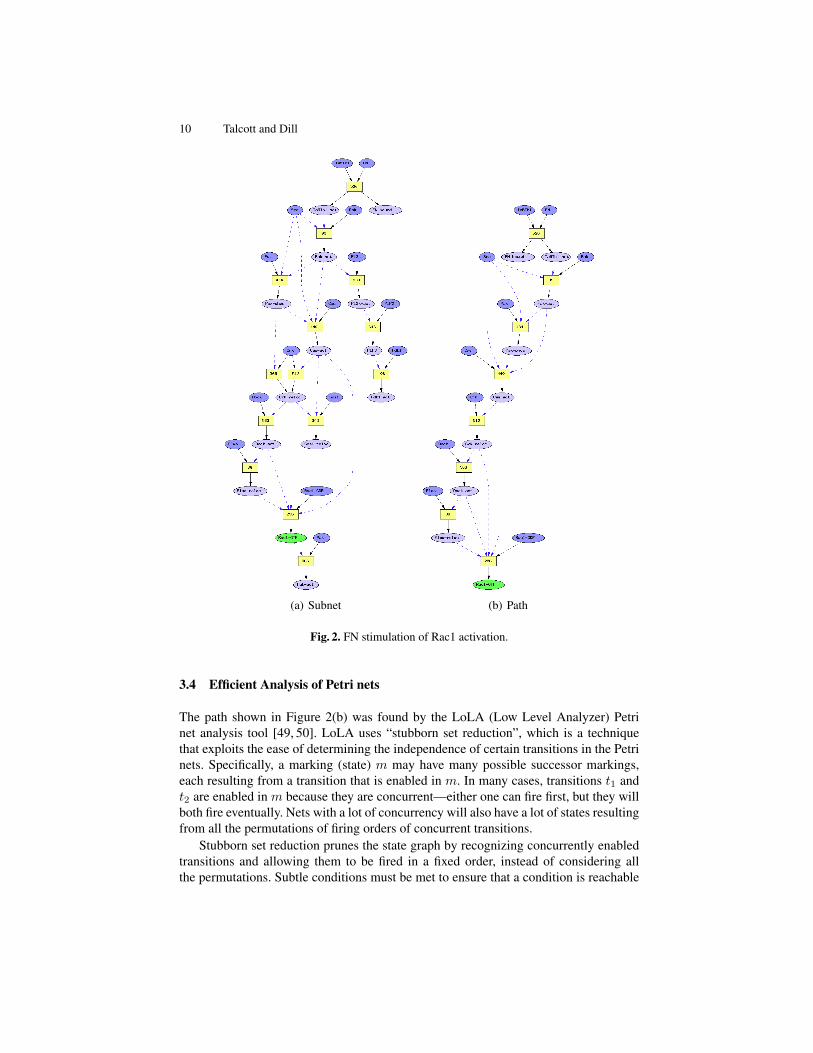
an avoid. Petri subnets are generated by a ‘relevant subnet’ computation that simplifiesthe specified analysis problem. Although a Petri subnet is a Petri net, it is only equiva-lent to the original net for a goal set that is a subset ofG or an avoid set that is a supersetof A. For example, for a goal that is not in G there may be a path in the original net, butnot in the subnet, since transitions needed for this goal may have been discarded as notbeing relevant. Figure 2(a) shows the relevant subnet of the Rac1 activation model whenthe goal is activation of Rac1, avoiding activation of EGFR (Maude property racAct3

in Example 1 of §3.2).

Computations are data structures used to represent system executions. We model acomputation as a sequence of steps, each step being a triple consisting of a source state,a rule instance or transition that applies to that state, and a target state, the state resultingfrom the rule application. The target state of the ith step of a computation must be equalto the source state of the i+ 1st step. A compact representation of a computation is thePetri net consisting of the initial state together with the set of rule instances occurringas computation steps. We call this net a path. Figure 2(b) shows a path in the subnet ofFigure 2(a). It can be executed as follows: If all of the ovals connected to a box by anincoming arrow (solid or dashed) are colored dark then color the outputs dark and makethe inputs connected by solid arrows light color. Repeating this procedure, a state canbe reached with Rac1 activated (Rac1-GTP colored dark).

10 Talcott and Dill

(a) Subnet (b) Path

Fig. 2. FN stimulation of Rac1 activation.

3.4 Efficient Analysis of Petri nets

The path shown in Figure 2(b) was found by the LoLA (Low Level Analyzer) Petrinet analysis tool [49, 50]. LoLA uses “stubborn set reduction”, which is a techniquethat exploits the ease of determining the independence of certain transitions in the Petrinets. Specifically, a marking (state) m may have many possible successor markings,each resulting from a transition that is enabled in m. In many cases, transitions t1 andt2 are enabled in m because they are concurrent—either one can fire first, but they willboth fire eventually. Nets with a lot of concurrency will also have a lot of states resultingfrom all the permutations of firing orders of concurrent transitions.

Stubborn set reduction prunes the state graph by recognizing concurrently enabledtransitions and allowing them to be fired in a fixed order, instead of considering allthe permutations. Subtle conditions must be met to ensure that a condition is reachable


in the reduced graph if and only if it is reachable in the original graph (the reader isreferred to [51]). For highly concurrent graphs, stubborn set reduction can acceleratethe solution of the reachability problem by many orders of magnitude.

For reachability queries on Pathway Logic nets, answering a reachability query thatwould have taken hours using a general purpose model-checking tool takes on the orderof a second in LoLA—fast enough to permit interactive use. As an example, LoLA wasrun on 5 examples, with and without the stubborn set reduction option turned on. Theexamples were 5 queries on a single Petri net, each causing exploration of a differentpart of the network. The experiments were conducted on a an IBM ThinkPad X22 withan 800 MHz Pentium III CPU and 256 MB of RAM. All the examples completed withina fraction of a second with stubborn set reduction turned on. With stubborn set reductionturned off 4 of the examples completed within a fraction of a second. The 5th examplewas stopped after 28.5 minutes. At this point LoLA had generated 2,495,854 states,traversed 35,400,000 edges, and was using 500 MB of virtual memory, and all 256MBof physical memory.

In our experience, these results are typical. Without stubborn set reduction, LoLAeither finishes quickly or runs for a very long time. With stubborn set reduction, it veryreliably finishes in a fraction of a second on the many examples we have tried.

It is beyond the scope of this paper to compare different model-checking tools forPathway Logic models. The interested reader can find such a comparison in [52]. Wenote that for the goals and avoids type queries, LoLA’s performance is by far the best.

4 Relating PLMaude and Petri Nets

It is well known that Petri nets can be represented in rewriting logic [48]. The variousforms that PLMaude models have taken as the modeling ideas have matured have led usto identify a special class of rewrite theories, called occurrence-based rewrite theories,that, restricted to terms reachable from a given initial term, have a natural representa-tion as Petri nets. The idea is to build on the equivalence of the dish and occurrencesrepresentations of states and to identify the features of PLMaude models needed toensure that the translation to the Petri net formalism preserves computations and goals-avoids properties. Furthermore, the resulting Petri net models can be transformed backinto rewriting logic, again preserving computations and goals-avoids properties. In thissection we define the mappings between PLMaude and Petri net models and the subnetreduction, and sketch proofs of correctness. These mappings are implemented in Maudeand used in PLA.

4.1 Some rewriting logic notation

We first introduce some notation for talking about rewrite theories. A rewrite theory,R, is a triple ((Σ,E ),R) where (Σ,E ) is an equational theory (for example, in ordersorted logic) with sorts and operations given by Σ and equations E , and R is a set ofrules of the form (t0 ⇒ t1 if c) where t0, t1 are terms, the rule premise and conclusionrespectively, and c is a boolean term, the rule condition. Viewing PLMaude as a rewrite

12 Talcott and Dill

theory, (Σ,E ) is given by the first two layers (sorts and operations, components) andR is given by the rules layer.

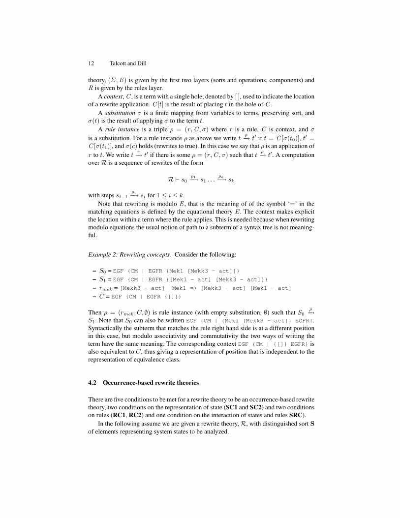
A context, C , is a term with a single hole, denoted by [ ], used to indicate the locationof a rewrite application. C [t] is the result of placing t in the hole of C .

A substitution σ is a finite mapping from variables to terms, preserving sort, andσ(t) is the result of applying σ to the term t.

A rule instance is a triple ρ = (r ,C , σ) where r is a rule, C is context, and σis a substitution. For a rule instance ρ as above we write t

ρ−→ t′ if t = C [σ(t0)], t′ =C [σ(t1)], and σ(c) holds (rewrites to true). In this case we say that ρ is an application ofr to t. We write t r−→ t′ if there is some ρ = (r ,C , σ) such that t

ρ−→ t′. A computationover R is a sequence of rewrites of the form

R ` s0ρ1−→ s1 . . .

ρk−→ sk

with steps si−1ρi−→ si for 1 ≤ i ≤ k.

Note that rewriting is modulo E , that is the meaning of of the symbol ‘=’ in thematching equations is defined by the equational theory E . The context makes explicitthe location within a term where the rule applies. This is needed because when rewritingmodulo equations the usual notion of path to a subterm of a syntax tree is not meaning-ful.

Example 2: Rewriting concepts. Consider the following:

– S0 = EGF {CM | EGFR {Mek1 [Mekk3 - act]}}

– S1 = EGF {CM | EGFR {[Mek1 - act] [Mekk3 - act]}}

– rmek = [Mekk3 - act] Mek1 => [Mekk3 - act] [Mek1 - act]

– C = EGF {CM | EGFR {[]}}

Then ρ = (rmek, C, ∅) is rule instance (with empty substitution, ∅) such that S0ρ−→

S1. Note that S0 can also be written EGF {CM | {Mek1 [Mekk3 - act]} EGFR}.Syntactically the subterm that matches the rule right hand side is at a different positionin this case, but modulo associativity and commutativity the two ways of writing theterm have the same meaning. The corresponding context EGF {CM | {[]} EGFR} isalso equivalent to C, thus giving a representation of position that is independent to therepresentation of equivalence class.

4.2 Occurrence-based rewrite theories

There are five conditions to be met for a rewrite theory to be an occurrence-based rewritetheory, two conditions on the representation of state (SC1 and SC2) and two conditionson rules (RC1, RC2) and one condition on the interaction of states and rules SRC).

In the following assume we are given a rewrite theory, R, with distinguished sort Sof elements representing system states to be analyzed.


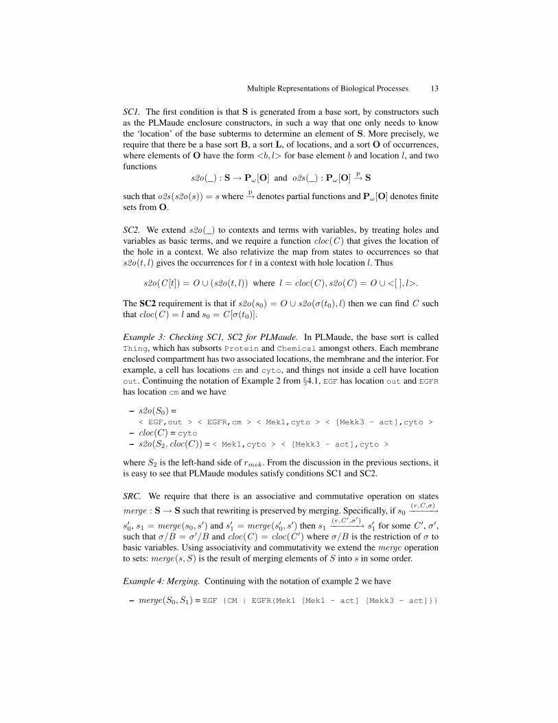
SC1. The first condition is that S is generated from a base sort, by constructors suchas the PLMaude enclosure constructors, in such a way that one only needs to knowthe ‘location’ of the base subterms to determine an element of S. More precisely, werequire that there be a base sort B, a sort L, of locations, and a sort O of occurrences,where elements of O have the form <b, l> for base element b and location l, and twofunctions

s2o(_) : S → Pω[O] and o2s(_) : Pω[O]p→ S

such that o2s(s2o(s)) = s wherep→ denotes partial functions and Pω[O] denotes finite

sets from O.

SC2. We extend s2o(_) to contexts and terms with variables, by treating holes andvariables as basic terms, and we require a function cloc(C ) that gives the location ofthe hole in a context. We also relativize the map from states to occurrences so thats2o(t, l) gives the occurrences for t in a context with hole location l. Thus

s2o(C [t]) = O ∪ (s2o(t, l)) where l = cloc(C ), s2o(C ) = O ∪<[ ], l>.

The SC2 requirement is that if s2o(s0) = O ∪ s2o(σ(t0), l) then we can find C suchthat cloc(C ) = l and s0 = C [σ(t0)].

Example 3: Checking SC1, SC2 for PLMaude. In PLMaude, the base sort is calledThing, which has subsorts Protein and Chemical amongst others. Each membraneenclosed compartment has two associated locations, the membrane and the interior. Forexample, a cell has locations cm and cyto, and things not inside a cell have locationout. Continuing the notation of Example 2 from §4.1, EGF has location out and EGFR

has location cm and we have

– s2o(S0) =< EGF,out > < EGFR,cm > < Mek1,cyto > < [Mekk3 - act],cyto >

– cloc(C) = cyto

– s2o(S2, cloc(C)) = < Mek1,cyto > < [Mekk3 - act],cyto >

where S2 is the left-hand side of rmek. From the discussion in the previous sections, itis easy to see that PLMaude modules satisfy conditions SC1 and SC2.

SRC. We require that there is an associative and commutative operation on states

merge : S → S such that rewriting is preserved by merging. Specifically, if s0(r ,C ,σ)−−−−−→

s′0, s1 = merge(s0, s′) and s′1 = merge(s′0, s′) then s1

(r ,C ′,σ′)−−−−−−→ s′1 for some C ′, σ′,such that σ/B = σ′/B and cloc(C ) = cloc(C ′) where σ/B is the restriction of σ tobasic variables. Using associativity and commutativity we extend the merge operationto sets: merge(s, S) is the result of merging elements of S into s in some order.

Example 4: Merging. Continuing with the notation of example 2 we have

– merge(S0, S1) = EGF {CM | EGFR{Mek1 [Mek1 - act] [Mekk3 - act]}}

14 Talcott and Dill

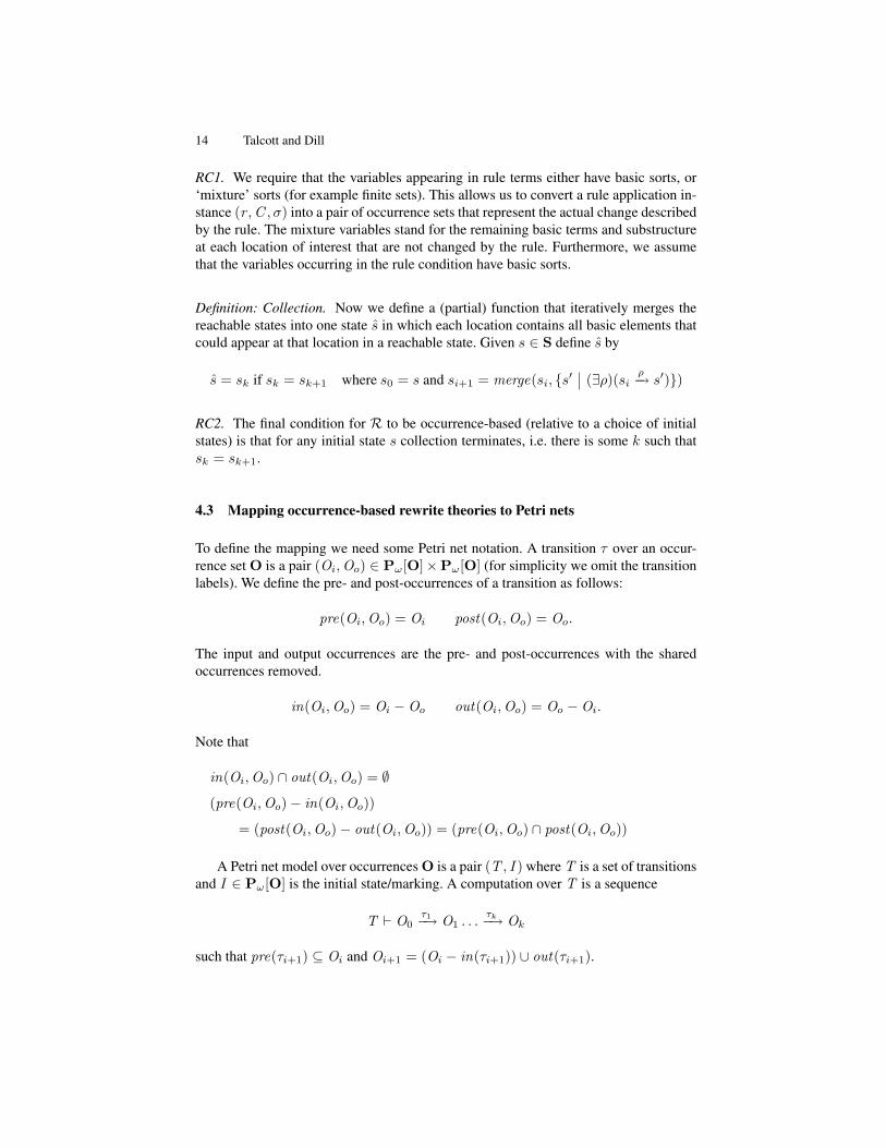
RC1. We require that the variables appearing in rule terms either have basic sorts, or‘mixture’ sorts (for example finite sets). This allows us to convert a rule application in-stance (r ,C , σ) into a pair of occurrence sets that represent the actual change describedby the rule. The mixture variables stand for the remaining basic terms and substructureat each location of interest that are not changed by the rule. Furthermore, we assumethat the variables occurring in the rule condition have basic sorts.

Definition: Collection. Now we define a (partial) function that iteratively merges thereachable states into one state s in which each location contains all basic elements thatcould appear at that location in a reachable state. Given s ∈ S define s by

s = sk if sk = sk+1 where s0 = s and si+1 = merge(si, {s′ (∃ρ)(siρ−→ s′)})

RC2. The final condition for R to be occurrence-based (relative to a choice of initialstates) is that for any initial state s collection terminates, i.e. there is some k such thatsk = sk+1.

4.3 Mapping occurrence-based rewrite theories to Petri nets

To define the mapping we need some Petri net notation. A transition τ over an occur-rence set O is a pair (Oi,Oo) ∈ Pω[O]×Pω[O] (for simplicity we omit the transitionlabels). We define the pre- and post-occurrences of a transition as follows:

pre(Oi,Oo) = Oi post(Oi,Oo) = Oo.

The input and output occurrences are the pre- and post-occurrences with the sharedoccurrences removed.

in(Oi,Oo) = Oi −Oo out(Oi,Oo) = Oo −Oi.

Note that

in(Oi,Oo) ∩ out(Oi,Oo) = ∅

(pre(Oi,Oo)− in(Oi,Oo))

= (post(Oi,Oo)− out(Oi,Oo)) = (pre(Oi,Oo) ∩ post(Oi,Oo))

A Petri net model over occurrences O is a pair (T , I ) where T is a set of transitionsand I ∈ Pω[O] is the initial state/marking. A computation over T is a sequence

T ` O0τ1−→ O1 . . .

τk−→ Ok

such that pre(τi+1) ⊆ Oi and Oi+1 = (Oi − in(τi+1)) ∪ out(τi+1).


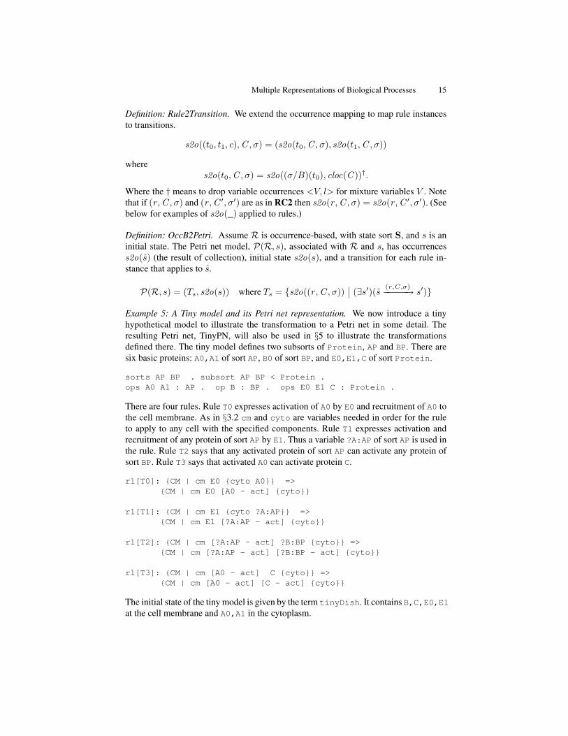
Definition: Rule2Transition. We extend the occurrence mapping to map rule instancesto transitions.

s2o((t0, t1, c),C , σ) = (s2o(t0,C , σ), s2o(t1,C , σ))

wheres2o(t0,C , σ) = s2o((σ/B)(t0), cloc(C ))†.

Where the † means to drop variable occurrences <V, l> for mixture variables V . Notethat if (r ,C , σ) and (r ,C ′, σ′) are as in RC2 then s2o(r ,C , σ) = s2o(r ,C ′, σ′). (Seebelow for examples of s2o(_) applied to rules.)

Definition: OccB2Petri. Assume R is occurrence-based, with state sort S, and s is aninitial state. The Petri net model, P(R, s), associated with R and s, has occurrencess2o(s) (the result of collection), initial state s2o(s), and a transition for each rule in-stance that applies to s.

P(R, s) = (Ts, s2o(s)) where Ts = {s2o((r ,C , σ)) (∃s′)(s (r ,C ,σ)−−−−−→ s′)}

Example 5: A Tiny model and its Petri net representation. We now introduce a tinyhypothetical model to illustrate the transformation to a Petri net in some detail. Theresulting Petri net, TinyPN, will also be used in §5 to illustrate the transformationsdefined there. The tiny model defines two subsorts of Protein, AP and BP. There aresix basic proteins: A0,A1 of sort AP, B0 of sort BP, and E0,E1,C of sort Protein.

sorts AP BP . subsort AP BP < Protein .ops A0 A1 : AP . op B : BP . ops E0 E1 C : Protein .

There are four rules. Rule T0 expresses activation of A0 by E0 and recruitment of A0 tothe cell membrane. As in §3.2 cm and cyto are variables needed in order for the ruleto apply to any cell with the specified components. Rule T1 expresses activation andrecruitment of any protein of sort AP by E1. Thus a variable ?A:AP of sort AP is used inthe rule. Rule T2 says that any activated protein of sort AP can activate any protein ofsort BP. Rule T3 says that activated A0 can activate protein C.

rl[T0]: {CM | cm E0 {cyto A0}} =>{CM | cm E0 [A0 - act] {cyto}}

rl[T1]: {CM | cm E1 {cyto ?A:AP}} =>{CM | cm E1 [?A:AP - act] {cyto}}

rl[T2]: {CM | cm [?A:AP - act] ?B:BP {cyto}} =>{CM | cm [?A:AP - act] [?B:BP - act] {cyto}}

rl[T3]: {CM | cm [A0 - act] C {cyto}} =>{CM | cm [A0 - act] [C - act] {cyto}}

The initial state of the tiny model is given by the term tinyDish. It contains B,C,E0,E1at the cell membrane and A0,A1 in the cytoplasm.

16 Talcott and Dill

tinyDish = PD({CM | B C E0 E1 {A0 A1}}) .

The collection starting with the dish tinyDish using the rules T0,T1,T2 yields thedish tinyDish*. Rule T0 adds [A0 - act] to the membrane compartment, rule T1

instantiated with ?A:AP as A1 adds [A1 - act] to the membrane compartment. Theinstantiation of rule T1 with ?A:AP as A0 adds nothing new. Rule T2 instantiated with?B:BP as B0 adds [B0 - act] to the membrane compartment. For the dish tinyDishthere is only one instantiation of rule T2. Rule T3 adds [C - act] to the membranecompartment.

tinyDish* = PD({CM | [A0 - act] [A1 - act] [B - act] BC [C -act] E0 E1{A0 A1}}) .

The Petri net TinyPN has transitions tinyT, obtained by applying s2o( ) to rule in-stances for tinyDish*, and occurrences tinyI, the result of s2o(tinyDish). Herewe added labels to the transitions for convenient reference. If there is more than onerule instance, the transition labels are indexed by instance numbers, just to keep labelsunique.

TinyPN = (tinyT,tinyI)tinyI = < B,cm >< C,cm >< E0,cm >< E1,cm >< A0,cyto >< A1,cyto >tinyT =

(T0, < E0,cm> < A0,cyto > => < E0,cm > < [A0 - act],cm >)(T1.0, < E1,cm> < A0,cyto > => < E1,cm > < [A0 - act],cm >)(T1.1, < E1,cm> < A1,cyto > => < E1,cm > < [A1 - act],cm >)(T2.0, < [A0 - act],cm >< B,cm > =>

< [A0 - act],cm >< [B - act],cm >(T2.1, < [A1 - act],cm >< B,cm > =>

< [A1 - act],cm >< [B - act],cm >(T3, < [A0 - act],cm >< C,cm > =>

< [A0 - act],cm >< [C - act],cm >

For example there are two instances of rule T1, ρ0 = ((t0, t1),C , σ0) and ρ1 =((t0, t1),C , σ1) where

– t0 = {CM | cm E1 {cyto ?A:AP}}– t1 = \{CM | cm E1 [?A:AP - act] \{cyto\}\}– C = PD([])– σ0/B binds ?A:AP to A0– σ1/B binds ?A:AP to A1

Using the rule for transforming instances to transitions we obtain the transition labeledT1.0 as follows.

s2o((t0, t1),C , σ0)

= (s2o((σ0/B)(t0), cloc(C )), s2o((σ0/B)(t1), cloc(C )))

= (s2o({CM | cm E1{cyto A0}}, out),s2o({CM | cm E1[A0 - act]{cyto}}, out))

= (< E1, cm >< A0,cyto >, < E1,cm >< [A0 - act],cm >)


Theorem: OccB2Petri. For R an occurrence-based rewrite theory and s an initial state,the mapping to Petri nets preserves computations. Specifically, if (Ts, s2o(s)) = P(R, s),then

R ` s = s0ρ1−→ s1 . . .

ρk−→ sk ⇔ Ts ` s2o(s0)s2o(ρ1)−−−−−→ s2o(s1) . . .

s2o(ρk)−−−−−→ s2o(sk).

Proof Sketch. By induction on the computation length k. If siρi+1−−−→ si+1 then

s2o(ρi+1) ∈ Ts by SRC. Let ρi+1 = (r ,C , σ) with r = (t0, t1, c) and l = cloc(C ).Then si = C [σ(t0)], si+1 = C [σ(t1)], and for some occurrence set O s2o(si) =

s2o(σ(t0), l)∪O and s2o(si+1) = s2o(σ(t1), l)∪O. Thus s2o(si)s2o(ρi+1)−−−−−−→ s2o(si+1).

Conversely, let Oiτi+1−−−→ Oi+1, and by induction Oi = s2o(si) for some reachable si.

Also τ = (O0,O1) = s2o(r ,C , σ) where (r ,C , σ) applies to s. We can find O′

such that Oi = O′ ∪ O0 and Oi+1 = O′ ∪ O1. By SC3 we can find C ′, σ′ such that

si = C ′[σ′(t0)], and si(r ,C ′,σ′)−−−−−−→ si+1 where s2o(si+1) = Oi+1.

Counterexample. To see that requirement (SRC) that merging preserves rewrites isneeded, consider the following rule variants in the Pathway Logic language:

[r1]: {CM | Ras {cyto Rac}} => {CM | Ras [Rac - act]{cyto}}[r2]: {CM | cm Ras {cyto Rac}} => {CM | cm Ras [Rac - act]{cyto}}

where cyto and cm are variables standing for any other components located in the cyto-plasm or cell membrane respectively. Consider the state {CM | Ras Grb2 {Src Rac}}

which can be obtained from {CM | Ras {Src Rac}} by a merge. The rule r2 ap-plies but r1 does not, although r1 applies to the ‘before merge’ state. Both rules trans-form to the same Petri net transition:

< Ras,CM > < Rac,Cyto > => < Ras,CM > < [Rac - act],CM >

which indeed applies to the corresponding occurrence state

< Ras,cm > < Grb2,cm >< Rac,cyto > < Src,cyto >

Definition: Petri2RWL. The conversion of an occurrence Petri net to a rewrite theoryis simple. If (Ts, s2o(s)) = P(R, s), then PS(R, s) is the rewrite theory with theequational part of R extended with the definition of occurrences, and rules

{Oi ⇒ Oo (Oi,Oo) ∈ Ts}

Theorem: Petri2RWL. The mapping PS preserves computations.

PS(R, s) ` s2o(s) τ1−→ . . .τk−→ Ok ⇔ Ts ` s2o(s) τ1−→ . . .

τk−→ Ok

18 Talcott and Dill

5 Relating and transforming queries

5.1 Preservation of properties

The temporal logic used by the Maude model checker, LTL, is based on atomic propo-sitions that can be defined by boolean functions in Maude. In the case of an occurrence-based rewrite theory, we restrict attention to propositions that are positive (goals) andnegative (avoids) occurrence tests – basic component b occurs (or does not occur) atlocation l. These propositions translate to simple membership tests <b, l> ∈ s2o(s) inthe corresponding Petri net model. For example, the property racAct3 presented in Ex-ample 1 of §3.2 contains one positive occurrence test (for the presence of < [Rac1 -

GTP], cm >) and one negative occurrence test (for the absence of < [EGFR - act],

cm >).Let LTLO be the Maude LTL language with propositional part restricted to occur-

rence propositions. Let ψ be an LTLO formula expressed in the PLMaude language andlet s2o(ψ) be the same property expressed in terms of occurrence membership, liftings2o(_) homomorphically (on syntax) to LTLO formulas.

Theorem: LTLO. Given an occurrence-based rewrite theory R and initial state s, let πbe a computation of R, s, π′ be the corresponding computation of P(R, s), and π′′ bethe corresponding computation of PS(R, s). Then for any LTLO formula ψ

π |= ψ ⇔ π′ |= s2o(ψ) ⇔ π′′ |= s2o(ψ)

and thus

(R, s) |= ψ ⇔ P(R, s) |= s2o(ψ) ⇔ (PS(R, s), s) |= s2o(ψ)

This is a consequence of the isomorphism of computations and the preservation ofsatisfaction of occurrence properties by the occurrence translations.

Note that the LTLO theorem implies that counterexamples are also preserved. Thisis important, since queries asking to find a computation having certain properties areanswered by asking a model-checker to find a counterexample to the assertion that nosuch computation exists.

5.2 Relevant Subnets for Goals-Avoids Queries

As indicated in § 3, we are especially interested in answering queries of the form “giveninitial state I , find a path that satisfies (G,A)” where (G,A) is a basic goals-avoidsproperty with goals G and avoids A. We interpret this as meaning find a path (that is, acomputation) starting with the initial state I , that reaches a state satisfying goals G, andsuch that no state in the path contains any occurrence of A. Without loss, we furtherrequire the path to be minimal, in the sense of not using irrelevant transitions. That is,if any transition is removed from the set generating the path, the remaining transitionsdo not generate a path satisfying the goals. Ideally we would like to focus attention onthe subnet of transitions of a Petri net model that might appear in any minimal pathsatisfying that property. We call these the truly relevant transitions. This is of interest


both to help the biologist focus on a smaller set of transitions and to reduce the searchspace to be considered by an analysis tool.

Finding just the truly relevant transitions means finding exactly the minimal pathssatisfying a given property, the problem we are trying to simplify. Thus we will lookfor a safe approximation, called the relevant transitions, that is a superset of truly rel-evant transitions set. Clearly, transitions that mention an occurrence to be avoided canbe eliminated, as can transitions that do not contribute to reaching some goal, or transi-tions whose pre-set will not be a subset of a reachable state. In the following we definethree transformations that formalize these intuitions. The first transformation removestransitions that mention an occurrence to be avoided. The second transformation is abackwards collection of transitions that contribute to reaching a goal, either becausethe post-occurrences contain a goal, or recursively contain a pre-occurrence of somecontributing transition. The third transformation is a forward collection of transitionsapplicable to reachable states. Then given a Petri net (T , I ), and a goals-avoids prop-erty (G ,A), T is transformed/reduced to the corresponding set of relevant transitionsrelTrans(T , I ,G ,A) by the following process:

A G I↓ avoids ↓ backwards ↓ forwards

[T ] −→ [T/A] −→ [(T/A)bG] −→ [((T/A)b

G)fI ]

elimination collection collection

We will show that any minimal path from initial state I meeting a goals-avoids property(G ,A) using transitions in T , in fact uses only transitions in relTrans(T , I ,G ,A),thus it is a safe approximation.

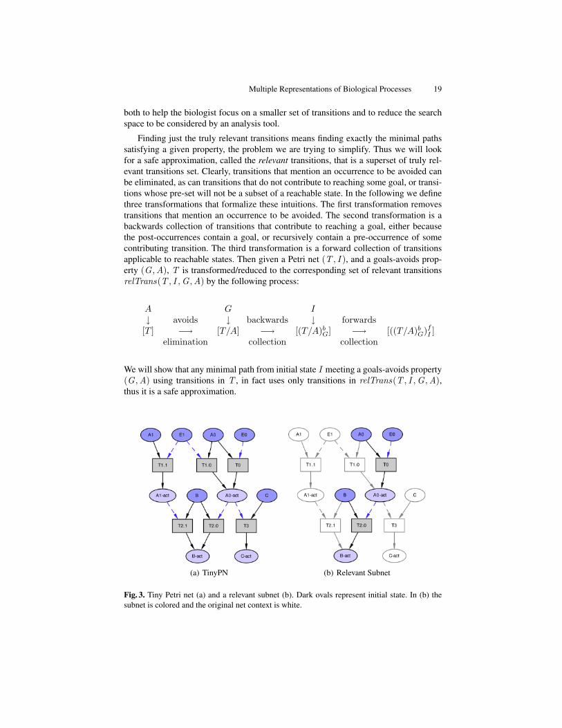
(a) TinyPN (b) Relevant Subnet

Fig. 3. Tiny Petri net (a) and a relevant subnet (b). Dark ovals represent initial state. In (b) thesubnet is colored and the original net context is white.

20 Talcott and Dill

Figure 3 show the Petri net tinyPN = (tinyT, tinyI) from Example 5 of §4.3. In thegraphical form we use simple names to label (and refer to) occurrences, leaving thelocation part implicit. This will be used to illustrate the concepts and transformationsdiscussed below.

Definition: Minimal Paths. Let I (initial state), G (goals), A (avoids) be occurrence setssuch that (I ∪G) ∩A = ∅. The set P(T , I ,G ,A) is the set of Petri net computations,π, that start from the initial state I , and reach a state containing all occurrences in G ,using transitions in T without ever marking A.

π = O0τ1−→ . . .

τk−→ Ok ∈ P(T , I ,G ,A) ⇔ O0 = I ∧G ⊆ Ok ∧∧

0≤i≤k

Oi∩A = ∅

π is minimal if there is no computation π′ in P(T , I ,G ,A) that uses a proper subsetof the transitions used in π, and we let mP(T , I ,G ,A) be the set of computations ofP(T , I ,G ,A) that are minimal.

Example 6: Minimal and non Minimal Paths. In tinyPN (Figure 3) the transitionsT1.1, T1.0 form a path to the goal A0-act, but it is not minimal as T1.1 can beremoved since T1.0 alone is a path.

Lemma: Path Monotonicity. The set of minimal paths monotonically increases withincreasing initial state and decreasing goals and avoids. Specifically, if T ⊆ T ′, I ⊆ I ′,G ′ ⊆ G , A′ ⊆ A, then

P(T , I ,G ,A) ⊆ P(T ′, I ′,G ′,A′)

and

mP(T , I ,G ,A) ⊆ mP(T ′, I ′,G ′,A′)

Definition: Removing Avoids. Assume given T and A as above. The result of removingrules that mention an element of A is defined by

T/A = {τ ∈ T (pre(τ) ∪ post(τ)) ∩A = ∅}

Example 7. Removing Avoids. Taking A to be A1*, removing the avoids from the tran-sitions of tinyPN means removing T1.1 and T2.1, leaving T0, T1.0, T2.0, and T3,that is

tinyT/A = {T0, T1.0, T2.0, T3}.

Lemma: Removing Avoids is Safe. If π ∈ mP(T , I ,G ,A), then π ∈ mP(T/A, I ,G ,A).Proof. Since by definition no transition in T − T/A could be used in π.


Definition: Backward collection. Assume given T , G as above. The backward collec-tion T b

G of T relative to G is defined by

T bG =

⋃j∈Nat

T bj where

G0 = G Gj+1 = Gj ∪⋃

τ∈Tbj

pre(τ)

T bj = {τ ∈ T out(τ) ∩Gj 6= ∅}

Note that for some n, Gj = Gj+1 for j > n since T is finite and thus only finitelymany increments can be made.

Example 8. Backwards Collection. Backwards collection of tinyT for goal B-act,tinyTb

B-act, is tinyT minus T3. The can be seen from the following steps in thecollection:

G0 = B-act

tinyTb0 = {T2.0, T2.1}

G1 = {B-act, B, A0-act, A1-act}

tinyTb0 = tinyTb

0 ∪ {T0, T1.0, T1.1}

As another example, for goals A0-act and A1-act we have

tinyTb{A0-act,A1-act} = {T0, T1.0, T1.1}

Lemma: Backward Monotonicity. Backwards collection is monotonic in transitions andgoals. That is, if T ⊆ T ′ and G ⊆ G ′, then T b

G ⊆ (T ′)bG′ .

The lemma Backwards 1 captures the essence of the reason that a transition thatappears in some minimal path for a set of goals is one produced by backwards collec-tion.

Lemma: Backwards 1. If O τ1−→ O1τ2−→ O2 and pre(τ2)∩out(τ1) = ∅ then we can find

O ′2 such that O τ2−→ O ′

2. Furthermore, for any occurrence set G∗, if out(τ1) ∩G∗ = ∅,then G∗ ∩O2 ⊆ G∗ ∩O ′

2.Proof. With the assumptions of the lemma, pre(τ2) ⊆ O , letting O ′

2 = (O− in(τ2))∪out(τ2) we have, by definition of transition, the desired transition. Also by definition oftransition, O2 = ((O−in(τ1)∪out(τ1))−in(τ2))∪out(τ2). Assuming out(τ1)∩G∗ =∅ we have G∗ ∩O2 = G∗ ∩ ((O − in(τ1)− in(τ2)) ∪ out(τ2)) ⊆ G∗ ∩O ′

2.The lemma Backwards 2 identifies conditions under which a sequence of transi-

tions can be restarted at a new state. For backwards collection, the state of interest isone resulting from deleting an irrelevant transition, such as τ1 in Backwards 1.

22 Talcott and Dill

Lemma: Backwards 2. If O ∩ G ⊆ O ′ ∩ G , pre(τ) ⊆ G and O τ−→ O1, then we canfind O ′

1 such that O1 ∩G ⊆ O ′1 ∩G and O ′ τ−→ O ′

1.Proof. By the assumptions, pre(τ) ⊆ O ′, so letting O ′

1 = (O ′ − in(τ)) ∪ out(τ)we have the desired transition. Since O1 = (O − in(τ)) ∪ out(τ), if g ∈ O1 eitherg ∈ out(τ) or g ∈ O − in(τ) ⊆ O ′ − in(τ). Thus g ∈ O ′

1.

Theorem: Backward safety. If π ∈ mP(T , I ,G ,A), then π ∈ mP(T bG , I ,G ,A).

Proof Sketch. Let π = I τ1−→ O1 . . .τk−→ Ok ∈ mP(T , I ,G ,A). We show that

τj ∈ T bG for 1 ≤ j ≤ k. Suppose not. Let G∗ be the union of the Gjs in the definition

of T bG , and let j be the largest number such that τj 6∈ T b

G . Thus out(τj) ∩ G∗ = ∅.We construct π′ ∈ P(T , I ,G ,A) using fewer transitions, contradicting minimalityof π. If j = k then G ⊆ Ok−1 and π′ is the first k − 1 transitions of π. If j < kthen let O ′

j = Oj−1, and O ′i+1 = (O ′

i − in(τi+1)) ∪ out(τi+1) for j ≤ i < k. Bymaximality of j, τi+1 ∈ T b

G and thus pre(τi+1) ⊆ G∗ for j ≤ i < k. We claim thatOi+1 ∩ G∗ ⊆ O ′

i+1 ∩ G∗ and O ′i

τi+1−−−→ O ′i+1 for j ≤ i < k. For i = j this follows

by backwards lemma 1 and for i > j it follows by backwards lemma 2. Thus takingπ′ = I τ1−→ O1 . . .

τj−1−−−→ O ′j

τj+1−−−→ . . .τk−→ O ′

k we are done.

Definition: Forward collection. The forward collection T fI of T relative to I is defined

by

T fI =

⋃j∈Nat

T fj I f =

⋃j∈Nat

Ij where

I0 = I Ij+1 =⋃

τ∈Tfj

post(τ)

T fj = {τ ∈ T pre(τ) ⊆ Ij}

Again, we have that for some n, Ij = In for j ≥ n.

Example 9. Forward Collection. Suppose we remove E1 from the inital state, callthis I1, then forward collection of tinyT from I1 omits T1.0, T1.1 and T2.1. ThustinyT

fI1

= {T0, T2.0, T3}.

Lemma: Forward Monotonicity. If T ⊆ T ′ and I ⊆ I ′, then T fI ⊆ (T ′)f

I ′

Theorem: Forward safety. If π ∈ mP(T , I ,G ,A), then π ∈ mP(T fI , I ,G ,A).

Proof. This is because for each transition τj+1 in π, using the notation of the definition,pre(τj+1) ⊆ Ij , and thus τj+1 ∈ T f

j for 0 ≤ j < k.

Definition: Relevant Subnet. The subnet of transitions from T relevant to initial stateI , goals G , and avoids A is defined by

relTrans(T , I ,G ,A) = ((T/A)bG)f

I .


Corollary: Relevant Subnet. If π ∈ mP(T , I ,G ,A) is non-empty, then

π ∈ mP(relTrans(T , I ,G ,A), I ,G ,A)

Thus search for such paths can be carried out in the relevant subnet relTrans(T , I ,G ,A).Note that if G 6⊆ I f then P(T , I ,G ,A) is empty.

Example 10. Relevant subnets. The relevant subnet of tinyPN for goals B-act, avoidsA1-act and initial state I1 = tinyI− E1

relTrans(tinyT, I1, B-act, A1-act) = {T0, T2.0}

is shown in figure 3(b).

6 Summary and Future Work

The main contributions of the paper are: a definition of mappings between rewritinglogic and petri net representations of biological processes (and similar concurrent pro-cesses) that satisfy certain conditions; proof that these mappings preserve properties ofinterest; and definition of a relevant subnet transformation that reduces the number oftransitions that must be considered in search for a path satisfying a goals-avoids prop-erty.

As context we presented an overview of Pathway Logic illustrated with a model ofRac1 activation as Maude rules and the representation as a Petri net. We also discussthe advantages of analyses based on Petri nets.

As models grow in size, we expect to need to explore alternative path finding algo-rithms. Possibilities include employing more highly tuned model checkers, discoveringnew simplification and abstraction transformations, and developing constraint solvingapproaches to take advantage of the rapid advances being made in this area. Anotherbig challenge is refining PLMaude models to incorporate semi-quantitative informationabout expression levels and relative preference for competing reactions, and to be ablecompute with and visualize the refined models in ways that are meaningful to workingbiologists.

Acknowledgments. The authors would like to thank the Pathway Logic team andthe anonymous reviewers for helpful criticisms. The work was partially funded byNIH/NIGMS grant GM68146.

References

1. Eker, S., Knapp, M., Laderoute, K., Lincoln, P., Meseguer, J., Sonmez, K.: Pathway Logic:Symbolic analysis of biological signaling. In: Proceedings of the Pacific Symposium onBiocomputing. (2002) 400–412

2. Eker, S., Knapp, M., Laderoute, K., Lincoln, P., Talcott, C.: Pathway Logic: Executablemodels of biological networks. In: Fourth International Workshop on Rewriting Logic and ItsApplications (WRLA’2002), Pisa, Italy, September 19 — 21, 2002. Volume 71 of ElectronicNotes in Theoretical Computer Science., Elsevier (2002) http://www.elsevier.nl/locate/entcs/volume71.html.

24 Talcott and Dill

3. Talcott, C., Eker, S., Knapp, M., Lincoln, P., Laderoute, K.: Pathway logic modeling ofprotein functional domains in signal transduction. In: Proceedings of the Pacific Symposiumon Biocomputing. (2004)

4. Clavel, M., Duran, F., Eker, S., Lincoln, P., Marti-Oliet, N., Meseguer, J., Talcott, C.: Maude2.0 Manual (2003) http://maude.cs.uiuc.edu.

5. Clavel, M., Duran, F., Eker, S., Lincoln, P., Martı-Oliet, N., Meseguer, J., Talcott, C.L.: TheMaude 2.0 system. In Nieuwenhuis, R., ed.: Rewriting Techniques and Applications (RTA2003). Volume 2706 of Lecture Notes in Computer Science., Springer-Verlag (2003) 76–87

6. Mason, I.A., Talcott, C.L.: IOP: The InterOperability Platform & IMaude: An interactive ex-tension of Maude. In: Fifth International Workshop on Rewriting Logic and Its Applications(WRLA’2004). Electronic Notes in Theoretical Computer Science, Elsevier (2004)

7. Kohn, K.W.: Functional capabilities of molecular network components controlling the mam-malian g1/s cell cycle phase transition. Oncogene 16 (1998) 1065–1075

8. Weng, G., Bhalla, U.S., Iyengar, R.: Complexity in biological signaling systems. Science284 (1999) 92–96

9. Shvartsman, S.Y., Hagan, M.P., Yacoub, A., Dent, P., Wiley, H., Lauffenburger, D.: Autocrineloops with positive feedback enable context-dependent cell signaling. Am J Physiol CellPhysiol 282 (2002) C545–559

10. Smolen, P., Baxter, D.A., Byrne, J.: Mathematical modeling of gene networks. Neuron 26(2000) 567–580

11. Lok, L.: Software for signaling networks, electronic and cellular. Science STKE PE11(2002)

12. Rao, C.V., Wolf, D.M., Arkin, A.P.: Control, exploitation and tolerance of intracellular noise.Nature 420 (2002) 231–237

13. Endy, D., Brent, R.: Modelling cellular behaviour. Nature 409 (2001) 391–39514. Peterson, J.L.: Petri Nets: Properties, analysis, and applications. Prentice-Hall (1981)15. Milner, R.: A Calculus of Communicating Systems. Springer Verlag (1980)16. Harel, D.: Statecharts: A visual formalism for complex systems. Science of Computer

Programming 8 (1987) 231–27417. Meseguer, J.: Conditional Rewriting Logic as a unified model of concurrency. Theoretical

Computer Science 96(1) (1992) 73–15518. Croes, D., Couche, F., van Helden, J., Wodak, S.: Path finding in metabolic networks: mea-

suring functional distances between enzymes. In: Open Days in Biology, Computer Scienceand Mathematics JOBIM 2004. (2004)

19. Hofestadt, R.: A Petri net application to model metabolic processes. Syst. Anal. Mod. Simul.16 (1994) 113–122

20. Reddy, V.N., Liebmann, M.N., Mavrovouniotis, M.L.: Qualitative analysis of biochemicalreaction systems. Comput. Biol. Med. 26 (1996) 9–24

21. Goss, P.J., Peccoud, J.: Quantitative modeling of stochastic systems in molecular biologyusing stochastic Petri nets. Proc. Natl. Acad. Sci. U. S. A. 95 (1998) 6750–6755

22. Kuffner, R., Zimmer, R., Lengauer, T.: Pathway analysis in metabolic databases via differ-ential metabolic display (DMD). Bioinformatics 16 (2000) 825–836

23. Matsuno, H., Doi, A., Nagasaki, M., Miyano, S.: Hybrid Petri net representation of generegulatory network. In: Pacific Symposium on Biocomputing. Volume 5. (2000) 341–352

24. Oliveira, J.S., Bailey, C.G., Jones-Oliveira, J.B., Dixon, D.A., Gull, D.W., Chandler, M.L.:An algebraic-combinatorial model for the identification and mapping of biochemical path-ways. Bull. Math. Biol. 63 (2001) 1163–1196

25. Genrich, H., Kuffner, R., Voss, K.: Executable Petri net models for the analysis of metabolicpathways. Int. J. STTT 3 (2001)


26. Oliveira, J.S., Bailey, C.G., Jones-Oliveira, J.B., Dixon, D.A., Gull, D.W., Chandler, M.L.:A computational model for the identification of biochemical pathways in the Krebs cycle. J.Computational Biology 10 (2003) 57–82

27. Zevedei-Oancea, I., Schuster, S.: Topological analysis of metabolic networks based on Petrinet theory. In Silico Biology 3(0029) (2003)

28. Regev, A., Silverman, W., Shapiro, E.: Representation and simulation of biochemical pro-cesses using the pi-calculus process algebra. In Altman, R.B., Dunker, A.K., Hunter, L.,Klein, T.E., eds.: Pacific Symposium on Biocomputing. Volume 6., World Scientific Press(2001) 459–470

29. Priami, C., Regev, A., Shapiro, E., Silverman, W.: Application of a stochastic name-passingcalculus to representation and simulation of molecular processes. Information ProcessingLetters (2001) in press.

30. Calder, M., Vyshemirsky, V., Gilbert, D., Orton, R.: Analysis of signalling pathways us-ing the PRISM model checker. In Plotkin, G., ed.: Proceedings of the Third InternationalConference on Computational Methods in System Biology (CMSB 2005). (2005)

31. Regev, A., Panina, E., Silverman, W., Cardelli, L., Shaprio, E.: Bioambients: An abstractionfor biological compartments (2003) to appear TCS.

32. Nielson, F., Nielson, H.R., Priami, C., Rosa, D.: Control flow analysis for bioambients. In:BioConcur. (2003)

33. Kam, N., Cohen, I., Harel, D.: The immune system as a reactive system: Modeling t cellactivation with statecharts. In: Proc. Visual Languages and Formal Methods (VLFM’01).(2001) 15–22

34. Efroni, S., Harel, D., Cohen, I.: Towards rigorous comprehension of biological complexity:Modeling, execution and visualization of thymic t-cell maturation. Genome Research (2003)Special issue on Systems Biology, in press.

35. Damm, W., Harel, D.: Breathing life into message sequence charts. Formal Methods inSystem Design 19(1) (2001)

36. Kam, N., Harel, D., Kugler, H., Marelly, R., Pnueli, A., Hubbard, J., Stern, M.: Formalmodeling of C.elegans development: A scenario-based approach. In: First InternationalWorkshop on Computational Methods in Systems Biology. Volume 2602 of Lecture Notesin Computer Science., Springer (2003) 4–20

37. Prez-Jimnez, M., Romero-Campero, F.: Modelling EGFR signalling cascade using continu-ous membrane systems. In Plotkin, G., ed.: Proceedings of the Third International Confer-ence on Computational Methods in System Biology (CMSB 2005). (2005)

38. Fages, F., Soliman, S., Chabrier-Rivier, N.: Modelling and querying interaction networks inthe biochemical abstract machine BIOCHAM. Journal of Biological Physics and Chemistry4(2) (2004) 64–73

39. Chabrier-Rivier, N., Chiaverini, M., Danos, V., Fages, F., Schachter, V.: Modeling and query-ing biomolecular interaction networks. Theoretical Computer Science 351(1) (2004) 24–44

40. Calzone, L., Chabrier-Rivier, N., Fages, F., Gentils, L., Soliman, S.: Machine learning bio-molecular interactions from temporal logic properties. In Plotkin, G., ed.: Proceedings ofthe Third International Conference on Computational Methods in System Biology (CMSB2005). (2005)

41. Baral, C., Chancellor, K., Tran, N., Tran, N., Joy, A., Berens, M.: A knowledge based ap-proach for representing and reasoning about signaling networks. Bioinformatics 20 (2004)i15–i22

42. Shankland, C., Tran, N., Baral, C., Kolch, W.: Reasoning about the ERK signal transductionpathway using BioSigNet-RR. In Plotkin, G., ed.: Proceedings of the Third InternationalConference on Computational Methods in System Biology (CMSB 2005). (2005)

26 Talcott and Dill

43. Hucka, M., Finney, A., Sauro, H., Bolouri, H., Doyle, J., Kitano, H.: The ERATO systemsbiology workbench: Enabling interaction and exchange between software tools for compu-tational biology. In: Proceedings of the Pacific Symposium on Biocomputing. (2002)

44. : BioSpice (2004) https://community.biospice.org/.45. : IBM Discoverylink (2004) http://publib-b.boulder.ibm.

com/Redbooks.nsf/0/3c7a635147cf20d785256a540064e287?OpenDocument&Highlight=0,DiscoveryLink.

46. : geneticXchange (2004) http://midas-10.cs.ndsu.nodak.edu/bio/ppts/chung.pdf.

47. Schmidt, A., Hall, A.: Guanine nucleotide exchange factors for rho gtpases: turning on theswitch. Genes Dev. 16 (2002) 1587–15609

48. Stehr, M.O.: A rewriting semantics for algebraic nets. In Girault, C., Valk, R., eds.: Petri Netsfor System Engineering – A Guide to Modelling, Verification, and Applications. Springer-Verlag (2000)

49. Schmidt, K.: LoLA: A Low Level Analyser. In Nielsen, M., Simpson, D., eds.: Applicationand Theory of Petri Nets, 21st International Conference (ICATPN 2000). Volume 1825 ofLecture Notes in Computer Science., Springer (2000) 465–474

50. : LoLA: Low Level Petri net Analyzer (2004) http://www.informatik.hu-berlin.de/∼kschmidt/lola.html.

51. Schmidt, K.: Stubborn sets for standard properties. In: International Conference on Applica-tion and Theory of Petri nets. Volume 1639 of Lecture Notes in Computer Science., Springer(1999) 46–65

52. Porter, D.: An Interpreter for JLambda (2004) http://mcs.une.edu.au/∼iop/Data/Papers/.

Documents

Multiple Representations of Biological Processes · 2006-07-16 · Multiple Representations of Biological Processes 3 There are many variants of the Petri net formalism and a variety