Embed Size (px)
Citation preview
Multiple timescale simulations of global macroscopic dynamics of magnetized plasma
Stephen C. Jardin1
N.M. Ferraro2, J. Breslau1, J. Chen1, 1Princeton Plasma Physics Laboratory
2 General Atomics
IPAM WorkshopComputational Challenges in Magnetized Plasma
University of California, Los AngelesApril 17, 2012
1
This work was performed in close collaboration with M. Shephard, F. Zhang, and F. Delalondre at the SCOREC center at Rensselaer Polytechnic Institute in Troy, NY.
Acknowledgements also to: G. Fu, S. Hudson, H. Strauss, L. Sugiyama
10-10 10-2 104100
SEC.
CURRENT DIFFUSION
10-8 10-6 10-4 102ωLH
-1Ωci
-1 τAΩce-1 ISLAND GROWTH
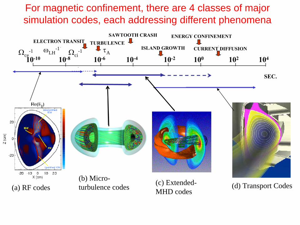
ENERGY CONFINEMENTSAWTOOTH CRASHTURBULENCEELECTRON TRANSIT
(a) RF codes(b) Micro-turbulence codes (c) Extended-
MHD codes(d) Transport Codes
For magnetic confinement, there are 4 classes of major simulation codes, each addressing different phenomena
3
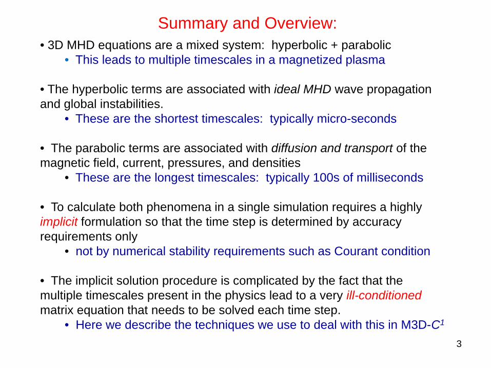
• 3D MHD equations are a mixed system: hyperbolic + parabolic• This leads to multiple timescales in a magnetized plasma
• The hyperbolic terms are associated with ideal MHD wave propagation and global instabilities.
• These are the shortest timescales: typically micro-seconds
• The parabolic terms are associated with diffusion and transport of the magnetic field, current, pressures, and densities
• These are the longest timescales: typically 100s of milliseconds
• To calculate both phenomena in a single simulation requires a highly implicit formulation so that the time step is determined by accuracy requirements only
• not by numerical stability requirements such as Courant condition
• The implicit solution procedure is complicated by the fact that the multiple timescales present in the physics lead to a very ill-conditionedmatrix equation that needs to be solved each time step.
• Here we describe the techniques we use to deal with this in M3D-C1
Summary and Overview:
4
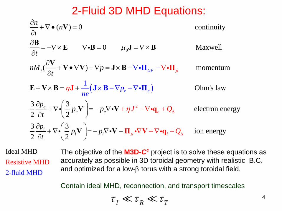
2-Fluid 3D MHD Equations:
( )
0
2
1
( ) 0 continuity
0 Maxwell
( ) momentum
Ohm's law
3 3 electron energy2 23 32 2
i
ee e
V
e e
e
ii
G
pn
n nt
t
nM pt
p p pt
J
t
e
p p
Q
μ
η
η
μ
Δ
∂+ ∇ • =
∂∂
= −∇× ∇ = = ∇ ×∂
∂+ • ∇ + ∇ = × −
∂
+ × = +
∂ ⎛ ⎞+ ∇ = − ∇⎜ ⎟∂ ⎝ ⎠∂ ⎛ ⎞+ ∇ ⎜ ⎟∂ ⎝ ⎠
∇ −
× − ∇ − ∇
∇
+ − ∇ +
V
B E B
Π
J
q
J B
V V V J B
E V B
V V
V
Π
J B Π
i
i
i
i
i
i
i i
ion energyi i Qp μ Δ∇ − ∇ −= − ∇ −Π qV Vi ii
Resistive MH2-
Idea
fluiD
d
l MHD
MHD
The objective of the M3D-C1 project is to solve these equations as accurately as possible in 3D toroidal geometry with realistic B.C. and optimized for a low-β torus with a strong toroidal field.
Contain ideal MHD, reconnection, and transport timescales
I R Tτ τ τ
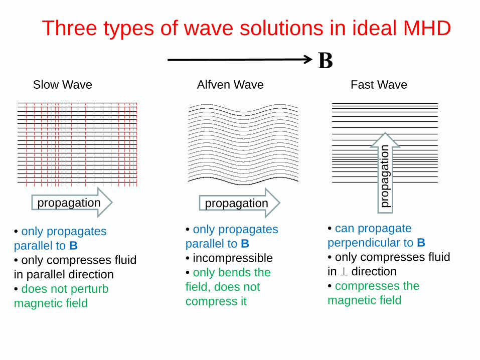
Slow Wave Alfven Wave Fast Wave
Three types of wave solutions in ideal MHD
propagation propagation prop
agat
ion
• only propagates parallel to B• only compresses fluid in parallel direction• does not perturb magnetic field
• only propagates parallel to B• incompressible• only bends the field, does not compress it
• can propagate perpendicular to B• only compresses fluid in ⊥ direction• compresses the magnetic field
B
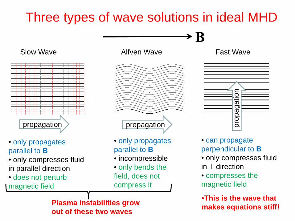
Plasma instabilities grow out of these two waves
•This is the wave that makes equations stiff!
B
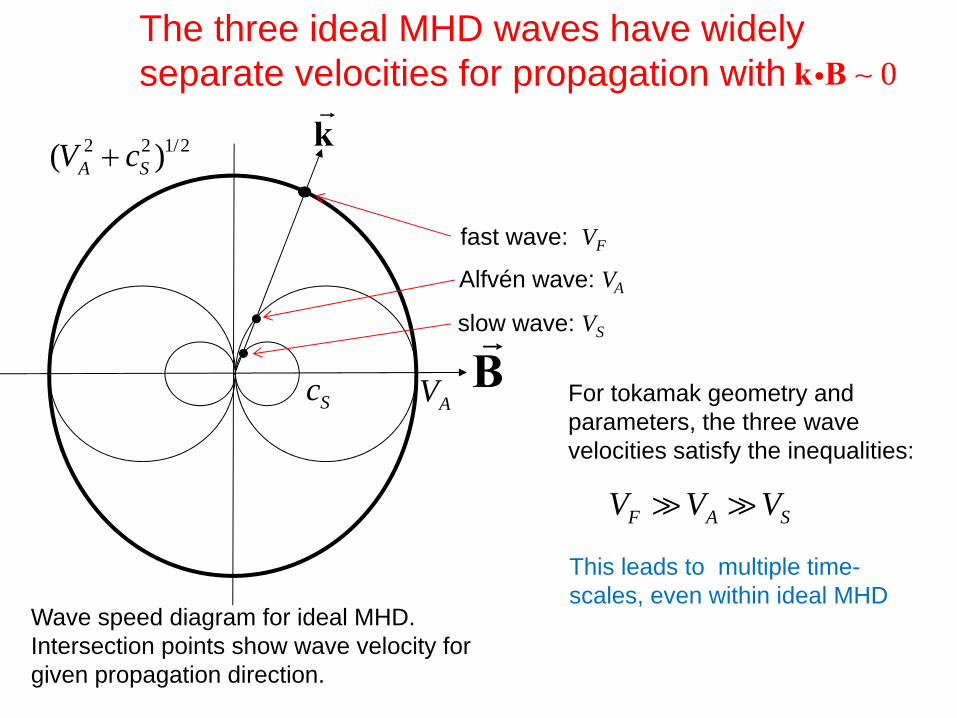
k2 2 1/2( )A SV c+
Sc AV
Wave speed diagram for ideal MHD. Intersection points show wave velocity for given propagation direction.
fast wave: VF
Alfvén wave: VA
slow wave: VS
The three ideal MHD waves have widely separate velocities for propagation with 0k Bi ∼
F A SV V V
For tokamak geometry and parameters, the three wave velocities satisfy the inequalities:
This leads to multiple time-scales, even within ideal MHD
8
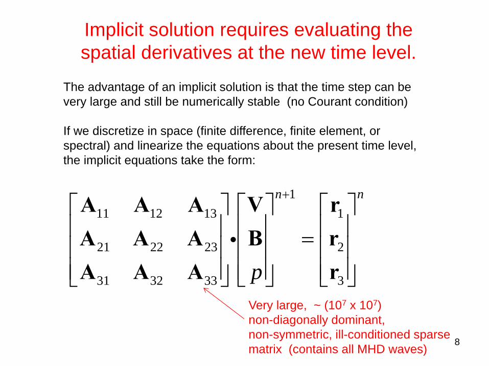
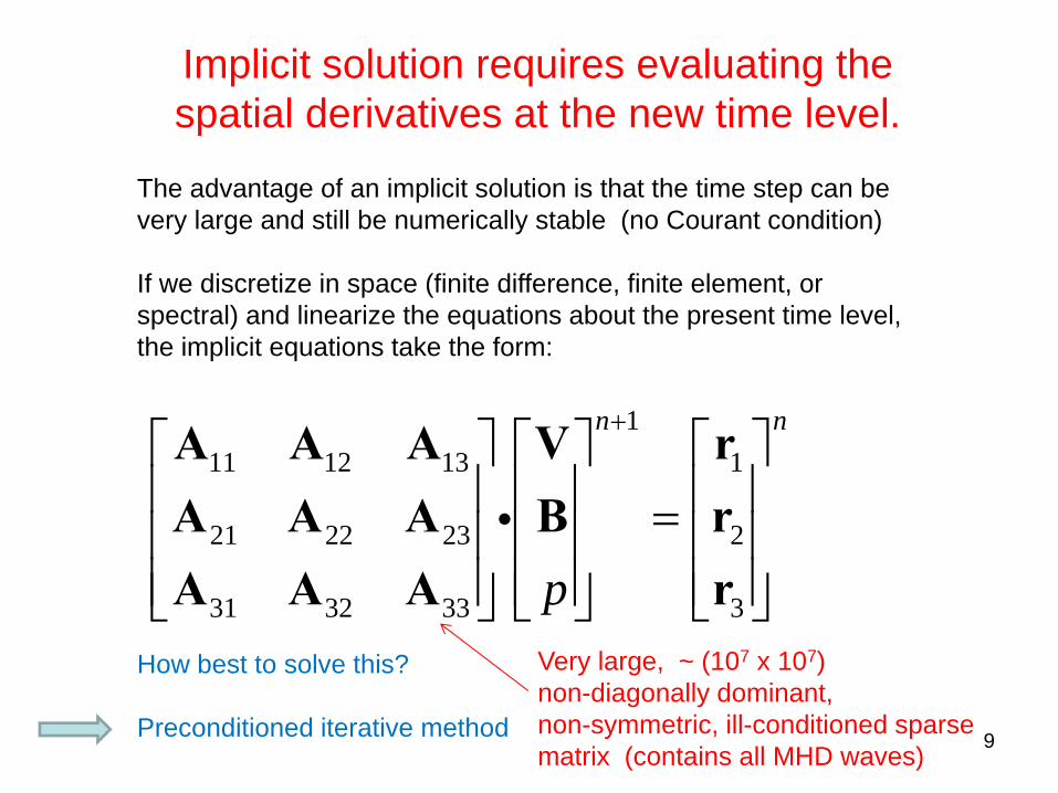
The advantage of an implicit solution is that the time step can be very large and still be numerically stable (no Courant condition)
If we discretize in space (finite difference, finite element, or spectral) and linearize the equations about the present time level, the implicit equations take the form:
111 12 13 1
21 22 23 2
31 32 33 3
n n
p
+⎡ ⎤ ⎡ ⎤ ⎡ ⎤⎢ ⎥ ⎢ ⎥ ⎢ ⎥=⎢ ⎥ ⎢ ⎥ ⎢ ⎥⎢ ⎥ ⎢ ⎥ ⎢ ⎥⎣ ⎦ ⎣ ⎦ ⎣ ⎦
A A A V rA A A B rA A A r
i
Implicit solution requires evaluating the spatial derivatives at the new time level.
Very large, ~ (107 x 107) non-diagonally dominant, non-symmetric, ill-conditioned sparse matrix (contains all MHD waves)
9
The advantage of an implicit solution is that the time step can be very large and still be numerically stable (no Courant condition)
If we discretize in space (finite difference, finite element, or spectral) and linearize the equations about the present time level, the implicit equations take the form:
How best to solve this?
Preconditioned iterative method
111 12 13 1
21 22 23 2
31 32 33 3
n n
p
+⎡ ⎤ ⎡ ⎤ ⎡ ⎤⎢ ⎥ ⎢ ⎥ ⎢ ⎥=⎢ ⎥ ⎢ ⎥ ⎢ ⎥⎢ ⎥ ⎢ ⎥ ⎢ ⎥⎣ ⎦ ⎣ ⎦ ⎣ ⎦
A A A V rA A A B rA A A r
i
Implicit solution requires evaluating the spatial derivatives at the new time level.
Very large, ~ (107 x 107) non-diagonally dominant, non-symmetric, ill-conditioned sparse matrix (contains all MHD waves)
10
Preconditioning
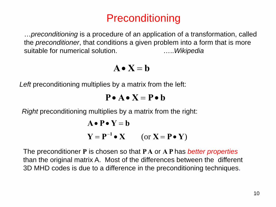
bXA =•
Left preconditioning multiplies by a matrix from the left:
bPXAP •=••Right preconditioning multiplies by a matrix from the right:
)or ( YP XXPYbYPA
1 •=•=
=••−
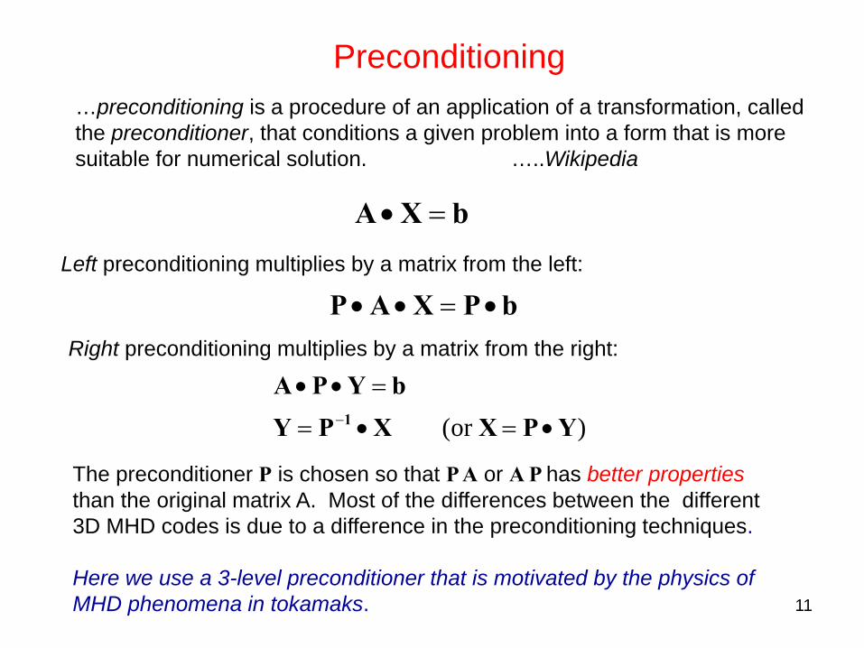
…preconditioning is a procedure of an application of a transformation, called the preconditioner, that conditions a given problem into a form that is more suitable for numerical solution. …..Wikipedia
The preconditioner P is chosen so that P A or A P has better properties than the original matrix A. Most of the differences between the different 3D MHD codes is due to a difference in the preconditioning techniques.
11
Preconditioning
bXA =•
Left preconditioning multiplies by a matrix from the left:
bPXAP •=••Right preconditioning multiplies by a matrix from the right:
)or ( YP XXPYbYPA
1 •=•=
=••−
…preconditioning is a procedure of an application of a transformation, called the preconditioner, that conditions a given problem into a form that is more suitable for numerical solution. …..Wikipedia
The preconditioner P is chosen so that P A or A P has better properties than the original matrix A. Most of the differences between the different 3D MHD codes is due to a difference in the preconditioning techniques.
Here we use a 3-level preconditioner that is motivated by the physics of MHD phenomena in tokamaks.
“In ending this book with the subject of preconditioners, we find ourselves at the philosophical center of the scientific computing of the future…
Nothing will be more central to computational science in the next century than the art of transforming a problem that appears intractable into another whose solution can be approximated rapidly.
For Krylov subspace matrix iterations, this is preconditioning.”
From:L. N. Trefethen and D. Bau, III, Numerical Linear Algebra (SIAM) 1997
More on Preconditioning
“ Direct solvers are often the best option for 2‐dimensional problems, but not for 3‐dimensional problems.
Generally speaking, preconditioning attempts to improve the spectral properties of the coefficient matrix. For symmetric positive definite problems, the rate of convergence of the CG method depends on the spectral radius.
For non‐symmetric problems, the situation is more complicated and the eigenvalues may not describe the convergence properties. Nevertheless, a clustered spectrum (away from 0) often results in rapid convergence, particularly when the preconditioned matrix is close to normal. “
FROM: Michele Benzi, “Preconditioning Techniques for Large Linear Systems: A Survey”, J. Comput. Phys. 182, 418‐477 (2002)
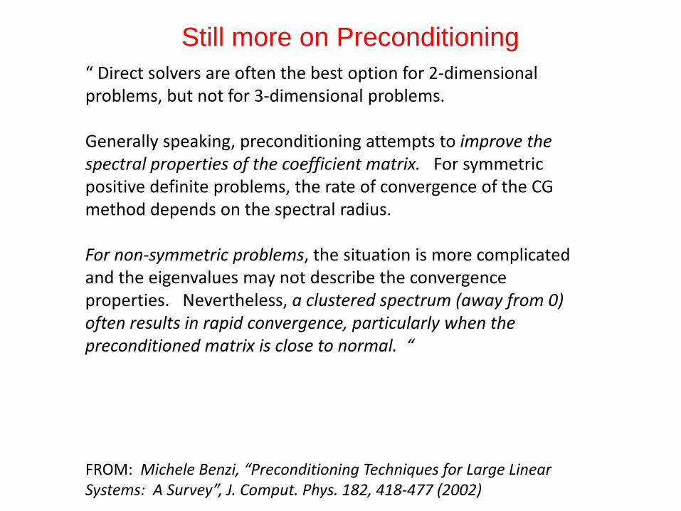
Still more on Preconditioning
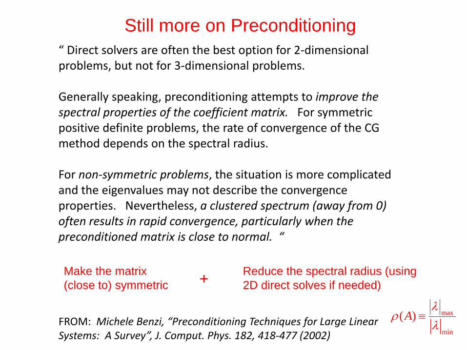
“ Direct solvers are often the best option for 2‐dimensional problems, but not for 3‐dimensional problems.
Generally speaking, preconditioning attempts to improve the spectral properties of the coefficient matrix. For symmetric positive definite problems, the rate of convergence of the CG method depends on the spectral radius.
For non‐symmetric problems, the situation is more complicated and the eigenvalues may not describe the convergence properties. Nevertheless, a clustered spectrum (away from 0) often results in rapid convergence, particularly when the preconditioned matrix is close to normal. “
FROM: Michele Benzi, “Preconditioning Techniques for Large Linear Systems: A Survey”, J. Comput. Phys. 182, 418‐477 (2002)
Still more on Preconditioning
Make the matrix (close to) symmetric
Reduce the spectral radius (using 2D direct solves if needed)+
max
min
( )Aλ
ρλ
≡
15
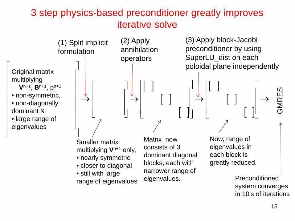
[ ][ ]
[ ]
[ ][ ]
[ ]
⎡ ⎤⎢ ⎥⎢ ⎥ ⎡ ⎤ ⎡ ⎤⎡ ⎤⎢ ⎥ ⎢ ⎥ ⎢ ⎥⎢ ⎥→ → → →⎢ ⎥ ⎢ ⎥ ⎢ ⎥⎢ ⎥⎢ ⎥ ⎢ ⎥ ⎢ ⎥⎢ ⎥⎣ ⎦ ⎣ ⎦ ⎣ ⎦⎢ ⎥⎢ ⎥⎣ ⎦
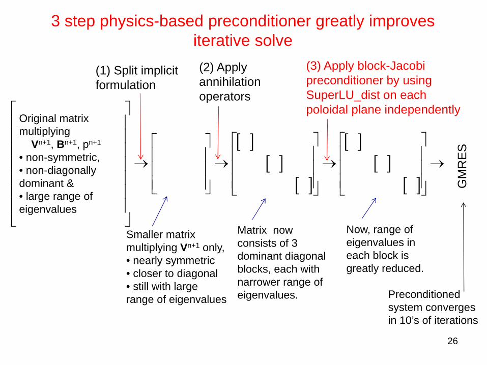
Original matrix multiplying
Vn+1, Bn+1, pn+1
• non-symmetric,• non-diagonally dominant & • large range of eigenvalues
(1) Split implicit formulation
Smaller matrix multiplying Vn+1 only, • nearly symmetric • closer to diagonal• still with large range of eigenvalues
(2) Apply annihilation operators
Matrix now consists of 3 dominant diagonal blocks, each with narrower range of eigenvalues.
(3) Apply block-Jacobi preconditioner by using SuperLU_dist on each poloidal plane independently
Now, range of eigenvalues in each block is greatly reduced.
GM
RE
S
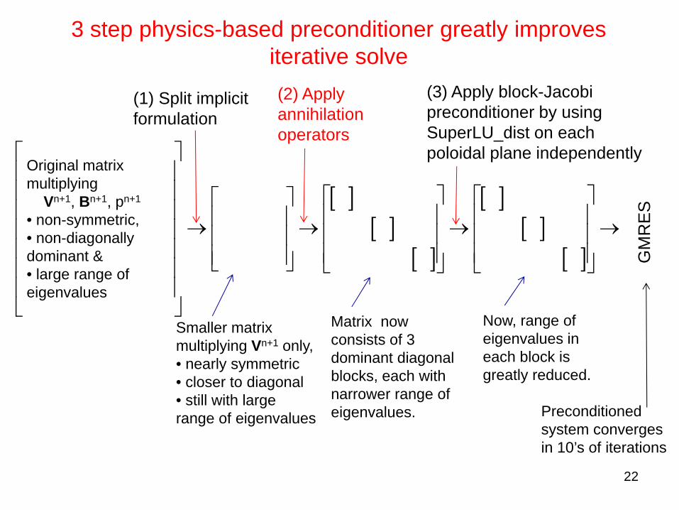
3 step physics-based preconditioner greatly improves iterative solve
Preconditioned system converges in 10’s of iterations
16
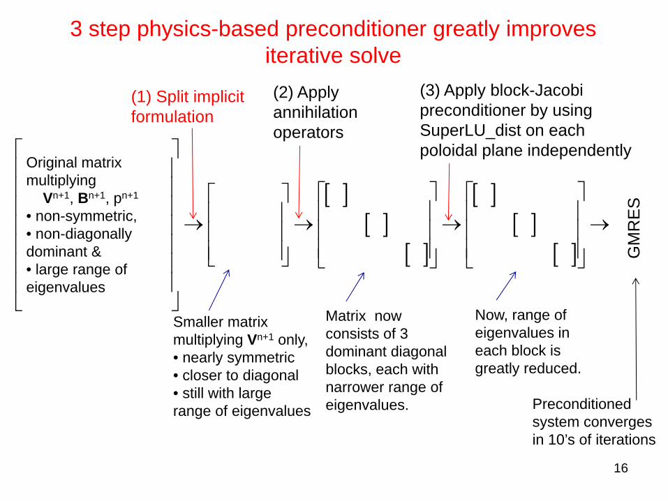
[ ][ ]
[ ]
[ ][ ]
[ ]
⎡ ⎤⎢ ⎥⎢ ⎥ ⎡ ⎤ ⎡ ⎤⎡ ⎤⎢ ⎥ ⎢ ⎥ ⎢ ⎥⎢ ⎥→ → → →⎢ ⎥ ⎢ ⎥ ⎢ ⎥⎢ ⎥⎢ ⎥ ⎢ ⎥ ⎢ ⎥⎢ ⎥⎣ ⎦ ⎣ ⎦ ⎣ ⎦⎢ ⎥⎢ ⎥⎣ ⎦
Original matrix multiplying
Vn+1, Bn+1, pn+1
• non-symmetric,• non-diagonally dominant & • large range of eigenvalues
(1) Split implicit formulation
Smaller matrix multiplying Vn+1 only, • nearly symmetric • closer to diagonal• still with large range of eigenvalues
(2) Apply annihilation operators
Matrix now consists of 3 dominant diagonal blocks, each with narrower range of eigenvalues.
(3) Apply block-Jacobi preconditioner by using SuperLU_dist on each poloidal plane independently
Now, range of eigenvalues in each block is greatly reduced.
GM
RE
S
3 step physics-based preconditioner greatly improves iterative solve
Preconditioned system converges in 10’s of iterations
17
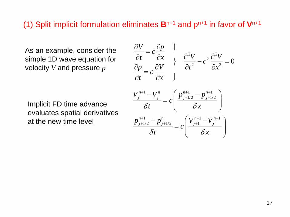
(1) Split implicit formulation eliminates Bn+1 and pn+1 in favor of Vn+1
2 22
2 2 0
V pcV Vt x c
p V t xct x
∂ ∂ ⎫= ⎪ ∂ ∂⎪∂ ∂ − =⎬∂ ∂ ∂ ∂⎪=⎪∂ ∂ ⎭
1 1 11/2 1/2
1 1 11/2 1/2 1
n n n nj j j j
n n n nj j j j
V V p pc
t x
p p V Vc
t x
δ δ
δ δ
+ + ++ −
+ + ++ + +
⎛ ⎞− −= ⎜ ⎟⎜ ⎟
⎝ ⎠⎛ ⎞− −
= ⎜ ⎟⎜ ⎟⎝ ⎠
As an example, consider the simple 1D wave equation for velocity V and pressure p
Implicit FD time advance evaluates spatial derivatives at the new time level
18
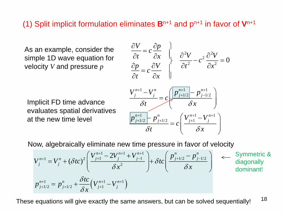
(1) Split implicit formulation eliminates Bn+1 and pn+1 in favor of Vn+1
2 22
2 2 0
V pcV Vt x c
p V t xct x
∂ ∂ ⎫= ⎪ ∂ ∂⎪∂ ∂ − =⎬∂ ∂ ∂ ∂⎪=⎪∂ ∂ ⎭
( )
1 1 11 1 1/2 1/21 2
2
1 1 11/2 1/2 1
2( )
n n n n nj j j j jn n
j j
n n n nj j j j
V V V p pV V tc tc
x x
tcp p V Vx
δ δδ δ
δδ
+ + ++ − + −+
+ + ++ + +
⎛ ⎞ ⎛ ⎞− + −= + +⎜ ⎟ ⎜ ⎟⎜ ⎟ ⎜ ⎟
⎝ ⎠ ⎝ ⎠
= + −
As an example, consider the simple 1D wave equation for velocity V and pressure p
Implicit FD time advance evaluates spatial derivatives at the new time level
1 1 11/2 1/2
1 1 11/2 1/2 1
n n n nj j j j
n n n nj j j j
V V p pc
t x
p p V Vc
t x
δ δ
δ δ
+ + ++ −
+ + ++ + +
⎛ ⎞− −= ⎜ ⎟⎜ ⎟
⎝ ⎠⎛ ⎞− −
= ⎜ ⎟⎜ ⎟⎝ ⎠
Now, algebraically eliminate new time pressure in favor of velocity
These equations will give exactly the same answers, but can be solved sequentially!
Symmetric & diagonally dominant!
19
2 2
2 2 2
2 2 2
2 2 2
2 2 2
2 2
1 211 21
1 211 21
1 211 21
1 11 1
1 11 1
1 11 1
S SSS S SS S
S S SS SS S SS S
S S SS SS SS S
S SS S
S SS S
S SS
⎡ ⎤+ −−⎡ ⎤⎢ ⎥⎢ ⎥ − + −− ⎢ ⎥⎢ ⎥⎢ ⎥⎢ ⎥ − + −−⎢ ⎥⎢ ⎥ − + −− ⎢ ⎥⎢ ⎥⎢ ⎥⎢ ⎥ − + −−⎢ ⎥⎢ ⎥
− +− ⎢ ⎥⎣ ⎦⎢ ⎥⎢ ⎥− ⎡ ⎤⎢ ⎥ ⎢ ⎥−⎢ ⎥ ⎢ ⎥⎢ ⎥− ⎢ ⎥⎢ ⎥ ⎢ ⎥⎢ ⎥− ⎢ ⎥⎢ ⎥ ⎢ ⎥−⎢ ⎥ ⎢ ⎥⎢ ⎥⎣ ⎦ ⎣ ⎦
2N
N
N
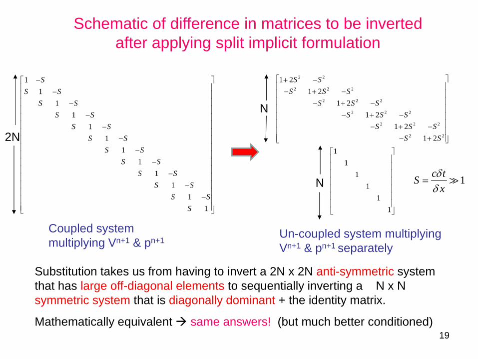
Substitution takes us from having to invert a 2N x 2N anti-symmetric system that has large off-diagonal elements to sequentially inverting a N x N symmetric system that is diagonally dominant + the identity matrix.
Mathematically equivalent same answers! (but much better conditioned)
Schematic of difference in matrices to be inverted after applying split implicit formulation
1c tSx
δδ
=
Coupled system multiplying Vn+1 & pn+1
Un-coupled system multiplying Vn+1 & pn+1 separately
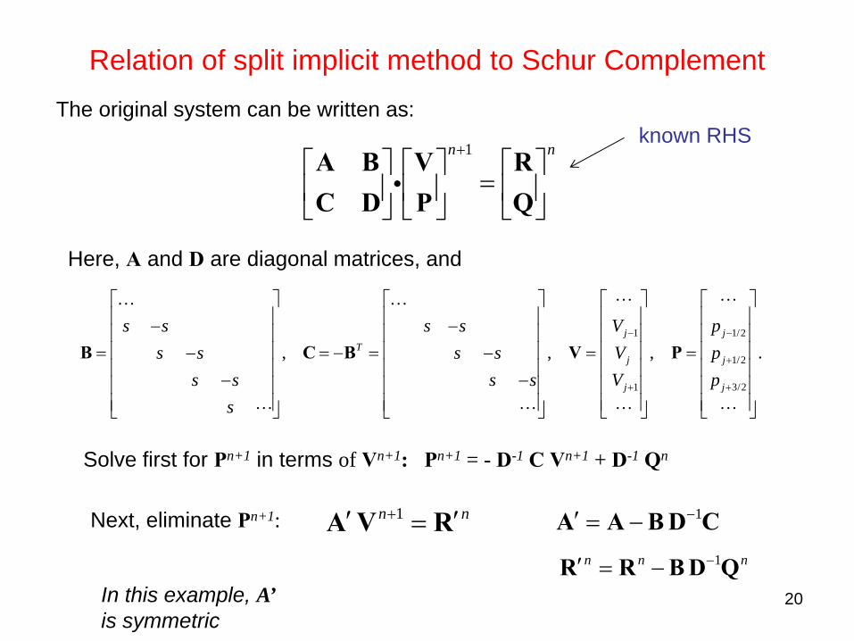
Relation of split implicit method to Schur Complement
20
1n n+⎡ ⎤ ⎡ ⎤ ⎡ ⎤
=⎢ ⎥ ⎢ ⎥ ⎢ ⎥⎣ ⎦ ⎣ ⎦ ⎣ ⎦
A B V RC D P Q
i
1 1/2
1/2
1 3/2
, , , .j j
Tj j
j j
s s s s V ps s s s V p
s s s s V ps
− −
+
+ +
⎡ ⎤ ⎡ ⎤ ⎡ ⎤ ⎡ ⎤⎢ ⎥ ⎢ ⎥ ⎢ ⎥ ⎢ ⎥− −⎢ ⎥ ⎢ ⎥ ⎢ ⎥ ⎢ ⎥⎢ ⎥ ⎢ ⎥ ⎢ ⎥ ⎢ ⎥= = − = = =− −⎢ ⎥ ⎢ ⎥ ⎢ ⎥ ⎢ ⎥− −⎢ ⎥ ⎢ ⎥ ⎢ ⎥ ⎢ ⎥⎢ ⎥ ⎢ ⎥ ⎢ ⎥ ⎢ ⎥⎣ ⎦ ⎣ ⎦ ⎣ ⎦ ⎣ ⎦
B C B V P
… …
1n n+′ ′=A V R 1−′ = −A A B D C1n n n−′ = −R R B D Q
The original system can be written as:
Here, A and D are diagonal matrices, and
Solve first for Pn+1 in terms of Vn+1: Pn+1 = - D-1 C Vn+1 + D-1 Qn
Next, eliminate Pn+1:
known RHS
In this example, A’is symmetric
21
[ ]
[ ]
00
1 p
p p p
ρμ
γ
= ∇× × − ∇
= ∇× ×
= − ∇ − ∇
V B B
B V BV Vi i
( ) ( ) ( )
( )( ) ( )
00
1 t t p tp
t
p t p p t
ρ θδ θδ θδμ
θδ
θδ γ θδ
⎡ ⎤= ∇× + × + − ∇ +⎣ ⎦
⎡ ⎤= ∇× + ×⎣ ⎦
= − + ∇ − ∇ +
V B B B B
B V V B
V V V Vi i
{ } { }2 2 1 2 2
0
1( ) ( ) ( )n
n nt L t L t pρ θ δ ρ θ δ δμ
+ ⎧ ⎫− = − + −∇ + ∇× ×⎨ ⎬
⎩ ⎭V V B B
{ } ( ){ } ( ) ( )( )
0 0
1 1L
p pμ μ
γ
= ∇× ∇× × × + ∇× × ∇× ×⎡ ⎤ ⎡ ⎤⎣ ⎦ ⎣ ⎦
+∇ ∇ + ∇
V V B B B V B
V Vi i
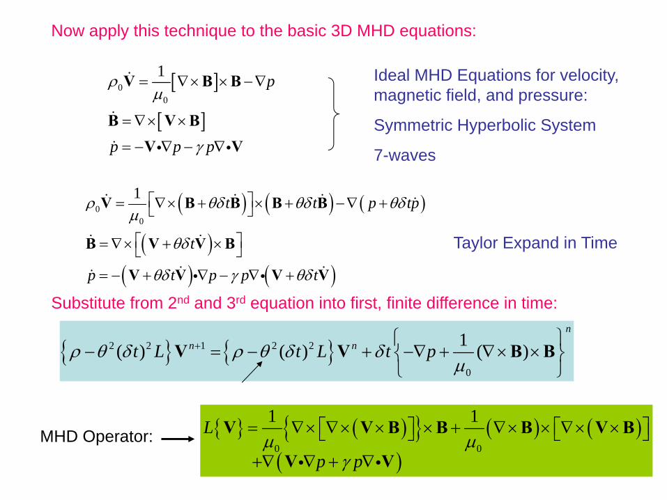
Now apply this technique to the basic 3D MHD equations:
Ideal MHD Equations for velocity, magnetic field, and pressure:
Symmetric Hyperbolic System
7-waves
Taylor Expand in Time
Substitute from 2nd and 3rd equation into first, finite difference in time:
MHD Operator:
22
[ ][ ]
[ ]
[ ][ ]
[ ]
⎡ ⎤⎢ ⎥⎢ ⎥ ⎡ ⎤ ⎡ ⎤⎡ ⎤⎢ ⎥ ⎢ ⎥ ⎢ ⎥⎢ ⎥→ → → →⎢ ⎥ ⎢ ⎥ ⎢ ⎥⎢ ⎥⎢ ⎥ ⎢ ⎥ ⎢ ⎥⎢ ⎥⎣ ⎦ ⎣ ⎦ ⎣ ⎦⎢ ⎥⎢ ⎥⎣ ⎦
Original matrix multiplying
Vn+1, Bn+1, pn+1
• non-symmetric,• non-diagonally dominant & • large range of eigenvalues
(1) Split implicit formulation
Smaller matrix multiplying Vn+1 only, • nearly symmetric • closer to diagonal• still with large range of eigenvalues
(2) Apply annihilation operators
Matrix now consists of 3 dominant diagonal blocks, each with narrower range of eigenvalues.
(3) Apply block-Jacobi preconditioner by using SuperLU_dist on each poloidal plane independently
Now, range of eigenvalues in each block is greatly reduced.
GM
RE
S
3 step physics-based preconditioner greatly improves iterative solve
Preconditioned system converges in 10’s of iterations
23
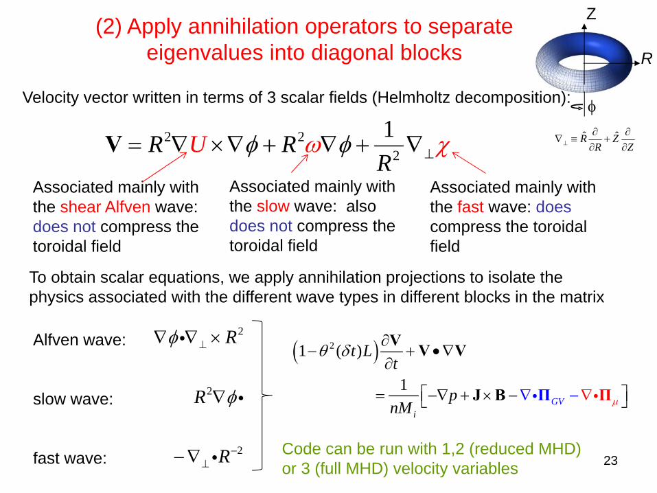
(2) Apply annihilation operators to separate eigenvalues into diagonal blocks
2 22
1RR
UR ωφ φ χ⊥= ∇ ×∇ + ∇ + ∇V
φ
Z
R
Associated mainly with the shear Alfven wave: does not compress the toroidal field
Associated mainly with the slow wave: also does not compress the toroidal field
Associated mainly with the fast wave: doescompress the toroidal field
To obtain scalar equations, we apply annihilation projections to isolate the physics associated with the different wave types in different blocks in the matrix
2
2
2
R
R
R
φ
φ
⊥
−⊥
∇ ∇ ×
∇
− ∇
i
i
i
( )21 ( )
1
iGV
t Lt
pnM μ
θ δ ∂− + • ∇
∂
⎡ ⎤= −∇ + × ∇−⎣ ⎦∇ −
V V
J Π
V
B Π ii
Alfven wave:
slow wave:
fast wave:
Velocity vector written in terms of 3 scalar fields (Helmholtz decomposition):
Code can be run with 1,2 (reduced MHD) or 3 (full MHD) velocity variables
ˆ ˆR ZR Z⊥
∂ ∂∇ ≡ +
∂ ∂
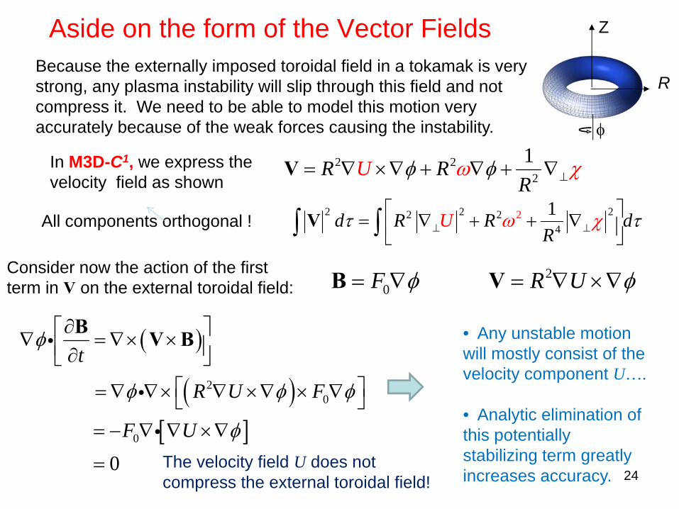
Aside on the form of the Vector Fields
24
Because the externally imposed toroidal field in a tokamak is very strong, any plasma instability will slip through this field and not compress it. We need to be able to model this motion very accurately because of the weak forces causing the instability.
2 22
1RR
UR ωφ φ χ⊥= ∇ ×∇ + ∇ + ∇V
( )
( )[ ]
20
0
0
t
R U F
F U
φ
φ φ φ
φ
∂⎡ ⎤∇ = ∇× ×⎢ ⎥∂⎣ ⎦⎡ ⎤= ∇ ∇× ∇ ×∇ × ∇⎣ ⎦
= − ∇ ∇ ×∇
=
B V Bi
i
i
In M3D-C1, we express the velocity field as shown
Consider now the action of the first term in V on the external toroidal field:
• Any unstable motion will mostly consist of the velocity component U….
• Analytic elimination of this potentially stabilizing term greatly increases accuracy.
The velocity field U does not compress the external toroidal field!
20F R Uφ φ= ∇ = ∇ ×∇B V
φ
Z
R
All components orthogonal !2 2
422 22 1Ud R R d
Rτ τω χ⊥ ⊥
⎡ ⎤= ∇ + + ∇⎢ ⎥⎣ ⎦∫ ∫V
8/4/2011
25
1 2 310-6
10-5
10-4
10-3
10-2
10-1
100
101
102
103
104
105
106
107
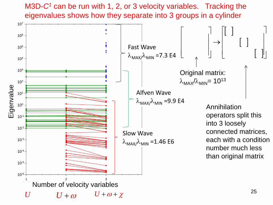
Fast WaveλMAX/λMIN =7.3 E4
Alfven WaveλMAX/λMIN =9.9 E4
Slow WaveλMAX/λMIN =1.46 E6
[ ][ ]
[ ]
⎡ ⎤⎡ ⎤⎢ ⎥⎢ ⎥ → ⎢ ⎥⎢ ⎥⎢ ⎥⎢ ⎥⎣ ⎦ ⎣ ⎦
Original matrix: λMAX/λMIN= 1013
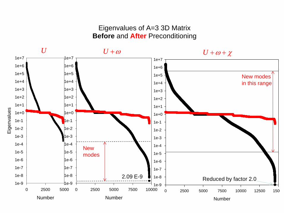
M3D-C1 can be run with 1, 2, or 3 velocity variables. Tracking the eigenvalues shows how they separate into 3 groups in a cylinder
U ω+ U ω χ+ +
Eig
enva
lue
UNumber of velocity variables
Annihilation operators split this into 3 loosely connected matrices, each with a condition number much less than original matrix
26
[ ][ ]
[ ]
[ ][ ]
[ ]
⎡ ⎤⎢ ⎥⎢ ⎥ ⎡ ⎤ ⎡ ⎤⎡ ⎤⎢ ⎥ ⎢ ⎥ ⎢ ⎥⎢ ⎥→ → → →⎢ ⎥ ⎢ ⎥ ⎢ ⎥⎢ ⎥⎢ ⎥ ⎢ ⎥ ⎢ ⎥⎢ ⎥⎣ ⎦ ⎣ ⎦ ⎣ ⎦⎢ ⎥⎢ ⎥⎣ ⎦
Original matrix multiplying
Vn+1, Bn+1, pn+1
• non-symmetric,• non-diagonally dominant & • large range of eigenvalues
(1) Split implicit formulation
Smaller matrix multiplying Vn+1 only, • nearly symmetric • closer to diagonal• still with large range of eigenvalues
(2) Apply annihilation operators
Matrix now consists of 3 dominant diagonal blocks, each with narrower range of eigenvalues.
(3) Apply block-Jacobi preconditioner by using SuperLU_dist on each poloidal plane independently
Now, range of eigenvalues in each block is greatly reduced.
GM
RE
S
3 step physics-based preconditioner greatly improves iterative solve
Preconditioned system converges in 10’s of iterations
27
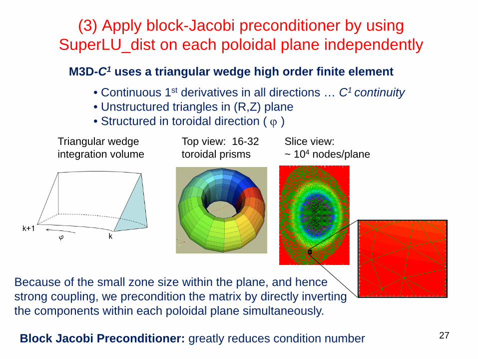
M3D-C1 uses a triangular wedge high order finite element
(3) Apply block-Jacobi preconditioner by using SuperLU_dist on each poloidal plane independently
Block Jacobi Preconditioner: greatly reduces condition number
Top view: 16-32 toroidal prisms
Slice view: ~ 104 nodes/plane
• Continuous 1st derivatives in all directions … C1 continuity• Unstructured triangles in (R,Z) plane• Structured in toroidal direction ( ϕ )
Triangular wedge integration volume
Because of the small zone size within the plane, and hence strong coupling, we precondition the matrix by directly inverting the components within each poloidal plane simultaneously.
28
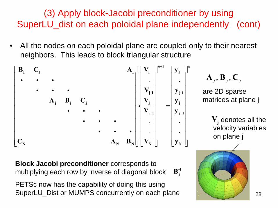
(3) Apply block-Jacobi preconditioner by using SuperLU_dist on each poloidal plane independently (cont)
• All the nodes on each poloidal plane are coupled only to their nearest neighbors. This leads to block triangular structure
11 1 1
.
.
.
n n+⎡ ⎤ ⎡ ⎤⎡ ⎤⎢ ⎥ ⎢ ⎥⎢ ⎥⎢ ⎥ ⎢ ⎥⎢ ⎥⎢ ⎥ ⎢ ⎥⎢ ⎥⎢ ⎥ ⎢ ⎥⎢ ⎥⎢ ⎥ ⎢ ⎥⎢ ⎥ =⎢ ⎥ ⎢ ⎥⎢ ⎥⎢ ⎥ ⎢ ⎥⎢ ⎥⎢ ⎥ ⎢ ⎥⎢ ⎥⎢ ⎥ ⎢ ⎥⎢ ⎥⎢ ⎥ ⎢ ⎥⎢ ⎥⎢ ⎥ ⎢ ⎥⎢ ⎥⎣ ⎦ ⎣ ⎦ ⎣ ⎦
1 1
j-1 j-1
j jj j j
j+1 j+1
N NN N N
V yB C A.
V yV yA B CV y
.
.V yC A B
i i ii i i
ii i i
i i ii i i
Block Jacobi preconditioner corresponds to multiplying each row by inverse of diagonal block
PETSc now has the capability of doing this using SuperLU_Dist or MUMPS concurrently on each plane
-1jB
, ,j j jA B C
are 2D sparse matrices at plane j
jV denotes all the velocity variables on plane j
29
NUMVAR=1
Number
0 2500 5000
Eige
nval
ues
1e-9
1e-8
1e-7
1e-6
1e-5
1e-4
1e-3
1e-2
1e-1
1e+0
1e+1
1e+2
1e+3
1e+4
1e+5
1e+6
1e+7NUMVAR=2
Number
0 2500 5000 7500 100001e-9
1e-8
1e-7
1e-6
1e-5
1e-4
1e-3
1e-2
1e-1
1e+0
1e+1
1e+2
1e+3
1e+4
1e+5
1e+6
1e+7NUMVAR=3
Number
0 2500 5000 7500 10000 12500 15001e-9
1e-8
1e-7
1e-6
1e-5
1e-4
1e-3
1e-2
1e-1
1e+0
1e+1
1e+2
1e+3
1e+4
1e+5
1e+6
1e+7
Eigenvalues of A=3 3D MatrixBefore and After Preconditioning
New modes in this range
New modes
2.09 E-9 Reduced by factor 2.0
U U ω+ U ω χ+ +
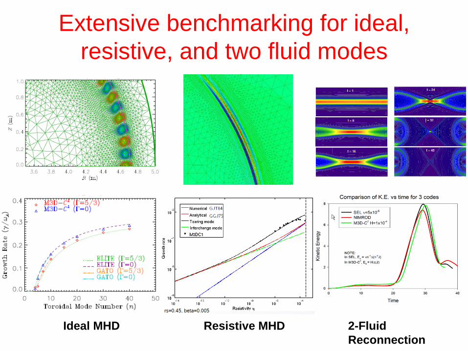
Extensive benchmarking for ideal, resistive, and two fluid modes
Ideal MHD Resistive MHD 2-Fluid Reconnection
31
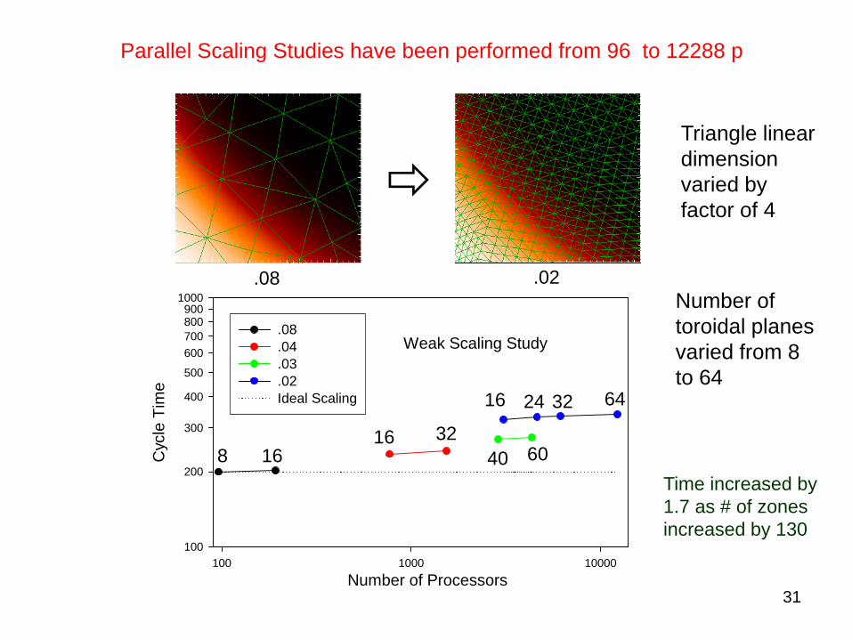
Weak Scaling Study
Number of Processors100 1000 10000
Cyc
le T
ime
100
200
300
400
500
600700800900
1000
.08
.04
.03
.02 Ideal Scaling
.08 .02
8 1616 32
40 60
16 24 32 64
Number of toroidal planes varied from 8 to 64
Parallel Scaling Studies have been performed from 96 to 12288 p
Triangle linear dimension varied by factor of 4
Time increased by 1.7 as # of zones increased by 130
32
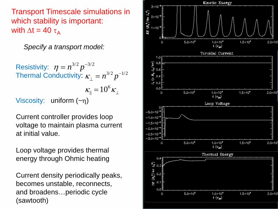
Resistivity:Thermal Conductivity:
Viscosity: uniform (~η)
Current controller provides loop voltage to maintain plasma current at initial value.
Loop voltage provides thermal energy through Ohmic heating
Current density periodically peaks, becomes unstable, reconnects, and broadens…periodic cycle (sawtooth)
Transport Timescale simulations in which stability is important: with Δt = 40 τA
3/2 1/2
610
n pκ
κ κ
−⊥
⊥
=
=
3/2 3/2n pη −=
Specify a transport model:
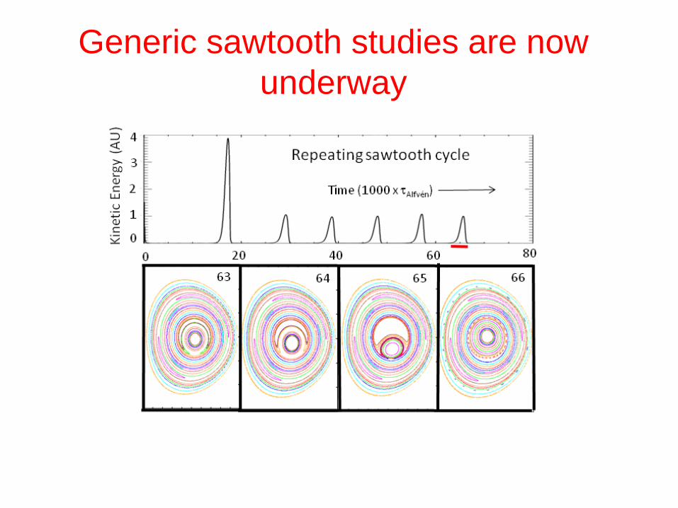
Generic sawtooth studies are now underway
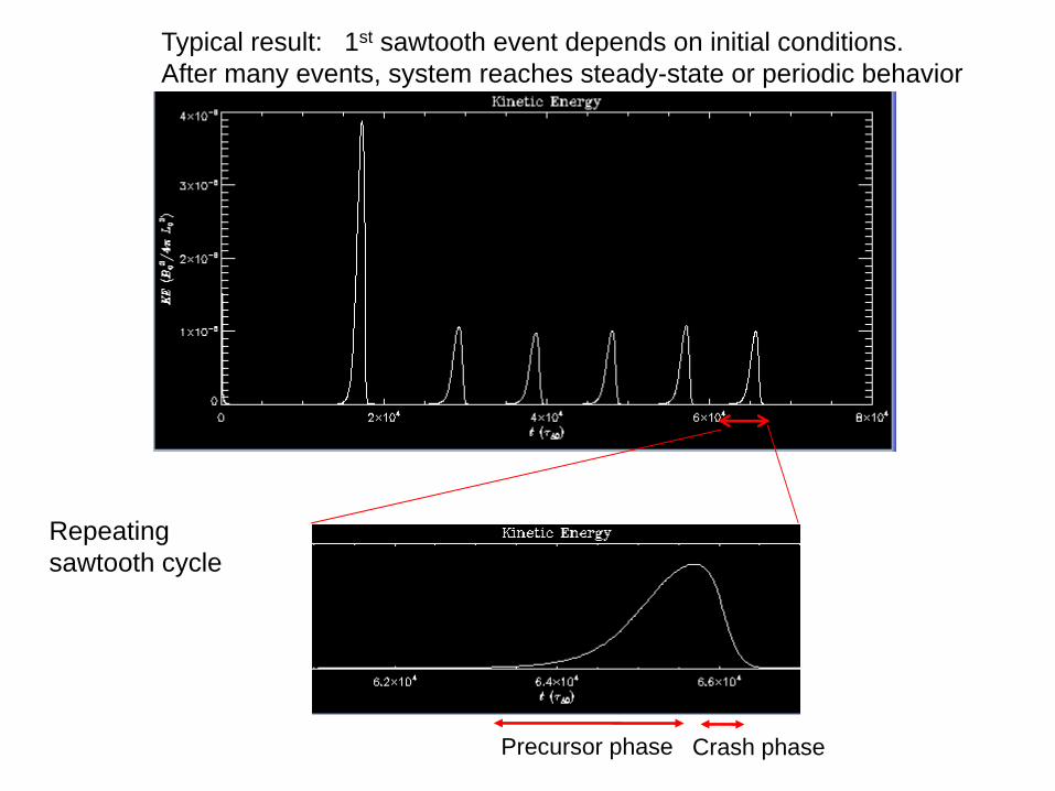
Typical result: 1st sawtooth event depends on initial conditions. After many events, system reaches steady-state or periodic behavior
Repeating sawtooth cycle
Precursor phase Crash phase
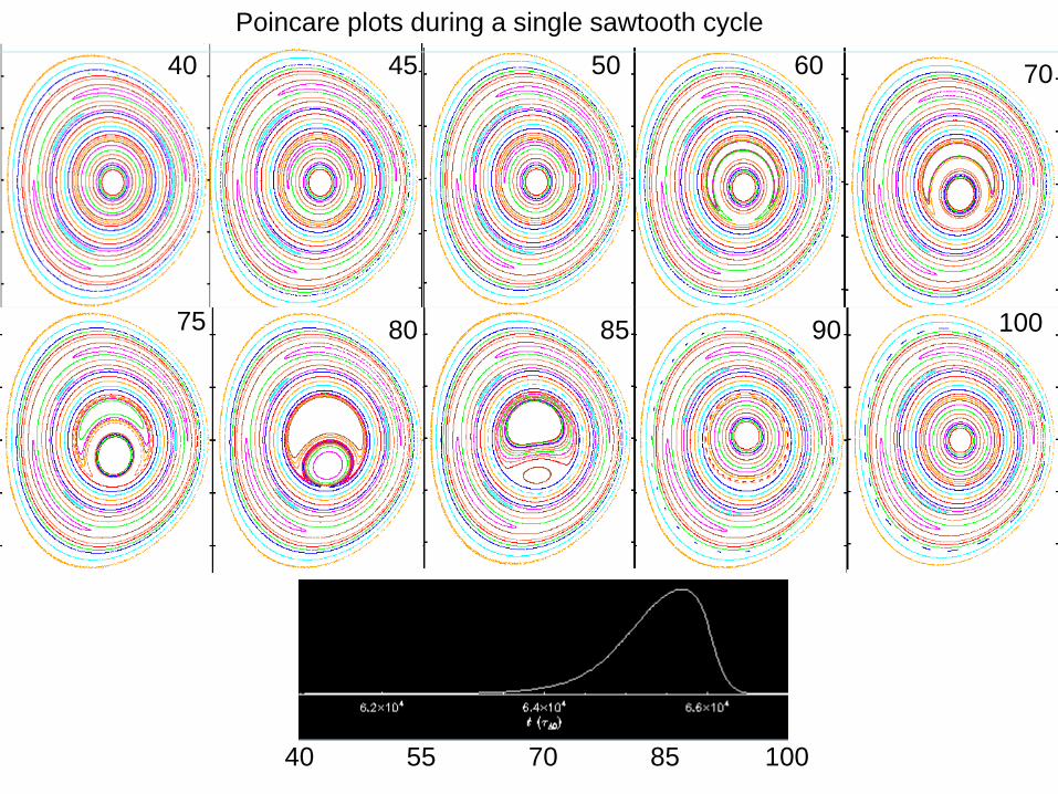
40 45 50 60 70
75 80 85 90 100
10040 7055 85
Poincare plots during a single sawtooth cycle
37
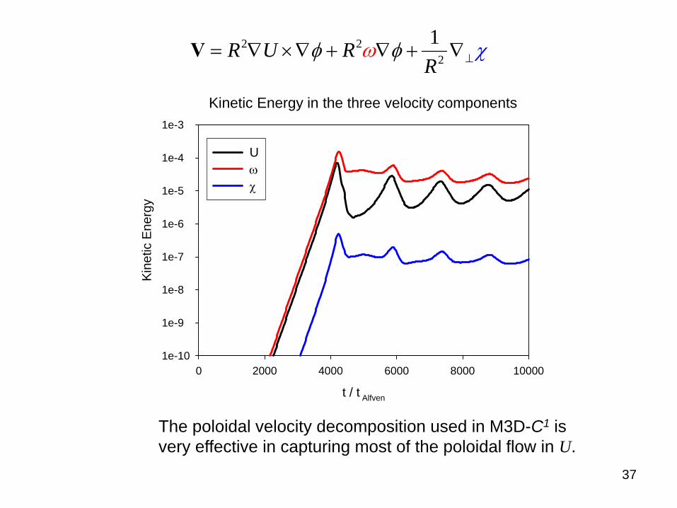
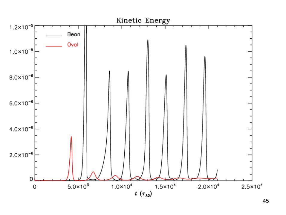
Kinetic Energy in the three velocity components
t / t Alfven
0 2000 4000 6000 8000 10000
Kine
tic E
nerg
y
1e-10
1e-9
1e-8
1e-7
1e-6
1e-5
1e-4
1e-3
Uωχ
2 22
1R U RR
ωφ φ χ⊥= ∇ ×∇ + ∇ + ∇V
The poloidal velocity decomposition used in M3D-C1 is very effective in capturing most of the poloidal flow in U.
38
Stationary States with Flow
In lower viscosity cases, the sawtooth behavior stops after a few cycles, and a central helical (1,1) structure forms with flow.
This flow is such as to flatten the central pressure and temperature. This flattening causes the current density to also flatten near the center, keeping q0 ~ 1 in the central region.
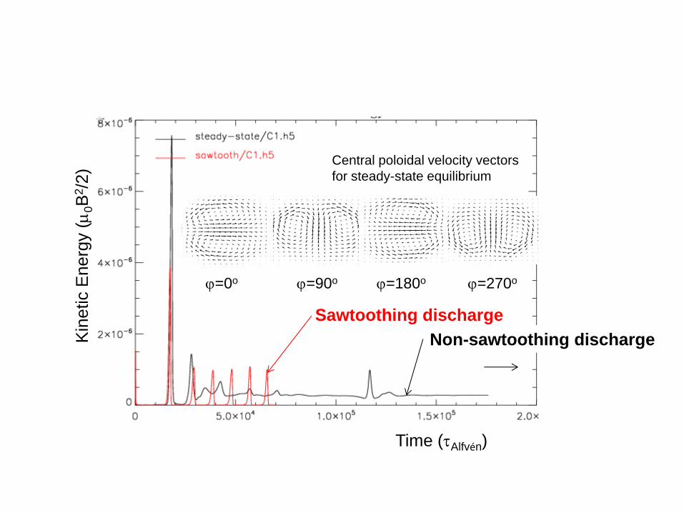
Sawtoothing dischargeNon-sawtoothing discharge
ϕ=0o ϕ=90o ϕ=180o ϕ=270o
Central poloidal velocity vectors for steady-state equilibrium
Kin
etic
Ene
rgy
(μ0B
2 /2)
Time (τAlfvén)
40
2D
minor radius
0.0 0.2 0.4 0.6 0.8 1.0
q-pr
ofile
0.5
1.0
1.5
2.0
2.5
3.0
3.5
4.0
4.5
t=0 t=24000 t=48000 t=96000
3D
minor radius
0.0 0.2 0.4 0.6 0.8 1.0
q-pr
ofile
0.5
1.0
1.5
2.0
2.5
3.0
3.5
4.0
4.5
t=0 t=24000 t=48000 t=96000
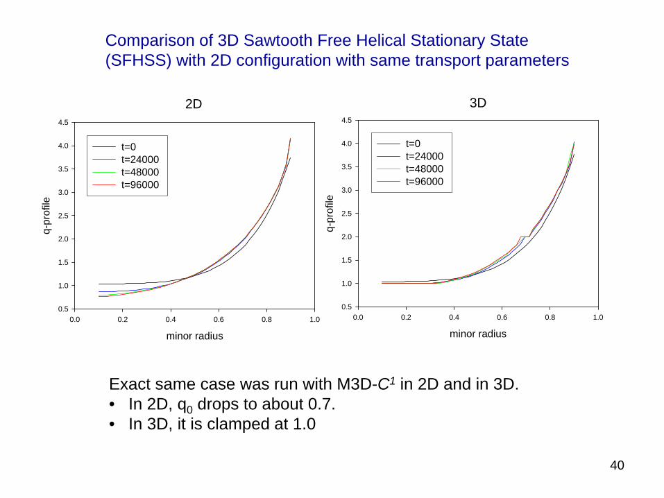
Exact same case was run with M3D-C1 in 2D and in 3D.• In 2D, q0 drops to about 0.7. • In 3D, it is clamped at 1.0
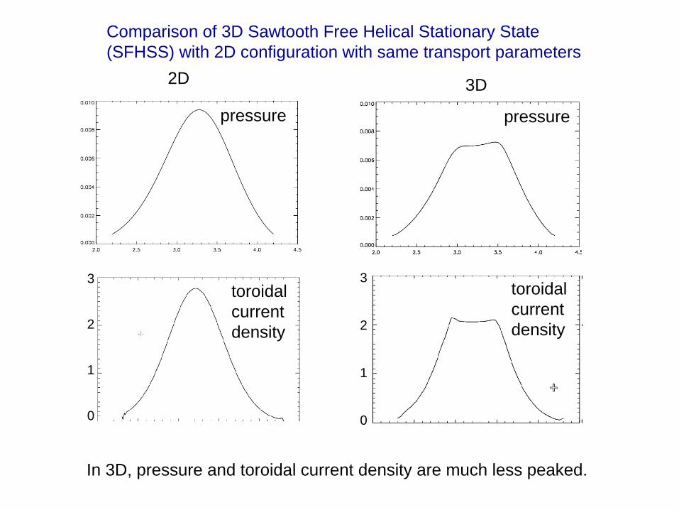
Comparison of 3D Sawtooth Free Helical Stationary State (SFHSS) with 2D configuration with same transport parameters
0
1
2
3
0
1
2
3
2D 3D
pressure pressure
toroidalcurrent density
toroidalcurrent density
In 3D, pressure and toroidal current density are much less peaked.
Comparison of 3D Sawtooth Free Helical Stationary State (SFHSS) with 2D configuration with same transport parameters
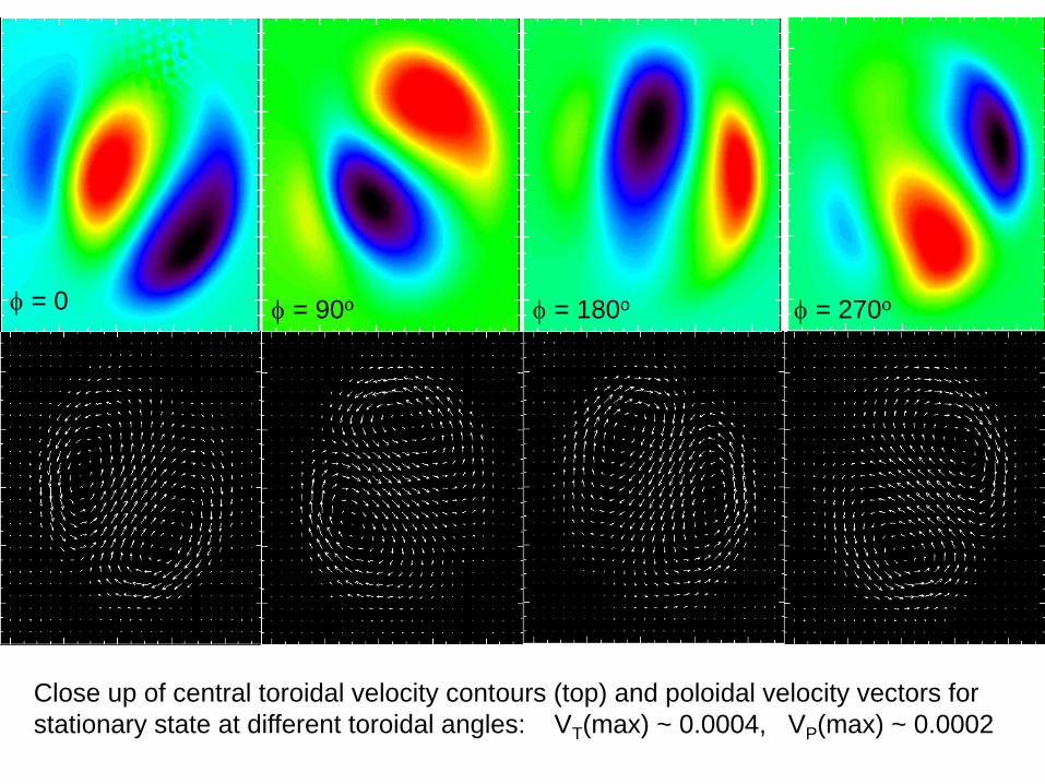
Close up of central toroidal velocity contours (top) and poloidal velocity vectors for stationary state at different toroidal angles: VT(max) ~ 0.0004, VP(max) ~ 0.0002
φ = 0 φ = 90o φ = 180o φ = 270o
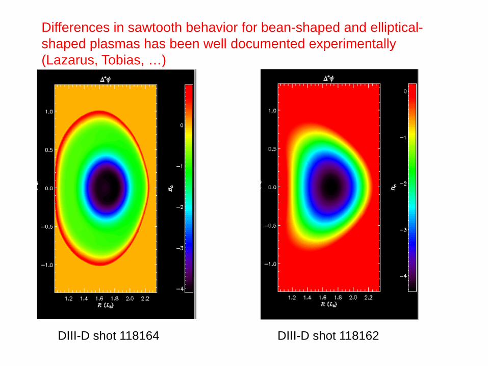
DIII-D shot 118164 DIII-D shot 118162
Differences in sawtooth behavior for bean-shaped and elliptical-shaped plasmas has been well documented experimentally (Lazarus, Tobias, …)
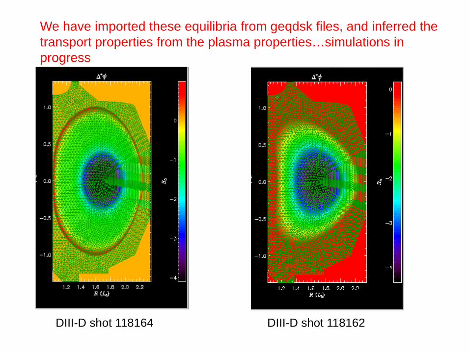
DIII-D shot 118164 DIII-D shot 118162
We have imported these equilibria from geqdsk files, and inferred the transport properties from the plasma properties…simulations in progress
45
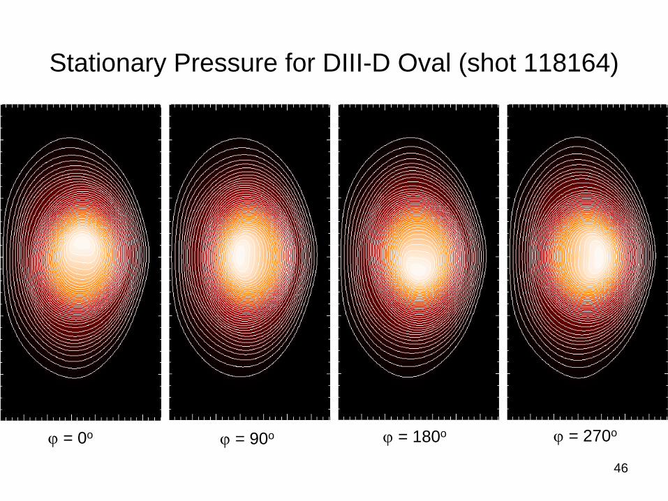
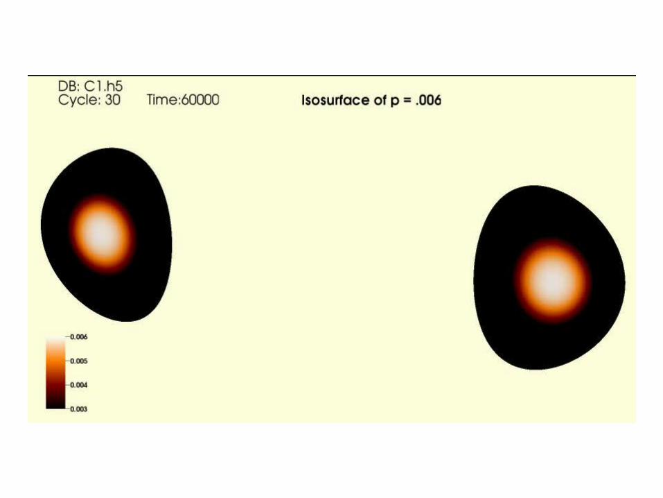
Stationary Pressure for DIII-D Oval (shot 118164)
46
ϕ = 0o ϕ = 90o ϕ = 180o ϕ = 270o
47
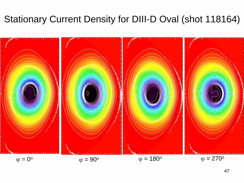
Stationary Current Density for DIII-D Oval (shot 118164)
ϕ = 0o ϕ = 90o ϕ = 180o ϕ = 270o
48
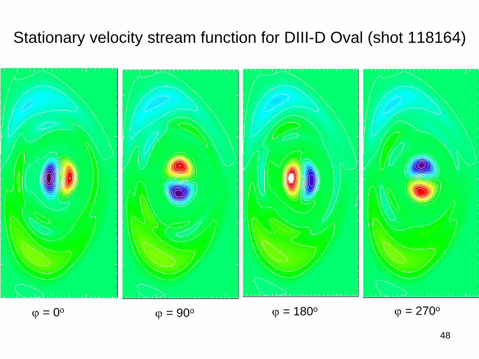
Stationary velocity stream function for DIII-D Oval (shot 118164)
ϕ = 0o ϕ = 90o ϕ = 180o ϕ = 270o
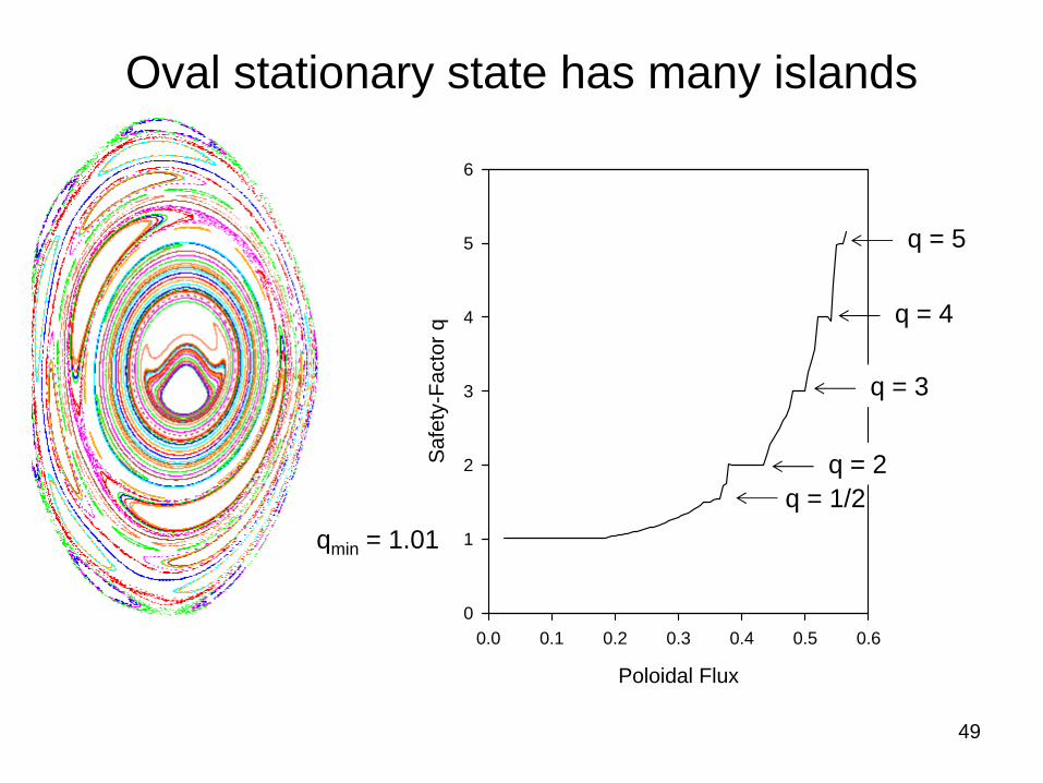
Oval stationary state has many islands
49
Poloidal Flux
0.0 0.1 0.2 0.3 0.4 0.5 0.6
Safe
ty-F
acto
r q
0
1
2
3
4
5
6
qmin = 1.01
q = 2q = 1/2
q = 3
q = 4
q = 5
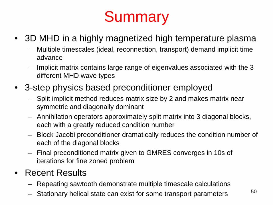
Summary• 3D MHD in a highly magnetized high temperature plasma
– Multiple timescales (ideal, reconnection, transport) demand implicit time advance
– Implicit matrix contains large range of eigenvalues associated with the 3 different MHD wave types
• 3-step physics based preconditioner employed– Split implicit method reduces matrix size by 2 and makes matrix near
symmetric and diagonally dominant– Annihilation operators approximately split matrix into 3 diagonal blocks,
each with a greatly reduced condition number– Block Jacobi preconditioner dramatically reduces the condition number of
each of the diagonal blocks– Final preconditioned matrix given to GMRES converges in 10s of
iterations for fine zoned problem
• Recent Results– Repeating sawtooth demonstrate multiple timescale calculations– Stationary helical state can exist for some transport parameters 50
Extra Viewgraphs
51
8/4/2011 52
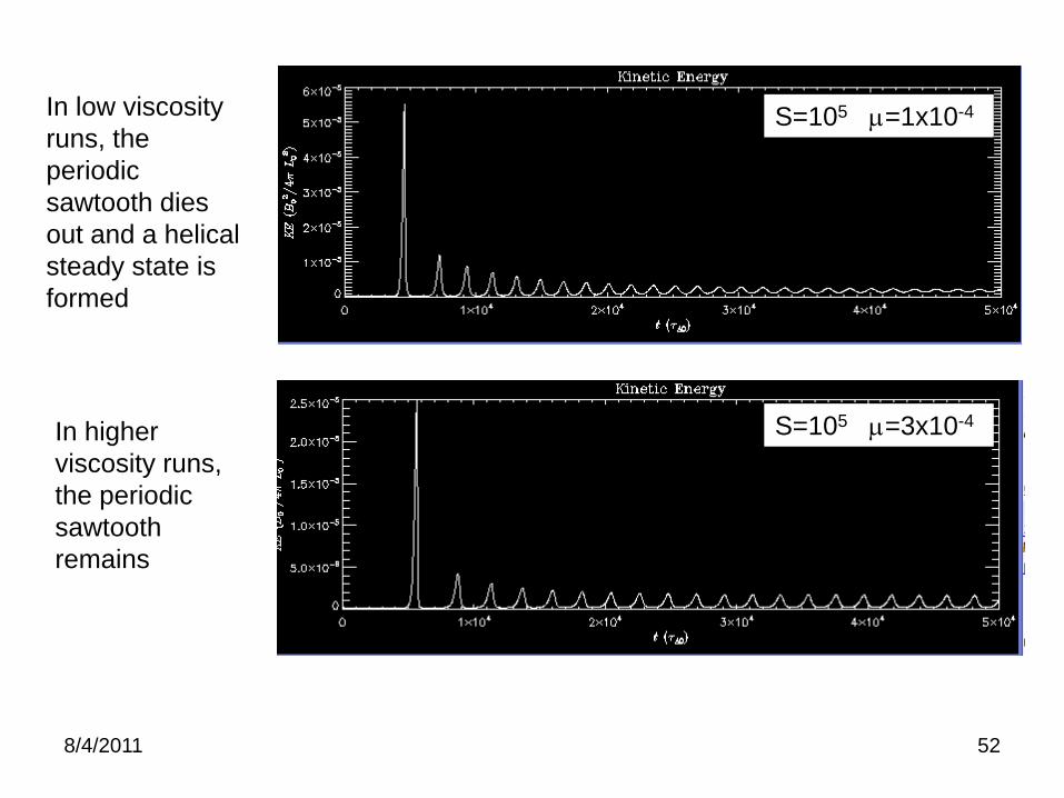
S=105 μ=1x10⁻⁴
S=105 μ=3x10⁻⁴
In low viscosity runs, the periodic sawtooth dies out and a helical steady state is formed
In higher viscosity runs, the periodic sawtooth remains
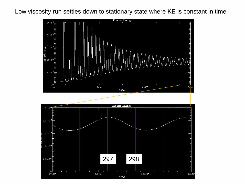
297 298
Low viscosity run settles down to stationary state where KE is constant in time
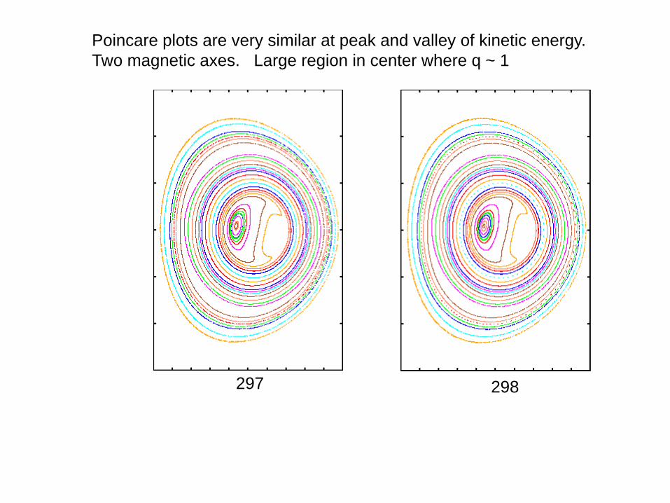
297 298
Poincare plots are very similar at peak and valley of kinetic energy. Two magnetic axes. Large region in center where q ~ 1
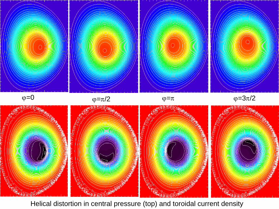
ϕ=0 ϕ=π/2 ϕ=π ϕ=3π/2
Helical distortion in central pressure (top) and toroidal current density
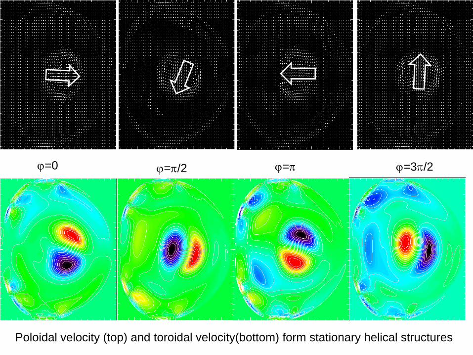
Poloidal velocity (top) and toroidal velocity(bottom) form stationary helical structures
ϕ=0 ϕ=π/2 ϕ=π ϕ=3π/2
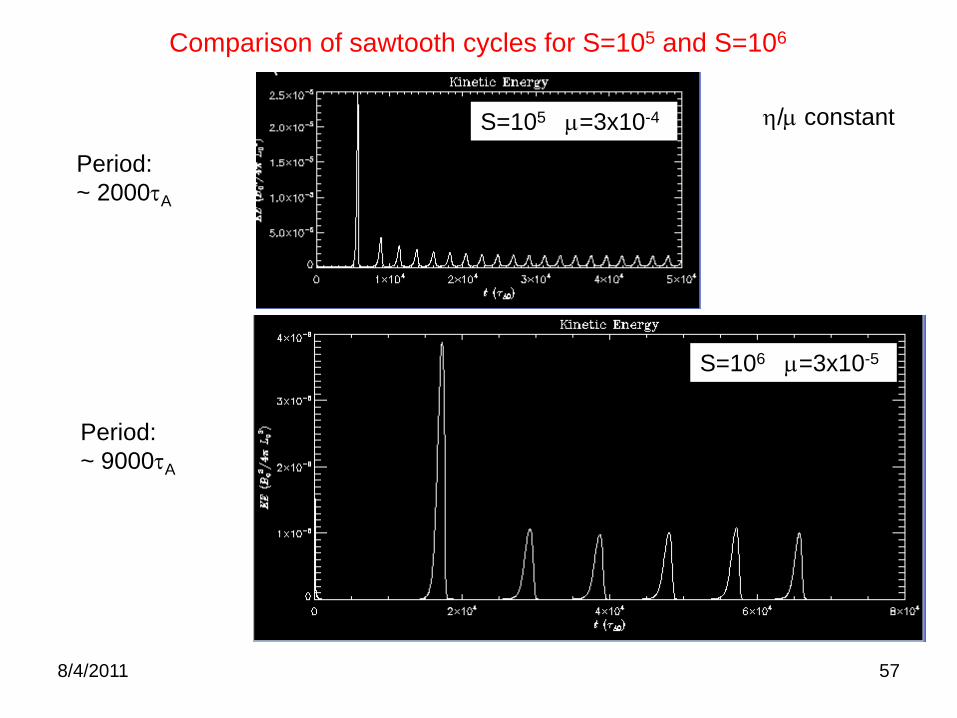
8/4/2011 57
S=105 μ=3x10⁻⁴
S=106 μ=3x10⁻⁵
Period:~ 2000τA
Period:~ 9000τA
Comparison of sawtooth cycles for S=105 and S=106
η/μ constant
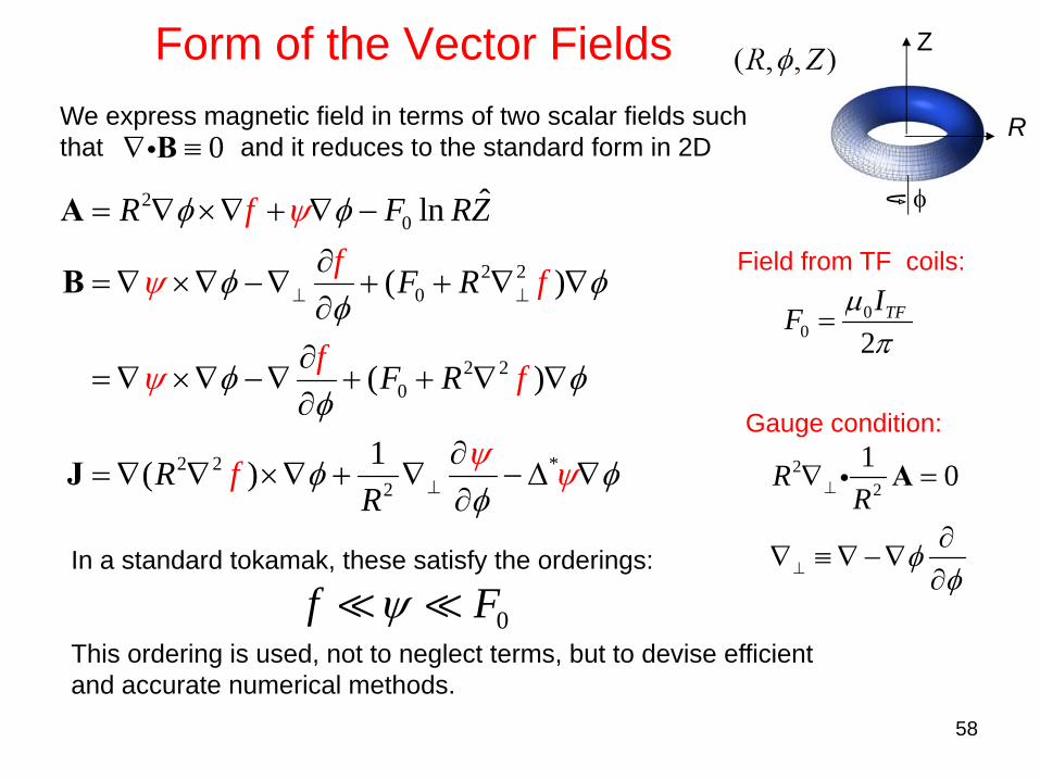
Form of the Vector Fields
58
In a standard tokamak, these satisfy the orderings:
This ordering is used, not to neglect terms, but to devise efficient and accurate numerical methods.
20
2 20
2 20
2 2 *2
ˆln
( )
( )
1( )
R F RZ
F R
F R
R
ff
R
f
f f
f
ψ
ψ
ψ
φ φ
φ φφ
φ φφ
φ ψ φφ
ψ
⊥ ⊥
⊥
= ∇ ×∇ + ∇ −∂
= ∇ ×∇ − ∇ + + ∇ ∇∂
∂= ∇ ×∇ − ∇ + + ∇ ∇
∂∂
= ∇ ∇ ×∇ + ∇ − Δ ∇∂
A
B
J
We express magnetic field in terms of two scalar fields such that and it reduces to the standard form in 2D
φ
Z
R
22
1 0RR
φφ
⊥
⊥
∇ =
∂∇ ≡ ∇ − ∇
∂
Ai
0f Fψ
0∇ ≡Bi
00 2
TFIF μπ
=
Field from TF coils:
Gauge condition:
Momentum Equation Projections
59
3 2 3 2(ME) (ME)i id R d Rτ ν ϕ τ ν ϕ⊥ ⊥∇ ∇ × → ∇ × ∇∫∫ ∫∫i i
3 2 3 2(ME) (ME)i id R d Rτ ν ϕ τ ν ϕ∇ → ∇∫∫ ∫∫i i
3 2 3 2(ME) (ME)i id R d Rτ ν τ ν− −⊥ ⊥− ∇ → ∇∫∫ ∫∫i i
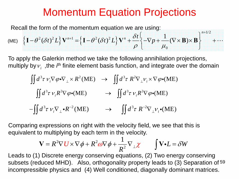
Recall the form of the momentum equation we are using:
(ME)
2 22
1UR R L WR
φ φω δχ⊥= ∇ ×∇ + ∇ + ∇ =∫V Vi
To apply the Galerkin method we take the following annihilation projections, multiply by ,the ith finite element basis function, and integrate over the domain
Comparing expressions on right with the velocity field, we see that this is equivalent to multiplying by each term in the velocity.
Leads to (1) Discrete energy conserving equations, (2) Two energy conserving subsets (reduced MHD). Also, orthogonality property leads to (3) Separation of incompressible physics and (4) Well conditioned, diagonally dominant matrices.
{ } { }1/2
2 2 1 2 2
0
1( ) ( ) ( )n
n n tt L t L pδθ δ θ δρ μ
+
+ ⎧ ⎫− = − + −∇ + ∇× × +⎨ ⎬
⎩ ⎭I V I V B B
iν