MULTIPLICATION AND INTEGRAL OPERATORS ON

SPACES OF ANALYTIC FUNCTIONS

A DISSERTATION SUBMITTED TO THE GRADUATE DIVISION OF THE

UNIVERSITY OF HAWAI‘I AT MANOA IN PARTIAL FULFILLMENT OF THE

REQUIREMENTS FOR THE DEGREE OF

DOCTOR OF PHILOSOPHY

IN

MATHEMATICS

DECEMBER 2010

By

Austin Maynard Anderson

Dissertation Committee:

Wayne Smith, Chairperson

George Csordas

Erik Guentner

Thomas Hoover

Lynne Wilkens

Acknowledgements

I would like to thank my adviser Wayne Smith for the countless hours he has devoted

to helping me with this work. I would also like to thank ARCS and the University

of Hawai‘i for their generous financial support. Finally, I am grateful to the many

professors at the University of Hawai‘i who have taught me and helped my career,

especially Monique Chyba, Adolf Mader, J. B. Nation, and Les Wilson.

ii

Abstract

We investigate operators on Banach spaces of analytic functions on the unit disk

D in the complex plane. The operator Tg, with symbol g(z) an analytic func-

tion on the disk, is defined by Tgf(z) =∫ z0f(w)g′(w) dw. The operator Tg and

its companion Sgf(z) =∫ z0f ′(w)g(w) dw are related to the multiplication operator

Mgf(z) = g(z)f(z), since integration by parts gives Mgf = f(0)g(0) + Tgf + Sgf.

Characterizing boundedness of Tg and Sg on the Dirichlet space, Bloch space,

and BMOA illuminates well known results on the multipliers (i.e., symbols g for

which Mg is bounded) of these spaces. The multipliers must satisfy two conditions,

which depend on the space. The operators Tg and Sg split the two conditions on

the multipliers. Mg is bounded only if both Sg and Tg are bounded, yet one of Sg

or Tg may be bounded when Mg is unbounded. We note a similar phenomenon on

the Hardy spaces Hp, 1 ≤ p < ∞, and Bergman spaces Ap. An open problem is to

distinguish the g for which Sg and Tg are bounded or compact on H∞, the space

of bounded analytic functions. We give partial results toward solving this problem,

including an example of a function g ∈ H∞ such that Tg is not bounded on H∞.

Finally, we study the symbols for which Tg and Sg have closed range on H2, Ap,

Bloch, and BMOA. Our main result regarding closed range operators is a characteri-

zation of g for which Sg has closed range on the Bloch space. We point out analogous

iii

results for H2 and the Bergman spaces. We also show Tg is never bounded below on

H2, Bloch, nor BMOA, but may be bounded below on Ap.

iv

Contents

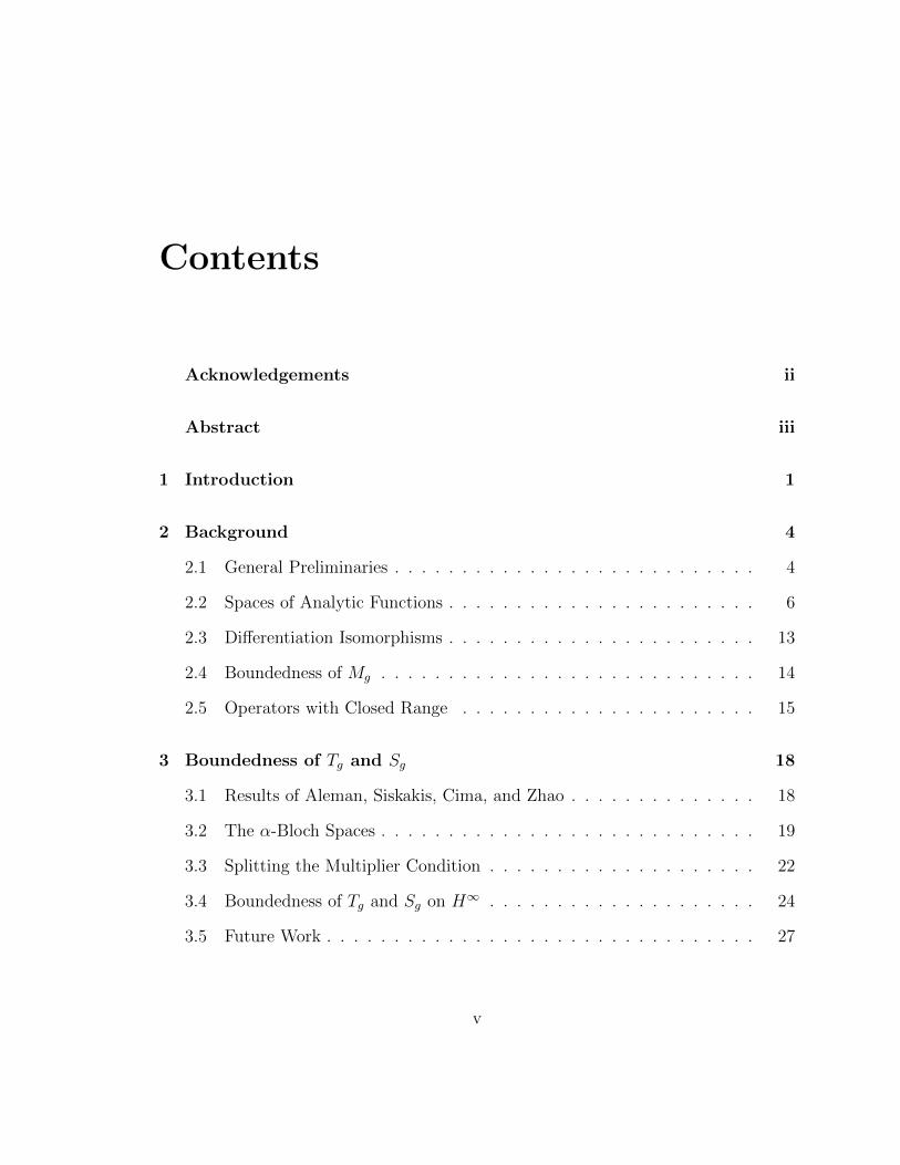
Acknowledgements ii

Abstract iii

1 Introduction 1

2 Background 4

2.1 General Preliminaries . . . . . . . . . . . . . . . . . . . . . . . . . . . 4

2.2 Spaces of Analytic Functions . . . . . . . . . . . . . . . . . . . . . . . 6

2.3 Differentiation Isomorphisms . . . . . . . . . . . . . . . . . . . . . . . 13

2.4 Boundedness of Mg . . . . . . . . . . . . . . . . . . . . . . . . . . . . 14

2.5 Operators with Closed Range . . . . . . . . . . . . . . . . . . . . . . 15

3 Boundedness of Tg and Sg 18

3.1 Results of Aleman, Siskakis, Cima, and Zhao . . . . . . . . . . . . . . 18

3.2 The α-Bloch Spaces . . . . . . . . . . . . . . . . . . . . . . . . . . . . 19

3.3 Splitting the Multiplier Condition . . . . . . . . . . . . . . . . . . . . 22

3.4 Boundedness of Tg and Sg on H∞ . . . . . . . . . . . . . . . . . . . . 24

3.5 Future Work . . . . . . . . . . . . . . . . . . . . . . . . . . . . . . . . 27

v

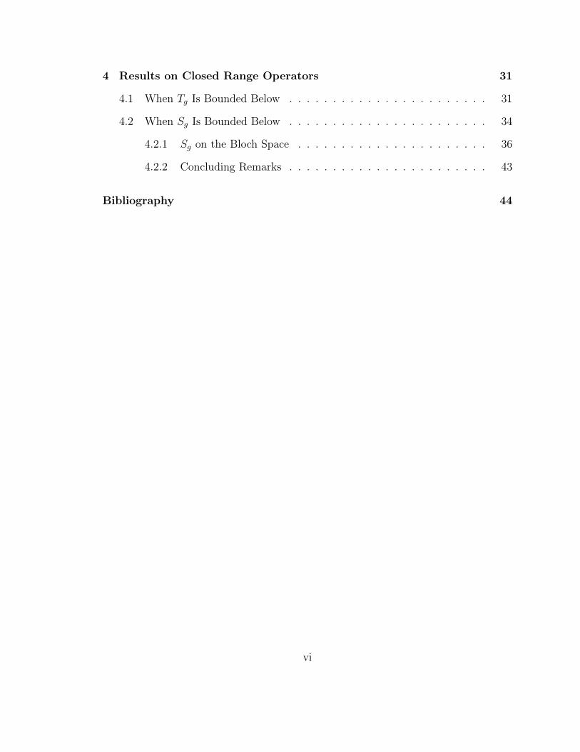
4 Results on Closed Range Operators 31

4.1 When Tg Is Bounded Below . . . . . . . . . . . . . . . . . . . . . . . 31

4.2 When Sg Is Bounded Below . . . . . . . . . . . . . . . . . . . . . . . 34

4.2.1 Sg on the Bloch Space . . . . . . . . . . . . . . . . . . . . . . 36

4.2.2 Concluding Remarks . . . . . . . . . . . . . . . . . . . . . . . 43

Bibliography 44

vi

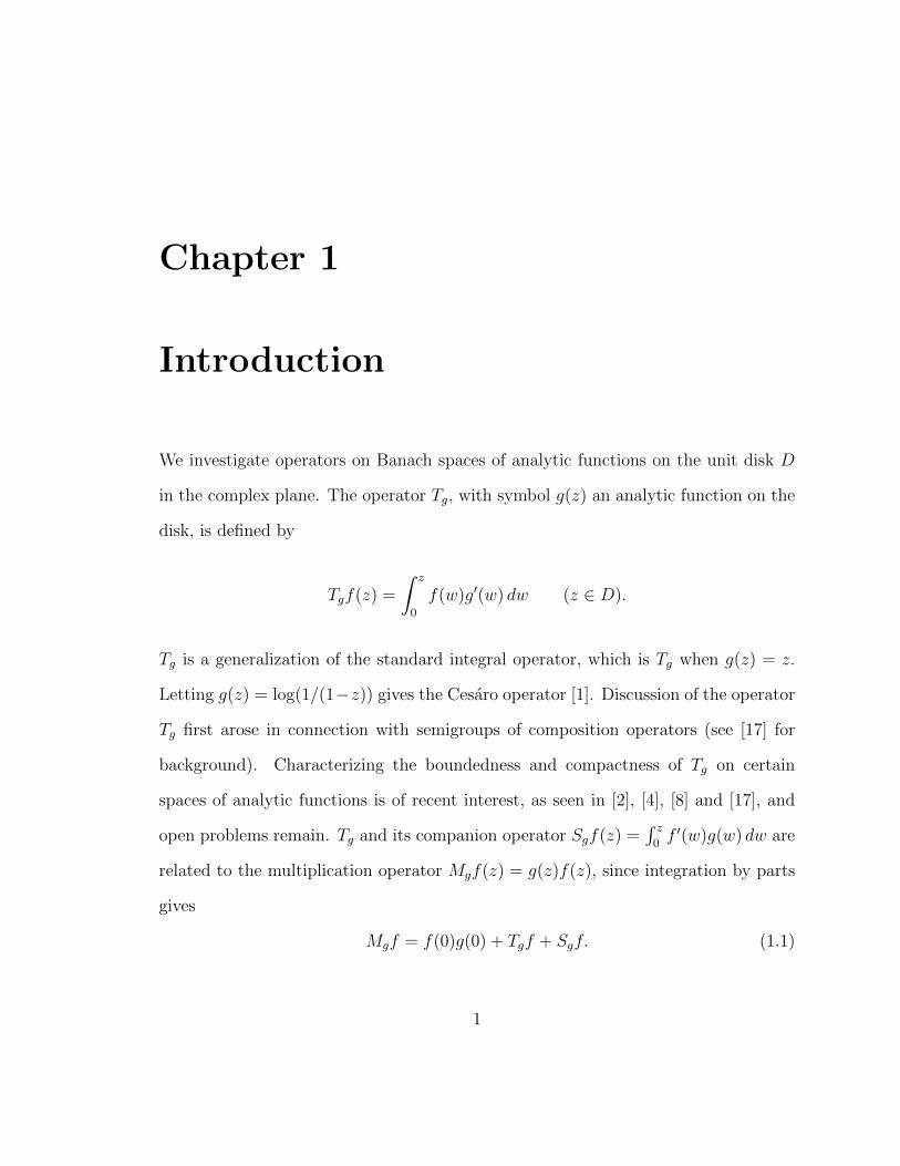
Chapter 1

Introduction

We investigate operators on Banach spaces of analytic functions on the unit disk D

in the complex plane. The operator Tg, with symbol g(z) an analytic function on the

disk, is defined by

Tgf(z) =

∫ z

0

f(w)g′(w) dw (z ∈ D).

Tg is a generalization of the standard integral operator, which is Tg when g(z) = z.

Letting g(z) = log(1/(1−z)) gives the Cesaro operator [1]. Discussion of the operator

Tg first arose in connection with semigroups of composition operators (see [17] for

background). Characterizing the boundedness and compactness of Tg on certain

spaces of analytic functions is of recent interest, as seen in [2], [4], [8] and [17], and

open problems remain. Tg and its companion operator Sgf(z) =∫ z0f ′(w)g(w) dw are

related to the multiplication operator Mgf(z) = g(z)f(z), since integration by parts

gives

Mgf = f(0)g(0) + Tgf + Sgf. (1.1)

1

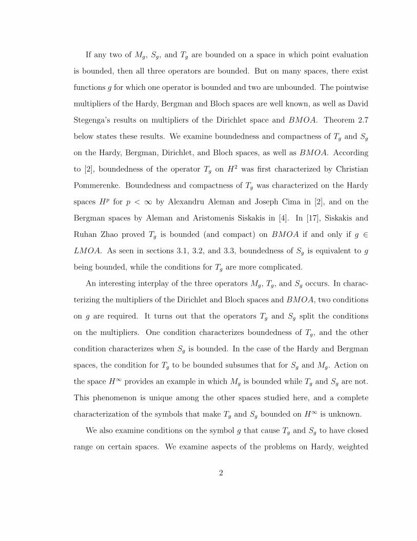
If any two of Mg, Sg, and Tg are bounded on a space in which point evaluation

is bounded, then all three operators are bounded. But on many spaces, there exist

functions g for which one operator is bounded and two are unbounded. The pointwise

multipliers of the Hardy, Bergman and Bloch spaces are well known, as well as David

Stegenga’s results on multipliers of the Dirichlet space and BMOA. Theorem 2.7

below states these results. We examine boundedness and compactness of Tg and Sg

on the Hardy, Bergman, Dirichlet, and Bloch spaces, as well as BMOA. According

to [2], boundedness of the operator Tg on H2 was first characterized by Christian

Pommerenke. Boundedness and compactness of Tg was characterized on the Hardy

spaces Hp for p < ∞ by Alexandru Aleman and Joseph Cima in [2], and on the

Bergman spaces by Aleman and Aristomenis Siskakis in [4]. In [17], Siskakis and

Ruhan Zhao proved Tg is bounded (and compact) on BMOA if and only if g ∈

LMOA. As seen in sections 3.1, 3.2, and 3.3, boundedness of Sg is equivalent to g

being bounded, while the conditions for Tg are more complicated.

An interesting interplay of the three operators Mg, Tg, and Sg occurs. In charac-

terizing the multipliers of the Dirichlet and Bloch spaces and BMOA, two conditions

on g are required. It turns out that the operators Tg and Sg split the conditions

on the multipliers. One condition characterizes boundedness of Tg, and the other

condition characterizes when Sg is bounded. In the case of the Hardy and Bergman

spaces, the condition for Tg to be bounded subsumes that for Sg and Mg. Action on

the space H∞ provides an example in which Mg is bounded while Tg and Sg are not.

This phenomenon is unique among the other spaces studied here, and a complete

characterization of the symbols that make Tg and Sg bounded on H∞ is unknown.

We also examine conditions on the symbol g that cause Tg and Sg to have closed

range on certain spaces. We examine aspects of the problems on Hardy, weighted

2

Bergman, and Bloch spaces, and BMOA. On the spaces studied, Tg and Sg have

closed range if and only if they are bounded below (Theorem 2.11). In Theorem 4.7,

we characterize the symbols g for which Sg is bounded below on the Bloch space. We

also point out analogous results for the Hardy space H2 and the weighted Bergman

spaces Apα for 1 ≤ p <∞, α > −1. In Theorem 4.1 we show the companion operator

Tg is never bounded below on H2, Bloch, nor BMOA. We subsequently mention an

example from [16] demonstrating Tg may be bounded below on Ap.

3

Chapter 2

Background

2.1 General Preliminaries

For two nonnegative quantities f and g, the notation f . g will mean there exists a

universal constant C such that f ≤ Cg. f ∼ g will mean f . g . f .

Let D = {z ∈ C : |z| < 1} be the unit disk in the complex plane and H(D) the

set of analytic functions on D.

Theorem 2.2 is a generalization of a result on multipliers of Banach spaces in which

point evaluation is a bounded linear functional. We state the result for multipliers

first.

Theorem 2.1. Let X be a Banach space of analytic functions on which point evalu-

ation is bounded for each point z ∈ D. Suppose Mg is bounded on X for some g ∈ X.

Then

|g(z)| ≤ ‖Mg‖.

The proof is similar to Theorem 2.2, so we omit it here. (See, e.g., [10, Lemma 11].)

4

Theorem 2.2. Let X and Y be Banach spaces of analytic functions, z ∈ D, and let

λz and λ′z be linear functionals defined by λzf = f(z) and λ′zf = f ′(z) for f ∈ X ∪Y .

Suppose λz and λ′z are bounded on X and Y .

(i) If Sg maps X boundedly into Y , then

|g(z)| ≤ ‖Sg‖‖λ′z‖Y‖λ′z‖X

.

(ii) If Tg maps X boundedly into Y , then

|g′(z)| ≤ ‖Tg‖‖λ′z‖Y‖λz‖X

.

Proof. Note that, for f ∈ X,

|f ′(z)||g(z)| = |λ′zSg(f)| ≤ ‖λ′z‖Y ‖Sg‖‖f‖X . (2.1)

Since

sup‖f‖X=1

|f ′(z)| = ‖λ′z‖X ,

taking the supremum of both sides of (2.1) over all f in X with norm 1 gives us

‖λ′z‖X |g(z)| ≤ ‖Sg‖‖λ′z‖Y .

Hence (i) holds. Similarly,

|f(z)||g′(z)| = |λ′zTg(f)| ≤ ‖λ′z‖Y ‖Tg‖‖f‖X .

5

Taking the supremum over {f ∈ X : ‖f‖X

= 1} , we get

‖λz‖X |g′(z)| ≤ ‖Tg‖‖λ′z‖Y .

This completes the proof.

When Y = X, we obtain the following corollary.

Corollary 2.3. If X is a Banach space of analytic functions on which point evaluation

of the derivative is a bounded linear functional, and Sg is bounded on X, then g is

bounded.

Corollary 2.3 will be used frequently below, because λ′z is bounded for each z ∈ D

on the spaces in which we are interested.

2.2 Spaces of Analytic Functions

We define several Banach spaces of analytic functions on which we will compare

various properties of Sg, Tg, and Mg. Zhu [21] is a good reference for background on

the spaces defined in this section.

For 1 ≤ p <∞, the Hardy space Hp on D is

{f ∈ H(D) : ‖f‖pp = sup0<r<1

∫ 2π

0

|f(reit)|p dt <∞}.

The space of bounded analytic functions on D is

H∞ = {f ∈ H(D) : ‖f‖∞ = supz∈D|f(z)| <∞}.

6

We define weighted Bergman spaces, for α > −1, 1 ≤ p <∞,

Apα = {f ∈ H(D) : ‖f‖pApα

=

∫D

|f(z)|p(1− |z|2)α dA(z) <∞},

where dA(z) refers to Lebesgue area measure on D. We denote the unweighted

Bergman space Ap = Ap0.

The Bloch space is

B = {f ∈ H(D) : ‖f‖B = supz∈D|f ′(z)|(1− |z|2) <∞}.

Note that ‖ ‖B is a semi-norm. The true norm is |f(0)|+‖f‖B, accounting for functions

differing by an additive constant. It is well known that H∞ a subspace of B, and

‖f‖B ≤ ‖f‖∞ for all f ∈ H∞ [21, Proposition 5.1]. For α > 0, the α-Bloch space Bα

and logarithmic Bloch space Bα,` are the following sets of analytic functions defined

on the disk:

Bα = {f ∈ H(D) : ‖f‖Bα = supz∈D|f ′(z)|(1− |z|2)α <∞},

Bα,` = {f ∈ H(D) : ‖f‖Bα,` = supz∈D|f ′(z)|(1− |z|2)α log

1

1− |z|<∞}.

Since B = B1, we define B` := B1,`. For 0 < α < 1, Bα are (analytic) Lipschitz class

spaces (see [9, Theorem 5.1]).

Define the conelike region with aperture α ∈ (0, 1) at eiθ to be

Γα(eiθ) =

{z ∈ D :

|eiθ − z|1− |z|

< α

}.

7

For a function f on D, define the nontangential limit of f at eiθ to be

f ∗(eiθ) = limz→eiθ

f(z) (z ∈ Γα(eiθ)),

provided the limit exists. If f ∈ H1, then the nontangential limit of f exists for

almost all eiθ ∈ ∂D (see [11, Theorem I.5.2]). In particular, we have the radial limit

limr→1− f(reiθ) = f ∗(eiθ) almost everywhere. When f is in H1, we define f(eiθ) =

f ∗(eiθ), so that f is defined on D except for a set of measure 0 in ∂D.

For a measurable complex-valued function ϕ defined on ∂D, and an arc I ⊆ ∂D,

define

ϕI =1

|I|

∫I

ϕ(eit) dt,

where |I| is the length of I, normalized so that |I| ≤ 1. The function ϕ has bounded

mean oscillation if

supI

1

|I|

∫I

|ϕ(eit)− ϕI |dt <∞,

as I ranges over all arcs in ∂D.

The space BMOA is the set of functions in H1 whose radial limit functions have

bounded mean oscillation. We define the semi-norm

‖f‖∗ = supI

1

|I|

∫I

|f(eit)− fI |dt,

so BMOA = {f ∈ H1 : ‖f‖∗ < ∞}. We assume f ∈ H1, although in fact, BMOA

is contained in H2. One way to see this is via the duality relations (H1)∗ ∼= BMOA

(see [21, Theorem 9.20]) and (Hp)∗ ∼= Hq, where 1/p+1/q = 1 (see [9, Theorem 7.3]).

Since H2 ⊂ H1, we have BMOA ∼= (H1)∗ ⊂ (H2)∗ ∼= H2. In fact, there exists C > 0

8

such that, for all f ∈ BMOA,

‖f‖2 ≤ C‖f‖∗. (2.2)

Note that H∞ is a subspace of BMOA, since for f ∈ H∞, the following calculation

shows

‖f‖∗ ≤ ‖f‖∞ : (2.3)

‖f‖∗ = supI

1

|I|

∫I

|f − fI |

≤ supI

(1

|I|

∫I

|f − fI |2)1/2

= supI

(1

|I|

∫I

(f − fI)(f − fI))1/2

= supI

(1

|I|

(∫I

|f |2 −∫I

ffI −∫I

ffI

)+ |fI |2

)1/2

= supI

((|f |2)I − |fI |2)1/2

≤ supI

((|f |2)I)1/2 ≤ ‖f‖∞.

The function f ∈ BMOA has vanishing mean oscillation if, for all ε > 0, there

exists δ > 0 such that |I| < δ implies

1

|I|

∫I

|f − fI | < ε.

The subspace of BMOA consisting of the functions with vanishing mean oscillation

is denoted VMOA. Another way we write the condition defining VMOA is

VMOA = {f ∈ BMOA : lim|I|→0

1

|I|

∫I

|f − fI | = 0}.

9

A noteworthy subspace of VMOA is those functions whose mean oscillation vanishes

as least as quickly as 1/ log(1/|I|). We define

LMOA = {f ∈ VMOA : lim|I|→0

log(1/|I|)|I|

∫I

|f − fI | <∞}.

A useful characterization of BMOA for our purposes involves Carleson measures.

For 1 ≤ p < ∞, a positive measure µ on D is a Carleson measure for Hp if there

exists C > 0 such that

∫D

|f |p dµ ≤ C‖f‖pp for all f ∈ Hp.

For an arc I ⊆ ∂D, define the Carleson rectangle associated with I to be

S(I) = {reiθ : 1− |I| < r < 1, eiθ ∈ I}.

For 1 ≤ p <∞, the measure µ is Carleson for Hp if and only if there exists C > 0 such

that µ(S(I)) ≤ C|I| for all arcs I ⊆ ∂D (a well-known result of Lennart Carleson,

see [11, Theorem II.3.9]). The smallest such C is called the Carleson constant for the

measure µ. Note that this characterization of Carleson measures is independent of p,

and it shows the Carleson measures for Hp are the same for all p (1 ≤ p <∞).

Define, for f ∈ H(D), dµf (z) = |f ′(z)|2(1− |z|2) dA(z). BMOA is the set of f ∈

H2 for which µf is Carleson for H2, and the BMOA semi-norm ‖f‖∗ is comparable

to the square root of the Carleson constant for µf (see [11, Theorem VI.3.4]). The

space VMOA is the set of f for which

lim|I|→0

µf (S(I))

|I|= 0.

10

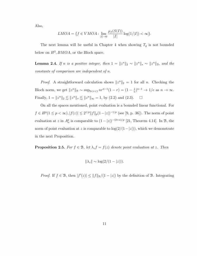
Also,

LMOA = {f ∈ VMOA : lim|I|→0

µf (S(I))

|I|log(1/|I|) <∞}.

The next lemma will be useful in Chapter 4 when showing Tg is not bounded

below on H2, BMOA, or the Bloch space.

Lemma 2.4. If n is a positive integer, then 1 = ‖zn‖2 ∼ ‖zn‖∗ ∼ ‖zn‖B, and the

constants of comparison are independent of n.

Proof. A straightforward calculation shows ‖zn‖2 = 1 for all n. Checking the

Bloch norm, we get ‖zn‖B ∼ sup0<r<1 nrn−1(1 − r) = (1 − 1

n)n−1 → 1/e as n → ∞.

Finally, 1 = ‖zn‖2 . ‖zn‖∗ . ‖zn‖∞ = 1, by (2.2) and (2.3).

On all the spaces mentioned, point evaluation is a bounded linear functional. For

f ∈ Hp(1 ≤ p <∞), |f(z)| ≤ 21/p‖f‖p(1−|z|)−1/p (see [9, p. 36]). The norm of point

evaluation at z in Apα is comparable to (1− |z|)−(2+α)/p [21, Theorem 4.14]. In B, the

norm of point evaluation at z is comparable to log(2/(1−|z|)), which we demonstrate

in the next Proposition.

Proposition 2.5. For f ∈ B, let λzf = f(z) denote point evaluation at z. Then

‖λz‖ ∼ log(2/(1− |z|)).

Proof. If f ∈ B, then |f ′(z)| ≤ ‖f‖B/(1− |z|) by the definition of B. Integrating

11

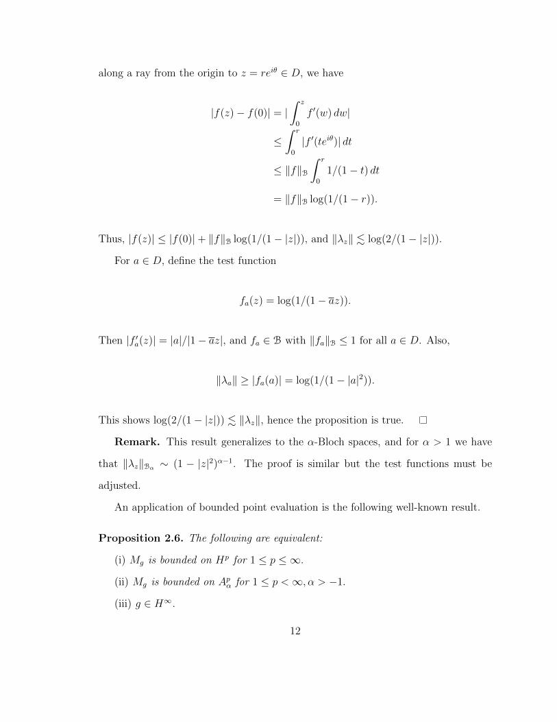
along a ray from the origin to z = reiθ ∈ D, we have

|f(z)− f(0)| = |∫ z

0

f ′(w) dw|

≤∫ r

0

|f ′(teiθ)| dt

≤ ‖f‖B∫ r

0

1/(1− t) dt

= ‖f‖B log(1/(1− r)).

Thus, |f(z)| ≤ |f(0)|+ ‖f‖B log(1/(1− |z|)), and ‖λz‖ . log(2/(1− |z|)).

For a ∈ D, define the test function

fa(z) = log(1/(1− az)).

Then |f ′a(z)| = |a|/|1− az|, and fa ∈ B with ‖fa‖B ≤ 1 for all a ∈ D. Also,

‖λa‖ ≥ |fa(a)| = log(1/(1− |a|2)).

This shows log(2/(1− |z|)) . ‖λz‖, hence the proposition is true.

Remark. This result generalizes to the α-Bloch spaces, and for α > 1 we have

that ‖λz‖Bα ∼ (1 − |z|2)α−1. The proof is similar but the test functions must be

adjusted.

An application of bounded point evaluation is the following well-known result.

Proposition 2.6. The following are equivalent:

(i) Mg is bounded on Hp for 1 ≤ p ≤ ∞.

(ii) Mg is bounded on Apα for 1 ≤ p <∞, α > −1.

(iii) g ∈ H∞.

12

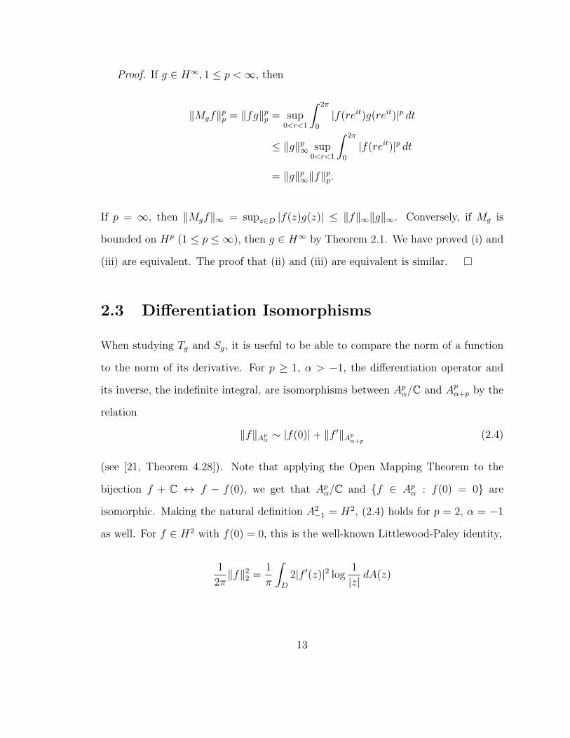
Proof. If g ∈ H∞, 1 ≤ p <∞, then

‖Mgf‖pp = ‖fg‖pp = sup0<r<1

∫ 2π

0

|f(reit)g(reit)|p dt

≤ ‖g‖p∞ sup0<r<1

∫ 2π

0

|f(reit)|p dt

= ‖g‖p∞‖f‖pp.

If p = ∞, then ‖Mgf‖∞ = supz∈D |f(z)g(z)| ≤ ‖f‖∞‖g‖∞. Conversely, if Mg is

bounded on Hp (1 ≤ p ≤ ∞), then g ∈ H∞ by Theorem 2.1. We have proved (i) and

(iii) are equivalent. The proof that (ii) and (iii) are equivalent is similar.

2.3 Differentiation Isomorphisms

When studying Tg and Sg, it is useful to be able to compare the norm of a function

to the norm of its derivative. For p ≥ 1, α > −1, the differentiation operator and

its inverse, the indefinite integral, are isomorphisms between Apα/C and Apα+p by the

relation

‖f‖Apα ∼ |f(0)|+ ‖f ′‖Apα+p (2.4)

(see [21, Theorem 4.28]). Note that applying the Open Mapping Theorem to the

bijection f + C ↔ f − f(0), we get that Apα/C and {f ∈ Apα : f(0) = 0} are

isomorphic. Making the natural definition A2−1 = H2, (2.4) holds for p = 2, α = −1

as well. For f ∈ H2 with f(0) = 0, this is the well-known Littlewood-Paley identity,

1

2π‖f‖22 =

1

π

∫D

2|f ′(z)|2 log1

|z|dA(z)

13

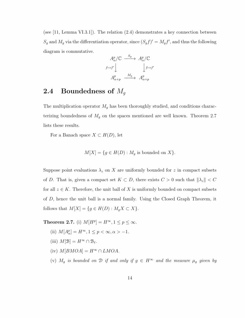
(see [11, Lemma VI.3.1]). The relation (2.4) demonstrates a key connection between

Sg andMg via the differentiation operator, since (Sgf)′ = Mgf′, and thus the following

diagram is commutative.

Apα/CSg−−−→ Apα/C

f 7→f ′y yf 7→f ′

Apα+pMg−−−→ Apα+p

2.4 Boundedness of Mg

The multiplication operator Mg has been thoroughly studied, and conditions charac-

terizing boundedness of Mg on the spaces mentioned are well known. Theorem 2.7

lists these results.

For a Banach space X ⊂ H(D), let

M [X] = {g ∈ H(D) : Mg is bounded on X}.

Suppose point evaluations λz on X are uniformly bounded for z in compact subsets

of D. That is, given a compact set K ⊂ D, there exists C > 0 such that ‖λz‖ < C

for all z ∈ K. Therefore, the unit ball of X is uniformly bounded on compact subsets

of D, hence the unit ball is a normal family. Using the Closed Graph Theorem, it

follows that M [X] = {g ∈ H(D) : MgX ⊂ X}.

Theorem 2.7. (i) M [Hp] = H∞, 1 ≤ p ≤ ∞.

(ii) M [Apα] = H∞, 1 ≤ p <∞, α > −1.

(iii) M [B] = H∞ ∩B`.

(iv) M [BMOA] = H∞ ∩ LMOA.

(v) Mg is bounded on D if and only if g ∈ H∞ and the measure µg given by

14

dµg(z) = |g′(z)|2dA(z) is a Carleson measure for D.

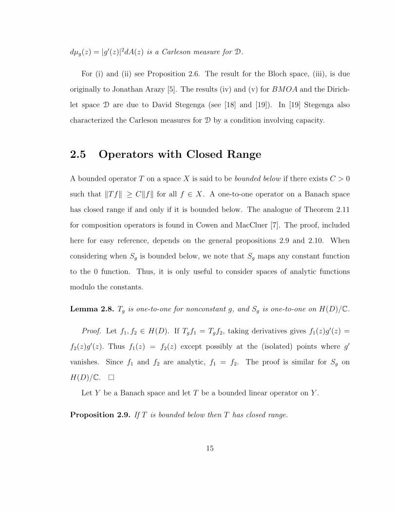
For (i) and (ii) see Proposition 2.6. The result for the Bloch space, (iii), is due

originally to Jonathan Arazy [5]. The results (iv) and (v) for BMOA and the Dirich-

let space D are due to David Stegenga (see [18] and [19]). In [19] Stegenga also

characterized the Carleson measures for D by a condition involving capacity.

2.5 Operators with Closed Range

A bounded operator T on a space X is said to be bounded below if there exists C > 0

such that ‖Tf‖ ≥ C‖f‖ for all f ∈ X. A one-to-one operator on a Banach space

has closed range if and only if it is bounded below. The analogue of Theorem 2.11

for composition operators is found in Cowen and MacCluer [7]. The proof, included

here for easy reference, depends on the general propositions 2.9 and 2.10. When

considering when Sg is bounded below, we note that Sg maps any constant function

to the 0 function. Thus, it is only useful to consider spaces of analytic functions

modulo the constants.

Lemma 2.8. Tg is one-to-one for nonconstant g, and Sg is one-to-one on H(D)/C.

Proof. Let f1, f2 ∈ H(D). If Tgf1 = Tgf2, taking derivatives gives f1(z)g′(z) =

f2(z)g′(z). Thus f1(z) = f2(z) except possibly at the (isolated) points where g′

vanishes. Since f1 and f2 are analytic, f1 = f2. The proof is similar for Sg on

H(D)/C.

Let Y be a Banach space and let T be a bounded linear operator on Y .

Proposition 2.9. If T is bounded below then T has closed range.

15

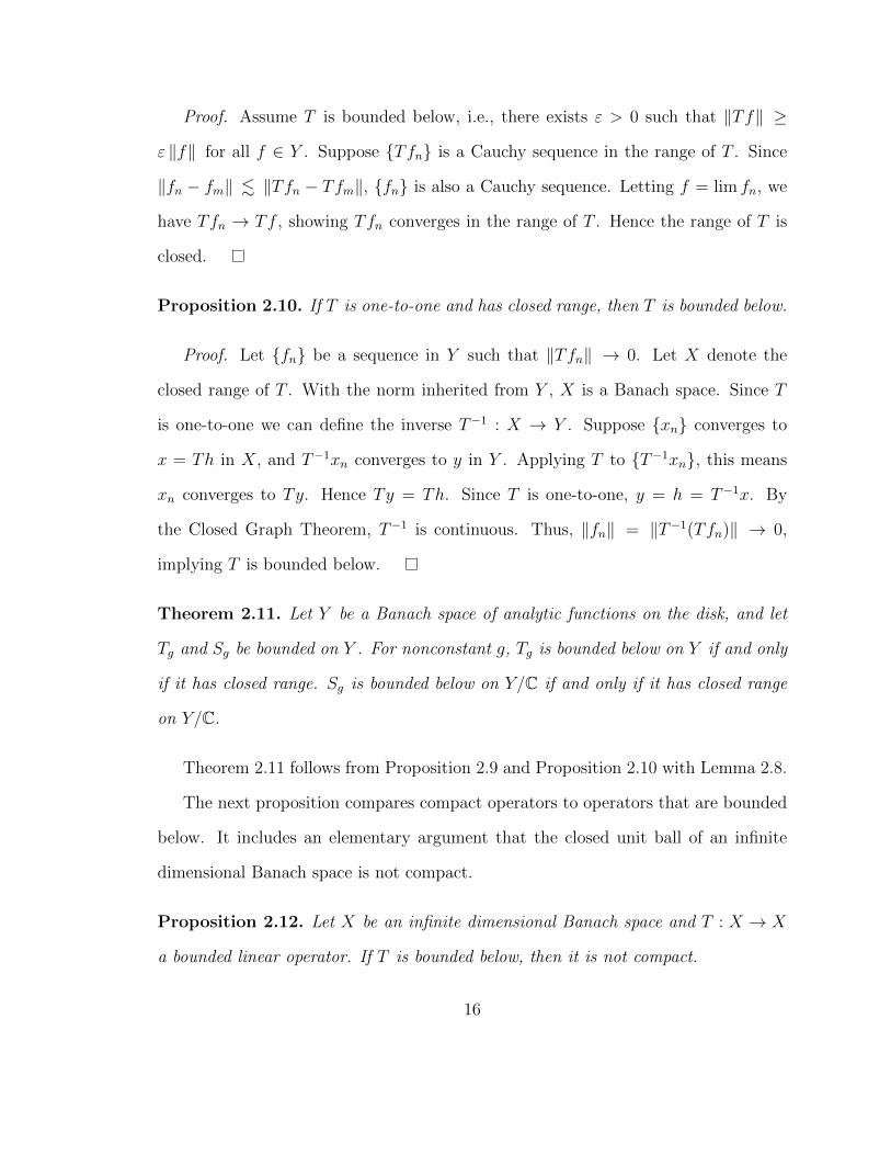
Proof. Assume T is bounded below, i.e., there exists ε > 0 such that ‖Tf‖ ≥

ε ‖f‖ for all f ∈ Y . Suppose {Tfn} is a Cauchy sequence in the range of T . Since

‖fn − fm‖ . ‖Tfn − Tfm‖, {fn} is also a Cauchy sequence. Letting f = lim fn, we

have Tfn → Tf , showing Tfn converges in the range of T . Hence the range of T is

closed.

Proposition 2.10. If T is one-to-one and has closed range, then T is bounded below.

Proof. Let {fn} be a sequence in Y such that ‖Tfn‖ → 0. Let X denote the

closed range of T . With the norm inherited from Y , X is a Banach space. Since T

is one-to-one we can define the inverse T−1 : X → Y . Suppose {xn} converges to

x = Th in X, and T−1xn converges to y in Y . Applying T to {T−1xn}, this means

xn converges to Ty. Hence Ty = Th. Since T is one-to-one, y = h = T−1x. By

the Closed Graph Theorem, T−1 is continuous. Thus, ‖fn‖ = ‖T−1(Tfn)‖ → 0,

implying T is bounded below.

Theorem 2.11. Let Y be a Banach space of analytic functions on the disk, and let

Tg and Sg be bounded on Y . For nonconstant g, Tg is bounded below on Y if and only

if it has closed range. Sg is bounded below on Y/C if and only if it has closed range

on Y/C.

Theorem 2.11 follows from Proposition 2.9 and Proposition 2.10 with Lemma 2.8.

The next proposition compares compact operators to operators that are bounded

below. It includes an elementary argument that the closed unit ball of an infinite

dimensional Banach space is not compact.

Proposition 2.12. Let X be an infinite dimensional Banach space and T : X → X

a bounded linear operator. If T is bounded below, then it is not compact.

16

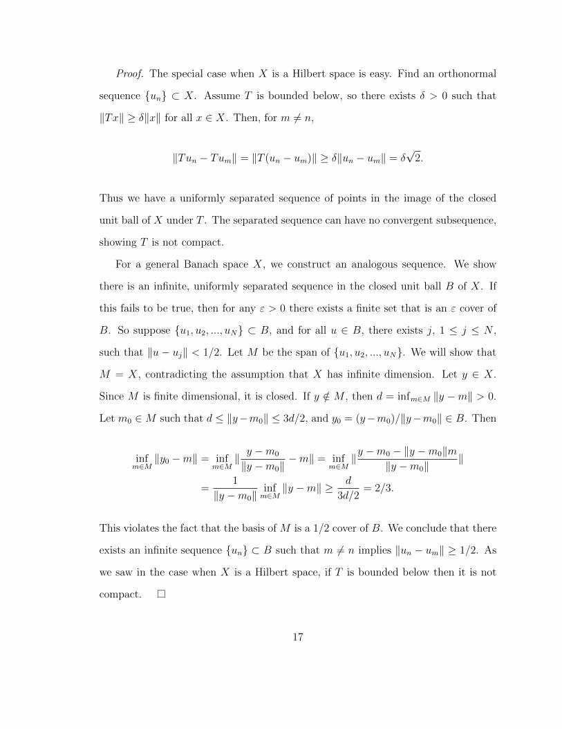
Proof. The special case when X is a Hilbert space is easy. Find an orthonormal

sequence {un} ⊂ X. Assume T is bounded below, so there exists δ > 0 such that

‖Tx‖ ≥ δ‖x‖ for all x ∈ X. Then, for m 6= n,

‖Tun − Tum‖ = ‖T (un − um)‖ ≥ δ‖un − um‖ = δ√

2.

Thus we have a uniformly separated sequence of points in the image of the closed

unit ball of X under T . The separated sequence can have no convergent subsequence,

showing T is not compact.

For a general Banach space X, we construct an analogous sequence. We show

there is an infinite, uniformly separated sequence in the closed unit ball B of X. If

this fails to be true, then for any ε > 0 there exists a finite set that is an ε cover of

B. So suppose {u1, u2, ..., uN} ⊂ B, and for all u ∈ B, there exists j, 1 ≤ j ≤ N ,

such that ‖u− uj‖ < 1/2. Let M be the span of {u1, u2, ..., uN}. We will show that

M = X, contradicting the assumption that X has infinite dimension. Let y ∈ X.

Since M is finite dimensional, it is closed. If y /∈ M , then d = infm∈M ‖y −m‖ > 0.

Let m0 ∈M such that d ≤ ‖y−m0‖ ≤ 3d/2, and y0 = (y−m0)/‖y−m0‖ ∈ B. Then

infm∈M

‖y0 −m‖ = infm∈M

‖ y −m0

‖y −m0‖−m‖ = inf

m∈M‖y −m0 − ‖y −m0‖m

‖y −m0‖‖

=1

‖y −m0‖infm∈M

‖y −m‖ ≥ d

3d/2= 2/3.

This violates the fact that the basis of M is a 1/2 cover of B. We conclude that there

exists an infinite sequence {un} ⊂ B such that m 6= n implies ‖un − um‖ ≥ 1/2. As

we saw in the case when X is a Hilbert space, if T is bounded below then it is not

compact.

17

Chapter 3

Boundedness of Tg and Sg

3.1 Results of Aleman, Siskakis, Cima, and Zhao

Alexandru Aleman and Aristomenis Siskakis characterized boundedness and com-

pactness of Tg on Hp for 1 ≤ p < ∞ in [3] (Theorem 3.1 below). The dual of H1

is BMOA ([21, Theorem 9.20]), and the dual of the Bergman space A1 is the Bloch

space ([21, Theorem 5.3]). Hence, in light of duality, Theorem 3.2 is an analogue

for the Bergman spaces of Theorem 3.1. Theorem 3.2 was proved by Aleman and

Siskakis in [4]. Theorem 3.3 was established by Siskakis and Ruhan Zhao in [17].

Theorem 3.1. (Aleman and Siskakis [3]) For 1 ≤ p < ∞, Tg is bounded [compact]

on Hp if and only if g ∈ BMOA [VMOA].

Theorem 3.2. (Aleman and Siskakis [4]) For p ≥ 1, Tg is bounded [compact] on Ap

if and only if g ∈ B [B0].

Theorem 3.3. (Siskakis and Zhao [17]) Tg is bounded on BMOA if and only if

g ∈ LMOA.

18

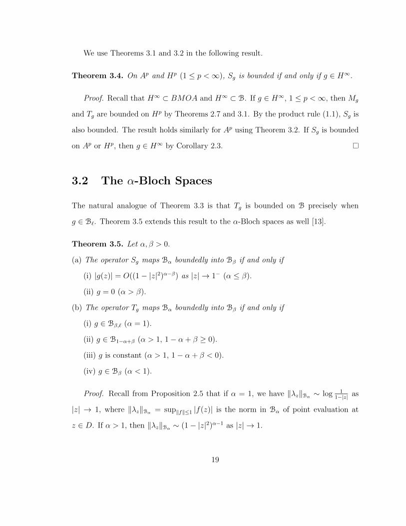
We use Theorems 3.1 and 3.2 in the following result.

Theorem 3.4. On Ap and Hp (1 ≤ p <∞), Sg is bounded if and only if g ∈ H∞.

Proof. Recall that H∞ ⊂ BMOA and H∞ ⊂ B. If g ∈ H∞, 1 ≤ p <∞, then Mg

and Tg are bounded on Hp by Theorems 2.7 and 3.1. By the product rule (1.1), Sg is

also bounded. The result holds similarly for Ap using Theorem 3.2. If Sg is bounded

on Ap or Hp, then g ∈ H∞ by Corollary 2.3.

3.2 The α-Bloch Spaces

The natural analogue of Theorem 3.3 is that Tg is bounded on B precisely when

g ∈ B`. Theorem 3.5 extends this result to the α-Bloch spaces as well [13].

Theorem 3.5. Let α, β > 0.

(a) The operator Sg maps Bα boundedly into Bβ if and only if

(i) |g(z)| = O((1− |z|2)α−β) as |z| → 1− (α ≤ β).

(ii) g = 0 (α > β).

(b) The operator Tg maps Bα boundedly into Bβ if and only if

(i) g ∈ Bβ,` (α = 1).

(ii) g ∈ B1−α+β (α > 1, 1− α + β ≥ 0).

(iii) g is constant (α > 1, 1− α + β < 0).

(iv) g ∈ Bβ (α < 1).

Proof. Recall from Proposition 2.5 that if α = 1, we have ‖λz‖Bα ∼ log 11−|z| as

|z| → 1, where ‖λz‖Bα = sup‖f‖≤1 |f(z)| is the norm in Bα of point evaluation at

z ∈ D. If α > 1, then ‖λz‖Bα ∼ (1− |z|2)α−1 as |z| → 1.

19

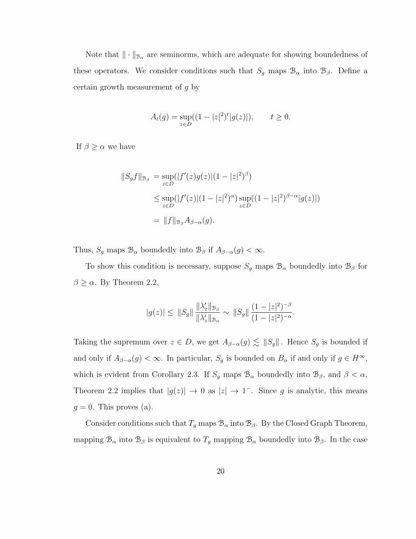
Note that ‖ · ‖Bα are seminorms, which are adequate for showing boundedness of

these operators. We consider conditions such that Sg maps Bα into Bβ. Define a

certain growth measurement of g by

At(g) = supz∈D

((1− |z|2)t|g(z)|), t ≥ 0.

If β ≥ α we have

‖Sgf‖Bβ = supz∈D

(|f ′(z)g(z)|(1− |z|2)β)

≤ supz∈D

(|f ′(z)|(1− |z|2)α) supz∈D

((1− |z|2)β−α|g(z)|)

= ‖f‖BβAβ−α(g).

Thus, Sg maps Bα boundedly into Bβ if Aβ−α(g) <∞.

To show this condition is necessary, suppose Sg maps Bα boundedly into Bβ for

β ≥ α. By Theorem 2.2,

|g(z)| ≤ ‖Sg‖‖λ′z‖Bβ‖λ′z‖Bα

∼ ‖Sg‖(1− |z|2)−β

(1− |z|2)−α.

Taking the supremum over z ∈ D, we get Aβ−α(g) . ‖Sg‖ . Hence Sg is bounded if

and only if Aβ−α(g) <∞. In particular, Sg is bounded on Bα if and only if g ∈ H∞,

which is evident from Corollary 2.3. If Sg maps Bα boundedly into Bβ, and β < α,

Theorem 2.2 implies that |g(z)| → 0 as |z| → 1−. Since g is analytic, this means

g = 0. This proves (a).

Consider conditions such that Tg maps Bα into Bβ. By the Closed Graph Theorem,

mapping Bα into Bβ is equivalent to Tg mapping Bα boundedly into Bβ. In the case

20

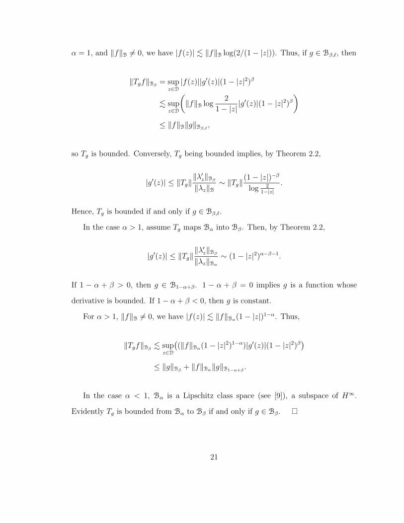
α = 1, and ‖f‖B 6= 0, we have |f(z)| . ‖f‖B log(2/(1− |z|)). Thus, if g ∈ Bβ,`, then

‖Tgf‖Bβ = supz∈D|f(z)||g′(z)|(1− |z|2)β

. supz∈D

(‖f‖B log

2

1− |z||g′(z)|(1− |z|2)β

)≤ ‖f‖B‖g‖Bβ,` ,

so Tg is bounded. Conversely, Tg being bounded implies, by Theorem 2.2,

|g′(z)| ≤ ‖Tg‖‖λ′z‖Bβ‖λz‖B

∼ ‖Tg‖(1− |z|)−β

log 21−|z|

.

Hence, Tg is bounded if and only if g ∈ Bβ,`.

In the case α > 1, assume Tg maps Bα into Bβ. Then, by Theorem 2.2,

|g′(z)| ≤ ‖Tg‖‖λ′z‖Bβ‖λz‖Bα

∼ (1− |z|2)α−β−1.

If 1 − α + β > 0, then g ∈ B1−α+β. 1 − α + β = 0 implies g is a function whose

derivative is bounded. If 1− α + β < 0, then g is constant.

For α > 1, ‖f‖B 6= 0, we have |f(z)| . ‖f‖Bα(1− |z|)1−α. Thus,

‖Tgf‖Bβ . supz∈D

((‖f‖Bα(1− |z|2)1−α)|g′(z)|(1− |z|2)β

)≤ ‖g‖Bβ + ‖f‖Bα‖g‖B1−α+β .

In the case α < 1, Bα is a Lipschitz class space (see [9]), a subspace of H∞.

Evidently Tg is bounded from Bα to Bβ if and only if g ∈ Bβ.

21

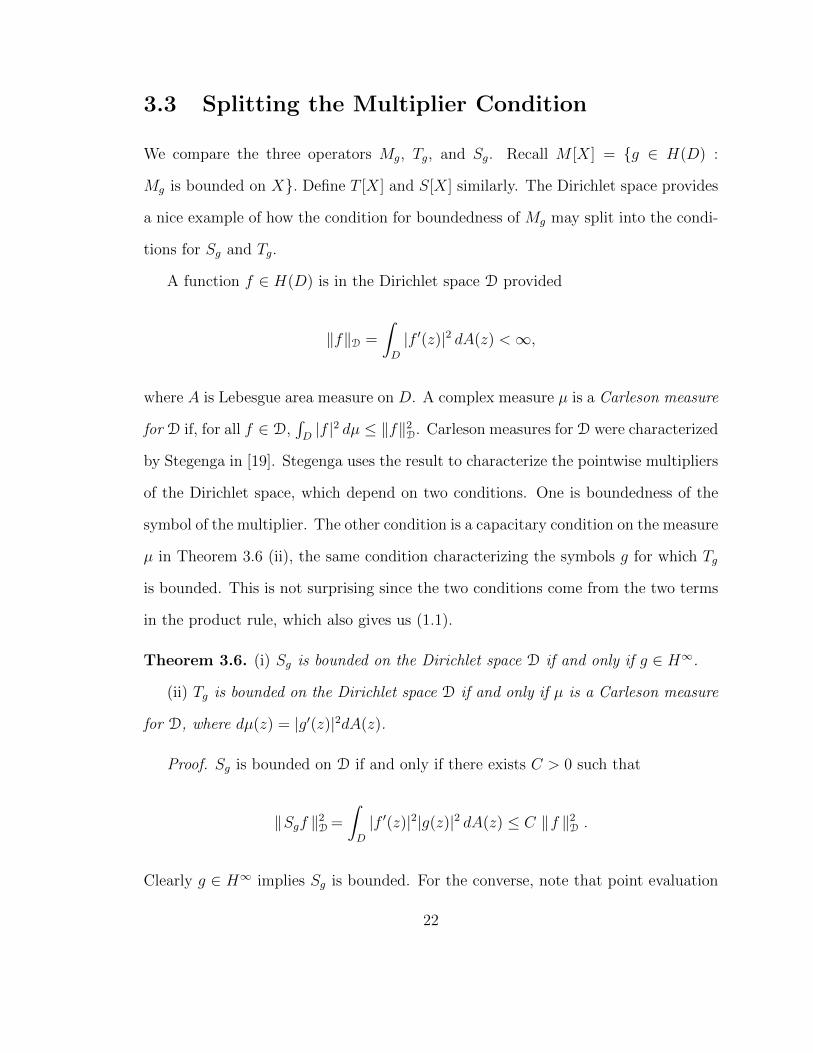
3.3 Splitting the Multiplier Condition

We compare the three operators Mg, Tg, and Sg. Recall M [X] = {g ∈ H(D) :

Mg is bounded on X}. Define T [X] and S[X] similarly. The Dirichlet space provides

a nice example of how the condition for boundedness of Mg may split into the condi-

tions for Sg and Tg.

A function f ∈ H(D) is in the Dirichlet space D provided

‖f‖D =

∫D

|f ′(z)|2 dA(z) <∞,

where A is Lebesgue area measure on D. A complex measure µ is a Carleson measure

for D if, for all f ∈ D,∫D|f |2 dµ ≤ ‖f‖2D. Carleson measures for D were characterized

by Stegenga in [19]. Stegenga uses the result to characterize the pointwise multipliers

of the Dirichlet space, which depend on two conditions. One is boundedness of the

symbol of the multiplier. The other condition is a capacitary condition on the measure

µ in Theorem 3.6 (ii), the same condition characterizing the symbols g for which Tg

is bounded. This is not surprising since the two conditions come from the two terms

in the product rule, which also gives us (1.1).

Theorem 3.6. (i) Sg is bounded on the Dirichlet space D if and only if g ∈ H∞.

(ii) Tg is bounded on the Dirichlet space D if and only if µ is a Carleson measure

for D, where dµ(z) = |g′(z)|2dA(z).

Proof. Sg is bounded on D if and only if there exists C > 0 such that

‖Sgf ‖2D =

∫D

|f ′(z)|2|g(z)|2 dA(z) ≤ C ‖f ‖2D .

Clearly g ∈ H∞ implies Sg is bounded. For the converse, note that point evaluation

22

of the derivative in D is analogous to point evaluation in A2, and ‖λ′z‖D ∼ ‖λz‖A2 .

Thus, Corollary 2.3 applies, proving (i).

Tg is bounded on D if and only if there exists C > 0 such that

‖Tgf ‖2D=

∫D

|f(z)|2|g′(z)|2 dA(z) ≤ C ‖f ‖2D .

This is precisely the statement in (ii).

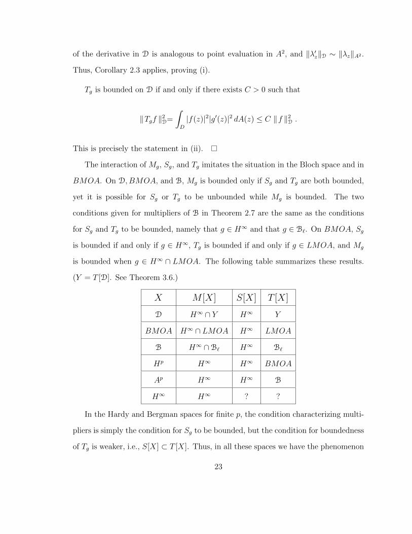
The interaction of Mg, Sg, and Tg imitates the situation in the Bloch space and in

BMOA. On D, BMOA, and B, Mg is bounded only if Sg and Tg are both bounded,

yet it is possible for Sg or Tg to be unbounded while Mg is bounded. The two

conditions given for multipliers of B in Theorem 2.7 are the same as the conditions

for Sg and Tg to be bounded, namely that g ∈ H∞ and that g ∈ B`. On BMOA, Sg

is bounded if and only if g ∈ H∞, Tg is bounded if and only if g ∈ LMOA, and Mg

is bounded when g ∈ H∞ ∩ LMOA. The following table summarizes these results.

(Y = T [D]. See Theorem 3.6.)

X M [X] S[X] T [X]

D H∞ ∩ Y H∞ Y

BMOA H∞ ∩ LMOA H∞ LMOA

B H∞ ∩B` H∞ B`

Hp H∞ H∞ BMOA

Ap H∞ H∞ B

H∞ H∞ ? ?

In the Hardy and Bergman spaces for finite p, the condition characterizing multi-

pliers is simply the condition for Sg to be bounded, but the condition for boundedness

of Tg is weaker, i.e., S[X] ⊂ T [X]. Thus, in all these spaces we have the phenomenon

23

that boundedness of the multiplication operator Mg is equivalent to boundedness of

both Sg and Tg. As we will see in Section 3.4 below, this phenomenon fails for the op-

erators acting on H∞. The question marks in the table represent unsolved problems,

but some discussion and partial results will be presented.

3.4 Boundedness of Tg and Sg on H∞

It is trivial that M [H∞] = H∞, i.e., the multipliers of H∞ are precisely the functions

in H∞ themselves. Such is not the case for Tg and Sg, and characterizing boundedness

of these operators on H∞ is an open problem. The following proposition gives a

necessary condition for Tg and Sg to be bounded on H∞.

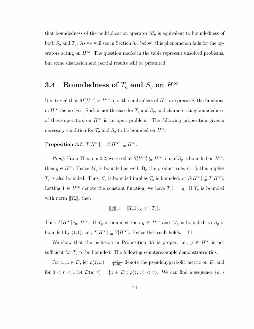
Proposition 3.7. T [H∞] = S[H∞] ⊆ H∞.

Proof. From Theorem 2.2, we see that S[H∞] ⊆ H∞, i.e., if Sg is bounded on H∞,

then g ∈ H∞. Hence Mg is bounded as well. By the product rule, (1.1), this implies

Tg is also bounded. Thus, Sg is bounded implies Tg is bounded, or S[H∞] ⊆ T [H∞].

Letting 1 ∈ H∞ denote the constant function, we have Tg1 = g. If Tg is bounded

with norm ‖Tg‖, then

‖g‖∞ = ‖Tg1‖∞ ≤ ‖Tg‖.

Thus T [H∞] ⊆ H∞. If Tg is bounded then g ∈ H∞ and Mg is bounded, so Sg is

bounded by (1.1), i.e., T [H∞] ⊆ S[H∞]. Hence the result holds.

We show that the inclusion in Proposition 3.7 is proper, i.e., g ∈ H∞ is not

sufficient for Tg to be bounded. The following counterexample demonstrates this.

For w, z ∈ D, let ρ(z, w) = |w−z||1−wz| denote the pseudohyperbolic metric on D, and

for 0 < r < 1 let D(w, r) = {z ∈ D : ρ(z, w) < r}. We can find a sequence {an}

24

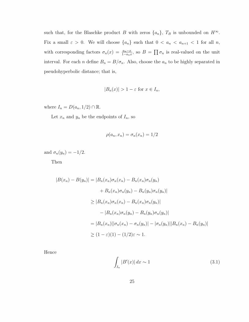
such that, for the Blaschke product B with zeros {an}, TB is unbounded on H∞.

Fix a small ε > 0. We will choose {an} such that 0 < an < an+1 < 1 for all n,

with corresponding factors σn(x) = an−x1−anx , so B =

∏σn is real-valued on the unit

interval. For each n define Bn = B/σn. Also, choose the an to be highly separated in

pseudohyperbolic distance; that is,

|Bn(x)| > 1− ε for x ∈ In,

where In = D(an, 1/2) ∩ R.

Let xn and yn be the endpoints of In, so

ρ(an, xn) = σn(xn) = 1/2

and σn(yn) = −1/2.

Then

|B(xn)−B(yn)| = |Bn(xn)σn(xn)−Bn(xn)σn(yn)

+Bn(xn)σn(yn)−Bn(yn)σn(yn)|

≥ |Bn(xn)σn(xn)−Bn(xn)σn(yn)|

− |Bn(xn)σn(yn)−Bn(yn)σn(yn)|

= |Bn(xn)||σn(xn)− σn(yn)| − |σn(yn)||Bn(xn)−Bn(yn)|

≥ (1− ε)(1)− (1/2)ε ∼ 1.

Hence ∫In

|B′(x)| dx ∼ 1 (3.1)

25

for all n.

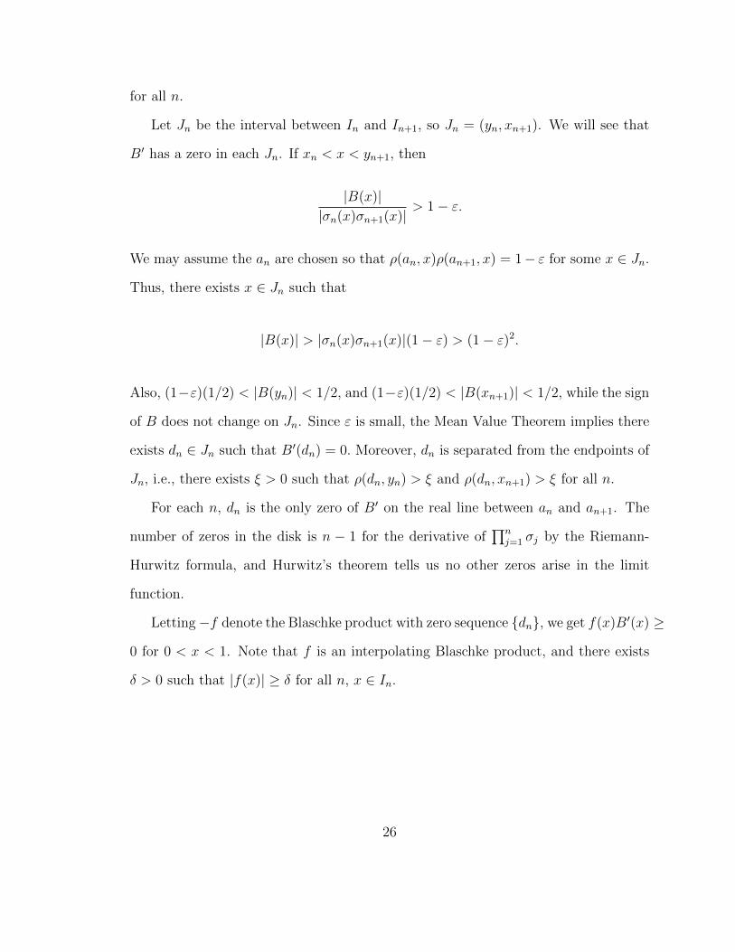
Let Jn be the interval between In and In+1, so Jn = (yn, xn+1). We will see that

B′ has a zero in each Jn. If xn < x < yn+1, then

|B(x)||σn(x)σn+1(x)|

> 1− ε.

We may assume the an are chosen so that ρ(an, x)ρ(an+1, x) = 1− ε for some x ∈ Jn.

Thus, there exists x ∈ Jn such that

|B(x)| > |σn(x)σn+1(x)|(1− ε) > (1− ε)2.

Also, (1−ε)(1/2) < |B(yn)| < 1/2, and (1−ε)(1/2) < |B(xn+1)| < 1/2, while the sign

of B does not change on Jn. Since ε is small, the Mean Value Theorem implies there

exists dn ∈ Jn such that B′(dn) = 0. Moreover, dn is separated from the endpoints of

Jn, i.e., there exists ξ > 0 such that ρ(dn, yn) > ξ and ρ(dn, xn+1) > ξ for all n.

For each n, dn is the only zero of B′ on the real line between an and an+1. The

number of zeros in the disk is n − 1 for the derivative of∏n

j=1 σj by the Riemann-

Hurwitz formula, and Hurwitz’s theorem tells us no other zeros arise in the limit

function.

Letting−f denote the Blaschke product with zero sequence {dn}, we get f(x)B′(x) ≥

0 for 0 < x < 1. Note that f is an interpolating Blaschke product, and there exists

δ > 0 such that |f(x)| ≥ δ for all n, x ∈ In.

26

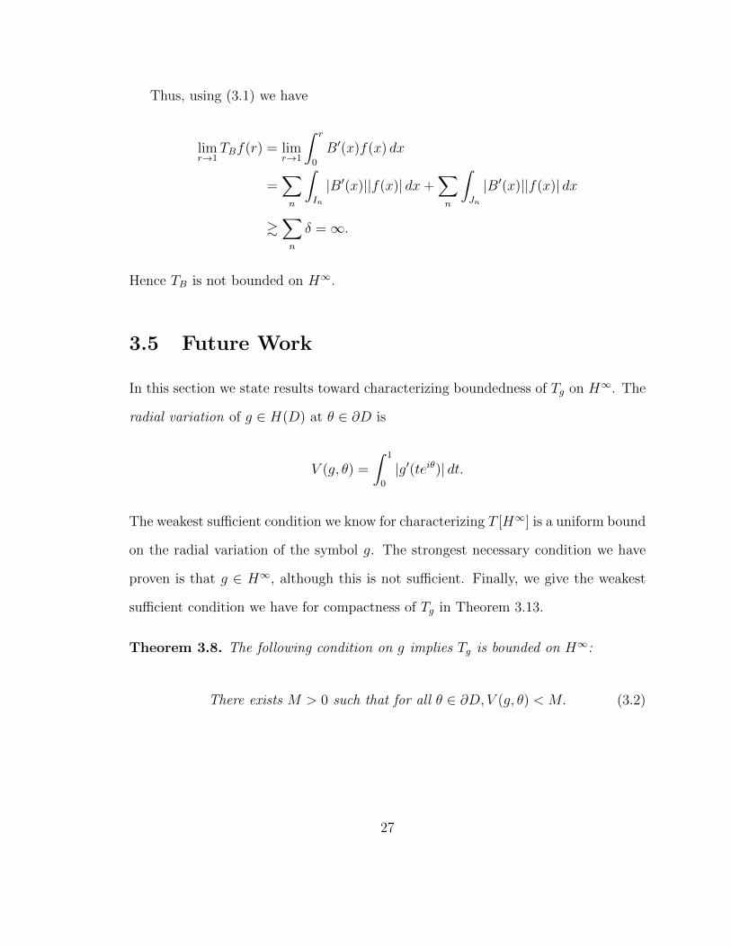
Thus, using (3.1) we have

limr→1

TBf(r) = limr→1

∫ r

0

B′(x)f(x) dx

=∑n

∫In

|B′(x)||f(x)| dx+∑n

∫Jn

|B′(x)||f(x)| dx

&∑n

δ =∞.

Hence TB is not bounded on H∞.

3.5 Future Work

In this section we state results toward characterizing boundedness of Tg on H∞. The

radial variation of g ∈ H(D) at θ ∈ ∂D is

V (g, θ) =

∫ 1

0

|g′(teiθ)| dt.

The weakest sufficient condition we know for characterizing T [H∞] is a uniform bound

on the radial variation of the symbol g. The strongest necessary condition we have

proven is that g ∈ H∞, although this is not sufficient. Finally, we give the weakest

sufficient condition we have for compactness of Tg in Theorem 3.13.

Theorem 3.8. The following condition on g implies Tg is bounded on H∞:

There exists M > 0 such that for all θ ∈ ∂D, V (g, θ) < M. (3.2)

27

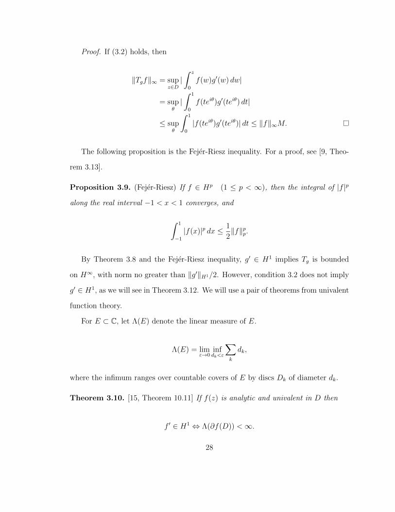
Proof. If (3.2) holds, then

‖Tgf‖∞ = supz∈D|∫ z

0

f(w)g′(w) dw|

= supθ|∫ 1

0

f(teiθ)g′(teiθ) dt|

≤ supθ

∫ 1

0

|f(teiθ)g′(teiθ)| dt ≤ ‖f‖∞M.

The following proposition is the Fejer-Riesz inequality. For a proof, see [9, Theo-

rem 3.13].

Proposition 3.9. (Fejer-Riesz) If f ∈ Hp (1 ≤ p < ∞), then the integral of |f |p

along the real interval −1 < x < 1 converges, and

∫ 1

−1|f(x)|p dx ≤ 1

2‖f‖pp.

By Theorem 3.8 and the Fejer-Riesz inequality, g′ ∈ H1 implies Tg is bounded

on H∞, with norm no greater than ‖g′‖H1/2. However, condition 3.2 does not imply

g′ ∈ H1, as we will see in Theorem 3.12. We will use a pair of theorems from univalent

function theory.

For E ⊂ C, let Λ(E) denote the linear measure of E.

Λ(E) = limε→0

infdk<ε

∑k

dk,

where the infimum ranges over countable covers of E by discs Dk of diameter dk.

Theorem 3.10. [15, Theorem 10.11] If f(z) is analytic and univalent in D then

f ′ ∈ H1 ⇔ Λ(∂f(D)) <∞.

28

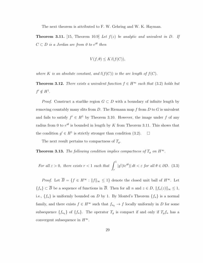
The next theorem is attributed to F. W. Gehring and W. K. Hayman.

Theorem 3.11. [15, Theorem 10.9] Let f(z) be analytic and univalent in D. If

C ⊂ D is a Jordan arc from 0 to eiθ then

V (f, θ) ≤ K l(f(C)),

where K is an absolute constant, and l(f(C)) is the arc length of f(C).

Theorem 3.12. There exists a univalent function f ∈ H∞ such that (3.2) holds but

f ′ /∈ H1.

Proof. Construct a starlike region G ⊂ D with a boundary of infinite length by

removing countably many slits from D. The Riemann map f from D to G is univalent

and fails to satisfy f ′ ∈ H1 by Theorem 3.10. However, the image under f of any

radius from 0 to eiθ is bounded in length by K from Theorem 3.11. This shows that

the condition g′ ∈ H1 is strictly stronger than condition (3.2).

The next result pertains to compactness of Tg.

Theorem 3.13. The following condition implies compactness of Tg on H∞.

For all ε > 0, there exists r < 1 such that

∫ 1

r

|g′(teiθ)| dt < ε for all θ ∈ ∂D. (3.3)

Proof. Let B = {f ∈ H∞ : ‖f‖∞ ≤ 1} denote the closed unit ball of H∞. Let

{fn} ⊂ B be a sequence of functions in B. Then for all n and z ∈ D, ‖fn(z)‖∞ ≤ 1,

i.e., {fn} is uniformly bounded on D by 1. By Montel’s Theorem {fn} is a normal

family, and there exists f ∈ H∞ such that fnk → f locally uniformly in D for some

subsequence {fnk} of {fn}. The operator Tg is compact if and only if Tgfn has a

convergent subsequence in H∞.

29

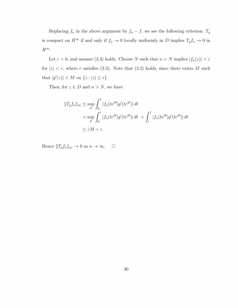
Replacing fn in the above argument by fn − f , we see the following criterion: Tg

is compact on H∞ if and only if fn → 0 locally uniformly in D implies Tgfn → 0 in

H∞.

Let ε > 0, and assume (3.3) holds. Choose N such that n > N implies |fn(z)| < ε

for |z| < r, where r satisfies (3.3). Note that (3.2) holds, since there exists M such

that |g′(z)| < M on {z : |z| ≤ r}.

Then, for z ∈ D and n > N , we have

‖Tgfn‖∞ ≤ supθ

∫ 1

0

|fn(teiθ)g′(teiθ)| dt

= supθ

∫ r

0

|fn(teiθ)g′(teiθ)| dt +

∫ 1

r

|fn(teiθ)g′(teiθ)| dt

≤ εM + ε.

Hence ‖Tgfn‖∞ → 0 as n→∞.

30

Chapter 4

Results on Closed Range Operators

4.1 When Tg Is Bounded Below

We will show that Tg is never bounded below onH2, B, or BMOA. The sequence {zn}

demonstrates the result in each space, since the functions zn have norm comparable

to 1, independent of n (Lemma 2.4).

Theorem 4.1. Tg is never bounded below on H2, B, or BMOA.

Proof. Let fn(z) = zn. For H2, the Littlewood-Paley identity gives us

limn→∞

‖Tgfn‖22 ∼ limn→∞

∫D

|zn|2|g′(z)|2(1− |z|2) dA(z).

We assume Tg is bounded, so g ∈ BMOA by the result of Aleman and Siskakis [4].

Thus µg is a Carleson measure, allowing us to bring the limit inside the integral by

the Dominated Convergence Theorem in the following:

limn→∞

‖Tgfn‖22 =

∫D

limn→∞

|zn|2|g′(z)|2(1− |z|2) dA(z) = 0.

31

Since ‖fn‖2 = 1 for all n, we have shown Tg is not bounded below.

If Tg is bounded on B, then, by Theorem 2.2, |g′(z)|(1−|z|) = O(1/ log(1/(1−|z|)))

as |z| → 1. Thus,

‖Tgfn‖B = supz∈D|zn||g′(z)|(1− |z|) . sup

0≤r<1rn

1

log(2/(1− r)).

Given ε > 0, there exists δ < 1 such that 1/ log(2/(1 − r)) < ε for δ < r < 1. For

large n and 0 < r < δ, we have rn < ε. Thus, limn→∞ ‖Tgfn‖B = 0, and Lemma 2.4

implies Tg is not bounded below on B.

Siskakis and Zhao [17] proved that if Tg is bounded on BMOA then g ∈ LMOA.

Using the relationship between BMOA and Carleson measures for H2, we have

limn→∞

‖Tgfn‖2∗ ∼ limn→∞

supI

1

|I|

∫S(I)

|zn|2|g′(z)|2(1− |z|2) dA(z).

Let I be an arc in ∂D, and let ε > 0. Since g ∈ VMOA, there exists δ > 0 such that

1

|J |

∫S(J)

|g′(z)|2(1− |z|2) dA(z) < ε whenever |J | < δ.

If |I| > δ, divide I into K disjoint intervals of length approximately δ, so

I = ∪Ki=1Ji, δ/2 < |Ji| < δ for all i, and δK ∼ |I|.

Let Sδ(I) = S(I)− ∪iS(Ji). For large n we have (1− δ/2)2n ≤ ε|I|, and to estimate

32

the integral over Sδ(I) we use the fact that µg is a Carleson measure. Thus,

1

|I|

∫S(I)

|zn|2|g′(z)|2(1− |z|2) dA(z) =1

|I|

∫Sδ(I)

|zn|2|g′(z)|2(1− |z|2) dA(z)

+1

|I|

K∑i=1

∫S(Ji)

|zn|2|g′(z)|2(1− |z|2) dA(z)

≤ 1

|I|(1− δ/2)2nC‖g‖2∗ +

1

|I|Kδε . ε.

Hence limn→∞ ‖Tgfn‖∗ = 0 and Tg is not bounded below on BMOA.

In contrast to Theorem 4.1, Tg can be bounded below on weighted Bergman

spaces. We state the result here, but the key is Proposition 4.3, proved afterward.

For a measurable set G ⊂ D, |G| denotes the Lebesque area measure of G.

Theorem 4.2. Let 1 ≤ p < ∞, α > −1. Tg is bounded below on Apα if and only if

there exist c > 0 and δ > 0 such that, for all I ⊂ ∂D,

|{z ∈ D : |g′(z)|(1− |z|2) > c} ∩ S(I)| > δ|I|2.

Proof. We must assume Tg is bounded on Apα. By Theorem 3.2, g ∈ B. Tg is

bounded below on Apα if and only if

‖Tgf‖pApα ∼∫D

|f(z)|p|g′(z)|p(1− |z|2)α+p dA(z) & ‖f‖pApα. (4.1)

By Proposition 4.3, (4.1) holds if and only if there exist c > 0 and δ > 0 such that

|{z ∈ D : |g′(z)|p(1− |z|2)p > c} ∩ S(I)| > δ|I|2 (4.2)

for all arcs I ⊆ ∂D. If (4.2) holds for some p ≥ 1, it holds for 1 ≤ p < ∞, with an

33

adjustment of the constant c.

The proof of [16, Proposition 5.4] shows this result is nonvacuous. Ramey and

Ullrich construct a Bloch function g such that |g′(z)|(1− |z|) > c0 if 1− q−(k+1/2) ≤

|z| ≤ 1−q−(k+1), for some c0 > 0, q some large positive integer, and k = 1, 2, .... Given

a Carleson square S(I), let kI be the least positive integer such that q−kI+1/2 ≤ |I|.

The annulus E = {z : 1− q−(kI+1/2) ≤ |z| ≤ 1− q−(kI+1)} intersects S(I), and

|E ∩ S(I)| ∼ |I|((1− q−(kI+1))− (1− q−(kI+1/2))) = |I|q1/2 − 1

qkI+1≥ (q1/2 − 1)

q3/2|I|2.

Setting c = c0 and δ ∼ 1/q show Theorem 4.2 holds for this example of g, and Tg is

bounded below on Apα.

4.2 When Sg Is Bounded Below

The operator Sg can clearly be bounded below, since g(z) = 1 gives the identity

operator. A result due to Daniel Luecking (see [7, Theorem 3.34]) leads to a charac-

terization of functions for which Sg is bounded below on H20 := H2/C and Apα/C. We

state a reformulation useful to our purposes here.

Proposition 4.3. (Luecking) Let τ be a bounded, nonnegative, measurable function

on D. Let Gc = {z ∈ D : τ(z) > c}, 1 ≤ p < ∞, and α > −1. There exists C > 0

such that the inequality

∫D

|f(z)|pτ(z)(1− |z|)α dA(z) ≥ C

∫D

|f(z)|p(1− |z|)α dA(z)

holds if and only if there exist δ > 0 and c > 0 such that |Gc ∩S(I)| ≥ δ|I|2 for every

interval I ⊂ ∂D.

34

The proof is omitted. Using the Littlewood-Paley identity we get the following:

Corollary 4.4. Sg is bounded below on H20 if and only if there exist c > 0 and δ > 0

such that |Gc ∩ S(I)| ≥ δ|I|2 for all I ⊂ ∂D, where Gc = {z ∈ D : |g(z)| > c} .

We use Corollary 4.4 to exhibit an example when Sg is not bounded below on H20 .

If g(z) is the singular inner function exp( z+1z−1), Sg is not bounded below on H2

0 . To

see this, fix c ∈ (0, 1). Gc is the complement in D of a horodisk, a disk tangent to

the unit circle, with radius r = log c+12(log c−1) and center 1 − r. Choosing a sequence of

intervals In ⊂ ∂D such that 1 is the center of In and |In| → 0 as n→∞, we see

|Gc ∩ S(In)||In|2

→ 0 as n→∞,

meaning Sg is not bounded below on H20 .

We compare Mg on H2 to Sg on H20 . Mg is bounded below on H2 if and only

if the radial limit function of g ∈ H∞ is essentially bounded away from 0 on ∂D (a

special case of weighted composition operators; see [12]). Theorem 4.6 will show this

is weaker than the condition for Sg to be bounded below on H20 . The example above

of a singular inner function then shows it is strictly weaker. To prove Theorem 4.6

we use a lemma which allows us to estimate an analytic function inside the disk by

its values on the boundary.

For any arc I ⊆ ∂D and 0 < r < 2π/|I|, rI will denote the arc with the same

center as I and length r|I|. We define the upper Carleson rectangle by

Sε(I) = {reit : 1− |I| < r < (1− ε|I|), eit ∈ I}, and S+(I) = S1/2(I).

Lemma 4.5. Given ε, 0 < ε < 1, and a point eiθ such that |g∗(eiθ)| < ε, there exists

35

an arc I ⊂ ∂D such that |g(z)| < ε for z ∈ Sε(I).

Proof. We can choose α close enough to 1 so that Sε(I) ⊂ Γα(eiθ) for all I centered

at eiθ with, say, |I| < 1/4. If |g∗(eiθ)| < ε, there exists δ > 0 such that

z ∈ Γα(eiθ) and |z − eiθ| < δ implies |g(z)| < ε.

Choosing I such that S(I) is contained in a δ-neighborhood of eiθ finishes the proof.

Theorem 4.6. If Sg is bounded below on H20 , then Mg is bounded below on H2.

Proof. Assume Mg is not bounded below on H2. Let ε > 0. The radial limit func-

tion of g equals g∗ almost everywhere, so there exists a point eiθ such that |g∗(eiθ)| < ε.

By Lemma 4.5, there exists S(I) such that |{z : |g(z)| ≥ ε} ∩ S(I)| ≤ ε|I|. Since ε

was arbitrary, this violates the condition in Corollary 4.4.

4.2.1 Sg on the Bloch Space

We now characterize the symbols g which make Sg bounded below on the Bloch

space. It turns out to be a common condition appearing in a few different forms in

the literature. The condition appears in characterizing Mg on A20 in McDonald and

Sundberg [14]. Our main result is equivalence of (i)-(iii) in Theorem 4.7, and we give

references with brief explanations for (iv)-(vi).

An infinite Blaschke product is a function on D of the form

B(z) = zm∏n

−an|an|

z − an1− anz

,

36

where m is a nonnegative integer, 0 6= an ∈ D for n = 1, 2, 3, ..., and

∑n

(1− |an|) <∞.

A sequence {an} is an interpolating sequence if, given {wn} ∈ `∞, there exists f ∈ H∞

such that

f(an) = wn for all n.

An interpolating sequence {an} must satisfy

ρ(aj, ak) > δ for all j 6= k and some δ > 0, (4.3)

where ρ(aj, ak) = |aj − ak|/|1− akaj| denotes the pseudohyperbolic distance between

ak and aj. A well-known result of Carleson is that the sequence {an} is interpolating

if and only if (4.3) holds and the measure∑

(1 − |an|)δan is a Carleson measure for

H1 (see [11, Theorem VII.1.1]).

Letting {an} be the sequence of zeros of B (an = 0 is possible), the Blaschke

product B is interpolating if {an} is an interpolating sequence.

For the pseudohyperbolic disk of radius d > 0 and center w ∈ D, we use the

notation

D(w, d) = {z ∈ D : ρ(z, w) < d}.

Theorem 4.7. The following are equivalent for g ∈ H∞:

(i) g = BF for a finite product B of interpolating Blaschke products and F such

that F and 1/F ∈ H∞.

(ii) Sg is bounded below on B/C.

37

(iii) There exist r < 1 and η > 0 such that for all a ∈ D,

supz∈D(a,r)

|g(z)| > η.

(iv) Sg is bounded below on H20 .

(v) Mg is bounded below on Apα for α > −1.

(vi) Sg is bounded below on Apα/C for α > −1.

Proof. (i) ⇒ (ii): Note that for any g1, g2 ∈ H(D),

Sg1g2 = Sg1Sg2 . (4.4)

If Sg is bounded on B, then g ∈ H∞ by Corollary 2.3. If F and 1/F ∈ H∞, then

‖SFf‖ = supz∈D|F (z)||f ′(z)|(1− |z|2) ≥ (1/‖1/F‖∞)‖f‖B.

Hence SF is bounded below.

The product of two interpolating Blaschke products is not necessarily an interpo-

lating Blaschke product. For example, B2 fails to satisfy (4.3) for any interpolating

Blaschke product B. However, by virtue of (4.4), we may assume B is a single inter-

polating Blaschke product without loss of generality. Let {wn} be the zero sequence

of B, so

B(z) =∏n

wn|wn|

wn − z1− wnz

.

Let Bj be B without its jth zero, i.e., Bj(z) =1−wjzwj−z B(z). Since B is interpolating,

there exist δ > 0 and r > 0 such that, for all j, |Bj(z)| > δ whenever z ∈ D(wj, r).

In particular, the sequence {wn} is separated, so shrinking r if necessary, we may

38

assume

infj 6=k

ρ(wk, wj) > 2r.

We compare ‖f‖ to ‖SBf‖ = supz∈D |B(z)||f ′(z)|(1− |z|2). Let a ∈ D be a point

where the supremum defining the norm of f is almost achieved, say, |f ′(a)|(1−|a|2) >

‖f‖/2.

Consider the pseudohyperbolic disk D(a, r). Inside D(a, r) there may be at most

one zero of B, or there may not be a zero. If the zero exists call it wk. We examine

three cases depending on the location and existence of wk.

If r/2 ≤ ρ(wk, a) < r, then

|B(a)| = |wk − a||1− wka|

|Bk(a)| > (r/2)δ.

Thus, we would have

‖SBf‖ ≥ |B(a)||f ′(a)|(1− |a|2) > (r/2)δ‖f‖/2,

and Sg would be bounded below.

On the other hand, suppose ρ(wk, a) < r/2. Consider the disk D(wk, r/2), which is

contained inD(a, r). The expression 1−|z|2 is roughly constant on a pseudohyperbolic

disk, i.e.,

supz∈D(a,r)

(1− |z|2) > Cr(1− |a|2) for some Cr > 0.

Cr does not depend on a, and is near 1 for small r. By the maximum principle for

f ′, there exists a point za ∈ ∂D(wk, r/2) where

|f ′(za)|(1− |za|2) > |f ′(a)|Cr(1− |a|2) > Cr‖f‖/2.

39

(Since ρ(wk, a) < r/2 and ρ(za, wk) = r/2, we have ρ(za, a) < r.) This shows that Sg

is bounded below, for

‖SBf‖ ≥ |B(za)||f ′(za)|(1− |za|2)

> ρ(wk, za)|Bk(za)|Cr‖f‖/2

> (r/2)δCr‖f‖/2.

Finally, suppose no such wk exists. Then the function ((a − z)/(1 − az))B(z) is

also an interpolating Blaschke product, and the previous case applies with wk = a.

(ii) ⇒ (iii): Assume (iii) fails. Given ε > 0, choose r near 1 so that 1 − r2 < ε,

and choose a ∈ D such that |g(z)| < ε for all z ∈ D(a, r). Consider the test function

fa(z) = (a− z)/(1− az). By a well-known identity (see [11, p.3]),

(1− |z|2)|f ′a(z)| = 1− (ρ(a, z))2.

Thus fa ∈ B with ‖fa‖ = 1 for all a ∈ D. (The seminorm is 1, but the true norm is

between 1 and 2 for all a.) Since (iii) fails, we have

‖Sgfa‖ = supz∈D|g(z)||f ′a(z)|(1− |z|2)

= max

{sup

z∈D(a,r)

|g(z)||f ′a(z)|(1− |z|2), supz∈D\D(a,r)

|g(z)||f ′a(z)|(1− |z|2)}

≤ max

{sup

z∈D(a,r)

|g(z)|‖fa‖, supz∈D\D(a,r)

|g(z)|(1− r2)}

< max{ε, ‖g‖∞ε} ≤ ε(‖g‖∞ + 1)

Since ‖fa‖ = 1 and ε was arbitrary, Sg is not bounded below.

(iii) ⇒ (i): Assuming (iii) holds, we first rule out the possibility that g has a

40

singular inner factor. We factor g = BIgOg where B is a Blaschke product, Ig a

singular inner function, and Og an outer function. Let ν be the measure on ∂D

determining Ig, so

Ig(z) = exp

(−∫

eiθ + z

eiθ − zdν(θ)

).

Let ε > 0. For any α > 1 and for ν-almost all θ, there exists δ > 0 such that

z ∈ Γα(eiθ) and |z − eiθ| < δ implies |Ig(z)| < ε (4.5)

(see [11, Theorem II.6.2]). The constant δ may depend on θ and α, but for nontrivial

ν there exists some θ for which (4.5) holds. Given r < 1, choose α < 1 such that,

for every a near eiθ on the ray from 0 to eiθ, the pseudohyperbolic disk D(a, r) is

contained in Γα(eiθ). The disk D(a, r) is a euclidean disk whose euclidean radius is

comparable to 1− a. For a close enough to eiθ,

z ∈ D(a, r) implies |z − eiθ| < δ.

Hence supz∈D(a,r) |g(z)| < ε‖g‖. This violates (iii), so ν must be trivial, and Ig ≡ 1.

A similar argument handles the outer function Og. If for all ε > 0 there exists

eit such that |O∗g(eit)| < ε, we apply Lemma 4.5. The upper Carleson square in

Lemma 4.5 contains some pseudohyperbolic disk that violates (iii), so O∗g is essentially

bounded away from 0. There exists η > 0, such that |O∗g(eit)| ≥ η almost everywhere.

Note 1/Og ∈ H∞, since for all z ∈ D,

log |Og(z)| = 1

2π

∫ 2π

0

log |O∗g(eit)|1− |z|2

|eit − z|2dt ≥ log η.

41

We have reduced the symbol to a function g = BF , where F, 1/F ∈ H∞ and B

is a Blaschke product, say with zero sequence {wn}. We will show that the measure

µB =∑

(1 − |wn|2)δwn is a Carleson measure, implying B is a finite product of

interpolating Blaschke products (see, e.g., [14, Lemma 21]). Let r < 1 and η > 0

be as in (iii), so supz∈D(a,r) |B(z)| > η for all a. Given any arc I ⊆ ∂D, we may

choose aI and zI such that zI ∈ D(aI , r) ⊆ S(I) and |B(zI)| > η. We may also

ensure (1 − |zI |) ∼ |I| as I varies. Note that µB(S(I)) =∑

(1 − |wnk |2), for the

subsequence {wnk} = {wn} ∩ S(I). Assume without loss of generality that |I| < 1/2,

so |wnk | > 1/2 for all k. This ensures |1− wnkzI | ∼ |I|. Thus we have

1

|I|∑k

(1− |wnk |2) ∼∑k

(1− |zI |2)(1− |wnk |2)|1− wnkzI |2

=∑k

1− (ρ(zI , wnk))2

< 2∑n

1− ρ(zI , wn)

≤ −∑n

log ρ(zI , wn)

= − log∏n

|wn − zI ||1− wnzI |

= − log |B(z)| ≤ − log η.

This shows µB is a Carleson measure, hence (iii) ⇒ (i).

Bourdon shows in [6, Theorem 2.3, Corollary 2.5] that (i) is equivalent to the

reverse Carleson condition in Corollary 4.4 above, hence (i) ⇔ (iv). This reverse

Carleson condition also characterizes boundedness below of Mg on weighted Bergman

spaces by Proposition 4.3. Thus (iv)⇔ (v). The equivalence of (v) and (vi) is evident

from the differentiation isomorphism (2.4).

42

4.2.2 Concluding Remarks

We suspect the results about H2 can be extended to all Hp, 1 ≤ p <∞, but without

the Littlewood-Paley identity the proof will be more difficult. Generalizing the results

on the Bloch space to the α-Bloch spaces can be done with adjusted test functions

as in [20]. Finally, we have partial results concerning Sg being bounded below on

BMOA, but have not completed proving a characterization like the one in Theorem

4.7.

43

Bibliography

[1] Aleman, Alexandru, Some open problems on a class of integral operators on

spaces of analytic functions. Topics in complex analysis and operator theory,

139140, Univ. Mlaga, Mlaga, 2007.

[2] Aleman, Alexandru; Cima, Joseph A., An integral operator on Hp and Hardy’s

inequality. J. Anal. Math. 85 (2001), 157–176.

[3] Aleman, Alexandru; Siskakis, Aristomenis G. An integral operator on Hp. Com-

plex Variables Theory Appl. 28 (1995), no. 2, 149–158.

[4] Aleman, Alexandru; Siskakis, Aristomenis G., Integration operators on

Bergman spaces. Indiana Univ. Math. J. 46 (1997), no. 2, 337–356.

[5] Arazy, Jonathan, Multipliers of Bloch Functions. University of Haifa Publica-

tion Series 54 (1982).

[6] Bourdon, Paul S., Similarity of parts to the whole for certain multiplication

operators. Proc. Amer. Math. Soc. 99 (1987), no. 3, 563–567.

[7] Cowen, Carl; MacCluer, Barbara, Composition Operators on Spaces of Analytic

Functions. CRC Press, New York, 1995.

44

[8] Dostanic, Milutin R., Integration operators on Bergman spaces with exponential

weight. Rev. Mat. Iberoam. 23 (2007), no. 2, 421–436.

[9] Duren, P. L., Theory of Hp spaces. Dover, New York, 2000.

[10] Duren, P. L.; Romberg, B. W.; Shields, A. L., Linear functionals on Hp spaces

with 0 < p < 1. J. Reine Angew. Math. 238 (1969), 32-60.

[11] Garnett, John B., Bounded Analytic Functions. Revised First Edition. Springer,

New York, 2007.

[12] Kumar, Romesh; Partington, Jonathan R., Weighted composition operators on

Hardy and Bergman spaces. Recent advances in operator theory, operator alge-

bras, and their applications, 157–167, Oper. Theory Adv. Appl., 153, Birkhuser,

Basel, 2005.

[13] Lv, Xiao-fen, Extended Cesaro operator between Bloch-type spaces. Chinese

Quart. J. Math. 24 (2009), no. 1, 1019.

[14] McDonald, G.; Sundberg, C., Toeplitz operators on the disc. Indiana Univ.

Math. J. 28 (1979), no. 4, 595–611.

[15] Pommerenke, Christian, Univalent functions. Studia Mathemat-

ica/Mathematische Lehrbucher, Band XXV. Vandenhoeck & Ruprecht,

Gottingen, 1975.

[16] Ramey, Wade; Ullrich, David, Bounded mean oscillation of Bloch pull-backs.

Math. Ann. 291 (1991), no. 4, 591–606.

45

[17] Siskakis, Aristomenis G.; Zhao, Ruhan, A Volterra type operator on spaces of

analytic functions. Function spaces (Edwardsville, IL, 1998), 299–311, Con-

temp. Math., 232, Amer. Math. Soc., Providence, RI, 1999.

[18] Stegenga, David A., Bounded Toeplitz operators on H1 and applications of the

duality between H1 and the functions of bounded mean oscillation. Amer. J.

Math. 98 (1976), no. 3, 573–589.

[19] Stegenga, David A., Multipliers of the Dirichlet space. Illinois J. Math. 24

(1980), no. 1, 113–139.

[20] Zhang, M.; Chen, H., Weighted composition operators of H∞ into α-Bloch

spaces on the unit ball. Acta Math. Sin. (Engl. Ser.) 25 (2009), no. 2, 265–

278.

[21] Zhu, Kehe, Operator theory in function spaces. Second edition. Mathematical

Surveys and Monographs, 138. American Mathematical Society, Providence,

RI, 2007.

46