MULTIRATE SIGNAL PROCESSING - NYU Tandon …eeweb.poly.edu/iselesni/EL713/zoom/mrate.pdf · MULTIRATE SIGNAL PROCESSING 1.APPLICATIONS ... is de ned by the relation y(n) = ... 6;0;:::g:

MULTIRATE SIGNAL PROCESSING

1. APPLICATIONS

2. THE UP-SAMPLER

3. THE DOWN-SAMPLER

4. RATE-CHANGING

5. INTERPOLATION

6. HALF-BAND FILTERS

7. NYQUIST FILTERS

8. THE NOBLE IDENTITIES

9. POLYPHASE DECOMPOSITION

10. EFFICIENT IMPLEMENTATION

11. POLYNOMIALS AND MULTIRATE FILTERING

12. INTERPOLATION OF POLYNOMIALS

I. Selesnick EL 713 Lecture Notes 1

APPLICATIONS

1. Used in A/D and D/A converters.

2. Used to change the rate of a signal. When two devices that op-

erate at different rates are to be interconnected, it is necessary

to use a rate changer between them.

3. Interpolation.

4. Some efficient implementations of single rate filters are based

on multirate methods.

5. Filter banks and wavelet transforms depend on multirate meth-

ods.


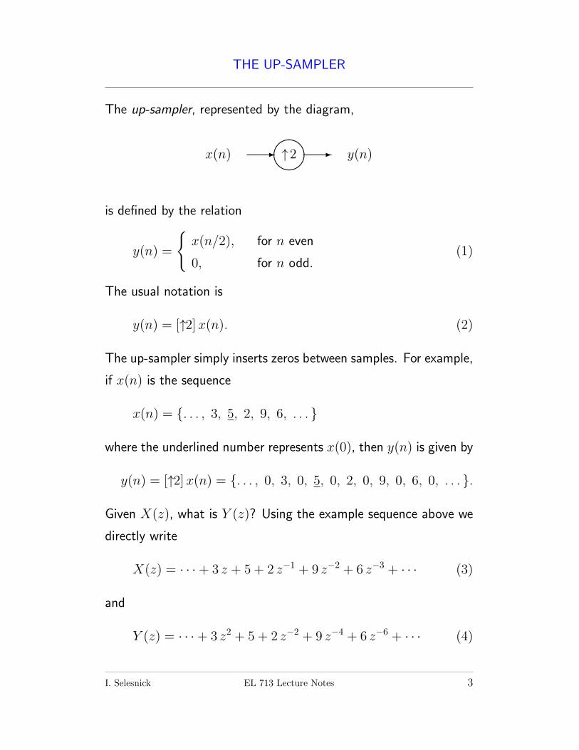
THE UP-SAMPLER

The up-sampler, represented by the diagram,

x(n) -��↑2 - y(n)

is defined by the relation

y(n) =

{x(n/2), for n even

0, for n odd.(1)

The usual notation is

y(n) = [↑2]x(n). (2)

The up-sampler simply inserts zeros between samples. For example,

if x(n) is the sequence

x(n) = {. . . , 3, 5, 2, 9, 6, . . . }

where the underlined number represents x(0), then y(n) is given by

y(n) = [↑2]x(n) = {. . . , 0, 3, 0, 5, 0, 2, 0, 9, 0, 6, 0, . . . }.

Given X(z), what is Y (z)? Using the example sequence above we

directly write

X(z) = · · ·+ 3 z + 5 + 2 z−1 + 9 z−2 + 6 z−3 + · · · (3)

and

Y (z) = · · ·+ 3 z2 + 5 + 2 z−2 + 9 z−4 + 6 z−6 + · · · (4)


It is clear that

Y (z) = Z {[↑2]x(n)} = X(z2). (5)

We can also derive this using the definition:

Y (z) =∑n

y(n) z−n (6)

=∑

n evenx(n/2) z−n (7)

=∑n

x(n) z−2n (8)

= X(z2). (9)

How does up-sampling affect the Fourier transform of a signal?

The discrete-time Fourier transform of y(n) is given by

Y (ejω) = X(z2)∣∣z=ejω

(10)

= X((ejω)2) (11)

so we have

Y (ejω) = X(ej2ω). (12)

Or using the notation Y f(ω) = Y (ejω), Xf(ω) = X(ejω), we have

Y f(ω) = DTFT {[↑2]x(n)} = Xf(2ω). (13)

When sketching the Fourier transform of an up-sampled signal, it is

easy to make a mistake. When the Fourier transform is as shown in

the following figure, it is easy to incorrectly think that the Fourier

transform of y(n) is given by the second figure. This is not correct,

because the Fourier transform is 2π-periodic. Even though it is

usually graphed in the range −π ≤ ω ≤ π or 0 ≤ ω ≤ π, outside


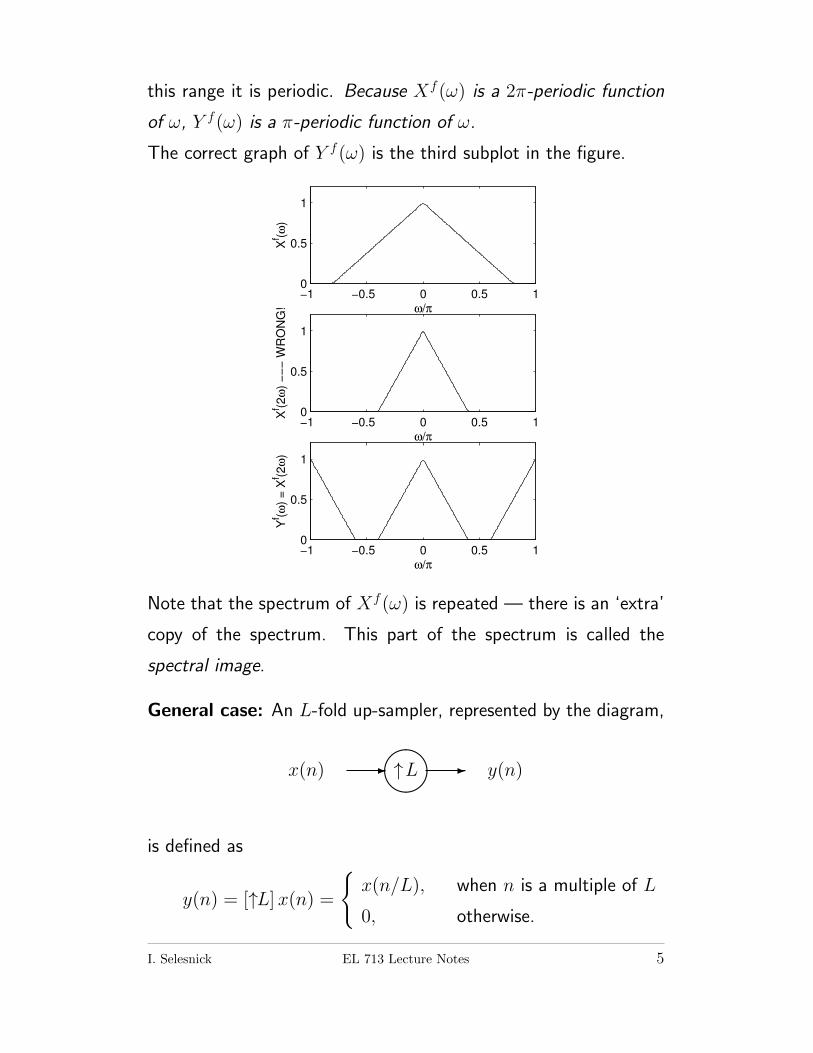
this range it is periodic. Because Xf(ω) is a 2π-periodic function

of ω, Y f(ω) is a π-periodic function of ω.

The correct graph of Y f(ω) is the third subplot in the figure.

−1 −0.5 0 0.5 10

0.5

1

Xf (ω

)

ω/π

−1 −0.5 0 0.5 10

0.5

1

Yf (ω

) =

Xf (2

ω)

ω/π

−1 −0.5 0 0.5 10

0.5

1

Xf (2

ω)

−−

− W

RO

NG

!

ω/π

Note that the spectrum of Xf(ω) is repeated — there is an ‘extra’

copy of the spectrum. This part of the spectrum is called the

spectral image.

General case: An L-fold up-sampler, represented by the diagram,

x(n) -��↑L - y(n)

is defined as

y(n) = [↑L]x(n) =

{x(n/L), when n is a multiple of L

0, otherwise.


(14)

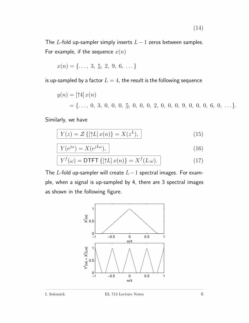
The L-fold up-sampler simply inserts L− 1 zeros between samples.

For example, if the sequence x(n)

x(n) = {. . . , 3, 5, 2, 9, 6, . . . }

is up-sampled by a factor L = 4, the result is the following sequence

y(n) = [↑4]x(n)

= {. . . , 0, 3, 0, 0, 0, 5, 0, 0, 0, 2, 0, 0, 0, 9, 0, 0, 0, 6, 0, . . . }.

Similarly, we have

Y (z) = Z {[↑L]x(n)} = X(zL), (15)

Y (ejω) = X(ejLω), (16)

Y f(ω) = DTFT {[↑L]x(n)} = Xf(Lω). (17)

The L-fold up-sampler will create L−1 spectral images. For exam-

ple, when a signal is up-sampled by 4, there are 3 spectral images

as shown in the following figure.

−1 −0.5 0 0.5 10

0.5

1

Xf (ω

)

ω/π

−1 −0.5 0 0.5 10

0.5

1

Yf (ω

) =

Xf (L

ω)

ω/π


Remarks

1. No information is lost when a signal is up-sampled.

2. The up-sampler is a linear but not a time-invariant system.

3. The up-sampler introduces spectral images.


THE DOWN-SAMPLER

The down-sampler, represented by the following diagram,

x(n) -��↓2 - y(n)

is defined as

y(n) = x(2n). (18)

The usual notation is

y(n) = [↓2]x(n). (19)

The down-sampler simply keeps every second sample, and discards

the others. For example, if x(n) is the sequence

x(n) = {. . . , 7, 3, 5, 2, 9, 6, 4, . . . }

where the underlined number represents x(0), then y(n) is given by

y(n) = [↓2]x(n) = {. . . , 7, 5, 9, 4, . . . }.

Given X(z), what is Y (z)? This is not as simple as it is for the

up-sampler. Using the example sequence above we directly write

X(z) = · · ·+7 z2+3 z+5+2 z−1+9 z−2+6 z−3+4 z−4+· · · (20)

and

Y (z) = · · ·+ 7 z + 5 + 9 z−1 + 4 z−2 + · · · (21)

How can we express Y (z) in terms of X(z)? Consider the sum of

X(z) and X(−z). Note that X(−z) is given by

X(−z) = · · ·+7 z2−3 z+5−2 z−1+9 z−2−6 z−3+4 z−4+· · · . (22)


The odd terms are negated. Then

X(z)+X(−z) = 2 ·(· · ·+ 7 z2 + 5 + 9 z−2 + 4 z−4 + · · ·

)(23)

or

X(z) +X(−z) = 2 · Y (z2) (24)

or

Y (z) = Z {[↓2]x(n)} = X(z12 ) +X(−z 1

2 )

2(25)

How does down-sampling affect the Fourier transform of a signal?

The discrete-time Fourier transform of y(n) is given by

Y (ejω) =X(z

12 ) +X(−z 1

2 )

2

∣∣∣∣∣z=ejω

(26)

=1

2·(X(ej

ω2 ) +X(−ej

ω2 ))

(27)

=1

2·(X(ej

ω2 ) +X(e−jπ ej

ω2 ))

(28)

=1

2·(X(ej

ω2 ) +X(ej(

ω2−π))

)(29)

=1

2·(Xf(

ω

2) +Xf(

ω − 2π

2)

)(30)

Y f(ω) = DTFT {[↓2]x(n)} = 1

2·(Xf(

ω

2) +Xf(

ω − 2π

2)

)(31)

where we have used the notation Y f(ω) = Y (ejω), Xf(ω) =

X(ejω).

Note that because Xf(ω) is periodic with a period of 2π, the func-

tions Xf(ω2 ) and Xf(ω−2π2 ) are each periodic with a period of 4π.


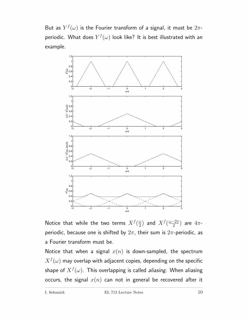
But as Y f(ω) is the Fourier transform of a signal, it must be 2π-

periodic. What does Y f(ω) look like? It is best illustrated with an

example.

−3 −2 −1 0 1 2 30

0.2

0.4

0.6

0.8

1

1.2

Xf (ω

)

ω/π

−3 −2 −1 0 1 2 30

0.2

0.4

0.6

0.8

1

1.2

0.5

* X

f (ω/2

)

ω/π

−3 −2 −1 0 1 2 30

0.2

0.4

0.6

0.8

1

1.2

0.5

* X

f ((ω

−2

π)/

2)

ω/π

−3 −2 −1 0 1 2 30

0.2

0.4

0.6

0.8

1

1.2

Yf (ω

)

ω/π

Notice that while the two terms Xf(ω2 ) and Xf(ω−2π2 ) are 4π-

periodic, because one is shifted by 2π, their sum is 2π-periodic, as

a Fourier transform must be.

Notice that when a signal x(n) is down-sampled, the spectrum

Xf(ω) may overlap with adjacent copies, depending on the specific

shape of Xf(ω). This overlapping is called aliasing. When aliasing

occurs, the signal x(n) can not in general be recovered after it


is down-sampled. In this case, information is lost by the down-

sampling. If the spectrum Xf(ω) were zero for π/2 ≤ |ω| ≤ π,

then no overlapping would occur, and it would be possible to recover

x(n) after it is down-sampled.

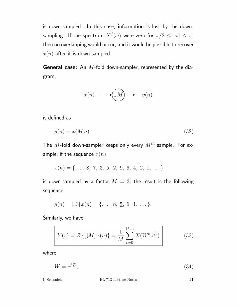
General case: An M -fold down-sampler, represented by the dia-

gram,

x(n) -��↓M - y(n)

is defined as

y(n) = x(M n). (32)

The M -fold down-sampler keeps only every M th sample. For ex-

ample, if the sequence x(n)

x(n) = {. . . , 8, 7, 3, 5, 2, 9, 6, 4, 2, 1, . . . }

is down-sampled by a factor M = 3, the result is the following

sequence

y(n) = [↓3]x(n) = {. . . , 8, 5, 6, 1, . . . }.

Similarly, we have

Y (z) = Z {[↓M ]x(n)} = 1

M

M−1∑k=0

X(W kz1M ) (33)

where

W = ej2πM , (34)


and

Y f(ω) = DTFT {[↓M ]x(n)} = 1

M

M−1∑k=0

Xf

(ω − 2π k

M

). (35)

Remarks

1. In general, information is lost when a signal is down-sampled.

2. The down-sampler is a linear but not a time-invariant system.

3. In general, the down-sampler causes aliasing.


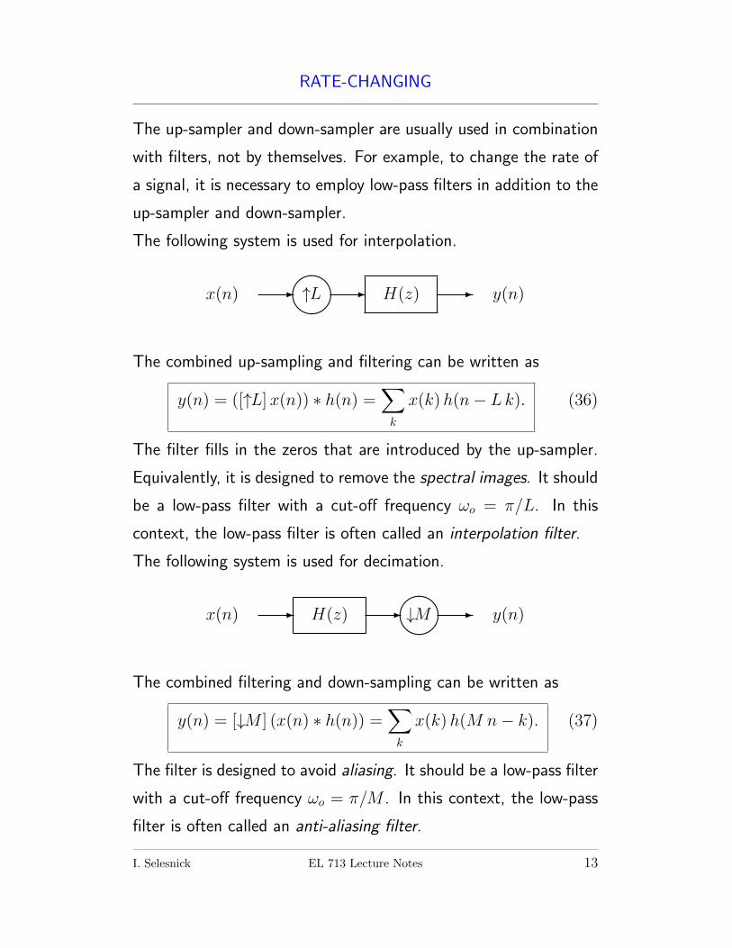
RATE-CHANGING

The up-sampler and down-sampler are usually used in combination

with filters, not by themselves. For example, to change the rate of

a signal, it is necessary to employ low-pass filters in addition to the

up-sampler and down-sampler.

The following system is used for interpolation.

x(n) -��↑L - H(z) - y(n)

The combined up-sampling and filtering can be written as

y(n) = ([↑L]x(n)) ∗ h(n) =∑k

x(k)h(n− Lk). (36)

The filter fills in the zeros that are introduced by the up-sampler.

Equivalently, it is designed to remove the spectral images. It should

be a low-pass filter with a cut-off frequency ωo = π/L. In this

context, the low-pass filter is often called an interpolation filter.

The following system is used for decimation.

x(n) - H(z) -��↓M - y(n)

The combined filtering and down-sampling can be written as

y(n) = [↓M ] (x(n) ∗ h(n)) =∑k

x(k)h(M n− k). (37)

The filter is designed to avoid aliasing. It should be a low-pass filter

with a cut-off frequency ωo = π/M . In this context, the low-pass

filter is often called an anti-aliasing filter.


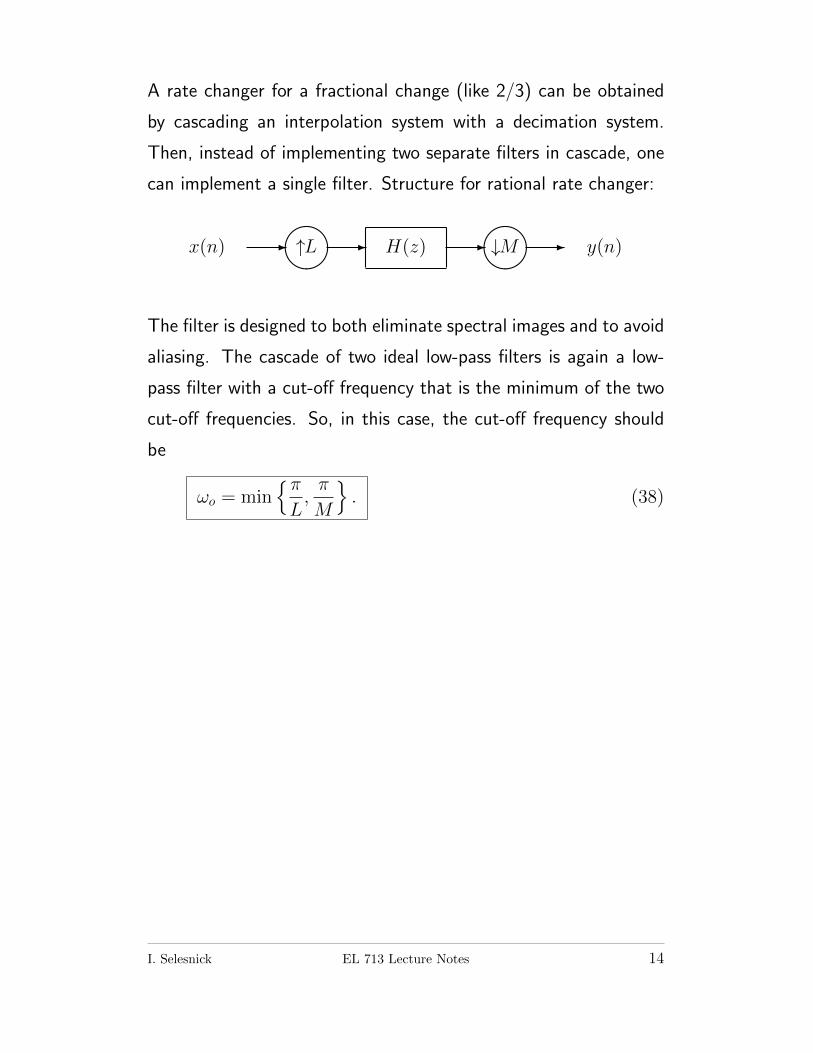
A rate changer for a fractional change (like 2/3) can be obtained

by cascading an interpolation system with a decimation system.

Then, instead of implementing two separate filters in cascade, one

can implement a single filter. Structure for rational rate changer:

x(n) -��↑L - H(z) -��

��↓M - y(n)

The filter is designed to both eliminate spectral images and to avoid

aliasing. The cascade of two ideal low-pass filters is again a low-

pass filter with a cut-off frequency that is the minimum of the two

cut-off frequencies. So, in this case, the cut-off frequency should

be

ωo = min{πL,π

M

}. (38)


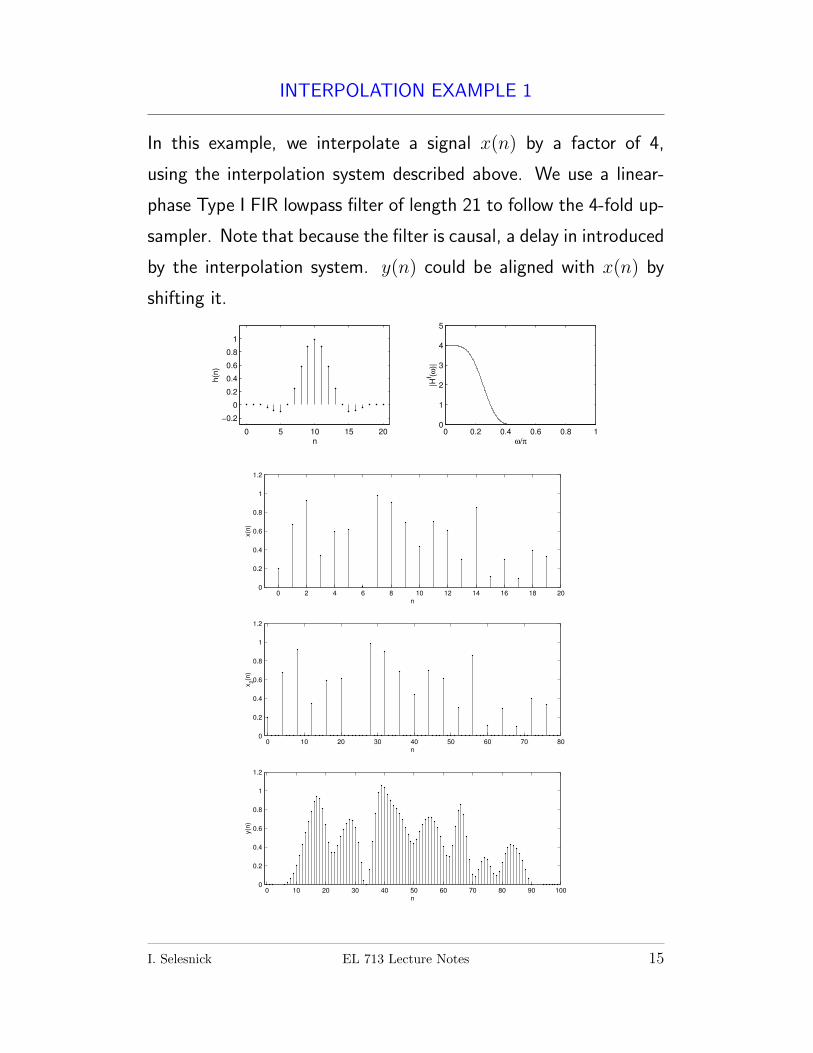
INTERPOLATION EXAMPLE 1

In this example, we interpolate a signal x(n) by a factor of 4,

using the interpolation system described above. We use a linear-

phase Type I FIR lowpass filter of length 21 to follow the 4-fold up-

sampler. Note that because the filter is causal, a delay in introduced

by the interpolation system. y(n) could be aligned with x(n) by

shifting it.

0 5 10 15 20

−0.2

0

0.2

0.4

0.6

0.8

1

n

h(n

)

0 0.2 0.4 0.6 0.8 10

1

2

3

4

5

ω/π|H

f (ω)|

0 2 4 6 8 10 12 14 16 18 200

0.2

0.4

0.6

0.8

1

1.2

n

x(n

)

0 10 20 30 40 50 60 70 800

0.2

0.4

0.6

0.8

1

1.2

n

x2(n

)

0 10 20 30 40 50 60 70 80 90 1000

0.2

0.4

0.6

0.8

1

1.2

n

y(n

)


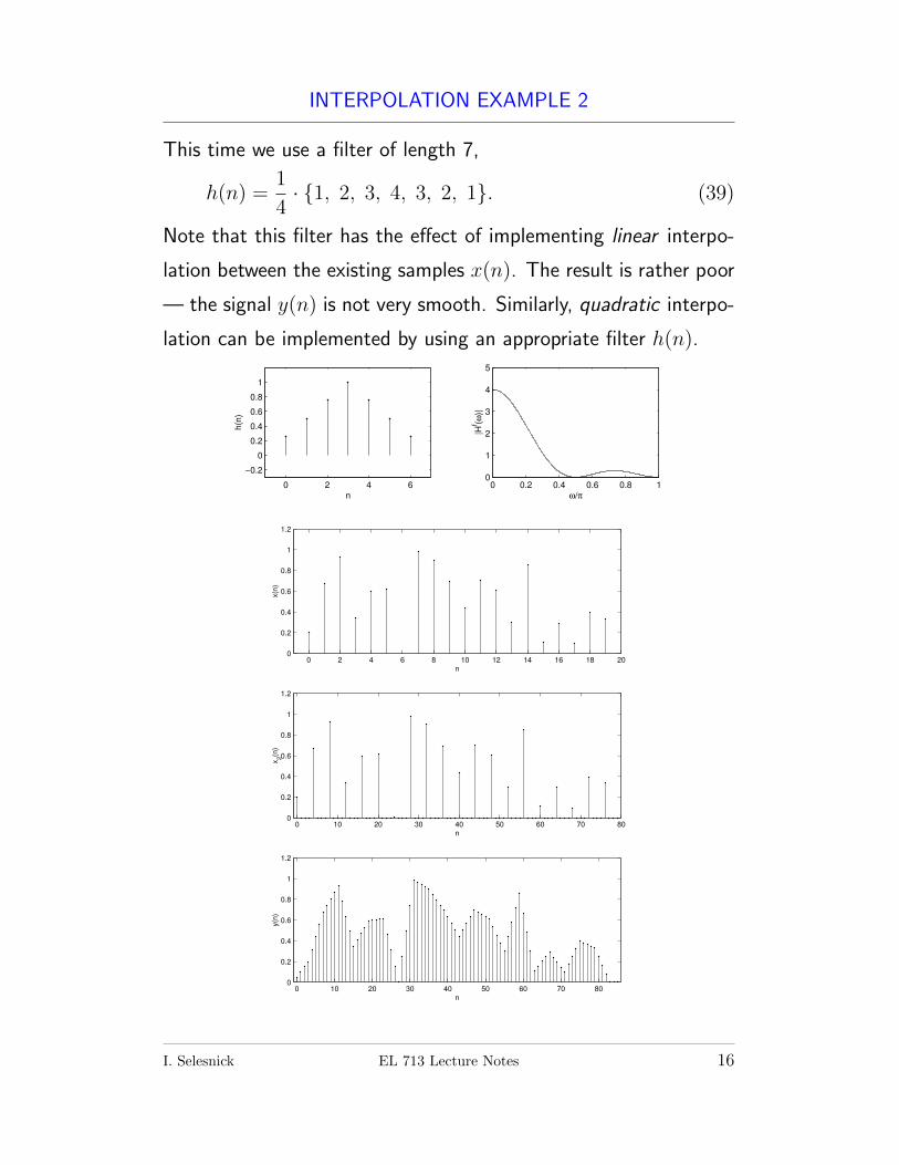
INTERPOLATION EXAMPLE 2

This time we use a filter of length 7,

h(n) =1

4· {1, 2, 3, 4, 3, 2, 1}. (39)

Note that this filter has the effect of implementing linear interpo-

lation between the existing samples x(n). The result is rather poor

— the signal y(n) is not very smooth. Similarly, quadratic interpo-

lation can be implemented by using an appropriate filter h(n).

0 2 4 6

−0.2

0

0.2

0.4

0.6

0.8

1

n

h(n

)

0 0.2 0.4 0.6 0.8 10

1

2

3

4

5

ω/π

|Hf (ω

)|

0 2 4 6 8 10 12 14 16 18 200

0.2

0.4

0.6

0.8

1

1.2

n

x(n

)

0 10 20 30 40 50 60 70 800

0.2

0.4

0.6

0.8

1

1.2

n

x2(n

)

0 10 20 30 40 50 60 70 800

0.2

0.4

0.6

0.8

1

1.2

n

y(n

)


HALF-BAND FILTERS

When interpolating a signal x(n), the interpolation filter h(n) will

in general change the samples of x(n) in addition to filling in the

zeros. It is natural to ask if the interpolation filter can be designed

so as to preserve the original samples x(n).

To be precise, if

y(n) = h(n) ∗ [↑2]x(n)

then can we design h(n) so that y(2n) = x(n), or more generally,

so that y(2n+ no) = x(n) ?

It turns out that this is possible. When interpolating by a factor of

2, if h(n) is a half-band, then it will not change the samples x(n).

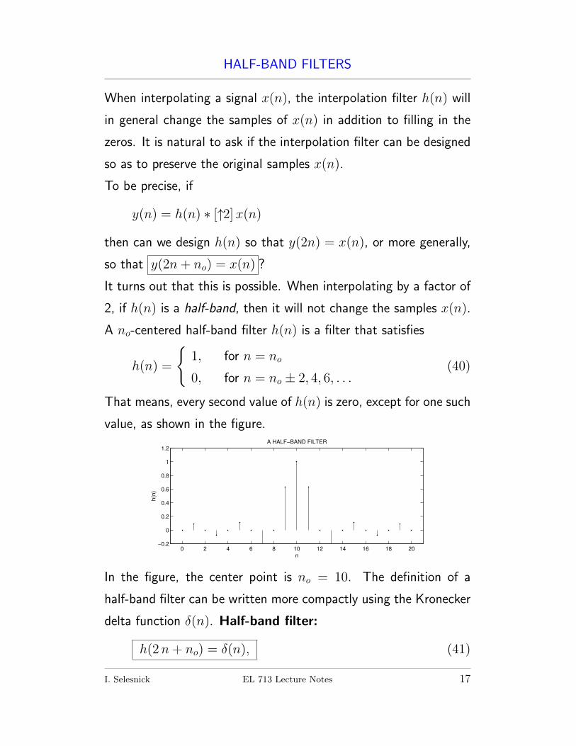
A no-centered half-band filter h(n) is a filter that satisfies

h(n) =

{1, for n = no

0, for n = no ± 2, 4, 6, . . .(40)

That means, every second value of h(n) is zero, except for one such

value, as shown in the figure.

0 2 4 6 8 10 12 14 16 18 20−0.2

0

0.2

0.4

0.6

0.8

1

1.2

n

h(n

)

A HALF−BAND FILTER

In the figure, the center point is no = 10. The definition of a

half-band filter can be written more compactly using the Kronecker

delta function δ(n). Half-band filter:

h(2n+ no) = δ(n), (41)


when no = 0, we get simply:

h(2n) = δ(n). (42)

Note that the transfer function of a half-band filter (centered at

no = 0) can be written as

H(z) = 1 + z−1H1(z2). (43)

Here H1(z) contains the odd samples of h(n).

NYQUIST FILTERS

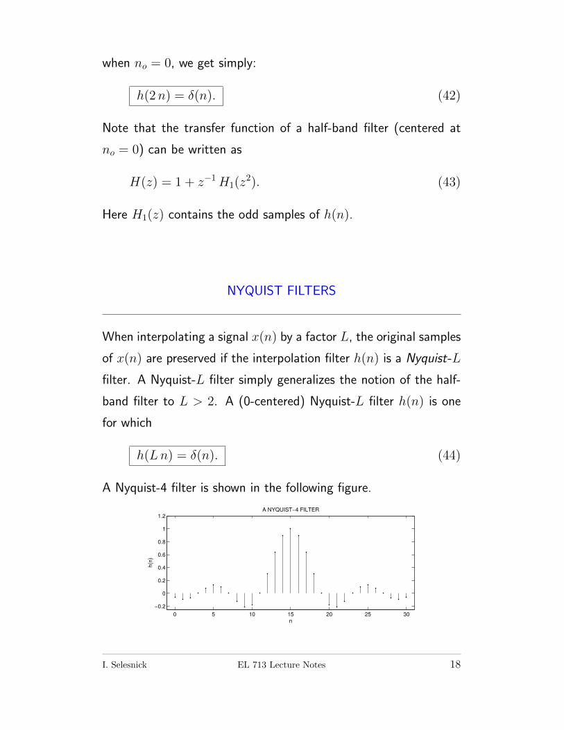
When interpolating a signal x(n) by a factor L, the original samples

of x(n) are preserved if the interpolation filter h(n) is a Nyquist-L

filter. A Nyquist-L filter simply generalizes the notion of the half-

band filter to L > 2. A (0-centered) Nyquist-L filter h(n) is one

for which

h(Ln) = δ(n). (44)

A Nyquist-4 filter is shown in the following figure.

0 5 10 15 20 25 30

−0.2

0

0.2

0.4

0.6

0.8

1

1.2

n

h(n

)

A NYQUIST−4 FILTER


THE NOBLE IDENTITY FOR THE UP-SAMPLER

The two following equivalences are sometimes called the noble iden-

tities.

Can you reverse the order of an up-sampler and a filter?

Yes and no — it depends. There are two cases.

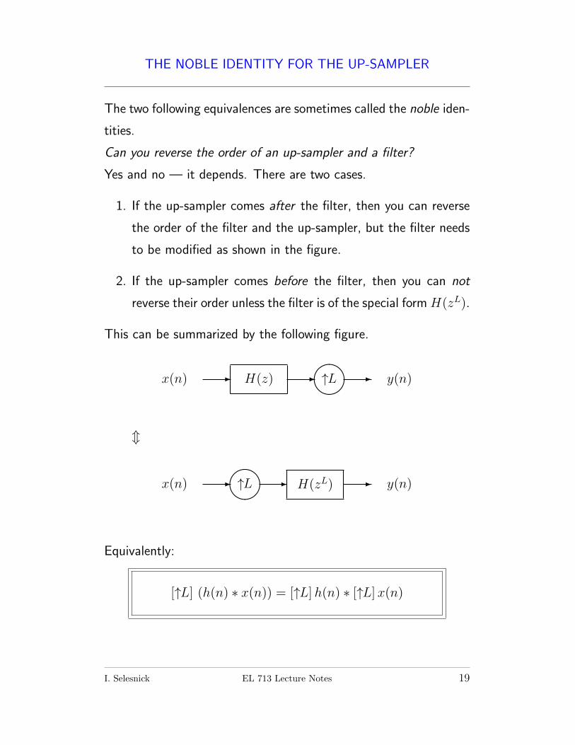
1. If the up-sampler comes after the filter, then you can reverse

the order of the filter and the up-sampler, but the filter needs

to be modified as shown in the figure.

2. If the up-sampler comes before the filter, then you can not

reverse their order unless the filter is of the special form H(zL).

This can be summarized by the following figure.

x(n) - H(z) -��↑L - y(n)

m

x(n) -��↑L - H(zL) - y(n)

Equivalently:

[↑L] (h(n) ∗ x(n)) = [↑L]h(n) ∗ [↑L]x(n)


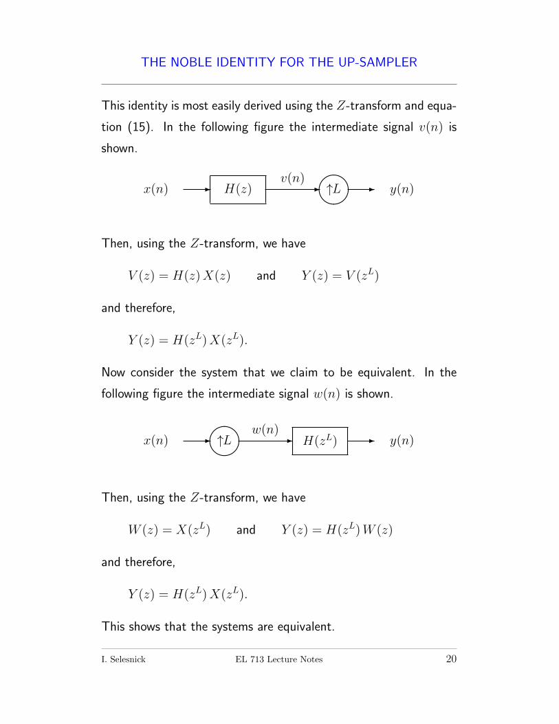
THE NOBLE IDENTITY FOR THE UP-SAMPLER

This identity is most easily derived using the Z-transform and equa-

tion (15). In the following figure the intermediate signal v(n) is

shown.

x(n) - H(z) -v(n)

��↑L - y(n)

Then, using the Z-transform, we have

V (z) = H(z)X(z) and Y (z) = V (zL)

and therefore,

Y (z) = H(zL)X(zL).

Now consider the system that we claim to be equivalent. In the

following figure the intermediate signal w(n) is shown.

x(n) -��↑L -

w(n)H(zL) - y(n)


W (z) = X(zL) and Y (z) = H(zL)W (z)

and therefore,

Y (z) = H(zL)X(zL).

This shows that the systems are equivalent.


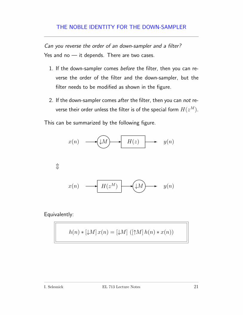
THE NOBLE IDENTITY FOR THE DOWN-SAMPLER

Can you reverse the order of an down-sampler and a filter?

Yes and no — it depends. There are two cases.

1. If the down-sampler comes before the filter, then you can re-

verse the order of the filter and the down-sampler, but the

filter needs to be modified as shown in the figure.

2. If the down-sampler comes after the filter, then you can not re-

verse their order unless the filter is of the special form H(zM).

This can be summarized by the following figure.

x(n) -��↓M - H(z) - y(n)

m

x(n) - H(zM) -��↓M - y(n)

Equivalently:

h(n) ∗ [↓M ]x(n) = [↓M ] ([↑M ]h(n) ∗ x(n))


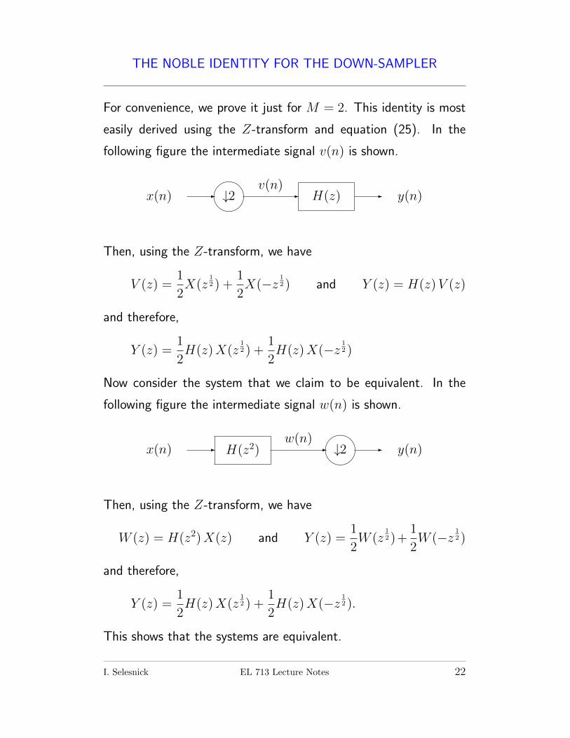
THE NOBLE IDENTITY FOR THE DOWN-SAMPLER

For convenience, we prove it just for M = 2. This identity is most

easily derived using the Z-transform and equation (25). In the

following figure the intermediate signal v(n) is shown.

x(n) -��↓2 -

v(n)H(z) - y(n)


V (z) =1

2X(z

12 ) +

1

2X(−z

12 ) and Y (z) = H(z)V (z)

and therefore,

Y (z) =1

2H(z)X(z

12 ) +

1

2H(z)X(−z

12 )

Now consider the system that we claim to be equivalent. In the

following figure the intermediate signal w(n) is shown.

x(n) - H(z2) -w(n)

��↓2 - y(n)


W (z) = H(z2)X(z) and Y (z) =1

2W (z

12 )+

1

2W (−z

12 )

and therefore,

Y (z) =1

2H(z)X(z

12 ) +

1

2H(z)X(−z

12 ).

This shows that the systems are equivalent.


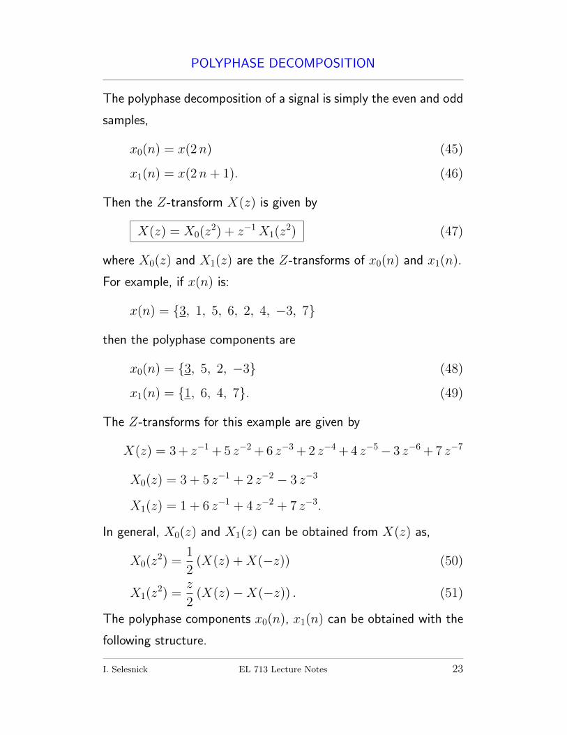
POLYPHASE DECOMPOSITION

The polyphase decomposition of a signal is simply the even and odd

samples,

x0(n) = x(2n) (45)

x1(n) = x(2n+ 1). (46)

Then the Z-transform X(z) is given by

X(z) = X0(z2) + z−1X1(z

2) (47)

where X0(z) and X1(z) are the Z-transforms of x0(n) and x1(n).

For example, if x(n) is:

x(n) = {3, 1, 5, 6, 2, 4, −3, 7}

then the polyphase components are

x0(n) = {3, 5, 2, −3} (48)

x1(n) = {1, 6, 4, 7}. (49)

The Z-transforms for this example are given by

X(z) = 3+ z−1+5 z−2+6 z−3+2 z−4+4 z−5− 3 z−6+7 z−7

X0(z) = 3 + 5 z−1 + 2 z−2 − 3 z−3

X1(z) = 1 + 6 z−1 + 4 z−2 + 7 z−3.

In general, X0(z) and X1(z) can be obtained from X(z) as,

X0(z2) =

1

2(X(z) +X(−z)) (50)

X1(z2) =

z

2(X(z)−X(−z)) . (51)

The polyphase components x0(n), x1(n) can be obtained with the

following structure.


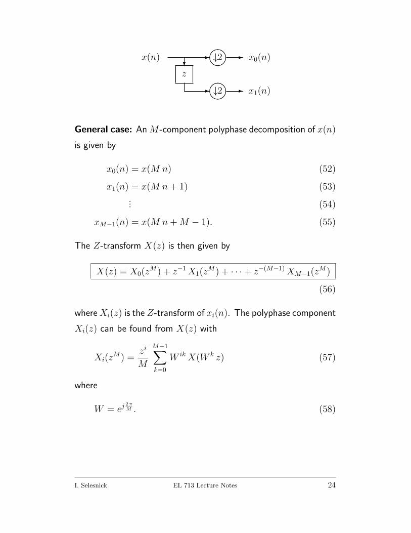
x(n) -��↓2 -

x1(n)

?

z

-��↓2 -

x0(n)

General case: An M -component polyphase decomposition of x(n)

is given by

x0(n) = x(M n) (52)

x1(n) = x(M n+ 1) (53)

... (54)

xM−1(n) = x(M n+M − 1). (55)

The Z-transform X(z) is then given by

X(z) = X0(zM) + z−1X1(z

M) + · · ·+ z−(M−1)XM−1(zM)

(56)

where Xi(z) is the Z-transform of xi(n). The polyphase component

Xi(z) can be found from X(z) with

Xi(zM) =

zi

M

M−1∑k=0

W ikX(W k z) (57)

where

W = ej2πM . (58)


EFFICIENT IMPLEMENTATION

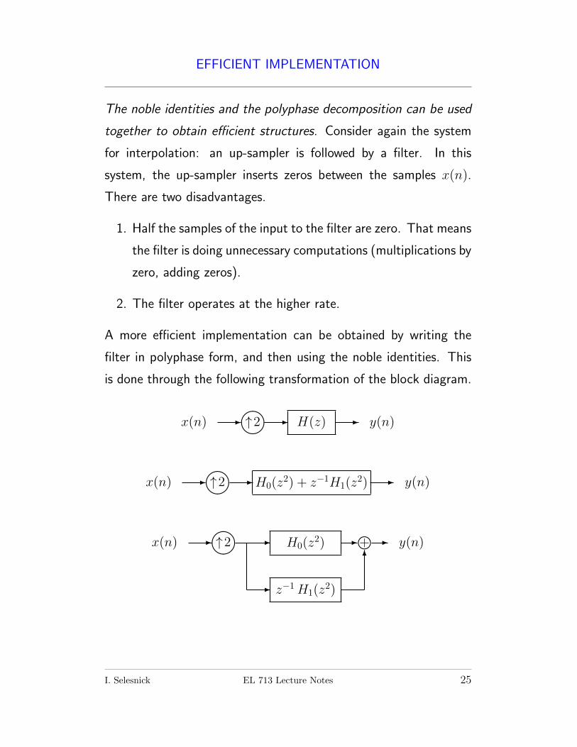
The noble identities and the polyphase decomposition can be used

together to obtain efficient structures. Consider again the system

for interpolation: an up-sampler is followed by a filter. In this

system, the up-sampler inserts zeros between the samples x(n).

There are two disadvantages.

1. Half the samples of the input to the filter are zero. That means

the filter is doing unnecessary computations (multiplications by

zero, adding zeros).

2. The filter operates at the higher rate.

A more efficient implementation can be obtained by writing the

filter in polyphase form, and then using the noble identities. This

is done through the following transformation of the block diagram.

x(n) -��↑2 - H(z) - y(n)

x(n) -��↑2 -H0(z

2) + z−1H1(z2) - y(n)

x(n) -��↑2 - H0(z

2) - l+ -

- z−1H1(z2)

6

y(n)


EFFICIENT IMPLEMENTATION

x(n) -��↑2 - H0(z

2) - l+ -

-��↑2 - z−1H1(z

2)

6

y(n)

x(n) -��↑2 - H0(z

2) - l+ -

-��↑2 - H1(z

2)

6

z−1

y(n)

x(n) - H0(z) -��↑2 - l+ -

- H1(z) -��↑2

6

z−1

6

y(n)

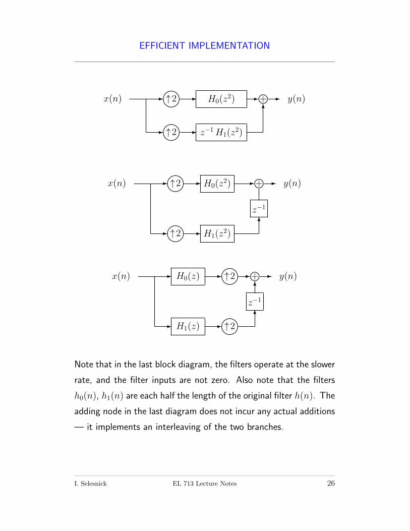
Note that in the last block diagram, the filters operate at the slower

rate, and the filter inputs are not zero. Also note that the filters

h0(n), h1(n) are each half the length of the original filter h(n). The

adding node in the last diagram does not incur any actual additions

— it implements an interleaving of the two branches.


HALF-BAND CASE

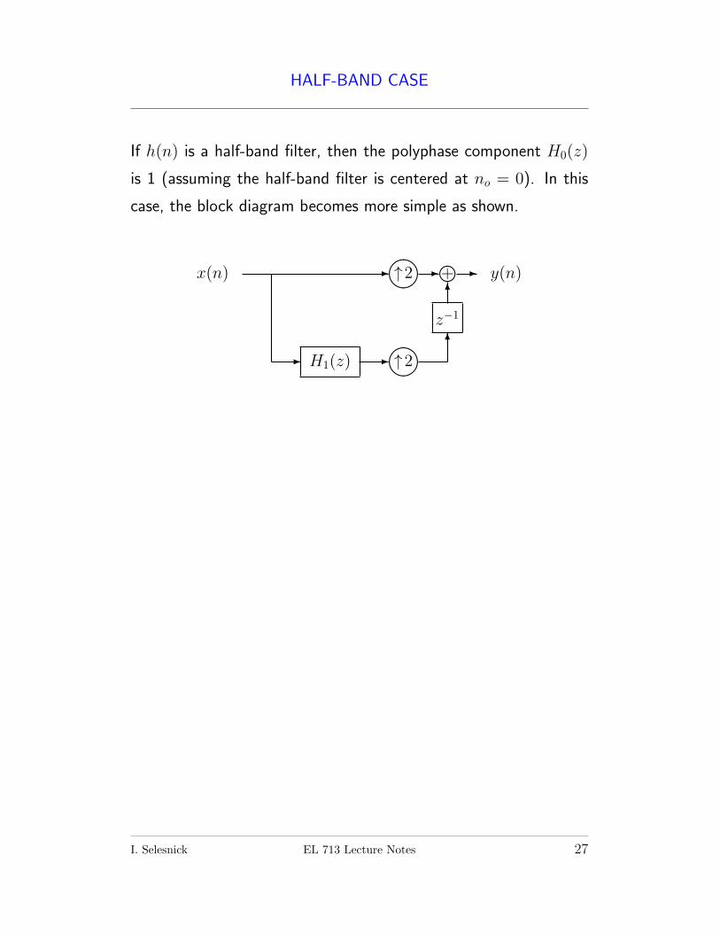
If h(n) is a half-band filter, then the polyphase component H0(z)

is 1 (assuming the half-band filter is centered at no = 0). In this

case, the block diagram becomes more simple as shown.

x(n) -��↑2 - l+ -

- H1(z) -��↑2

6

z−1

6

y(n)


POLYNOMIAL SIGNALS

A (discrete-time) polynomial signal x(n) is a signal of the form

x(n) = c0 + c1 n+ c2 n2 + · · ·+ cd n

d.

The degree is d. The set of polynomial signals of degree d or less

is denoted by Pd.Consider a system described by the rule

y(n) = x(n)− x(n− 1).

This system gives the first difference of the signal x(n). It has the

impulse response

h(n) = δ(n)− δ(n− 1),

and the transfer function

H(z) = 1− z−1

and so we can write

y(n) = h(n) ∗ x(n)

or

Y (z) =(1− z−1

)X(z).

Clearly if x(n) is a constant signal (x(n) = c, so we can write

x(n) ∈ P0), then the first difference of x(n) is identically zero,

Y (z) =(1− z−1

)X(z) = 0 for x(n) ∈ P0.

Moreover, the first difference Y (z) is identically zero only if x(n)

is a constant signal.


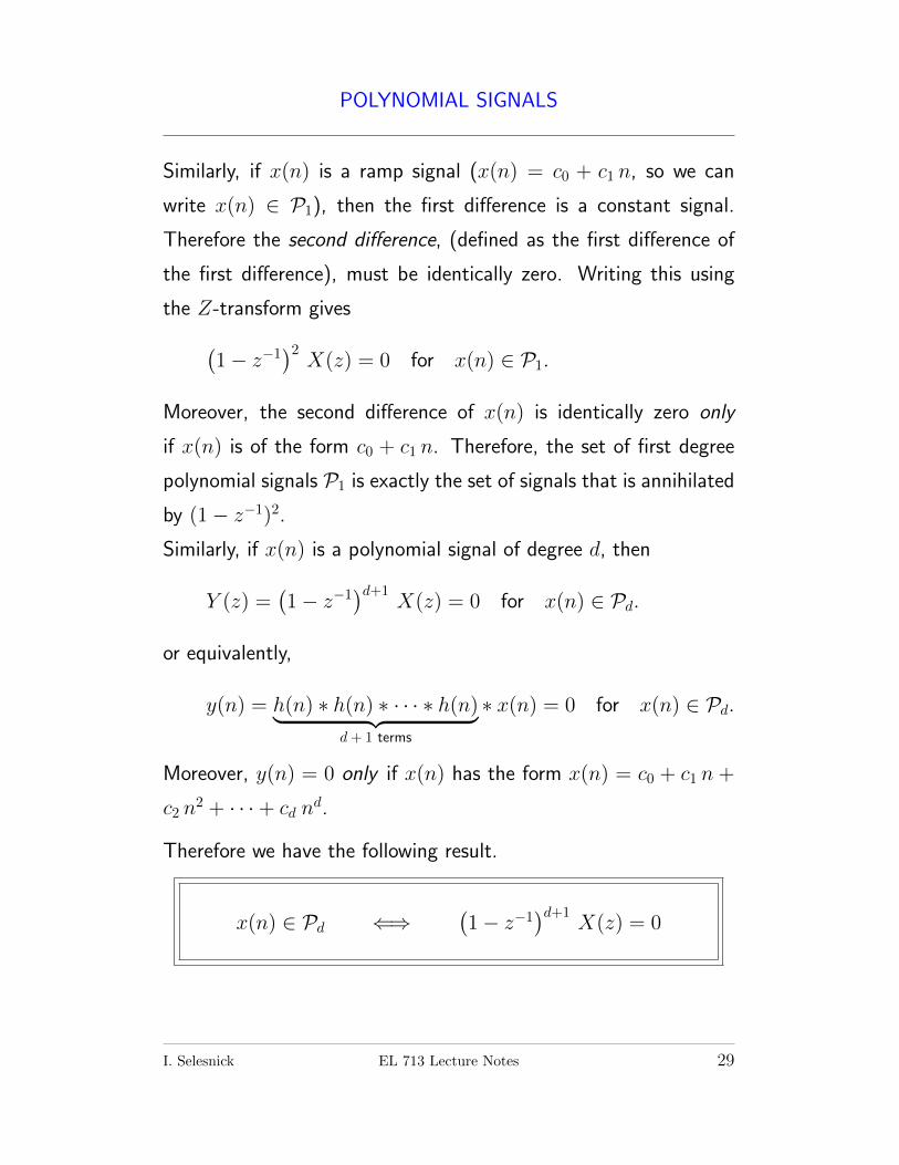
POLYNOMIAL SIGNALS

Similarly, if x(n) is a ramp signal (x(n) = c0 + c1 n, so we can

write x(n) ∈ P1), then the first difference is a constant signal.

Therefore the second difference, (defined as the first difference of

the first difference), must be identically zero. Writing this using

the Z-transform gives(1− z−1

)2X(z) = 0 for x(n) ∈ P1.

Moreover, the second difference of x(n) is identically zero only

if x(n) is of the form c0 + c1 n. Therefore, the set of first degree

polynomial signals P1 is exactly the set of signals that is annihilated

by (1− z−1)2.

Similarly, if x(n) is a polynomial signal of degree d, then

Y (z) =(1− z−1

)d+1X(z) = 0 for x(n) ∈ Pd.

or equivalently,

y(n) = h(n) ∗ h(n) ∗ · · · ∗ h(n)︸︷︷︸d+ 1 terms

∗ x(n) = 0 for x(n) ∈ Pd.

Moreover, y(n) = 0 only if x(n) has the form x(n) = c0 + c1 n +

c2 n2 + · · ·+ cd n

d.

Therefore we have the following result.

x(n) ∈ Pd ⇐⇒(1− z−1

)d+1X(z) = 0


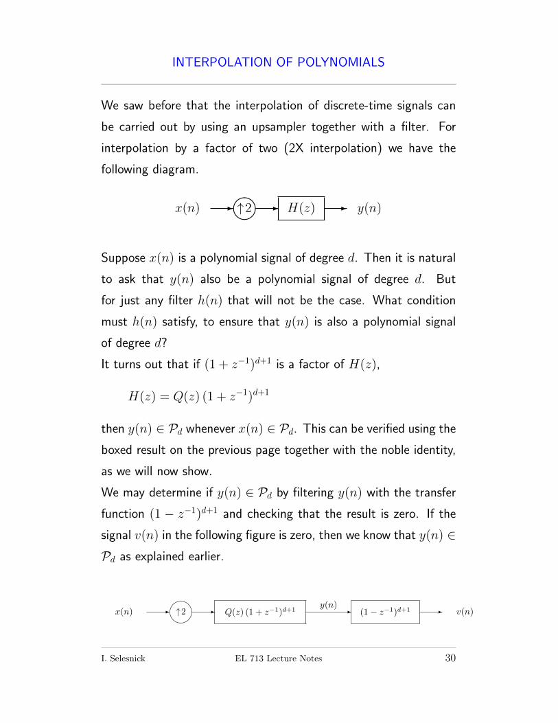
INTERPOLATION OF POLYNOMIALS

We saw before that the interpolation of discrete-time signals can

be carried out by using an upsampler together with a filter. For

interpolation by a factor of two (2X interpolation) we have the

following diagram.

x(n) -��↑2 - H(z) - y(n)

Suppose x(n) is a polynomial signal of degree d. Then it is natural

to ask that y(n) also be a polynomial signal of degree d. But

for just any filter h(n) that will not be the case. What condition

must h(n) satisfy, to ensure that y(n) is also a polynomial signal

of degree d?

It turns out that if (1 + z−1)d+1 is a factor of H(z),

H(z) = Q(z) (1 + z−1)d+1

then y(n) ∈ Pd whenever x(n) ∈ Pd. This can be verified using the

boxed result on the previous page together with the noble identity,

as we will now show.

We may determine if y(n) ∈ Pd by filtering y(n) with the transfer

function (1 − z−1)d+1 and checking that the result is zero. If the

signal v(n) in the following figure is zero, then we know that y(n) ∈Pd as explained earlier.

x(n) -��↑2 - Q(z) (1 + z−1)d+1 -

y(n)(1− z−1)d+1 - v(n)


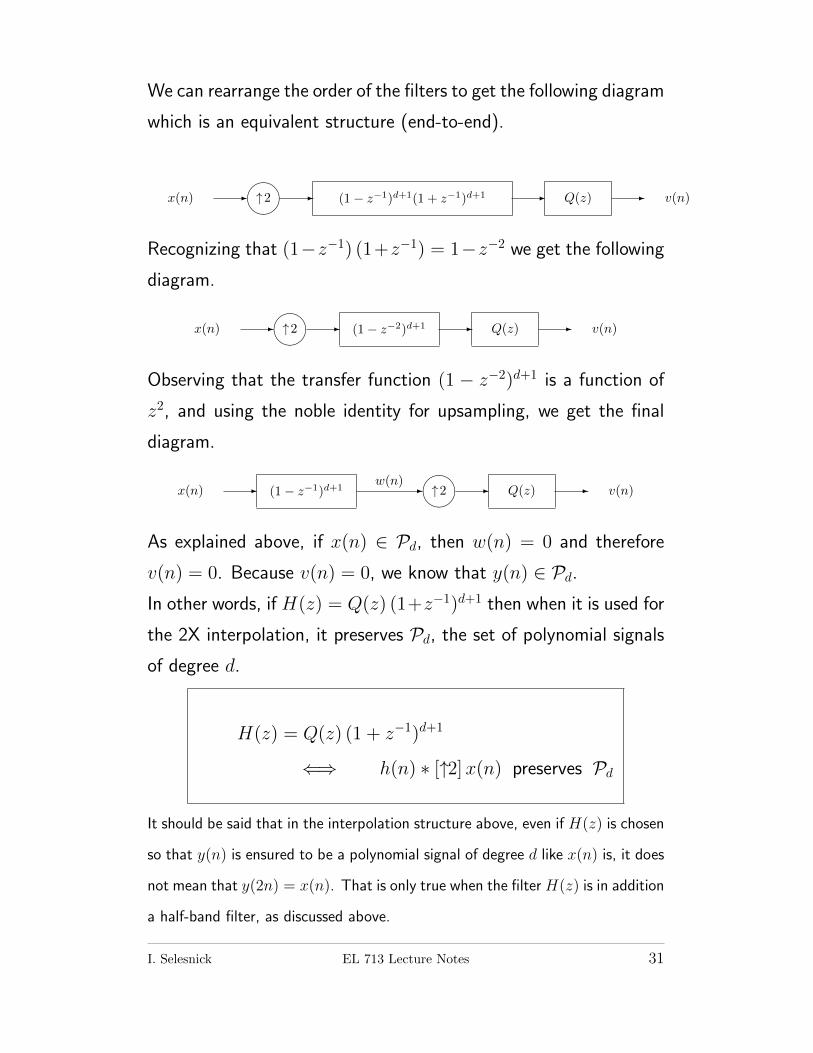
We can rearrange the order of the filters to get the following diagram

which is an equivalent structure (end-to-end).

x(n) -��↑2 - (1− z−1)d+1(1 + z−1)d+1 - Q(z) - v(n)

Recognizing that (1−z−1) (1+z−1) = 1−z−2 we get the following

diagram.

x(n) -��↑2 - (1− z−2)d+1 - Q(z) - v(n)

Observing that the transfer function (1 − z−2)d+1 is a function of

z2, and using the noble identity for upsampling, we get the final

diagram.

x(n) - (1− z−1)d+1 -w(n) ��↑2 - Q(z) - v(n)

As explained above, if x(n) ∈ Pd, then w(n) = 0 and therefore

v(n) = 0. Because v(n) = 0, we know that y(n) ∈ Pd.In other words, if H(z) = Q(z) (1+z−1)d+1 then when it is used for

the 2X interpolation, it preserves Pd, the set of polynomial signals

of degree d.

H(z) = Q(z) (1 + z−1)d+1

⇐⇒ h(n) ∗ [↑2]x(n) preserves Pd

It should be said that in the interpolation structure above, even if H(z) is chosen

so that y(n) is ensured to be a polynomial signal of degree d like x(n) is, it does

not mean that y(2n) = x(n). That is only true when the filter H(z) is in addition

a half-band filter, as discussed above.


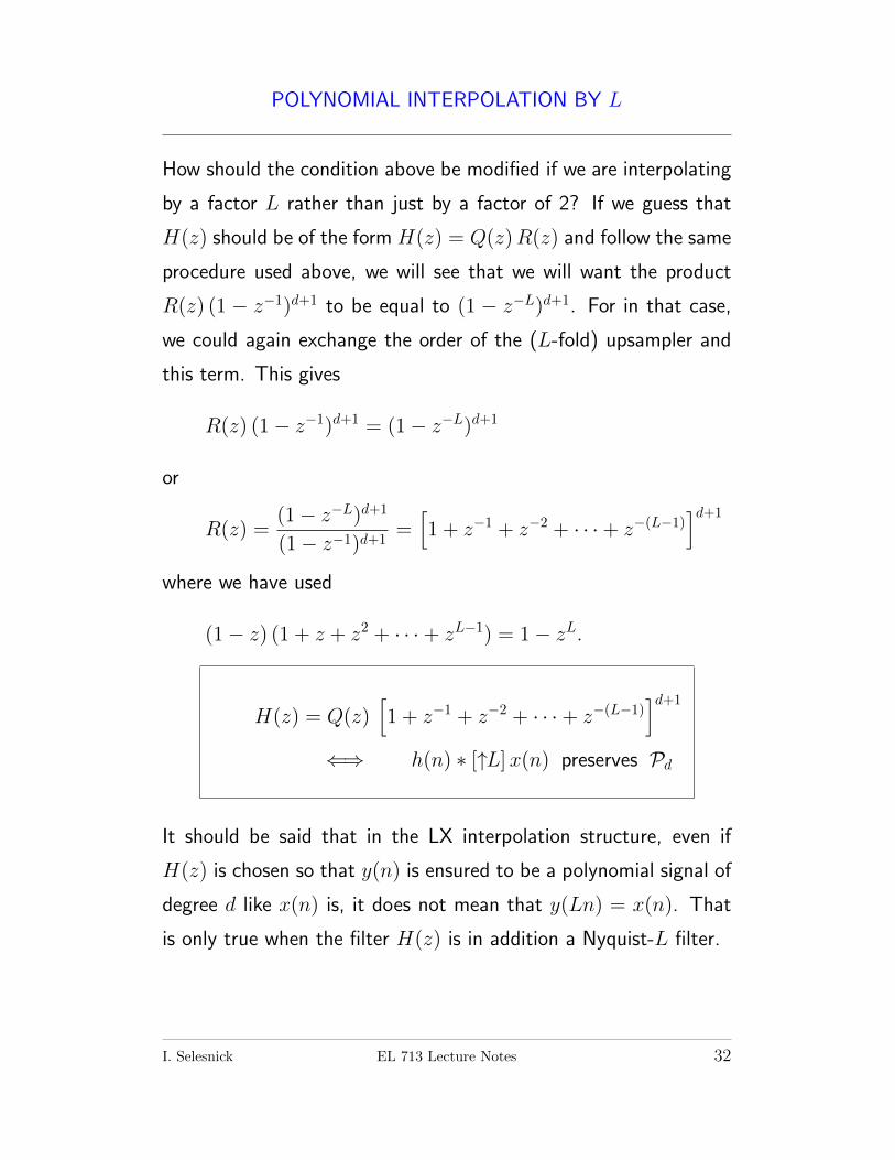
POLYNOMIAL INTERPOLATION BY L

How should the condition above be modified if we are interpolating

by a factor L rather than just by a factor of 2? If we guess that

H(z) should be of the form H(z) = Q(z)R(z) and follow the same

procedure used above, we will see that we will want the product

R(z) (1 − z−1)d+1 to be equal to (1 − z−L)d+1. For in that case,

we could again exchange the order of the (L-fold) upsampler and

this term. This gives

R(z) (1− z−1)d+1 = (1− z−L)d+1

or

R(z) =(1− z−L)d+1

(1− z−1)d+1=[1 + z−1 + z−2 + · · ·+ z−(L−1)

]d+1

where we have used

(1− z) (1 + z + z2 + · · ·+ zL−1) = 1− zL.

H(z) = Q(z)[1 + z−1 + z−2 + · · ·+ z−(L−1)

]d+1

⇐⇒ h(n) ∗ [↑L]x(n) preserves Pd

It should be said that in the LX interpolation structure, even if

H(z) is chosen so that y(n) is ensured to be a polynomial signal of

degree d like x(n) is, it does not mean that y(Ln) = x(n). That

is only true when the filter H(z) is in addition a Nyquist-L filter.


Documents

MULTIRATE SIGNAL PROCESSING - NYU Tandon …eeweb.poly.edu/iselesni/EL713/zoom/mrate.pdf · MULTIRATE SIGNAL PROCESSING 1.APPLICATIONS ... is de ned by the relation y(n) = ... 6;0;:::g: