1

Multiresolution Image Classi�cation by Hierarchical

Modeling with Two Dimensional Hidden Markov

Models

Jia Li, Member, IEEE, Robert M. Gray, Fellow, IEEE, and

Richard A. Olshen, Senior Member, IEEE

Abstract

The paper treats a multiresolution hidden Markov model (MHMM) for classifying images. Each image is

represented by feature vectors at several resolutions, which are statistically dependent as modeled by the under-

lying state process, a multiscale Markov mesh. Unknowns in the model are estimated by maximum likelihood,

in particular by employing the EM algorithm. An image is classi�ed by �nding the optimal set of states with

maximum a posteriori probability (MAP). States are then mapped into classes. The multiresolution model

enables multiscale information about context to be incorporated into classi�cation. Suboptimal algorithms

based on the model provide progressive classi�cation which is much faster than the algorithm based on single

resolution HMMs.

Keywords

image classi�cation, image segmentation, two dimensional multiresolution hidden Markov model, EM algo-

rithm, tests of goodness of �t

I. Introduction

Recent years have seen substantial interest and activity devoted to algorithms for multiresolution process-

ing [16], [37]. One reason for this focus on image segmentation is that multiresolution processing seems to

This work was supported by the National Science Foundation under NSF Grant No. MIP-9706284. Jia Li is with the XeroxPalo Alto Research Center, Palo Alto, CA 94304. Robert M. Gray is with the Information Systems Laboratory, Department ofElectrical Engineering; and Richard A. Olshen is with the Department of Health Research and Policy, Stanford University, CA94305, U.S.A. Email: jiali@isl.stanford.edu, rmgray@stanford.edu, olshen@stat.stanford.edu.

2

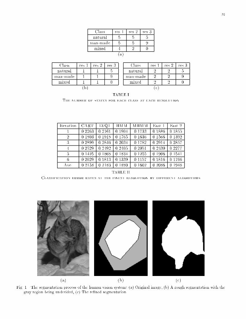
imitate the decision procedure of the human vision system (HVS) [28]. For example, when the HVS segments

a picture shown in Fig. 1 into a foreground region (a fox) and a background region, the foreground can be

located roughly by a brief glance which is similar to viewing a low resolution image. As is shown in Fig. 1(b),

the crude decision leaves only a small unsure area around the boundary. Further careful examination of de-

tails at the boundary results in the �nal decision as to what is important in the image. Both global and local

information are used by the HVS, which distributes e�ort unevenly by looking at more ambiguous regions at

higher resolutions than it devotes to other regions.

Context-dependent classi�cation algorithms based on two dimensional hidden Markov models (2-D HMMs)

have been developed [14], [24], [25] to overcome the over-localization of conventional block-based classi�cation

algorithms. In this paper, a multiresolution extension of the 2-D HMM described in [25] is proposed so that

more global context information can be used e�ciently. A joint decision on classes for the entire image is needed

to classify optimally an image based on the 2-D HMM [25]. In real life, however, because of computational

complexity, we have to divide an image into subimages and ignore statistical dependence among the subimages.

With the increase of model complexity, it is necessary to decrease the size of the subimages to preserve modest

computational feasibility. Instead of using smaller subimages, a classi�er based on the multiresolution model

retains tractability by representing context information hierarchically.

With a 2-D multiresolution hidden Markov model (MHMM), an image is taken to be a collection of feature

vectors at several resolutions. These feature vectors at a particular resolution are determined only by the image

at that resolution. The feature vectors across all the resolutions are generated by a multiresolution Markov

source [35], [18]. As with the 2-D HMM, the source exists in a state at any block at any resolution. Given the

state of a block at each particular resolution, the feature vector is assumed to have a Gaussian distribution

so that the unconditional distribution is a Gaussian mixture. The parameters of each Gaussian distribution

depend on both state and resolution. At any �xed resolution, as with the 2-D HMM, the probability of the

source entering a particular state is governed by a second order Markov mesh [1]. Unlike the HMM, there

are multiple Markov meshes at one resolution whose transition probabilities depend on the states of parent

blocks.

3

Many other multiresolution models have been developed to represent statistical dependence among image

pixels, with wide applications in image segmentation, denoising, restoration, etc. The multiscale autoregres-

sive model proposed by Basseville et al. [3], the multiscale random �eld (MSRF) proposed by Bouman and

Shapiro [7], and the wavelet-domain HMM proposed by Crouse et al. [11] will be discussed and compared

with the 2-D MHMM in Section III after necessary notation is introduced in Section II.

As was mentioned, the human vision system is fast as well as accurate, at least by standards of automated

technologies, whereas the 2-D MHMM and other multiresolution models [3] do not necessarily bene�t classi-

�cation speed because information is combined from several resolutions in order to make a decision regarding

a local region. However, a 2-D MHMM provides a hierarchical structure for fast progressive classi�cation if

the maximum a posteriori classi�cation rule is relaxed. The progressive classi�er is inspired by the human

vision system to examine higher resolutions selectively for more ambiguous regions.

In Section II, a mathematical formulation of the basic assumptions of a 2-D multiresolution HMM is pro-

vided. Related work on multiresolution modeling for images is discussed in Section III. The algorithm is

presented in Section IV. Fast algorithms for progressive classi�cation are presented in Section V. Section VI

provides an analysis of computational complexity. Experiments with the algorithm are described in Sec-

tion VII. Section VIII is about hypothesis testing as it applies to determining the validity of the MHMMs.

Conclusions are drawn in Section IX.

II. Basic Assumptions of 2-D MHMM

To classify an image, representations of the image at di�erent resolutions are computed �rst. The original

image corresponds to the highest resolution. Lower resolutions are generated by successively �ltering out high

frequency information. Wavelet transforms [12] naturally provide low resolution images in the low frequency

band (the LL band). A sequence of images at several resolutions is shown in Fig. 2. As subsampling is applied

for every reduced resolution, the image size decreases by a factor of two in both directions. As is shown

by Fig. 2, the number of blocks in both rows and columns is successively diminished by half at each lower

resolution. Obviously, a block at a lower resolution covers a spatially more global region of the image. As

4

is indicated by Fig. 3, the block at the lower resolution is referred to as a parent block, and the four blocks

at the same spatial location at the higher resolution are referred to as child blocks. We will always assume

such a \quadtree" split in the sequel since the training and testing algorithms can be easily extended to other

hierarchical structures.

We �rst review the basic assumptions of the single resolution 2-D HMM as presented in [25]. In the 2-D

HMM, feature vectors are generated by a Markov model that may change state once every block. Suppose

there are M states, the state of block (i; j) being denoted by si;j . The feature vector of block (i; j) is ui;j ,

and the class is ci;j . We use P (�) to represent the probability of an event. We denote (i0; j0) < (i; j) if i0 < i

or i0 = i; j 0 < j, in which case we say that block (i0; j0) is before block (i; j). The �rst assumption is that

P (si;j j context) = am;n;l ;

context = fsi0;j0 ; ui0;j0 : (i0; j0) < (i; j)g ;

where m = si�1;j , n = si;j�1, and l = si;j . The second assumption is that for every state, the feature

vectors follow a Gaussian distribution. Once the state of a block is known, the feature vector is conditionally

independent of information in other blocks. The covariance matrix �s and the mean vector �s of the Gaussian

distribution vary with state s.

For the MHMM, denote the collection of resolutions byR = f1; :::; Rg, with r = R being the �nest resolution.

Let the collection of block indices at resolution r be

N(r) = f(i; j) : 0 � i < w=2R�r; 0 � j < z=2R�rg :

Images are described by feature vectors at all the resolutions, denoted by u(r)i;j , r 2 R. Every feature vector is

labeled with a class c(r)i;j . The underlying state of a feature vector is s

(r)i;j . At each resolution r, the set of states

is f1(r); 2(r); :::;M(r)r g. Note that as states vary across resolutions, di�erent resolutions do not share states.

As with the single resolution model, each state at every resolution is uniquely mapped to one class. On

5

the other hand, a block with a known class may exist in several states. Since a block at a lower resolution

contains several blocks at a higher resolution, it may not be of a pure class. Therefore, except for the highest

resolution, there is an extra \mixed" class in addition to the original classes. Denote the set of original classes

by G = f1; 2; :::; Gg and the \mixed" class by G + 1. Because of the unique mapping between states and

classes, the state of a parent block may constrain the possible states for its child blocks. If the state of a

parent block is mapped to a determined (non-mixed) class, the child blocks can exist only in states that map

to the same class.

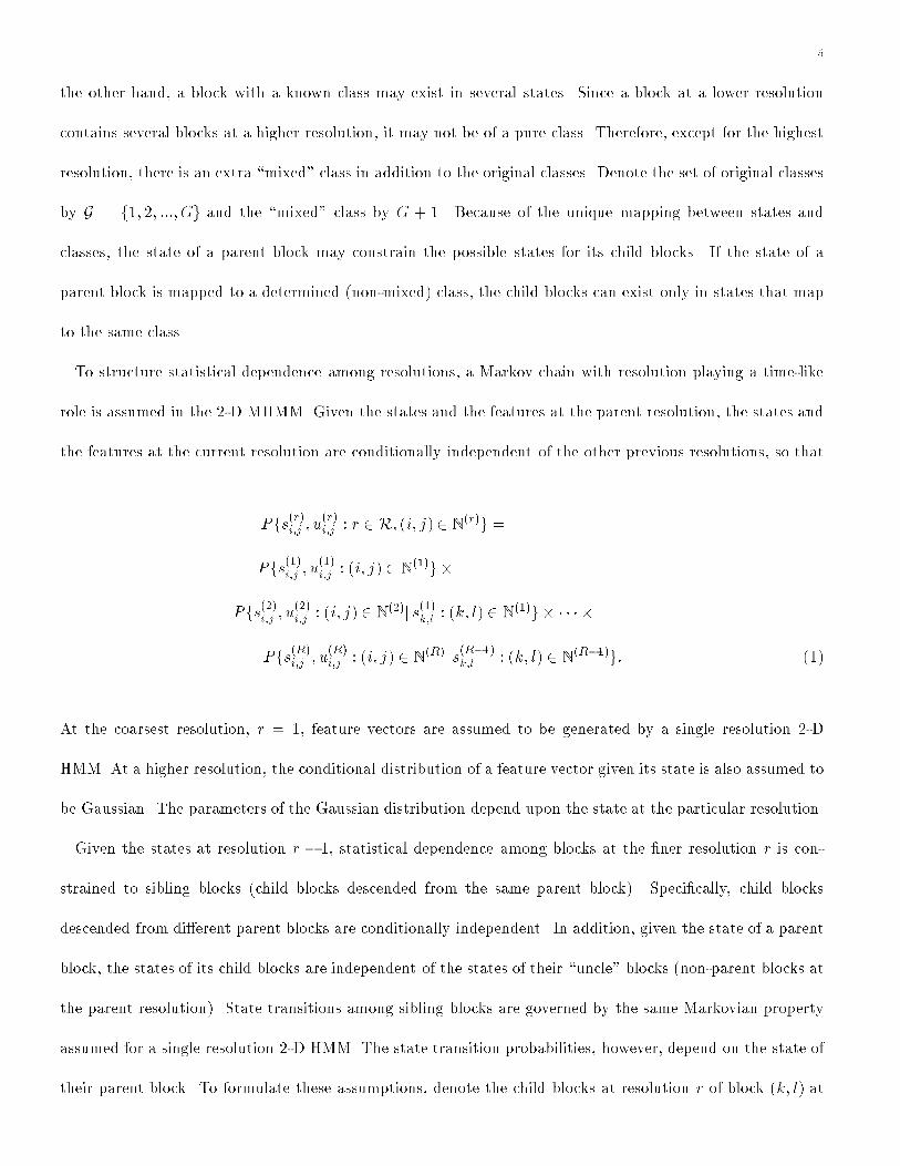
To structure statistical dependence among resolutions, a Markov chain with resolution playing a time-like

role is assumed in the 2-D MHMM. Given the states and the features at the parent resolution, the states and

the features at the current resolution are conditionally independent of the other previous resolutions, so that

Pfs(r)i;j ; u

(r)i;j : r 2 R; (i; j)2 N

(r)g =

Pfs(1)i;j ; u

(1)i;j : (i; j) 2 N

(1)g �

Pfs(2)i;j ; u(2)i;j : (i; j) 2 N

(2)j s(1)k;l

: (k; l) 2 N(1)g � � � � �

Pfs(R)i;j ; u

(R)i;j : (i; j) 2 N

(R)j s(R�1)k;l

: (k; l) 2 N(R�1)g: (1)

At the coarsest resolution, r = 1, feature vectors are assumed to be generated by a single resolution 2-D

HMM. At a higher resolution, the conditional distribution of a feature vector given its state is also assumed to

be Gaussian. The parameters of the Gaussian distribution depend upon the state at the particular resolution.

Given the states at resolution r � 1, statistical dependence among blocks at the �ner resolution r is con-

strained to sibling blocks (child blocks descended from the same parent block). Speci�cally, child blocks

descended from di�erent parent blocks are conditionally independent. In addition, given the state of a parent

block, the states of its child blocks are independent of the states of their \uncle" blocks (non-parent blocks at

the parent resolution). State transitions among sibling blocks are governed by the same Markovian property

assumed for a single resolution 2-D HMM. The state transition probabilities, however, depend on the state of

their parent block. To formulate these assumptions, denote the child blocks at resolution r of block (k; l) at

6

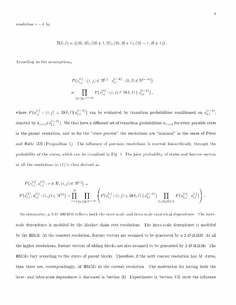
resolution r � 1 by

D(k; l) = f(2k; 2l); (2k+ 1; 2l); (2k; 2l+ 1); (2k+ 1; 2l+ 1)g :

According to the assumptions,

Pfs(r)i;j : (i; j) 2 N

(r) j s(r�1)k;l

: (k; l) 2 N(r�1)g

=Y

(k;l)2N(r�1)

Pfs(r)i;j : (i; j) 2 D (k; l) j s

(r�1)k;l g ;

where Pfs(r)i;j : (i; j) 2 D (k; l)j s

(r�1)k;l

g can be evaluated by transition probabilities conditioned on s(r�1)k;l

,

denoted by am;n;l(s(r�1)k;l

). We thus have a di�erent set of transition probabilities am;n;l for every possible state

in the parent resolution, and so for the \state process" the resolutions are \minimal" in the sense of P�erez

and Heitz [33] (Proposition 1). The in uence of previous resolutions is exerted hierarchically through the

probability of the states, which can be visualized in Fig. 4. The joint probability of states and feature vectors

at all the resolutions in (1) is then derived as

Pfs(r)i;j ; u

(r)i;j : r 2 R; (i; j)2 N

(r)g =

Pfs(1)i;j ; u

(1)i;j : (i; j) 2 N

(1)g �RYr=2

Y(k;l)2N(r�1)

0@Pfs(r)i;j : (i; j) 2 D(k; l) j s

(r�1)k;l g

Y(i;j)2D(k;l)

Pfu(r)i;j j s

(r)i;j g

1A :

To summarize, a 2-D MHMM re ects both the inter-scale and intra-scale statistical dependence. The inter-

scale dependence is modeled by the Markov chain over resolutions. The intra-scale dependence is modeled

by the HMM. At the coarsest resolution, feature vectors are assumed to be generated by a 2-D HMM. At all

the higher resolutions, feature vectors of sibling blocks are also assumed to be generated by 2-D HMMs. The

HMMs vary according to the states of parent blocks. Therefore, if the next coarser resolution has M states,

then there are, correspondingly, M HMMs at the current resolution. The motivation for having both the

inter- and intra-scale dependence is discussed in Section III. Experiments in Section VII show the in uence

7

of both types of dependence.

III. Related Work

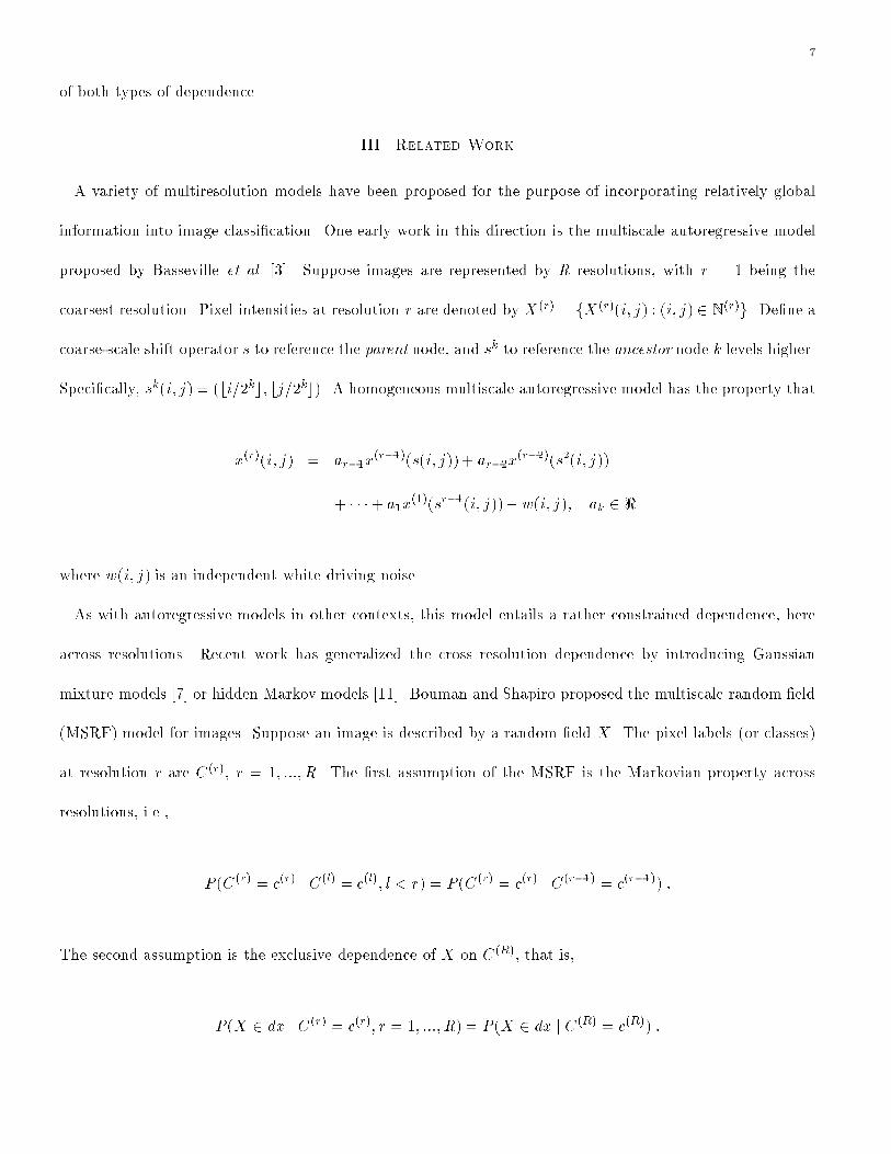
A variety of multiresolution models have been proposed for the purpose of incorporating relatively global

information into image classi�cation. One early work in this direction is the multiscale autoregressive model

proposed by Basseville et al. [3]. Suppose images are represented by R resolutions, with r = 1 being the

coarsest resolution. Pixel intensities at resolution r are denoted by X(r) = fX(r)(i; j) : (i; j) 2 N(r)g. De�ne a

coarse-scale shift operator s to reference the parent node, and sk to reference the ancestor node k levels higher.

Speci�cally, sk(i; j) = (bi=2kc; bj=2kc). A homogeneous multiscale autoregressive model has the property that

x(r)(i; j) = ar�1x(r�1)(s(i; j)) + ar�2x

(r�2)(s2(i; j))

+ � � �+ a1x(1)(sr�1(i; j))+ w(i; j); ak 2 <

where w(i; j) is an independent white driving noise.

As with autoregressive models in other contexts, this model entails a rather constrained dependence, here

across resolutions. Recent work has generalized the cross resolution dependence by introducing Gaussian

mixture models [7] or hidden Markov models [11]. Bouman and Shapiro proposed the multiscale random �eld

(MSRF) model for images. Suppose an image is described by a random �eld X . The pixel labels (or classes)

at resolution r are C(r), r = 1; :::; R. The �rst assumption of the MSRF is the Markovian property across

resolutions, i.e.,

P (C(r) = c(r) j C(l) = c(l); l < r) = P (C(r) = c(r) j C(r�1) = c(r�1)) :

The second assumption is the exclusive dependence of X on C(R), that is,

P (X 2 dx j C(r) = c(r); r = 1; :::; R) = P (X 2 dx j C(R) = c(R)) :

8

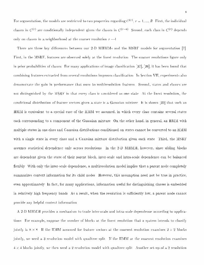
For segmentation, the models are restricted to two properties regarding C(r), r = 1; :::; R. First, the individual

classes in C(r) are conditionally independent given the classes in C(r�1). Second, each class in C(r) depends

only on classes in a neighborhood at the coarser resolution r � 1.

There are three key di�erences between our 2-D MHMMs and the MSRF models for segmentation [7].

First, in the MSRF, features are observed solely at the �nest resolution. The coarser resolutions �gure only

in prior probabilities of classes. For many applications of image classi�cation [37], [26], it has been found that

combining features extracted from several resolutions improves classi�cation. In Section VII, experiments also

demonstrate the gain in performance that owes to multiresolution features. Second, states and classes are

not distinguished by the MSRF in that every class is considered as one state. At the �nest resolution, the

conditional distribution of feature vectors given a state is a Gaussian mixture. It is shown [39] that such an

HMM is equivalent to a special case of the HMM we assumed, in which every class contains several states

each corresponding to a component of the Guassian mixture. On the other hand, in general, an HMM with

multiple states in one class and Gaussian distributions conditioned on states cannot be converted to an HMM

with a single state in every class and a Gaussian mixture distribution given each state. Third, the MSRF

assumes statistical dependence only across resolutions. In the 2-D MHMM, however, since sibling blocks

are dependent given the state of their parent block, inter-scale and intra-scale dependence can be balanced

exibly. With only the inter-scale dependence, a multiresolution model implies that a parent node completely

summarizes context information for its child nodes. However, this assumption need not be true in practice,

even approximately. In fact, for many applications, information useful for distinguishing classes is embedded

in relatively high frequency bands. As a result, when the resolution is su�ciently low, a parent node cannot

provide any helpful context information.

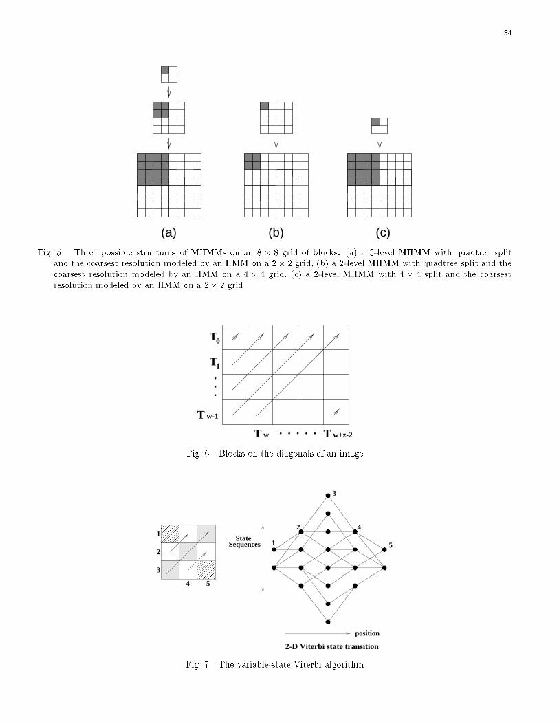
A 2-D MHMM provides a mechanism to trade inter-scale and intra-scale dependence according to applica-

tions. For example, suppose the number of blocks at the �nest resolution that a system intends to classify

jointly is 8 � 8. If the HMM assumed for feature vectors at the coarsest resolution examines 2 � 2 blocks

jointly, we need a 3 resolution model with quadtree split. If the HMM at the coarsest resolution examines

4� 4 blocks jointly, we then need a 2 resolution model with quadtree split. Another set-up of a 2 resolution

9

model might be to replace the quadtree split by a 4 � 4 split and assume an HMM on 2 � 2 blocks at the

coarse resolution. The three possibilities of the MHMM are shown in Figure 5. All the parameters in the

model structure set-up can be chosen conveniently as inputs to algorithms for training and testing.

Another multiresolution model based on HMMs is the model proposed for wavelet coe�cients by Crouse et

al. [11], where wavelet coe�cients across resolutions are assumed to be generated by one-dimensional hidden

Markov models with resolution being the time-like role in the Markov chain. If we view wavelet coe�cients

as special cases of features, the model in [11] considers features observed at multiple resolutions. However,

intra-scale dependence is not pursued in depth in [11]. This wavelet-domain model is applied to image

segmentation [9] and is extended to general features in [29].

The approach of applying models to image segmentation in [9] is di�erent from that of Bouman and

Shapiro [7] and ours. States in wavelet-domain HMMs are not related to classes. In particular, there are

two states at every resolution, one representing a wavelet coe�cient being large and the other small. To seg-

ment images, a separate HMM is trained for each class. A local region in an image is regarded as an instance

of a random process described by one of the HMMs. To decide the class of the local region, likelihood is

computed using the HMM of each class, and the class yielding the maximum likelihood is selected. The whole

image is then segmented by combining decisions for all the local regions. It is not straightforward for such an

approach to account for the spatial dependence among classes in an image. Furthermore, the wavelet-domain

HMMs alone do not provide a natural mechanism to incorporate segmentation results at multiple resolutions.

A remedy, speci�cally context-based interscale fusion, is developed in [9] to address this issue. In Bouman

and Shapiro [7] and our paper, however, an entire image is regarded as an instance of a 2-D random process

characterized by one model, which re ects the transition properties among classes/states at all the resolutions

as well as the dependence of feature vectors on classes/states. The set of classes or states with the maximum

a posteriori probability is sought according to the model. Segmenting an image by combining features at

multiple resolutions is inherent in our algorithm based on 2-D MHMMs. As the number of states and the

way of extracting features are allowed to vary with resolution, it is exible enough to incorporate multiscale

information for classi�cation using 2-D MHMMs.

10

In computer vision, there has been much work on learning vision by image modeling [20], [22], [17]. Partic-

ularly, in [17], multiresolution modeling is applied to estimate motions from image frames. Bayesian network

techniques [5], [32], [19] have played an important role in learning models in computer vision. Theories on

Bayesian network also provide guidance on how to construct models with tractable learning complexity. Exact

inference on general Bayesian networks is NP-hard, as discussed by Cooper [10]. Computationally e�cient

algorithms for training a general Bayesian network are not always available. As we have constructed 2-D MH-

MMs by extending 1-D HMMs used in speech recognition [39], e�cient algorithms for training and applying

2-D MHMMs are derived from the EM algorithm [13] and related techniques developed for speech recognition.

IV. The Algorithm

The parameters of the multiresolution model are estimated iteratively by the EM algorithm [13]. To

ease the enormous computational burden, we apply a suboptimal estimation procedure: the Viterbi training

algorithm [39]. At every iteration, the combination of states at all the resolutions with the maximum a

posteriori probability (MAP) is searched by the Viterbi algorithm [38]. These states are then assumed to

be real states to update the estimation of parameters. Because of the multiple resolutions, a certain part

of the training algorithm used for the single resolution HMM [25] is changed to a recursive procedure. For

completeness, we present the EM algorithm for estimating the parameters of a 2-D HMM as described in [25].

Next, the EM estimation is approximated by the Viterbi training algorithm, which is then extended to the

case of a 2-D MHMM.

For a single resolution HMM, suppose that the states are si;j , 1 � si;j � M , the class labels are ci;j , and

the feature vectors are ui;j , (i; j) 2 N, a generic index set. Denote:

1. the set of observed feature vectors for the entire image by u = fui;j : (i; j) 2 Ng;

2. the set of states for the image by s = fsi;j : (i; j) 2 Ng;

3. the set of classes for the image by c = fci;j : (i; j) 2 Ng;

4. the mapping from a state si;j to its class by C(si;j), and the set of classes mapped from states s by C(s);

and

11

5. the model estimated at iteration p by �(p).

The EM algorithm iteratively improves the model estimation by the following steps:

1. Given the current model estimate �(p), the observed feature vectors ui;j , and classes ci;j , (i; j) 2 N, the

mean vectors and covariance matrices are updated by

�(p+1)m =

Pi;j L

(p)m (i; j)ui;jP

i;j L(p)m (i; j)

(2)

�(p+1)m =

Pi;j L

(p)m (i; j)(ui;j � �

(p+1)m )(ui;j � �

(p+1)m )tP

i;j L(p)m (i; j)

: (3)

L(p)m (i; j) is the posteriori probability of block (i; j) being in state m, calculated by

L(p)m (i; j) =

Xs

I(m = si;j) �1

�I(C(s) = c) �

Y(i0;j0)2N

a(p)si0�1;j0 ;si0;j0�1;si0 ;j0�Y

(i0;j0)2N

P (ui0;j0 j �(p)si0 ;j0

;�(p)si0;j0

) ; (4)

where I(�) is the indicator function and � is a normalization constant.

2. The transition probabilities are updated by

a(p+1)m;n;l =

Pi;j H

(p)m;n;l(i; j)PM

l=1

Pi;j H

(p)m;n;l

(i; j): (5)

H(p)m;n;l(i; j) is the posteriori probability of block (i; j) being in state l, (i� 1; j) in state m, and (i; j � 1)

in state n, which is calculated by

H(p)m;n;l

(i; j) =Xs

I(m = si�1;j ; n = si;j�1; l = si;j) �1

�0I(C(s) = c) �

Y(i0;j0)2N

a(p)si0�1;j0 ;si0 ;j0�1;si0;j0�Y

(i0;j0)2N

P (ui0;j0 j �(p)si0 ;j0

;�(p)si0;j0

) ; (6)

where �0 is a normalization constant.

The computation of Lm(i; j) and Hm;n;l(i; j) is prohibitive even with the extension of the forward and

12

backward probabilities [39] to only two dimensions. To simplify the calculation of Lm(i; j) and Hm;n;l(i; j), it

is assumed that the single most likely state sequence accounts for virtually all the likelihood of the observations

(MAP rule), which entails the Viterbi training algorithm. We thus aim at �nding the optimal state sequence

to maximize P (s j u; c; �(p)), which is accomplished by the Viterbi algorithm. Assume sopt = max�1s

P (s j

u; c; �(p)). Then Lm(i; j) and Hm;n;l(i; j) are trivially approximated by

Lm(i; j) = I(m = sopt;(i;j))

Hm;n;l(i; j) = I(m = sopt;(i�1;j); n = sopt;(i;j�1); l = sopt;(i;j)) :

The key step in training is converted to searching sopt by the MAP rule. To simplify expressions, the

conditional variables c and �(p) are omitted from P (s j u; c; �(p)) in the sequel. By default, sopt is computed

on the basis of the current model estimate �(p). It is shown [25] that max�1s

P (s j u; c) = max�1s:C(s)=c

P (s j u).

Therefore, c is omitted from the condition by assuming that sopt is searched among s satisfying C(s) = c, i.e.,

C(si;j) = ci;j for all (i; j) 2 N. Note that the maximization of P (s j u) is equivalent to maximizing P (s;u).

P (s;u) can be expanded.

Pfsi;j ; ui;j : (i; j) 2 Ng

= Pfsi;j : (i; j) 2 Ng� Pfui;j : (i; j) 2 N j si;j : (i; j) 2 Ng

= Pfsi;j : (i; j) 2 Ng�Y

(i;j)2N

P (ui;j j si;j)

= P (T0)� P (T1 j T0)� P (T2 j T1)� � � � � P (Tw+z�2 j Tw+z�3)Y

(i;j)2N

P (ui;j j si;j); (7)

where Td denotes the sequence of states for blocks lying on diagonal d, fsd;0; sd�1;1;�; s0;dg, as is shown in

Fig. 6.

Since Td serves as an \isolating" element in the expansion of Pfsi;j : (i; j) 2 Ng, the Viterbi algorithm can be

applied straightforwardly to �nd the combination of states maximizing the likelihood Pfsi;j ; ui;j : (i; j) 2 Ng.

What di�ers here from the normal Viterbi algorithm is that the number of possible sequences of states at

13

every position in the Viterbi transition diagram increases exponentially with the increase in number of blocks

in Td. If there are M states, the amount of computation and memory are both of order M� , where � is the

number of states in Td. Fig. 7 shows an example. Hence, this version of the Viterbi algorithm is referred to

as a variable-state Viterbi algorithm.

Next, we extend the Viterbi training algorithm to multiresolution models. Denote s(r) = fs(r)i;j : (i; j) 2 N

(r)g,

u(r) = fu

(r)i;j : (i; j) 2 N

(r)g, c(r) = fc(r)i;j : (i; j) 2 N

(r)g. If the superscript (r) is omitted, for example, s, it

denotes the collection of s(r) over all r 2 R.

The Viterbi training algorithm searches for sopt = max�1s:C(s)=c

P (s j u). As mentioned previously, the set of

original classes is G = f1; 2; :::;Gg. The \mixed" class is denoted by G+1. At the �nest resolution R, c(R)i;j 2 G

is given by the training data. At a coarser resolution r < R, c(r)i;j is determined by the recursive formula:

c(r)i;j =

8>><>>:

g c(r+1)k;l

= g for all (k; l) 2 D (i; j)

G+ 1 otherwise :

Equivalent to the above recursion, c(r)i;j = g, g 2 G if all the descending blocks of (i; j) at the �nest resolution R

are of class g. Otherwise, if di�erent classes occur, c(r)i;j = G+1. By assigning c

(r)i;j in such a way, consistency on

the mapping from states to classes at multiple resolutions is enforced in that if c(r)i;j = g, g 2 G, the probability

that C(s(r+1)k;l ) 6= g, for any (k; l) 2 D (i; j), is assigned 0.

To clarify matters, we present a case with two resolutions. By induction, the algorithm extends to models

with more than two. According to the MAP rule, the optimal set of states maximizes the joint log likelihood

14

of all the feature vectors and states:

logPfs(r)k;l ; u

(r)k;l : r 2 f1; 2g; (k; l)2 N

(r)g

= logPfs(1)k;l; u

(1)k;l

: (k; l) 2 N(1)g+

logPfs(2)i;j ; u

(2)i;j : (i; j) 2 N

(2)j s(1)k;l

: (k; l) 2 N(1)g

= logPfs(1)k;l ; u

(1)k;l : (k; l) 2 N

(1)g+

X(k;l)2N(1)

logPfs(2)i;j ; u

(2)i;j : (i; j) 2 D (k; l)j s

(1)k;lg :

The algorithm works backwards to maximize the above log likelihood. First, for each s(1)k;l

and each (k; l) 2

N(1), f�s

(2)i;j : (i; j) 2 D (k; l)g is searched to maximize logPfs

(2)i;j ; u

(2)i;j : (i; j) 2 D (k; l)j s

(1)k;l g. Since given s

(1)k;l ,

the child blocks at Resolution 2 are governed by a single resolution 2-D HMM with transition probabilities

am;n;l(s(1)k;l ), the variable-state Viterbi algorithm [25] can be applied directly. In order to make clear that �s

(2)i;j

depends on s(1)k;l , we often write �s

(2)i;j (s

(1)k;l ). The next step is to maximize

logPfs(1)k;l; u

(1)k;l

: (k; l) 2 N(1)g+

X(k;l)2N(1)

logPf�s(2)i;j (s

(1)k;l); u

(2)i;j : (i; j) 2 D (k; l)j s

(1)k;lg

=X�

�logP (T (1)

� jT(1)��1) +

X(k;l):�(k;l)=�

�logP (u

(1)k;l js

(1)k;l ) +

logPf�s(2)i;j (s

(1)k;l ); u

(2)i;j : (i; j) 2 D (k; l)j s

(1)k;l g

��; (8)

(8) follows from (7). As in (7), T(1)� denotes the sequence of states for blocks on diagonal � in Resolution 1.

We can apply the variable-state Viterbi algorithm again to search for the optimal s(1)i;j since T

(1)� still serves as

an \isolating" element in the expansion. The only di�erence with the maximization of (7) is the extra term

log Pf�s(2)i;j (s

(1)k;l); u

(2)i;j : (i; j) 2 D(k; l)j s

(1)k;lg ;

which is already computed and stored as part of the �rst step.

15

Provided with the sopt, parameters are estimated by equations similar to (2), (3), and (5). For notational

simplicity, the superscripts (p) and (p + 1) denoting iterations are replaced by (r) to denote the resolution,

and the subscript \opt" of sopt is omitted. At each resolution r, r 2 R, the parameters are updated as follows:

�(r)m =

P(i;j):(i;j)2N(r) I(m = s

(r)i;j )ui;jP

(i;j):(i;j)2N(r) I(m = s(r)i;j )

(9)

�(r)m =

P(i;j):(i;j)2N(r) I(m = s

(r)i;j )(ui;j � �

(r)m )(ui;j � �

(r)m )tP

(i;j):(i;j)2N(r) I(m = s(r)i;j )

(10)

a(r)m;n;l

(k) =

P(i;j):(i;j)2N(r) I(m = s

(r)i�1;j ; n = s

(r)i;j�1; l = s

(r)i;j ) � I(k = s

(r�1)i0;j0

)PMl0=1

P(i;j):(i;j)2N(r) I(m = s

(r)i�1;j ; n = s

(r)i;j�1; l

0 = s(r)i;j ) � I(k = s

(r�1)i0;j0

): (11)

where (i0; j0) is the parent block of (i; j) at resolution r � 1. For quadtree split, i0 = bi=2c, j0 = bj=2c.

In the model testing process, that is, applying a 2-D MHMM to classify an image, the MAP states sopt is

searched �rst. Because the training algorithm guarantees the consistency on class mapping across resolutions,

to derive classes from states, we only need to map the states at the �nest resolution, s(R)i;j , (i; j) 2 N

(R), into

corresponding classes. The algorithm used to search sopt in training can be applied directly to testing. The

only di�erence is that the constraint C(sopt) = c is removed since c is to be determined.

V. Fast Algorithms

As states across resolutions are statistically dependent, to determine the optimal states according to the

MAP rule, joint consideration of all resolutions is necessary. However, the hierarchical structure of the

multiresolution model is naturally suited to progressive classi�cation if we relax the MAP rule. Suboptimal

fast algorithms are developed by discarding joint considerations and searching for states in a layered fashion.

States in the lowest resolution are determined only by feature vectors in this resolution. A classi�er searches

for the state of a child block in the higher resolution only if the class of its parent block is \mixed."

16

As one block at a lower resolution covers a larger region in the original image, making decisions at the lower

resolution reduces computation. On the other hand, the existence of the \mixed" class warns the classi�er of

ambiguous areas that need examination at higher resolutions. As a result, the degradation of classi�cation

due to the low resolution is avoided. Two fast algorithms are proposed.

A. Fast Algorithm 1

Use the two resolution case in the previous section as an example. To maximize

logPfs(r)k;l; u

(r)k;l

: r 2 f1; 2g; (k; l)2 N(r)g ;

the �rst step of Fast Algorithm 1 searches for f�s(1)k;l : (k; l) 2 N

(1)g that maximizes log Pfs(1)k;l ; u

(1)k;l : (k; l) 2

N(1)g. For any �s

(1)k;l , if it is mapped into the \mixed" class, the second step searches for f�s

(2)i;j : (i; j) 2 D (k; l)g

that maximizes log Pfs(2)i;j ; u

(2)i;j : (i; j) 2 D(k; l) j �s

(1)k;lg. Although the algorithm is \greedy" in the sense that it

searches for the optimal states at each resolution, it does not give the overall optimal solution generally since

the resolutions are statistically dependent.

B. Fast Algorithm 2

The second fast algorithm trains a sequence of single resolution HMMs, each of which is estimated using

features and classes in a particular resolution. Except for the �nest resolution, there is a \mixed" class. To

classify an image, the �rst step is the same as that of Fast Algorithm 1: search for f�s(1)k;l : (k; l) 2 N

(1)g

that maximizes log Pfs(1)k;l ; u

(1)k;l : (k; l) 2 N

(1)g. In the second step, context information obtained from the

�rst resolution is used, but di�erently from Fast Algorithm 1. Suppose �s(1)k;l

is mapped into class \mixed,"

to decide s(2)i;j , (i; j) 2 D (k; l), we form a neighborhood of (i; j), B(i; j), which contains D (k; l) as a subset.

We then search for the combination of states in B(i; j) that maximizes the a posteriori probability given

features in this neighborhood according to the model at Resolution 2. Since the classes of some blocks in

the neighborhood may have been determined by the states of their parent blocks, the possible states of those

blocks are constrained to be mapped into the classes already known. The limited choices of these states, in

17

turn, a�ect the selection of states for blocks whose classes are to be decided.

There are many possibilities to choose the neighborhood. In our experiments, particularly, the neighborhood

is a 4 � 4 grid of blocks. For simplicity, the neighborhood of a block is not necessarily centered around the

block. Blocks in the entire image are pre-divided into 4 � 4 groups. The neighborhood of each block is the

group to which the block belongs.

VI. Comparison of Complexity with 2-D HMM

To show that the multiresolution HMM saves computation by comparison with the single resolution HMM,

we analyze quantitatively the order of computational complexity for both cases. Assume that the Viterbi

algorithm without path constraints is used to search for the MAP states so that we have a common ground

for comparison.

For the single resolution HMM, recall that the Viterbi algorithm is used to maximize the joint log likelihood

of all the states and features in an image according to (7):

log Pfsi;j ; ui;j : (i; j) 2 Ng = log P (T0) + log P (u0;0jT0) + � � �+

w+z�2X�=1

�log P (T� jT��1) +

X(i;j):�(i;j)=�

P (ui;j jsi;j)

�;

where T� is the sequence of states for blocks on diagonal � , and w, or z is the number of rows, or columns

in the image. For simplicity, assume that w = z. Every node in the Viterbi transition diagram (Fig. 7)

corresponds to a state sequence T� , and every transition step corresponds to one diagonal � . Therefore, there

are in total 2w � 1 transition steps in the Viterbi algorithm. Denote the number of blocks on diagonal � by

n(�),

n(�) =

8>><>>:

� + 1 0 � � � w � 1

2w� � � 1 w � � � 2w� 2 :

The number of nodes at Step � is Mn(�), where M is the number of states.

18

For each node at Step � , a node in the preceding step is chosen so that the path passing through the node

yields the maximum likelihood up to Step � . Suppose the amount of computation for calculating accumulated

cost from one node in Step � � 1 to one node in Step � is (�). Since (�) increases linearly with the number

of blocks on diagonal � , we write

(�) = c1n(�) + c2 :

The computation at step � is thus Mn(�)Mn(��1) (�). The total computation for the Viterbi algorithm is

2w�2X�=1

Mn(�)Mn(��1) (�) = ((2w� 1)c1 + 2c2)M2w+1

M2 � 1� 2c1

M2w+1

(M2 � 1)2�

(2c2 � c1)M

M2 � 1+ 2c1

M

(M2 � 1)2� c2M :

If M is su�ciently large so that M2 � 1 �M2 and 1M� 0, we simplify the above to

2w�2X�=0

Mn(�)Mn(��1) (�) � ((2w� 1)c1 + 2c2)M2w�1 � 2c1M

2w�3 � c2M :

The computation is thus of order O(wM2w�1).

For the multiresolution model, considering the two resolution case, in the �rst step the Viterbi algorithm

is applied to subimages D (k; l) to search for f�s(2)i;j : (i; j) 2 D(k; l)g that maximize logPfs

(2)i;j ; u

(2)i;j : (i; j) 2

D (k; l)j s(1)k;lg. For a �xed (k; l) 2 N(1) and a �xed state s

(1)k;l, since D (k; l) is of size 2 � 2, the amount of

computation needed for f�s(2)i;j : (i; j) 2 D (k; l)g is of order O(M3

2 ), where M2 is the number of states at

Resolution 2. The total computation for the �rst step is then of order M32 � (w=2)

2 �M1, where M1 is the

number of states at Resolution 1. Since in the second step the Viterbi algorithm is applied to an image of size

(w=2)� (w=2), the computation for the second step is of order (w=2)Mw�11 . If w is su�ciently large and M1

andM2 are about the same asM , the total computation for the multiresolution model is of order O(wMw�1).

Therefore, the multiresolution model reduces the amount of computation by order Mw.

Since computational order increases exponentially with w, the cardinality of the side of an image, we usually

19

divide the image into subimages with side size w0 and classify the subimages separately. The computational

order for the single resolution HMM is reduced to O(( ww0)2w0M

2w0�1), which is O(w2M2w0�1) if w0 is �xed.

For the multiresolution HMM, the computational order of the second step becomes ( ww0)2w0

2 Mw0�1, which

does not dominate the computation in the �rst step if w0 � 1 � 4. Hence the total computational order is

O(w2Mmaxfw0�1;4g).

In practice, the path-constrained Viterbi algorithm [25], which preselects N nodes at each step for candidate

paths, is applied to further reduce complexity. Since complexity varies signi�cantly by changing parameters,

including w0 and N , computational time will be compared based on experiments in the next section.

The comparison of complexity discussed above is for the testing process. In training, because more parame-

ters need be estimated for the multiresolution model, a larger set of training data is required. As a result, the

relative complexity of the multiresolution model in training is higher than in testing. In fact, if the number

of states for each class is �xed across resolutions, with every increased resolution, the number of transition

probabilities at the previous coarsest resolution increases by a �xed factor. Furthermore, Gaussian distribu-

tions and transition probabilities at the new coarsest resolution add parameters to be estimated. Therefore,

the total number of parameters increases linearly with resolutions at a very high rate. Practically, however,

in our applications the number of states at a resolution usually declines when the resolution becomes coarser

since images tend to be more homogeneous at coarser resolutions. In addition, the intra-scale dependence

assumed in the 2-D MHMM allows adequate amount of context information to be used without driving the

number of resolutions very high.

VII. Experiments

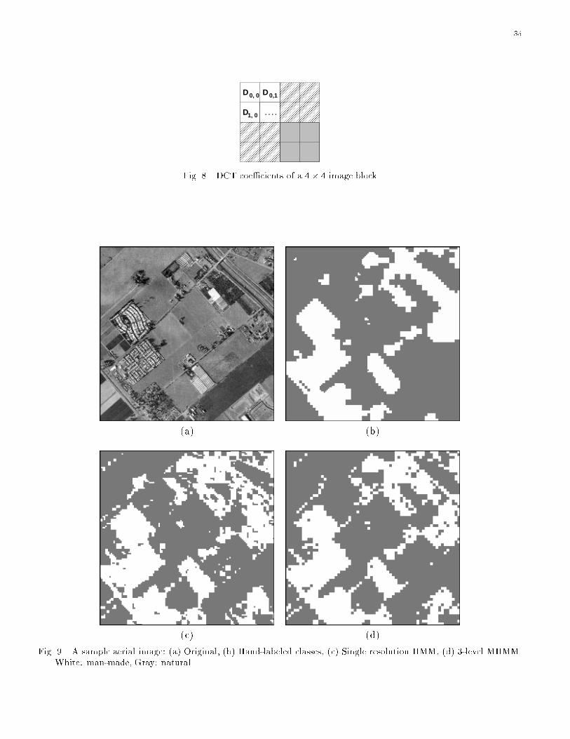
We applied our algorithm to the segmentation of man-made and natural regions of aerial images. The images

are 512� 512 gray-scale images with 8 bits per-pixel (bpp). They are aerial images of the San Francisco Bay

area provided by TRW (formerly ESL, Inc.) [30], [31]. An example of an image and its hand-labeled classi�ed

companion are shown in Figs. 9(a) and (b).

Feature vectors were extracted at three resolutions. Images at the two low resolutions were obtained by the

20

Daubechies 4 [12] wavelet transform. The images at Resolution 1 and 2 are, respectively, the LL bands of the

2-level and 1-level wavelet transforms. At each resolution, the image was divided into 4� 4 blocks, and DCT

coe�cients or averages over some of them were used as features. There are 6 such features. Denote the DCT

coe�cients for a 4� 4 block by fDi;j : i; j 2 (0; 1; 2; 3)g, shown by Fig. 8. The 6 features are de�ned as

1. f1 = D0;0 ; f2 = jD1;0j ; f3 = jD0;1j ;

2. f4 =P3

i=2

P1j=0 jDi;jj=4;

3. f5 =P1

i=0

P3j=2 jDi;jj=4 ;

4. f6 =P3

i=2

P3j=2 jDi;jj=4 .

DCT coe�cients at various frequencies re ect variation patterns in a block. They are more e�cient than

space domain pixel intensities for distinguishing classes. Alternative features based on frequency properties

include wavelet coe�cients.

In addition to the intra-block features computed from pixels within a block, the spatial derivatives of the

average intensity values of blocks were used as inter-block features. In particular, the spatial derivative

refers to the di�erence between the average intensity of a block and that of the block's upper neighbor or left

neighbor. The motivation for using inter-block features is similar to that for delta and acceleration coe�cients

in speech recognition [39], [25].

The MHMM algorithm and its two fast versions were tested by six-fold cross-validation [36], [6]. For each

iteration, one image was used as test data and the other �ve as training data. Performance is evaluated

by averaging over all iterations. Under a given computational complexity constraint, the number of states

in each class can be chosen according to the principle of Minimum Description Length [2]. The automatic

selection of those parameters has not been explored deeply in our current algorithm. Experiments, which will

be described, show that with a fairly small number of states, the MHMM algorithm outperforms the single

resolution HMM algorithm and other algorithms.

A 2-D MHMM tested is described by Table I(a), which lists the number of states assigned for each class

at each resolution. With the MHMM, the average classi�cation error rate computed at the �nest resolution

is 16:02%. To compare with well-known algorithms, we also used CARTR [6], a decision tree algorithm,

21

and LVQ1, version 1 of Kohonen's learning vector quantization algorithm [21], to segment the aerial images.

Classi�cation based on a single resolution HMM with 5 states for the natural class and 9 states for the man-

made class was also performed. All these algorithms were applied to feature vectors formed at the �nest

resolution in the same way as those used for the 2-D MHMM. Both the average classi�cation error rates and

the error rates for each testing image in the six-fold cross-validation are listed in Table II. It is shown that the

MHMM algorithm achieves lower error rates for all the testing images than the HMM algorithm, CART, and

LVQ1. On average, CART and LVQ1 perform about equally well. In [34], the Bayes VQ algorithm was used

to segment the aerial images. BVQ achieves an error rate of about 21:5%, nearly the same as that of CART.

The HMM algorithm improves CART and LVQ1 by roughly 13%. The MHMM algorithm further improves

the HMM by 15%.

The segmentation results for an example image are shown in Fig. 9(c) and (d). We see that the classi�ed

image based on the MHMM is both visually cleaner and closer to the hand-labeled classes in terms of clas-

si�cation error rates. The classi�cation error rate achieved by the MHMM for this image is 11:57%, whereas

the error rate for a single resolution HMM is 13:39%.

As is mentioned in Section III, some multiresolution models consider only inter-scale statistical dependence.

To test whether the intra-scale dependence assumed in the 2-D MHMM is redundant given the inter-scale

dependence, a 2-D MHMM discarding the intra-scale dependence was evaluated by six-fold cross-validation.

With this new model, given the state of a block, the states of its child blocks are independent. The number

of states assigned to each class at each resolution in the new 2-D MHMM as well as all the other parameters

controlling the computational complexity of the algorithm are the same as those used for the previous MHMM.

The average error rate achieved by the new model is 17:26%, whereas the average error rate with the previous

model is 16:02%. The experiment thus has demonstrated that the intra-scale dependence makes improvement

on classi�cation in addition to the inter-scale dependence.

To compare with existing multiresolution models, consider the quadtree MSRF developed by Bouman and

Shapiro [7]. The quadtree model assumes that, at the �nest resolution, the probability density function

of every class is a Gaussian mixture, which is equivalent to an HMM with several states in one class each

22

corresponding to a component of the mixture [39]. At all the coarse resolutions, since features do not exist

and only the prior probabilities of classes are considered, each class can be viewed as one state. Consequently,

we examined a 2-D MHMM with parameters shown in Table I(b). As the quadtree model ignores intra-scale

dependence, the 2-D MHMM was trained with the intra-scale dependence dismissed. Such a 2-D MHMM has

the same underlying state process as the quadtree model. Since the MSRF assumes features observed only

at the �nest resolution, when applying the 2-D MHMM to classi�cation, we blocked the e�ect of features at

the two coarse resolutions and only used the prior probabilities of classes for computing the joint posteriori

probability of states. The classi�cation error rate obtained by cross-validation is 18:89%, higher than the

error rate obtained with the HMM. For this 2-D MHMM, when features at the coarse resolutions are used,

the error rate is reduced to 17:63%.

Although a more advanced MSRF, namely the pyramid graph model, is also explored in [7] for segmentation,

comparison is constrained to the quadtree model because equivalence cannot be established between the

pyramid graph model and a 2-D MHMM. The former assumes that the state of a block depends on the states

of blocks in a neighborhood at the next coarser scale, while the latter assumes dependence on the parent block

and the sibling blocks at the same scale.

Experiments were performed on a Pentium Pro 230MHz PC with a LINUX operating system. For both the

single resolution HMM and the MHMM, computational complexity depends on many parameters including

the number of states in a model and parameters that control the extent of approximation taken by the path-

constrained Viterbi algorithm. Instead of comparing computational time directly, we compare classi�cation

performance given roughly equal computational time. The average CPU time to classify a 512 � 512 aerial

image with the HMM described previously is 200 seconds. With a 2-D MHMM described in Table I(c) and

somewhat arbitrarily chosen parameters required by the path-constrained Viterbi algorithm, the average user

CPU time to classify one image is 192 seconds, slightly less than that with the HMM. The average classi�cation

error rate is 17:32%, 8% lower than the error rate achieved with the HMM. By using the more sophisticated

model given by Table I(a) and more computation, the error rate can be improved further to 16:02%. With

the HMM, however, applying more sophisticated models and more computation does not yield considerable

23

improvement in performance.

The average user CPU time to classify one aerial image is 0:2 second for Fast Algorithm 1 and 7:3 seconds for

Fast Algorithm 2, much faster than the previous algorithms based on HMMs and MHMMs. The computation

time of Fast Algorithm 1 is very close to that of CART, which is 0:16 second on average. In all cases, the

classi�cation time provided here does not include the common feature computation time, which is a few

seconds. In the case of Fast Algorithm 1, the feature computation is the primary computational cost.

VIII. Testing Models

Although good results are achieved by algorithms based on the HMMs and MHMMs, which intuitively

justify the models, in this section we examine the validity of the models for images more formally by testing

their goodness of �t. The main reason for proposing the models is to balance their accuracy and computational

complexity; that they are absolutely correct is not really an issue. The purpose of testing is thus more for

gaining insight into how improvements can be made rather than for arguing the literal truthfulness of the

models.

A. Test of Normality

A 2-D HMM assumes that given its state, a feature vector is Gaussian distributed. The parameters of the

Gaussian distribution depend on the state. In order to test the normality of feature vectors in a particular

state, the states of the entire data set are searched according to the MAP (maximum a posteriori) rule using

an estimated model. Feature vectors in each state are then collected as data to verify the assumption of

normality. The test was performed on the aerial image data set described in Section VII. The model used is

a single resolution hidden Markov model with 5 states for the natural class and 9 states for the man-made

class.

The test of normality is based on the well-known fact that a multivariate normal distribution with covariance

proportional to the identity is uniform in direction. No matter the covariance, its projection onto any direction

has a normal distribution. For a general Gaussian distribution, a translation followed by a linear transform

can generate a random vector with unit spherical normal distribution, perhaps in dimension lower than that

24

of the original data. This process is usually referred to as decorrelation, or whitening.

For each state of the model, the normality of feature vectors was tested. The data were decorrelated and

then projected onto a variety of directions. The normal probability plot [4] for every projection was drawn.

If a random variable follows the normal distribution, the plot should be roughly a straight line through the

origin with unit slope. The projection directions include individual components of the vector, the average of

all the components, di�erences between all pairs of components, and 7 random directions. Since the feature

vectors are 8 dimensional, 44 directions were tested in all. Limitations of space preclude showing all the plots

here. Therefore, details are shown for one state which is representative of the others.

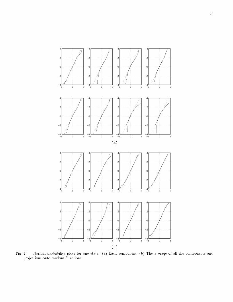
Fig. 10(a) is the normal probability plots for each of the 8 components. Counted row-wise, the 7th and 8th

plots in part (a) show typical \bad" �t to the normal distribution for projections onto individual components,

whereas the 1st plot is a typical \good" �t. \Bad" plots are characterized by data that are truncated below

and with heavy upper tails. Most plots resemble the 4th to 6th plots in part (a), which are slightly curved.

Fig. 10(b) shows plots for the average of all the components (the �rst plot) and projections onto random

directions. We see that the average and the projections onto the random directions �t better with the

normal distribution than do the individual components. These owe to a \central limit e�ect" and are shown

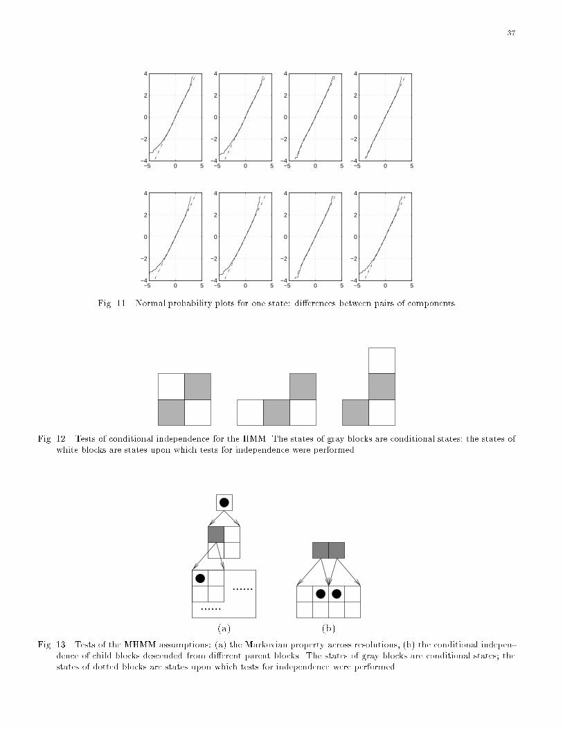
consistently by the other states. Fig. 11 presents the normal probability plots for di�erences between some

pairs of components. Di�erences between components also tend to �t normality better than the individual

components for all the states. A typical \good" �t is shown by the 3rd and the 7th plots, which are aligned

with the ideal straight line in a large range. A typical \bad" �t is shown by the 2nd and 6th plots, which only

deviate slightly from the straight line. But here, \bad" means heavy lower tails and truncated upper tails.

B. Test of the Markovian Assumption

For 2-D HMMs, it is assumed that given the states of the two neighboring blocks (right to the left and above),

the state of a block is conditionally independent of the other blocks in the \past." In particular, \past" means

all the blocks above and to the left. In this section, we test three cases of conditional independence given the

states of block (m;n) and (m�1; n+1): the independence of f(m�1; n); (m;n+1)g, f(m;n�1); (m;n+1)g,

25

and f(m;n+ 1); (m� 2; n + 1)g. For notational simplicity, we refer to the three cases as Cases 1, 2, and 3,

which are shown in Fig. 12.

For 2-D MHMMs, two assumptions are tested. One is the Markovian assumption that given the state of

a block at resolution r, the state of its parent block at resolution r � 1 and the states of its child blocks

at resolution r + 1 are independent. A special case investigated is the conditional independence of block

(i0; j0) 2 N(r�1) and one of its grandchild blocks (i2; j2), i2 = 4i0, j2 = 4j0, (i2; j2) 2 N

(r+1). Figure 13(a)

shows the conditioned and tested blocks. The other assumption tested is that given the states of parent blocks

at resolution r, the states of non-sibling blocks at resolution r + 1 are independent. In particular, a worst

possible case is discussed, that is, given the states of two adjacent blocks at resolution r, the states of their

two adjacent child blocks are independent. The spatial relation of those blocks is shown in Figure 13(b).

As with the test of normality in the previous section, the test of independence was performed on the aerial

image data set. States were searched by the MAP rule. Then, the test was performed on those states. In the

case of the HMM, the same model for the test of normality was used. For the MHMM, the 3 resolution model

described by Table I(c) was used.

To test the conditional independence, for each �xed pair of conditional states, a permutation �2 test [23], [8]

was applied. The idea of a permutation test dates back to Fisher's exact test [15] for independence in a 2� 2

contingency table [4]. In principle, Fisher's exact test can be generalized to testing independence of an r � c

contingency table. The di�culty is with computational complexity, which seriously constrains the use of exact

tests. Mehta and Patel [27] have taken a network approach to achieve computational feasibility. Boyett [8]

proposed subsampling random permutations to reduce computation. The random permutation approach is

taken here for simplicity.

Suppose the test for independence is for block (m� 1; n) and (m;n+ 1) (Case 1 of the HMM). The entry

�i;j in the contingency table is the number of occurrences for (m� 1; n) being in state i and (m;n+ 1) being

26

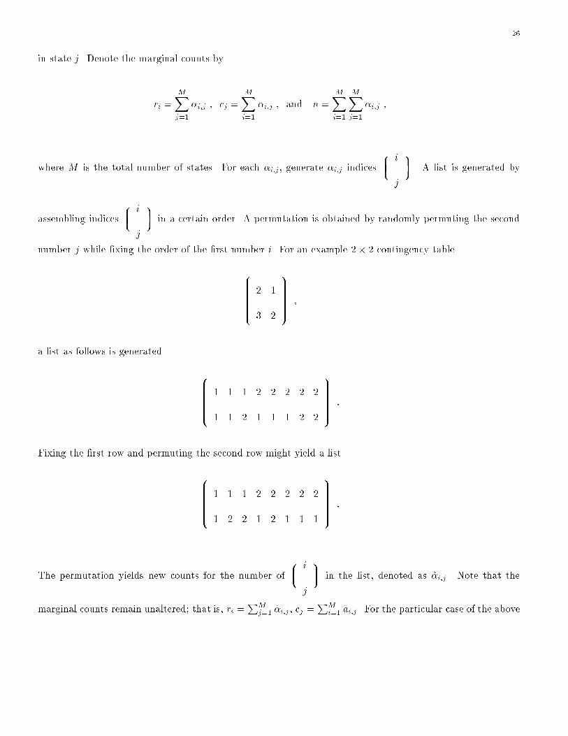
in state j. Denote the marginal counts by

ri =MXj=1

�i;j ; cj =MXi=1

�i;j ; and n =MXi=1

MXj=1

�i;j ;

where M is the total number of states. For each �i;j , generate �i;j indices

8>>: i

j

9>>;. A list is generated by

assembling indices

8>>: i

j

9>>; in a certain order. A permutation is obtained by randomly permuting the second

number j while �xing the order of the �rst number i. For an example 2� 2 contingency table

8>>>>>>>>>>:2 1

3 2

9>>>>>>>>>>;;

a list as follows is generated

8>>>>>>>>>>:1 1 1 2 2 2 2 2

1 1 2 1 1 1 2 2

9>>>>>>>>>>;:

Fixing the �rst row and permuting the second row might yield a list

8>>>>>>>>>>:1 1 1 2 2 2 2 2

1 2 2 1 2 1 1 1

9>>>>>>>>>>;:

The permutation yields new counts for the number of

8>>: i

j

9>>; in the list, denoted as �i;j . Note that the

marginal counts remain unaltered; that is, ri =PM

j=1 �i;j , cj =PM

i=1 ai;j . For the particular case of the above

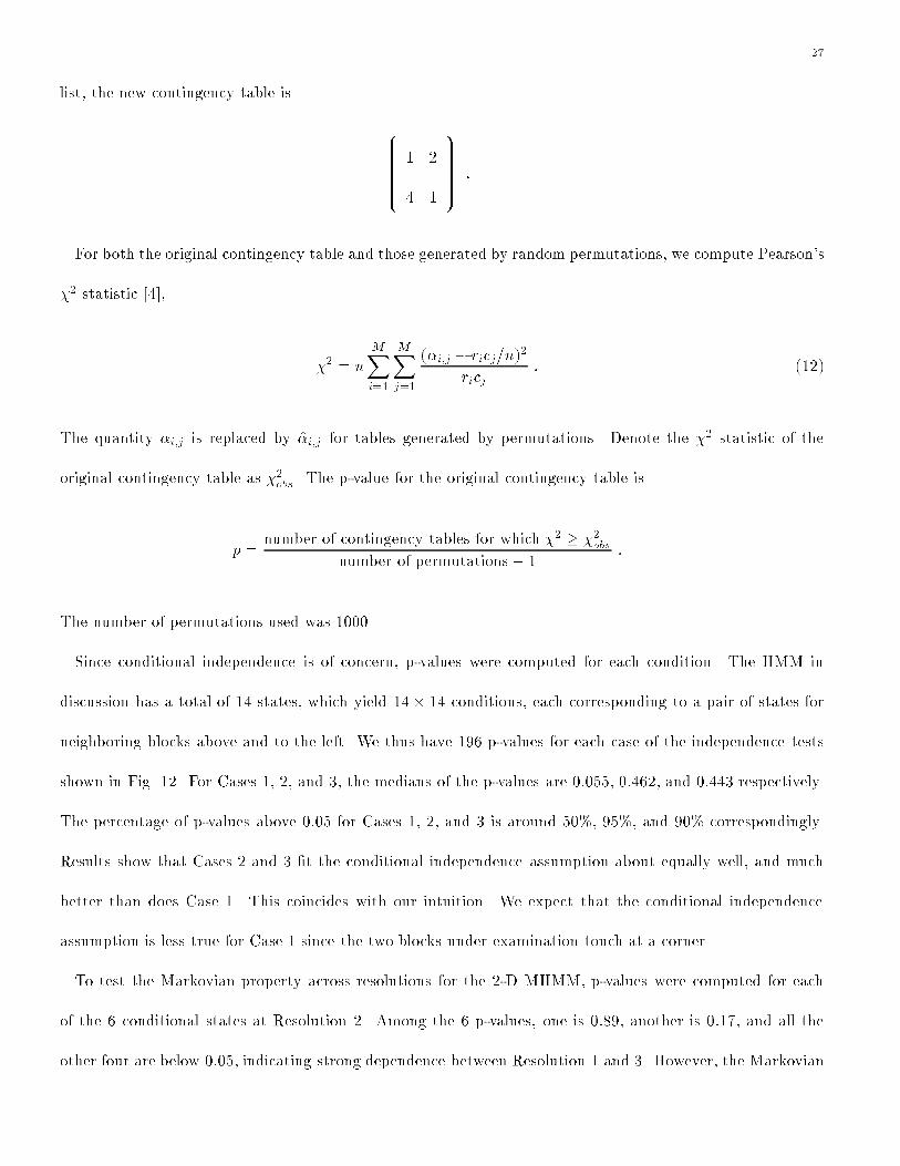
27

list, the new contingency table is

8>>>>>>>>>>:1 2

4 1

9>>>>>>>>>>;:

For both the original contingency table and those generated by random permutations, we compute Pearson's

�2 statistic [4],

�2 = n

MXi=1

MXj=1

(�i;j � ricj=n)2

ricj: (12)

The quantity �i;j is replaced by �i;j for tables generated by permutations. Denote the �2 statistic of the

original contingency table as �2obs. The p-value for the original contingency table is

p =number of contingency tables for which �2 � �2obs

number of permutations + 1:

The number of permutations used was 1000.

Since conditional independence is of concern, p-values were computed for each condition. The HMM in

discussion has a total of 14 states, which yield 14� 14 conditions, each corresponding to a pair of states for

neighboring blocks above and to the left. We thus have 196 p-values for each case of the independence tests

shown in Fig. 12. For Cases 1, 2, and 3, the medians of the p-values are 0:055, 0:462, and 0:443 respectively.

The percentage of p-values above 0:05 for Cases 1, 2, and 3 is around 50%, 95%, and 90% correspondingly.

Results show that Cases 2 and 3 �t the conditional independence assumption about equally well, and much

better than does Case 1. This coincides with our intuition. We expect that the conditional independence

assumption is less true for Case 1 since the two blocks under examination touch at a corner.

To test the Markovian property across resolutions for the 2-D MHMM, p-values were computed for each

of the 6 conditional states at Resolution 2. Among the 6 p-values, one is 0:89, another is 0:17, and all the

other four are below 0:05, indicating strong dependence between Resolution 1 and 3. However, the Markovian

28

property across resolutions is usually assumed to maintain computational tractability. For the testing of

conditional independence of non-sibling blocks, there are 6�6 = 36 state pairs of parent blocks, each of which

is a condition. The median of the 36 p-values is 0:44. About 70% of them are above 0:05. Therefore, for most

conditions, there is no strong evidence for dependence between blocks descended from di�erent parents.

IX. Conclusions

In this paper, a multiresolution 2-D hidden Markov model is proposed for image classi�cation, which rep-

resents images by feature vectors at several resolutions. At any particular resolution, the feature vectors are

statistically dependent through an underlying Markov mesh state process, similar to the assumptions of a

2-D HMM. The feature vectors are also statistically dependent across resolutions according to a hierarchical

structure. The application to aerial images showed results superior to those of the algorithm based on single

resolution HMMs. As the hierarchical structure of the multiresolution model is naturally suited to progressive

classi�cation if we relax the MAP rule, suboptimal fast algorithms were developed by searching for states in

a layered fashion instead of the joint optimization.

As classi�cation performance depends on the extent to which 2-D multiresolution hidden Markov models

apply, the model assumptions were tested. First, we tested, at least informally, the assumption that feature

vectors are Gaussian distributed given states. Normal probability plots show that the Gaussian assumption

is quite accurate. Second, we tested the Markovian properties of states across resolutions and within a

resolution. A permutation �2 test was used to test the conditional independence of states. The results do

not strongly support the Markovian property across resolutions, but this assumption is usually needed to

maintain computational tractability. At a �xed resolution, the bias of the Markovian property assumed by

the HMM is primarily due to assuming the conditional independence of a state and its neighboring state at

the left upper corner given the left and above neighboring states. Therefore, to improve a 2-D HMM, future

work should include the left upper neighbor in the conditioned states of transition probabilities.

Acknowledgments

The authors acknowledge the helpful suggestions of the reviewers.

29

References

[1] K. Abend, T. J. Harley, and L. N. Kanal, \Classi�cation of binary random patterns," IEEE Trans. Inform. Theory, vol.

IT-11, pp. 538-44, Oct. 1965.

[2] A. Barron, J. Rissanen, and B. Yu, \The minimum description length principle in coding and modeling," IEEE Transactions

on Information Theory, vol. 44, no. 6, pp. 2743-60, Oct. 1998.

[3] M. Basseville, A. Benveniste, K. C. Chou, S. A. Golden, R. Nikoukhah, and A. S. Willsky, \Modeling and estimation of

multiresolution stochastic processes," IEEE Trans. Inform. Theory, vol. 38, no. 2, pp. 766-784, March 1992.

[4] P. J. Bickel and K. A. Doksum, Mathematical Statistics: Basic Ideas and Selected Topics, Prentice Hall, Englewood Cli�s,

NJ, 1977.

[5] T. Binford, T. Levitt, and W. Mann, \Bayesian inference in model-based machine vision," Uncertainty in Arti�cial Intelli-

gence, J. F. Lemmer and L. M. Kanal, editors, Elsevier Science, 1988.

[6] L. Breiman, J. H. Friedman, R. A. Olshen, and C. J. Stone, Classi�cation and Regression Trees, Chapman & Hall, 1984.

[7] C. A. Bouman and M. Shapiro, \A multiscale random �eld model for Bayesian image segmentation," IEEE Trans. Image

Processing, vol. 3, no. 2, pp. 162-177, March 1994.

[8] J. M. Boyett, \Random RxC tables with given row and column totals," Applied Statistics, vol. 28, pp. 329-332, 1979.

[9] H. Choi and R. G. Baraniuk, \Image segmentation using wavelet-domain classi�cation," Proc. SPIE Technical Conference

on Mathematical Modeling, Bayesian Estimation, and Inverse Problems, pp. 306-320, July 1999.

[10] G. F. Cooper, \The computational complexity of probabilistic inference using Bayesian belief networks," Arti�cial Intelligence,

vol. 42, pp. 393-405, 1990.

[11] M. S. Crouse, R. D. Nowak, and R. G. Baraniuk, \Wavelet-based statistical signal processing using hidden Markov models,"

IEEE Trans. Signal Processing, vol. 46, no. 4, pp. 886-902, April 1998.

[12] I. Daubechies, Ten Lectures on Wavelets, Capital City Press, 1992.

[13] A. P. Dempster, N. M. Laird, and D. B. Rubin, \Maximum likelihood from incomplete data via the EM algorithm," Journal

Royal Statistics Society, vol. 39, no. 1, pp. 1-21, 1977.

[14] P. A. Devijver, \Probabilistic labeling in a hidden second order Markov mesh," Pattern Recognition in Practice II, pp. 113-23,

Amsterdam, Holland, 1985.

[15] R. A. Fisher, The Design of Experiments, Edinburgh, Oliver and Boyd, 1953.

[16] C. H. Fosgate, H. Krim, W. W. Irving, W. C. Karl, and A. S. Willsky, \Multiscale segmentation and anomaly enhancement

of SAR imagery," IEEE Trans. Image Processing, vol. 6, no. 1, pp. 7-20, Jan. 1997.

[17] W. T. Freeman and E. C. Pasztor, \Learning low-level vision," Proc. 7th Int. Conf. Computer Vision, Corfu, Greece, Sept.

1999.

30

[18] R. G. Gallager, Information Theory and Reliable Communication, John Wiley & Sons, Inc., 1968.

[19] D. Heckerman, \A tutorial on learning with Bayesian Networks," Microsoft Research Technical Report MSR-TR-95-06, Nov.

1996.

[20] D. Knill and W. Richards, editors, Perception as Bayesian Inference, Cambridge University Press, 1996.

[21] T. Kohonen, Self-Organization and Associative Memory, Springer-Verlag, Berlin, 1989.

[22] M. S. Landy and J. A. Movshon, editors, Computational Models of Visual Processing, MIT Press, Cambridge, MA, 1991.

[23] L. C. Lazzeroni and K. Lange, \Markov chains for Monte Carlo tests of genetic equilibrium in multidimensional contingency

tables," Annals of Statistics, vol. 25, pp. 138-168, 1997.

[24] E. Levin and R. Pieraccini, \Dynamic planar warping for optical character recognition," Int. Conf. Acoust., Speech and Signal

Processing, vol. 3, pp. 149-52, San Francisco, CA, March 1992.

[25] J. Li, A. Najmi, and R. M. Gray, \Image classi�cation by a two dimensional hidden Markov model," IEEE Trans. Signal

Processing, vol. 48, no. 2, pp. 517-33, February 2000.

[26] G. Loum, P. Provent, J. Lemoine, and E. Petit, \A new method for texture classi�cation based on wavelet transform," Proc.

3rd Int. Symp. Time-Frequency and Time-Scale Analysis, pp. 29-32, June 1996.

[27] C. R. Mehta and N. R. Patel, \A network algorithm for performing Fisher's exact test in r� c contingency tables," Journal

of the American Statistical Association, June 1983.

[28] Y. Meyer, Wavelets Algorithms and Applications, SIAM, Philadelphia, 1993.

[29] R. D. Nowak, \Multiscale hidden Markov models for Bayesian image analysis," Bayesian Inference in Wavelet Based Models,

pp. 243-266, Springer-Verlag, 1999.

[30] K. L. Oehler, \Image compression and classi�cation using vector quantization," Ph.D thesis, Stanford University, 1993.

[31] K. L. Oehler and R. M. Gray, \Combining image compression and classi�cation using vector quantization," IEEE Trans. on

Pattern Analysis and Machine Intelligence, vol. 17, no. 5, pp. 461-73, May 1995.

[32] J. Pearl, Probabilistic Reasoning in Intelligent Systems: Networks of Plausible Inference, Morgan Kaufmann, 1988.

[33] P. P�erez and F. Heitz, \Restriction of a Markov random �eld on a graph and multiresolution statistical image modeling,"

IEEE Trans. Inform. Theory, vol. 42, no. 1, pp. 180-90, Jan. 1996.

[34] K. O. Perlmutter, S. M. Perlmutter, R. M. Gray, R. A. Olshen, and K. L. Oehler, \Bayes risk weighted vector quantization

with posterior estimation for image compression and classi�cation," IEEE Trans. Image Processing, vol. 5, no. 2, pp. 347-60,

Feb. 1996.

[35] C. E. Shannon, \A mathematical theory of communication," Bell System Technical Journal, vol. 27, pp. 379-423, July 1948.

[36] M. Stone, \Cross-validation: a review," Math. Operationforsch. Statist. Ser. Statist., no. 9, pp. 127-39, 1978.

[37] M. Unser, \Texture classi�cation and segmentation using wavelet frames," IEEE Trans. Image Processing, vol. 4, no. 11, pp.

1549-60, Nov. 1995.

31

[38] A. J. Viterbi and J. K. Omura, \Trellis encoding of memoryless discrete-time sources with a �delity criterion," IEEE Trans.

Inform. Theory, vol. IT-20, pp. 325-32, May 1974.

[39] S. Young, J. Jansen, J. Odell, D. Ollason, and P. Woodland, HTK - Hidden Markov Model Toolkit, Cambridge University,

1995.

32

Class res 1 res 2 res 3

natural 5 5 5

man-made 5 5 9

mixed 4 2 0

(a)

Class res 1 res 2 res 3

natural 1 1 5

man-made 1 1 9

mixed 1 1 0

Class res 1 res 2 res 3

natural 2 2 5

man-made 2 2 9

mixed 2 2 0

(b) (c)

TABLE I

The number of states for each class at each resolution

Iteration CART LVQ1 HMM MHMM Fast 1 Fast 2

1 0.2263 0.2161 0.1904 0.1733 0.1886 0.1855

2 0.1803 0.1918 0.1765 0.1636 0.1566 0.1392

3 0.2899 0.2846 0.2034 0.1782 0.2914 0.2857

4 0.2529 0.2492 0.2405 0.2051 0.2430 0.2277

5 0.1425 0.1868 0.1834 0.1255 0.1906 0.1541

6 0.2029 0.1813 0.1339 0.1157 0.1816 0.1766

Ave. 0.2158 0.2183 0.1880 0.1602 0.2086 0.1948

TABLE II

Classification error rates at the finest resolution by different algorithms

(a) (b) (c)

Fig. 1. The segmentation process of the human vision system: (a) Original image, (b) A rough segmentation with thegray region being undecided, (c) The re�ned segmentation

33

(1)i, jx

(2)i, jx i, j

(3)x

Fig. 2. Multiple resolutions of an image

Childblocks

Parentblock

������

������

������

������������������������

������

Fig. 3. The image hierarchy across resolutions

Resolution 2

Resolution 3

Resolution 1

������������������������

������������������������

������������������������

������������������������

������������������������

������������������������

������������������������

��������������������������������������������������������������������������������������������������������

��������������������������������������������������������������������������������

����������������������������������������

����������������������������������������

������

������

���

���

���

���

������

������

������

������

������

������

������

������

������

������

���

���

��������

������

������

������

������

��������

��������

��������

��������

��������

��������

��������

��������

����

������

������

������������������������������������������������������������������������������������������������������������������������������������������������������������������������������������������������������������������������������������������������������������������������������������������������������������������������������������������������������������������������������������������������������������������������������������������������������������������������������������

������������������������������������������������������������������������������������������������������������������������������������������������������������������������������������������������������������������������������������������������������������������������������������������������������������������������������������������������������������������������������������������������������������������������������������������������������������������������������������

�����������������������������������������������������������������������������������������������������������������������������

�����������������������������������������������������������������������������������������������������������������������������

������������������������������������

������������������������������������

���������������

���������������

���������������

���������������

������������������������������������������������

������������������������������������������������

��������������������������������

��������������������������������

����������������������������������������������������������������������������������������������������

����������������������������������������������������������������������������������������������������

��������������������������������������������

��������������������������������������������

���������������������������������

���������������������������������

����������������

����������������

������������������������������������������������������������������������������������������������

������������������������������������������������������������������������������������������������

��������

��������

������

������

������

������

�������������������������������������������������������������������������������������������������������������������������������������������������������������������������������

�������������������������������������������������������������������������������������������������������������������������������������������������������������������������������

��������������������������������������������������������������������������������

��������������������������������������������������������������������������������

��������������������������������

��������������������������������

������

������

������

������

����

Fig. 4. The hierarchical statistical dependence across resolutions

34

(a) (b) (c)

Fig. 5. Three possible structures of MHMMs on an 8 � 8 grid of blocks: (a) a 3-level MHMM with quadtree splitand the coarsest resolution modeled by an HMM on a 2� 2 grid, (b) a 2-level MHMM with quadtree split and thecoarsest resolution modeled by an HMM on a 4 � 4 grid, (c) a 2-level MHMM with 4 � 4 split and the coarsestresolution modeled by an HMM on a 2� 2 grid.

T0

T1

. .

.

. . . . . T

T T

w-1

w w+z-2

Fig. 6. Blocks on the diagonals of an image

��������

��������

����

����

����

��������

����

����

��������

��������

����

���������

���������

���������

���������

1

2

3

4 5����

����

������ ��

���� ���� ��

2-D Viterbi state transition

1

2

3

4

5

position

SequencesState

Fig. 7. The variable-state Viterbi algorithm

35

������������������������������������

������������������������������������������

������������������������������

������������������������������������

D1, 0

D 0,1D 0, 0

. . . .

Fig. 8. DCT coe�cients of a 4� 4 image block

(a) (b)

(c) (d)

Fig. 9. A sample aerial image: (a) Original, (b) Hand-labeled classes, (c) Single resolution HMM, (d) 3-level MHMM.White: man-made, Gray: natural

36

−5 0 5−4

−2

0

2

4

−5 0 5−4

−2

0

2

4

−5 0 5−4

−2

0

2

4

−5 0 5−4

−2

0

2

4

−5 0 5−4

−2

0

2

4

−5 0 5−4

−2

0

2

4

−5 0 5−4

−2

0

2

4

−5 0 5−4

−2

0

2

4

(a)

−5 0 5−4

−2

0

2

4

−5 0 5−4

−2

0

2

4

−5 0 5−4

−2

0

2

4

−5 0 5−4

−2

0

2

4

−5 0 5−4

−2

0

2

4

−5 0 5−4

−2

0

2

4

−5 0 5−4

−2

0

2

4

−5 0 5−4

−2

0

2

4

(b)

Fig. 10. Normal probability plots for one state: (a) Each component, (b) The average of all the components andprojections onto random directions

37

−5 0 5−4

−2

0

2

4

−5 0 5−4

−2

0

2

4

−5 0 5−4

−2

0

2

4

−5 0 5−4

−2

0

2

4

−5 0 5−4

−2

0

2

4

−5 0 5−4

−2

0

2

4

−5 0 5−4

−2

0

2

4

−5 0 5−4

−2

0

2

4

Fig. 11. Normal probability plots for one state: di�erences between pairs of components

Fig. 12. Tests of conditional independence for the HMM. The states of gray blocks are conditional states; the states ofwhite blocks are states upon which tests for independence were performed.

......

......

(a) (b)

Fig. 13. Tests of the MHMM assumptions: (a) the Markovian property across resolutions, (b) the conditional indepen-dence of child blocks descended from di�erent parent blocks. The states of gray blocks are conditional states; thestates of dotted blocks are states upon which tests for independence were performed.