Multiscale Decision-Making for Multiple Decision … Singh for her detailed account of hospital organizational environments, which impacted my thesis significantly

Multiscale Decision-Making for Multiple Decision Alternatives

Swathi Priyadarshini Sudhaakar

Thesis submitted to the faculty of the Virginia Polytechnic Institute and State

University in partial fulfillment of the requirements for the degree of

Master of Science

in

Industrial and Systems Engineering

Christian L. Wernz

Ebru K. Bish

Michael R. Taaffe

12/10/2012

Blacksburg, Virginia

Keywords: Multiscale Decision-Making, Decision Analysis, Optimal Incentives,

Hierarchical Agents, Health Care Decision Support

Multiscale Decision-Making for Multiple Decision Alternatives

Swathi Sudhaakar

ABSTRACT

In organizations with decision makers across multiple hierarchical levels, conflicting

objectives are commonly observed. The decision maker, or agent, at the highest level usually

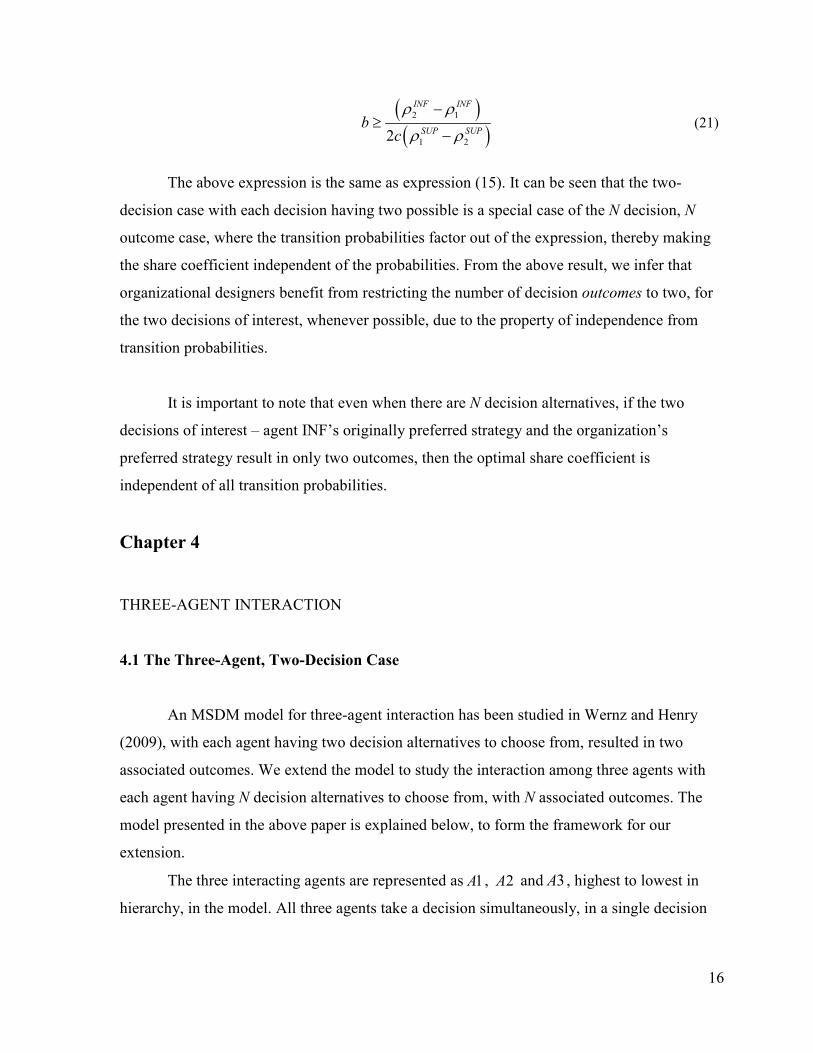
makes decisions in the interest of the organization, while a subordinate agent may have a

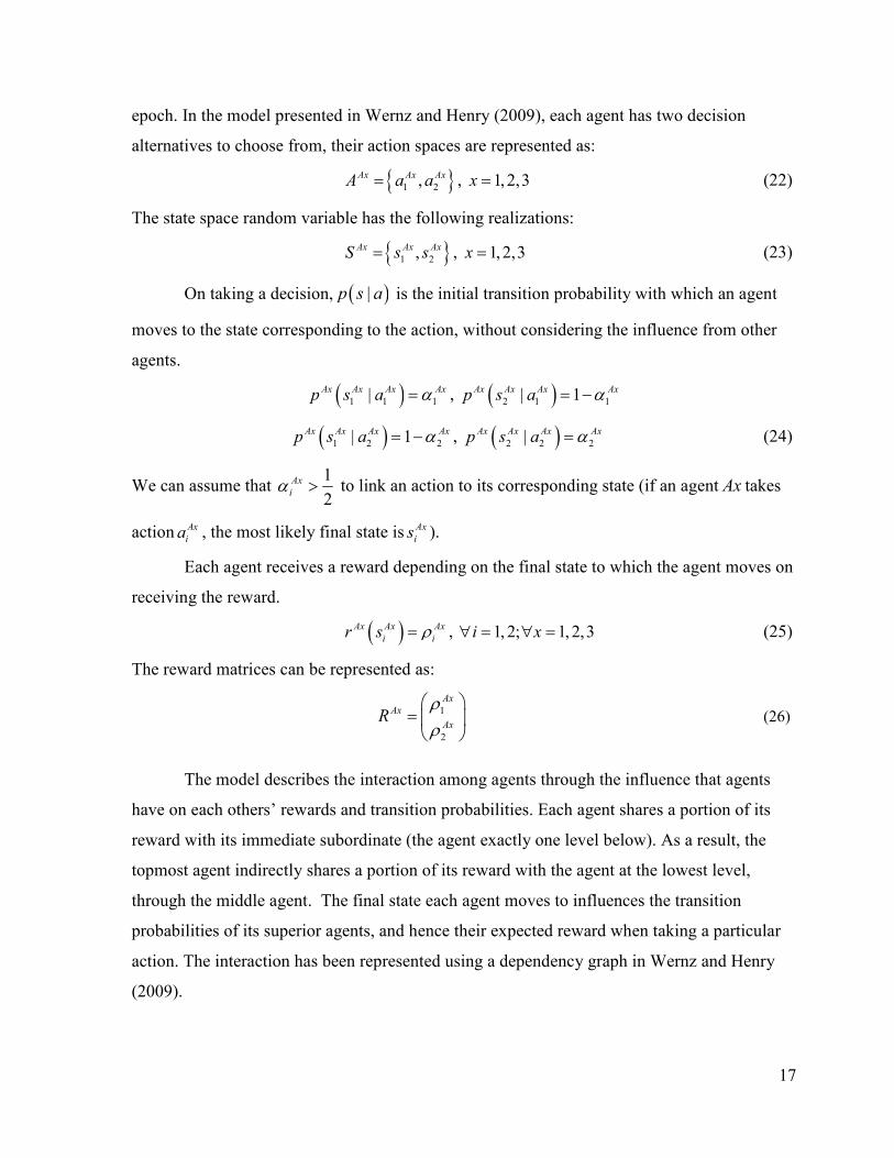
conflict of interest between taking a course of action that is best for the organization and the

course of action that is best for itself.

The Multiscale Decision-Making (MSDM) model was established by Wernz (2008).

The model has been developed to capture interactions in multi-agent systems, by integrating

both the hierarchical and temporal scale of decisions made in organizations.

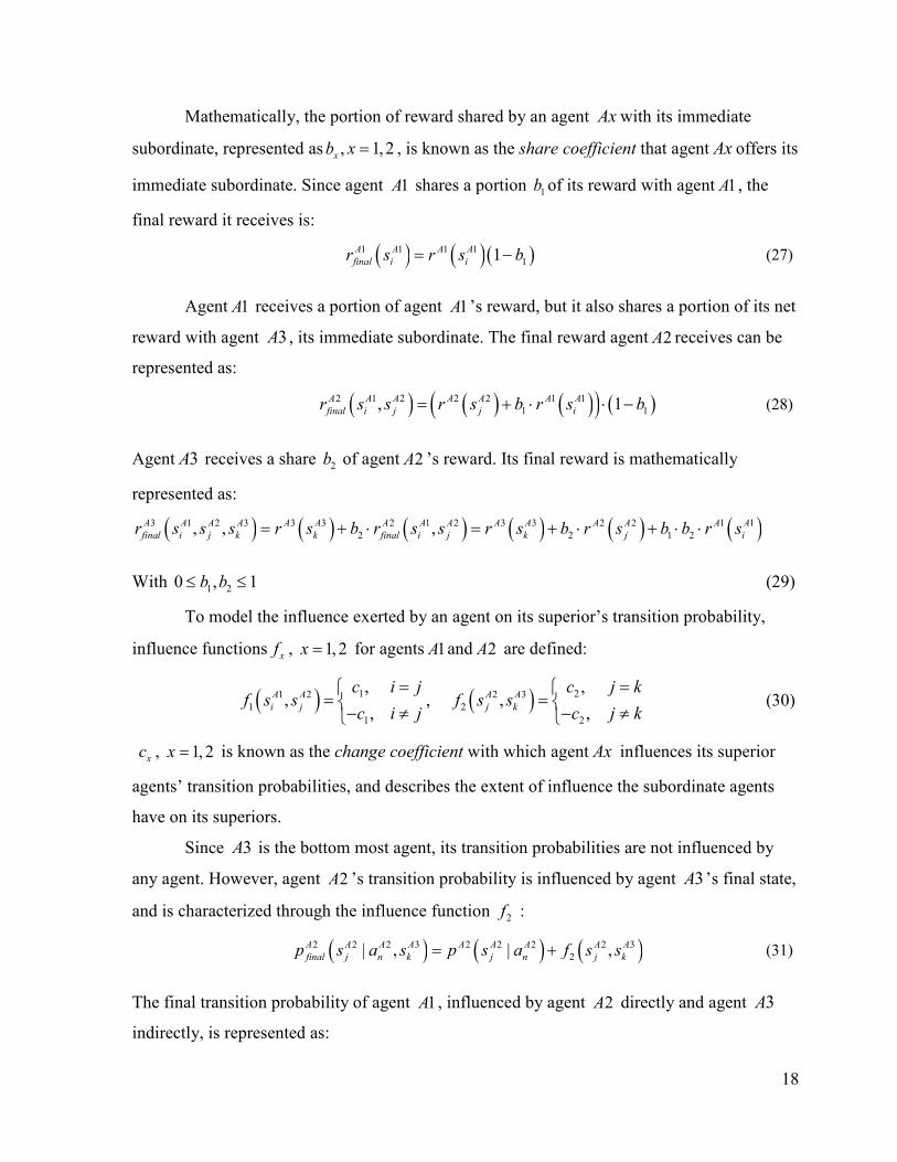
This thesis contributes towards expanding the results in the hierarchical interaction

domain of MSDM by extending the model to incorporate N decision alternatives and

outcomes instead of two, and studying its effect on the interaction between agents.

We consider decisions with uncertain outcomes, where the outcomes of the decisions

made by agents lower in hierarchy affect the transition probabilities of the decisions made by

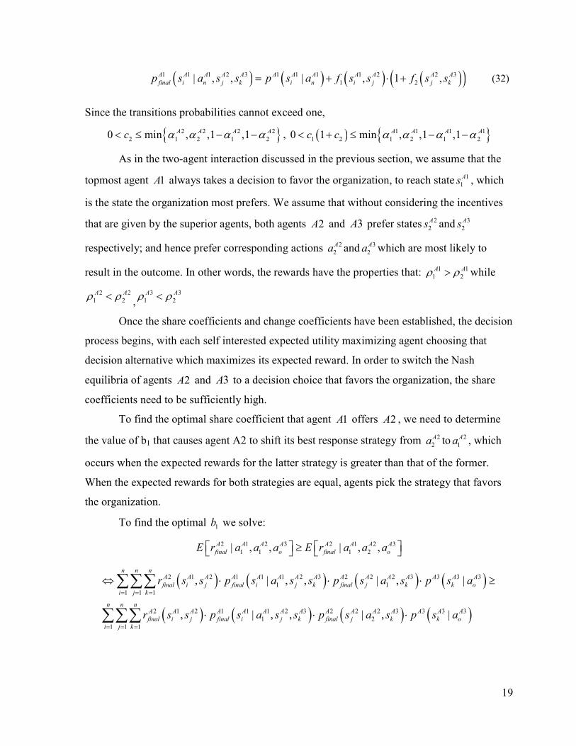
agents above them in hierarchy. This leads to a game theoretic situation, where the lower-level

agents need to be sufficiently incentivized in order to shift their best response strategy to one

in the interest of their superior and the organization. Mathematical expressions for the optimal

incentives at each hierarchical level are developed.

We analyze systems with agents interacting across two and three organizational levels.

We then study the effect of introducing the cost of taking an action on the optimal incentives.

We discuss a health care application of MSDM.

iii

To my family...

ACKNOWLEDGMENTS

I would like to thank my advisor, Dr.Christian Wernz, for the opportunity to pursue

research under his guidance. I thank him for the financial support and encouragement he

provided me. The freedom he gave me helped me explore and get deeply involved with my

area of study. His relentless effort in helping me shape my thoughts and research style has

taught me some very valuable lessons. I would like to thank my committee members Dr.Ebru

Bish and Dr.Michael Taaffe for their invaluable insights and perspectives that helped me

improve my work. I also thank the Grado Department of Industrial and Systems Engineering

and the Physics Department at Virginia Tech for giving me the resources that enabled me to

pursue my education.

I thank my family and friends for their love, support and guidance throughout all my

endeavors. I thank my brother, Dr.Raghuram Sudhaakar, for guiding me through graduate

school and helping me learn from his experiences. I thank Rohit Kota for being a bouncing

board for my thoughts and ideas. I thank Daniel Steeneck for his feedback and insights, and

Dr.Urvashi Singh for her detailed account of hospital organizational environments, which

impacted my thesis significantly. I can’t thank my parents enough for their hard work and

dedication in ensuring I received quality education. They made it all worth it, and this

wouldn’t have been possible without them.

Table of Contents Page

Chapter 1. INTRODUCTION ..............................................................................................1

1.2 Motivation ................................................................................................................1

1.2 Overview ..................................................................................................................1

Chapter 2. RELATED WORK ............................................................................................2

Chapter 3. TWO-AGENT INTERACTION ........................................................................5

3.1 An Example .............................................................................................................5

3.2 The Two-Agent, Two-Decision Case ......................................................................8

3.3 The Two-Agent, N-Decision Case .........................................................................12

3.4 The Two-Decision Case - A Special Case of the N-Decision Case .......................15

Chapter 4. THREE-AGENT INTERACTION ..................................................................16

4.1 The Three-Agent, Two-Decision Case ..................................................................16

4.2 The Three-Agent, N-Decision Case .......................................................................20

4.3 The Two-Decision Case - A Special Case of the N-Decision Case .......................23

Chapter 5. TWO AND THREE-AGENT INTERACTION WITH COST OF ACTION..24

5.1 Cost of Action in the Two-Agent Interaction Model .............................................25

5.2 Cost of Action in the Three-Agent Interaction Model ...........................................25

Chapter 6. DISCUSSION, CONCLUSION AND FUTURE RESEARCH ......................26

6.1 Discussion ..............................................................................................................26

6.1.1 On the Change Coefficient............................................................................26

6.1.2 On the Share Coefficient ...............................................................................27

6.2 Conclusion .............................................................................................................27

6.3 Future Research .....................................................................................................28

REFERENCES ..................................................................................................................29

List of Figures

Figure 1: Hierarchy of Agents in a Hospital (Hallisy and Haskel 2009) .................................... 5

Figure 2: Agent interaction in the Health Check-up Scenario .................................................... 7

Figure 3: Timeline of Decisions made by Agents ...................................................................... 8

Figure 4: Indifference curve for Two-agent Interaction with two decision outcomes ............. 12

Figure 5: Graph that represents actions and associated outcomes ............................................ 15

Figure 6: Graphical Representation of Three-agent Interaction ............................................... 22

1

Chapter 1

INTRODUCTION

1.1 Motivation

In organizations with decision makers across multiple hierarchical levels, conflicting

objectives are commonly observed. The decision maker, or agent, at the highest level usually

makes decisions in the interest of the organization, while a subordinate agent may have a

conflict of interest between taking a course of action that is best for the organization and the

course of action that is best for itself.

The Multiscale Decision-Making (MSDM) model was established by Wernz (2008) .

The model describes a novel approach capturing interactions in multi-agent systems, by

integrating both the hierarchical and temporal scales of decisions made in organizations. The

model suggests a method to compute the optimal incentives that each agent should offer to its

subordinate to enable cooperation, taking into consideration two decision alternatives which

lead to one of two associated outcomes with uncertainty. The model and associated results for

the optimal incentive have been developed for two-agent interactions and three-agent

interactions, considering only two decision alternatives and outcomes. Existing work does not

address the effect of having more than two decision alternatives and outcomes for each agent.

In order to take the MSDM model towards real-world applications, a general model is

required, considering as many decision alternatives, outcomes and agents as the organization

contains. This work has generalized the number of decision alternatives and outcomes

available, contributing to the hierarchical section of MSDM, thereby making available general

two-agent and three-agent interaction models, which can be applied in real-world applications

discussed in the following chapters.

1.2 Overview

We begin with a review of the literature in Chapter 2, where an extensive review of

existing work in economics and decision theory is presented. In Chapter 3, the model is

motivated with an example in health care decision-making in a hierarchical hospital

environment. We describe briefly the agents, interactions and the decisions made by each

2

agent. Following the example, we introduce the MSDM model with two agents and two

decision alternatives and outcomes and proceed to explain the general N-decision outcome

model. We then discuss the two-decision outcome case as a special case of the general model,

and discuss the optimal incentives in the different cases.

In Chapter 4, we introduce the three-agent model with N decision outcomes, and we

study how the optimal incentives behave in this model. In Chapter 5, we present a variation of

the model described, by introducing the cost of action for each decision, and we study the

effect on the optimal incentive expressions. In Chapter 6, a discussion that gives insights to

organizational designers on measuring organizational parameters relevant to the model is

presented, and future research potential is discussed in conclusion.

Chapter 2

RELATED WORK

Since the aim of this work is to contribute to the hierarchical section of Multiscale

Decision-Making, a survey of hierarchical decision-making literature is presented below.

A classification of hierarchical agent interactions is presented by Schneeweiss (2003) where

constructional and organizational systems are defined as the primary classes of distributed

decision- making. Constructional systems refer to those with only one decision maker at each

level, where information symmetry prevails. Organizational systems, in contrast, are

characterized by information asymmetry with decision makers in leadership roles, including

time-based decision hierarchies such as operational and tactical decisions.

From an economics perspective, Williamson (1967) proposed a mathematical model to

identify the optimal number of hierarchical levels in an organization. The input parameters

include the number of employees a supervisor can handle effectively (span of control),

fraction of work done by a subordinate that contributes to the objectives of the superior

(compliance parameter), wage of employees at each level, among others, and the dependency

of the optimal number of hierarchical levels on these parameters are discussed. While the

author discussed structuring organizations, quantitative methods to improve degree of

3

compliance among hierarchical levels are not dealt with. Organizational hierarchy is modeled

by Prat (1997) and Qian (1994).

Harris, Kriebel et al. (1982) discussed intra-firm resource allocation among various

division managers. The authors developed a model that makes a trade-off between

information asymmetry at different levels, and potential conflict of objective between higher-

level and lower-level decision makers, to suggest an optimal resource allocation among

departments in an organization. The authors, however, did not discuss how objectives can be

aligned, and incentives shared optimally within the departments, among hierarchies. Harris

and Raviv (2002) also discussed the cost minimal organizational design, among matrix

organizations, functional hierarchies, divisional hierarchies or flat hierarchies, based on the

characteristics of activities and managerial costs of agents.

Vroom (2006) studied the interaction between remuneration structures in an

organization and competitiveness of the organization, concluding that similar organizational

structures promote increased rivalry among firms. Fershtman and Judd (1987), in their

seminal paper on economic incentives in an owner-manager organization facing competition

from another similar firm, discussed a two-stage game. In the first stage, the owners offered

an incentive contract to the managers in the presence of demand uncertainty. In the second

stage, the managers had full information about the realized demand as well as the incentive

contracts of the managers of the other firm, and they played an oligopoly game to maximize

their expected profit. The authors did not discuss a scenario when both the owner and

manager have to act simultaneously under outcome uncertainty. The authors view the owner’s

role as only that of offering an incentive contract, and did not discuss the interaction between

the owner and manager when the owner makes organizational decisions whose outcome is

affected by the manager’s actions. Knott (2001) compared hierarchy in organizations to

market design and its impact on organizational performance.

Deng and Papadimitriou (1999) discussed hierarchical decision-making scenarios in

organizations, where conflicting objectives exist between agents at different hierarchies. The

authors suggested a mathematical programming approach to decision-making, where each

rational agent intends to maximize its own objective function. The agents engage in game-

theoretic reasoning process, where the top-most agent moves first, and the other agents

follow, in choosing their strategies, which aligned with the most optimal Nash equilibrium of

4

the game. The authors derived a set of conditions for which the firm is considered efficient.

However, the authors did not consider stochastic decision outcomes, or attempt to provide

incentives at each stage to enable cooperation among agents.

Principal-agent theory models a range of problems with two hierarchically interacting

agents, with incomplete and asymmetric information. In Milgrom and Roberts (1992), an

overview of the principal-agent theory is given. The principal is the superior decision maker

who offers a contract to make the lower-level decision maker, known as the agent, which is

designed to motivate the agent to perform work in interest of the principal. The agent involves

in a game-theoretic reasoning process to select the option with the highest expected utility.

The MSDM model describes agent interaction that differs from the principal-agent

problem in the following critical ways: The superior agent does not hire the lower-level agent

as the organizational structure has been established by an external organizational designer.

Additionally, the superior agent cannot impose a penalty on the subordinate agent.

Holmstrom and Milgrom (1991) discussed why employment is better than contracting

using a linear principal-agent model developed in Holmstrom and Milgrom (1987). Grossman

and Hart (1983) discussed a model where the agent needs to solve a convex linear program to

find the optimal action. Rogerson (1985) compared the approaches of considering utility as a

stationary point as opposed to the first order solution of utility maximization, where the author

argues that the former is a better approach. Jewitt (1988), on the other hand, support the first

order solution to be the better approach.

To motivate the healthcare application, existing performance measures for physicians

in large hospitals were studied. Lanier, Roland et al. (2003) presented a comprehensive review

of existing initiatives to measure physician performance in the US, the UK and the

Netherlands.Werner and Bradlow (2006) discussed the relationship between the hospital

compare performance measures used by the CMS (Centers for Medicare and Medicaid

Services), and the risk adjusted mortality rates of hospitals. Chen, Yamauchi et al. (2006)

discussed the use of BSC (Balanced Scorecards) to measure the performance of hospitals in

Japan and China. The literature does not seem to address patient satisfaction as a performance

metric for physicians.

Chapter 3

TWO-AGENT INTERACTION

3.1 An Example

With the Patient Protection and Affordable Care Act (PPACA) being passed in March

2010, the compensation structure of payment to hospitals from the Center for Medica

Medicaid Services (CMS) has changed significantly. The PPACA has introduced the quality

of care provided to the patients as additional criteria

quantity of care. As a result, hospital profits are increasingly d

Patient satisfaction is impacted by the overall experience in the hospital, and hence

requires all the levels of employees in a hospital to work in unison towards ensuring that the

patient is satisfied. Hence, studying th

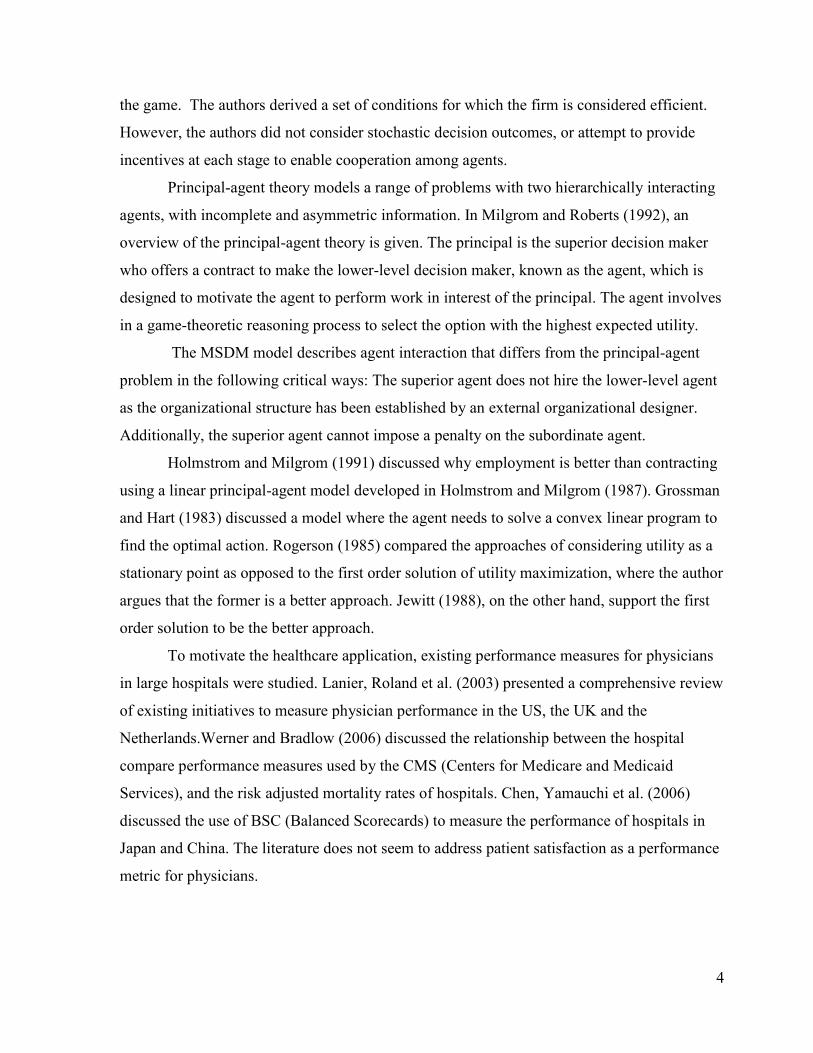
interactions between each level is required. D

structured as shown in Figure 1.

Figure 1: Hierarchy

The medical director is interested in improving the patient satisfaction levels for the

health check-up packages that the hospital offers, in order

program. Health check-up packages usually consist of a series of health screening tests,

which patients interact with the physicians and nurses to understand their current wellness,

AGENT INTERACTION


2010, the compensation structure of payment to hospitals from the Center for Medica


patients as additional criteria for reimbursement, instead of just the

quantity of care. As a result, hospital profits are increasingly dependent on patient satisfaction.



patient is satisfied. Hence, studying the various levels in a hospital hierarchy, and the

interactions between each level is required. Decision makers in hospitals are hierarchically

as shown in Figure 1.

: Hierarchy of Agents in a Hospital (Hallisy and Haskel 2009)

edical director is interested in improving the patient satisfaction levels for the

up packages that the hospital offers, in order to increase the profitability of the

up packages usually consist of a series of health screening tests,

with the physicians and nurses to understand their current wellness,

5


2010, the compensation structure of payment to hospitals from the Center for Medicare and


for reimbursement, instead of just the

endent on patient satisfaction.



e various levels in a hospital hierarchy, and the

are hierarchically

)

edical director is interested in improving the patient satisfaction levels for the

to increase the profitability of the

up packages usually consist of a series of health screening tests, during

with the physicians and nurses to understand their current wellness,

6

and measures to be taken to improve it. Each department head is allocated with the task of

setting up training and incentive programs to ensure that the end goal of improving patient

satisfaction is met. We consider the interaction between the head of the department and the

attending physician to motivate our two-agent model.

In order to improve the patient satisfaction and associated profits, the head of the

department decides to implement a nurse training program, with special focus on health

check-up related patient care. During the health check-up program, the attending physician

can decide to conduct an in-depth physical examination, spending more time per patient,

explaining in detail the various aspects of the patient’s health, or a quick physical

examination, spending lesser time and providing a superficial overview of the patient’s

wellness. The patient’s perception of satisfaction is affected by the experience with the

physician.

The performance of the physicians employed by the hospital is mainly evaluated by

their percent compliance to medical procedures, morbidity and mortality reviews and peer

reviews (Lanier, Roland et al. 2003). These measures take into consideration response to

inpatients which have higher medical and legal consequences, but do not cover their

performance in health check-up programs as the consequences are not as critical. A physician

is scheduled to conduct a fixed number of health check-ups in a day, irrespective of which

type of service the physician offers, as the actual service offered can be measured only when

the outcome of patient satisfaction levels has been realized. This eliminates the possibility of

making increased profits by offering the quicker service and increasing the volume of patients

per physician.

Physicians, who are not motivated purely by ensuring that their patients are satisfied,

may prefer to conduct a quick physical examination, as it most likely involves spending lesser

time with the patient. For the purpose of this example, we make the assumption that the

physicians considered seek to spend minimal time with patients. The probability that the head

of the department achieves his goal of improved patient satisfaction (profits) increases when

the physician chooses to conduct an in-depth physical examination. This leads to a conflict of

interest between the head of the department and the physician.

As a result, the head of the department is willing to share a portion of the additional

profits received as a consequence of high patient satisfaction with the physician, to motivate

the physician to switch to an initially less favorable action. One form of incentive offered

could be in the form of medical

existing rewards are not sufficient to motivate the physicians to behave in favor of the

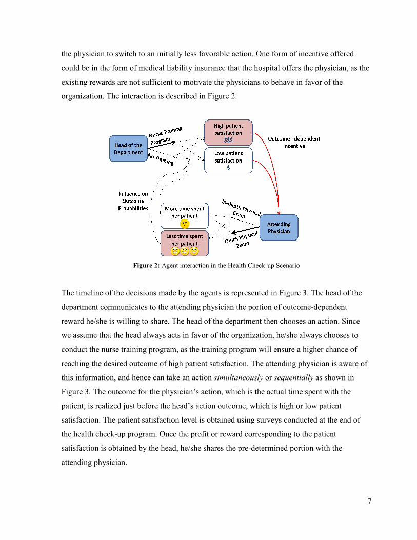
organization. The interaction is described in Figure 2.

Figure 2

The timeline of the decisions made

department communicates to the attending physician the port

reward he/she is willing to share. The head of the department then chooses an action. Since

we assume that the head always acts in favor of the organization, he/she always chooses to

conduct the nurse training program

reaching the desired outcome of high patient satisfaction

this information, and hence can take an action

Figure 3. The outcome for the physician’s action, which is the actual time spent with the

patient, is realized just before the head’s action outcome, which is high or

satisfaction. The patient satisfaction level is obtained using surveys conducted at the end of

the health check-up program. Once the profit or reward corresponding to the patient

satisfaction is obtained by the head, he/she shares the pre

attending physician.


medical liability insurance that the hospital offers the

rds are not sufficient to motivate the physicians to behave in favor of the

The interaction is described in Figure 2.

2: Agent interaction in the Health Check-up Scenario

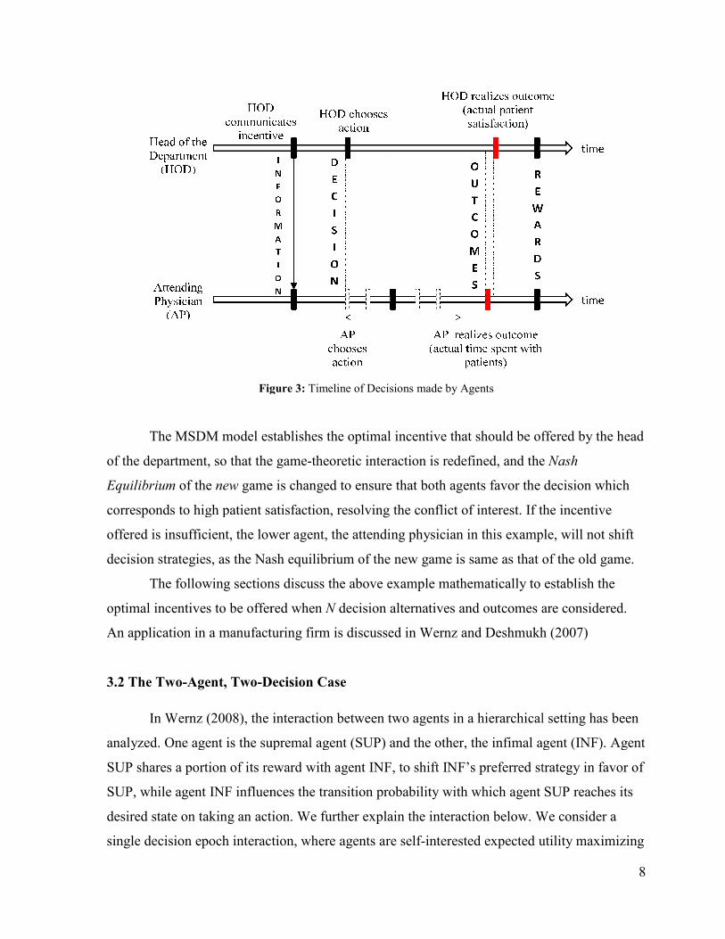
The timeline of the decisions made by the agents is represented in Figure 3. The head of the

department communicates to the attending physician the portion of outcome-


ad always acts in favor of the organization, he/she always chooses to

conduct the nurse training program, as the training program will ensure a higher chance of

reaching the desired outcome of high patient satisfaction. The attending physician is aware of

this information, and hence can take an action simultaneously or sequentially

for the physician’s action, which is the actual time spent with the

patient, is realized just before the head’s action outcome, which is high or low patient


up program. Once the profit or reward corresponding to the patient

satisfaction is obtained by the head, he/she shares the pre-determined portion with the

7


liability insurance that the hospital offers the physician, as the

rds are not sufficient to motivate the physicians to behave in favor of the

by the agents is represented in Figure 3. The head of the

-dependent


ad always acts in favor of the organization, he/she always chooses to

, as the training program will ensure a higher chance of

. The attending physician is aware of

sequentially as shown in

for the physician’s action, which is the actual time spent with the

low patient


up program. Once the profit or reward corresponding to the patient

rmined portion with the

Figure

The MSDM model establishes the optimal incentive

of the department, so that the game

Equilibrium of the new game is changed to ensure that both agents favor the decision which

corresponds to high patient satisfaction

offered is insufficient, the lower a

decision strategies, as the Nash equilibrium of the new game is same as that of the old game.

The following sections discuss

optimal incentives to be offered when

An application in a manufacturing firm is dis

3.2 The Two-Agent, Two-Decision

In Wernz (2008), the interaction between two agents in

analyzed. One agent is the supremal agent (SUP) and the other, the infimal agent (INF). Agent

SUP shares a portion of its reward

SUP, while agent INF influences the transition probabilit

desired state on taking an action. We further explain the interaction below. We consider a

single decision epoch interaction, where agents are self

Figure 3: Timeline of Decisions made by Agents

The MSDM model establishes the optimal incentive that should be offered by the head

epartment, so that the game-theoretic interaction is redefined, and the

game is changed to ensure that both agents favor the decision which

high patient satisfaction, resolving the conflict of interest. If the incentive

fficient, the lower agent, the attending physician in this example, will not shift


he following sections discuss the above example mathematically to establish the

to be offered when N decision alternatives and outcomes are considered.

An application in a manufacturing firm is discussed in Wernz and Deshmukh (2007

Decision Case

, the interaction between two agents in a hierarchical


SUP shares a portion of its reward with agent INF, to shift INF’s preferred strategy in

SUP, while agent INF influences the transition probability with which agent SUP reaches its


sion epoch interaction, where agents are self-interested expected utility maximizing

8

that should be offered by the head

is redefined, and the Nash

game is changed to ensure that both agents favor the decision which

If the incentive

hysician in this example, will not shift


to establish the

es and outcomes are considered.

Wernz and Deshmukh (2007)

hierarchical setting has been


with agent INF, to shift INF’s preferred strategy in favor of

y with which agent SUP reaches its


interested expected utility maximizing

9

entities. In the example described above, the head of the department represents agent SUP,

and the attending physician represents agent INF.

Agent SUP and INF have the following distinct action spaces:

{ }1 2,SUP SUP SUPA a a= , { }1 2

,INF INF INFA a a= (1)

The corresponding state spaces are represented by the random variable SUPS and INFS which

have the following observations:

{ }1 2,SUP SUP SUPS s s= , { }1 2

,INF INF INFS s s= (2)

When an action is chosen from the action spaces, the state space random variable is realized

with an initial transition probability ( )|p s a , with which an agent moves to the state

corresponding to the action, without any influence from other agents. The transition

probabilities for agents SUP and INF are given below:

( )1 1 1|SUP SUP SUP SUPp s a α= , ( )2 1 1

| 1SUP SUP SUP SUPp s a α= −

( )1 2 2| 1SUP SUP SUP SUPp s a α= − , ( )2 2 2

|SUP SUP SUP SUPp s a α=

( )1 1 1|INF INF INF INFp s a α= , ( )2 1 1

| 1INF INF INF INFp s a α= −

( )1 2 1| 1INF INF INF INFp s a α= − , ( )2 2 2

|INF INF INF INFp s a α=

0 , 1SUP INF

i jα α≤ ≤ , , 1, 2i j∀ = . (3)

We can assume that 1

,2

SUP INF

i jα α > to link an action to its corresponding state. In other words,

if an agent takes action ia , the most likely final state is is .

On taking a decision, each agent receives a state-dependent reward, represented by:

( )SUP SUP SUP

i ir s ρ= , ( )INF INF INF

j jr s ρ= , , 1, 2i j = . (4)

The reward matrix can be represented as:

1

2

SUP

SUP

SUPR

ρρ

=

,

1

2

INF

INF

INFR

ρρ

=

(5)

To represent the interaction mathematically, a share coefficient b is defined, to

represent the portion of agent SUP’s reward that it shares with infimal agent INF. The final

reward received by each agent is represented as:

10

( ) ( )1SUP SUP SUP

final i ir s b ρ= −

(6)

( ) ( ) ( ),INF SUP INF INF INF SUP SUP INF SUP

final i j j i j ir s s r s b r s bρ ρ= + ⋅ = + ⋅ ,

, 1, 2i j = . (7)

Since the share coefficient represents the proportion shared, it follows that 0 1b≤ ≤ .

To model the influence that agent INF’s final state has on agent SUP’s transition probability,

an additive influence function has been defined, represented as:

( ) ,| ,

,

SUP INF SUP

i j m

c i jf s s a

c i j

==

− ≠, , , 1, 2i j m = (8)

where 0c ≥ is the change coefficient with which agent SUP’s transition probability is

influenced. The change coefficient has the following property:

{ }1 1 2 20 min ,1 ,1 ,SUP SUP SUP SUPc α α α α≤ ≤ − − (9)

which ensure that the transition probabilities do not exceed one.

The additive influence function increases the probability of agent SUP reaching the

state corresponding to its action by cwhen agent INF’s final state index is the same as agent

SUP’s; while the function decreases that probability by c if agent INF’s final state index is

different from that of agent SUP’s final state. The final transition probabilities, taking the

influence function into consideration is represented as:

( ) ( ) ( )| , | | ,SUP SUP INF SUP SUP SUP SUP SUP INF SUP

final i j m i m i j mp s s a p s a f s s a= + ,

, , 1, 2i j m = (10)

The final transition probability of agent INF remains unchanged:

( ) ( )| , |INF INF SUP INF INF INF INF

final i j n i np s s a p s a= ,

, , 1, 2i j n = . (11)

We assume that full information about rewards, probabilities, share coefficient and

change coefficient are available to all agents, which is enforced through organizational

mechanisms. Once this information is available, each agent can take the decision which

maximizes its own expected reward.

The final expected reward for agent INF is calculated as:

( ) ( ) ( ) ( )2 2

1 1

| , , | | ,INF SUP INF INF SUP INF INF INF INF SUP SUP INF SUP

final m n final i j j n final i j m

i j

E r a a r s s p s a p s s a= =

= ⋅ ⋅∑∑ . (12)

The final expected reward for agent SUP is calculated as:

( ) ( ) ( ) ( )2 2

1 1

| , | | ,SUP SUP INF SUP SUP INF INF INF SUP SUP INF SUP

final m n final i j n final i j m

i j

E r a a r s p s a p s s a= =

= ⋅ ⋅∑∑ . (13)

11

As stated earlier, we assume that agent SUP always takes the decision that is in best

interest of the organization. State 1

SUPs represents the state that is favored by the organization.

Due to the influence function defined earlier, the probability that agent SUP reaches state 1

SUPs

on taking action 1

SUPa is increased, when agent INF’s final state is 1

INFs .

However, since the agents have conflicting objectives, 1 2

SUP SUPρ ρ> while 1 2

INF INFρ ρ< ,

without reward sharing, agent INF’s preferred strategy would be to take action2

INFa , and is

most likely to reach state 2

INFs . This is not a favorable outcome for agent SUP, as the

influence function chosen reduces the probability that agent SUP will reach its desired state

( )1

SUPs when agent INF reaches 2

INFs . In order to shift agent INF’s preferred strategy from

action2

INFa to action1

INFa , agent SUP offers a portion of its reward through share coefficientb

to its subordinate agent.

Agent INF will switch its preferred strategy only when the expected reward when it

takes action 1

INFa is greater than or at least equal to the expected reward when it takes action

2

INFa :

1 1 1 2| , | ,INF SUP INF INF SUP INF

final finalE r a a E r a a ≥ (14)

On solving for b , we get:

( )2 1

1 22

INF INF

SUP SUPb

c

ρ ρρ ρ

−≥

− (15)

Here, we assume that if the expected rewards are equal for both decision strategies, the agent

INF acts in favor of the organization.

The above expression represents the optimal share coefficient that would change the

game such that the new game’s Nash equilibrium corresponds to the decision strategies that

favors the organization. In other words, the above expression represents the value of the share

coefficientb that makes the expected reward received by agent INF on taking action1

INFa

greater than, or at least equal to, the expected reward for action2

INFa .

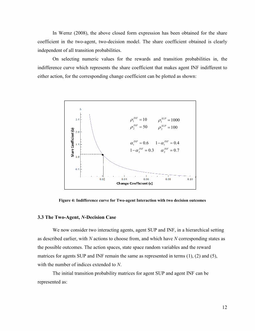
In Wernz (2008), the above closed form expression has been

coefficient in the two-agent,

independent of all transition probabilities.

On selecting numeric values for the rewards and transition probabilities in, the

indifference curve which represents the share coefficient that makes agent INF indifferent to

either action, for the corresponding change coefficient can be plotted as shown:

Figure 4: Indifference curve for Two

3.3 The Two-Agent, N-Decision Case

We now consider two interacting agents, agent SUP and INF,

as described earlier, with N actions to choose from, and

the possible outcomes. The action spaces, state space random variables

matrices for agents SUP and INF remain the same as represented in

with the number of indices extended to

The initial transition probability matrices for agent SUP and agent INF can be

represented as:

, the above closed form expression has been obtained for the share

, two-decision model. The share coefficient obtained is



curve which represents the share coefficient that makes agent INF indifferent to


Indifference curve for Two-agent Interaction with two decision outcomes

Decision Case

We now consider two interacting agents, agent SUP and INF, in a hierarchical setting

actions to choose from, and which have N corresponding

The action spaces, state space random variables and the reward

matrices for agents SUP and INF remain the same as represented in terms (1)

with the number of indices extended to N.

probability matrices for agent SUP and agent INF can be

1

2

10

50

INF

INF

ρ

ρ

=

=1

2

1000

100

SUP

SUP

ρ

ρ

=

=

1 1

2 2

0.6 1 0.4

1 0.3 0.7

INF INF

INF INF

α α

α α

= − =

− = =

12

obtained for the share

model. The share coefficient obtained is clearly


curve which represents the share coefficient that makes agent INF indifferent to


outcomes

in a hierarchical setting

corresponding states as

and the reward

), (2) and (5),

probability matrices for agent SUP and agent INF can be

13

11 1

1

SUP SUP

N

SUP

SUP SUP

N NN

P

α α

α α

=

…

⋮ ⋱ ⋮

⋯

,

11 1

1

INF INF

N

INF

INF INF

N NN

P

α α

α α

=

…

⋮ ⋱ ⋮

⋯

(16)

In order to ensure that the final transition probabilities in (10) sum up to one, the

general additive influence function is represented as follows:

( ),

| ,,1

SUP INF SUP

i j m

c i j

f s s a ci j

n

=

= −≠ −

, , , 1, 2,...i j m N= (17)

with 0c > , where n represents the number of outcomes associated with the two decisions that

the lower agent transitions between. When 2n = , the influence function represented in (8) is

obtained. The final transition probabilities are similar to the expressions presented in (10) and

(11), with the indices extending to N. Here, we make the simplifying assumption that change

coefficients for all outcomes are equal.

In order to describe a meaningful problem, the following assumptions can be made

without loss of generality:

• The agents have conflicting objectives; hence we can assume that the rewards have the

property that 1 2 ....SUP SUP SUP

nρ ρ ρ> > while1 2 ....INF INF INF

nρ ρ ρ< < .

• Agent SUP being in state 1

SUPs is favorable to the organization.

• To define a link between an action and the particular state that the agent intends to reach when

taking the action, we can assume that 1,SUP

mi m in

α > ∀ = and 1,INF

nj n jn

α > ∀ = , for all

, , , 1, 2,....i j m n n=

• { }0 min , , 1, 2,....SUP

mic m i nα≤ ≤ ∀ = is the assumption made to ensure the transition

probabilities do not exceed one.

We derive the expression for the share coefficient that causes a shift in agent INF’s

preferred strategy from action INF

na to an initially less favorable action INF

ma with agent SUP

taking action1

SUPa :

1 1| , | ,INF SUP INF INF SUP INF

final m final nE r a a E r a a ≥ , , 1, 2....m n N=

14

( ) ( ) ( )

( ) ( ) ( )

1

1 1

1

1 1

, | | ,

, | | ,

N NINF SUP INF INF INF INF SUP SUP INF SUP

final i j j m final i j

i j

N NINF SUP INF INF INF INF SUP SUP INF SUP

final i j j n final i j

i j

r s s p s a p s s a

r s s p s a p s s a

= =

= =

⇔ ⋅ ⋅ ≥

⋅ ⋅

∑∑

∑∑ (18)

By solving the expressions for the share coefficient for different values of N, we get:

( )

( )1

1

1

NINF INF INF

i mi ni

i

NSUP INF INF

i mi ni

i

nb

nc

ρ α α

ρ α α

=

=

− − ≥ −

−

∑

∑ (19)

( ) ( )

( )

1

1

1

1

nINF INF INF INF INF INF

n nn mn i mi ni

i

nSUP INF INF

i mi ni

i

nb

nc

ρ α α ρ α α

ρ α α

−

=

=

− − − − ≥ −

∑

∑ (20)

The above expression represents the optimal share coefficient for a two-agent interaction with

N decision alternatives and outcomes, when the agent shifts strategy from actionINF

na to actionINF

ma .

The share coefficient is dependent on the transition probabilities of agent INF, but independent of the

transition probabilities of agent SUP, thereby the same property observed in the two-agent two-

decision case is not observed here. In expression (20), the terms are rewritten such that they are

positive, as INF INF

nn mnα α> , with INF

nρ being the largest of all the rewards, due to the conflicting

objectives. The first term in the numerator must be large enough to make the share coefficient positive,

thereby making interaction feasible.

Since the expression can be used to move from the organization’s least preferred action n to

any action m , the cost of improving co-operation to the most preferred action, namely, when 1m = ,

can be evaluated, against the cost of moving to other intermediate actions. The organizational designer

can use this information to determine the level of co-operation that is affordable.

An important observation in (19) is that the transition probabilities that appear in the

expression are only those that describe agent INF’s transition to the outcomes associated with

the two decisions of interest – agent INF’s originally preferred strategy and the organization’s

preferred strategy. Hence, it is only the number of outcomes available to these decision

strategies that really affect the opt

alternatives.

Figure 5:

In Figure 4, the connectivity of the graph that represents the link between actions an

outcomes determines which transition probabilities appear in expression

conclude that even when N decision alternatives are present, only th

decision outcomes of the two decisions of interest determine the complexity of the optimal

share coefficient expression.

3.4 The Two-Decision Case

To understand why the two

probabilities, we substituten

2 1

2b

c

− ≥

Using the notation used in Wernz (2008

INFP

Substituting, we get:

b

strategies that really affect the optimal share coefficient, and not the actual number of decision

: Graph that represents actions and associated outcomes

In Figure 4, the connectivity of the graph that represents the link between actions an

outcomes determines which transition probabilities appear in expression (19)

decision alternatives are present, only the number of possible


Decision Case - A Special Case of the N-Decision Case

why the two-decision, two-outcome case is independent of all transition

2n = in expression (20):

( ) ( )( )( ) ( )

2 22 12 1 11 21

1 11 21 2 12 22

2 1

2

INF INF INF INF INF INF

SUP INF INF SUP INF INFc

ρ α α ρ α α

ρ α α ρ α α

− − −− − + −

Wernz (2008) for the two-agent two-decision model:

11 12 1 1

21 22 2 2

1

1

INF INF INF INF

INF

INF INF INF INFP

α α α αα α α α

−= =

−

( )( )( )( )

1 2 2 1

1 2 1 2

11

2 1

INF INF INF INF

INF INF SUP SUPb

c

α α ρ ρ

α α ρ ρ

− − − ≥ − − −

15

imal share coefficient, and not the actual number of decision

In Figure 4, the connectivity of the graph that represents the link between actions and

). Hence we

e number of possible


is independent of all transition

decision model:

16

( )( )2 1

1 22

INF INF

SUP SUPb

c

ρ ρ

ρ ρ

−≥

− (21)

The above expression is the same as expression (15). It can be seen that the two-

decision case with each decision having two possible is a special case of the N decision, N

outcome case, where the transition probabilities factor out of the expression, thereby making

the share coefficient independent of the probabilities. From the above result, we infer that

organizational designers benefit from restricting the number of decision outcomes to two, for

the two decisions of interest, whenever possible, due to the property of independence from

transition probabilities.

It is important to note that even when there are N decision alternatives, if the two

decisions of interest – agent INF’s originally preferred strategy and the organization’s

preferred strategy result in only two outcomes, then the optimal share coefficient is


Chapter 4

THREE-AGENT INTERACTION

4.1 The Three-Agent, Two-Decision Case

An MSDM model for three-agent interaction has been studied in Wernz and Henry

(2009), with each agent having two decision alternatives to choose from, resulted in two

associated outcomes. We extend the model to study the interaction among three agents with

each agent having N decision alternatives to choose from, with N associated outcomes. The

model presented in the above paper is explained below, to form the framework for our

extension.

The three interacting agents are represented as 1A , 2A and 3A , highest to lowest in

hierarchy, in the model. All three agents take a decision simultaneously, in a single decision

17

epoch. In the model presented in Wernz and Henry (2009), each agent has two decision

alternatives to choose from, their action spaces are represented as:

{ }1 2,Ax Ax AxA a a= , 1,2,3x = (22)

The state space random variable has the following realizations:

{ }1 2,Ax Ax AxS s s= , 1,2,3x = (23)

On taking a decision, ( )|p s a is the initial transition probability with which an agent

moves to the state corresponding to the action, without considering the influence from other

agents.

( )1 1 1|Ax Ax Ax Axp s a α= , ( )2 1 1

| 1Ax Ax Ax Axp s a α= −

( )1 2 2

| 1Ax Ax Ax Axp s a α= − , ( )2 2 2|Ax Ax Ax Axp s a α= (24)

We can assume that 1

2

Ax

iα > to link an action to its corresponding state (if an agent Ax takes

action Ax

ia , the most likely final state is Ax

is ).

Each agent receives a reward depending on the final state to which the agent moves on

receiving the reward.

( )Ax Ax Ax

i ir s ρ= , 1, 2; 1, 2,3i x∀ = ∀ = (25)

The reward matrices can be represented as:

1

2

Ax

Ax

AxR

ρρ

=

(26)

The model describes the interaction among agents through the influence that agents

have on each others’ rewards and transition probabilities. Each agent shares a portion of its

reward with its immediate subordinate (the agent exactly one level below). As a result, the

topmost agent indirectly shares a portion of its reward with the agent at the lowest level,

through the middle agent. The final state each agent moves to influences the transition

probabilities of its superior agents, and hence their expected reward when taking a particular

action. The interaction has been represented using a dependency graph in Wernz and Henry

(2009).

18

Mathematically, the portion of reward shared by an agent Axwith its immediate

subordinate, represented as , 1,2xb x = , is known as the share coefficient that agent Ax offers its

immediate subordinate. Since agent 1A shares a portion 1b of its reward with agent 1A , the

final reward it receives is:

( ) ( )( )1 1 1 1

11A A A A

final i ir s r s b= − (27)

Agent 1A receives a portion of agent 1A ’s reward, but it also shares a portion of its net

reward with agent 3A , its immediate subordinate. The final reward agent 2A receives can be

represented as:

( ) ( ) ( )( ) ( )2 1 2 2 2 1 1

1 1, 1A A A A A A A

final i j j ir s s r s b r s b= + ⋅ ⋅ − (28)

Agent 3A receives a share 2b of agent 2A ’s reward. Its final reward is mathematically

represented as:

( ) ( ) ( ) ( ) ( ) ( )3 1 2 3 3 3 2 1 2 3 3 2 2 1 1

2 2 1 2, , ,A A A A A A A A A A A A A A A

final i j k k final i j k j ir s s s r s b r s s r s b r s b b r s= + ⋅ = + ⋅ + ⋅ ⋅

With 1 20 , 1b b≤ ≤ (29)

To model the influence exerted by an agent on its superior’s transition probability,

influence functions xf , 1, 2x = for agents 1A and 2A are defined:

( ) 11 2

1

1

,,

,

A A

i j

c i jf s s

c i j

==

− ≠, ( ) 22 3

2

2

,,

,

A A

j k

c j kf s s

c j k

==

− ≠ (30)

xc , 1, 2x = is known as the change coefficient with which agent Ax influences its superior

agents’ transition probabilities, and describes the extent of influence the subordinate agents

have on its superiors.

Since 3A is the bottom most agent, its transition probabilities are not influenced by

any agent. However, agent 2A ’s transition probability is influenced by agent 3A ’s final state,

and is characterized through the influence function 2f :

( ) ( ) ( )2 2 2 3 2 2 2 2 3

2| , | ,A A A A A A A A A

final j n k j n j kp s a s p s a f s s= + (31)

The final transition probability of agent 1A , influenced by agent 2A directly and agent 3A

indirectly, is represented as:

19

( ) ( ) ( ) ( )( )1 1 1 2 3 1 1 1 1 2 2 3

1 2| , , | , 1 ,A A A A A A A A A A A A

final i n j k i n i j j kp s a s s p s a f s s f s s= + ⋅ + (32)

Since the transitions probabilities cannot exceed one,

{ }2 2 2 2

2 1 2 1 20 min , ,1 ,1A A A Ac α α α α< ≤ − − , ( ) { }1 1 1 1

1 2 1 2 1 20 1 min , ,1 ,1A A A Ac c α α α α< + ≤ − −

As in the two-agent interaction discussed in the previous section, we assume that the

topmost agent 1A always takes a decision to favor the organization, to reach state 1

1

As , which

is the state the organization most prefers. We assume that without considering the incentives

that are given by the superior agents, both agents 2A and 3A prefer states 2

2

As and 3

2

As

respectively; and hence prefer corresponding actions 2

2

Aa and 3

2

Aa which are most likely to

result in the outcome. In other words, the rewards have the properties that: 1 1

1 2

A Aρ ρ> while

2 2

1 2

A Aρ ρ<,

3 3

1 2

A Aρ ρ<

Once the share coefficients and change coefficients have been established, the decision

process begins, with each self interested expected utility maximizing agent choosing that

decision alternative which maximizes its expected reward. In order to switch the Nash

equilibria of agents 2A and 3A to a decision choice that favors the organization, the share

coefficients need to be sufficiently high.

To find the optimal share coefficient that agent 1A offers 2A , we need to determine

the value of b1 that causes agent A2 to shift its best response strategy from 2

2

Aa to 2

1

Aa , which

occurs when the expected rewards for the latter strategy is greater than that of the former.

When the expected rewards for both strategies are equal, agents pick the strategy that favors

the organization.

To find the optimal 1b we solve:

2 1 2 3 2 1 2 3

1 1 1 2| , , | , ,A A A A A A A A

final o final oE r a a a E r a a a ≥

( ) ( ) ( ) ( )

( ) ( ) ( ) ( )

2 1 2 1 1 1 2 3 2 2 2 3 3 3 3

1 1

1 1 1

2 1 2 1 1 1 2 3 2 2 2 3 3 3 3

1 2

1 1 1

, | , , | , |

, | , , | , |

n n nA A A A A A A A A A A A A A A

final i j final i j k final j k k o

i j k


final i j final i j k final j k k o

i j k

r s s p s a s s p s a s p s a


= = =

= = =

⇔ ⋅ ⋅ ⋅ ≥

⋅ ⋅ ⋅

∑∑∑

∑∑∑

20

( )( )

2 2

2 1

1 1 1

1 1 22

A A

A Ab

c

ρ ρ

ρ ρ

−≥

− (33)

Two important inferences are made from this result: Firstly, the share coefficient 1b is

independent of all transition probabilities. Secondly, 1b is indifferent to the decision made by

agent 3A .

To find the optimal share coefficient that agent 2A offers 3A , we need to determine

the value of 2b that causes agent 3A to shift its best response strategy from 3

2

Aa to 3

1

Aa . Here,

agent 2A has already been offered the optimal 1b , and has shifted strategy to favors agent 1A .

To find the optimal 2b we solve:

3 1 2 3 3 1 2 3

1 1 1 1 1 2| , , | , ,A A A A A A A A

final finalE r a a a E r a a a ≥

( ) ( ) ( ) ( )

( ) ( ) ( ) ( )

3 1 2 3 1 1 1 2 3 2 2 2 3 3 3 3

1 1 1

1 1 1

3 1 2 3 1 1 1 2 3 2 2 2 3 3 3 3

1 1 2

1 1

, , | , , | , |

, , | , , | , |

n n nA A A A A A A A A A A A A A A A

final i j k final i j k final j k k

i j k

n nA A A A A A A A A A A A A A A A

final i j k final i j k final j k k

j k

r s s s p s a s s p s a s p s a


= = =

= =

⇔ ⋅ ⋅ ⋅ ≥⇔

⋅ ⋅ ⋅

∑∑∑

∑∑1

n

i=∑

( )

( )( )3 3

2 1

2 2 2 1 1

2 2 1 1 1 1 22 3

A A

A A A Ab

c b c

ρ ρ

ρ ρ ρ ρ

−≥

− + − (34)

The above result shows that the share coefficient b2 is independent of all transition

probabilities.

In the following section, we study the three-agent interaction with each agent having N

decision alternatives to choose from instead of two. We characterize the results, and some

critical differences from the two decision alternative case.

4.2 The Three-Agent, N-Decision Case

The three interacting agents in the order of their hierarchy from highest to lowest are

1A , 2A , 3A . Each agent can choose from N different actions, the action spaces, state space

random variable and the reward matrices are similar to those defined in (22), (23), and (26),

with the indexes extending to N.

21

The transition probability with which an agent Ax reaches a particular state on choosing an

action, without considering the influence of agents lower in hierarchy is given by:

( )|Ax Ax Ax Ax

j i ijp s a α= , , 1, 2,....i j N= (35)

The initial transition probability matrix of agent x is given by:

11 1

1

Ax Ax

n

Ax

Ax Ax

n nn

P

α α

α α

=

…

⋮ ⋱ ⋮

⋯

(36)

The interaction between agents is similar to the structure described in the three-agent

two-decision alternative system, with each agent sharing a portion of its state-dependent

reward with its immediate subordinate. Each agent’s final state affects the transition

probability of its superiors, thereby impacting the probability with which they reach their

desired state.

In order to ensure that the final transition probabilities sum up to one, we introduce the

general influence function as:

( )1

1 2

1 1

,

,,1

A A

i j

c i j

f s s ci j

n

=

= ≠ −

, ( )2

2 3

2 2

,

,,1

A A

j k

c j k

f s s cj k

n

=

= ≠ −

(37)

where n represents the number of outcomes of the decisions that the agents switch between.

The interaction is graphically represented in Figure 6.

The final rewards and final transition probabilities remain the same for the agents 1A ,

2A , 3A as described in the three-agent, two-decision case. As before, the agents have

conflicting objectives; hence we can assume that the rewards have the property that

1 1 1

1 2 ....A A A

nρ ρ ρ> > while 2 2 2

1 2 ....A A A

nρ ρ ρ< < and 3 3 3

1 2 ....A A A

nρ ρ ρ< < .

To find the share coefficient that agent 1A offers 2A , we need to determine the value

of 1b that causes agent 2A to shift its best response strategy from 2A

na to an initially less

preferred strategy 2A

ma .

To find the optimal b1 we solve:

2 1 2 3 2 1 2 3

1 1| , , | , ,A A A A A A A A

final m q final n qE r a a a E r a a a ≥

22

( ) ( ) ( ) ( )

( ) ( ) ( ) ( )

2 1 2 1 1 1 2 3 2 2 2 3 3 3 3

1

1 1 1

2 1 2 1 1 1 2 3 2 2 2 3 3 3 3

1

1 1 1

, | , , | , |

, | , , | , |


final i j final i j k final j m k k q

i j k


final i j final i j k final j n k k q

i j k



= = =

= = =

⇔ ⋅ ⋅ ⋅ ≥

⋅ ⋅ ⋅

∑∑∑

∑∑∑

, , 1, 2,....m n q N=

( ) ( )

( ) ( )( )

2 2 2 2

11

2 2 3 1 1

1 2

1 1

1

1 1

nA A A

mi ni i

i

n nA A A A A

mi ni mi j j

i j

n

b

c c n n n

α α ρ

α α α ρ ρ

=

= =

− −=

− − + − −

∑

∑ ∑

(38)

We can see that b1 is dependent on the transition probabilities of agent 2A and agent

3A . Hence, 1b also is sensitive to the decision that agent 3A makes.

Influence on reward

Influence on transition

probability

3A

ns

3A

is

3

1

As2

1

Aa

2A

ia

2A

na

2

1

Aa

2A

ia

2A

na 2A

ns

2A

is

2

1

As

Agent

A2

1A

ns

1A

is

1

1

As

Agent

A1

1

1

Aa

1A

ia

1A

na

Agent

A3

Figure 6: Graphical Representation of Three-agent Interaction

23

To find the share coefficient that agent 2A offers 3A , we need to determine the value

of 2b that causes agent 3A to shift its best response strategy from 3A

na to an initially less

preferred strategy 3A

ma .

3 1 2 3 3 1 2 3

1 1| , , | , ,A A A A A A A A

final q m final q nE r a a a E r a a a ≥

( ) ( ) ( ) ( )

( ) ( ) ( ) ( )

3 1 2 3 1 1 1 2 3 2 2 2 3 3 3 3

1

1 1 1

3 1 2 3 1 1 1 2 3 2 2 2 3 3 3 3

1

1 1

, , | , , | , |

, , | , , | , |

n n nA A A A A A A A A A A A A A A A

final i j k final i j k final j q k k m

i j k

n nA A A A A A A A A A A A A A A A

final i j k final i j k final j q k k n

i j k



= = =

= = =

⋅ ⋅ ⋅ ≥

⋅ ⋅ ⋅

∑∑∑

∑∑1

n

∑(39)

Obtaining a closed form expression b2 is cumbersome, as the number of terms contained in

the expression is reasonably large. From the Mathematica code used to solve (39) for large

values of n , we observed can see that the b2 is dependent on the transition probabilities of

agents 2A and 3A .

As before, in order to describe a meaningful problem, the following assumptions are made

without loss of generality:

• To define a link between an action and the particular state that the agent intends to reach when

taking the action, we can assume that 1Ax

ijn

α > when i j= for all , 1, 2,....i j N= , 1,2,3x =

• { }1 20 , min , , 1, 2,.... ; 1, 2,3Ax

ijc c i j N xα≤ ≤ ∀ = = , to ensure the transition probabilities do

not exceed one.

4.3 The Two-Decision Case - A Special Case of the N-Decision Case

To understand why the two decision alternative case is independent of all transition

probabilities, while the n decision alternative case is not, we substitute 2n = in the 1b

expression:

( ) ( )

( ) ( )( )

22 2 2 2

1 2

11

2 22 2 3 1 1

1 1 2 2 1

1 1

2 1

2 1 2 1 2

A A A

i i i

i

A A A A A

i i i j j

i j

b

c c

α α ρ

α α α ρ ρ

=

= =

− −=

− − + − −

∑

∑ ∑

(40)

24

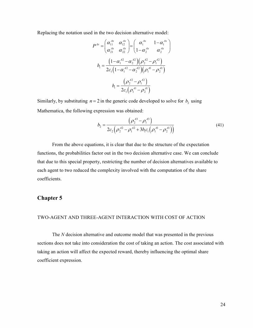
Replacing the notation used in the two decision alternative model:

11 12 1 1

21 22 2 2

1

1

Ax Ax Ax Ax

Ax

Ax Ax Ax AxP

α α α αα α α α

−= =

−

( ) ( )( )( )

2 2 2 2

1 2 2 1

1 2 2 1 1

1 1 2 1 2

1

2 1

A A A A

A A A Ab

c

α α ρ ρ

α α ρ ρ

− − −=

− − −

( )( )

2 2

2 1

1 1 1

1 1 22

A A

A Ab

c

ρ ρ

ρ ρ

−=

−

Similarly, by substituting 2n = in the generic code developed to solve for 2b using

Mathematica, the following expression was obtained:

( )( )( )

3 3

2 1

2 2 2 1 1

2 2 1 1 1 1 22 3

A A

A A A Ab

c b c

ρ ρ

ρ ρ ρ ρ

−=

− + − (41)

From the above equations, it is clear that due to the structure of the expectation

functions, the probabilities factor out in the two decision alternative case. We can conclude

that due to this special property, restricting the number of decision alternatives available to

each agent to two reduced the complexity involved with the computation of the share

coefficients.

Chapter 5

TWO-AGENT AND THREE-AGENT INTERACTION WITH COST OF ACTION

The N decision alternative and outcome model that was presented in the previous

sections does not take into consideration the cost of taking an action. The cost associated with

taking an action will affect the expected reward, thereby influencing the optimal share

coefficient expression.

25

5.1 Cost of Action in the Two-Agent Interaction Model

The expected rewards represented for agent INF contains a term INF

iδ , which

represents the cost of taking action i . The share coefficient is now calculated as:

( ) ( ) ( )

( ) ( ) ( )

1

1 1

1

1 1

, | | ,

, | | ,

N NINF SUP INF INF INF INF SUP SUP INF SUP INF

final i j j m final i j m

i j

N NINF SUP INF INF INF INF SUP SUP INF SUP INF

final i j j n final i j n

i j

r s s p s a p s s a

r s s p s a p s s a

δ

δ

= =

= =

⋅ ⋅ − ≥

⋅ ⋅ −

∑∑

∑∑

(42)

On solving, we get

( ) ( ) ( )

( )1

1

1 NINF INF INF INF INF

m n i mi ni

i

NSUP INF INF

i mi ni

i

n

ncb

δ δ ρ α α

ρ α α

=

=

−− − −

≥−

∑

∑ (43)

The above expression represents the optimal share coefficient when the cost of action

is considered. When compared to equation (19), the term ( )INF INF

m nδ δ− , the cost difference

between the two actions appears in the numerator. Hence if the scenario to be modeled

involves significant cost of action, the organizational designer should include the cost in the

evaluation of the optimal share coefficient.

5.2 Cost of Action in the Three-Agent Interaction Model

In the three-agent interaction model, when the cost of taking an action i for agent Ax ,

Ax

iδ is considered in the evaluation of the expected reward, the optimal share coefficients are

found to be:

( ) ( ) ( )

( ) ( )( )

22 2 2 2 2

11

2 2 3 1 1

1 2

1 1

1

1 1

nA A A A A

n m mi ni i

i

n nA A A A A

mi ni mi j j

i j

n

b

c c n n n

δ δ α α ρ

α α α ρ ρ

=

= =

− + − −=

− − + − −

∑

∑ ∑

(44)

In the above expression, the cost difference term appears in the numerator, similar to the two

agent case analyzed in (43). For 2b a similar behavior was observed, with the cost difference

26

term, for the two actions between which the switch takes place, featuring in the numerator for

large values of n . Again, obtaining a closed for expression for 2b for a general case is

cumbersome.

Chapter 6

DISCUSSION, CONCLUSION AND FUTURE RESEARCH

6.1 Discussion

We proceed to discuss some of the aspects of the Multiscale Decision-Making

(MSDM) model to enable an organizational designer to effectively implement the model. The

organizational designer must take care in measuring the organizational parameters, as the

input to the model will affect the accuracy of the results. Some aspects of the MSDM model

are discussed below.

6.1.1 On the Change Coefficient

The change coefficient defined in the MSDM model captures the influence that a

subordinate has on its superiors’ transition probabilities. The influence function considered in

this work is an additive influence function. The organizational designer needs to investigate

the nature of the interaction in the particular scenario being modeled, and may choose an

influence function that best fits the application. Alternate influence functions have been

discussed in (Wernz 2008). Since the model has been discussed in the function form, the

expectation expressions can be solved to compute the optimal share coefficient. To capture the

influence, the designer can use simulation techniques by studying historic data available on

decisions and outcomes. In the absence of robust data, eliciting information from experts is a

reasonable technique to use.

Scaling the data to ensure that the change coefficient is within its feasible limits is

critical. The change coefficient should be smaller than the smallest of transition probability

27

values, when additive influence functions are being considered, as shown in (9). In order to

define a meaningful model, the final transition probabilities should always sum to one. When

alternate influence functions are being considered, the range limits for the change coefficient

should ensure that the final transition probability does not exceed one. Accuracy in fixing the

change coefficient is critical to obtaining the optimal share coefficient that causes the Nash

equilibrium of the new game to align with the organizational goals.

6.1.2 On the Share Coefficient

The share coefficient represents the share of its reward that an agent is willing to share

with its subordinates, to obtain co-operation. When the optimal share coefficient is greater

than one, the reward structure that exists is insufficient to cause the lower-level agents to shift

strategy. Hence, the organizational designer receives insights about the rewards that the most

superior agent should be offered, so that the sharing of reward is feasible, thereby ensuring co-

operation.

When the share coefficient is negative, it indicates that for the given transition

probabilities, interaction is not feasible. On altering the transition probabilities, interaction is

feasible once again, for the same reward structure and agent hierarchy. This enables the

organizational designer to understand the organization better, and work towards altering

transition probabilities by changing the organizational environment, whenever possible.

6.2 Conclusion

The Multiscale Decision-Making (MSDM) model was extended to include N decision

alternatives and associated outcomes. The optimal share coefficient expressions were

developed for the general case, for two-agent interactions and partially for three-agent

interactions.

In the two-agent interaction model, the optimal share coefficient was found to be

dependent on the transition probabilities of the infimal agent, when the number of decision

alternatives and associated outcomes were increased above two. On further investigation, we

concluded that the number of possible decision outcomes for the two decisions of interest –

28

agent INF’s originally preferred strategy and the organization’s preferred strategy, affected the

transition probabilities that appeared in the optimal share coefficient expression. This suggests

to the organizational designer that the number of decision alternatives does not affect the

optimal share coefficient but it is only the number of decision outcomes that affects it. Hence,

there is benefit to restricting the number of decision outcomes available for the two decision

of interest to two, as the optimal share coefficient is independent of transition probabilities.

For the three-agent interaction model, expressions were developed for the optimal

share coefficients for agent 2A , but the expression for the optimal share coefficient for agent

3A was cumbersome. It was found that as the number of decision alternatives and associated

outcomes were increased beyond two, the optimal share coefficients at each level were

dependent on transition probabilities of all the agents superior in hierarchy. As the expression

was cumbersome, and useful properties were hard to elicit. Again, there is benefit to

restricting the decision outcomes available for the two decisions of interest at each level, as

the optimal share coefficients are independent of all transition probabilities. The cost of taking

a decision was incorporated into the MSDM model, and it was found that the optimal share

coefficient is affected by the difference in cost between the two decision alternatives of

interest.

It is clearly seen that as the number of agents increase, closed form expressions get

less tractable. When the number of hierarchies increases, organizational designers can resort

to generating the indifference curve of solving the expectation to identify the optimal share

coefficient graphically.

6.3 Future Research

The MSDM model integrates hierarchical and temporal scales of decision-making in

an organization. This work contributes to the hierarchical portion of MSDM, with general

models for the two-agent and three-agent hierarchical interactions being established. A

general model capturing temporal scale interactions would possibly lead to some interesting

observations, and help the organizational designer better understand how optimal share

coefficients behave when the parameters change with time.

29

Two-agent and three-agent interactions in the hierarchical scale have been studied.

Certain patterns seem to be emerging as the number of agents is increased. A vertical

generalization, for an N agent interaction would provide further understanding about the

behavior of the optimal share coefficient, and suggest to the designer if there is any benefit in

increasing or restricting the number of hierarchical levels. Modeling the influence function as

the number of agents grows beyond three is yet to be explored.

The influence function chosen to model interaction significantly impacts the optimal

share coefficient and the organizational parameters it depends on. The current model assumes

that all non-cooperative outcomes are equally bad. In the pursuit of taking the MSDM model

closer to real-world applications, considering influence functions where the change coefficient

c is not a constant may be useful to model a wider range of hierarchical interactions.

Exploring various influence functions and identifying the properties of the optimal share

coefficient would certainly expand the horizon of applications of MSDM.

References:

Chen, X., K. Yamauchi, et al. (2006). "Using the balanced scorecard to measure Chinese and

Japanese hospital performance." International Journal of Health Care Quality Assurance

19(4): 339-350.

Deng, X. and C. H. Papadimitriou (1999). "Decision-Making by Hierarchies of Discordant

Agents." Mathematical Programming 86: 417-431.

Fershtman, C. and K. L. Judd (1987). "Equilibrium incentives in oligopoly." The American

Economic Review: 927-940.

Grossman, S. J. and O. D. Hart (1983). "An analysis of the principal-agent problem."

Econometrica: Journal of the Econometric Society: 7-45.

Hallisy, J. A. and W. H. Haskel (2009). "The Empowered Patient Coalition."

Harris, M., C. H. Kriebel, et al. (1982). "Asymmetric Information, Incentives and Intrafirm

Resource Allocation." Management Science( 28): 604-620.

Harris, M. and A. Raviv (2002). "Organization Design." Management Science(48 ): 852-865.

Holmstrom, B. and P. Milgrom (1987). "Aggregation and linearity in the provision of

intertemporal incentives." Econometrica: Journal of the Econometric Society: 303-328.

30

Holmstrom, B. and P. Milgrom (1991). "Multitask principal-agent analyses: Incentive

contracts, asset ownership, and job design." JL Econ. & Org. 7: 24.

Jewitt, I. (1988). "Justifying the first-order approach to principal-agent problems."


Knott, A. M. (2001). "The dynamic value of hierarchy." Management Science 47(3): 430-448.

Lanier, D. C., M. Roland, et al. (2003). "Doctor performance and public accountability." The

Lancet 362(9393): 1404-1408.

Milgrom, P. R. and J. Roberts (1992). Economics, organization and management, Prentice-

Hall International.

Prat, A. (1997). "Hierarchies of processors with endogenous capacity." Journal of Economic

Theory 77(1): 214-222.

Qian, Y. (1994). "Incentives and loss of control in an optimal hierarchy." The Review of

Economic Studies 61(3): 527-544.

Rogerson, W. P. (1985). "The first-order approach to principal-agent problems."


Schneeweiss, C. (2003). Distributed Decision Making. Berlin, Springer

Vroom, G. (2006). "Organizational Design and the Intensity of Rivalry." Management

Science 52: 1689-1702.

Werner, R. M. and E. T. Bradlow (2006). "Relationship between Medicare’s hospital compare

performance measures and mortality rates." JAMA: the journal of the American Medical

Association 296(22): 2694-2702.

Wernz, C. and A. Deshmukh (2007). "Decision strategies and design of agent interactions in

hierarchical manufacturing systems." Journal of Manufacturing Systems 26(2): 135.

Wernz, C. and A. Henry (2009). "Multi-Level Coordination and Decision-Making in Service

Operations " Service Science 1(4): 270-283.

Wernz, C. L. (2008). Multiscale decision-making : bridging temporal and organizational

scales in hierarchical systems, University of Massachusetts Amherst: xii, 142 p.

Williamson, O. E. (1967). "Hierarchical Control and Optimum Firm Size." The Journal of

Political Economy 75: 123-138.

Documents

Multiscale Decision-Making for Multiple Decision … Singh for her detailed account of hospital organizational environments, which impacted my thesis significantly