Embed Size (px)
Citation preview

9/12/2002, Revised as recommended in review
Multiscale Medial Loci and Their Properties
Stephen M. Pizer Kaleem Siddiqi Gabor Székely James N. Damon Steven W. Zucker Computer Science Computer Science Electr. Engineering Mathematics Computer Science Univ of N.C. McGill University E.T.H. Univ. of N.C. Yale University
For submission to special UNC-MIDAG issue of IJCV
Abstract Blum's medial axes have great strengths, in principle, in intuitively describing object shape in terms of a quasi-hierarchy of figures. But it is well known that, derived from a boundary, they are damagingly sensitive to detail in that boundary. The development of notions of spatial scale has led to some definitions of multiscale medial axes different from the Blum medial axis that considerably overcame the weakness. Three major multiscale medial axes have been proposed: iteratively pruned trees of Voronoi edges [Ogniewicz 1993, Székely 1996, Näf 1996], shock loci of reaction-diffusion equations [Kimia et al. 1995, Siddiqi & Kimia 1996], and height ridges of medialness (cores) [Fritsch et al. 1994, Morse et al. 1993, Pizer et al. 1998]. These are different from the Blum medial axis, and each has different mathematical properties of generic branching and ending properties, singular transitions, and geometry of implied boundary, and they have different strengths and weaknesses for computing object descriptions from images or from object boundaries. These mathematical properties and computational abilities are laid out and compared and contrasted in this paper. 1. Introduction Methods for representing objects in 2D and 3D images can be divided into those that describe the boundary of the objects [Richards & Hoffman 1985] and those that describe the inside of the objects. The ones that describe the inside have certain advantages of multilocality. Of the ones that describe the inside, we can distinguish three categories: those that use globally prescribed components, e.g., geons; those based on generalized cylinders; and the medial methods. Because the geons [Biederman 1987] and the generalized cylinders [Marr & Nishihara 1978] require arbitrary decisions on how to choose the axis and the cross-sectional forms, many have preferred the medial representations. The medial methods extract an approximation to some subset of the symmetry set (also called herein the medial locus)1: {(x,r) | a disk (in 2D) or a sphere (in 3D) of radius r and centered at x is tangent to the object boundary at two separated positions or loci or at one position with order 2 tangency}. Equivalently, they can be thought to produce a locus of medial atoms, each made from two vectors of length r with a common tail x, where the vectors’ tips are incident to and normal to the boundary at the points of bitangency (Fig. 1). Blum’s axes [1967], defined before the symmetry set, are the subset of the symmetry set for which the bitangent disk or sphere is entirely contained within the object. The literature [Bruce et al. 1985] has already shown properties of the symmetry subset that are not held by the Blum subset. Blum’s skeleton has been widely influential in computer vision. It has roots in biology: Blum [1973] intuitively approximated a leaf by its veins, thus transforming a 2D region into a tree. And it has roots in the classical mathematics of the cut-locus in differential and Riemannian geometry. And it has implications for the visual 1 In Blum’s original work and much that followed, the symmetry set or the medial locus was taken to indicate simply the positional projection of the set under our definition, and the radius r was carried along as a separate function. In this paper when we use “medial locus” we mean a locus of (x,r) and when we use “symmetry set” we mean an x locus with an r value associated with each x.
1
9/12/2002, Revised as recommended in review
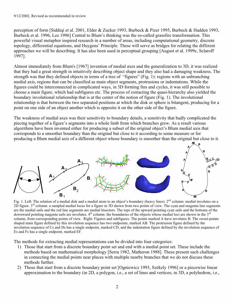
perception of form [Siddiqi et al. 2001, Elder & Zucker 1993, Burbeck & Pizer 1995, Burbeck & Hadden 1993, Burbeck et al. 1996, Lee 1996] Central to Blum’s thinking was the so-called grassfire transformation. This powerful visual metaphor inspired research in a number of areas, including computational geometry, discrete topology, differential equations, and Huygens’ Principle. These will serve as bridges for relating the different approaches we will be describing. It has also been used in perceptual grouping [August et al. 1999c, Sclaroff 1997]. Almost immediately from Blum's [1967] invention of medial axes and the generalization to 3D, it was realized that they had a great strength in intuitively describing object shape and they also had a damaging weakness. The strength was that they defined objects in terms of a tree of “figures” (Fig. 1): regions with an unbranching medial axis, regions that can be classified as main object segments, protrusions or indentations. While the figures could be interconnected in complicated ways, in 3D forming fins and cycles, it was still possible to choose a main figure, which had subfigures etc. The process of extracting the quasi-hierarchy also yielded the boundary involutional relationship that is at the center of the notion of figure (Fig. 1). The involutional relationship is that between the two separated positions at which the disk or sphere is bitangent, producing for a point on one side of an object another which is opposite it on the other side of the figure. The weakness of medial axes was their sensitivity to boundary details, a sensitivity that badly complicated the piecing together of a figure’s segments into a whole limb from which branches grew. As a result various algorithms have been invented either for producing a subset of the original object’s Blum medial axis that corresponds to a smoother boundary than the original but close to it according to some measure or for producing a Blum medial axis of a different object whose boundary is smoother than the original but close to it.
AA
BB
B•
••
•
••
A1
12
2
3
3
A
A
AD
B
B
B
B
DD
EE
F F
AB
CD
EF
BA
A
AB
CCC
Fig. 1. Left: The relation of a medial disk and a medial atom to an object’s boundary (heavy lines). 2nd column: medial involutes on a 2D figure. 3rd column: a sampled medial locus for a figure in 3D shown from two points of view. The cyan and magenta line segments are the medial sails and the red line segments are medial bisectors. The tops of the upward pointing cyan sails and the bottoms of the downward pointing magenta sails are involutes. 4th column: the boundaries of the objects whose medial loci are shown in the 3rd column, from corresponding points of view. Right: Figures and subfigures. The points marked A have involutes B. The sweet-potato shaped main figure defined by this involution sequence has two endpoints, marked AB. The protrusion figure defined by the involution sequence of Cs and Ds has a single endpoint, marked CD, and the indentation figure defined by the involution sequence of Es and Fs has a single endpoint, marked EF. The methods for extracting medial representations can be divided into four categories:
1) Those that start from a discrete boundary point set and end with a medial point set. These include the methods based on mathematical morphology [Serra 1982, Matheron 1988]. These present such challenges in connecting the medial points near places with multiple nearby branches that we do not discuss these methods further.
2) Those that start from a discrete boundary point set [Ogniewicz 1993, Székely 1996] or a piecewise linear approximation to the boundary (in 2D, a polygon, i.e., a set of lines and vertices; in 3D, a polyhedron, i.e.,
2

9/12/2002, Revised as recommended in review
a set of lines, tile edges, and vertices) [Lee 1982, Held 1998, Culver et al. 1999] and yield the continuous, connected set of Voronoi edges of the boundary set. The result is the special Blum subset of the symmetry set, in which the bitangent disks or spheres are fully contained in the object. This set of Voronoi edges must then be subject to an organization into limbs and branches by a sort of pruning process.
3) Those that start from a boundary curve or surface that is continuous in curvature, except perhaps at a few discrete points, and evolve via a partial differential equation representing a sort of grassfire that yields a distance function from the boundary [Kimia et al. 1990, Brockett & Maragos 1992, Haar 1994]. The medial locus, as well as points of relative maxima in width appear as singularities that result from shocks of the PDE solution that are labeled with the time of occurrence, i.e., the width of the figure, and with the type of shock. These shock types relate formally to the nature of the singularities that arise, for example whether it corresponds to an orientation discontinuity or to a boundary collision, and they can suggest categorical organizations of the shape. These methods also produce the Blum subset of the symmetry set, and they provide the possibility of determining the structure of limbs and branches as the PDE runs.
4) Those that start from the ambient space in which the object resides and look out toward a putative boundary, querying to what degree medial atoms at the points interact bilocally with the boundary, producing a scalar function on medial atoms called medialness. These methods are designed to operate on arbitrary greyscale images, avoiding the intermediate step of determining a boundary, but to allow comparison to the others, they will be assumed in this paper to be working on binary images representing the characteristic function of the object. The medial locus is provided as subdimensional maxima or saddles, called height ridges or height saddles, of medialness. The rules for choosing the dimensions for finding these critical loci will be discussed in section 3.3. This method is capable of producing not only an approximation to the Blum subset of the symmetry set but also other subsets, such as the vertical symmetry locus of a horizontally elongated object.
Methods of type 2 provide a solution to the problem of sensitivity to detail by the pruning process, where branches produced by detail are pruned away early. Methods of type 3 provide a solution to the sensitivity problem in two ways: by including a smallest scale via quantization of space and by including a notion of spatial scale on the distance transform, through which figures of small widths are not extracted. Methods of type 4 provide a solution by building width-proportional scale into measurement of the medialness function. By contrast, Blum described axes that today we describe as being at infinitesimal scale. The comparison of methods of types 2-4 are the subject of this paper. In particular, we describe an instance of type 2 and of type 3 and two versions of type 4:
2) Iteratively pruned trees of Voronoi edges of boundary points sets [Ogniewicz 1993, Székely 1996, Näf 1996].
3) Shock loci of Hamilton-Jacobi reaction-diffusion equations [Kimia et al. 1995, Siddiqi & Kimia 1996].
4) Height ridges and height saddles of medialness (cores) [Fritsch et al. 1994, Morse et al. 1993, Pizer et al. 1998]. Two forms of cores can be distinguished: a) the optimal parameter cores and b) the maximum convexity cores.
The main objective of this paper is to present the common properties and differences among symmetry sets, Blum medial loci, and the four categories of loci just listed. In particular, both qualitative differences in the generic structure of the loci and geometric differences will be mathematically presented. In addition, this paper will make some comparison in terms of strengths or weaknesses exhibited in computer implementations. Section 2 describes certain geometric properties of the symmetry set and the Blum medial axis, section 3 describes each of the methods in greater detail, section 4 compares mathematical properties of the medial loci
3
9/12/2002, Revised as recommended in review
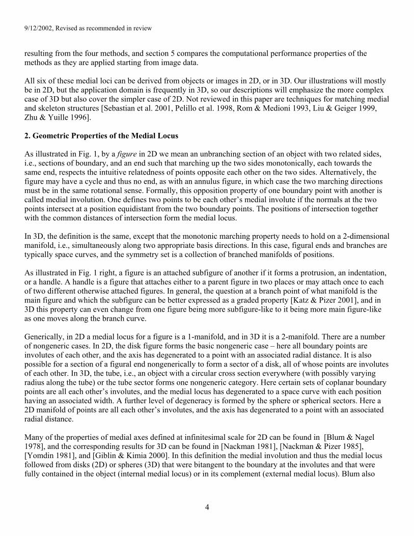
resulting from the four methods, and section 5 compares the computational performance properties of the methods as they are applied starting from image data. All six of these medial loci can be derived from objects or images in 2D, or in 3D. Our illustrations will mostly be in 2D, but the application domain is frequently in 3D, so our descriptions will emphasize the more complex case of 3D but also cover the simpler case of 2D. Not reviewed in this paper are techniques for matching medial and skeleton structures [Sebastian et al. 2001, Pelillo et al. 1998, Rom & Medioni 1993, Liu & Geiger 1999, Zhu & Yuille 1996]. 2. Geometric Properties of the Medial Locus As illustrated in Fig. 1, by a figure in 2D we mean an unbranching section of an object with two related sides, i.e., sections of boundary, and an end such that marching up the two sides monotonically, each towards the same end, respects the intuitive relatedness of points opposite each other on the two sides. Alternatively, the figure may have a cycle and thus no end, as with an annulus figure, in which case the two marching directions must be in the same rotational sense. Formally, this opposition property of one boundary point with another is called medial involution. One defines two points to be each other’s medial involute if the normals at the two points intersect at a position equidistant from the two boundary points. The positions of intersection together with the common distances of intersection form the medial locus. In 3D, the definition is the same, except that the monotonic marching property needs to hold on a 2-dimensional manifold, i.e., simultaneously along two appropriate basis directions. In this case, figural ends and branches are typically space curves, and the symmetry set is a collection of branched manifolds of positions. As illustrated in Fig. 1 right, a figure is an attached subfigure of another if it forms a protrusion, an indentation, or a handle. A handle is a figure that attaches either to a parent figure in two places or may attach once to each of two different otherwise attached figures. In general, the question at a branch point of what manifold is the main figure and which the subfigure can be better expressed as a graded property [Katz & Pizer 2001], and in 3D this property can even change from one figure being more subfigure-like to it being more main figure-like as one moves along the branch curve. Generically, in 2D a medial locus for a figure is a 1-manifold, and in 3D it is a 2-manifold. There are a number of nongeneric cases. In 2D, the disk figure forms the basic nongeneric case – here all boundary points are involutes of each other, and the axis has degenerated to a point with an associated radial distance. It is also possible for a section of a figural end nongenerically to form a sector of a disk, all of whose points are involutes of each other. In 3D, the tube, i.e., an object with a circular cross section everywhere (with possibly varying radius along the tube) or the tube sector forms one nongeneric category. Here certain sets of coplanar boundary points are all each other’s involutes, and the medial locus has degenerated to a space curve with each position having an associated width. A further level of degeneracy is formed by the sphere or spherical sectors. Here a 2D manifold of points are all each other’s involutes, and the axis has degenerated to a point with an associated radial distance. Many of the properties of medial axes defined at infinitesimal scale for 2D can be found in [Blum & Nagel 1978], and the corresponding results for 3D can be found in [Nackman 1981], [Nackman & Pizer 1985], [Yomdin 1981], and [Giblin & Kimia 2000]. In this definition the medial involution and thus the medial locus followed from disks (2D) or spheres (3D) that were bitangent to the boundary at the involutes and that were fully contained in the object (internal medial locus) or in its complement (external medial locus). Blum also
4
9/12/2002, Revised as recommended in review
defined the “generalized” medial locus by dropping the containment requirement, and this led to the notion of symmetry sets, studied mathematically by Bruce & Giblin [1986] and Giblin & Kimia [1999]. Blum & Nagel showed that in 2D the medial axis was generically a locus of branching curves with associated radial distances: x(s), r(s). Yomdin [1981], Nackman [1981], and Mather [1983] studied the medial locus and showed that it was generically a locus of branching sheets with associated radial distances: x(s), r(s), where s is a 2-vector of parameters. For 2D and 3D Yomdin and Mather determined the stability and generic local forms for the branching, relating them to specific singular properties of the function measuring distance from a point in space to the object boundary. For 3D Nackman determined the geometry of the boundary at nonbranching points of the medial locus points. Leyton [1987] showed that at end points of 2D Blum medial axes of figures, the doubly tangent disk becomes an osculating disk at boundary point that is a relative maximum of curvature. Bruce, Giblin, & Tari [1996] showed that for the 3D case, the sphere osculates the boundary surface at a crest point [Koenderink 1990] along the line of curvature with the smaller radius of curvature. Recently Giblin & Kimia [2000, 2002] have been classifying medial shock loci in 3D. A point on the medial locus (a position with its associated radial distance) implies a bitangent disk but does not communicate the corresponding points of boundary bitangency. To obtain this geometric information, we need the locus x(s), r(s), or more particularly, the first derivatives of x and r with respect to arc- or surface-distance along the positional medial locus x(s). In 2D the unit tangent vector b
r to the medial curve x(s) is equal to dx/ds,
where s is arclength along the positional medial axis. If we take derivatives in the direction of narrowing, dr/ds = cos(θ) gives the narrowing rate of the figure. Similarly, in 3D the derivatives of r with respect to distance on the medial surface give both the direction of maximal widening and its magnitude: if b
r is the unit vector on
the positional medial locus in the direction of maximal widening of the figure, then ∇ r = -cos(θ) br
. Moreover,
21 sx
sxnx ∂
∂×
∂∂
=r
xnr
normalized to unit length gives the direction normal to the positional medial locus. The cross-
product of with b is the unit vector in the tangent plane to x
r ⊥br
(s) that is in the level direction of r.
Combining these three vectors forms a medially fitted frame ( ))v,(),.(,( ubvubunx⊥),v that directionally
characterizes the figure locally.
rrr
Combining all this 0th and 1st order geometric information produces a “medial atom” with a medial point and two boundary-pointing vectors pr and
of common length r (Fig. 2). The common tail point of the vectors
gives the figural center xsr
, i.e., the medial position. The endpoints of these vectors are incident and normal to the two boundary position involutes py and sy ; that is, py = x + ( )bRr
xnb
rrr θ, ; sy = x + ( )bRr
xnb
rrr θ−, , where
( )θxnbR rr
, denotes an operator rotating its operand by the argument angle in the plane spanned by b xnrr, . The
bisector b of the two arrows together, in 3D, with the vector r
xnr normal to the medial surface span the space
containing pr and . b and bsrr ⊥r
span the tangent plane to x. The so-called “object angle” θ , between the bisector and the vectors yields the figural widening rate, cos(θ), which is equal to |∇ r|. Rotating b
r by θ± in
the plane yields the unit normals, and xnb rr, pr sr , to py and sy , respectively, so ( )bRr
xnbprr
rr θ,= and
( )bRrs nb x
rrrr= , θ− .
5
9/12/2002, Revised as recommended in review
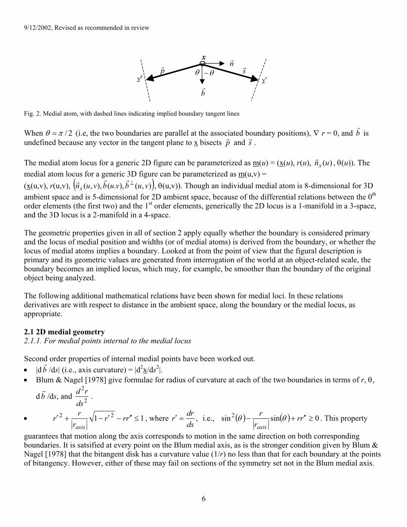
ysyppr θ θ−
x
sr
br
nr
Fig. 2. Medial atom, with dashed lines indicating implied boundary tangent lines When 2/πθ = (i.e, the two boundaries are parallel at the associated boundary positions), ∇ r = 0, and b
r is
undefined because any vector in the tangent plane to x bisects pr and sr . The medial atom locus for a generic 2D figure can be parameterized as m(u) = (x(u), r(u), )(unx
r , θ(u)). The medial atom locus for a generic 3D figure can be parameterized as m(u,v) = (x(u,v), r(u,v), ( )),(),.(),,( vubvubvunx
⊥rrr , θ(u,v)). Though an individual medial atom is 8-dimensional for 3D ambient space and is 5-dimensional for 2D ambient space, because of the differential relations between the 0th order elements (the first two) and the 1st order elements, generically the 2D locus is a 1-manifold in a 3-space, and the 3D locus is a 2-manifold in a 4-space. The geometric properties given in all of section 2 apply equally whether the boundary is considered primary and the locus of medial position and widths (or of medial atoms) is derived from the boundary, or whether the locus of medial atoms implies a boundary. Looked at from the point of view that the figural description is primary and its geometric values are generated from interrogation of the world at an object-related scale, the boundary becomes an implied locus, which may, for example, be smoother than the boundary of the original object being analyzed. The following additional mathematical relations have been shown for medial loci. In these relations derivatives are with respect to distance in the ambient space, along the boundary or the medial locus, as appropriate. 2.1 2D medial geometry 2.1.1. For medial points internal to the medial locus Second order properties of internal medial points have been worked out. r• |db /ds| (i.e., axis curvature) = |d2x/ds2|. • Blum & Nagel [1978] give formulae for radius of curvature at each of the two boundaries in terms of r, θ,
d /ds, and br
2
2
dsrd .
• 11 22 ≤′′−′−+′ rrrr
r
axisr , where ,
dsdrr =′ i.e., ( ) ( ) 0sin2 ≥′′+− rr
rr
axisθθsin . This property
guarantees that motion along the axis corresponds to motion in the same direction on both corresponding boundaries. It is satsified at every point on the Blum medial axis, as is the stronger condition given by Blum & Nagel [1978] that the bitangent disk has a curvature value (1/r) no less than that for each boundary at the points of bitangency. However, either of these may fail on sections of the symmetry set not in the Blum medial axis.
6

9/12/2002, Revised as recommended in review
2.1.2. For medial points bounding the medial locus (medial endpoints) Medial locus endpoints satisfy some additional relations, requiring derivatives that are one-sided limits.
• yp = ys = x + r b , i.e., the boundary point is of multiplicity 2 and θ=0. r
• dy/dsy • b = 0, where sy is arclength along either implied boundary section. r
• dr/ds = -1.
• The boundary curvature |d2y-/dsy2| = 1/r.
• The boundary curvature has a relative maximum, i.e., y is a vertex. 2.1.3. For nonregular medial points • The symmetry set can branch, cross, or have cusps [Bruce et al. 1985]. Crossing and cusp points do not
occur for the Blum medal axis. Crossing points and cusp points arise in the formation of a swallowtail section associated with encountering a protrusion or indentation in the boundary. 2.2. 3D medial geometry 2.2.1. Nongeneric objects The aforementioned tubular structures have 1-manifolds as medial loci and exhibit local rotational symmetry about the tangent vectors to these loci. That is, the xnr vector for a tubular medial atom is undefined and
becomes the set of all unit vectors orthogonal to br
, and similarly the y-x boundary-pointing vectors become the set of vectors based at x and of length r that have an angle θ with b
r. If we know that the figures of interest are
tubular, we would make an a priori decision to represent them by skeletal curves of medial atoms. In 2D there is the nongeneric case of the disk where the medial manifold is a point and the y-x boundary-pointing vectors become the set of all vectors of length r with a tail at x. The same case appears in 3D as the sphere. Other nongeneric cases are objects with sections of uniform r. In most natural objects in which the nongeneric symmetry appears, manifold sections of the generic type, i.e., slabs, appear in the same object. In this case it would be natural to represent the object in a mixed way by locally adapting the dimensionality of the skeleton to the type of the symmetry of the actual object subpart. The type of dominant symmetry can be locally well detected based on the differential geometric characterization of the height ridges of the distance map from the object boundary. Loci on distance ridges can be described by the eigenvectors and eigenvalues of the Hessian matrix of a slightly smoothed version of the Euclidean distance map from the boundary. In 3D, the negative Hessian matrix has three eigenvectors ( e 321 ,, ee rrr ) with the associated eigenvalues ( 321 ,, λλλ ). Three types of ridges can be identified: • 0-D ridges, where 0, 321 >>≈≈ λλλ . This indicates spherical symmetry. • 1-D ridges, where 0, 321 ≈>>≈ λλλ . This indicates tubular symmetry about a curvilinear axis. • 2-D ridges, where 0, 321 ≈≈>> λλλ . This indicates slabs having mirror symmetry about skeletal sheets.
7
9/12/2002, Revised as recommended in review
The statements in the following give additional general properties for the generic case where the medial locus is formed from branching 2-manifolds, i.e., where the object is made from slabs, not tubes. Versions of the property for tubes appear in parentheses. Define ynr to be the normal to the boundary y. 2.2.2. For medial points internal to the medial locus Nackman [1981] and Nackman & Pizer [1985] have given formulas for the mean curvature Hy and Gaussian curvature Ky of the medially implied boundary surfaces y as a function of the second fundamental form IIx for the medial surface, the Hessian of r (with derivatives in a medial tangent plane frame), and the first directional derivatives of r in the eigendirections of the Hessian in that frame. Analogous to the 2D case, at the points of bitangency the bitangent sphere’s curvature, 1/r, must be no less than the larger principal curvature2 at each
boundary, yyy KHH −+ 2 . Substituting Nackman’s formulas for Hy and Ky gives a constraint among r and
its derivatives with respect to distance along the medial locus x and the second fundamental form of x. As in 2D, there exists a locally weaker condition in 3D related to direction of motion on the boundary corresponding to that on the associated medial surface. For all Blum locus points this directional condition requires that 1/r is no less than the larger principal curvature of the surface parallel to the boundary at locally constant distance r into the figure from the boundary. 2.2.3. For medial points bounding the medial locus In the generic 3D situation, medial endpoints form an endcurve. (In the tubular case, medial endpoints are discrete points.) The general properties at this endcurve and special properties there listed in the following require that derivatives be on one half-plane (half-curve). r• y = x + r b , i.e., the boundary point is of multiplicity 2, and θ=0 (also applies for tubes).
r r• dyp/dsy • = dyb s/dsy • b = 0 (also applies for tubes). • κ1 = 1/r at both yp and ys ( for tubes, at all y in the set pointed to from x). • κ1 with 21 κκ > (and 21 κκ = for tubes) is a relative maximum of 1st principal curvature along the 1st
principal curve with positive curvature, i.e., y is a crest point. That is, at that crest point the boundary surface is osculated by the disk with radius 1 1/κ in the 1st principal direction with its center 1/1 κ− along the normal at y. That is, the end curve (point) of the medial axis is a cusp of the focal surface of the boundary. r
• is normal to the crest. b 2.2.4. For nonregular medial points • Medial locus branch point positions are generically formed when precisely three medial surfaces meet (at
the same (x,r)). These branch points generically form themselves into curves. The branch curves can end, corresponding to the formation of a fin, and the symmetry set, but not the Blum medial axis, can also have cusps, crossings, and swallowtails.
2 Contrary to the normal mathematics sign convention, we take convex objects to have positive curvature.
8

9/12/2002, Revised as recommended in review
2.3 Medial loci based on object-included disks or spheres The Voronoi and Hamilton-Jacobi equation shock loci described in this paper yield approximations to the Blum medial loci, in which the disks bitangent to the boundary are wholly contained within the object. Seeing the medial position of this disk center at a position equidistant from the boundary points along their normals suggests viewing the properties of the distance map from the boundary. Creation of the distance map is analogous to lighting a grass fire at the boundary and watching it progress. The medial locus can be characterized as the ridge in this distance map, a ridge at which the distance function is not C1 continuous. 2.3.1. Branch Significance The grassfire analogy is useful because, as proposed early by Blum, it leads to a measurement of branch importance, allowing the formation of limbs and branches that result in the graph description of the object in terms of figures and subfigural protrusions. It defines skeleton branch importance by using the velocity of skeleton branch formation to measure the “smoothness” of fronts as they collapse at symmetry points. Fig. 3 illustrates this concept. The original object boundary, shown as a bold line, generates a continuous fire-front. The front positions after some discrete time intervals are shown as dotted lines. The skeleton is developing with speed indicated by the vector v . It can be easily shown that ||r ||vr , the speed of skeleton formation, is proportional to1 )2/sin(/ θ , where 2θ is the angle at which the fire-fronts meet. As the opposite boundary segments become more and more parallel, θ will converge to 0, leading to infinitely fast skeleton formation. Blum suggested regarding a skeletal branch as more important as its corresponding boundary segments are more parallel and thus as the speed of its formation increases.
Fig. 3: Speed of skeleton formation by fire front quenching. The original object outline is denoted by bold lines, different discrete stages of the fire-front development are shown dotted. ydsydt /=
r is the tangent to the fire-front, 2θ is the angle of the meeting
fronts. The skeleton formation speed || ||vr will therefore be proportional to 1 )2/sin(/ θ .
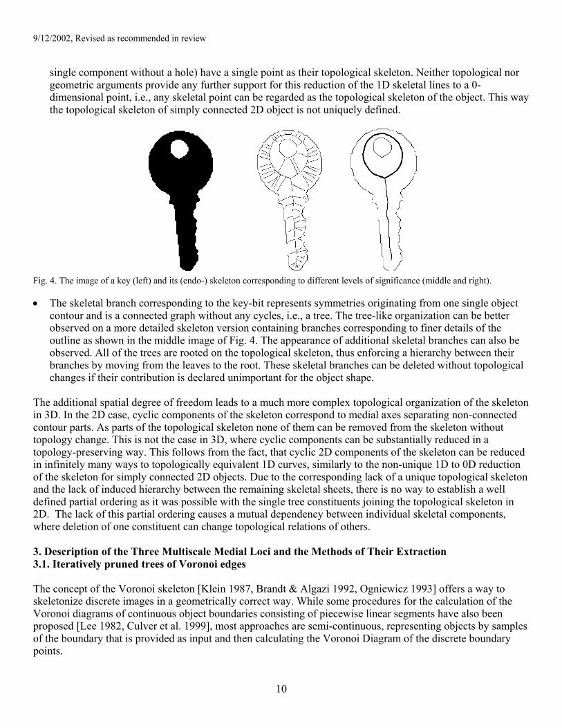
2.3.2 Medial Axis Topology The skeleton is a planar graph in 2D, making its topological structure very simple as illustrated by Fig. 4. Closer investigation of the skeleton presented on the right reveals that this actually consists of two different parts: • One part of the skeleton represents basically the symmetry between the contour of the hole in the key and its
external outline. This part of the skeleton is shown in bold on the figure. This skeletal part is a cycle and no part of it can be deleted without changing the skeletal topology. This corresponds to the fact that the boundary of the key can only be represented by two unconnected contours. We shall use the term topological skeleton to refer to the part of the skeleton which cannot be further contracted without topological changes (in the homotopy type). Objects with the topology of a disk (i.e., consisting of one
9
9/12/2002, Revised as recommended in review
single component without a hole) have a single point as their topological skeleton. Neither topological nor geometric arguments provide any further support for this reduction of the 1D skeletal lines to a 0-dimensional point, i.e., any skeletal point can be regarded as the topological skeleton of the object. This way the topological skeleton of simply connected 2D object is not uniquely defined.
Fig. 4. The image of a key (left) and its (endo-) skeleton corresponding to different levels of significance (middle and right).
• The skeletal branch corresponding to the key-bit represents symmetries originating from one single object
contour and is a connected graph without any cycles, i.e., a tree. The tree-like organization can be better observed on a more detailed skeleton version containing branches corresponding to finer details of the outline as shown in the middle image of Fig. 4. The appearance of additional skeletal branches can also be observed. All of the trees are rooted on the topological skeleton, thus enforcing a hierarchy between their branches by moving from the leaves to the root. These skeletal branches can be deleted without topological changes if their contribution is declared unimportant for the object shape.
The additional spatial degree of freedom leads to a much more complex topological organization of the skeleton in 3D. In the 2D case, cyclic components of the skeleton correspond to medial axes separating non-connected contour parts. As parts of the topological skeleton none of them can be removed from the skeleton without topology change. This is not the case in 3D, where cyclic components can be substantially reduced in a topology-preserving way. This follows from the fact, that cyclic 2D components of the skeleton can be reduced in infinitely many ways to topologically equivalent 1D curves, similarly to the non-unique 1D to 0D reduction of the skeleton for simply connected 2D objects. Due to the corresponding lack of a unique topological skeleton and the lack of induced hierarchy between the remaining skeletal sheets, there is no way to establish a well defined partial ordering as it was possible with the single tree constituents joining the topological skeleton in 2D. The lack of this partial ordering causes a mutual dependency between individual skeletal components, where deletion of one constituent can change topological relations of others. 3. Description of the Three Multiscale Medial Loci and the Methods of Their Extraction 3.1. Iteratively pruned trees of Voronoi edges The concept of the Voronoi skeleton [Klein 1987, Brandt & Algazi 1992, Ogniewicz 1993] offers a way to skeletonize discrete images in a geometrically correct way. While some procedures for the calculation of the Voronoi diagrams of continuous object boundaries consisting of piecewise linear segments have also been proposed [Lee 1982, Culver et al. 1999], most approaches are semi-continuous, representing objects by samples of the boundary that is provided as input and then calculating the Voronoi Diagram of the discrete boundary points.
10
9/12/2002, Revised as recommended in review
The Voronoi skeleton concept can easily be understood by the grassfire analogy, with the discrete boundary points set on fire. If the fire is evolving isotropically, circular fire-fronts are generated by each of these local fires which will then quench at exactly the Voronoi edges. This analogy suggests intuitively that the Voronoi diagram of the discrete boundary point set should strongly resemble the skeleton of the object. Methods of mathematical morphology can be used to prove that if the density of the boundary sampling goes uniformly to infinity, the Voronoi diagram of the point set (excluding Voronoi edges separating neighboring sampling points) will converge to the skeleton of the object [Schmitt 1989]. While the Voronoi Diagram of the boundary sample points contains branches approximating the skeleton of the object, conceptually it is very different from the skeleton of an object. Only a part of the available information, the geometric position of the sample points, has been used for its generation. In order to handle the topological issues of the skeleton generation, a topology has to be enforced on this discrete point set. Proximity relations on the original object boundary can be used to define a neighborhood topology between these points. Informally speaking, the connecting lines between boundary neighbors define a continuous polygonal approximation of the original object and will cut the Voronoi Diagram into an internal and external part corresponding to the internal (endo-) and external (exo-) skeleton by cutting the Voronoi edges separating neighboring points on the contour. The topology of this partial Voronoi diagram can then be investigated and a homotopy equivalence can be established between it and the original object. The Voronoi technique includes a phase of deciding at a branch point which is the limb and which the offshooting branch. This choice, based on the importance of individual skeletal branches described in section 2.3.1, forms the regularization of Voronoi skeleton, which is mandatory as a result of the discreteness of the boundary. Accordingly, no further attention has to be paid to regularization once a sound skeletal scale space has been defined. The general strategy is to let the offshoot be the branch of lesser significance. Two fundamentally different strategies have been developed to measure the significance of a skeletal branch (a detailed analysis of and examples for these measures are given in Section 4.2): • Figural significance measures express the significance of a skeletal branch by measuring the importance of
a figure/subfigure complex for the overall appearance of the object. It can be shown that due to the simple topological structure of the Delaunay triangulation it is possible to associate a subpart of the object with a single Delaunay edge. Duality can carry over this association to Voronoi edges, i.e. skeletal branches.
• Local significance measures estimate the importance of a skeletal point by calculations based on locally defined geometrical measurements on the Voronoi and/or Delaunay constituents.
Ideally one can work from the inside trunk to the outside twigs via the topological skeleton, and this is indeed the method applied in 2D, based on skeletal branch tracking using figural significance measures discussed in Section 4.2. In 3D it is necessary to work from the outside twigs back to the trunk. The lack of a topologically defined skeletal hierarchy makes the implementation of peeling strategies necessary, where topology preservation has to be explicitly checked.
11

9/12/2002, Revised as recommended in review
3.2. Shock loci of a reaction-diffusion equation
Fig. 5. The deformation of an initial curve is described by the displacement of each point in the tangential and normal directions. A second method for obtaining the internal medial axis of an object, given its bounding curve or surface, is to simulate the grassfire using a partial differential equation. An arbitrary deformation of a 2D closed curve is illustrated in Fig. 5, where each point on an initial curve is displaced by a velocity vector with components in the tangential and normal directions. Without loss of generality, it is possible to drop the tangential component (by a reparametrization of the evolved curve). Kimia et al. [1995] proposed the following evolution equation for 2D shape analysis: ).()0,(;)1( 0 pCpCNt =+= ακC
r Here ),( tpC is the vector of curve coordinates,
),( tpNr
is the inward normal, p is the curve parameter, t is the evolutionary time of deformation, and )(0 pC is the initial curve. The constant α ≥ 0 controls the regularizing effects of curvature κ . The case where α = 0 results in the grassfire flow. The equation is hyperbolic, and the locus of points at which shocks or entropy satisfying singularities form [Lax 1971], along with their times of formation, gives the positional medial axis and the associated radius function, respectively. The extension to 3D is obtained by replacing the closed curves with closed surfaces ),,( tqpS , where p,q is the surface parametrization. The numerical simulation of the grassfire flow as a partial differential equation can be based on the use of level set methods developed by [Osher and Sethian 1988] and [Sethian 1996]. The essential idea is to represent the curve C( p,t ) or the surface S(p,q, t) as the zero level set of a smooth and Lipschitz continuous function Ψ : Rn × [0,τ ) → R, given by {X ∈Rn : Ψ(X, t) = 0}. By differentiating this equation with respect to t and then with respect to the parameters of the curve (or surface in 3D), it can be shown that for the evolving curve or surface to satisfy the grassfire flow, the embedding surface Ψ must evolve according to Ψt =|| ∇Ψ || . The equation is solved by first discretizing the problem and then using numerical techniques derived from hyperbolic conservation laws. The main advantage of this formulation is that the embedding surface remains a graph (an Rn → R mapping), allowing topological changes to the evolving curve (or surface in 3D) to be handled automatically. The embedding surface may also be used to detect shocks by interpolation, as in [Siddiqi & Kimia 1996, Siddiqi et al. 1997]. However, the computational complexity of such interpolation schemes can be very high, and their extension to 3D is not immediate. For related material, see [Shah 1996, Tari et al. 1997, Leymarie & Levine 1992, Kimmel et al. 1995, Gomez & Faugeras 2000, Cross & Hancock 1997, Tari et al. 1997] We now consider an alternate formulation of the grassfire flow as a Hamilton-Jacobi equation on the Euclidean distance function to the initial curve [Siddiqi et al. 1999, 2002], which leads to an algorithm for computing skeletons in 2D and 3D with far better performance. In physics, such equations are typically solved by looking at the evolution in the phase space of the equivalent Hamiltonian system.
12
9/12/2002, Revised as recommended in review
More specifically, let be the Euclidean distance function to th boundar D e y C of the object. The magnitude of its gradient, || ∇D || , is identical to 1 in its smooth regime. For
r q = (x,y),
r p = (Dx , Dy ) with || 1||=pr , and the
associated Hamiltonian function H = 1− || ∇D ||, the Hamiltonian system is given by ),(
)0,0(
yx DDH=
−=
/
/
p
qH
−=
=rq
p&r
r&r
∂
∂
∂
∂.
This is a formulation of the grassfire flow with the following interpretation of the evolution of the phase space (r p ,
r q ) of the system: the gradient vector ∇ does not change with time and each point on the boundary of the
curve moves by an amount proportional to its components. We approach the discrimination of medial from non-
medial axis points by computing the “average outward flux” of the vector field about a point. The average outward flux is the outward flux through the boundary of a region containing the point, normalized by the
length of the boundary
D
.qr
)R
ds
∂
>
(
,
length
NqR∫ <
∂
r&r
. Here ds is an element of the bounding contour ∂R of the region R , and
is the outward normal at each point on the contour. By the divergence theorem r N
.
div(
r q .
R∫ )da = <
r q ,
r N > ds
∂R∫ , where da is an area element. Thus the outward flux is related to the divergence by
a
dsNq
aqdiv R
∆
∫ ><
→∆= ∂
r&r
&r,
0lim
)( , where ∆ is the area of the region a R . The integral of the divergence of
q&r within a region, or equivalently the outward flux through this region's bounding contour, measures the degree to which the flow generated by q&r is area preserving. Specifically, it, and thus the average outward flux, is negative in neighborhoods where the flow is area decreasing, positive where it is area increasing and zero otherwise. However, it can be shown that as the region shrinks to a point not on the medial axis, the average flux approaches zero. The usual divergence theorem does not apply for regions containing part of the medial axis. Instead, we consider the limiting behavior of the average outward flux as the region over which the integral is computed shrinks to a medial axis point. It can be shown that this quantity approaches a strictly negative number proportional to nq r&r, , where n is the normal to the medial axis and the constant of proportionality depends on
whether the axis point is a regular point or a branch point. Thus, the average outward flux calculation remains an effective way of detecting singularities of the vector field
r
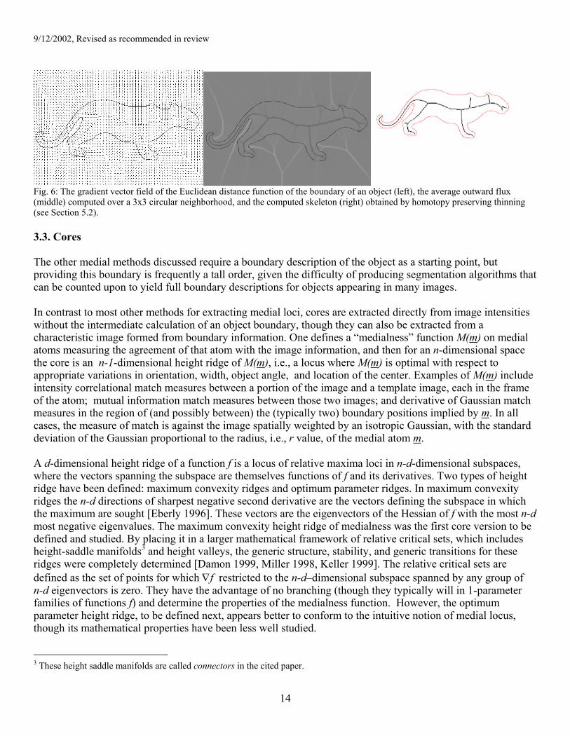
q&r : non-medial points give values that are close to zero and medial points corresponding to strong singularities give high negative values. Fig. 6 illustrates this average outward flux computation on a panther object, where values close to zero are shown in medium grey. All computations are carried out on a rectangular lattice, although the bounding curve is shown in interpolated form. Strong singularities correspond either to high magnitude negative (dark grey) or positive numbers (light grey), depending upon whether the vector field is collapsing at or emanating from a particular point (Fig. 6, left and middle). The extension of the above formulation to 3D is simply to replace the initial closed curve with a closed surface S , to add a third coordinate z to the phase space of the Hamiltonian system, and to replace the area element with a volume element and the contour integral with a surface integral when computing the average outward flux. This approach enjoys an intuitive relationship to the involute definition of a figure in section 2, with the normals now opposing at the skeleton rather than from the boundary.
13
9/12/2002, Revised as recommended in review
Fig. 6: The gradient vector field of the Euclidean distance function of the boundary of an object (left), the average outward flux (middle) computed over a 3x3 circular neighborhood, and the computed skeleton (right) obtained by homotopy preserving thinning (see Section 5.2). 3.3. Cores The other medial methods discussed require a boundary description of the object as a starting point, but providing this boundary is frequently a tall order, given the difficulty of producing segmentation algorithms that can be counted upon to yield full boundary descriptions for objects appearing in many images. In contrast to most other methods for extracting medial loci, cores are extracted directly from image intensities without the intermediate calculation of an object boundary, though they can also be extracted from a characteristic image formed from boundary information. One defines a “medialness” function M(m) on medial atoms measuring the agreement of that atom with the image information, and then for an n-dimensional space the core is an n-1-dimensional height ridge of M(m), i.e., a locus where M(m) is optimal with respect to appropriate variations in orientation, width, object angle, and location of the center. Examples of M(m) include intensity correlational match measures between a portion of the image and a template image, each in the frame of the atom; mutual information match measures between those two images; and derivative of Gaussian match measures in the region of (and possibly between) the (typically two) boundary positions implied by m. In all cases, the measure of match is against the image spatially weighted by an isotropic Gaussian, with the standard deviation of the Gaussian proportional to the radius, i.e., r value, of the medial atom m. A d-dimensional height ridge of a function f is a locus of relative maxima loci in n-d-dimensional subspaces, where the vectors spanning the subspace are themselves functions of f and its derivatives. Two types of height ridge have been defined: maximum convexity ridges and optimum parameter ridges. In maximum convexity ridges the n-d directions of sharpest negative second derivative are the vectors defining the subspace in which the maximum are sought [Eberly 1996]. These vectors are the eigenvectors of the Hessian of f with the most n-d most negative eigenvalues. The maximum convexity height ridge of medialness was the first core version to be defined and studied. By placing it in a larger mathematical framework of relative critical sets, which includes height-saddle manifolds3 and height valleys, the generic structure, stability, and generic transitions for these ridges were completely determined [Damon 1999, Miller 1998, Keller 1999]. The relative critical sets are defined as the set of points for which ∇f restricted to the n-d–dimensional subspace spanned by any group of n-d eigenvectors is zero. They have the advantage of no branching (though they typically will in 1-parameter families of functions f) and determine the properties of the medialness function. However, the optimum parameter height ridge, to be defined next, appears better to conform to the intuitive notion of medial locus, though its mathematical properties have been less well studied. 3 These height saddle manifolds are called connectors in the cited paper.
14
9/12/2002, Revised as recommended in review
Optimum parameter height ridges [Fritsch et al. 1994, Furst 1999] recognize that certain of the parameters of a variable such as the medial atom m are in Euclidean space and others, in the case of the core those giving orientations, angles, or radial width, are geometrically special by explicitly needing optimization. In the case of the core we do not want to optimize along the core, but we do want for each medial atom on the core an optimal orientation (i.e., frame), an optimal object angle, and an optimal width, and as well we want the medial atom optimally placed in the direction normal to the positional projection, x, of the locus. Thus m is written as (x,p), where x gives a position in the “ambient space” of the image and the “parameters” p are the remaining arguments. The optimal parameter ridge involves maximizing f over p and having the non-maximizing directions be only in the ambient space x. Moreover, the choice of maximizing directions in the ambient space may depend on the orientations chosen in the maximization over the parameters. For example, for the space of medial atoms m, one wishes first to find loci that are optimal with respect to the radial width, the medial frame, and the object angle, and one wishes to maximize spatially over the direction(s) normal to the positional medial locus and thus given by the optimal frame. For the purposes of this paper the term core will be called maximum convexity core or optimum parameter core depending on the type of height ridge of medialness that is used. Hence, for each type of height ridge for nx ℜ∈ there is a natural rule for choosing an n-d-dimensional subspace V of ℜn so that x belongs to the height ridge provided that ( ) 0| =∇ Vxf and that the Hessian of f restricted to V is negative definite. This generalizes to define a height k-saddlepoint x as points where again ( ) 0| =∇ but for which the Hessian of f is negative definite in an n-d-k-dimensional subspace of V but non-negative definite in the remaining k dimensions.
Vxf
The methods for computing cores proceed from a seed point by climbing to the height ridge of medialness by an optimization technique and then following the ridge by either zero level surface following techniques [Furst 2001] or predictor-corrector differential equation solvers [Fritsch et al. 1994]. 4. Comparative Mathematical Properties of the Three Medial Loci 4.1 Contrasts and comparison of the loci and their extraction methods The three methods we are discussing are all methods which start from a boundary or a greyscale image of an object and yield a medial locus of unknown topology. These can be distinguished from methods which start from a known topology and deform it into the input data [Pizer et al. 2001]. The three methods we are discussing differ mathematically in a number of ways. Many of the items in the following brief discussion are expanded upon in sections 4.2-4. 4.1.1. How discreteness appears
In the Voronoi technique the boundary is discretized, and then the discrete problem is solved. In contrast, the curve/surface evolution and cores techniques still are solving a continuous problem but are approximating a continuous locus in the ambient space by a C0 curve or surface made from discrete components (pixelwise or voxelwise). For the latter techniques the numerical resolution can be improved by increasing the rate at which the underlying object is sampled.
15
9/12/2002, Revised as recommended in review
4.1.2. The type of mathematical definition The Voronoi and curve/surface evolution techniques are based on the behavior of the distance transform. The Voronoi technique deals with this by computational geometry on the relation between points in space. The curve/surface evolution technique differentially sweeps out the distance function, using its gradient to propagate the boundary until shocks are formed. The shock formation is detected by integration of the flux corresponding to the gradient vector field. The cores technique also combines an integration with differentiations. The medialness measure is a spatial integral of the result of a differentiation at each end of the medial atom, and the ridge finding is a process of maximization, which is essentially differential. The Voronoi technique localizes the medial locus directly from the boundary point positions, producing a precise locus but with error propagated from the discretization. In the curve/surface evolution and cores techniques localization occurs via an interpolation basis and thus is produced with tolerance.
4.1.3. What specifies the special points terminating and connecting simplified segments
Simplified segments are the segments between special points on the medial locus such as ends, branches, and minima or valleys of width. The different methods have different special points and find them differently. In handling branches, cores techniques work from the trunk out, starting from a seed. The maximum convexity core technique finds locus crossings at critical points, and the optimum parameter core must be extended to handle branching because of the nonexistence of true branch points, as described in section 4.4. In contrast, the Voronoi and curve/surface evolution techniques do find true branches and work from the outside branches in. The Voronoi technique labels as non-medial segments all linear Voronoi segments that divide neighboring boundary points and all points at which two such segments join as medial endpoints. Branch loci not involving two medial segments bound the medial segments and form the branch nodes in the medial graph. The curve/surface evolution technique labels shocks from two boundary points as part of a simplified segment and shocks evolving from earlier shocks, such as pinch loci and partial-sphere centers, as terminating simplified segments. In the grassfire formulation the detection of branch points in 2D is based on predicting when two distinct shock trajectories are about to collide, exploiting the property that orientation along a skeletal branch varies continuously [Siddiqi & Kimia 1996]. However, this approach can be sensitive to the time step of the numerical evolution and can fail when multiple branches form nearby one another. The Hamilton-Jacobi formulation is better able to handle the detection of branch points and end points [Dimitrov et al. 2000, Bouix & Siddiqi 2000, Siddiqi et al. 2002].
Unlike the other techniques, the cores technique requires explicit tests for ending of the medial locus. While some core ends can be identified via the transition of the height ridges of medialness into height saddles, core endcurves (3D) and endpoints (2D) typically require computing a ridge of end strength (“endness”). The Voronoi technique, and to a lesser degree curve/surface evolution, suffer from oversegmentation of the medial locus. They produce branchings for the tiniest of boundary pimples or dimples, and the Voronoi technique oversegments in consequence of the discrete subdivision of the boundary. In contrast, the cores technique can avoid responding to small scale boundary features but can suffer from undersegmentation, possibly both missing branches and not identifying as a continuous medial locus one core that is connected to another by a long sequence of medialness height saddles.
4.1.4. The simplified segments’ loci
Whereas the curve/surface evolution and cores techniques produce curvilinear simplified segments, the Voronoi technique produces a piecewise linear representation of the simplified segments. The distance ridge produced by the Voronoi and curve/surface evolution techniques and the height ridge of medialness are not precisely the same loci, even on binary images, as a result of the regularizing effect of the cores technique’s
16

9/12/2002, Revised as recommended in review
r-proportional interrogation of space, as a result of the behavior of cores of frequently changing from height ridges to height saddles of medialness near figure/subfigure intersections, and as a result of cores approximating the symmetry set near branches where the other two loci approximate the Blum medial locus.
4.1.5. The topology of the medial locus The Voronoi technique guarantees equivalence with the topology of the Blum skeleton. For the 2D case the topological structure of the partial Voronoi diagrams (internal or external) enforces a processing order on the branches that leads to straightforward simplification strategies. In 3D, the equivalence remains, but the complexity of the medial topology prevents a generalization of the 2D processing order and leads therefore to difficulties in significance assignment. The combination of the equivalence with these significance assessment difficulties leads to a difficulty in breaking loops in the medial locus that occur as a result of small scale errors that form holes in the segmentation providing the input to the medial locus formation. The cores techniques produces an approximation to the symmetry set, so it can yield external medial loci and loci describing more distant symmetries whose medial disk or sphere is only partially contained in the object. The other two techniques must take special steps to identify such loci. However, the extra loci that cores find bring with them complications of too many candidates when trying to discern the inter-figural structure. This difficulty is of special concern because of optimum parameter cores’ need to identify branching topology nonlocally, with the consequent possibility of both missing branches and creating incorrect branches. Cores also sometimes break, and the solution of height saddle following is not guaranteed to correctly join separated pieces of the same medial locus. Cores can also fail to close around a hole as a result of numerical errors and the multiplicity of height ridges that can exist in a region. In the grassfire formulation of the curve/surface evolution equation, the detection and tracking of shocks can be sensitive to both the numerical time step used to evolve the boundary as well as the resolution of the underlying grid. Erroneous topologies may arise due to the incorrect grouping together of shocks from distinct branches, particularly when these branches are nearby and have similar orientations. The Hamilton-Jacobi formulation is more robust since it uses a discretized measure of average outward flux to guide a topology preserving thinning process on a grid. Thus, it can guarantee that the topology of the underlying 2D or 3D binary object is preserved. However, the localization of branch points or curves and end points or curves, is sensitive to the resolution of the underlying grid. The various medial analysis techniques differ in how they handle nongeneric pieces of skeleton (especially tubes in 3D) and in how they behave in certain degenerate situations of the discrete approximation to the boundary of the object being analyzed. The cores technique can fail if it is searching for a 2-manifold height ridge where the height ridge degenerates to a 1-manifold as a result of encountering a section of tube. Numerical error can bring one into the generic behavior of missing the height ridge curve when ones attempt to climb to it on the hill of medialness. However, the 1-ridge can be found if you have a priori information of where the transition from 2-ridge to 1-ridge will occur. The curve/surface evolution formulation cannot handle the tracking of shocks arising from near parallel boundaries, no matter how small a time step is used, since their velocities become infinite. Instead alternate interpolation strategies have to be used [Siddiqi et al. 1997], which may alter the topology of the medial locus. The Hamilton-Jacobi formulation, however, overcomes this limitation since the detection of shocks does not require the bounding curve to be explicitly evolved. Instead, the average outward flux measure is used to guide a thinning process, as detailed in Section 4.3. Intuitively, near parallel boundaries, and thus tubes in 3D, will result in medial axis points having very high negative average outward flux values.
17
9/12/2002, Revised as recommended in review
Voronoi techniques require attention to degenerate relations among segments, such as cocircularity of 4-tuples of boundary points in the Voronoi technique discussed in this paper. However, these difficulties can be catalogued and solved, as has been already done in the existing algorithm. This solution can require exact arithmetic to be employed. The real difficulty occurs in near-degenerate, rather than degenerate, situations in 3D. With near-degeneracy the computed 2D medial locus branches bushily, and the inadequate behavior of the heuristic significance assessment methods available in 3D often prevent satisfactory resolution of the bushiness into main axis components and trivial branches.
4.1.6. The aspect and role of scale in medial locus formation While all medial techniques are necessarily bilocal across the figure, the techniques differ strongly in their use of spatial scale, i.e., the distance between parts of space that are related in the formation of the medial locus. The Voronoi technique uses scales in computing significance. The numerical implementation of curve/surface evolution requires a small amount of initial smoothing (either Gaussian smoothing or the geometric heat equation) of the Euclidean distance function to combat boundary staircase effects, but after this no regularization term is used. A notion of scale is tied to time of shock formation or object width. The cores technique interrogates the image using an r-proportional Gaussian. In all of the techniques, the tolerance of the computed locus will increase with the scale chosen [Morse et al. 1998], but this relationship has not been fully studied mathematically.
4.1.7. Effect of numerical error on medial locus extraction While all three techniques have been successful at extracting medial loci for certain objects, all three suffer problems of branch ordering near ligatures [August et al. 1999a]. Recall from the Introduction that one of the well-known problems around skeletons has been the addition of potentially large branches (or changes in the skeleton) as a consequence of a relatively small change in the boundary. Such phenomena can often be attributed to ligature, i.e., to those regions of the shape in which a relatively large amount of the skeleton (shock locus) derives from a short amount of the boundary. It is reasonable for such ligature-labeled portions of the skeleton to be removed before matching [August et al. 1999b]. The curve/surface evolution technique suffers from instabilities in the solution of the differential equation, propagating small numerical errors into incorrect ordering of the branches. In the optimum parameter cores technique the order of three loci crossing near a branch can change with numerical error. An advantage of the partial differential equation formulation is that it permits a continuous sensitivity analysis. While the Voronoi method can well handle non-generic configurations with exact arithmetic, with small perturbations due to discretization or numerical errors, the difficulties applying to near-degeneracy discussed at the end of section 4.1.5 come into play. Studies of the stability of the medial axis [August et al. 1999a] may help in addressing these issues. For example, medial axis points may be computed with an associated measure of how stable they are under perturbations of the boundary. However, such measures have yet to be reported in 3D. See also [Brady & Asada 1984]. 4.2. Iteratively pruned trees of Voronoi edges Approximation of the symmetry set by the Voronoi Diagram of the sampled boundary points requires theoretically uniformly fine sampling, leading in many cases to an enormous number of generating points if the ultimate resolution defined by the usual image grid is used. In order to reduce the problem size, much effort has been spent on sub-sampling the boundary [Asada & Brady 1986]. The results can be summarized by saying that sample points in less curved boundary regions carry less information than those in highly curved sections, so if we want to sample homogeneously from the point of view of information content (which is a reasonable approach), we may need highly non-uniform sampling geometrically (i.e., taking more samples in highly curved regions of the boundary).
18

9/12/2002, Revised as recommended in review
Unfortunately, these nice results cannot be carried over to the skeleton generation by discrete sampling. The basic reason for this fact is that the previous results always deal with continuous outlines (at least implicitly), i.e., the sampling points are always connected by a spline, approximating the real boundary. In the case of skeleton generation by the Voronoi Diagram of the boundary sample points we work, however, with a completely discrete approximation, i.e., we just have the sample points and nothing else. Conditions for a sufficient sampling density can be formulated and solved in an exact mathematical way through the definition of r-regular shapes in mathematical morphology [Brandt & Algazi 1992]. An open set is called to be r-regular if it is morphologically open and closed with respect to a disk of radius r > 0. It can be shown, that if the boundary of an r-regular object is equidistantly sampled with a distance between neighboring points rxxd iiE 2),( 1 <+
rr (again, a requirement for maximally dense homogeneous sampling of the contour), the boundary of the regular shape will cut the Voronoi Diagram of the point set { into a subpart internal and one external to the object region which are homotopy equivalent to the original object (the connectedness of the exoskeleton is only provided by a common hypothetical vertex of infinite branches at infinity), and an upper bound on the regeneration error can also be given. For the proofs it is essential that the original continuous object is an r-regular shape, where r must correspond to the sampling density of the image raster.
},...,2,1| nixi =
The convergence of the Voronoi edges to the skeleton is strictly valid only in continuum; the discrete image raster will theoretically lead to secondary noise branches emanating from the unavoidable primary branches separating neighboring points on the outline. Different approaches have been proposed to prune the resulting Voronoi diagram in order to differentiate between these noise branches and the structurally essential skeletal constituents. Both for the 2D and 3D cases the local measures of significance can be used based on the geometric properties of fire front formation described in Section 2.3.1. There are essentially two ways to practically implement the corresponding significance measure. One possibility is to directly estimate the object angle θ based on the geometric configuration of the medial atom and its generating points (as illustrated in Fig. 2), or to use geometric properties (basically the pointedness) of the Delaunay triangles [Meyer 1989, Attali & Montanvert 1994, Brandt 1992, Attali et al. 1994, Attali 1995]. The other uses differential geometric properties of the distance map, for example, the directional behavior of the distance function orthogonal to the ridge. [Näf 1996]. Basically equivalent measures can be defined [Yu et al. 1992] on the basis of the Tikhonov regularization theory [Tikhonov & Arsenin 1977]. It should be realized, however, that simple thresholding of these measures will not guarantee homotopy equivalence between the resulting skeleton and the original object. Topology preservation can only be guaranteed by additional explicit checks when branches are pruned, leading to fundamental (and in 3D mostly unsolved) problems regarding processing order and its influence on the resulting skeleton. Whereas the measure of significance just described is local, an alternative is to ascribe significance in regard to the properties of a whole figure or the figure and its subfigures. For the definition of such figural measures of significance, connection between skeletal branches and subparts of the object has to be established. In 2D the simple topological structure of the skeleton (analyzed in section 2.3.2) guarantees such a part-subpart decomposition in a very natural way, just based on the requirement of homotopy equivalence between the skeleton and the original object. In the context of Delaunay triangulation it can be shown that every Delaunay edge cuts a simply connected object into two components, corresponding to a part-subpart decomposition of the
19

9/12/2002, Revised as recommended in review
figure. The Voronoi duals of the triangles belonging to the subpart will exactly be the Voronoi vertices distal from the corresponding Voronoi vertex. The more complex topological structure of the 3D skeleton does not allow a partial ordering to be established, as happens in 2D and underlies the decomposition in 2D. This means that pure topology preservation does not sufficiently constrain the decomposition process in 3D. Unfortunately, no solution to this problem has been proposed. Different measures have been proposed to express the importance of a selected subpart. They are usually based on the concept of sculpturing, i.e., the removal of the subpart from the object. The significance of the change in the object shape is then quantified by comparing the original outline segment of the boundary with the new replacement, i.e,. the Delaunay edge. Such a comparison can be made, for example by. • measuring the maximal distance between the original object outline and the replacing Delaunay edge
[Brandt & Algazi 1992]; • measuring the difference between the length of the boundary segment and its replacement, called the chord
residual [Ogniewicz & Kübler 1995]. Other measures have also been proposed (e.g. using the length of the connecting arc of the maximal inscribable disk instead of the Delaunay edge [Klein 1987]) which, however, do not differ significantly from the above discussed ones. The simple topological structure of the Voronoi diagram and respectively the Delaunay cell complex guarantees a basically unique processing sequence. The partial ordering of the Voronoi vertices/edges provided by the tree-like organization of the deletable parts of the Voronoi diagram defines the necessary ordering for the establishment of a deletion sequence. Voronoi vertices that are not related by this partial ordering behave completely independently during a deletion process; that is, the deletion of one of them does not influence the topological deletability of the other one. Notable exceptions are objects with the topology of a disk which generate a single tree without a topologically defined root. In such cases only a reasonable significance measure can guarantee the existence of a single, connected, unique, undeletable core of the Voronoi graph overtaking the role of the topological skeleton (which is not uniquely defined in this case) and cutting the single tree into unrelated rooted subparts as illustrated by Fig. 7. The edges shown in bold on this hypothetical skeletal graph build the core declared to be undeletable by assigning a significance measure to them exceeding some selected threshold. The roots of the tree-components are denoted by filled circles, the imposed partial ordering from the roots to the leaves (empty circles) is indicated by the arrow direction on the deletable edges. Closer investigation of one of the figural measures, the chord residual, reveals that it can be calculated in a recursive way following the same recursion path as the sequential sculpturing of the Delaunay triangles [Székely 1996]. It can be shown that all the mentioned figural significance measures share the underlying monotonicity of the chord residual. This leads to a very nice behavior of these measures, namely that the important skeletal parts can be determined by simple thresholding. The monotonicity will guarantee topology preservation that does not have to be checked explicitly.
20
9/12/2002, Revised as recommended in review
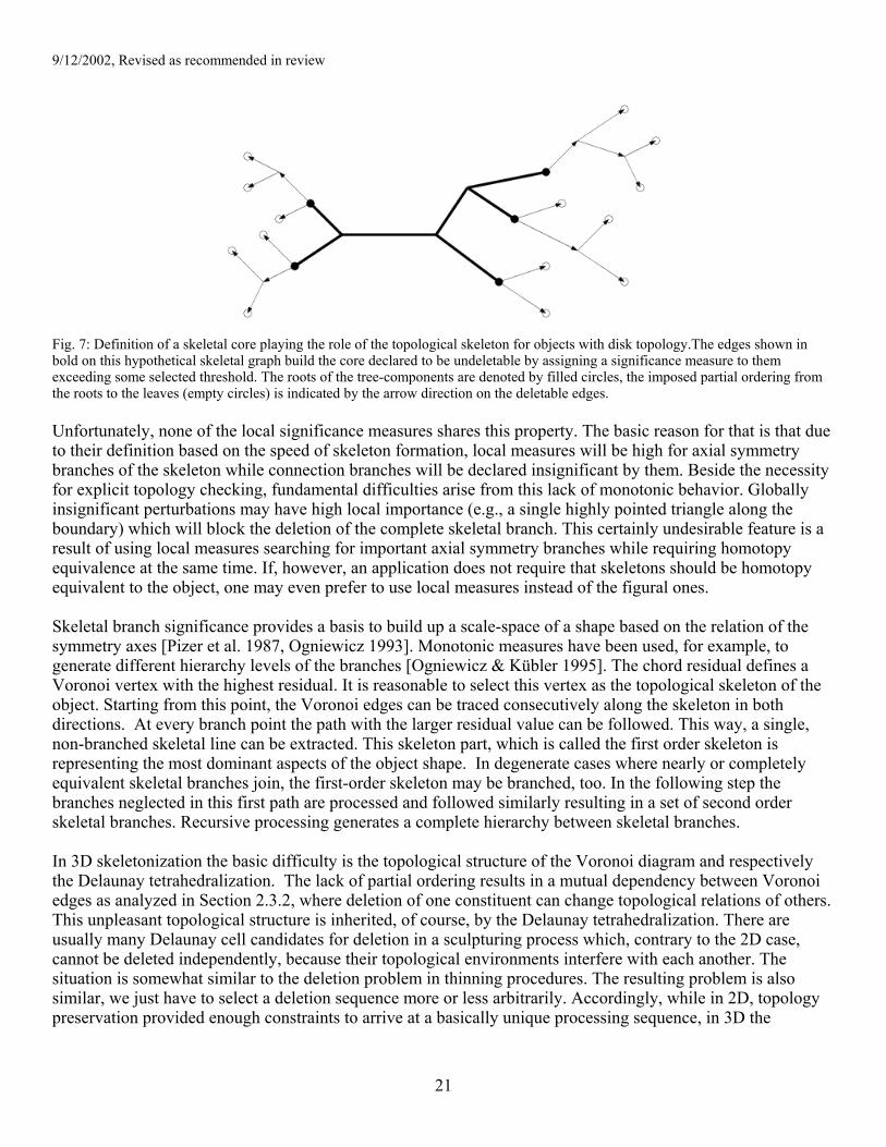
Fig. 7: Definition of a skeletal core playing the role of the topological skeleton for objects with disk topology.The edges shown in bold on this hypothetical skeletal graph build the core declared to be undeletable by assigning a significance measure to them exceeding some selected threshold. The roots of the tree-components are denoted by filled circles, the imposed partial ordering from the roots to the leaves (empty circles) is indicated by the arrow direction on the deletable edges. Unfortunately, none of the local significance measures shares this property. The basic reason for that is that due to their definition based on the speed of skeleton formation, local measures will be high for axial symmetry branches of the skeleton while connection branches will be declared insignificant by them. Beside the necessity for explicit topology checking, fundamental difficulties arise from this lack of monotonic behavior. Globally insignificant perturbations may have high local importance (e.g., a single highly pointed triangle along the boundary) which will block the deletion of the complete skeletal branch. This certainly undesirable feature is a result of using local measures searching for important axial symmetry branches while requiring homotopy equivalence at the same time. If, however, an application does not require that skeletons should be homotopy equivalent to the object, one may even prefer to use local measures instead of the figural ones. Skeletal branch significance provides a basis to build up a scale-space of a shape based on the relation of the symmetry axes [Pizer et al. 1987, Ogniewicz 1993]. Monotonic measures have been used, for example, to generate different hierarchy levels of the branches [Ogniewicz & Kübler 1995]. The chord residual defines a Voronoi vertex with the highest residual. It is reasonable to select this vertex as the topological skeleton of the object. Starting from this point, the Voronoi edges can be traced consecutively along the skeleton in both directions. At every branch point the path with the larger residual value can be followed. This way, a single, non-branched skeletal line can be extracted. This skeleton part, which is called the first order skeleton is representing the most dominant aspects of the object shape. In degenerate cases where nearly or completely equivalent skeletal branches join, the first-order skeleton may be branched, too. In the following step the branches neglected in this first path are processed and followed similarly resulting in a set of second order skeletal branches. Recursive processing generates a complete hierarchy between skeletal branches. In 3D skeletonization the basic difficulty is the topological structure of the Voronoi diagram and respectively the Delaunay tetrahedralization. The lack of partial ordering results in a mutual dependency between Voronoi edges as analyzed in Section 2.3.2, where deletion of one constituent can change topological relations of others. This unpleasant topological structure is inherited, of course, by the Delaunay tetrahedralization. There are usually many Delaunay cell candidates for deletion in a sculpturing process which, contrary to the 2D case, cannot be deleted independently, because their topological environments interfere with each another. The situation is somewhat similar to the deletion problem in thinning procedures. The resulting problem is also similar, we just have to select a deletion sequence more or less arbitrarily. Accordingly, while in 2D, topology preservation provided enough constraints to arrive at a basically unique processing sequence, in 3D the
21
9/12/2002, Revised as recommended in review
homotopy condition seems to be insufficient, i.e., topology is too weak to constrain the problem. Thus we face in 3D an underconstrained problem, leading to multiple solutions. One can try to add additional constraints in order to arrive at a unique solution, but no natural way has been found to define them. 4.3. Shock loci : a Hamilton-Jacobi formulation Shock-capturing numerical methods based on level set techniques can be used to simulate the curve/surface grassfire evolution, but these have the limitation that the shocks, which coincide with medial axis positions, are not explicitly detected. As mentioned earlier, interpolation strategies have been used in 2D to locate the shocks using differential properties of the embedding surface, but the computational complexity of such approaches can be extremely high. More seriously, it is not clear how to guarantee that the topology of the object is preserved, and extensions to 3D are not immediate. See Arcelli et al. [1981] and Arcelli & Baja [1992]. The Hamilton-Jacobi formulation provides a natural way of distinguishing medial points from non-medial ones and effectively addresses several of the above issues. The key idea is to compute a measure of the average outward flux of the vector field q&r . Strictly speaking, the average outward flux is desired only in the limit as the region shrinks to a point. However, the average outward flux over a very small neighborhood (in practice a circle in 2D or a sphere in 3D) will provide a sufficient approximation to the limiting values that distinguish medial from non-medial points. This, being an integral formulation, is much less sensitive to small perturbations than derivative based computations. The average outward flux calculation is an effective way of detecting strong singularities where the vector field's direction changes rapidly around a small neighborhood, i.e., points on the medial locus. However, this calculation is not by itself sufficient to yield topologically correct skeletons that can be interpreted as graphs, an advantage that the Voronoi method has in 2D. One way to solve this problem is to incorporate a homotopy preserving thinning process, where the removal of points is guided by their outward flux values. We defer this discussion to Section 5.2, where we shall develop a computer algorithm, characterize its efficiency, and present illustrative 2D and 3D examples. 4.4. Cores Many mathematical properties of the core derive from generic properties of height ridge, height saddles, and partial critical loci of a function f of values in ℜn. Others derive from the form of the medialness function M. While maximum convexity d-dimensional height ridges on generic functions can be shown generically not to branch, they do end. Ends occur when in some direction in the subspace of maximization f flattens and turns to becoming a minimum, thus transforming in to d-dimensional height saddles. These in turn can lose another dimension of positive second derivative or they can turn back into height ridges. Relative critical sets, and in particular, height saddles can intersect each other and can intersect height ridges. When they do so, generically it is at critical points of M and they intersect transversely and thus cross each other. This all has relevance for maximum convexity cores. Damon and Miller have studied these cores for medialness functions that are functions of position x and medial width r but are constant with respect to the medial frame and object angle, such as M(x,r)= ∇2G(x,kr) * I(x), where I is the target image and G(x,kr) is a zero mean Gaussian with standard deviation kr for some constant k. For such medialness functions the maximum convexity cores, which by definition are maximum convexity ridges, will not generically branch, but at an object branch at least one of the branches changes from a height ridge to a height saddle, and then the two height saddle curves or one height saddle and one height ridge cross at the branch point.
22

9/12/2002, Revised as recommended in review
Optimal parameter cores differ in two ways from the scenario just described. First, they are a plied o medialness functions M(x
p t,p) that are multilocal, i.e., they are functions of the medial frame ( )⊥bbnx
rrr ,, and the object angle θ, for example by summing boundary strength at the end of each of the medial sails in the direction of the sails. Second, they involve maximization with respect to a direction within x of medialness restricted to the n-3-dimensional ridge made from the initial optimization of medialness over p, which includes medial width, medial frame, and object angle. Optimal parameter cores on multilocal medialness functions have different generic properties with respect to branching, crossing, and ending. At branch points they can and typically do stay as three height ridges that generically do not cross at a single point in x, let alone in x, r (see Fig. 8). And when two height ridges cross at a particular value of x, they typically do not agree in r, nor the medial frame, nor the object angle, and thus they do not agree in medialness value.
Fig. 8. Positional core loci at a branching bar. Courtesy of Yoni Fridman. Second, differences in ending of optimal parameter cores arise at singularities of the projection of the n-3-dimensional ridge made from optimizing medialness over p. In the case of only scale as a parameter (with medialness functions that are not multilocal), the height ridges continue transversely through the fold singular points, changing to height saddles [Miller 1998]. For multiple parameters p, this behavior should remain unchanged. Cusps, which are higher order singularities of the projection, can occur in an ambient space of dimension 2 or higher, but only for an ambient space of dimension 3 or higher will the 2D ridge generically encounter this cusp. For yet higher order singularities, such as swallowtails, which can occur only in an ambient space of dimension 3 or higher, the behavior has not been determined. Maximum convexity cores on multilocal medialness functions still cannot branch or cross, but at an object branch after some of the ridges change into height saddles of medialness, they can cross. After such crossings frequently the relative critical set, whether as a height saddle or reforming as a height ridge, continues past the branch to approximately bisect the other two branches, in a way roughly like that in Fig. 8. The major strength of cores is that they can be applied not just to binary images, derivable from boundaries, but also to greyscale images. However, because cores, of either type, neither end only at places where an object ends but also where the contrast of the object gets appropriately low relative to the intensity noise, a special test for ends is needed, e.g., by testing for a maximum of a different function that we call endness in the d dimensions of the height ridge. At places which fail this test, frequently the height saddle soon changes back into a height ridge, and the medial locus can be taken as the union of the height ridge and the height saddle.
23
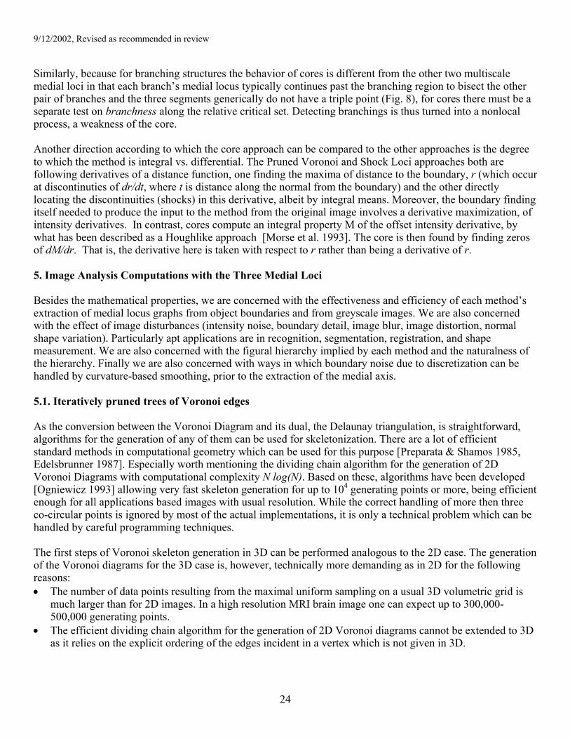
9/12/2002, Revised as recommended in review
Similarly, because for branching structures the behavior of cores is different from the other two multiscale medial loci in that each branch’s medial locus typically continues past the branching region to bisect the other pair of branches and the three segments generically do not have a triple point (Fig. 8), for cores there must be a separate test on branchness along the relative critical set. Detecting branchings is thus turned into a nonlocal process, a weakness of the core. Another direction according to which the core approach can be compared to the other approaches is the degree to which the method is integral vs. differential. The Pruned Voronoi and Shock Loci approaches both are following derivatives of a distance function, one finding the maxima of distance to the boundary, r (which occur at discontinuties of dr/dt, where t is distance along the normal from the boundary) and the other directly locating the discontinuities (shocks) in this derivative, albeit by integral means. Moreover, the boundary finding itself needed to produce the input to the method from the original image involves a derivative maximization, of intensity derivatives. In contrast, cores compute an integral property M of the offset intensity derivative, by what has been described as a Houghlike approach [Morse et al. 1993]. The core is then found by finding zeros of dM/dr. That is, the derivative here is taken with respect to r rather than being a derivative of r. 5. Image Analysis Computations with the Three Medial Loci Besides the mathematical properties, we are concerned with the effectiveness and efficiency of each method’s extraction of medial locus graphs from object boundaries and from greyscale images. We are also concerned with the effect of image disturbances (intensity noise, boundary detail, image blur, image distortion, normal shape variation). Particularly apt applications are in recognition, segmentation, registration, and shape measurement. We are also concerned with the figural hierarchy implied by each method and the naturalness of the hierarchy. Finally we are also concerned with ways in which boundary noise due to discretization can be handled by curvature-based smoothing, prior to the extraction of the medial axis. 5.1. Iteratively pruned trees of Voronoi edges As the conversion between the Voronoi Diagram and its dual, the Delaunay triangulation, is straightforward, algorithms for the generation of any of them can be used for skeletonization. There are a lot of efficient standard methods in computational geometry which can be used for this purpose [Preparata & Shamos 1985, Edelsbrunner 1987]. Especially worth mentioning the dividing chain algorithm for the generation of 2D Voronoi Diagrams with computational complexity N log(N). Based on these, algorithms have been developed [Ogniewicz 1993] allowing very fast skeleton generation for up to 104 generating points or more, being efficient enough for all applications based images with usual resolution. While the correct handling of more then three co-circular points is ignored by most of the actual implementations, it is only a technical problem which can be handled by careful programming techniques. The first steps of Voronoi skeleton generation in 3D can be performed analogous to the 2D case. The generation of the Voronoi diagrams for the 3D case is, however, technically more demanding as in 2D for the following reasons: • The number of data points resulting from the maximal uniform sampling on a usual 3D volumetric grid is
much larger than for 2D images. In a high resolution MRI brain image one can expect up to 300,000-500,000 generating points.
• The efficient dividing chain algorithm for the generation of 2D Voronoi diagrams cannot be extended to 3D as it relies on the explicit ordering of the edges incident in a vertex which is not given in 3D.
24
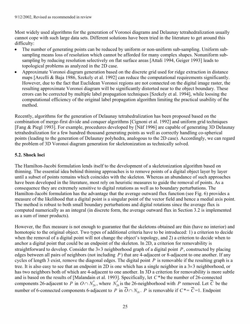
9/12/2002, Revised as recommended in review
Most widely used algorithms for the generation of Voronoi diagrams and Delaunay tetrahedralization usually cannot cope with such large data sets. Different solutions have been tried in the literature to get around this difficulty: • The number of generating points can be reduced by uniform or non-uniform sub-sampling. Uniform sub-
sampling means loss of resolution which cannot be afforded for many complex shapes. Nonuniform sub-sampling by reducing resolution selectively on flat surface areas [Attali 1994, Geiger 1993] leads to topological problems as analyzed in the 2D case.
• Approximate Voronoi diagram generation based on the discrete grid used for ridge extraction in distance maps [Arcelli & Baja 1986, Szekely et al. 1992] can reduce the computational requirements significantly. However, due to the fact that Euclidean Voronoi regions are not connected on the digital image raster, the resulting approximate Voronoi diagram will be significantly distorted near to the object boundary. These errors can be corrected by multiple label propagation techniques [Szekely et al. 1994], while loosing the computational efficiency of the original label propagation algorithm limiting the practical usability of the method.
Recently, algorithms for the generation of Delaunay tetrahedralization has been proposed based on the combination of merge-first divide and conquer algorithms [Cignoni et al. 1992] and uniform grid techniques [Fang & Piegl 1993]. For example, procedures developed by [Näf 1996] are capable of generating 3D Delaunay tetrahedralization for a few hundred thousand generating points as well as correctly handling co-spherical points (leading to the generation of Delaunay polyhedra, analogous to the 2D case). Accordingly, we can regard the problem of 3D Voronoi diagram generation for skeletonization as technically solved. 5.2. Shock loci The Hamilton-Jacobi formulation lends itself to the development of a skeletonization algorithm based on thinning. The essential idea behind thinning approaches is to remove points of a digital object layer by layer until a subset of points remains which coincides with the skeleton. Whereas an abundance of such approaches have been developed in the literature, most rely on heuristic measures to guide the removal of points. As a consequence they are extremely sensitive to digital rotations as well as to boundary perturbations. The Hamilton-Jacobi formulation has the advantage that the average outward flux function (see Fig. 6) provides a measure of the likelihood that a digital point is a singular point of the vector field and hence a medial axis point. The method is robust to both small boundary perturbations and digital rotations since the average flux is computed numerically as an integral (in discrete form, the average outward flux in Section 3.2 is implemented as a sum of inner products). However, the flux measure is not enough to guarantee that the skeletons obtained are thin (have no interior) and homotopic to the original object. Two types of additional criteria have to be introduced: 1) a criterion to decide when the removal of a digital point will not change the object’s topology, and 2) a criterion to decide when to anchor a digital point that could be an endpoint of the skeleton. In 2D, a criterion for removability is straightforward to develop. Consider the 3×3 neighborhood graph of a digital point P , constructed by placing edges between all pairs of neighbors (not including P ) that are 4-adjacent or 8-adjacent to one another. If any cycles of length 3 exist, remove the diagonal edges. The digital point P is removable if the resulting graph is a tree. It is also easy to see that an endpoint in 2D is one which has a single neighbor in a 3×3 neighborhood, or has two neighbors both of which are 4-adjacent to one another. In 3D a criterion for removability is more subtle and is based on the results of [Malandain et al. 1993]. Specifically, let C *be the number of 26-connected components 26-adjacent to P in O , where is the 26-neighborhood with ∩ N26
* N26* P removed. Let C be the
number of 6-connected components 6-adjacent to P in O ∩ N18 . P is removable if C *= C =1. Endpoint
25
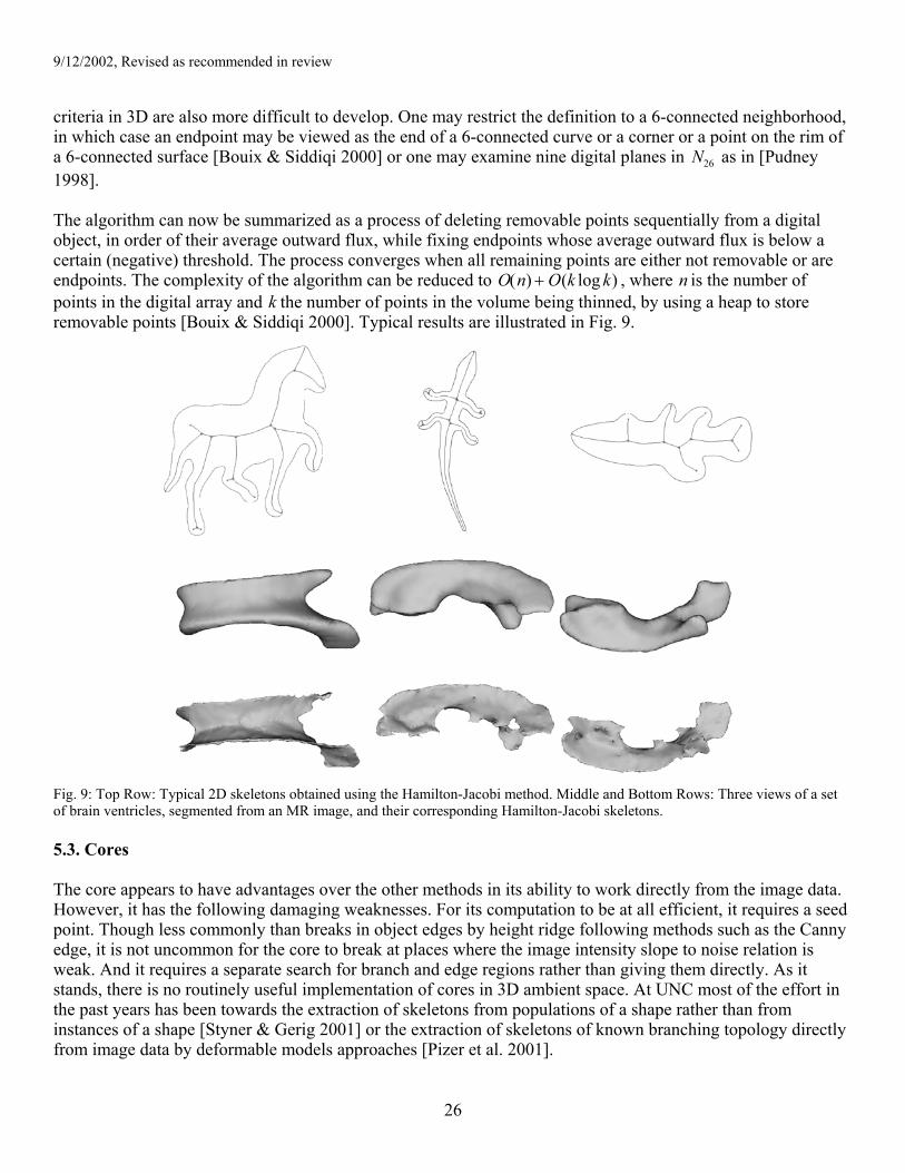
9/12/2002, Revised as recommended in review
criteria in 3D are also more difficult to develop. One may restrict the definition to a 6-connected neighborhood, in which case an endpoint may be viewed as the end of a 6-connected curve or a corner or a point on the rim of a 6-connected surface [Bouix & Siddiqi 2000] or one may examine nine digital planes in N26 as in [Pudney 1998]. The algorithm can now be summarized as a process of deleting removable points sequentially from a digital object, in order of their average outward flux, while fixing endpoints whose average outward flux is below a certain (negative) threshold. The process converges when all remaining points are either not removable or are endpoints. The complexity of the algorithm can be reduced to O(n) + O(k log k) , where n is the number of points in the digital array and k the number of points in the volume being thinned, by using a heap to store removable points [Bouix & Siddiqi 2000]. Typical results are illustrated in Fig. 9.
Fig. 9: Top Row: Typical 2D skeletons obtained using the Hamilton-Jacobi method. Middle and Bottom Rows: Three views of a set of brain ventricles, segmented from an MR image, and their corresponding Hamilton-Jacobi skeletons. 5.3. Cores The core appears to have advantages over the other methods in its ability to work directly from the image data. However, it has the following damaging weaknesses. For its computation to be at all efficient, it requires a seed point. Though less commonly than breaks in object edges by height ridge following methods such as the Canny edge, it is not uncommon for the core to break at places where the image intensity slope to noise relation is weak. And it requires a separate search for branch and edge regions rather than giving them directly. As it stands, there is no routinely useful implementation of cores in 3D ambient space. At UNC most of the effort in the past years has been towards the extraction of skeletons from populations of a shape rather than from instances of a shape [Styner & Gerig 2001] or the extraction of skeletons of known branching topology directly from image data by deformable models approaches [Pizer et al. 2001].
26
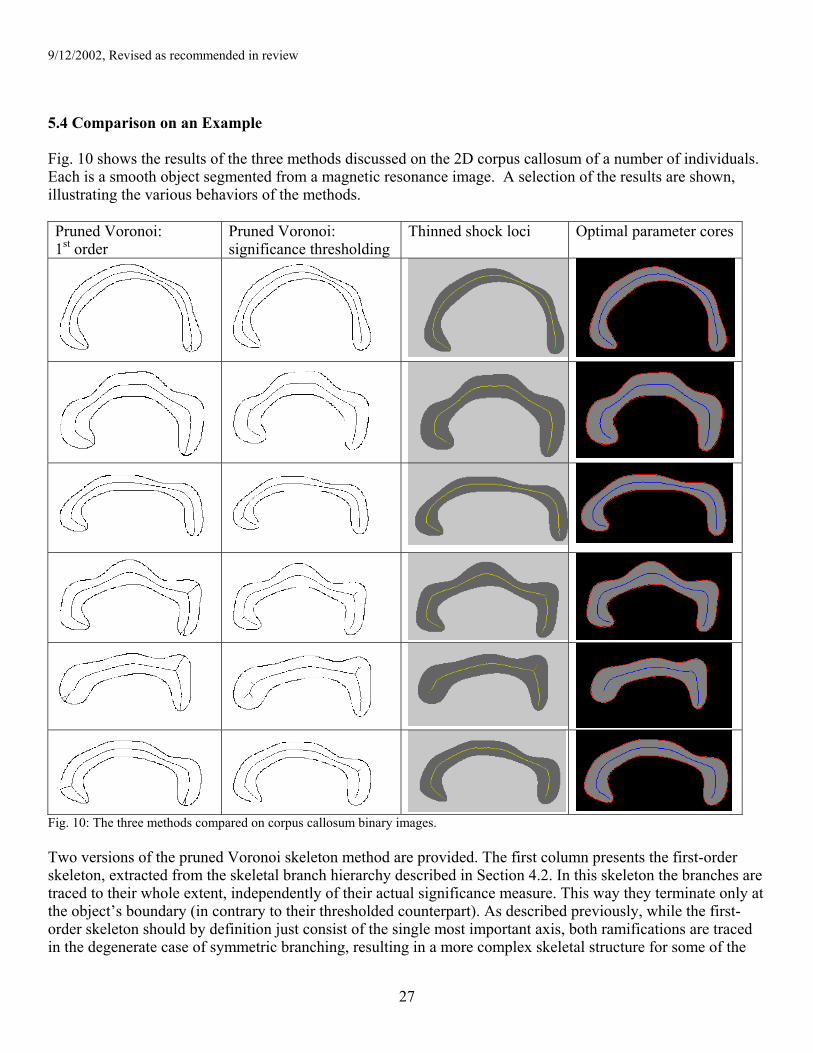
9/12/2002, Revised as recommended in review
5.4 Comparison on an Example Fig. 10 shows the results of the three methods discussed on the 2D corpus callosum of a number of individuals. Each is a smooth object segmented from a magnetic resonance image. A selection of the results are shown, illustrating the various behaviors of the methods. Pruned Voronoi: 1st order
Pruned Voronoi: significance thresholding
Thinned shock loci Optimal parameter cores
Fig. 10: The three methods compared on corpus callosum binary images. Two versions of the pruned Voronoi skeleton method are provided. The first column presents the first-order skeleton, extracted from the skeletal branch hierarchy described in Section 4.2. In this skeleton the branches are traced to their whole extent, independently of their actual significance measure. This way they terminate only at the object’s boundary (in contrary to their thresholded counterpart). As described previously, while the first-order skeleton should by definition just consist of the single most important axis, both ramifications are traced in the degenerate case of symmetric branching, resulting in a more complex skeletal structure for some of the
27
9/12/2002, Revised as recommended in review
presented examples. In the second column the result of the simple thresholding process is shown, using a figural significance measure, namely the chord residual mentioned in Section 4.2. Simple heuristics have been used for the selection of the actual threshold value, so as to rid branches induced by boundary discretization artifacts. In some cases (e.g., row 2 in Fig. 10) these results in the second column produce small branches not appearing in the thinned shock loci results. The core results were produced by hand initializing a core internal to the object and following the medialness ridge. On that ridge a measure of end strength and a measure of branch strength was computed. The core was terminated at a strong maximum of the measure of end strength, and branches were initialized at locations where the branch strength was appropriately high. However, the measures of end strength are both still in an intermediate stage of research [Fridman 2002], and the measure of branch strength is at present designed only to detect branches that produce a strong concavity (hyperbolicity in 3D), a property achieved with tubular trees but not in these corpora callosa. As a result, in contrast to the other two methods, the present core results show no branches. Except for that difference, all three methods achieve reasonable medial loci and somewhat comparable results. The thinned shock loci results show as intensity the average divergence level that serves as a medial strength in this method. In general, at the present stage of development of each of the three methods, the thinned shock loci method produces the best combination of branching and ending performance of the three methods. 6. Summary & Conclusion In this paper we faced both mathematical and computational issues in regard to methods for extracting medial loci from either boundaries of objects or from greyscale images of these objects. We found that because of their basis in differing approximations, the three loci were not the same and have different crossing, branching, and ending behaviors. A subset of the Voronoi and shock loci both converge in the limit to the Blum medial locus. In contrast, cores converge in the limit to a different subset of the symmetry set. Today, from a practical point of view the authors agree that in 2D the problem of extraction of skeletons from individual smooth boundaries is solved and there is not much space left for additional research work, except towards increased speed. In 3D the methods discussed provide a variety of ways to generate medial loci which work robustly enough in many cases for shape description and object modeling applications. The method of choice will depend on the application. However, in test cases with complex branching, complex topology, near nongeneric states, or considerable levels of boundary noise, none of the presently available methods in 2D or 3D meets the test of combining mathematical agreement of branching and topological structure and the production of an intuitively reasonable branching structure. From a mathematical viewpoint, it is possible to find methods that stably extract medial loci given known limits on the scale of the boundary description, e.g., the length of linear segments or the size of pixels or voxels making up a boundary point list. However, especially in 3D, despite the frequent success of the multiscale methods that have been discussed in this paper, when we start from boundaries including aspects at smaller than the criterion scale, we frequently cannot achieve fully satisfactory computation of the medial locus and its branching structure. The fundamentally unsolved issue is the selection of a subset of detected symmetries that is meaningful to a particular application and that yields stability against changes in the boundary that seem perceptually small. This problem can be seen in terms of two related questions: how to increase scale and how to generate the branching structure. Apart from simple considerations to get rid of primary noise branches directly caused by the digital approximation of the continuous boundary [Ogniewicz
28

9/12/2002, Revised as recommended in review
1993], we do not know how to choose pruning thresholds for the pruned Voronoi approach. We do not know how to choose the amount of smoothing of the Euclidean distance function in the curve/surface evolution method. And we do not know how to choose the factor relating medial radius to the aperture at which the image is sensed and how to generate a correct branching structure in the core method. Acknowledgments We gratefully acknowldege the contributions of Delphine Bull, Sylvain Bouix, P. Thomas Fletcher, Yonatan Fridman, Jacob Furst, Andrew Thall, and Paul Yushkevich to this paper. We thank Guido Gerig for the corpus callosum data used in Fig. 10. The work reported in this paper was partially supported by NIH grant P01 CA47982, NSF grant DMS 0103862, NSERC Canada, FCAR Quebec and Swiss National Science Foundation Grant 2-77-938-94. SZ grants. AFOSR and DARPA. References Arcelli, C, LP Cordella, S Leviadi (1981). From Local Maxima to Connected Skeletons. IEEE Transactions on
Pattern Analysis and Machine Intelligence, 3(2): 134-143. Arcelli, C & G Sanniti di Baja (1986). Computing Voronoi diagrams in digital pictures, Pattern Rec. Letters.
4(5): 383-389. Arcelli, C & Gabriela Sanniti di Baja (1992). Ridge Points in Euclidean Distance Maps. Pattern Recognition
Letters, 13(4): 237-243. Asada, H & M Brady (1986). The curvature primal sketch. IEEE PAMI 8: 2-14. Attali, D (1995). Squelettes et graphes de Voronoi 2D et 3D, PhD thesis, Université Joseph Fourier, Grenoble. Attali, D, P Bertolino, A Montanvert (1994). Using polyballs to approximate shapes and skeletons. Proc. 12th
Int. Conf. Pattern Recogn.: 626-628. Attali, D & A Montanvert (1994). Semicontinuous skeletons of 2d and 3d shapes. In C Arcelli, LP Cordella,
and G Sanniti di Baja, Eds. Aspects of Visual Form Processing: 32-41, World Scientific. Attneave, F (1954). Some informational aspects of visual perception, Psychol. Rev. 61: 183-193. August, J, A Tannenbaum, S Zucker (1999a). On the evolution of the skeleton. ICCV’99: 315-322, Kerkyra,
Greece, IEEE. August, J, K Siddiqi, SW Zucker (1999b). Ligature instabilities in the perceptual organization of shape.
Computer Vision and Image Understanding, 76: 231- 243. August, J, K Siddiqi, SW Zucker (1999c). Contour Fragment Grouping and Shared, Simple Occluders.
Computer Vision and Image Understanding, 76(2): 146-162. Biederman, I (1987). Recognition by components. Psychological Review 94: 115-147. Blum, H (1967). A transformation for extracting new descriptors of shape. In W Wathen-Dunn, ed., Models for
the Perception of Speech and Visual Form. MIT Press, Cambridge, MA: 363-380. Blum, H (1973). Biological Shape and Visual Science. Journal Theor. Biol., 38: 205-287. Blum, H & RN Nagel (1978). Shape description using weighted symmetric axis features. Pattern Recognition,
10: 167-180. Bogaevski, IA (1990), Modifications of singularities of minimum functions and bifurcations of shock waves of
the Burger's equation with vanishing viscosity, Leningrad Math. J.1: 807-823. Bouix, S & K Siddiqi (2000). Divergence-based medial surfaces. In ECCV’2000: 603-618, Dublin, Ireland,
IEEE. Brady, M & H Asada (1984). Smoothed Local Symmetries and Their Implementation. International Journal of
Robotics Research, 3(3): 36-61.
29
9/12/2002, Revised as recommended in review
Brandt, JW (1992). Describing a solid with three-dimensional skeleton, in Curves and Surfaces in Comp. Vision and Graphics III, SPIE, 1830:258-269.
Brandt, JW & VR Algazi (1992). Continuous skeleton computation by Voronoi diagram, Comp. Vis. Graphics Image Proc.: Image Understanding 55(3):329-338.
Brockett, R, P Maragos (1992). Evolution equations for continuous-scale morphology. Proc. IEEE Conference on Acoustics, Speech and Signal Processing.
Bruce, JW, PJ Giblin, C Gibson (1985). Symmetry sets. Proc. Roy. Soc. Edinburgh 101A:163-186. Bruce, JW & PJ Giblin (1986). Growth, motion, and 1-parameter families of symmetry sets. Proc. Roy. Soc.
Edinburgh 104A:163-186. Bruce, JW, PJ Giblin, F Tari (1996). Ridges, crests and sub-parabolic lines of evolving surfaces. Int. J.
Computer Vision. 18:195-210. Burbeck, C & S Hadden (1993). Scaled Position Integration Areas: Accounting for Weber's law for separation.
Journal of the Optical Society of America, 10(1): 5-15. Burbeck, CA & SM Pizer(1995). Object Representation by Cores: Identifying and Representing Primitive
Spatial Regions. Vision Research, 35: 1917-1930. Burbeck, CA, SM Pizer, BS Morse, D Ariely, GS Zauberman, J Rolland (1996). Linking Object Boundaries at
Scale: A Common Mechanism for Size and Shape Judgements. Vision Research, 36:361-372. Cignoni, P, C Montani, R Scopigno (1992). A merge-first divide and conquer algorithm for ed Delaunay
triangulation, Technical report, CNUCE. Cross, ADJ & E Hancock (1997). Scale-space vector fields for feature analysis. CVPR: 738 – 743, IEEE. Culver, T, J Keyser, D Manocha (1999). Accurate computation of the medial axis of a polyhedron. Proc. 5th
Symp. Solid Modeling and Appl.: 179-204. Culver, T (2000). Computing the medial axis of a polyhedron. PhD dissertation, Dept. of Comp. Sci., Univ. of
NC. Also see website www.cs.unc.edu/~culver/diss. Damon, J (1999). Properties of ridges and cores for two-dimensional images (2D height ridges and connectors).
J. Math. Imag. & Vision, 10:163-174. Damon, J (1998). Generic structure of two-dimensional images under Gaussian blurring (2D height ridges and
connectors – full math). SIAM J. Appl. Math. 59:97-138. Damon, J (1997). Singularities with scale threshold and discrete functions exhibiting generic properties.
Matemática Contemporânea, 12:45-65. Dimitrov, P, Phillips, C & Siddiqi, K (2000). Robust and efficient skeletal graphs. CVPR’2000:1:417-423,
Hilton Head, SC, IEEE. Eberly, D (1996). Ridges in Image and Data Analysis. Series on Computational Imaging and Vision. Kluwer
Academic Publishers, Dordrecht, The Netherlands . Edelsbrunner H (1987). Algorithms in Combinatorial Geometry, Monographs on Theoretical Computer
Science. 10, Springer-Verlag. Elder, J & S Zucker (1993). The Effect of Contour Closure on the Rapid Discrimination of Two-Dimensional
Shapes. Vision Research, 33(7): 981-991, 1993 Fang, TP & LA Piegl (1993). Delaunay triangulation using a uniform grid, IEEE Computer Graphics and
Applications. 13(3):36-47. Fritsch, DS, SM Pizer, B Morse, DH Eberly, A Liu (1994). The multiscale medial axis and its applications in
image registration. Pattern Recognition Letters, 15:445-452. Furst, JD, RS Keller, JE Miller, SM Pizer (1997). Image loci are ridges in geometric Spaces. Scale-Space
Theory in Computer Vision: Proceedings of First International Conference, BM ter Haar Romeny, ed. Springer Lecture Notes in Computer Science 1252:176-187, Springer-Verlag, Berlin.
Furst, JD and SM Pizer (2001). Marching Ridges. IASTED International Conference on Signal and Image Processing: 22-26.
30

9/12/2002, Revised as recommended in review
Geiger, B (1993). Three-dimensional modeling of human organs and its application to diagnostic and surgical planning, Technical Report RR-2105, INRIA.
Giblin, P, B Kimia (1999). On the local form and transitions of symmetry sets, medial axes, and shocks. Proc. of the 7th International Conference on Computer Vision, ICCV ’99: 385-391.
Giblin, P, B Kimia (2000). A formal classification of 3D medial axis points and their local geometry. Proc. CVPR 2000, 11: 566-573, IEEE.
Giblin, P & B Kimia (2002). Transitions of the 3D Medial Axis under a one-parameter family of deformations. Proc. ECCV 2002: 718 – 734, IEEE.
Gomez, J & O Faugeras (2000). Level sets and distance functions. Proc. ECCV, 1: 588-602. Held, M (1998). Voronoi diagrams and offset curves of curvilinear polygons. Comput. Aided Design, 30(4):
287-300. Katz, RA & SM Pizer (2001). Untangling the Blum medial axis transform. Int. J. Comp. Vis., this issue. Keller, R (1999). Generic transitions of relative critical sets in parametrized families with applications to image
analysis. PhD dissertation, Dept. of Math., Univ. of NC. Kimmel, R, D Shaked, N Kiryati (1995). Skeletonization via distance maps and level sets. CVIU, 62(3): 382-
391. Kimia B, A Tannenbaum, SW Zucker (1990). Toward a computational theory of shape: An overview, Proc.
First European Conf. on Computer Vision, O. Faugeras, ed. Lecture Notes in Computer Science, 427, Springer Verlag, New York.
Kimia, BB, A Tannenbaum, S Zucker (1995). Shape, shocks, and deformations {I}: The components of two-dimensional shape and the reaction-diffusion space. International Journal of Computer Vision, 15:189-
224. Klein, F (1987). Euclidean skeletons. Proc. 5th Scandinavian Conf. Image Anal., 443-450. Koenderink, JJ. (1990). Solid Shape. MIT Press, Cambridge, MA. Lax, PD (1971). Shock waves and entropy. Contributions to Nonlinear Functional Analysis, 603-634,
Academic Press. Lee, DT (1982). Medial axis transformation of a planar shape. IEEE Trans. Pattern Anal. Mach. Intell., PAMI-
4(4): 363-369. Lee, TS (1996). Neurophysiological Evidence For Image Segmentation And Medial Axis Computation in
Primate V1. Computation and Neural Systems: Proceedings of the Fourth Annual Computational Neuroscience Conference.
Leymarie, F & MD Levine (1992). Simulating the grassfire transform using an active contour model. IEEE Trans. PAMI, 14(1): 56-75.
Leyton, M (1987). Symmetry-curvature duality. Comp. Vision, Graphics, and Image Processing. 38: 327-341. Liu, TL & D Geiger (1999). Approximate tree matching and shape similarity. Proc ICCV: 456 - 461. Malandain, G, Bertrand G & Ayache, N (1993). Topological segmentation of discrete surfaces. International
Journal of Computer Vision. 10(2):183-197. Marr, D & K Nishihara (1978). Representation and recognition of the spatial organization of three dimensional
structure. Proceedings of the Royal Society of London, B 200:269-294. Mather, J (1983). Distance from a manifold in Euclidean space. Proc. Symp. Pure Math. 40(Pt 2):199-216. Matheron, G (1988). Examples of Topological Properties of Skeletons. Image Analysis and Mathematical
Morpholpogy, Part II: Theoretical Advances. 217-238, Academic Press. Meyer, F (1989). Skeletons and perceptual graphs, Signal Processing. 16: 335-363. Miller, J (1998). Relative critical sets in ℜn and applications to image analysis. PhD dissertation, Dept. of
Math., Univ. of NC.
31

9/12/2002, Revised as recommended in review
Miller, J & JD Furst (1999). The maximal scale ridge: incorporating scale into the ridge definition. Scale-Space Theories in Computer Vision: Proceedings of Second International Conference, M Nielsen, P Johansen, O Fogh Olsen, J Weickert, eds. Springer Lecture Notes in Computer Science, 1682: 93-104
Morse BS, SM Pizer, A Liu (1993). Multiscale medial analysis of medical images. Information Processing in Medical Imaging (IPMI '93), Barrett, H. H., Gmitro, A. F., eds. Lecture Notes in Computer Science, 687: 112-131, Springer-Verlag. In revised form in Image & Vision Computing, 12: 327-338.
Morse BS, SM Pizer, DT Puff, C Gu (1998). Zoom-Invariant Vision of Figural Shape: Effects on Cores of Image Disturbances. Computer Vision and Image Understanding, 69: 72-86.
Nackman, LR (1981). Three-dimensional shape description using the symmetric axis transform. PhD dissertation, Dept. of Comp. Sci., Univ of NC.
Nackman, LR & SM Pizer (1985). Three-dimensional shape description using the symmetric axis transform, I: Theory. IEEE Trans. PAMI, 7(2): 187-202.
Näf, M (1996). 3D Voronoi Skeletons: a semicontinuous implementation of the 'Symmetric Axis Transform' in 3D space, PhD thesis ETH Zürich.
Ogniewicz, RL (1993). Discrete Voronoi Skeletons, Hartung-Gorre Verlag. Ogniewicz, RL & O.Kübler (1995). Hierarchic voronoi skeletons, Pattern Recognition. 28: 343-359. Osher, S & J Sethian (1988). Fronts propagating with curvature dependent speed: Algorithms based on
Hamilton-Jacobi formulations. Journal of Computational Physics, 79: 12-49. Pelillo, M, K Siddiqi, S Zucker (1998). Matching Hierarchical Structures Using Association Graphs.
Proceedings of the European Conference on Computer Vision. Pizer, SM, WR Oliver, SH Bloomberg (1987). Hierarchical shape description via the multiresolution symmetry
axis transform. IEEE PAMI. 9(4): 505-511. Pizer, SM, DS Fritsch, V Johnson, EL Chaney (1996). Segmentation, registration and measurement of shape
variation via image object shape. IEEE TMI. 18(10): 851-865. Pizer, SM, D Eberly, BS Morse, DS Fritsch (1998). Zoom-Invariant Figural Shape: The Mathematics of Cores.
Computer Vision and Image Understanding (CVIU '98) 69: 55-71. Pizer, SM, JZ Chen, PT Fletcher, Y Fridman, DS Fritsch, AG Gash, JM Glotzer, MR Jiroutek, S Joshi, C Lu,
KE Muller, A Thall, G Tracton, P Yushkevich, EL Chaney (2001). Deformable m-Reps for 3D medical image segmentation. Submitted for publication in this issue.
Preparata, FP & MI Shamos (1985). Computational Geometry, Springer-Verlag. Pudney, C (1998). Distance-ordered homotopic thinning: A skeletonization algorithm for 3d digital images. Computer Vision and Image Understanding (CVIU '98) 72(3): 404-413. Rom, H & G Medioni (1993). Hierarchical Decomposition And Axial Shape Description. IEEE Transactions on
Pattern Analysis and Machine Intelligence, 15(10): 973-981. Romeny, B (1994). Geometry-Driven Diffusion in Computer Vision. Computational Imaging and Vision,
Kluwer Academic Publishers. Schmitt, M (1989). Some examples of algorithms analysis in computational geometry by means of
mathematical morphological techniques, In J.D. Boissonnat and J.P. Laumons, Eds., Geometry and robotics, Lecture Notes in Computer Science, 291: 225-246, Springer-Verlag.
Sclaroff, S (1997). Deformable Prototypes for Encoding Shape Categories in Image Databases. Pattern Recognition, 30(4).
Sebastian, TB, PN Klein, BB Kimia (2001). Recognition of shapes by editing shock graphs. Proc. 8th ICCV, IEEE
Serra, J (1982). Image Analysis and Mathematical Morpholpogy. Academic Press. Sethian, JA (1996). Level Set Methods: Evolving Interfaces in Geometry, Fluid Mechanics, Computer Vision,
and Materials Science. Cambridge University Press.
32

9/12/2002, Revised as recommended in review
Shah, J (1996). A common framework for curve evolution, segmentation, and anisotropic diffusion. Proc. of CVPR: 136-142, IEEE.
Sibel, Z, G Tari, J Shah, H Pien (1997). Extraction of Shape Skeletons from Grayscale Images. Computer Vision and Image Understanding.
Siddiqi, K & BB Kimia (1996). A shock grammar for recognition. CVPR’96:507-513, San Francisco, CA, IEEE.
Siddiqi, K, CW Shu, BB Kimia (1997). Geometric shock-capturing ENO schemes for subpixel interpolation, Computation, and Curve Evolution. Graphical Models and Image Processing 59: 278-301.
Siddiqi, K, S Bouix, A Tannenbaum, S Zucker (1999). The Hamilton-Jacobi skeleton. In ICCV’99: 828-834, Kerkyra, Greece, IEEE.
Siddiqi, K, B Kimia, A Tannenbaum, SW Zucker (2001). On the psychophysics of the shape triangle. Vision Research, 41(9): 1153 - 1178.
Siddiqi, K, S Bouix, AR Tannenbaum, SW Zucker (2002). Hamilton-Jacobi Skeletons. Int. Journal of Computer Vision, to appear.
Styner M, & G Gerig (2001). Medial models incorporating object variability for 3D shape analysis. Information Processing in Medical Imaging (IPMI 2001), MF Insana, RM Leahy, eds., Lecture Notes in Computer Science, Springer 2082: 502-516.
Székely, G. (1996). Shape characterization by local symmetries, Habilitation, Swiss Federal Institute of Technology, Zurich.
Székely, G, Ch Brechbühler, O Kübler, RL Ogniewicz, T Budinger, (1992). Mapping the human cerebral cortex using 3d medial manifolds, Proc. 2nd Int. Conf. Visualization in Biomed. Comp, SPIE, 1808: 130-144.
Székely, G, M Näf, Ch Brechbühler, O Kübler (1994). Calculating 3d Voronoi diagrams of large unrestricted point sets for skeleton generation of complex 3d shapes, Proc. 2nd Int. Workshop on Visual Form: 532-541, World Scientific.
Tari, ZS, J Shah, H Pien (1997). Extraction of shape skeletons from grayscale images. CVIU, 66: 133 - 146. Tihonov, AN & V Ya.Arsenin (1977). Solution of ill posed problems, Winston. Weiss, I (1986). Curve fitting with optimal mesh point placement, Technical Report CAR-TR-22, Comp. Vision
Lab. University of Maryland. Weiss, I (1990). Shape reconstruction on a varying mesh, IEEE PAMI, 12(4): 345-362. Whitman, R & DD Hoffman (1985). Codon Constraints on Closed 2D Shapes. CVGIP, 31(2): 265-281. Yomdin, J (1981). On the local structure of the generic central set. Compositio. Math. 43: 225-238. Yu, Z, Ch Conrad, U Eckhardt (1992). Regularization of the medial axis transform, In R.Klette & W.G.
Kropatsch, Eds., Theoretical Foundations of Computer Vision: 13-24. Zhu, S, & AL Yuille (1996). FORMS: a flexible object recognition and modelling system. International
Journal of Computer Vision, 20(3): 187-212.
33