Embed Size (px)
Citation preview

MULTISINE EXCITATION DESIGN TO INCREASE THE EFFICIENCY OF
SYSTEM IDENTIFICATION SIGNAL GENERATION AND ANALYSIS
A DissertationSubmitted to the Graduate Faculty
of theNorth Dakota State University
of Agriculture and Applied Science
By
Michael James Schmitz
In Partial Fulfillment of the Requirementsfor the Degree of
DOCTOR OF PHILOSOPHY
Major Department:Electrical and Computer Engineering
October 2012
Fargo, North Dakota

North Dakota State University
Graduate School
Title
Multisine Excitation Design to Increase the Efficiency of System
Identification Signal Generation and Analysis
By
Michael James Schmitz
The Supervisory Committee certifies that this disquisition complies with North
Dakota State University’s regulations and meets the accepted standards for the
degree of
DOCTOR OF PHILOSOPHY
SUPERVISORY COMMITTEE:
Roger Green
Chair
Rajesh Kavasseri
Daniel Ewert
John Miller
Approved:
10-26-2012
Rajendra Katti
Date
Department Chair

ABSTRACT
Reducing sample frequencies in measurement systems can save power, but reduc-
tion to the point of undersampling results in aliasing and possible signal distortion.
Nonlinearities of the system under test can also lead to distortions prior to mea-
surement. In this dissertation, a first algorithm is presented for designing multisine
excitation signals that can be undersampled without distortion from the aliasing of
excitation frequencies or select harmonics. Next, a second algorithm is presented
for designing undersampled distributions that approximate target frequency distri-
butions. Results for pseudo-logarithmically-spaced frequency distributions designed
for undersampling without distortion from select harmonics show a considerable
decrease in the required sampling frequency and an improvement in the discrete
Fourier transform (DFT) bin utilization compared to similar Nyquist-sampled output
signals. Specifically, DFT bin utilization is shown to improve by eleven-fold when
the second algorithm is applied to a 25 tone target logarithmic-spaced frequency
distribution that can be applied to a nonlinear system with 2nd and 3rd order
harmonics without resulting in distortion of the excitation frequencies at the system
output.
This dissertation also presents a method for optimizing the generation of mul-
tisine excitation signals to allow for significant simplifications in hardware. The
proposed algorithm demonstrates that a summation of square waves can sufficiently
approximate a target multisine frequency distribution while simultaneously optimiz-
iii

ing the frequency distribution to prevent corruption from some non-fundamental
harmonic frequencies. Furthermore, a technique for improving the crest factor of a
multisine signal composed of square waves shows superior results compared to random
phase optimization, even when the set of obtainable signal phases is restricted to a
limited set to further reduce hardware complexity.
iv

ACKNOWLEDGEMENTS
My dearest thanks to my wife, parents, friends, and advisor, who encouraged
me to continue and complete my dissertation.
v

TABLE OF CONTENTS
ABSTRACT . . . . . . . . . . . . . . . . . . . . . . . . . . . . . . . . . . iii
ACKNOWLEDGEMENTS . . . . . . . . . . . . . . . . . . . . . . . . . . v
LIST OF TABLES . . . . . . . . . . . . . . . . . . . . . . . . . . . . . . . ix
LIST OF FIGURES . . . . . . . . . . . . . . . . . . . . . . . . . . . . . . x
CHAPTER 1. INTRODUCTION . . . . . . . . . . . . . . . . . . . . . . 1
1.1. Dissertation Topic . . . . . . . . . . . . . . . . . . . . . . . . . 4
1.2. Organization . . . . . . . . . . . . . . . . . . . . . . . . . . . . 6
CHAPTER 2. BACKGROUND AND PREVIOUS WORK . . . . . . . . 8
2.1. Introduction . . . . . . . . . . . . . . . . . . . . . . . . . . . . 8
2.2. System Identification . . . . . . . . . . . . . . . . . . . . . . . 8
2.3. Multisine Excitation Signals . . . . . . . . . . . . . . . . . . . 15
2.3.1. Schroeder Multisine . . . . . . . . . . . . . . . . . . . 18
2.3.2. Multisines for Nonlinear Detection . . . . . . . . . . . 19
2.3.3. Pseudo Log-Spaced Multisine . . . . . . . . . . . . . . 23
2.4. Signal Sampling . . . . . . . . . . . . . . . . . . . . . . . . . . 25
2.4.1. The Sampling Theorem . . . . . . . . . . . . . . . . . 25
2.4.2. Aliasing . . . . . . . . . . . . . . . . . . . . . . . . . 27
2.4.3. Undersampling . . . . . . . . . . . . . . . . . . . . . . 27
2.5. Undersampled Excitation Signal Design . . . . . . . . . . . . . 29
2.6. Typical Methods of Multisine Generation . . . . . . . . . . . . 31
2.6.1. Direct Digital Synthesis . . . . . . . . . . . . . . . . . 31
vi

2.6.2. Digital Recursive Sinusoidal Oscillator . . . . . . . . . 34
CHAPTER 3. UNDERSAMPLED SIGNAL REQUIREMENTS . . . . . 36
3.1. Introduction . . . . . . . . . . . . . . . . . . . . . . . . . . . . 36
3.2. Excitation Signal . . . . . . . . . . . . . . . . . . . . . . . . . 36
3.3. Measurement Assumptions . . . . . . . . . . . . . . . . . . . . 37
3.4. Problem Statement . . . . . . . . . . . . . . . . . . . . . . . . 37
3.4.1. Illustrative Example . . . . . . . . . . . . . . . . . . . 40
CHAPTER 4. IMPROVING DFT BIN UTILIZATION . . . . . . . . . . 41
4.1. Introduction . . . . . . . . . . . . . . . . . . . . . . . . . . . . 41
4.2. MinN -Freef Algorithm . . . . . . . . . . . . . . . . . . . . . . 41
4.3. MinN -Targetp Algorithm . . . . . . . . . . . . . . . . . . . . . 47
4.3.1. Search Operators . . . . . . . . . . . . . . . . . . . . 51
4.3.2. Numerical Example . . . . . . . . . . . . . . . . . . . 54
CHAPTER 5. APPLICATION TO LOGARITHMIC DISTRIBUTIONS 57
5.1. Introduction . . . . . . . . . . . . . . . . . . . . . . . . . . . . 57
5.2. Pseudo-Logarithmic Mapping . . . . . . . . . . . . . . . . . . 57
5.3. Examples . . . . . . . . . . . . . . . . . . . . . . . . . . . . . . 59
5.3.1. Search Operator Comparison . . . . . . . . . . . . . . 59
5.3.2. MinS-Max|d′| Performance . . . . . . . . . . . . . . . 61
5.3.3. Decreasing the Frequency Error . . . . . . . . . . . . 63
CHAPTER 6. MULTISINE SIGNAL GENERATION . . . . . . . . . . 68
vii

6.1. Introduction . . . . . . . . . . . . . . . . . . . . . . . . . . . . 68
6.2. Multisquare-Multisine Generator . . . . . . . . . . . . . . . . . 68
6.3. Minf0-Targetp Algorithm . . . . . . . . . . . . . . . . . . . . . 72
6.3.1. Numerical Example . . . . . . . . . . . . . . . . . . . 78
6.4. Algorithm Application . . . . . . . . . . . . . . . . . . . . . . 79
6.5. Crest Factor Optimization . . . . . . . . . . . . . . . . . . . . 82
CHAPTER 7. FUTURE WORK & CONCLUSIONS . . . . . . . . . . . 88
REFERENCES . . . . . . . . . . . . . . . . . . . . . . . . . . . . . . . . . 91
APPENDIX A. MATLAB: MINN TARGETP MAXD . . . . . . . . . . 98
APPENDIX B. MATLAB: MINN TARGETP MAXD MINS . . . . . . 103
APPENDIX C. MATLAB: MINN TARGETP MINS MAXD . . . . . . 109
APPENDIX D. MATLAB: ALIASFREQ2EXTFREQ . . . . . . . . . . 115
APPENDIX E. MATLAB: EXTFREQ2ALIASFREQ . . . . . . . . . . . 116
APPENDIX F. MATLAB: MINF0 TARGETP . . . . . . . . . . . . . . 117
viii

LIST OF TABLES
Table Page
1 MinN -Targetp algorithm output forM = 25, p1 = 1, pM = 100, T = 6,and e = emax. . . . . . . . . . . . . . . . . . . . . . . . . . . . . . . . 61
2 DFT bin utilization of an undersampled distribution g found with theMinN -Targetp algorithm using the MinS-Max|d′| search operator forp1 = 1, pM = 100, M = 25, T = 6, and e = emax. . . . . . . . . . . . . 62
ix

LIST OF FIGURES
Figure Page
1 Deconstructed measurement setup . . . . . . . . . . . . . . . . . . . . 10
2 m-th FRF estimate . . . . . . . . . . . . . . . . . . . . . . . . . . . . 13
3 Parallel nonlinear model structure . . . . . . . . . . . . . . . . . . . . 19
4 Frequency distribution of NID multisine . . . . . . . . . . . . . . . . 23
5 Pseudo log-spaced multisine . . . . . . . . . . . . . . . . . . . . . . . 24
6 Frequency error of pseudo log-spaced multisine . . . . . . . . . . . . . 25
7 Impulse train sampling . . . . . . . . . . . . . . . . . . . . . . . . . . 26
8 Spectrum of original signal . . . . . . . . . . . . . . . . . . . . . . . . 28
9 Spectrum of sampled signal with ωs > 2W . . . . . . . . . . . . . . . 28
10 Spectrum of sampled signal with ωs < 2W . . . . . . . . . . . . . . . 28
11 Simple direct digital synthesizer . . . . . . . . . . . . . . . . . . . . . 32
12 Tunable direct digital synthesizer . . . . . . . . . . . . . . . . . . . . 32
13 Recursive oscillator . . . . . . . . . . . . . . . . . . . . . . . . . . . . 34
14 Basic measurement setup. . . . . . . . . . . . . . . . . . . . . . . . . 38
15 Fourier transform of a multisine excitation . . . . . . . . . . . . . . . 40
16 DFT of multisine excitation after undersampling . . . . . . . . . . . . 40
17 Minimum value of N for which a solution exists for f . . . . . . . . . . 43
18 Minimum value of N found with the MinN -Freef algorithm for a givennumber of tones M . . . . . . . . . . . . . . . . . . . . . . . . . . . . . 47
19 Maximum value ofM found with the MinN -Freef algorithm for a givennumber of total DFT bins N . . . . . . . . . . . . . . . . . . . . . . . 48
x

20 Frequency error of the Nyquist-sampled pseudo-logarithmically-spacedfrequency distribution p that best approximates an ideal-logarithmically-spaced frequency distribution p, where p1 = 1, pM = 100, M = 25,and T = 6. . . . . . . . . . . . . . . . . . . . . . . . . . . . . . . . . . 60
21 Frequency error between g and p when using the MinN -Targetp al-gorithm and MinS-Max|d′| search operator for h = {2, 3}, p1 = 1,pM = 100, M = 25, T = 6, and e = emin. . . . . . . . . . . . . . . . . 63
22 Nmin vsM and h using the MinN -Targetp algorithm and MinS-Max|d′|search operator for p1 = 1, pM = 100, T = 6, and e = emax. . . . . . . 64
23 Nmin vs T and h using the MinN -Targetp algorithm and MinS-Max|d′|search operator for p1 = 1, pM = 100, M = 25, and e = emax. . . . . . 64
24 Minimum g(f) over sample frequency and excitation period for a log-spaced frequency distribution. (M = 25; e = 0.1; h = ∅) . . . . . . . 66
25 Analysis frequency vs excitation frequency for an undersampled opti-mized log-spaced frequency distribution. (Fs = 7.5239 Hz) . . . . . . 67
26 Fourier transform of a square wave . . . . . . . . . . . . . . . . . . . 70
27 Impact of square wave harmonics . . . . . . . . . . . . . . . . . . . . 70
28 Block diagram of a multi-square wave signal generator . . . . . . . . 71
29 Timing diagram of multiple synchronous clocks derived from f0 . . . 72
30 fL vs e/emax and h using the Minf0-Targetp algorithm for p1 = 1,pM = 100, and M = 25. . . . . . . . . . . . . . . . . . . . . . . . . . 80
31 T vs e/emax and h using the Minf0-Targetp algorithm for p1 = 1,pM = 100, and M = 25. . . . . . . . . . . . . . . . . . . . . . . . . . 80
32 fL vs e/emax and h using the Minf0-Targetp algorithm for p1 = 1,pM = 100, and M = 11. . . . . . . . . . . . . . . . . . . . . . . . . . 81
33 T vs e/emax and h using the Minf0-Targetp algorithm for p1 = 1,pM = 10, and M = 11. . . . . . . . . . . . . . . . . . . . . . . . . . . 82
xi

34 Time domain plot for a square wave [x1(t)] and a low-pass filteredsquare wave [x1(t) ∗ h1(t)]. The low-pass filter has a third-order But-terworth response with a -3 dB cut-off point at the fundamental. . . . 83
35 FFT plot for a square wave [x1(t)] and a low-pass filtered squarewave [x1(t) ∗ h1(t)]. The low-pass filter has a third-order Butterworthresponse with a -3 dB cut-off point at the fundamental. The filtered13th harmonic is 88 dB less than the filtered fundamental. . . . . . . 84
36 Phases of f0/4 that can be generated from f0 . . . . . . . . . . . . . . 84
37 Crest factor histogram for random discrete phases for p1 = 1, pM =100, M = 11, f0 = 389 Hz, and T = 4.9 seconds. . . . . . . . . . . . . 86
38 Crest factor histogram for random continuous phases for p1 = 1, pM =100, M = 11, f0 = 389 Hz, and T = 4.9 seconds. . . . . . . . . . . . . 87
xii

CHAPTER 1. INTRODUCTION
Widespread adoption of in-situ structural health monitoring (SHM) to
autonomously assess the condition and deterioration of real world infrastructure is
curtailed by initial capital and recurring maintenance costs. Primary contributors to
these prohibitors generally include the complexity of the instrumentation equipment
and the need for localized power sources, which may require routine service for
continued operation. SHM instrumentation requirements are satisfied with a
commercial impedance analyzer, such as the HP4194A, but previous engineering
efforts have led to simplified hardware setups. Self-contained DSP-based measurement
modules utilizing off-the-shelf components can readily satisfy the demands of SHM
and are orders of magnitude more economical compared to lab-grade equipment [1].
Likewise, complete instrumentation systems for SHM have been realized in single
integrated circuits [2, 3], further decreasing equipment costs and vastly reducing
power consumption through integration. Additional system optimization has been
realized by substituting classical, high-resolution measurement techniques with less
intensive measurement approximations that are specifically designed with the goal
of improving energy efficiency and reducing system complexity [4]. In combination,
these approaches have opened the door for energy harvesting [5–7] as a viable, low
maintenance alternative to conventional energy storage sources such as batteries.
The power consumption of digital circuitry in a standard CMOS process, a low
cost process technology for integrated SHM sensors, can be divided into dynamic and
leakage power. Dynamic power is modeled as
PD = αCfV 2DD, (1)
1

where α is the activity factor, C is the total capacitance of the switching circuits, f
is the switching frequency, and VDD is the supply voltage. Likewise, leakage power is
modeled as
PLEAK = VDDILEAK, (2)
where ILEAK is dominated by the drain-to-source current of the transistor when the
gate-to-source voltage is zero [8]. The 0.18 µm process is a typical design node for
low-power mixed-signal integrated circuits because it offers a good balance between
analog capabilities, digital integration, IP availability, and manufacturing cost. In
this geometry, dynamic power consumption is the predominant concern for low gate
count devices such as SHM sensors. Thus, methods to reduce the power consumption
of SHM sensors should focus on reducing the switching frequency, supply voltage, and
gate count of the circuits. Assuming the frequency of operation can be adequately
reduced, subthreshold circuit design can further decrease the power consumption of
the digital blocks, such as an FFT processor [9, 10].
In addition to DFT processing, an SHM sensor implementing impedance
spectroscopy also requires analog circuits, such as an analog-to-digital converter
(ADC), for measuring the system response to an excitation signal. Similar to the
digital circuits, the power consumption of the ADC can be reduced by decreasing
the bias voltage and the duty cycle of operation, resulting in a reduced sampling
rate. For power-scalable ADC architectures with sampling rates in the Hz to kHz
range of operation, the relationship between power consumption and sampling rate
is approximately linear [11, 12].
Undersampling, sampling at a frequency less than Nyquist, has been
implemented in discrete component impedance spectroscopy circuits as a means for
reducing the cost of the ADC and the power consumption of the ADC and DSP-FIFO
circuits. Both single sine excitation systems [13,14] and multisine excitation systems
2

[15, 16] have been previously demonstrated. In comparison to single sine excitation,
broadband excitation can be beneficial in reducing the total test time of impedance
spectroscopy by simultaneously analyzing several frequency points, thereby decreasing
the total settling time of the system [17]. Of the many types of broadband excitation
signals, including pulse, chirp, pseudo-random binary sequences, and noise excitation,
multisine signals enable straightforward specification of a line spectra excitation.
This is helpful for analyzing frequency interactions resulting from aliasing due to
undersampling.
Pioneering work performed by Creason and Smith [18, 19] in the early 1970s
with Nyquist sampled multisine signals recognized the benefit of using odd harmonic
frequency distributions to prevent the corruption of excitation signals from even
order system nonlinearities. Later work by Evans and Rees [20,21] introduced a new
type of multisine distribution that is specifically designed to eliminate all nonlinear
distortions, both even and odd, up to a specified order. However, neither of these
approaches, nor other examples such as odd-odd or relative prime distributions, are
specifically designed to prevent corruption of the excitation frequencies by nonlinear
distortions when the output signal is undersampled. Therefore, these traditional
multisine frequency distributions are not typically used when undersampling a system
that includes a significant nonlinear component.
In addition to power savings through reductions in switching frequency and
duty cycle, undersampling during frequency analysis also saves power by reducing
the computational complexity of the discrete Fourier transform (DFT) processor by
increasing the DFT bin utilization of the measured signal. In this paper, the DFT
bin utilization is defined as the ratio of the total number of excitation frequencies
to the total number of DFT bins. For example, frequency aliasing provides a means
to map a sparse logarithmically-spaced frequency distribution into a compact set of
3
linearly-spaced DFT bins, leaving only a few DFT bins empty for nonlinear detection.
If N is the total number of DFT bins and M is the number of excitation frequencies,
the computational complexity of calculating the DFT using the fast Fourier transform
(FFT) is O(N log2(N)), and the complexity of Goertzel processing is O(MN). The
complexity of both analysis methods is reduced as N decreases for a fixed value of
M . Furthermore, both dynamic and leakage power are reduced by decreasing the
required memory depth of the DFT processor in proportion to N .
A limitation of previous undersampled multisine excitation design methods [15,
16, 22] is that they assume the system-under-test is linear. Unfortunately, this is
generally not true in SHM and other electrochemical impedance spectroscopy (EIS)
applications where system nonlinearities can appear in measurements as a result of
large amplitude excitations. In order to minimize the crest factor (minimize test
time), it is useful to detect system nonlinearities by monitoring the harmonics of the
excitation signals [21,23–28]. However, the orthogonality of excitation and harmonic
frequencies can be lost during undersampling, thereby making it infeasible to control
excitation signal amplitude in response to detected system nonlinearities.
1.1. Dissertation Topic
In system identification applications, it is common practice to apply a single sine
or multisine input to a system under test and then measure the response. Typically,
the output signal is digitally sampled at a greater-than-Nyquist rate to ensure that
frequency aliasing does not corrupt signal measurements. Nonlinear systems can
produce harmonics that demand even higher sampling rates. Existing analog and
digital circuitry are available to implement these sampling and processing functions,
but the cost in power and complexity can be substantial. For example, hardware
implementations consume increasing power when operating at increasing frequencies.
4

The primary objective of this dissertation is to present methods to design
multisine input signals that, when applied to linear or nonlinear systems, can be
sampled at less-than-Nyquist frequencies without signal loss or corruption. The
benefits of undersampling are two-fold. First, the measurement hardware operates
at a lower frequency and thereby consumes less power. Second, signal design
ensures controlled aliasing during undersampling that substantially improves DFT bin
utilization and allows the signal to be processed in a more computationally-efficient
manner. Furthermore, these signals are designed to intelligently accommodate
harmonics produced by system nonlinearities. Taken together, the results are
decreased power consumption and decreased processing complexity.
In addition, this dissertation proposes a methodology for simplifying the
generation of multisine excitation signals. Rather than using direct digital synthesis or
recursive oscillators paired with high speed digital-analog-converters, it is shown that
multisine signals can be well approximated using synchronized square wave generators
and low pass filters. Likewise, the frequency distribution of the excitation signal can
be modified such that distortion can be avoided from harmonics created by the square
waver generators or the system under test.
Techniques and algorithms presented herein will focus on several facets of
excitation signal design, including:
1. Decreasing the required sampling frequency.
2. Ensuring that aliasing does not lead to the corruption of excitation frequencies.
3. Increasing the DFT bin utilization.
4. Accommodating harmonics generated by system nonlinearities.
5. Approximating desired multisine excitation frequency distributions.
5

6. Minimizing the signal crest factor.
A portion of the dissertation research has been published and presented by the
author at a conference [22] and published in a peer-reviewed journal [29].
1.2. Organization
This paper is organized into seven chapters, beginning with this introduction.
A review of relevant topics is presented in Chapter 2, including Electrochemical
Impedance Spectroscopy, system identification, multisine excitation signals, nonlinear
detection, signal sampling, signal undersampling, and signal generation. Previous
work in undersampled excitation signal design is also presented here. The
requirements for designing a multisine excitation signal that can be undersampled,
while still providing means for nonlinear detection through the measurement of
select harmonics, are discussed in Chapter 3. These requirements present a discrete
optimization problem with the goal of minimizing the total number of DFT bins
needed to analyze an undersampled output signal with nonlinear detection.
In Chapter 4, minimum values of N are directly calculated for small values
of M and for different sets of detection harmonics using the frequency distribution
f of the excitation signal as a free variable. The MinN -Freef algorithm is then
presented to identify frequency distributions that minimize N for larger values of
M . These results set the lower bound of N for any frequency distribution f with
M tones. Building on this algorithm is the MinN -Targetp algorithm. It considers
additional excitation signal requirements such as the acceptable error allowed between
the resulting distribution designed for undersampling and the target excitation
frequency distribution required by a particular system identification application.
The capabilities of the MinN -Targetp algorithm are investigated in Chapter 5
through its application to target logarithmic frequency distributions. Results show
that considerable improvements in both sample frequency and DFT bin utilization
6

are possible compared to Nyquist-sampled output signals that support nonlinear
detection.
Chapter 6 looks at methods for improving the efficiency of multisine excitation
signal generation. The concept of using multiple square wave generators to create
a multisine signal is introduced, and the Minf0-Targetp algorithm is presented to
optimize a multisine frequency distribution to work with square wave generators.
The algorithm is capable of managing both the harmonics created by the square
wave generators along with any harmonics that may be created by the system under
test. Furthermore, a method for optimizing the crest factor of a multisine signal
created from multiple square waves is proposed. Finally, the dissertation closes with
opportunities for future work and the conclusions in Chapter 7.
7

CHAPTER 2. BACKGROUND AND PREVIOUS WORK
2.1. Introduction
Electrochemistry Impedance Spectroscopy (EIS) is a powerful technique for
analyzing the frequency dependent response of an unknown system. Some of the
earliest applications of EIS methods were performed by Muller in 1938 for AC
polarography analysis [30] and by Grahame in 1941 for capacity measurement of
double layer capacitance [31–33]. Since the 1970’s, EIS has grown in popularity as a
tool for the measurement of hundreds of electrochemical phenomenon including the
evaluation of coating corrosion protective properties [34, 35], the characterization of
nano materials [36], the reactions in electrochemical cells, and the understanding of
molecular properties and interactions in biological tissues [37,38]. While traditionally
an instrument intended only for the laboratory test-bench [39], there is currently a
desire to develop and refine portable, battery powered EIS equipment for in-field
measurements and installations [40].
This chapter serves as an introduction to Electrochemical Impedance
Spectroscopy (EIS) and its underlying process. First, the fundamentals of frequency-
domain system identification are presented, followed by a review of the previous work
in the development of multisine excitation signals, the current de facto standard
for system identification. Several different classes of multisine signals are presented
along with the characteristics of each. In addition, a brief review of sampling theory is
provided with an emphasis on undersampling. Finally, recent work on the application
of undersampling to system identification is investigated. The goal of this inspection
is to set the backdrop for the proposed research and to help quantify its relevance.
2.2. System Identification
The framework of EIS rests on a foundation of frequency-domain system
identification concepts. A comprehensive description of a frequency domain approach
8

to transfer function modeling of linear time-invariant (LTI) systems can be found
in Pintelon and Shoukens [41]. Typically, the process can be divided into three
tasks: selecting a model of the unknown system, collecting frequency response
function (FRF) measurements, and estimating the model parameters using the FRF
measurements. Choosing a model to adequately represent the system can be a
daunting task. Generally, it is only necessary to accurately model a subset of the
true system characteristics rather than system in its entirety. The simplest, lowest-
order model capable of adequately representing the required system characteristics
is preferred over a higher-order model. Low-order models have the benefit of being
easy to define and fit to measurement data. Using a higher-order model increases the
difficulty of estimating model parameters from the FRF measurements, and it can
even be possible to model unintentional effects such as system noise and measurement
errors.
While model development and the estimation of model parameters is an integral
part of the system identification process, the scope of this work is focused on methods
for obtaining quality FRF measurements under specific test circumstances. In review,
FRF measurements obtained by perturbing the unknown system with an input signal
and measuring the resulting system output signal are used to generate a transfer
function estimate of the unknown system response. The typical setup for an FRF
measurement is shown in Fig. 1. The system under test, referred to as the plant,
with the transfer function G(jω), has an input x0(t) and output y0(t). The input is
derived from a generator with a weighted pulse train output xg(nTs), where Ts is the
sampling period of the generator and n is an integer. Next, the output of the generator
is converted into a series of stair steps xZOH(t) by a zero-order-hold filter (ZOH). In
practice, xZOH(t) could represent the output of a digital-to-analog converter (DAC).
Before xZOH(t) is applied to the input of the plant, it passes through a low-pass
9
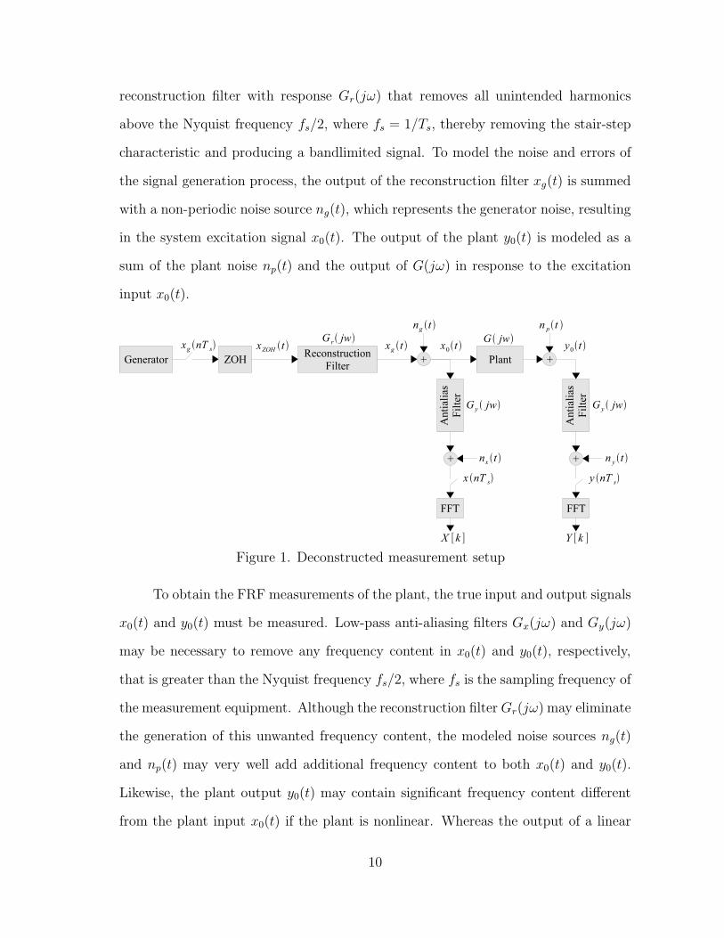
reconstruction filter with response Gr(jω) that removes all unintended harmonics
above the Nyquist frequency fs/2, where fs = 1/Ts, thereby removing the stair-step
characteristic and producing a bandlimited signal. To model the noise and errors of
the signal generation process, the output of the reconstruction filter xg(t) is summed
with a non-periodic noise source ng(t), which represents the generator noise, resulting
in the system excitation signal x0(t). The output of the plant y0(t) is modeled as a
sum of the plant noise np(t) and the output of G(jω) in response to the excitation
input x0(t).
Figure 1. Deconstructed measurement setup
To obtain the FRF measurements of the plant, the true input and output signals
x0(t) and y0(t) must be measured. Low-pass anti-aliasing filters Gx(jω) and Gy(jω)
may be necessary to remove any frequency content in x0(t) and y0(t), respectively,
that is greater than the Nyquist frequency fs/2, where fs is the sampling frequency of
the measurement equipment. Although the reconstruction filter Gr(jω) may eliminate
the generation of this unwanted frequency content, the modeled noise sources ng(t)
and np(t) may very well add additional frequency content to both x0(t) and y0(t).
Likewise, the plant output y0(t) may contain significant frequency content different
from the plant input x0(t) if the plant is nonlinear. Whereas the output of a linear
10

plant contains only the same frequency components as the input, it is possible for the
output of a nonlinear plant to contain frequency content at higher frequencies than
the input.
Following the anti-aliasing filters, the input and output signals are corrupted
with additive noise sources nx(t) and ny(t), respectively, to represent the measurement
noise before being sampled to obtain x(t) and y(t), respectively. Mathematically, the
sampled measurements can be represented as
x(t) = (x0(t) + nx(t))∞∑
n=−∞
δ(t− nTs). (3)
In practice, these time-sampled measurements could represent the output of an
analog-to-digital converter (ADC).
The sampled continuous-time measured signals x(t) and y(t) are transformed
to the frequency domain using the discrete Fourier transform (DFT) to obtain X [k]
and Y [k], respectively. This DFT consists of the the analysis equation
X [k] =
N−1∑
n=0
x[n]e−j2πnk/N (4)
and the synthesis equation
x[n] =1
N
N−1∑
k=0
X [k]ej2πnk/N , (5)
where x[n] is the discrete-time representation of the sampled continuous-time signal
x(nTs).
In frequency-domain system identification, the FRF estimate G(jω) of the true
plant transfer function G0(jωk) consists of transfer function measurements G(jωk) at
11

discrete frequencies ωk, where
G(jωk) =Y [k]
X [k](6)
and
ωk =2πk
NTs(7)
with uniform sampling period Ts and N number of samples. Because x[n] has finite
length and X [k] specifies the frequency of x[n] at only a finite set of frequencies, it
is possible to observe both the smearing and leakage of frequency content in X [k].
To prevent this, an integer number of periods must by measured, and all frequency
content in x[n] must reside at the sampled frequencies ωk of the DFT.
Assuming the excitation waveform is periodic with sample length N and
measurements are collected for M number of periods, as shown in Fig. 2, the m-
th estimate of G(jω) is
Gm(jωk) =Ym[k]
Xm[k], (8)
where Xm[k] and Ym[k] are the N -length DFT of the m-th period of the measured
waveforms x[n] and y[n], respectively.
Several methods exist for finding an average FRF estimate GM(jωk) of the M
number of G(jωk) estimates. One approach is to average the M number of input and
output measurement periods before calculating the FRF estimate as
GM(jωk) =
∑Mm=1 Ym[k]
∑Mm=1Xm[k]
. (9)
Assuming that the measured Fourier coefficients can be represented as
Xm[k] = X0[k] +NXm[k] (10)
Ym[k] = Y0[k] +NYm[k], (11)
12

G1(jωk) Gm(jωk) GM(jωk)
m = 1 m m = M
x(t)y(t)x[n]
y[n]
1 N 1 N 1 Nn
Figure 2. m-th FRF estimate
where NXm[k] and NYm
[k] are the noise contributions from nx(t) and ny(t) in the
m-th estimate, and NX [k] and NY [k] are circular-complex normally distributed [41]
such that
E{NX [k]} = limM→∞
1
M
M∑
m=1
NXm[k] = 0 (12)
E{NY [k]} = limM→∞
1
M
M∑
m=1
NYm[k] = 0, (13)
then it can be shown that
limM→∞
GM(jωk) =Y0[k]
X0[k]= G0(jωk). (14)
Thus, as the number of estimates M approaches infinity, the bias error of the average
FRF estimate GM(jωk) calculated using Eq. (9) approaches zero.
13

The primary goal in the design of excitation signals is to maximize the quality of
the average FRF estimate GM(jωk) for a given measurement time and peak amplitude
of excitation. The quality of the result can be established by analyzing the variance
of G(jωk) which is estimated as
σ2M (jωk) =
1
M(M − 1)
M∑
m=1
∣
∣
∣Gm(jωk)− GM(jωk)
∣
∣
∣
2
, (15)
where the plant transfer function is estimated as
GM(jωk) =1
M
M∑
m=1
Gm(jωk) ≈ G0(jωk). (16)
As σ2M(jωk) decreases for a given frequency point wk, the quality of GM(jωk) at wk
improves. However, this does not necessarily imply that GM(jωk) is a good estimate
of G0(jωk), since σ2M(jωk) does not account for any bias error in GM(jωk). Rather,
σ2M(jωk) describes a confidence ball
∣
∣G0(jωk)− GM(jωk)∣
∣ < ασM(jωk)) (17)
in the complex plane for GM(jωk), where α is chosen to achieve the desired level of
confidence.
Generally speaking, minimizing the sources of measurement error will help to
reduce the number of samples M required to achieve a quality FRF estimate with
a specified confidence level. Extensive research has been performed with the goal of
reducing the error in FRF measurements caused by influences such as noise, nonlinear
distortions, and non-ideal test hardware [?, 28, 42]. One particular area of focus
is on the design of excitation signals. Through the careful selection of excitation
14

signal parameters, many distortions that commonly plague FRF measurements can
be reduced or even eliminated.
2.3. Multisine Excitation Signals
Advances in DSP techniques and hardware, especially the implementation of the
fast Fourier transform (FFT) [43] for efficient calculation of the the DFT, enable the
use of multisine excitation waveforms rather than single sinusoids for obtaining FRF
measurements. The primary benefit is that multisine input signals enable the system
response to be measured at multiple discrete frequencies of interest simultaneously
rather than consecutively. As will be shown, this can dramatically reduce the
required measurement time needed to obtain an acceptable FRF variance compared
to consecutive single sine measurements.
In general, a multisine signal consists of a sum of two or more harmonically
related sinusoids with programmable amplitudes, phases, and frequencies [44]. It is
mathematically defined as
x(t) =F∑
k=1
Ak sin (2πfkt + φk), (18)
where Ak, fk, and φk are elements of amplitude, frequency, and phase vectors,
respectively, and F is the number of harmonics in the signal. In contrast, a single or
stepped sine is a pure sine wave defined as
x(t) = A sin (2πft+ φ), (19)
where the frequency is updated for every measurement.
Much research has been devoted to the minimization of the crest factor (Cr) of
multisine signals [45–48]. This parameter is useful for characterizing excitation signals
as it quantifies the ratio of the peak amplitude of a signal to the power of the signal.
15

This factor is relevant when one considers that a high power input signal is beneficial
as it increases the signal-to-noise ratio (SNR) of the experiment, thus leading to a
reduction in σ2M (jωk). However, a signal with sufficiently small peak amplitude is
necessary for the plant to approximate a linear system and to prevent saturation of
the measurement system. Therefore, an excitation signal with minimum crest factor
is preferred. Assuming all of the signal power is constrained to the frequency range
of interest, the crest factor of a periodic signal x(t) is
Cr(x) =max
t{|x(t)|}
√
1T
∫
T|x(t)|2 dt
=xmax
xrms, (20)
where T is the period of x(t). For example, a single sinusoid with a peak amplitude of
1 has an rms value of 1/√2 and a crest factor of
√2 ≈ 1.414, whereas a square wave
with a peak amplitude of 1 has an rms value of 1 and a crest factor of 1. It is easy to
see that for a given peak amplitude, a square wave excitation signal has a lower crest
factor than a single sinusoid and is capable of perturbing a system with more power.
This becomes even more apparent when considering the Fourier series of a square
wave, which consists of a fundamental sinusoid with a peak amplitude of 4/π and
a infinite number of harmonically-related sinusoids with decreasing amplitude over
frequency. Actually, a square wave is a special case of a non-bandlimited multisine
signal.
Another important parameter to consider when comparing excitation signals
is the signal time factor (Tf) [44]. The time factor of the input signal x(t) defines
the minimum measurement time required for all excitation frequencies ωk in x(t) to
obtain FRF measurements with a minimum relative accuracy. In a multisine signal,
this is limited by the test frequency with the minimum SNR. The time factor is
16

calculated [41] as
Tf(x) = maxk
{
0.5Cr2(x)X2
rms
|X [k]|2}
, (21)
where
X2rms =
N∑
k=1
|X [k]|2N
(22)
and x[n] is periodic with sample length N . Eq. (21) has been normalized by
introducing the scale factor 0.5 such that a pure sinusoid has a time factor of 1.
When considering the transient response of the plant and measurement system
when initially applying an excitation signal, the difference in total measurement time
for single sine and multisine signals with the same time factor becomes apparent.
Each time a new input signal is applied, it is necessary to wait for a time Tw until the
transient response of the system decays to an acceptable level. Assuming a very high
SNR and frequency dependent waiting time Tw(f), the minimum total measurement
time when using a stepped sine excitation signal to test F number of fk frequencies
is
Tss =
F∑
k=1
{1/fk + Tw(fk)}. (23)
Under the same conditions, the total measurement time for a multisine signal is
Tms = 1/f0 +maxfk
{Tw(fk)}, (24)
where 1/f0 is the period of the multisine signal. Whereas the stepped sine signal
incurs a waiting time penalty at each step in frequency, a system excited with a
multisine signal only needs time for the transient to settle once, and that time is set
by the test frequency with the longest settling time. This shows quite obviously that
under conditions of high SNR, a multisine excitation will outperform a stepped sine
excitation in regards to total test time. On the other hand, if the SNR is very low,
17

the waiting time Tw becomes small in comparison to the measurement time required
to obtain an FRF measurement with acceptable accuracy. Assuming the power in
the multisine is equally distributed across F frequencies and the measurement noise
is flat across the frequency range of interest, the multisine excitation must be applied
F times longer than each single sine excitation. Therefore, in a measurement system
with low SNR, the total measurement time for multisine and stepped sine excitations
are approximately equal [17].
In general, the ease at which multisine signals can be generated with today’s
DSP techniques and the resulting decrease in total measurement time has made
multisine excitation signals for system identification in the frequency-domain the
preferred choice. Not surprisingly, several variations of multisine signals have been
developed over the years, each with their own advantages and disadvantages. In the
next several sections, the major classes of multisine signals are reviewed.
2.3.1. Schroeder Multisine
In 1970, Schroeder published a method [49] for reducing the crest factor
of multisine signals with flat amplitude spectra and uniformly spaced frequency
components by choosing the phases φk of Eq. (45) such that φk = −k(k − 1)π/K.
This solution does not necessarily find the minimum crest factor, but its closed form
nature usually enables the crest factor of a multisine signal to be reduced with little
computational complexity. The typical crest factor of a Schroeder multisine with flat
amplitude spectra and uniformly spaced frequency components is approximately 1.6-
1.7. In practice, it is also common to use the Schroeder phases for multisine signals
without flat amplitude spectra or uniformly spaced frequency components. However,
applying the Schroeder phases to a signal with a pseudo-log spaced frequency spectra
results in a crest factor of around 3 or higher [44]. In this case, it is advantageous to
18

use another form of crest factor minimization such as a random phase distribution or
an iterative crest factor optimization algorithm.
2.3.2. Multisines for Nonlinear Detection
All practical systems are nonlinear in nature. For discussion purposes, Evans
assumes the plant G(jω) can be reduced to a linear system in parallel with a static
nonlinear system as shown in Fig. 3 [27]. Typically, it is assumed that the nonlinear
output contribution yNL(t) is dominated by the linear output contribution yL(t) for a
sufficiently small peak value xmax of x(t). This is a perfect example of why minimizing
the crest factor of x(t) is so important for the accurate estimation of G(jω) in an
acceptably short measurement time. However, it is not always obvious what is an
acceptable value of xmax and what effect the nonlinear contributions yNL(t) have on
the measured output y(t), where y(t) = yL(t) + yNL(t). Particular attention must be
paid during testing to ensure that any effect of nonlinear contributions is reduced.
Linear
Nonlinear
x(t) y(t)
yNL(t)
yL(t)
Figure 3. Parallel nonlinear model structure
Assuming stochastic errors are small and neglected, Evans shows that the FRF
estimate G(jωk) at the excitation frequencies wk is
G(jωk) = Y (jωk)/X(jωk) =YL(jωk)
X(jωk)+
YNL(jωk)
X(jωk)(25)
From this it can be seen that any non-zero terms of YNL(jωk) will result in a systematic
bias and/or scatter of the FRF estimate. Assuming that the the nonlinear system
19

can be represented, rather simply, by the power-series
yNL(t) =P∑
p=1
γpxp(t), (26)
where P is the maximum order of the nonlinear system, the output contribution
YNLp(jω) of the p-th order term of the system nonlinearity can be found using
convolution in the frequency-domain. For example, the output of a quadratic
nonlinearity is
YNL2(jω) = γ2 [X(jω) ∗X(jω)] , (27)
and the output of a cubic nonlinearity is
YNL3(jω) = γ3 [X(jω) ∗X(jω) ∗X(jω)] . (28)
If X(jω) is non-zero for a discrete set of frequencies wk, then YNLp(jω) is non-zero
for all combinations of p number of frequencies from wk. In the case of a multisine
signal as defined in Eq. (45), the frequencies of nonlinear contributions are located at
fi± fj and fi± fj ± fk for quadratic and cubic nonlinear systems, respectively, where
i = 1, 2, . . . , F , j = 1, 2, . . . , F , and k = 1, 2, . . . , F .
To help understand the effects of the nonlinearities, Evans divides the
contributions into two categories, Type I contributions and Type II contributions
[27]. Type I contributions are located at the test frequencies fk or at DC and are
generated by combinations of equal positive and negative frequencies. For a quadratic
nonlinearity, a combination of fk − fk results in a contribution at DC. Likewise, a
combination of fi − fi + fk for a cubic nonlinearity results in a contribution at fk.
Type I contributions have the same phase as the original test frequency, and as such,
will introduce a systematic bias into the FRF estimate. The total number of Type I
20

contributions depends only on the order of the nonlinearity. The distribution of fk
has no effect.
Type II contributions include all other frequency combinations. This includes
the quadratic nonlinearity combinations fi ± fj 6= 0 and the remaining cubic
nonlinearity combinations fi ± fj ± fk. Unlike Type I contributions, the phases of
Type II contributions depends on the phases φk of the multisine input and the order
of the nonlinearity. Therefore, Type II contributions introduce a varying bias in the
form of scatter.
Several types of multisine excitation signals have been developed to reduce
nonlinear distortions in y(t) contributed by yNL(t) and to aid in the detection
of nonlinear contributions. Odd, odd-odd, and no-interharmonic-distortion (NID)
multisines are reviewed in the following sections.
2.3.2.1. Odd Multisine
An odd multisine excitation signal contains signal power at only the odd
harmonics of the fundamental frequency component f0 by restricting the frequency
vector fk of Eq. (45) to fk = (2k−1)f0. The primary benefit of only exciting the odd
harmonics is that all Type I and Type II even-order nonlinearity contributions will
fall at either DC or the unexcited even harmonics. Therefore, the linear contribution
of the output YL(jωk) and all even-order nonlinearity contributions are orthogonal
in the frequency domain [20]. Not only does this prevent the output Y (jωk) from
being distorted by the even-order nonlinearity contributions, but it also enables the
even-order nonlinearity contributions to be detected by analyzing the unexcited even
harmonics at the output. However, the output Y (jωk) still includes both Type I and
II odd-order nonlinearity contributions. The Type I odd-order contributions always
fall on the test frequencies, and the Type II odd-order contributions consist of an
21

odd sum of odd harmonics, which may result in contributions at the excited odd
harmonics.
2.3.2.2. Odd-Odd Multisine
The odd-odd multisine is similar to the odd multisine, except that only every
other odd harmonic is excited according to fk = (4k − 3)f0. At the (4k − 3)f0
frequencies, the output consists of the linear contribution YL(jωk), all of the Type I
odd-order nonlinearity contributions, and some of the Type II odd-order nonlinearity
contributions. At the (4k − 1)f0 frequencies, the output includes only some of the
Type II odd-order nonlinearity contributions. The output includes only Type II
even-order nonlinearity contributions at the (4k − 2)f0 and (4k)f0 frequencies, and
all Type I even order nonlinearities again fall at DC [41]. Therefore, both the even-
order and odd-order nonlinearity contributions can be detected and characterized by
analyzing the unexcited even and odd harmonics at the output. Despite the added
advantages over the odd multisine, the output Y (jωk) still suffers from Type II odd-
order nonlinearity distortions. In addition, the odd-odd multisine suffers from reduced
frequency resolution compared to the odd multisine.
2.3.2.3. NID Multisine
A no-interharmonic-distortion (NID) multisine follows the form of Eq. (45), but
the frequency vector fk consists of a sub-set of the odd harmonics of f0 such that
all Type II nonlinearity contributions, including odd-order nonlinearities, up to a
certain order are eliminated from the output Y (jωk). Once again, the excitation
signal is restricted to only odd harmonics to prevent any even-order nonlinearity
distortions at the output. However, Type I odd-order nonlinearity distortions still
exist in the output Y (jωk) since these contributions fall at the test frequencies.
Because all significant Type II nonlinearity contributions can be removed, the
FRF measurements exhibit only a systematic bias caused by the Type I odd-order
22

nonlinearity contributions [27]. An example harmonic vector for a multisine signal
with NID properties up to and including fourth order nonlinearities [20] is
fk = f0× [1 5 12 29 49 81 119 141 . . .
207 263 359 459 543 729 775 909 . . .
1097 1213 1405 1649 1853 2077 2461 2653 . . .
3047 3111 3151 3631 4177 4431 5195 5591 . . .
6793 6943 7745 8457 8759 10033 10209 11391 . . .
11783 13281].
(29)
The frequency distribution of an NID multisine tends to be closer to a logarithmic
spacing rather than a linear spacing, as seen in Fig. 4.
100 102 104
1
Harmonics
Amplitude
Figure 4. Frequency distribution of NID multisine
2.3.3. Pseudo Log-Spaced Multisine
A pseudo-log spaced multisine is an approximation of a logarithmic spaced
frequency distribution where each excited frequency component is rounded to the
nearest discrete frequency fk that is a harmonic of the fundamental f0. The harmonic
requirement is imposed such that all frequency components of the multisine signal will
have an integer number of periods for each period of excitation, which is necessary
to prevent leakage errors in the subsequent DFT calculations. An example of a
pseudo-log spaced multisine that excites the frequency band of 1Hz to 100Hz with 12
23

lines per decade and a period of 6 seconds is shown in Fig. 5. The frequency error
between the pseudo log-spacing and the ideal log spacing is shown in Fig. 6. The
design criteria for this particular signal were chosen such that the resulting pseudo
log-spaced frequency distribution has no degenerate frequencies, where degenerate
frequencies refer to adjacent log spaced frequency components that are rounded to
the same pseudo-log spaced frequency. Furthermore, the second harmonic of each
excited frequency falls at an unexcited frequency, thus reducing the effects of nonlinear
contributions in the output measurements [50].
0
0.5
100 101 102
1
Frequency [Hz]
Amplitude
Figure 5. Pseudo log-spaced multisine
Compared to a linear spaced frequency distribution, a logarithmic spacing is
useful for covering a large frequency range with a sparse excitation spectrum. By
reducing the number of frequencies F , more power can be applied at each test
frequency while still limiting the peak amplitude of excitation xmax to the linear
range of the plant. This increases the SNR of the measurements and decreases the
total measurement time needed to achieve a given FRF variance σ2G[k]. Because many
plant models are plotted using log-log scaling, a logarithmic frequency distribution
more accurately measures the plant, whereas a linear frequency spacing would tend
to concentrate measurements at the the higher test frequencies [51].
24

100 101 1020
0.5
1
1.5
2
2.5
3
3.5
4
Frequency [Hz]
Frequency
Error
[%]
Figure 6. Frequency error of pseudo log-spaced multisine
2.4. Signal Sampling
The concept of sampling a continuous time signal is reviewed along with the
conditions necessary to reconstruct the signal exactly from its samples. In addition,
aliasing and undersampling are presented.
2.4.1. The Sampling Theorem
A sampled continuous time signal xp(t) can be represented as the multiplication
of x(t) with a periodic pulse train p(t), where
p(t) =
+∞∑
n=−∞
δ(t− nTs), (30)
resulting in
xp(t) = x(t)
+∞∑
n=−∞
δ(t− nTs). (31)
This is illustrated in Fig. 7. The sampling theorem, proved by Shannon in 1949 [52],
25

x(t)
n− 1 n n+ 1 n+ 2 n+ 3 n+ 4
p(t)
xp(nTs)
Ts
t
1
Figure 7. Impulse train sampling
states that any continuous-time low-pass function x(t) with X(jω) = 0 for |ω| ≥ W
can be exactly determined by its samples at xp(nTs), for integer values of n, if
ωs ≥ 2W, (32)
where ωs = 2π/Ts. Assuming x(t) is sampled at the minimum sampling rate ωs = 2W ,
also known as the Nyquist rate, the original signal can be approximately reconstructed
as x(t) from the samples xp(nTs) according to
x(t) =+N∑
n=−N
xp(nTs)sin (π(2Wt− n))
π(2Wt− n). (33)
26

As the number of samples approaches infinity, the quality of the x(t) estimate
improves, such that
limN→∞
∫ +∞
−∞
|x(t)− x(t)|2 dt = 0. (34)
The need for an infinite number of samples to exactly reproduce x(t) is rather evident
since the domain of a signal cannot be finite in both time and frequency. However,
considering that in practice all time domain signals have inherently finite duration,
the frequency spectrum X(jω) must be nonzero at |ω| ≥ W . If X(jω) is limited to
very small values for |ω| ≥ W , then the reconstructed signal x(t) will contain little
energy outside the support of x(t).
2.4.2. Aliasing
The appearance of signal content at a frequency lower than the true signal
frequency is known as aliasing. For example, the Fourier transform of the sampled
signal xp(t) = x(nTs) is
Xp(jω) =1
Ts
∞∑
k=−∞
X(j(ω − kωs)), (35)
where X(jω) is the Fourier transform of the original continuous-time signal x(t).
Therefore, Xp(jω) is a periodic function consisting of multiple shifted copies ofX(jω).
Given an original bandlimited signal with X(jω) = 0 for |ω| ≥ W , as shown in Fig. 8,
if ws ≥ 2W , then the replicas of X(jω) appearing in Xp(jω) do not overlap. This is
illustrated in Fig. 9. Thus, X(jω) can be recovered exactly from xp(nTs), as stated
by the sampling theorem. However, if ws < 2W , as shown in Fig. 10, then the copies
of X(jω) in Xp(jω) may overlap, and the original X(jw) may no longer be recovered.
2.4.3. Undersampling
The sampling theorem can be further extended by realizing that x(t) does not
need to be limited to the class of low-pass functions. Consider a complex bandpass
27

|X(jω)|
−W W0ω
1
Figure 8. Spectrum of original signal
|Xp(jω)|
−W W0ω
1
ωs 2ωs−ωs−2ωs
Figure 9. Spectrum of sampled signal with ωs > 2W
|Xp(jω)|
0ω
1
ωs 2ωs 3ωs 4ωs−ωs−2ωs−3ωs−4ωs
Figure 10. Spectrum of sampled signal with ωs < 2W
function XBP(jω) that is zero outside the range of Wa < ω < Wb. This can be
represented mathematically as the convolution of a low-pass function XLP(jω) with
a frequency shifted delta function by
XBP(jω) = XLP(jω) ∗ δ(ω − (Wa +W )), (36)
28

where W = (Wb −Wa)/2. Since XLP(jω) = 0 for |ω| ≥ W , then as long as xLP(t) is
sampled at ws ≥ 2W , xLP(t) can be exactly reconstructed as xLP(t) from the samples
according to Eq. (33). Knowing that F−1{δ(ω − (Wa +W ))} = ej(Wa+W )t, then
xBP(t) = ej(Wa−W )txLP(t). (37)
In general, any continuous-time signal with a bandwidth W can be exactly
reconstructed from its samples if ws > 2W .
The process of sampling a signal x(t) at a rate less than 2ωmax, where X(jω) = 0
for |ω| ≥ ωmax is known as undersampling. Because undersampling reduces the rate at
which samples of a signal are collected, it is a useful technique for relaxing the speed
requirements of the digital signal processing system. Plus, as long as the sampling rate
remains greater than twice the bandwidth of the sampled signal and all out-of-band
content is properly rejected, no information from the original signal is lost.
2.5. Undersampled Excitation Signal Design
Undersampling is a proven way to reduce power consumption and computational
complexity in frequency analysis hardware [53]. Since the relationship between the
signal generator and analysis circuitry in the system identification instrumentation
hardware is tightly controlled, frequency aliasing through undersampling can be
implemented in the analysis stage when using properly designed excitation signals [15].
The benefits of undersampling have previously been applied to system identification
in order to reduce the complexity and cost of measurement and processing
equipment. For example, Gamry Instruments, a producer of electrochemical
measurement equipment, designs potentiostats for system identification that use
single sine excitation signals and undersampling techniques for signal measurement
[14]. Specifically, any excitation frequencies greater than 8Hz are undersampled using
the on-board analog to digital converter. When using only single sine excitation
29
signals, it is relatively straight forward to identify prior to sampling if undersampling
should be used. In addition, because the measured signal is dominated by a single
frequency, there is little concern of loss of information due to aliasing.
Using multisine excitation signals in combination with undersampling increases
the complexity of the problem. Without careful selection of the frequencies of
excitation and the undersampling frequency, interference between multiple excited
frequencies can occur in the aliased measurements, thereby resulting in the loss or
corruption of data. One method for undersampling a multisine signal composed of
harmonically related content is to skip one or more periods of the lowest harmonic
component [54]. Specifically, Martnes proposed using this method of undersampling
in performing bio-impedance measurements [16]. Consider a multisine signal that
follows Eq. (45), where f = kf0. If M periods of component f0 are skipped between
samples plus an effective sampling step ∆T , then the period of the undersampling
frequency is found to be
Ts =M
f0+∆T, (38)
where 1/∆T is the Nyquist rate, defined as
1
∆T≥ 2fF . (39)
While this approach to undersampling of multisine excitations signals in system
identification is useful for reducing the speed requirements of the DSP system, it
imposes restrictions on the design of the excitation signal. For example, the frequency
spacing of the excitation signal must be linear, and the lowest frequency component of
the signal must be approximately greater than twice the sampling frequency. These
requirements may make it difficult or impossible to design an optimal excitation
30

signal with respect to test time, test frequencies, noise requirements, and hardware
limitations.
2.6. Typical Methods of Multisine Generation
The development and commercialization of the digital signal processor (DSP)
has eased the difficulty of generating multisine excitation signals. Through the use
of a look-up table (LUT) or recursive algorithm, a DSP can quickly calculate the
digital samples necessary to produce a desired waveform. Using a digital-to-analog
converter (DAC) interfaced to the DSP, these discrete time samples can be readily
converted into a continuous time signal. The hardware requirements of the DAC,
such as the sampling rate, settling time, resolution, and range, are largely dependent
on the parameters of the generated signals.
The digital recursive sinusoidal oscillator is capable of producing a fixed
frequency sinusoidal output. Therefore, a multisine signal generator would require
multiple recursive oscillators, one for each sine component of the multisine output, to
be summed together. On the other hand, a direct digital synthesizer (DDS), which
employs the LUT approach to signal generation, can directly produce either a single
or a multisine excitation. DDS and recursive oscillators are discussed in detail in the
following sections.
2.6.1. Direct Digital Synthesis
Direct digital synthesis (DDS) is a digital technique for creating arbitrary
waveforms synchronized to a fixed frequency reference clock. A simple DDS
architecture is shown in Fig. 11. It consits of an input reference clock fclk, an address
counter, and a programmable-read-only-memory (PROM) LUT. The digital output
of the PROM LUT is interfaced to a DAC in order to convert the digitally produced
waveform into a continuous-time output. In operation, the output of the address
counter is incremented once per cycle of fclk. This output is used as a memory
31

pointer to the PROM LUT, which subsequently outputs the corresponding digital
value stored in said memory location. The PROM LUT is programmed with one
complete cycle of discrete amplitude samples of the desired output waveform. The
address counter is circular, thus, a new cycle of the output signal will commence at
the completion of the previous cycle. For this particular architecture, the period of
the output waveform is often
T =2N
fclk, (40)
and the size of the LUT is 2N ×M bits.
Figure 11. Simple direct digital synthesizer
A more advanced and tunable DDS architecture is shown in Fig. 12. In this
architecture, the circular address counter has been replaced with a phase accumulator.
This performs essentially the same function except that its increment step size can
be adjusted. In addition, the PROM LUT block has been renamed the phase to
amplitude converter to better describe its functionality. However, it still consists of
the same PROM LUT structure as before.
Figure 12. Tunable direct digital synthesizer
The frequency of the DDS output can be adjusted by modifying the frequency
control tuning word that is summed with the feedback from the phase accumulator
32

output. This adjusts the step size of the phase accumulator and changes the number
of fclk cycles that are required to traverse one cycle of the waveform stored in the
phase to amplitude converter block. For phase control of the output signal, a phase
control tuning word is summed with the output of the phase accumulator to control
the phase offset of the output waveform. Lastly, the amplitude of the output waveform
can be adjusted by multiplying the output of the phase to amplitude converter with
an amplitude control tuning word.
Quantization error is introduced at both the output of the phase accumulator
and the output of the phase to amplitude converter. Additional quantization error can
be injected by a bit-wise truncation between the output of the phase accumulator and
the input of the phase to amplitude converter. This truncation is sometimes imposed
to reduce the memory size of the LUT, which can grow prohibitively large otherwise.
Quantization error manifests itself as unwanted spurious spectral components in the
DDS output signal. The difference in output power of the desired signal and the noise
spurs is called spurious free dynamic range (SFDR).
One of the easiest ways to maximize the SFDR of the DDS output, an important
goal of many designs, is to increase the bit-width of the phase to amplitude converter
input. However, as mentioned before, this may lead to an impractically large LUT.
In light of this, a considerable amount of DDS research has been dedicated to the
compression of the waveform stored in the LUT. For example, if the waveform is a
sinusoid, its symmetrical properties can be exploited to gain an LUT compression
ratio of 4:1. By storing only one-quarter of the sinusoid in the LUT, the other three-
quarters of the waveform can be reproduced through the addition of some additional
logic for translating the data points.
33
2.6.2. Digital Recursive Sinusoidal Oscillator
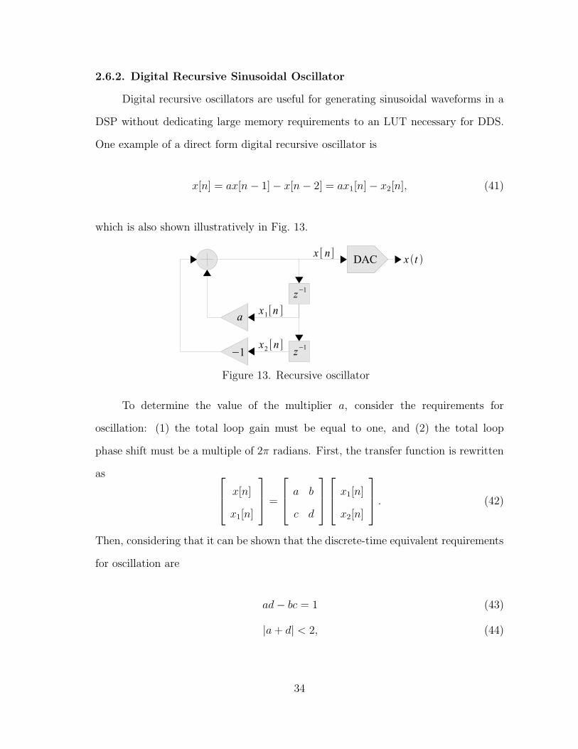
Digital recursive oscillators are useful for generating sinusoidal waveforms in a
DSP without dedicating large memory requirements to an LUT necessary for DDS.
One example of a direct form digital recursive oscillator is
x[n] = ax[n− 1]− x[n− 2] = ax1[n]− x2[n], (41)
which is also shown illustratively in Fig. 13.
Figure 13. Recursive oscillator
To determine the value of the multiplier a, consider the requirements for
oscillation: (1) the total loop gain must be equal to one, and (2) the total loop
phase shift must be a multiple of 2π radians. First, the transfer function is rewritten
as
x[n]
x1[n]
=
a b
c d
x1[n]
x2[n]
. (42)
Then, considering that it can be shown that the discrete-time equivalent requirements
for oscillation are
ad− bc = 1 (43)
|a+ d| < 2, (44)
34

where b = −1, c = 1, and d = 0 in this particular case, it is obvious that there are
many solutions for the value of a. One solution, known as the biquad oscillator, has
a = 2 cos(θ) where θ is the step angle.
Digital recursive oscillators are straight-forward to implement in a DSP because
they are accomplished with only multiplications, additions, and unit delays. However,
these digital operators may be too computationally expensive or power intensive for
an application specific, low-power EIS system. They can also exhibit accumulated
drift errors due to quantization.
35

CHAPTER 3. UNDERSAMPLED SIGNAL
REQUIREMENTS
3.1. Introduction
In this chapter, the generic equation for a multisine excitation signal is defined
along with an explanation of the parameters of most interest to this research. Next,
the assumptions of the measurement system and the system-under-test are declared.
Finally, the requirements for undersampling a multisine excitation signal are outlined
along with an illustrative example.
3.2. Excitation Signal
The focus of this paper is on multisine excitation signals, denoted
x(t) = A0 +M∑
m=1
Am sin(2πfmt+ φm), (45)
where M is the number of tones in the signal, A is a set of amplitudes, φ is a set
of phases, and f defines the frequency distribution of the signal. Elements in f are
defined to be positive and 0 < fm < fm+1 for 1 ≤ m ≤ (M − 1). There is no
upper bound for fM , and no frequencies in f define a DC term. Rather, the DC
term of x(t) is defined by the amplitude A0. All analysis in this paper assumes that
A0 = 0, and the optimization techniques presented here allow for harmonics of the
excitation frequencies to alias to DC. However, it would be straight forward to modify
the presented algorithms to prevent the aliasing of any frequency content to the 0 Hz
DFT bin if it were necessary to prevent the corruption of a DC term in x(t). This
paper uses logarithmic distributions for examples due to their spectral efficiency in
probing over a wide frequency range and applicability to EIS measurement systems.
The design methods presented herein are not dependent on nor specify A or
φ. However, extra consideration given to A and φ may be warranted if nonlinear
36

detection through the measurement of non-excitation frequencies is implemented.
The techniques discussed can result in the aliasing of multiple harmonic frequencies
to the same DFT frequency bin. If the coincident harmonics are out of phase, then
the sampled signal component generated by the system non-linearity is attenuated.
3.3. Measurement Assumptions
A block diagram of the basic impedance spectroscopy test setup is shown in
Fig. 14. The system-under-test is described as an LTI system GL(jω) in parallel with
a nonlinear system GNL(jω) [20]. The impedance spectroscopy hardware generates
an excitation signal x(t) with a digital-to-analog converter (DAC) followed by a
reconstruction filter. Conversely, the instrumentation hardware measures the system
input x(t) and system output y(t) with two analog-to-digital converters (ADC). The
discrete time digital outputs of the ADC circuits are converted to the frequency
domain with DFT processors for further analysis. With this model assumed for the
system-under-test, the system output is
Y (jω) = X(jω)GL(jω) +X(jω)GNL(jω). (46)
It is the X(jω)GNL(jω) term of the system output that can result in harmonic
frequency components. If the magnitudes of these harmonic frequencies are significant
and they fall at excitation frequencies in x(t) after sampling, the ability of the
instrumentation hardware to extract the X(jω)GL(jω) term of Y (jω) is diminished.
3.4. Problem Statement
If the system-under-test combined with the instrumentation equipment
constitutes an LTI system, then the measured system output will contain no harmonic
frequency components other than the fundamental frequencies. The system output
can be undersampled without loss of information as long the excitation frequencies
37

Reconstruction
FilterDAC
GL(jω)
GNL(jω)
AD
C
AD
C
System-Under-Test
x(t) y(t)
DFT DFT
X[k] Y[k]
Impedance
Spectroscopy
Instrumentation
Figure 14. Basic measurement setup.
defined in f remain orthogonal after sampling. This requires that
a(fi) 6= a(fj) for i 6= j (47)
where
a(f) =
∣
∣
∣
∣
f − Fs
⌊
f
Fs
+1
2
⌋∣
∣
∣
∣
(48)
is the absolute value of the frequency alias of f when sampled at Fs. Note that all of
the frequencies in f , including f1, may alias to a lower frequency.
In addition, each excitation frequency must be coincident to a DFT bin center
frequency after sampling to prevent spectral leakage. Since both the magnitude and
phase information of the sampled output signal are required for proper estimation of
the frequency transfer function, the excitation frequencies cannot alias to the 0 Hz
DFT bin. Therefore, the aliases of f must be a subset of d, written
a(f) ⊆ d (49)
38

where
dn = n/T for n = 1, 2, · · · , ⌊(N − 1)/2⌋ (50)
is the set of non-zero positive DFT bin frequencies that compose set d. The excitation
signal period T is related to the output sampling frequency and the total number of
DFT bins by N = FsT . The 0 Hz DFT bin is void of any excitation frequencies after
sampling and is available to hold the alias of one or more harmonic frequencies.
Since the system-under-test G(jω) is nonlinear, f must also be selected such that
the non-fundamental harmonic frequencies in Y (jω) do not alias to the same DFT
frequency as the alias of an excitation frequency. For the purpose of this analysis,
the dominant harmonic frequency components in the system output that are used
for nonlinear detection are defined as the set h. For example, if 2nd and 3rd order
harmonics are to be monitored for nonlinear detection, then h = {2, 3}. Furthermore,
the cardinality of h is denoted as |h| [55]. Therefore, to ensure that harmonic
frequencies in h remain orthogonal to excitation frequencies in f after sampling,
a(fn) 6= a(hifm) (51)
for all 1 ≤ i ≤ |h|, 1 ≤ m ≤ M , and 1 ≤ n ≤ M . Note that the alias of single
harmonic frequency will alias to a single DFT bin. However, the set of all monitored
harmonics of an excitation frequency, {h1fm, h2fm, h3fm, · · · , h|h|fm}, may alias to
up to |h| different DFT bins. In other words, all of the harmonics defined in h for a
given excitation frequency fm may not alias to the same DFT bin.
In order to undersample the system output y(t) without spectral leakage or
distortion from harmonics defined in h, the excitation distribution f must satisfy
Eqs. (47), (49), and (51).
39

3.4.1. Illustrative Example
Given these requirements, it is possible to design a multisine excitation signal
that can be undersampled without loss information. To illustrate this effect, an
approximation of a logarithmically-spaced frequency distribution is shown in Fig. 15.
Assuming the aforemention rules are satisfied, then the distribution of Fig. 15 can be
undersampled to obtain the result shown in Fig. 16. The frequency components are
now out of order as a result of aliasing, as shown by the corresponding color coding.
However, the resulting frequency distribution better utilizes the DFT bins, and the
sampling frequency is dramatically reduced compared to Nyquist.
100 101 102
|X(f)|
Sam
plingRate
f[Hz]
Figure 15. Fourier transform of a multisine excitation
0 4.25 8.5
|X[k]|
Sam
plingRate
HalfSam
plingRate
f[Hz]
Figure 16. DFT of multisine excitation after undersampling
40

CHAPTER 4. IMPROVING DFT BIN UTILIZATION
4.1. Introduction
For a given number of tones, M, the only way to increase the DFT bin utilization
is to decrease the total number of DFT bins, N. In this chapter, the MinN -Freef
algorithm is presented for approximating the minimum value of N for a given M. The
results are compared to an exhaustive search for the minimum value of N for small
values of M. Next, the MinN -Targetp algorithm is presented as an extension to the
MinN -Freef algorithm. The MinN -Targetp algorithm generates a mutisine excitation
signal that approximates a desired frequency distribution, all while attempting to
maximize the DFT bin utilization. Finally, a numerical example is provided to
demonstrate the MinN -Targetp algorithm.
4.2. MinN-Freef Algorithm
Of particular interest is the minimum value of N , Nmin, for which a solution
exists for f since this maximizes the DFT bin utilization. However, there are an
infinite number of unique frequency distributions that alias to the DFT frequencies
defined in d, thus resulting in an infinite number of solutions that must be evaluated
while searching for Nmin.
In order to bound the optimization problem, it is necessary to define a finite set
of frequency distributions to evaluate that includes the solution to f that minimizes
N . This can be achieved by limiting f to be a subset of d, written f ⊆ d. Eqs. (47)
and (49) allow the search space to be bounded to f ⊆ d since they only operate on
a(fm) and a(f), which, by definition, are subsets of d. Likewise, it can be seen that
Eq. (51) also operates on a(fm) when written in the form
a(fn) 6= a(hia(fm)). (52)
41

The substitution of
a(hifm) = a(hia(fm)) (53)
into Eq. (52) can be proved valid by expanding Eq. (52) to
hifm − Fs
⌊
hifmFs
+1
2
⌋
= hi
(
fm − Fs
⌊
fmFs
+1
2
⌋)
− Fs
hi
(
fm − Fs
⌊
fmFs
+ 12
⌋)
Fs+
1
2
(54)
using the more general definition for frequency aliasing of
a(f) = f − Fs
⌊
f
Fs+
1
2
⌋
. (55)
Distributing hi, subtracting hifm, and dividing by −Fs leaves
⌊
hifmFs
+1
2
⌋
= hi
⌊
fmFs
+1
2
⌋
+
⌊
hifmFs
− hi
⌊
fmFs
+1
2
⌋
+1
2
⌋
. (56)
The property ⌊x+ k⌋ = ⌊x⌋+k, where x ∈ R and k ∈ Z, can be applied by recognizing
that
hi
⌊
fmFs
+1
2
⌋
∈ Z (57)
since hi represents a harmonic multiplier and, by definition, must be an integer. Thus,
Eq. (56) reduces to
⌊
hifmFs
+1
2
⌋
=
⌊
hi
⌊
fmFs
+1
2
⌋
+hifmFs
− hi
⌊
fmFs
+1
2
⌋
+1
2
⌋
. (58)
Finally, canceling of terms leaves
⌊
hifmFs
+1
2
⌋
=
⌊
hifmFs
+1
2
⌋
. (59)
42

In the end, the solution space for f can be limited to(
|d|M
)
possibilities. Also
worth noting is that the specific values for T and Fs can be ignored while optimizing
f to minimize N since T and Fs are constrained by the relationship N = FsT . The
resulting minimum value of N for small values of M found after an exhaustive search
of all(
|d|M
)
possible solutions is plotted in Fig. 17. This shows that Nmin typically
increases when either M or |h| increases, but in some instances, M can be increased
without any change to Nmin.
2 3 4 5 6 7 8 9 105
10
15
20
25
30
35
40
45
50
Nmin
M
h = {2}h = {2, 3}h = {2, 3, 4}
Figure 17. Minimum value of N for which a solution exists for f .
Executing an exhaustive search to find Nmin becomes increasingly difficult for
large values of M . Therefore, presented here is an iterative algorithm, titled the
MinN -Freef algorithm, that operates on the free variable f to find Nmin which
satisfies Eqs. (47), (49), and (51). The algorithm solves for f and Nmin by repeatedly
incrementing N and operating on f until a solution is found to exist. The inputs to
the algorithm are the set of harmonic frequencies h, the number of non-DC tones in
the multisine excitation M , and the required excitation signal period T .
43

It has been shown that the search space for the MinN -Freef algorithm can be
reduced to the finite set of DFT frequencies d without affecting Nmin. However, for
each iteration of the algorithm, the search space can actually be reduced further by
recognizing that some harmonics defined in h may automatically exclude some DFT
frequencies in d from holding an excitation frequency after aliasing. This occurs
when an excitation frequency fm and one of its harmonics hifm alias to the same
DFT frequency dn, thereby resulting in corruption of the original excitation frequency
after sampling. The reduced search space is denoted d′, where the prime (′) indicates
that d′ is a subset of the original set d. Because the search space had already been
reduced from f to d, d′ can be defined as
d′ =
x ∈ d : x /∈|h|⋃
i=1
a(hix)
. (60)
The MinN -Freef algorithm sequentially solves for one frequency fm in f at a
time for a given value of N . Each time a solution for another frequency fm is chosen,
the search space d′ is reduced. This limits the set of possible solutions for other
frequencies in f . There are three reasons for this reduction in d′.
1. One frequency in d′ must be reserved to hold the excitation frequency fm.
2. The harmonics of fm may alias to other DFT frequencies defined in d′. These
DFT frequencies are therefore no longer available to hold the alias of an
excitation frequency. For a potential solution x, the set of relevant DFT
frequencies is
α(x) =
y ∈ d′ : y ∈|h|⋃
i=1
a(hix)
. (61)
3. No harmonics of frequencies in f can alias to the same DFT frequency as the
solution chosen for fm. Thus, any DFT frequency remaining in d′ that has a
44

harmonic defined in h that aliases to the same DFT frequency containing fm
is not a valid solution for other frequencies in f . For a potential solution x, the
set of relevant DFT frequencies is
β(x) =
y ∈ d′ : x ∈|h|⋃
i=1
a(hiy)
. (62)
For example, if d = {1, 2, 3, 4}, h = {2}, T = 1, and N = 9, then d′ = {1, 2, 4} since
the 2nd harmonic of d3 aliases to d3. Likewise, α(d′3) = d′1 since the 2nd harmonic of
d′3 aliases to d′1, and β(d′3) = d′2 since the 2nd harmonic of d′2 aliases to d′3.
The objective of the MinN -Freef algorithm is to choose the solution for fm that
minimizes the reduction to d′. This ensures that the maximum number of possible
solutions are available for the next frequency in f to be solved. This objective can be
written as
fm = argminx∈d′
|x ∪α(x) ∪ β(x)| . (63)
Once fm is chosen for a given d′ and h, the set of DFT frequencies available for the
next solution frequency becomes
d′′ = d′ \ fm \α(fm) \ β(fm), (64)
where \ is the notation for set subtraction. Eq. (64) ensures that all future solution
frequencies found for f will reside in empty DFT bins, and the associated harmonics
in h will not distort any previous solution frequencies already found for f .
The complete sequence of steps that compose the MinN -Freef algorithm are
outlined here. The pseudo-code shows that the algorithm increments N until a valid
solution for f that satisfies Eqs. (47), (49), and (51) is found. The value of N at
completion of the algorithm is Nmin.
45

1. Begin withN = 2M+1. This is the minimum possible value forN if h = ∅. Two
DFT bins are required to hold the positive and negative frequency components
of each of the M tones in x(t), and the 0 Hz DFT bin must remain empty.
2. Find the set of non-zero positive DFT frequencies d′ per Eq. (60) that are not
corrupted by the aliases of their own harmonics defined in h.
3. Start with m = 1.
4. Solve for fm using Eq. (63).
5. Increment m. If m = M + 1, then the algorithm is complete and Nmin = N .
6. Use Eq. (64) to remove all DFT frequencies from d′ that are not eligible for
future solutions to frequencies in f . If d′′ = ∅, then a solution to f does not
exist for the current value of N . Increment N and go back to step 2.
7. Substitute d′′ for d′ and return to step 4.
The value of Nmin found with the MinN -Freef algorithm is plotted in Fig. 18
across a range of tones from 2 ≤ M ≤ 50 and for three different sets of harmonics.
The algorithm results are identical to the exhaustive search results shown in Fig. 17
for 2 ≤ M ≤ 10. As would be expected, increasing the number of harmonics in h also
increases the value of Nmin. This is because the algorithm must accommodate more
harmonic frequencies when mapping harmonic frequencies to DFT frequencies that
are orthogonal to the excitation frequencies. In addition, Nmin typically increases as
M increases. However, note that Nmin can remain constant for consecutive values
of M in some instances. This suggests that it may also be possible in some cases
to increase the DFT bin utilization by increasing M while keeping N constant. To
further explore this point, the MinN -Freef algorithm results are post processed to
reveal the maximum number of tones Mmax for a given value of N for which the
46
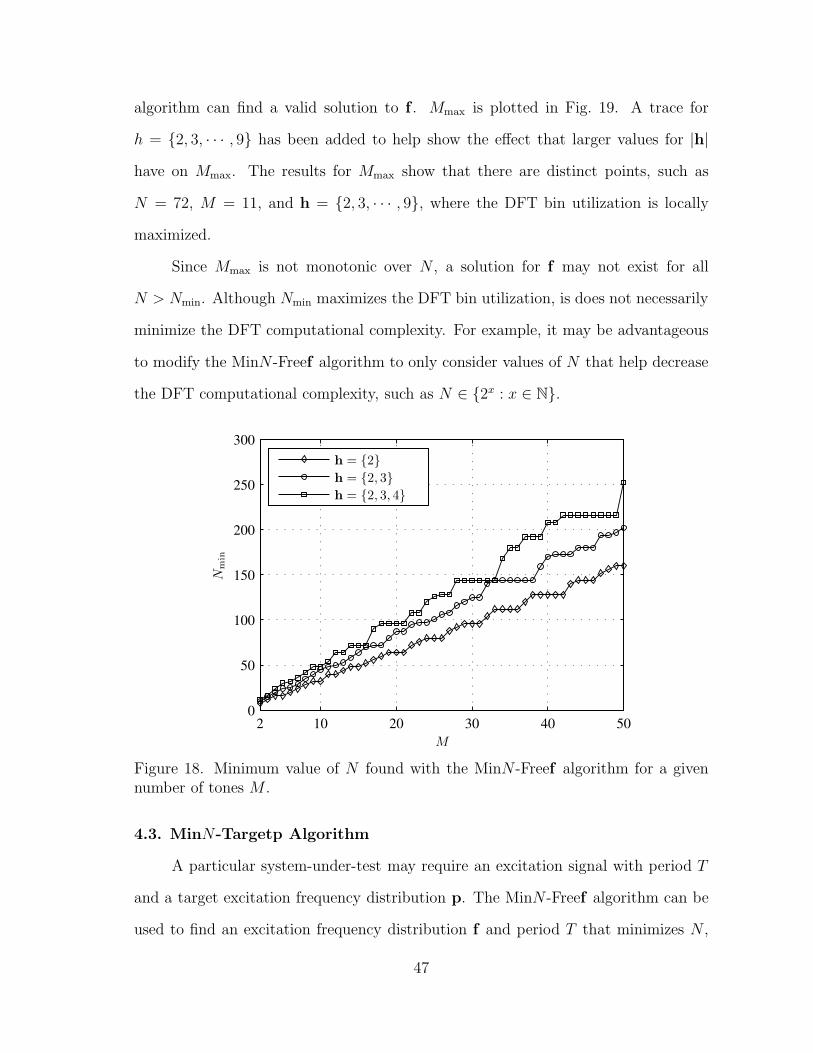
algorithm can find a valid solution to f . Mmax is plotted in Fig. 19. A trace for
h = {2, 3, · · · , 9} has been added to help show the effect that larger values for |h|
have on Mmax. The results for Mmax show that there are distinct points, such as
N = 72, M = 11, and h = {2, 3, · · · , 9}, where the DFT bin utilization is locally
maximized.
Since Mmax is not monotonic over N , a solution for f may not exist for all
N > Nmin. Although Nmin maximizes the DFT bin utilization, is does not necessarily
minimize the DFT computational complexity. For example, it may be advantageous
to modify the MinN -Freef algorithm to only consider values of N that help decrease
the DFT computational complexity, such as N ∈ {2x : x ∈ N}.
2 10 20 30 40 500
50
100
150
200
250
300
Nmin
M
h = {2}h = {2, 3}h = {2, 3, 4}
Figure 18. Minimum value of N found with the MinN -Freef algorithm for a givennumber of tones M .
4.3. MinN-Targetp Algorithm
A particular system-under-test may require an excitation signal with period T
and a target excitation frequency distribution p. The MinN -Freef algorithm can be
used to find an excitation frequency distribution f and period T that minimizes N ,
47
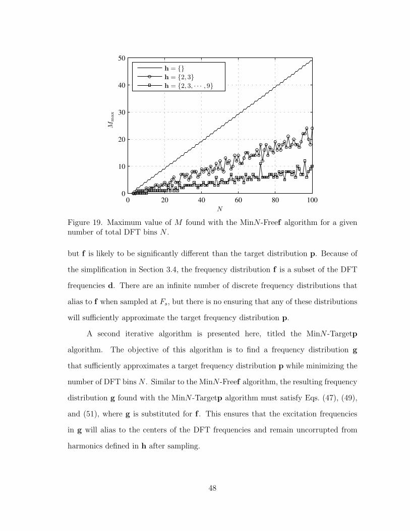
0 20 40 60 80 1000
10
20
30
40
50
Mmax
N
h = {}h = {2, 3}h = {2, 3, · · · , 9}
Figure 19. Maximum value of M found with the MinN -Freef algorithm for a givennumber of total DFT bins N .
but f is likely to be significantly different than the target distribution p. Because of
the simplification in Section 3.4, the frequency distribution f is a subset of the DFT
frequencies d. There are an infinite number of discrete frequency distributions that
alias to f when sampled at Fs, but there is no ensuring that any of these distributions
will sufficiently approximate the target frequency distribution p.
A second iterative algorithm is presented here, titled the MinN -Targetp
algorithm. The objective of this algorithm is to find a frequency distribution g
that sufficiently approximates a target frequency distribution p while minimizing the
number of DFT bins N . Similar to the MinN -Freef algorithm, the resulting frequency
distribution g found with the MinN -Targetp algorithm must satisfy Eqs. (47), (49),
and (51), where g is substituted for f . This ensures that the excitation frequencies
in g will alias to the centers of the DFT frequencies and remain uncorrupted from
harmonics defined in h after sampling.
48

The inputs to the MinN -Targetp algorithm are the set of harmonic frequencies
h, the required excitation signal period T , the target frequency distribution p, and
the maximum error e allowed between frequencies in g and p. The maximum relative
error e can be written as
∣
∣
∣
∣
gm − pmpm
∣
∣
∣
∣
≤ e for 1 ≤ m ≤ M. (65)
Because of the additional input requirements, the distribution g found with the MinN -
Targetp algorithm may not alias to the same set of DFT frequencies as the distribution
f found with the MinN -Freef algorithm.
Like the MinN -Freef algorithm, the MinN -Targetp algorithm repeatedly
increments N until a solution to g is found. For each iteration of the algorithm, the
search space for g is recalculated. Unlike the MinN -Freef algorithm, the search space
for the MinN -Targetp algorithm cannot be reduced to the set of DFT frequencies.
Instead, a distinct search space Sm is defined for each frequency gm in g, resulting in
M search spaces in total. The search space Sm consists of all frequencies that satisfy
the limit defined by e in Eq. (65) and also alias to a DFT frequency. Thus, the search
spaces are defined as
Sm =
{
x ∈ Z :
∣
∣
∣
∣
x− pmpm
∣
∣
∣
∣
≤ e
}
for 1 ≤ m ≤ M (66)
where
Z = {x : a(x) ∈ d′} (67)
is the set of all frequencies that alias to d′ when sampled at Fs. Notice in Eq. (67)
that the set of DFT frequencies d has been reduced to d′ per Eq. (60).
The total number of possible solutions to g is limited to∏M
m=1 |Sm|. However,
recognizing that more than one frequency in Sm may alias to the same DFT
49

frequency allows the total number of possible solution combinations to be reduced to∏M
m=1 |a(Sm)|. If the allowed error e between gm and pm is sufficiently large, then the
maximum number of possible solutions is∏M
m=1 |d′| = |d′|M . Since
(|d|M
)
≤ |d′|M , (68)
adding the additional requirement of Eq. (65) to the existing requirements of
Eqs. (47), (49), and (51) for the MinN -Targetp algorithm can greatly increase the
complexity of the problem.
The MinN -Targetp algorithm is similar in construction to the MinN -Freef
algorithm but adds a means for monitoring which frequencies in g have been solved
and which frequencies remain to be solved. This is tracked with set u, where guiis an
unsolved frequency in g. For example, if solutions for g1, g4, and g5 have been found
and frequencies g2, g3, and g6 have yet to be solved, then u = {2, 3, 6} and |u| = 3.
It is necessary to track the progress of solving g using set u since the objective is for
g to approximate the target distribution p. In contrast, the MinN -Freef algorithm
has no such restriction.
Pseudo-code for the MinN -Targetp algorithm is provided here. The algorithm
uses a search operator that sequentially solves for one frequency gm in g at a time,
where m ∈ u. This search operator differs from the MinN -Freef objective function,
Eq. (63), since it must operate over each search space Sm. Although this algorithm
may operate over a larger total search space compared to the MinN -Freef algorithm,
its progress can be accelerated by starting with the resulting Nmin found with the
MinN -Freef algorithm.
1. Apply the MinN -Freef algorithm from Chapter 4.2 to find an initial value for
N .
50

2. Find the set of non-zero DFT frequencies d′ per Eq. (60) that are not corrupted
by the alias of their own harmonics defined in h.
3. Define u = {1, 2, · · · ,M} so solutions to all M frequencies in f will be found.
4. Apply the search operator to find a solution for one gm in g, where g ∈ u. If
the set of possible solutions Suifor any gui
is empty, then increment N and go
to step 2.
5. Update the set of unsolved frequencies to u′ = u \m. If u′ = ∅, the algorithm
is complete and Nmin = N .
6. Use Eq. (64) to remove all DFT frequencies from d′ that are not eligible for
future solutions to frequencies in g. If d′′ = ∅, increment N and go back to
step 2.
7. Substitute d′′ for d′ and u′ for u and return to step 4.
The objective of the search operator used in the MinN -Targetp algorithm is to
minimize the number of DFT bins by intelligently selecting frequencies from the search
spaces Sm that sufficiently approximate the target distribution p. Three candidate
search operators of increasing complexity are presented in this paper to allow the
relative performance of each to be evaluated.
4.3.1. Search Operators
4.3.1.1. Max|d′| Search Operator
The objective of the Max|d′| search operator is to choose the solution for gm
that minimizes the reduction to d′ and ensures that the maximum number of possible
solutions are available for the next frequency in g to be solved. This operator is similar
to the objective function in the MinN -Freef algorithm, Eq. (63).
Application of the Max|d′| search operator begins by determining which DFT
frequencies in d′ have the potential to hold an excitation frequency after sampling.
51

It is possible that there may be no excitation frequencies that alias to a particular
DFT center frequency and also sufficiently approximate a frequency in p per Eq. (65).
The eligible set of DFT frequencies is equivalent to the alias of all frequencies in the
remaining search spaces. This set is labeled b for reference in this paper and can be
written as
b =
|u|⋃
i=1
a(Sui). (69)
Next, the search operator determines which DFT frequencies in b will minimize
the reduction to d′. This is written as
c = argminx∈b
|x ∪α(x) ∪ β(x)| , (70)
where α(x) and β(x) are found with Eqs. (61) and (62), respectively. Note that it is
sufficient for Eq. (70) to operate over the set of DFT frequencies b since a(gm) ∈ b.
The set c of DFT frequencies is then used to define the set Z′ of all possible solutions
to gm that sufficiently approximate p while also aliasing to a DFT frequency in c.
Set Z′ can be written as
Z′ = {x ∈ Z : a(x) ∈ c} . (71)
Assuming that there are multiple frequencies in Z′ for gm, this paper chooses
the solution for gm that minimizes the error between gm and pm. Thus,
gm = argminx∈Z′
(
miny∈u
∣
∣
∣
∣
x− pypy
∣
∣
∣
∣
)
, (72)
where
m = argminx∈u
∣
∣
∣
∣
gm − pxpx
∣
∣
∣
∣
. (73)
52

4.3.1.2. Max|d′|-MinS Search Operator
The Max|d′|-MinS search operator expands on the previous Max|d′| operator.
This operator considers additional criteria to further optimize g and Nmin at the cost
of extra algorithm complexity. After the set of DFT frequencies c that minimize the
reduction in d′ is found with Eq. (70), the Max|d′|-MinS operator chooses a solution
for gm that aliases to a DFT frequency in c and that also has the smallest search
space. This helps to reduce the likelihood that the MinN -Targetp algorithm will
need to increment N in step 4 when Sui= ∅ for any i in 1 ≤ i ≤ |u|.
Continuing from Eq. (70), the set q of indices to unsolved frequencies in g with
the minimum number of possible solutions, at least one of which aliases to a DFT
frequency in c, is defined as
q = argmini∈k
|Si| , (74)
where
k = {i ∈ u : a(Si) ∩ c 6= ∅} . (75)
From this point it is known that m ∈ q, a(gm) ∈ c, and gm ∈ Z′, where Z′ is still
found with Eq. (71). If this defines more than one frequency in Z′, then the specific
solution for gm is chosen in this paper to minimize the error between gm and pm.
Therefore,
gm = argminx∈Z′
(
miny∈q
∣
∣
∣
∣
x− pypy
∣
∣
∣
∣
)
(76)
where
m = argminx∈q
∣
∣
∣
∣
gm − pxpx
∣
∣
∣
∣
. (77)
4.3.1.3. MinS-Max|d′| Search Operator
As the name implies, the MinS-Max|d′| search operator is similar to the Max|d′|-
MinS search operator except that the order of operation is reversed. This operator
first looks for the frequency gm with the smallest search space and then finds which
53

frequency in this search space will minimize the reduction in d′ for the next frequency
in g to be solved.
First, the search space with the fewest number of frequencies is found. This is
labeled as a set, set q, in case there is more than one search space that is equally
small. Thus,
q = argmini∈u
|Si| , (78)
where Si is found with Eq. (66). Set b is then constructed, where b includes all of
the frequencies in the smallest search space or spaces. This is written as
b =
|q|⋃
i=1
Sqi. (79)
Next, the possible solutions for gm listed in b are analyzed to find the frequencies
that minimize the reduction to d′ for the next solution to g. This results in
c = argminx∈b
|a(x) ∪α(x) ∪ β(x).| (80)
Finally, if c contains multiple solutions to gm, then this paper chooses the frequency
that minimizes the error between gm and pm. Thus,
gm = argminx∈c
(
miny∈q
∣
∣
∣
∣
x− pypy
∣
∣
∣
∣
)
, (81)
where m is found using the same Eq. (77) as in the Max|d′|-MinS search operator.
4.3.2. Numerical Example
Consider the example where p = {10, 20, 50} Hz, h = ∅, e = 0.1, N = 8, and
T = 1 second. Given these conditions, Fs = 8 Hz and d′ = d = {1, 2, 3} Hz. Given
54

these inputs, the set of all frequencies that alias to d′ is
Z = {1, 2, 3, 5, 6, 7, 9,
10, 11, 13, 14, 15, 17, 18,
19, 21, 22, 23, 25, 26, 27,
29, 30, 31, 33, 34, 35, 37,
38, 39, 41, 42, 43, 45, 46,
47, 49, 50, 51, 53, 54, 55} Hz,
(82)
according to Eq. (67). For the sake of this example, the maximum value in Z is
limited to 55. Any value greater than 55 is known not to be a solution to g since
(maxp) e = 55. Using Z, the search spaces S1, S2, and S3 for each respective
frequency in g are defined per Eq. 66.
S1 = {9, 10, 11} Hz (83)
S2 = {18, 19, 20, 21, 22} Hz (84)
S3 = {45, 46, 47, 49, 50, 51, 53, 54, 55} Hz (85)
Assuming the MinS-Max|d′| search operator is selected, then the first frequency
to be solved is g1 since S1 has the fewest number of possible solutions, per Eq. (78).
Following along with Eq. (79), b = {9, 10, 11} since q = {1}. Applying b to Eq. (80)
results in c = {9, 10, 11}. In other words, all of the solutions in S1 will eliminate
the same number of DFT frequencies, one to be exact, from d′ if chosen as the
solution for g1. Finally, the solution to g1 is selected according to Eq. (81), resulting
in gm = g1 = 10 Hz. It is not necessary to compute Eq. (73) to find m. The fact that
there is only a single element in q implies that m = q1 = 1.
55

The first solution, g1 = 10 Hz, aliases to the 2 Hz DFT bin when sampled at 8
Hz. Therefore, d′ is reduced to {1, 3} Hz for future solutions, per Eq. (64). There are
no additional DFT frequencies in d′ that must be removed due to corruption from
harmonic frequencies since this example has assumed h = ∅ for simplicity. Given
this update to d′, the solution sets for the remaining unsolved frequencies g2 and g3
become
S2 = {19, 21} Hz (86)
and
S3 = {45, 47, 49, 51, 53, 55} Hz. (87)
Following the same procedure as before for the MinS-Max|d′| search operator
results in q = {2}, b = {19, 21}, c = {19, 21}, gm = 19, and m = 2. Thus, the next
solution is g2 = 19 Hz. Another equally valid solution if g2 = 21 Hz. The particular
result achieved depends on how Eq. (81) is interpreted for multiple solutions. In
this dissertation, the minimum frequency is chosen by default to minimize power
dissipation.
The second solution, g2 = 19 Hz, aliases to the 3 Hz DFT bin. As before, this
reduces d′ to {1} Hz and S3 to {47, 49, 55} Hz. Applying the MinS-Max|d′| search
operator one last time results in q = {3}, b = {47, 49, 55}, c = {47, 49, 55}, gm = 49,
and m = 3. Thus, the last solution is g3 = 49 Hz and the final complete solution is
g = {10, 19, 49} Hz.
56

CHAPTER 5. APPLICATION TO LOGARITHMIC
DISTRIBUTIONS
5.1. Introduction
This chapter demonstrates the use of the MinN -Targetp algorithm to design
pseudo-logarithmically-spaced frequency distributions g with improved DFT bin
utilization that approximate a target distribution p. In addition, nonlinear detection
through harmonic analysis is accommodated by designing g such that harmonics
defined in set h do not corrupt the excitation frequencies after undersampling.
This analysis assumes that the target excitation signal has an ideal-logarithmically-
spaced excitation frequency distribution p with M tones where 0 < pm < pm+1 for
1 ≤ m ≤ (M − 1).
5.2. Pseudo-Logarithmic Mapping
For a typical Nyquist-sampled system, the ideal target distribution p would be
mapped to a pseudo-logarithmically-spaced distribution p by
pm =⌊Tpm⌉
T(88)
for 1 ≤ m ≤ M , where ⌊x⌉ rounds x to the nearest integer. This ensures that each
excitation frequency is coincident to a DFT frequency to prevent spectral leakage
during analysis. T must be sufficiently large to guarantee that all frequencies in p
are unique. A design guideline that ensures this requirement for any logarithmic
distribution with any number of M frequencies is to ensure that the delta between
linear spaced DFT frequencies is less than the smallest delta between adjacent
frequencies in p, written
1
T< p1(α− 1), (89)
57

where
α =
(
pMp1
)1
M−1
. (90)
An additional constraint when mapping p to a Nyquist-sampled pseudo-
logarithmically-spaced frequency distribution is that the lowest frequency p1 should
not be mapped to p1 = 0 Hz. Otherwise the excitation distribution will contain an
undesirable DC component. This constraint can be written as
1
2T< p1. (91)
Both Eqs. (89) and (91) also apply when undersampling with Fs < 2pM .
However, the presence of any harmonics in an undersampled signal may necessitate a
larger T to ensure adequate DFT bins are available for holding harmonics, especially
if some frequencies in p are less than Fs/2.
The maximum allowed error e between frequencies in g and p must be defined
in order to define the frequency search space for each frequency using Eq. (66). The
allowed error cannot be zero unless a valid result to the MinN -Targetp algorithm is
g = p. In general, the minimum limit to e, labeled emin, is defined by the difference
between the logarithmically-spaced target distribution p and the corresponding
pseudo-logarithmically-spaced frequency distribution p. The minimum error between
frequencies in p and g cannot be less than the maximum error between frequencies
in p and p. For a given value of T , emin can be written as
emin = maxm
∣
∣
∣
∣
p′m − pmpm
∣
∣
∣
∣
. (92)
This does not ensure that a solution to g will exist for e = emin, but it does ensure
that a solution to g will not exist for e < emin.
58
A reasonable upper bound for the maximum error emax for logarithmically-
spaced distributions is
emax =α− 1
α+ 1. (93)
This is the limit at which pm(1 + e) = pm+1(1− e). If e > emax, then the assumption
that gm < gm+1 for 1 ≤ m ≤ (M − 1) is no longer guaranteed to be true. If T is
selected such that emax ≤ emin, then a solution for g at e = emax does not exist. In
this situation, T must be increased in order to decrease emin.
5.3. Examples
The MinN -Targetp algorithm and the three search operators are applied to an
example logarithmically-spaced frequency. The objective is to characterize the ability
of the MinN -Targetp algorithm to maximize the DFT bin utilization by minimizing
the total number of DFT bins. The target frequency distribution p that is used for all
examples is composed of 25 logarithmically-spaced tones spanning two decades from
1 Hz to 100 Hz with a period of T = 6 seconds. This distribution is selected from a
previous study in pseudo-logarithmically-spaced frequency distributions [50].
For the defined distribution p, the frequency error between the Nyquist-
sampled pseudo-logarithmically-spaced distribution found with Eq. (88) and the ideal
logarithmically-spaced distribution is shown in Fig. 20. The maximum error between
p and p is 3.7% and is determined by the frequency p2. Thus, emin = 0.037 per
Eq. (92). Note how the frequency error for higher frequency components of p is
greatly diminished in comparison. This is because the DFT frequencies are linearly-
spaced.
5.3.1. Search Operator Comparison
Now, the MinN -Targetp algorithm is applied to the target distribution p. The
allowed error is set to e = emax = 0.0956 to give the algorithm the most flexibility when
populating g. The algorithm is executed three times using a different search operator
59

100
101
102
0
0.5
1
1.5
2
2.5
3
3.5
4
PercentFrequency
Error
Frequency [Hz]
Figure 20. Frequency error of the Nyquist-sampled pseudo-logarithmically-spacedfrequency distribution p that best approximates an ideal-logarithmically-spacedfrequency distribution p, where p1 = 1, pM = 100, M = 25, and T = 6.
each time to determine the effectiveness of each search operator at reducing the
number of DFT bins. This process is repeated for several different sets of harmonics
to see how the harmonics defined in h affect the result. The algorithm output Nmin
is recorded in Table 1 for these different run combinations. The data show that the
additional operations added to the Max|d′| search operator to create the Max|d′|-
MinS and MinS-Max|d′| search operators result in a further improvement in Nmin
for all tested sets of harmonics. Furthermore, the data show that the MinS-Max|d′|
search operator performs equal to or better than the Max|d′|-MinS search operator
in most of these particular test cases. This suggests that it may be advantageous
to place higher priority on optimizing g based on the search space sizes rather than
optimizing g based on the reduction in DFT frequencies. This helps to ensure that a
solution for a particular frequency is found before the search space for that frequency
is eliminated by other solutions. Note that using the MinS-Max|d′| search operator
does not guarantee that the MinN -Targetp algorithm will find the optimal minimum
60

Table 1. MinN -Targetp algorithm output for M = 25, p1 = 1, pM = 100, T = 6, ande = emax.
Nmin
h Max|d′| Max|d′|-MinS MinS-Max|d′|{2} 112 105 88
{2, 3} 153 108 108
{2, 3, 4} 180 126 126
{2, 3, · · · , 6} 293 240 171
{2, 3, · · · , 9} 510 230 256
number of DFT frequencies needed to define g. However, using the MinS-Max|d′|
search operator may produce better results compared to using one of the other two
search operators.
5.3.2. MinS-Max|d′| Performance
Table 2 provides further analysis of the optimized distribution g and number
of DFT bins Nmin found with the MinN -Targetp algorithm using the MinS-Max|d′|
search operator. The resulting sample frequency is calculated as Fs = Nmin/T =
Nmin/6. The DFT bin utilization is equivalent to 2M/Nmin = 50/Nmin. The
improvement in DFT bin utilization compared to a Nyquist-sampled excitation
signal equals the sample frequency, Fs, divided by the Nyquist-sample frequency,
2pM = 200 Hz, assuming the higher frequency harmonics are removed with an anti-
aliasing filter prior to Nyquist sampling. The analysis shows that as |h| increases,
the required number of DFT bins needed to hold both the excitation and harmonic
alias frequencies also increases. This results in an increase in Fs and a decrease
in the DFT bin utilization for a fixed T . However, the DFT bin utilization does
not decrease at the same rate as |h| increases. For example, when |h| increases
from 1 to 8, an increase of 8x in the number of harmonic frequencies, the DFT
bin utilization only decreases by a factor of 2.91x. Note that there is still a 4.7x
61

Table 2. DFT bin utilization of an undersampled distribution g found with the MinN -Targetp algorithm using the MinS-Max|d′| search operator for p1 = 1, pM = 100,M = 25, T = 6, and e = emax.
h Fs DFT Bin Utilization Improvement
Utilization Over Nyquist-Sampling
{2} 14.7 56.7% 13.6x
{2, 3} 18 46.3% 11.1x
{2, 3, 4} 21 39.7% 9.5x
{2, 3, · · · , 6} 28.5 29.2% 7.0x
{2, 3, · · · , 9} 42.7 19.5% 4.7x
improvement in DFT bin utilization compared to a Nyquist-sampled signal even when
consideration is given to the 2nd through 9th harmonics. This shows that optimizing
the excitation frequency distribution using the MinN -Targetp algorithm and the
MinS-Max|d′| search operator can result in substantial savings in instrumentation
power consumption and computational complexity due to a lower sample frequency
and improved DFT bin utilization, even when a significant number of harmonics need
to be accommodated due to system nonlinearities. The real savings are likely to be
even greater since it is common to oversample the output signal at a rate significantly
faster than the Nyquist rate. Traditional hardware systems may also require a higher
sampling rate to prevent aliasing of higher frequency harmonics if there is insufficient
anti-aliasing filter rejection.
Next, the MinN -Targetp algorithm using the MinS-Max|d′| search operator is
applied again to the same target frequency distribution p, but this time the allowed
error is set to e = emin. The error between the algorithm output g and the target
distribution p is plotted in Fig. 21 for h = {2, 3}. Comparing this result to the error
of the Nyquist-sampled distribution p plotted in Fig. 20 shows that the error between
g and p is greater at high excitation frequencies compared to the error between p
62

and p. In practice, g should be designed using the maximum acceptable value for e
in order to maximize the DFT bin utilization.
100
101
102
0
0.5
1
1.5
2
2.5
3
3.5
4
PercentFrequency
Error
Frequency [Hz]
Figure 21. Frequency error between g and p when using the MinN -Targetp algorithmand MinS-Max|d′| search operator for h = {2, 3}, p1 = 1, pM = 100, M = 25, T = 6,and e = emin.
Finally, the effects of varying M and T on Nmin when designing g using the
MinS-Max|d′| search operator are shown in Figs. 22 and 23, respectively. Results for
the Max|d′| and Max|d′|-MinS search operators are not provided because the MinS-
Max|d′| search operator typically produces better results. The number of tones M in
p has a noticeable impact on Nmin, as would be expected. However, Nmin has little
dependency on T for small values of |h|. This is significant since a small excitation
period is desirable when making measurements in order to help minimize the total
measurement time.
5.3.3. Decreasing the Frequency Error
The objective of the MinN -Targetp algorithm is to maximize the DFT bin
utilization by reducing N while approximating a target frequency distribution p.
However, a single run of the MinN -Targetp algorithm provides no insight into possible
63

0 5 10 15 20 25 30 350
50
100
150
200
250
300
350
400
Nmin
M
h = {2}h = {2, 3}h = {2, 3, 4}h = {2, 3, · · · , 6}h = {2, 3, · · · , 9}
Figure 22. Nmin vs M and h using the MinN -Targetp algorithm and MinS-Max|d′|search operator for p1 = 1, pM = 100, T = 6, and e = emax.
4 6 8 10 12 14 16 18 2050
100
150
200
250
300
350
Nmin
T
h = {2}h = {2, 3}h = {2, 3, 4}h = {2, 3, · · · , 6}h = {2, 3, · · · , 9}
Figure 23. Nmin vs T and h using the MinN -Targetp algorithm and MinS-Max|d′|search operator for p1 = 1, pM = 100, M = 25, and e = emax.
tradeoffs for improvement. For example, it may be beneficial to the application if a
slight increase in the sampling frequency or the excitation signal period were to result
64

in a beneficial decrease in the total frequency error between p and the optimized
frequency distribution f .
The MinN -Targetp algorithm implementing the MinS-Max|d′| search operator
is again applied to the original 25 tone logarithmically-spaced frequency distribution.
Harmonics from system nonlinearities are ignored (h = {}). To understand how the
frequency error between f and p is dependent onN , the algorithm is rerun for values of
N greater than Nmin. Specifically, the sampling frequency Fs is limited to a maximum
of 10 Hz, and the excitation signal period T is limited to the range of 5 to 7.5 seconds.
This is close to the signal period of the original Nyquist-sampled distribution. To
limit the number of signal period and sampling frequency combinations that must
be evaluated by the algorithm, the signal period range is tested with a 0.01 second
resolution. Furthermore, the maximum allowed positional frequency error for each
frequency component is limited to e = 0.1. The resulting minimum value of the
objective function g(f) for each run is shown in Fig. 24, where
g(f) =1
M
M∑
m=1
e(m)
fm(94)
and
e(m) = |fm − pm| . (95)
Although discrete solutions to the algorithm only exist at the points that fall
along the regular concentric semi-circles, the interpolated error surface helps to
visualize the impact of both sampling frequency and signal period on the result.
As indicated on the plot, the minimum solution is g(f) = 0.006406. This value
correlates to an undersampling frequency of 7.5239 Hz and a signal period of 7.31
seconds. Thus, for a small amount of positional frequency error and a 22% increase
in the signal period, the sampling frequency is reduced by at least 96%. The final
65
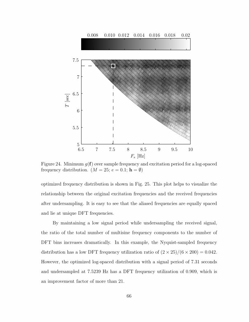
5
5.5
6
6.5
6.5
7
7
7.5
7.5 8 8.5 9 9.5 10
0.008 0.010 0.012 0.014 0.016 0.018 0.02
T[sec]
Fs [Hz]
Figure 24. Minimum g(f) over sample frequency and excitation period for a log-spacedfrequency distribution. (M = 25; e = 0.1; h = ∅)
optimized frequency distribution is shown in Fig. 25. This plot helps to visualize the
relationship between the original excitation frequencies and the received frequencies
after undersampling. It is easy to see that the aliased frequencies are equally spaced
and lie at unique DFT frequencies.
By maintaining a low signal period while undersampling the received signal,
the ratio of the total number of multisine frequency components to the number of
DFT bins increases dramatically. In this example, the Nyquist-sampled frequency
distribution has a low DFT frequency utilization ratio of (2× 25)/(6× 200) = 0.042.
However, the optimized log-spaced distribution with a signal period of 7.31 seconds
and undersampled at 7.5239 Hz has a DFT frequency utilization of 0.909, which is
an improvement factor of more than 21.
66

100
101
102
0 1 2 3 4
Analysis frequency [Hz]
Excitation
frequency
[Hz]
Nyquistrate
Figure 25. Analysis frequency vs excitation frequency for an undersampled optimizedlog-spaced frequency distribution. (Fs = 7.5239 Hz)
67

CHAPTER 6. MULTISINE SIGNAL GENERATION
6.1. Introduction
This chapter explores methods for optimizing the generation of multisine
excitation signals. A proposal is made to simplify the hardware complexity of
generating multisine signals by using multiple square wave generators rather than a
digital-to-analog converter (DAC) paired with a recursive oscillator or look-up table.
First, the properties of square waves are reviewed. Second, the requirements for
generating multiple square wave signals that are synchronous to a common system
clock are presented.
6.2. Multisquare-Multisine Generator
The traditional methods for sinusoid signal generation are not optimized for
the generation of multisine excitation signals. Whereas digital recursive oscillators
are well-equipped to generate single frequency sinusoids, a multisine signal generator
requires one digital recursive oscillator for each frequency component in the signal.
Likewise, digital recursive oscillators require a hardware architecture capable of
multiplication and addition operations at a frequency many times greater than the
maximum frequency of the multisine signal. On the other hand, look-up table signal
generators are capable of generating arbitrary waveforms and, therefore, can produce
a multisine signal. However, a multisine signal can have a relatively large signal
period compared to its sinusoid components and, thus, can require an impractical
amount of memory to store all the necessary data points needed to generate the
multisine signal with adequate resolution. Beyond the method of generating the
digital codes that represent discrete points of the generated multisine signal, these
approaches also require a high-speed and high-resolution digital-to-analog converter
(DAC) to convert the digital codes into an analog output. This DAC needs to run at
a sampling frequency at least twice the highest frequency component of the multisine
68

signal, and it requires many bits to produce the desired analog output with sufficient
resolution. In some applications of system identification, such as energy harvesting
systems, this DAC alone may be impractical to implement due to power and cost
reasons.
The objective is to exploit characteristics of multisine signals that enable the
simplification of the signal generation such that complex mathematical computations,
large memory banks, or high-speed and high-resolution DACs are not required. The
first step in simplifying the generation of multisine signals is to concentrate on the
types of signals that digital circuits are adept at producing. Considering that digital
logic circuits are specifically designed to produce ones and zeros, usually represented
as high and low voltages, a straightforward waveform to generate with a digital circuit
would be a square wave. This could be readily produced by the toggling output of
an inverter or other logic gate.
An odd-symmetry square wave can be mathematically decomposed into a
summation of harmonically related sinusoids, as shown by the Fourier series
representation
x(t) =4
π
∞∑
n=1,3,5,···
1
nsin(2πfnt). (96)
Fig. 26 illustrates a portion of the Fourier transform of a square wave with a
fundamental frequency of 1Hz. It can be seen that a square wave consists of
only frequency components that are odd-multiples of the fundamental, and that the
amplitudes of the harmonic decreases at a rate of 1/n as the frequency increases. By
eliminating all of the upper frequency components above a certain cutoff frequency,
possibly by low-pass filtering, the resulting signal looks less like an ideal square wave
and more like a single frequency sinusoid. This is shown in Fig. 27, where traces
consisting of one, two, three, four, five, and all of the harmonics of a square wave are
plotted.
69

0
0.2
0.4
0.6
1 3 5 7 9 11 13 15 17 19
|X(f)|
f [Hz]
Figure 26. Fourier transform of a square wave
0
0 0.5
1
1
−1
x(t)
t
Figure 27. Impact of square wave harmonics
Through the combination of multiple square wave generators and low-pass
filters with carefully selected cutoff frequencies, it is possible to generate a multisine
excitation signal without using any high-speed and/or high-resolution DACs, memory,
70

or complex mathematical computations. A proposed multisine signal generator is
shown in Fig. 28. The mth square wave generator is defined as
xm(t) = Amsgn [sin (2πfmt+ φm)] , (97)
where sgn(t) is the signum function
sgn(t) =
−1 for t < 0
0 for t = 0
1 for t > 0,
(98)
Am is the amplitude, fm is the frequency, and φm is the phase of xm(t). Each of theM
square wave generators is followed by a low-pass filter, hm(t) filters xm(t), to attenuate
higher order harmonics prior to summation with the other square wave generators.
Alternatively, a single low-pass filter h(t) can be used to attenuate all high frequency
content above fM , assuming xm has the greatest fundamental frequency of all of the
square wave generators. Because the multisine signal generated by this particular
architecture is derived from the summation of multiple filtered square waves, the
output signal is hereby referred to as a multisquare-multisine (MSMS) signal.
x1(t) h1(t)
x2(t) h2(t)
x3(t) h3(t)
xM(t) hM(t) h(t) x(t)
Figure 28. Block diagram of a multi-square wave signal generator
71

To minimize the hardware complexity required to generate the M square wave
signals in an MSMS generator, it is beneficial to derive all frequencies from a single
clock source using even integer dividers. For example, if the common clock source is
f0, then the frequencies f0/2, f0/4, f0/6, f0/8 and so on can be readily generated with
standard logic gates. The relation of these clocks is shown in Fig. 29. Observe that
using even integer dividers creates a clock with a 50% duty cycle that is synchronous
only to the rising edge of the common clock f0. This relationship dictates that
fm =f02km
where km ∈ {1, 2, 3, · · · }. (99)
f0
f0 /2
f0 /4
f0 /6
f0 /8
f0 /10
t
Figure 29. Timing diagram of multiple synchronous clocks derived from f0
6.3. Minf0-Targetp Algorithm
An MSMS generator can generate an endless variety of excitation signal
frequency distributions. The possible values for each frequency component in f are
dictated by Eq. (99) and the common clock frequency f0. If high excitation frequencies
are required, or if fine resolution is needed for defining the excitation frequencies, then
a high f0 may be necessary. Of course, hardware power consumption is proportional
to the clock frequency. Thus, it is desirable to keep f0 as low as possible.
An iterative Minf0-Targetp algorithm is presented here to identify an MSMS
generator excitation frequency distribution g that sufficiently approximates a target
72

excitation frequency distribution p. The primary objective of the algorithm is to
minimize the generator’s common clock frequency f0. A secondary objective of the
algorithm is to reduce the excitation signal period T to reduce the system test time.
A tertiary objective of the algorithm is to select excitation frequencies such that a
significant non-fundamental harmonic of one excitation frequency is not co-located
with a second excitation frequency. The inputs to the Minf0-Targetp algorithm
are the target frequency distribution p, the maximum allowed error e as defined in
Eq. (65), and a set of harmonics h. The set h defines the significant harmonics of
g that will remain after low-pass filtering of the square wave sources in the MSMS
generator. For example, if the low-pass filters are designed to sufficiently attenuate all
harmonics above the 7th order harmonic, then h = {3, 5, 7}. Even-order harmonics
are not included since they are not generated by the square wave sources. However,
the algorithm can support even-order harmonics, and it may be desirable to include
them in h if there is an appreciable even-order nonlinearity somewhere in the system.
Two outputs of the algorithm are a lower limit fL and an upper limit fU that define
the valid range for the minimum value of f0, where fL ≤ f0 ≤ fU . This provides
some flexibility when choosing the common clock frequency and allows for some error
and drift in the clock generation circuitry. The third output of the algorithm is a
set of clock divider coefficients k. With this information, the optimized excitation
frequency distribution g is found by
g =f02k
where fL ≤ f0 ≤ fU . (100)
Furthermore, the excitation signal period T is calculated as
T =LCM(2k)
f0, (101)
73

where LCM(x) is the least common multiple of all elements in set x.
The Minf0-Targetp algorithm repeatedly increments kM until solutions for all
other km for 1 ≤ m ≤ (M − 1) can be found. For a given value of kM , the limits for
fL and fU can be initially defined as
fL = 2kMpM(1− e) (102)
and
fU = 2kMpM(1 + e), (103)
where e is the maximum error allowed between pm and gm and is defined in Eq. (65).
In addition, the initial normalized excitation period for a given kM is defined by gM
as
Tn =1
gM=
2kMfn
, (104)
where fn = 1 Hz. The normalized excitation period Tn relates to the actual excitation
period T according to
T =Tn
f0. (105)
The algorithm operates on Tn since the exact value for f0, and therefore T , is not
known.
The subset of divisors of set k that have yet to be solved are defined as u,
where each element of u is an index to an unsolved element in k. Therefore, the set
is initially defined as u = {1, 2, 3, · · · ,M − 1)}. If a solution for k2 was to be found
next, for example, then u would become u = {1, 3, 4, · · · ,M − 1}. The search space
Suifor ui ∈ u of possible solutions to kui
can be written as
Sui=
{
x ∈ Z :
⌈
fL2pui
(1 + e)
⌉
≤ x ≤⌊
fU2pui
(1− e)
⌋}
. (106)
74

The domain Z is defined as
Z = {x : kM ≤ x ≤ max k1} (107)
where max k1 is the maximum integer value of k1 that will result in a g1 that satisfies
the error limit e. It can be written as
max k1 =
⌊
fU2p1(1− e)
⌋
. (108)
The definition of Z assumes that min g = g1.
During each iteration, the Minf0-Targetp algorithm chooses a solution for one
unsolved frequency in k. Assuming that the most recent solution chosen is km, then
the set u becomes u = u\m. The choice of km from Z also reduces the set of available
solutions for the remaining unsolved divisors in k. This is due to four reasons:
1. The most recent solution km cannot be a solution for any other element in k.
If this was not true, then two excitation frequencies would be co-located.
2. The remaining unsolved divisors in k cannot generate a fundamental frequency
that exists at the same frequency as a significant harmonics of km as defined by
set h. The set of divisors this excludes from Z is
α(km) =
x ∈ Z : x ∈|h|⋃
i=1
kmhi
. (109)
3. No harmonics of frequencies defined by the divisors in Z can be co-located with
km. The set of divisors this excludes from Z is
β(km) =
x ∈ Z : fm ∈|h|⋃
i=1
x
hi
. (110)
75
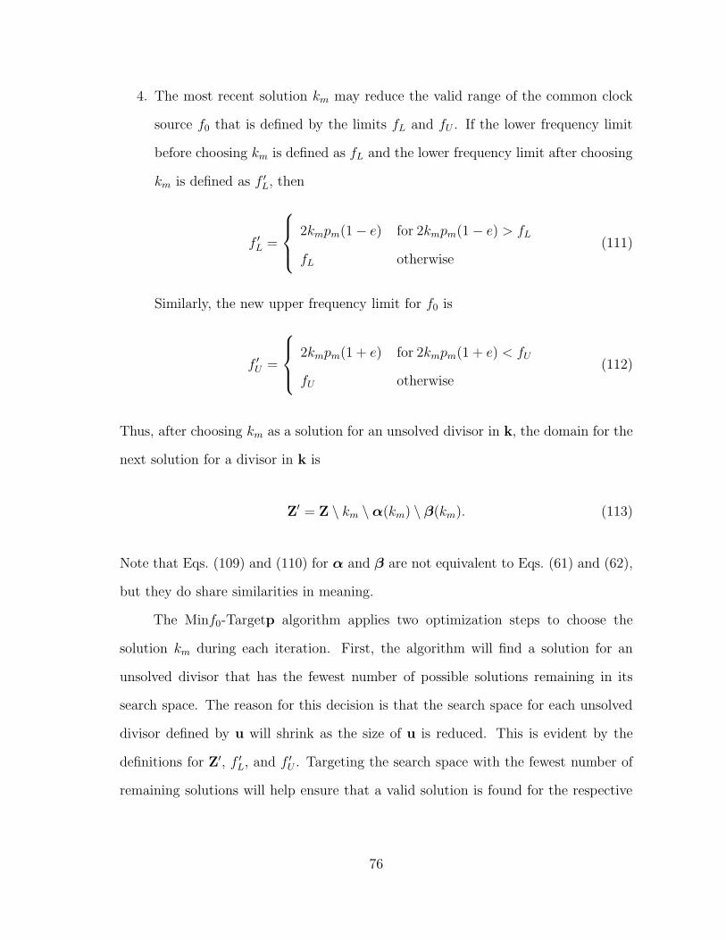
4. The most recent solution km may reduce the valid range of the common clock
source f0 that is defined by the limits fL and fU . If the lower frequency limit
before choosing km is defined as fL and the lower frequency limit after choosing
km is defined as f ′L, then
f ′L =
2kmpm(1− e) for 2kmpm(1− e) > fL
fL otherwise(111)
Similarly, the new upper frequency limit for f0 is
f ′U =
2kmpm(1 + e) for 2kmpm(1 + e) < fU
fU otherwise(112)
Thus, after choosing km as a solution for an unsolved divisor in k, the domain for the
next solution for a divisor in k is
Z′ = Z \ km \α(km) \ β(km). (113)
Note that Eqs. (109) and (110) for α and β are not equivalent to Eqs. (61) and (62),
but they do share similarities in meaning.
The Minf0-Targetp algorithm applies two optimization steps to choose the
solution km during each iteration. First, the algorithm will find a solution for an
unsolved divisor that has the fewest number of possible solutions remaining in its
search space. The reason for this decision is that the search space for each unsolved
divisor defined by u will shrink as the size of u is reduced. This is evident by the
definitions for Z′, f ′L, and f ′
U . Targeting the search space with the fewest number of
remaining solutions will help ensure that a valid solution is found for the respective
76

divisor before all valid solutions are eliminated. Thus, m ∈ q, where
q = argmini∈u
|Si| (114)
and Si is found with Eq. (106). Likewise, km ∈ b, where
b =
|q|⋃
i=1
Sqi. (115)
The second optimization step chooses the solution km from b that minimizes
the increase to the signal excitation period T . If the normalized excitation period
before choosing km is Tn and the normalized excitation period after choosing km is
T ′n, then
T ′n = LCM(Tn, 2km). (116)
Therefore, the algorithm chooses km to be
km = argminx∈b
(LCM(Tn, 2x)) , (117)
where
m = {x ∈ q : km ∈ Sx} . (118)
The complete Minf0-Targetp algorithm is described in pseudo-code. The
objective is to minimize kM , thereby also minimizing f0.
1. Start with kM = 1.
2. Find fL, fU , Tn, and Z with Eqs. (102), (103), (104), and (107), respectively.
3. Define u = {1, 2, 3, · · · ,M − 1} so solutions to all divisors except for kM will
be found. M is not included in u since a solution for KM is assumed.
77

4. Substitute Z′ for Z based on the value of kM .
5. Apply Eqs. (117) and (118) to find a solution for one km in k, where m ∈ u. If
the set of possible solutions Suifor any kui
is empty, then increment kM and go
to step 2.
6. Update the set of unsolved divisors to u′ = u\m. If u′ = ∅, then the algorithm
is complete, fL = f ′L, and fU = f ′
U .
7. Use Eq. (113) to update the search domain. If Z′ = ∅, increment kM and go
back to step 2.
8. Substitute f ′L for fL, f
′U for fU , Z
′ for Z, T ′n for Tn and u′ for u and return to
step 5.
6.3.1. Numerical Example
Consider the example where p = {10, 20, 50} Hz, h = ∅, and e = 0.1. The
algorithm begins with kM = 1. Step 2 of the algorithm calculates the initial values
of fL = 90 Hz, fU = 110 Hz, Tn = 2 seconds and Z = {1, 2, 3, 4, 5, 6}. In steps 3 and
4, the solution for kM is initially assumed to be 1. This results in u = {1, 2} and
Z′ = {2, 3, 4, 5, 6}.
Next, the search spaces S1 = {5, 6} and S2 = {3} for the two elements in u are
found. k2 has fewer potential solutions than k1 because S2 has fewer elements than
S1. This results in q = {2}, and b = {3}. The first application of Eq. (117) gives
km = 3, and Eq. (118) gives m = 2. Thus, k2 = 3.
After finding a solution for k2, the set of unsolved divisors becomes u = {1}.
Likewise, Z′ = {2, 4, 5, 6}, f ′L = 108 Hz, f ′
U = 110 Hz, and T ′n = 6 seconds. The search
space for k1 remains unchanged. Applying Eqs. (117) and (118) on the updated values
for fL, fU , Z, and Tn results in k1 = 6. Thus, the final solution for k is k = {6, 3, 1}.
The frequency range for f0 remains at 108 ≤ f0 ≤ 110 Hz.
78

6.4. Algorithm Application
The Minf0-Targetp algorithm is applied to the same target excitation
distribution p used throughout this paper. It is defined as a logarithmically-spaced
distribution ranging from p1 = 1 Hz to pM = 100 Hz and is composed of M = 25
tones. The resulting minimum source frequency fL is plotted in Fig. 30 against e/emax,
where emax is defined in Eq. (93). It is observed that fL has only a weak dependency
on the number of significant odd harmonics, at least for the values of h evaluated.
This suggests that it may be advantageous to optimize the excitation distribution
using a larger set of harmonics in h in order to relax the requirements of the low-pass
filters needed to remove the higher frequency harmonics. However, Fig. 31 tells a
different story. In this plot it is shown that the excitation signal period T can have
a strong dependency on the number of harmonics in h. For example, it is possible to
obtain T = 5.4 seconds for h = {}, but this increases to T = 356 seconds for h = {3}
and h = {3, 5}. Depending on the application requirements, this significant increase
in excitation signal period may or may not be acceptable.
To better understand the dependency of the Minf0-Targetp algorithm on the
number of tones in p, the target excitation distribution is modified from M = 25
to M = 11. It is still logarithmically-spaced with p1 = 1 Hz and pM = 100 Hz.
The expectation is that reducing the number of tones in p will reduce fL and T for a
given e/emax and h since there will be fewer harmonic frequencies that the algorithm
will need to accommodate. The algorithm results are plotted in Figs. 32 and 33
and significant improvements compared to the M = 25 case are readily apparent.
Observe that even for h = {3, 5, 7, 9, 11}, an excitation period of T = 4.9 seconds
can be achieved with a common source frequency of f0 = (fU + fL)/2 = 389 Hz.
Furthermore, this optimization point is found for a value of e/emax just less than 0.5,
and is even better than values of e closer to emax. It is worth noting that increasing
79

0
0.2 0.4 0.6 0.8 1500
1000
1500
2000
2500
3000
3500
4000
f L[H
z]
e/emax
h = [3, 5, 7, 9, 11]h = [3, 5, 7, 9]h = [3, 5, 7]h = [3, 5]h = [3]h = []
Figure 30. fL vs e/emax and h using the Minf0-Targetp algorithm for p1 = 1, pM =100, and M = 25.
0
0.2 0.4 0.6 0.8 1
101
103
105
107
109
1011
T[sec]
e/emax
h = [3, 5, 7, 9, 11]h = [3, 5, 7, 9]h = [3, 5, 7]h = [3, 5]h = [3]h = []
Figure 31. T vs e/emax and h using the Minf0-Targetp algorithm for p1 = 1, pM =100, and M = 25.
80

e does not always lead to a better solution as one may expect. This is due to the
iterative structure of the algorithm which must solve for values of k prior to realizing
all ramification on the final result.
0
0.2 0.4 0.6 0.8 1200
300
400
500
600
700
800
900
1000
1100f L
[Hz]
e/emax
h = [3, 5, 7, 9, 11]h = [3, 5, 7, 9]h = [3, 5, 7]h = [3, 5]h = [3]h = []
Figure 32. fL vs e/emax and h using the Minf0-Targetp algorithm for p1 = 1, pM =100, and M = 11.
The results obtained in Figs. 32 and 33 show that it is quite possible to
generate an MSMS signal with a reasonable excitation period and using a system clock
frequency that is only a few times greater than the maximum excitation frequency.
All of this is achieved while simultaneously selecting the square wave frequencies
such that there is no distortion from the 3rd through 11th order harmonics of any
fundamental excitation frequencies. Assuming that the 13th order harmonics do
result in distortion, then filtering each square wave generater xi(t) with a low pass
filter hi(t), as shown in Fig. 28, can attenuate the 13th order harmonics below the
noise floor in many applications. For example, if hi(t) is a third order Butterworth
low pass filter with a -3dB cutoff point at the fundamental frequency of xi(t), then
the resulting xi(t) ∗ hi(t) signal will closely approximate a pure sinusoid, as shown
81

0
0.2 0.4 0.6 0.8 1100
101
102
103
T[sec]
e/emax
h = [3, 5, 7, 9, 11]h = [3, 5, 7, 9]h = [3, 5, 7]h = [3, 5]h = [3]h = []
Figure 33. T vs e/emax and h using the Minf0-Targetp algorithm for p1 = 1, pM = 10,and M = 11.
in Fig. 34. Converting this to the frequency domain, as shown in Fig. 35, illustrates
that this is sufficient to suppress the 13th order harmonic to about 88 dB below the
fundamental frequency of xi(t) after filtering.
6.5. Crest Factor Optimization
Several methods exist for manipulating the phases of a multisine excitation
signal in order to optimize the crest factor. A low crest factor is beneficial as it
improves the signal-to-noise ratio of the measurement, can reduce the severity of some
system nonlinearities, and decreases the test time by allowing for an excitation signal
with increased signal power for a given peak amplitude. Unfortunately, these existing
techniques may not be directly applicable to signals produced by a multisquare-
multisine signal generator. Because all tones in an MSMS signal are derived from
a common clock source using integer dividers, all frequency tones obey a strict phase
relationship. Only a discrete set of phases is possible for each tone of the signal. The
crest factor optimization algorithm is not free to operate over the continuum of phase.
82

−1
0
1
0 T
Magnitude
t [sec]
x1(t)x1(t) ∗ h1(t)
Figure 34. Time domain plot for a square wave [x1(t)] and a low-pass filtered squarewave [x1(t) ∗ h1(t)]. The low-pass filter has a third-order Butterworth response witha -3 dB cut-off point at the fundamental.
Presented here is one method to optimize the crest factor of an MSMS signal
through the assignment of phase to each tone in the distribution. For a given tone gm
that is derived from a common clock f0 with a divider of 2km as shown in Eq. (99),
the set of valid phases for gm is
θm = 2πn
2kmfor n = {1, 2, 3, · · · , 2km}. (119)
This is illustrated in Fig. 36 for km = 2. Notice that f0/4 can be shifted in time in
increments equal to the period of f0, and that the edges of f0/4 remain aligned with
the rising edges of f0.
The set of available phases for gm grows as km increases. Thus, high frequency
tones have less phase resolution compared to low frequency tones for a given source
frequency f0. This observation forms the basis for the crest factor optimization
algorithm proposed here. It is an iterative algorithm that optimizes the phase of one
83

0
−25
−50
−75
−100
−125
1 3 5 7 9 11 13 15 17 19 21
Magnitude[dB]
Harmonic
x1(t)x1(t) ∗ h1(t)
Figure 35. FFT plot for a square wave [x1(t)] and a low-pass filtered square wave[x1(t) ∗ h1(t)]. The low-pass filter has a third-order Butterworth response with a -3dB cut-off point at the fundamental. The filtered 13th harmonic is 88 dB less thanthe filtered fundamental.
f0
f0/4
f0/4 + 3π/2
f0/4 + π/2
f0/4 + π
t
Figure 36. Phases of f0/4 that can be generated from f0
frequency component gm in x(t) at a time by choosing the phase from set φm that
minimizes the signal crest factor. The algorithm starts with the highest frequency
component gM and works towards the lowest frequency component g1. This ordering
provides increasing flexibility in tuning the phase of a frequency component as the
power of the signal increases. This is evident in the pseudo-code provided here.
84

1. Start with m = M .
2. Choose the phase φm for xm from φm according to
φm = argminx∈θm
CR
(
M∑
i=m
xi(t) ∗ hi(t)
)
(120)
where CR(x) is defined in Eq. (20) and
xi(t) = Aisgn [sin (2πgit+ φi)] . (121)
3. Decrement m and return to step 1 until the phases for all M components are
found.
The capabilities of the phase optimization algorithm are demonstrated by
comparing the algorithm result to the crest factors of random phase assignments
and an equal phase assignment. An equal phase assignment is defined as φm = φm+1
for 0 ≤ m ≤ M−1. The crest factor of a random phase assignment is calculated 1000
times and displayed as a histogram in Fig. 37 to show the approximate probability
distribution function of random phase assignment. The random phases were selected
from the set of phases φm defined in Eq. (119) to restrict them to only the discrete
phases that can be produced by the proposed MSMS signal generator. The results are
calculated for an excitation distribution produced by the Minf0-Targetp algorithm
for a target logarithmically-spaced frequency distribution p where p1 = 1, pM = 100,
and M = 25. The set of accommodated harmonics is h = {3, 5, 7, 9, 11}. The results
for this specific test case show that the crest factor for randomly assigned phase has
an approximate Gaussian distribution with a mean of about 3.3. The optimization
algorithm produced a crest factor of 2.77 that is about 2 standard deviations below
85

the random phase mean. The equal phase assignment produced a crest factor that is
1.9 standard deviations greater than the random phase mean.
2.5 3 3.5 4 4.50
50
100
150
200
Crest Factor
Cou
nts
Mean
Algorithm
Optimized
Phases
Equal
Phases
Figure 37. Crest factor histogram for random discrete phases for p1 = 1, pM = 100,M = 11, f0 = 389 Hz, and T = 4.9 seconds.
The exercise is repeated using continuous random variables for the phase in
order to better understand the limitations imposed by discrete phase assignment.
The resulting histogram is shown in Fig. 38. Both the mean and the standard
deviation of the resulting crest factor probability distribution function are similar
to the discrete phase results. Thus, the limitation of discrete phases does not appear
to have a significant negative impact on the signal crest factor when using random
phase assignment. However, the crest factor optimization algorithm presented here
still offers a significant benefit when compared to random phase assignment or equal
phase assignment.
86
2.5 3 3.5 4 4.50
50
100
150
200
Crest Factor
Cou
nts
Mean
Algorithm
Optimized
Phases
Equal
Phases
Figure 38. Crest factor histogram for random continuous phases for p1 = 1, pM = 100,M = 11, f0 = 389 Hz, and T = 4.9 seconds.
87
CHAPTER 7. FUTURE WORK & CONCLUSIONS
Two primary techniques are presented in this paper for reducing the complexity
and power consumption of system identification hardware through optimization of
the multisine excitation signal. The proposed improvements attack both ends of the
signal chain, excitation signal generation and system output analysis. The focus
of the research is on the selection of the frequency tones that comprise a multisine
excitation signal such that power saving architectures and signal processing techniques
can be employed without significantly distorting the generated excitation signal or
the sampled output signal.
Hardware complexity and system power consumption are potentially reduced
at the signal generation end of the signal chain by using low complexity square
wave generators and low-pass filters to create a multisine signal from a summation of
square wave signals. To deal with the significant odd harmonics that are created by
square wave signals, the iterative Minf0-Targetp algorithm is proposed to optimize the
selection of square wave fundamental frequencies such that the generated harmonic
tones do not distort the excitation tones of interest. Examples provided for sparse
logarithmically-spaced frequency distributions show that distortion from odd-order
harmonics up to the 11th order or more can be achieved without significantly
increasing the required excitation sample period. Furthermore, this can be achieved
while requiring a system clock frequency that is only three to four times greater than
the maximum frequency component of the multisine signal. Lastly, results show that
it is possible to significantly improve the crest factor of an optimized multisine signal
that is composed of multiple square waves.
The MinN -Targetp algorithm is proposed for decreasing the system complexity
and power consumption required to sample and analyze the system output signal in
a system identification application. The improvements are realized by designing a
88

multisine excitation signal such that it can be undersampled without distorting any
of the excitation frequencies. This has the effect of compacting a sparse excitation
frequency distribution into a more dense distribution, thereby increasing the DFT
bin utilization. The efficiency of many DFT algorithms is generally improved when
the total number of DFT bins is reduced. Similar to the Minf0-Targetp algorithm,
the MinN -Targetp algorithm is also designed to accommodate a select number of
harmonic components. This makes it possible to undersample the system output
signal without distortion even if the system under test includes a significant nonlinear
component. Multiple search operators for the MinN -Targetp algorithm are proposed,
and examples for a typical logarithmically-spaced excitation signal show that it is
possible to improve the DFT bin utilization by more than one order of magnitude.
Analyzing the performance of the Minf0-Targetp and MinN -Targetp algorithms
when applied to a more diverse set of target excitation frequencies is a warranted
exercise. Logarithmically-spaced frequency distributions are commonly used in
system identification applications, but the number of tones and the frequency range
can vary greatly. Likewise, the expected order of the system nonlinearity and the
required excitation signal period further impact results. Fortunately, the presented
algorithms do not have any inherent limitations that prevent them from operating on
an arbitrarily defined target frequency distribution or set of harmonic components.
Another interesting exercise would be to combine the Minf0-Targetp and MinN -
Targetp algorithms such that a single excitation signal could be designed such
that it could be produced by a summation of square wave generators and also be
undersampled without distortion. This combination of objectives places additional
boundaries on the algorithm search space, therefore it is expected that the results
will be inferior compared to excitation signal optimization using only the generation
or analysis optimization algorithm. Still, there may be advantages to applying both
89

algorithms at once, depending on the instrumentation hardware and the measurement
application.
A very large, yet important, future undertaking would be to realize the benefits
of the two proposed algorithms in actual hardware. One such application could
be a single integrated-circuit instrumentation platform for SHM that incorporates a
simplified multisquare-multisine signal generator. Applying the DFT bin utilization
improvements of the MinN -Targetp algorithms will potentially reduce the memory
depth and operating frequency requirements of the signal analysis hardware in the
single chip solution. Implementing the improvements offered by the optimization
algorithms in actual hardware will provide the best true indication of the power and
cost savings that can be achieved. The results presented in this dissertation are
theoretical only and indicate the potential magnitude of improvement that may be
obtained.
90

REFERENCES
[1] J. Kim et al., “A system-on-board approach for impedance-based structural
health monitoring,” Proc. of SPIE, vol. 6529, Mar 19, 2007.
[2] T. Overly et al., “Development of an extremely compact impedance-based
wireless sensing device,” Smart Materials and Structures, vol. 17, no. 6, Dec
2008.
[3] S. Wag et al., “0.18 µm cmos integrated circuit design for impedance-based
structural health monitoring,” Circuits, Devices Systems, IET, vol. 4, no. 3, pp.
227 –238, May 2010.
[4] M. Lallart et al., “Energy-efficient method for embedded in situ structural health
monitoring,” Structural Health Monitoring, vol. 9, no. 1, pp. 87–98, Jan 2010.
[5] K. Farinholt et al., “Energy harvesting and wireless energy transmission for
embedded shm sensor nodes,” Structural Health Monitoring, vol. 9, no. 3, pp.
269–280, May 2010.
[6] D. Mascarenas et al., “Experimental studies of using wireless energy transmission
for powering embedded sensor nodes,” Journal of Sound and Vibration, vol. 329,
pp. 2421–2433, 2010.
[7] G. Park et al., “Energy harvesting for structural health monitoring sensor
networks,” Journal of Infrastructure Systems, vol. 14, no. 1, pp. 64–79, Mar
2008.
[8] K. Roy et al., “Leakage current mechanisms and leakage reduction techniques
in deep-submicrometer cmos circuits,” Proceedings of IEEE, vol. 91, no. 2, pp.
305–327, Feb 2003.
91

[9] A. Wang & A. Chandrakasn, “A 180-mv subthreshold fft processor using a
minimum energy design methodology,” IEEE Journal of Solid-State Circuits,
vol. 40, no. 1, pp. 310–319, Jan 2005.
[10] S. Sridhara et al., “Microwatt embedded processor platform for medical system-
on-chip applications,” IEEE Journal of Solid-State Circuits, vol. 46, no. 4, pp.
721–730, Apr 2011.
[11] J. Liang & D. Johns, “A frequency-scalable 15-bit incremental adc for low power
sensor applications,” Proceedings of 2010 IEEE International Symposium on
Circuits and Systems (ISCAS), pp. 2418 –2421, Jun 2010.
[12] I. Ahmed & D. Johns, “A 50ms/s (35mw) to 1ks/s (15µw) power scaleable 10b
pipelined adc with minimal bias current variation,” IEEE International Solid-
State Circuits Conference, pp. 280, 281, 598, Feb 2005.
[13] T. Dudykevych et al., “Impedance analyser module for eit and sepctroscopty
using undersampling,” Physiological Measurement, vol. 22, pp. 19–24, Feb 2001.
[14] Gamry Instruments, “Sub-harmonic sampling for electrochemical impedance
spectroscopy,” http://www.gamry.com.
[15] A. Hartov et al., “A multichannel continuously selectable multifrequency
electrical empedance spectroscopy measurement system,” IEEE Trans. on
Biomedical Engineering, vol. 47, no. 1, pp. 49–58, Jan 2000.
[16] O. Martens & M. Min, “Multifrequency Bio-Impedance Measurement:
Undersampling Approach.” Proc. 6th Nordic Signal Processing Symposium.
NORSIG 2004, 2004, pp. 145–148.
92

[17] J. Shoukens et al., “Broadband versus stepped sine frf measurements,” IEEE
Trans. on Instrumentation and Measurement, vol. 49, no. 2, pp. 275–278, Apr
2000.
[18] S.C. Creason, D.E. Smith, “Fourier transform faradaic admittance measurements
ii. ultra-rapid, high precision acquisition of the frequency response profile,” J.
Electroanal. Chem., vol. 40, pp. A1–A5, 1972.
[19] S.C. Creason, J.W. Hayes, D.E. Smith, “Fourier transform faradaic admittance
measurements iii. comparison of measurement efficiency for various test signal
waveforms,” J. Electroanal. Chem., vol. 47, pp. 9–46, 1973.
[20] C. Evans & D. Rees, “Nonlinear distortions and multisine signals - part i:
Measureing the best linear approximation,” IEEE Trans. on Instrumentation
and Measurement, vol. 49, no. 3, pp. 602–609, Jun 2000.
[21] ——, “Nonlinear distortions and multisine signals - part ii: Minimizing the
distortion,” IEEE Trans. on Instrumentation and Measurement, vol. 49, no. 3,
pp. 610–616, Jun 2000.
[22] M. Schmitz & R. Green, “Optimization of Multisine Excitations for Receiver
Undersampling.” Dallas, TX: IEEE International Conference on Acoustics,
Speech, and Signal Processing, March, 2010.
[23] T. Breugelmans et al., “Odd random phase multisine eis as a detection method
for the onset of corrosion of coated steel,” Electrochemistry Communications,
vol. 12, pp. 2–5, 2010.
[24] O. Blajiev et al., “Detection and evaluation of measurement noise and
stochastic non-linear distortions in electrochemical impedance measurements by
93

a model based on a broadband periodic excitation,” Journal of Elecroanalytical
Chemistry, vol. 576, pp. 65–72, 2005.
[25] E. Van Gheem et al., “Electrochemical impedance spectroscopy in the presence
of non-linear distortions and non-stationary behaviour part i: Theory and
validation,” Electrochimica Acta, vol. 49, pp. 4753–4762, 2004.
[26] G. Popkirov & R. Schindler, “Effect of sample nonlinearity of the performance
of time domain electrochemical impedance spectroscopy,” Electrochimica Acta,
vol. 40, no. 15, 1995.
[27] C. Evans et al., “Nonlinear disturbance errors in system identification using
multisine test signals,” IEEE Trans. on Instrumentation and Measurement,
vol. 43, no. 2, pp. 238–244, Apr 1994.
[28] K. Vanhoenacker & J. Schoukens, “Frequency response function measurements
in the presence of nonlinear distortions.” IEEE International Workshop on
Intelligent Signal Processing, Sept 4-7, 1999, pp. 87–92.
[29] M. Schmitz & R. Green, “Multisine Excitation Design to Increase the
Efficiency of System Identification Analysis through Undersampling and DFT
Optimization,” Measurement, vol. 45, no. 6, pp. 1576–1586, Jul 2012.
[30] R. Muller, “The cathode ray-tube polarograph,” Industrial & Engineering
Chemistry Analytical Edition, vol. 10, no. 6, pp. 339–341, Jun 1938.
[31] D. Grahame, “Properties of the electrical double layer at a mercury surface. i.
methods of measurements and interpretation of results,” Journal of the American
Chemical Society, vol. 63, no. 5, pp. 1207–1215, May 1941.
94

[32] ——, “Properties of the electrical double layer at a mercury surface. ii. the effect
of frequency on the capacity and resistance of ideal polarized electrodes,” Journal
of the American Chemical Society, vol. 68, no. 2, pp. 301–310, Feb 1946.
[33] ——, “The electrical double layer and the theory of electrocapillarity,” Chemical
Reviews, vol. 41, no. 3, pp. 441–501, Dec 1947.
[34] Q. Le Thu et al., “Eis and enm measurements for three different organic coatings
on aluminum,” Progress in Organic Coatings, vol. 42, no. 3-4, pp. 179–187, Sept
2001.
[35] G. Bierwagen et al., “Eis studies of coated metals in accelerated exposure,”
Progress in Organic Coatings, vol. 46, no. 2, pp. 149–158, Mar 2003.
[36] A. Ciubotariu et al., “Electrochemical impedance spectroscopy and corrosion
behaviour of al2o3 - ni nano composite coatings,” Electrochimica Acta, vol. 53,
no. 13, pp. 4557–4563, May 2008.
[37] E. McAdams & J. Jossinet, “Tissue impedance: A historical overview,”
Physiological Measurement, vol. 16, pp. A1–A13, Aug 1995.
[38] B. Rigaud et al., “In vitro tissue characterization and modelling using electrical
impeance measurements in teh 100 hz - 10 mhz frequency range,” Physiological
Measurement, vol. 16, pp. A15–A28, Aug 1995.
[39] G. Instruments, “Reference 600 brochure,” Available at http://www.gamry.com.
[40] K. Salloux, “Eliminating Battery Failure - Two New Leading Indicators of
Battery Health: A Case Study,” Presentation at Battery Power 2007, Denver,
CO, June 2007.
95

[41] R. Pintelon & J. Schoukens, System Identification: A Frequency Domain
Approach. IEEE Press, 2001.
[42] A. McCormack et al., “The suppression of drift and transient effects
for frequency-domain identification,” IEEE Trans. on Instrumentation and
Measurement, vol. 43, no. 2, pp. 232–237, Apr 1994.
[43] J. Cooley & J. Tukey, “An algorithm for the machine calculation of complex
fourier series,” Mathematics of Computation, vol. 19, no. 90, pp. 297–301, Apr
1965.
[44] J. Shoukens et al., “Survey of excitation signals for fft based signal analyzers,”
IEEE Trans. on Instrumentation and Measurement, vol. 37, no. 3, pp. 342–352,
Sept 1988.
[45] E. Van der Ouderaa et al., “Peak factor minimization using a time-
frequency domain swapping algorithm,” IEEE Trans. on Instrumentation and
Measurement, vol. 37, no. 1, pp. 145–147, Mar 1988.
[46] ——, “Peak factor minimization of input and output signals of linear systems,”
IEEE Trans. on Instrumentation and Measurement, vol. 37, no. 2, pp. 207–212,
Jun 1988.
[47] E. Van der Ouderaa & J. Renneboog, “Logtone crest factors,” IEEE Trans. on
Instrumentation and Measurement, vol. 37, no. 4, pp. 656–657, Dec 1988.
[48] P. Guillaume, “Crest-factor minimization using nonlinear chebyshev
approximation methods,” IEEE Trans. on Instrumentation and Measurement,
vol. 40, no. 6, pp. 982–989, Dec 1991.
96

[49] M. R. Schroeder, “Synthesis of low-peak-factor signals and binary sequences
with low autocorrelation,” IEEE Trans. on Information Theory, vol. 16, no. 1,
pp. 85–89, Jan 1970.
[50] R. Green et al., “DSP-Based EIS Instrument Utilizing Low Peak-Factor Pseudo-
Logarithmically Spaced Multi-Frequency Test Signals,” Presentation at 207th
ECS Meeting. Impedance Based Sensors, May 2005.
[51] H. Von Bank, “”dsp-based electrochemical impedance spectroscopy”,” Thesis
Draft. Unpublished. North Dakota State University, Jan 2005.
[52] C. Shannon, “Communications in the presence of noise,” Proceedings of the IRE,
vol. 37, pp. 10–21, Jan 1949.
[53] G. Hill, “The Benefits of Undersampling,” Electronic Design, pp. 69–79, July
1994.
[54] P. Pejovic et al., “Computations of average values of synchronously sampled
signals,” IEE Proceedings of Electric Power Applications, vol. 149, no. 3, pp.
217–222, May 202.
[55] K. Ross & C. Wright, Discrete Mathematics, 4th ed. Prentice Hall, 1999.
97
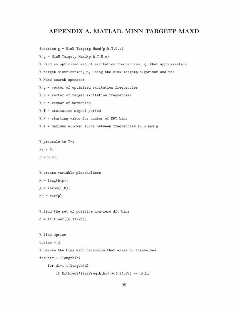
APPENDIX A. MATLAB: MINN TARGETP MAXD
function g = MinN_Targetp_Maxd(p,h,T,N,e)
% g = MinN_Targetp_Maxd(p,h,T,N,e)
% Find an optimized set of excitation frequencies, g, that approximate a
% target distribution, p, using the MinN-Targetp algorithm and the
% Maxd search operator
% g = vector of optimized excitation frequencies
% p = vector of target excitation frequencies
% h = vector of harmonics
% T = excitation signal period
% N = starting value for number of DFT bins
% e = maximum allowed error between frequencies in p and g
% prescale to T=1
Fs = N;
p = p.*T;
% create variable placeholders
M = length(p);
g = zeros(1,M);
pM = max(p);
% find the set of positive non-zero dft bins
d = (1:floor((N-1)/2));
% find dprime
dprime = d;
% remove the bins with harmonics that alias to themselves
for hi=1:1:length(h)
for di=1:1:length(d)
if ExtFreq2AliasFreq(h(hi).*d(di),Fs) == d(di)
98

dprime = setdiff(dprime, d(di));
end
end
end
% define the vector of unsolved frequencies
u = 1:1:M;
while(1)
% stop if out of DFT bins
if isempty(dprime)
g = [];
return;
end
%build the total search space
gmax = (1+e).*pM;
Z = AliasFreq2ExtFreq(dprime,Fs,gmax);
% build the search space Sm for each unsolved frequency defined in u
clear S
b = [];
for i=1:1:length(u)
freqdev = abs((Z - p(u(i)))./p(u(i)));
S{u(i)} = Z(freqdev <= e);
% stop if a search space is empty
if isempty(S{u(i)})
g = [];
return;
end
b = union(b,ExtFreq2AliasFreq(S{u(i)},Fs));
end
99

% find set c that minimizes dft usage
NumPollutedBins = [];
for x=1:1:length(b)
% find alpha
alpha = [];
for hi=1:1:length(h)
alpha = union(ExtFreq2AliasFreq(h(hi).*b(x),Fs),alpha);
end
alpha = intersect(dprime,alpha);
% find beta
beta = [];
for i=1:1:length(dprime)
for hi=1:1:length(h)
if ExtFreq2AliasFreq(h(hi).*dprime(i),Fs) ==...
ExtFreq2AliasFreq(b(x),Fs);
beta = union(dprime(i),beta);
end
end
end
PollutedBins = union(ExtFreq2AliasFreq(b(x),Fs),alpha);
PollutedBins = union(PollutedBins,beta);
NumPollutedBins(x) = length(PollutedBins);
end
MinNumPollutedBins = min(NumPollutedBins);
c = [];
for i=1:1:length(b)
if NumPollutedBins(i) == MinNumPollutedBins
c = union(b(i),c);
end
end
100

%build the total serch space using c only
gmax = (1+e).*pM;
Zprime = AliasFreq2ExtFreq(c,Fs,gmax);
% find gm
error = [];
for x=1:1:length(Zprime)
for y=1:1:length(u)
error = cat(2,error,abs((Zprime(x) - p(u(y)))./p(u(y))));
end
end
[errormin errormini] = min(error);
gm = Zprime(ceil(errormini./length(u)));
%find m
error = [];
for i = 1:1:length(u)
error(i) = abs((gm-p(u(i)))./p(u(i)));
end
[errormin m] = min(error);
% store to final freq list
g(u(m)) = gm;
% update the list of unsolved frequencies
u = setdiff(u,u(m));
% stop if all the tones have been found
if isempty(u)
% post-scale the distribution
101

g = g./T;
return;
end
% find dprimeprime
% find alpha
alpha = [];
for hi=1:1:length(h)
alpha = union(ExtFreq2AliasFreq(h(hi).*gm,Fs),alpha);
end
alpha = intersect(dprime,alpha);
% find beta
beta = [];
for i=1:1:length(dprime)
for hi=1:1:length(h)
if ExtFreq2AliasFreq(h(hi).*dprime(i),Fs) ==...
ExtFreq2AliasFreq(gm,Fs)
beta = union(dprime(i),beta);
end
end
end
dprimeprime = setdiff(dprime,ExtFreq2AliasFreq(gm,Fs));
dprimeprime = setdiff(dprimeprime,alpha);
dprimeprime = setdiff(dprimeprime,beta);
% substitue dprimeprime for dprime
dprime = dprimeprime;
end
102

APPENDIX B. MATLAB: MINN TARGETP MAXD MINS
function g = MinN_Targetp_Maxd_MinS(p,h,T,N,e)
% g = MinN_Targetp_Maxd_MinS(p,h,T,N,e)
% Find an optimized set of excitation frequencies, g, that approximate a
% target distribution, p, using the MinN-Targetp algorithm and the
% Maxd-MinS search operator
% g = vector of optimized excitation frequencies
% p = vector of target excitation frequencies
% h = vector of harmonics
% T = excitation signal period
% N = starting value for number of DFT bins
% e = maximum allowed error between frequencies in p and g
% prescale to T=1
Fs = N;
p = p.*T;
% create variable placeholders
M = length(p);
g = zeros(1,M);
pM = max(p);
% find the set of positive non-zero dft bins
d = (1:floor((N-1)/2));
% find dprime
dprime = d;
% remove the bins with harmonics that alias to themselves
for hi=1:1:length(h)
for di=1:1:length(d)
if ExtFreq2AliasFreq(h(hi).*d(di),Fs) == d(di)
103

dprime = setdiff(dprime, d(di));
end
end
end
% define the vector of unsolved frequencies
u = 1:1:M;
while(1)
% stop if out of DFT bins
if isempty(dprime)
g = [];
return;
end
%build the total search space
gmax = (1+e).*pM;
Z = AliasFreq2ExtFreq(dprime,Fs,gmax);
% build the search space Sm for each unsolved frequency defined in u
clear S
b = [];
for i=1:1:length(u)
freqdev = abs((Z - p(u(i)))./p(u(i)));
S{u(i)} = Z(freqdev <= e);
% stop if a search space is empty
if isempty(S{u(i)})
g = [];
return;
end
b = union(b,ExtFreq2AliasFreq(S{u(i)},Fs));
end
104

% find set c that minimizes dft usage
NumPollutedBins = [];
for x=1:1:length(b)
% find alpha
alpha = [];
for hi=1:1:length(h)
alpha = union(ExtFreq2AliasFreq(h(hi).*b(x),Fs),alpha);
end
alpha = intersect(dprime,alpha);
% find beta
beta = [];
for i=1:1:length(dprime)
for hi=1:1:length(h)
if ExtFreq2AliasFreq(h(hi).*dprime(i),Fs) ==...
ExtFreq2AliasFreq(b(x),Fs);
beta = union(dprime(i),beta);
end
end
end
PollutedBins = union(ExtFreq2AliasFreq(b(x),Fs),alpha);
PollutedBins = union(PollutedBins,beta);
NumPollutedBins(x) = length(PollutedBins);
end
MinNumPollutedBins = min(NumPollutedBins);
c = [];
for i=1:1:length(b)
if NumPollutedBins(i) == MinNumPollutedBins
c = union(b(i),c);
end
end
105

% find set k
k = [];
for i=1:1:length(u)
if intersect(ExtFreq2AliasFreq(S{u(i)},Fs),c) ~= 0
k = union(u(i),k);
end
end
% find set q
clear Ssize
q = [];
for i=1:1:length(k)
Ssize(i) = length(S{k(i)});
end
Smin = min(Ssize);
for i=1:1:length(k)
if Ssize(i) == Smin
q = union(k(i),q);
end
end
%build the total serch space using c only
gmax = (1+e).*pM;
Zprime = AliasFreq2ExtFreq(c,Fs,gmax);
% find gm
error = [];
for x=1:1:length(Zprime)
for y=1:1:length(q)
error = cat(2,error,abs((Zprime(x) - p(q(y)))./p(q(y))));
end
106

end
[errormin errormini] = min(error);
gm = Zprime(ceil(errormini./length(q)));
%find m
error = [];
for i = 1:1:length(q)
error(i) = abs((gm-p(q(i)))./p(q(i)));
end
[errormin m] = min(error);
% store to final freq list
g(q(m)) = gm;
% update the list of unsolved frequencies
u = setdiff(u,q(m));
% stop if all the tones have been found
if isempty(u)
% post-scale the distribution
g = g./T;
return;
end
% find dprimeprime
% find alpha
alpha = [];
for hi=1:1:length(h)
alpha = union(ExtFreq2AliasFreq(h(hi).*gm,Fs),alpha);
end
alpha = intersect(dprime,alpha);
% find beta
107

beta = [];
for i=1:1:length(dprime)
for hi=1:1:length(h)
if ExtFreq2AliasFreq(h(hi).*dprime(i),Fs) ==...
ExtFreq2AliasFreq(gm,Fs)
beta = union(dprime(i),beta);
end
end
end
dprimeprime = setdiff(dprime,ExtFreq2AliasFreq(gm,Fs));
dprimeprime = setdiff(dprimeprime,alpha);
dprimeprime = setdiff(dprimeprime,beta);
% substitue dprimeprime for dprime
dprime = dprimeprime;
end
108

APPENDIX C. MATLAB: MINN TARGETP MINS MAXD
function g = MinN_Targetp_MinS_Maxd(p,h,T,N,e)
% g = MinN_Targetp_MinS_Maxd(p,h,T,N,e)
% Find an optimized set of excitation frequencies, g, that approximate a
% target distribution, p, using the MinN-Targetp algorithm and the
% MinS-Maxd search operator
% g = vector of optimized excitation frequencies
% p = vector of target excitation frequencies
% h = vector of harmonics
% T = excitation signal period
% N = starting value for number of DFT bins
% e = maximum allowed error between frequencies in p and g
% prescale to T=1
Fs = N;
p = p.*T;
% create variable placeholders
M = length(p);
g = zeros(1,M);
pM = max(p);
% find the set of positive non-zero dft bins
d = (1:floor((N-1)/2));
% find dprime
dprime = d;
% remove the bins with harmonics that alias to themselves
for hi=1:1:length(h)
for di=1:1:length(d)
if ExtFreq2AliasFreq(h(hi).*d(di),Fs) == d(di)
109

dprime = setdiff(dprime, d(di));
end
end
end
% define the vector of unsolved frequencies
u = 1:1:M;
while(1)
% stop if out of DFT bins
if isempty(dprime)
g = [];
return;
end
% build the total search space
gmax = (1+e).*pM;
Z = AliasFreq2ExtFreq(dprime,Fs,gmax);
% build the search space Sm for each unsolved frequency defined in u
clear S
for i=1:1:length(u)
freqdev = abs((Z - p(u(i)))./p(u(i)));
S{u(i)} = Z(freqdev <= e);
% stop if a search space is empty
if isempty(S{u(i)})
g = [];
return;
end
end
% find the minimum search space size
110

clear Ssize
for i=1:1:length(u)
Ssize(i) = length(S{u(i)});
end
Smin = min(Ssize);
% find q and b
q = [];
b = [];
for i=1:1:length(u)
if Ssize(i) == Smin
q = union(u(i),q);
b = union(S{u(i)},b);
end
end
% find set c that minimizes dft usage
NumPollutedBins = [];
for x=1:1:length(b)
% find alpha
alpha = [];
for hi=1:1:length(h)
alpha = union(ExtFreq2AliasFreq(h(hi).*b(x),Fs),alpha);
end
alpha = intersect(dprime,alpha);
% find beta
beta = [];
for i=1:1:length(dprime)
for hi=1:1:length(h)
if ExtFreq2AliasFreq(h(hi).*dprime(i),Fs) ==...
ExtFreq2AliasFreq(b(x),Fs);
beta = union(dprime(i),beta);
111

end
end
end
PollutedBins = union(ExtFreq2AliasFreq(b(x),Fs),alpha);
PollutedBins = union(PollutedBins,beta);
NumPollutedBins(x) = length(PollutedBins);
end
MinNumPollutedBins = min(NumPollutedBins);
c = [];
for i=1:1:length(b)
if NumPollutedBins(i) == MinNumPollutedBins
c = union(b(i),c);
end
end
% find gm
error = [];
for x=1:1:length(c)
for y=1:1:length(q)
error = cat(2,error,abs((c(x) - p(q(y)))./p(q(y))));
end
end
[errormin errormini] = min(error);
gm = c(ceil(errormini./length(q)));
%find m
error = [];
for i = 1:1:length(q)
error(i) = abs((gm-p(q(i)))./p(q(i)));
end
[errormin m] = min(error);
112

% store to final freq list
g(q(m)) = gm;
% update the list of unsolved frequencies
u = setdiff(u,q(m));
% stop if all the tones have been found
if isempty(u)
% post-scale the distribution
g = g./T;
return;
end
% find dprimeprime
% find alpha
alpha = [];
for hi=1:1:length(h)
alpha = union(ExtFreq2AliasFreq(h(hi).*gm,Fs),alpha);
end
alpha = intersect(dprime,alpha);
% find beta
beta = [];
for i=1:1:length(dprime)
for hi=1:1:length(h)
if ExtFreq2AliasFreq(h(hi).*dprime(i),Fs) ==...
ExtFreq2AliasFreq(gm,Fs)
beta = union(dprime(i),beta);
end
end
end
dprimeprime = setdiff(dprime,ExtFreq2AliasFreq(gm,Fs));
dprimeprime = setdiff(dprimeprime,alpha);
113

dprimeprime = setdiff(dprimeprime,beta);
% substitue dprimeprime for dprime
dprime = dprimeprime;
end
114

APPENDIX D. MATLAB: ALIASFREQ2EXTFREQ
function [E A] = AliasFreq2ExtFreq(AliasFreq,SampFreq,fmax)
% [E A] = AliasFreq2ExtFreq(AliasFreq,SampFreq,fmax)
% Finds the vector of excitation frequencies, E, less than a maximum
% frequency, fmax, that alias to the vector of alias frequencies,
% AliasFreq, when sampled at SampFreq.
% E = excitation frequency vector
% A = alias frequency of each excitation frequency
% AliasFreq = vector of alias frequencies
% SampFreq = sample frequency
% fmax = maximum excitation frequency allowed
numfa = length(AliasFreq);
nmax = ceil(fmax./SampFreq + 0.5);
nmin = floor(-1*fmax./SampFreq - 0.5);
numN = nmax - nmin + 1;
A = repmat(AliasFreq,1,numN);
nrep = [];
for n=nmin:1:nmax;
nrep = [nrep n*ones(1,numfa)];
end
ExtFreq = abs(A + SampFreq.*nrep);
E = ExtFreq(abs(ExtFreq) <= fmax);
115

APPENDIX E. MATLAB: EXTFREQ2ALIASFREQ
function A = ExtFreq2AliasFreq(ExtFreq,SampFreq)
% A = ExtFreq2AliasFreq(ExtFreq,SampFreq)
% Finds the vector of alias frequencies, A, of the vector of excitation
% frequencies, ExtFreq, when sampled at SampFreq.
% A = alias frequency of each excitation frequency
% ExtFreq = vector of excitation frequencies
% SampFreq = sample frequency
A = abs(ExtFreq - SampFreq.*floor(ExtFreq./SampFreq+0.5));
116

APPENDIX F. MATLAB: MINF0 TARGETP
function [fL, fU, k, Tn] = Minf0_Targetp(p,h,kM,e)
% [fL, fU, k, Tn] = Minf0_Targetp(p,h,kM,e)
% Find the minimum frequency range for f0 to generate a set of excitation
% frequencies, g, that approximate a target distribution, p, within a
% maximum error, e..
% fL = Minimum frequency for f0
% fH = Maximum frequency for f0
% k = vector of integer divisors to define g, where g = f0./(2k)
% Tn = normalized signal period. T = Tn/f0
% p = vector of target excitation frequencies
% h = vector of harmonics
% kM = solution to assume for k(M)
% e = maximum allowed error between frequencies in p and g
% create variable placeholders
p = sort(p);
M = length(p);
k = zeros(1,M);
k(M) = kM;
m = M;
pM = max(p);
% define the vector of unsolved frequencies
u = 1:1:(M-1);
% find fL and fU set by pM, kM, and e
fL = 2*kM*p(M)*(1-e);
fU = 2*kM*p(M)*(1+e);
% define the search domain
117

p1Min = p(1).*(1-e);
k1Max = floor(fU./(2.*p1Min));
Z = kM:k1Max;
% define the normalized signal period
Tn = 2.*kM;
while(1)
% update Z based on the last solution k(m)
if isempty(h)
Z = setdiff(Z,k(m));
else
alpha = k(m)./h;
alpha = intersect(Z,alpha);
beta = [];
for zi=1:1:length(Z)
for hi=1:1:length(h)
if Z(zi)./h(hi) == k(m)
beta = cat(2,Z(zi), beta);
end
end
end
Z = setdiff(Z,k(m));
Z = setdiff(Z,alpha);
Z = setdiff(Z,beta);
end
% build the search space S for each unsolved frequency defined in u
clear S
for i=1:1:length(u)
S{u(i)} = ceil(fL/(2*p(u(i))*(1+e))):floor(fU/(2*p(u(i))*(1-e)));
118
% remove existing solutions and harmonics from S
S{u(i)} = intersect(S{u(i)},Z);
% stop if a search space is empty
if isempty(S{u(i)})
k = [];
return;
end
end
% find the minimum search space size
Ssize = zeros(1,length(u));
for i=1:1:length(u)
Ssize(i) = length(S{u(i)});
end
Smin = min(Ssize);
q = [];
b = [];
for i=1:1:length(u)
if Ssize(i) == Smin
q = cat(2,q,u(i));
b = cat(2,b,S{u(i)});
end
end
% choose km that minimizes TnPrime
TnPrime = [];
for i=1:1:length(b)
TnPrime = cat(2,TnPrime,lcm(Tn,2*b(i)));
end
[TnPrimeMin, TnPrimeMinIndex] = min(TnPrime);
km = b(TnPrimeMinIndex);
119

% find m
for i=1:1:length(q)
if isempty(intersect(km,S{q(i)})) == 0
m = q(i);
break;
end
end
% update k
k(m) = km;
% find fL and fU set by pm, km, and e
fLPrime = 2*k(m)*p(m)*(1-e);
fUPrime = 2*k(m)*p(m)*(1+e);
if fLPrime < fL
fLPrime = fL;
end
if fUPrime > fU
fUPrime = fU;
end
fU = fUPrime;
fL = fLPrime;
Tn = lcm(Tn,2*k(m));
% update u
u = setdiff(u,m);
% stop if all the tones have been found
if isempty(u)
return;
end
end
120