Multispectral image classification using wavelets: a simulation study

Pattern Recognition 36 (2003) 889–898www.elsevier.com/locate/patcog

Multispectral image classi�cation using wavelets:a simulation study

Jun Yu∗, Magnus Ekstr(omCentre of Biostochastics, Department of Forest Resource Management and Geomatics, The Swedish University of Agricultural

Sciences, 90183 Ume&a Sweden

Received 15 November 2001; accepted 23 May 2002

Abstract

This work presents methods for multispectral image classi�cation using the discrete wavelet transform. Performance ofsome conventional classi�cation methods is evaluated, through a Monte Carlo study, with or without using the wavelettransform. Spatial autocorrelation is present in the computer-generated data on di4erent scenes, and the misclassi�cation ratesare compared. The results indicate that the wavelet-based method performs best among the methods under study.? 2002 Pattern Recognition Society. Published by Elsevier Science Ltd. All rights reserved.

Keywords: Contextual classi�cation; Wavelet; Spatial autocorrelation; Multispectral imagery; Monte Carlo study; Remote sensing

1. Introduction

Supervised classi�cation of remote-sensing images hasbeen widely used as a powerful means to extract variouskinds of information concerning the earth environment. Theobjective of supervised classi�cation in remote sensing isto identify and partition the pixels comprising the noisy im-age of an area according to its class (e.g. forest and non-forest), with the parameters in the model for pixel valuesestimated from training samples (ground truths). Usually,the spectral signature is the main aspect of the classes usedto classify the pixels. For multispectral image data acquiredby remote sensing devices, one should be aware that theyare very complex entities which have not only spectral at-tributes (with correlated bands) but also spatial attributes.Proper utilization of this spatial contextual information, inaddition to spectral information, can improve the classi�-cation performance signi�cantly in many applications com-pared to the conventional noncontextual rules such as linearand quadratic discriminant analysis (LDA and QDA) andthe k-nearest neighbour (k-NN) classi�er.

∗ Corresponding author. Tel.: +46-90-7865834; fax: +46-90-778116.

E-mail address: [email protected] (J. Yu).

In noncontextual rules, each pixel is classi�ed solely onits spectral intensities and it does not account for spatialdependence. These approaches e4ectively assume the spec-tral intensities in neighbouring pixels to be independent,therefore, important information from neighbouring pixelsis neglected. Such approaches might be reasonable if thepixel sizes are large or when the densities of the spectral in-tensities are well separated for di4erent classes. In the clas-si�cation of the states of forests, for example, the densitiesof the spectral intensities are seldom well separated.

In order to take the neighbouring pixel information intoaccount, many e4orts have been made on the spatial con-textual classi�cation during the past two decades. In partic-ular, they have been introduced to cope with segmentationsand classi�cations of remotely sensed data (see [1–4] andtherein). They tend, however, to be computationally inten-sive, due to either estimation of autocorrelation parametersand transition probabilities in pixelwise classi�cation (suchas Haslett’s method studied in [2]) or iterations in simulta-neous classi�cation of all pixels (such as the ICM algorithmstudied in [1]).

Recently, the wavelet transform has been attractingattention in diverse areas such as medical imaging, pat-tern recognition, data compression, numerical analysis,and signal processing, especially for nonstationary signal

0031-3203/02/$30.00 ? 2002 Pattern Recognition Society. Published by Elsevier Science Ltd. All rights reserved.PII: S0031 -3203(02)00125 -5

mailto:[email protected]

890 J. Yu, M. Ekstr/om / Pattern Recognition 36 (2003) 889–898

analysis applications, since it provides information in bothspatial and frequency domains due to its inherent natureof space-frequency analysis (see e.g. [5–7]). In waveletrepresentations, the images are decomposed using basisfunctions localised in spatial position, orientation, andspatial frequency (scale). Because satellite images consistof thousands of pixels pertaining to the energy of lightreKected from the ground, it displays nonstationary sig-nal characteristics. This speci�c characteristics of satelliteimages and the characteristics of the wavelet transform mo-tivate the investigation of use of the wavelet transform intarget classi�cation of Landsat TM scenes. Related studieshave been done in e.g. [8–10].

“Pixels” in wavelet transformed sub-images (i.e., waveletcoeNcients) represent the characteristics in sub-frequencybands, which also represent the characteristics of the pix-els in the original image. Since these new pixels bear in-formation also on the neighbouring pixels and have muchless spatial correlation, the use of conventional classi�cationmethods on the wavelet images rather than on the originalimage seems appropriate. Furthermore, a repeated wavelettransform to a speci�c image may serve to classi�cation oftargets eNciently. This is an advantage compared to contex-tual methods on the original image which require extensivecomputation time on correlation between adjacent pixels.Alternatively, by using wavelet shrinkage we can e4ectivelyremove the noise from images and therefore improve theclassi�cation results.

As mentioned in [11], it is diNcult to assess the disad-vantages and advantages of the various classi�cation meth-ods by direct theoretical means. Therefore, we would liketo make an initial simulation study for evaluation of theclassi�ers by using the wavelet transform on multispectralimages. In this paper, we compare a selection of di4erentclassi�cation methods, both parametric and nonparametric,with and without the wavelet transform, on di4erent types ofscenes (ground truths) where the two-dimensional spectralintensities, given classes, have varying degrees of spatial de-pendency, from independence to strong autocorrelation. Weshall concentrate our interest on the misclassi�cation ratesthey provide.

This paper is organized as follows. In Section 2 we intro-duce the wavelet transform and the classi�ers used in thispaper. The simulation experiment for creating the simulateddata sets, including the autocorrelation model and the truescenes, is described in depth in Section 3. The classi�cationresults obtained are described in Section 4 while Section 5contains the discussion and conclusions.

2. Methods

We assume that a given pixel from the scene belongs toone of a �xed number of classes, say 1; : : : ; K . The pro-portion of pixels having class c in the population understudy is denoted by �c, which is often unknown. Each pixel

gives rise to certain measurements (e.g., spectral signaturesin remote sensing images, or their various transformations),which form the feature vector X. Our task is to classifyeach pixel into one class in {1; : : : ; K}, on the basis of theobserved value X = x.

2.1. Conventional classi7cation methods

In this study, three conventional classi�cation methodsare used: LDA, QDA, and k-NN, where the �rst two areknown as parametric classi�cation rules and the last one asa nonparametric rule. For details we refer to, among manyothers, Ripley’s book [12]. Note that these methods assumethe independency between pixels.

2.1.1. Parametric modelIn parametric models, the feature vectors from class c are

assumed to be distributed according to the density pc(x).Then the posterior distribution of the classes after observingx is p(c|x) ˙ �cpc(x).

If we assume the probability model in which the obser-vations for class c are (d-dimensional) multivariate normalwith mean �c and covariance matrix c, the Bayes rule is toallocate a future observation x to the class that minimises

Qc = −2 logp(c|x) = (x− �c)T−1c (x− �c)

+ log|c| − 2 log �c: (1)

This method is known as quadratic discriminant analysisdue to its quadratic form of x.

When the classes have a common covariance matrix ;Qc

becomes a linear function of x plus a quadratic term whichdoes not depend on the class. So minimisingQc is equivalentto maximising the linear terms

Lc = 2xT−1�c − �Tc

−1�c + 2 log �c; (2)

which leads to the linear discriminant analysis.In practice, we replace �c, c or , and �c with their

estimates (e.g., maximum likelihood, moment, etc.) by usinga training sample. Since the number of estimated parametersincreases dramatically from Kd + d(d + 1)=2 for LDA toKd+Kd(d+1)=2 for QDA, we might do better to use LDAthan attempt to estimate all the covariance matrices c if thetraining set is not large.

2.1.2. Nonparametric modelThere are a number of nonparametric classi�ers based

on nonparametric estimates of the class densities or of thelog posterior, such as kernel methods, orthogonal expan-sion, projection pursuit, and so on. Here we use the simpleadaptive kernel method which gives a classi�er known asthe k-NN rule. It is based on �nding the k nearest (in theEuclidean distance) pixels from the training samples, andtaking a majority vote amongst the classes of these k sam-ples, or equivalently, estimating the posterior distributionsp(c | x) by the proportions of the classes amongst the ksamples.

J. Yu, M. Ekstr/om / Pattern Recognition 36 (2003) 889–898 891

The k-NN classi�er uses the whole training sample setof any class to choose the neighbourhood, which di4ersfrom using the k-NN density estimate for each class. Ties indistances can occur with �nite-precision data, one solutionis that all distances equal to the kth largest are included inthe vote.

2.2. Wavelet transform

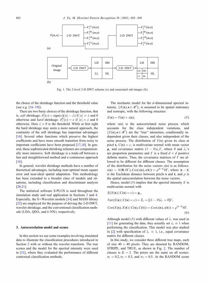
In this paper, we adopt the two-dimensional discretewavelet transform (2-D DWT) due to its fast computationalalgorithm for both decomposition and reconstruction ofthe image and also the discrete nature of the image pixels.The discrete wavelet transform results from multiresolutionanalysis [13], which involves decomposition of an image infrequency channels of constant bandwidth on a logarithmicscale. It has advantages such as similarity of data structurewith respect to the resolution (i.e., the higher resolutionimage includes the lower resolution images) and availabledecomposition at any level. These in turn can bene�t es-pecially to remotely sensed data analysis where one maywish to see macroscopic characteristics of the scene at �rststage using a low resolution level and then analyse an areaof interest in detail using an appropriate higher resolutionlevel [10].

The 2-D wavelet family has one father wavelet function and three mother wavelet functions�v,�h, and�d. Theycan be constructed by taking tensor product of 1-D wavelets.Roughly speaking, captures the smooth part, and �v, �h,and �d captures the vertical detail, the horizontal detail, andthe diagonal detail, respectively.

The 2-D wavelet approximation (at level J ) of a 2-Dfunction F(x; y) is a linear combination of 2-D wavelets atdi4erent scales and locations:

F(x; y) ≈∑k

sJ;k J;k(x; y) +J∑j=1

∑k

dvj;k�vj;k(x; y)

+J∑j=1

∑k

dhj;k�hj;k(x; y) +

J∑j=1

∑k

ddj;k�dj;k(x; y);

(3)

where k=(k1; k2)∈Z2, and ( J;k(x; y); �vj;k(x; y); �h

j;k(x; y);�d

j;k(x; y)) are the orthonormal basis functions generatedfrom the father and mother wavelets by scaling and trans-lation, and the coeNcients, the s and d’s, are the innerproducts of F and the corresponding basis functions. Inthis way, F(x; y) is decomposed into a sum of coarse res-olution (level J ) smooth coeNcients and sums of �ne tocoarse resolution (levels 1 to J ) detail coeNcients (vertical,horizontal, and diagonal).

When an M × N discrete image F(m; n) is observed,that is, the 2-D function F(x; y) is sampled, the 2-D DWTcomputes the coeNcients of the 2-D wavelet series ap-proximation (3) for it. It maps the image F(m; n) to anM × N matrix of wavelet coeNcients. For computer im-

plementation, the dimensions M and N are desirable tobe the power of 2. In S+Wavelets [14], the 2-D DWT isimplemented by using the Mallat’s [13] fast 2-D pyramidalgorithm. It consists of �ltering and down-sampling us-ing low- and high-pass �lters L and H , �rst horizontally(by rows) and then vertically (by columns). So, apply-ing the 2-D DWT to the original image F(m; n) once,we get four lower resolution sub-images consisting ofwavelet coeNcients: FLL

1 (m; n); FLH1 (m; n); FHL

1 (m; n), andFHH

1 (m; n), for m = 1; : : : ; M=2; n = 1; : : : ; N=2. The sec-ond time transform is just to split FLL

1 (m; n) in the sameway, which produces the decomposition at the secondlevel: FLL

2 (m; n); FLH2 (m; n); FHL

2 (m; n), and FHH2 (m; n), for

m= 1; : : : ; M=22; n= 1; : : : ; N=22. General expression for thehigher levels can easily be derived. Fig. 1 shows the schemafor a two-level decomposition yielding seven sub-images.

Since the wavelet coeNcients at di4erent levels and indi4erent sub-images represent the characteristics of the pix-els in the original image and also contain information onneighbouring pixels, they are used to construct the featurevector in our classi�cation task as follows:

x = (x1; : : : ; xd)T; (4)

where d denotes the dimension of the vector and the com-ponent xk ; k = 1; : : : ; d is the pixel value of a sub-image inthe wavelet transform (i.e., the corresponding wavelet coef-�cient). Thus d=1 if only the pixel value in the original im-age (i.e. the observed one-dimensional spectral signature) isused; d=4 if the wavelet transform is applied to the originalimage once; and d = 7 if the wavelet transform is appliedtwice, and so on. Thus, the dimension of the vector increaseswith the number of wavelet transform execution. Note thatthe pixels in the sub-images with lower resolution are en-larged to match pixels with the highest resolution. It is alsoworth noting that a repeated wavelet transform to a speci�cimage may serve to classi�cation of targets eNciently sincethe wavelet coeNcients account for the neighbouring pixelinformation, and consequently it becomes an advantage overthe contextual method which requires extensive computa-tion time on the correlation between adjacent pixels.

For multispectral images with m correlated bands, thewavelet transform is applied to each band separately andthe corresponding feature vector can be obtained as above.By merging these m feature vectors in to one results in the�nal feature vector of length m times larger than that forimages with single band. For example, if the number ofwavelet transform execution is 3, then the feature vector ofa two-bands image will be of length twenty.

The wavelet transform has also been used to achieve im-age compression and noise removal, where the eNciency ofthe representation is important for the clarity of the analysis.The technique is based on the principle of wavelet shrink-age [15], which refers to taking the wavelet transform ofthe image, removing noise by shrinking wavelet coeNcientstowards zero, and inverting the thresholded wavelet trans-form coeNcients. Much study has been made concerning


F(m,n) 2-D DWT

F LL1 (m,n)

F LH1 (m,n)

F HL1 (m,n)

F LL1 (m,n)

(m,n)

(m,n)

(m,n)

(m,n)

2-D DWT

F LL2

F LH2

F HL2

F LL2

image

Original2-D DWT

HHLH

HLLL

2-D DWT

HHLH

HLHHLH

HLLL

(a)

(b)

Fig. 1. The 2-level 2-D DWT schema (a) and associated sub-images (b).

the choice of the shrinkage function and the threshold value(see e.g. [16–19]).

There are two basic choices of the shrinkage function, thatis, soft shrinkage: �S�(x) = sign(x)(|x| − �) if |x|¿� and 0otherwise and hard shrinkage: �H� (x) = x if |x|¿� and 0otherwise. Here �¿ 0 is the threshold. While at �rst sightthe hard shrinkage may seem a more natural approach, thecontinuity of the soft shrinkage has important advantages[16]. Several other functions which preserve the highestcoeNcients and have more smooth transition from noisy toimportant coeNcients have been proposed [17,18]. In gen-eral, these sophisticated shrinking schemes are computation-ally more intensive. Soft shrinkage is a trade-o4 between afast and straightforward method and a continuous approach[16].

In general, wavelet shrinkage methods have a number oftheoretical advantages, including near-optimal mean squareerror and near-ideal spatial adaptation. This methodologyhas been extended to a broader class of models and sit-uations, including classi�cation and discriminant analysis[20,21].

The statistical software S-PLUS is used throughout thesimulation study and real application in Sections 3 and 4.Especially, the S+Wavelets module [14] and MASS library[22] are employed for the purpose of driving the 2-D DWT,wavelet shrinkage, and the conventional classi�cation meth-ods (LDA, QDA, and k-NN), respectively.

3. Autocorrelation model and scenes

In this section we use some examples involving simulateddata to illustrate the classi�cation procedures introduced inSection 2 with or without the wavelet transform. The truescenes and the model for the spectral intensity were usedin [11], where they evaluated the performance of di4erentcontextual classi�cation methods.

The stochastic model for the d-dimensional spectral in-tensity, {X (s); s∈R2}, is assumed to be spatial stationaryand isotropic, with the following structure:

X (s) = Y (s) + "(s); (5)

where "(s) is the autocorrelated noise process whichaccounts for the class independent variations, and{Y (s); s∈R2} are the “true” intensities, conditionally in-dependent given their classes, and also independent of thenoise process. The distribution of Y (s) given its class atpixel s, C(s) = c, is multivariate normal with mean vector�c and covariance matrix (1 − $)�c%, where $ and �c’sare proportion parameters and % is a �xed d × d positivede�nite matrix. Thus, the covariance matrices of Y are al-lowed to be di4erent for di4erent classes. The assumptionof the distribution for the noise vectors "(s) is as follows:"(s) ∼ N (0; $%); Cov("(s); "(t)) = '|s−t|$%, where |s − t|is the Euclidean distance between pixels s and t, and ' isthe spatial autocorrelation between the noise vectors.

Hence, model (5) implies that the spectral intensity X ismultivariate normal with

E(X (s) |C(s) = c) = �c;

Var(X (s) |C(s) = c) = c = [(1 − $)�c + $]%;

Cov(X (s); X (t) |C(s); C(t)) = Cov("(s); "(t)) = '|s−t|$%:(6)

Although model (5) with di4erent values of �c was used in[11] for generating the data, they actually set �c ≡ 1 whenperforming the classi�cation. This model was also studiedin [2] with speci�cation of �c ≡ 1, i.e., equal covariancematrix for di4erent classes.

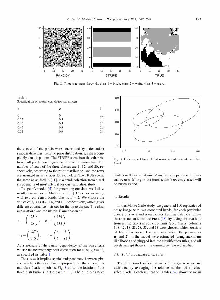
In this study, we consider three di4erent true maps, eachof size 40 × 40 pixels. They are denoted by RANDOM,STRIPE, and TRUE, as shown in Fig. 2. The number ofclasses is K = 3. The priors are the same on all scenes:�1 = 0:2; �2 = 0:3; and �3 = 0:5. At the RANDOM scene


0 10 20 30 40

RANDOM

0

10

20

30

40

0 10 20 30 40

STRIPE

0

10

20

30

40

0

10

20

30

40

0 10 20 30 40

TRUE

Fig. 2. Three true maps. Legends: class 1 = black; class 2 = white, class 3 = grey.

Table 1Speci�cation of spatial correlation parameters

, ' $

0 0 0.50.25 0.5 0.50.40 0.5 0.80.45 0.9 0.50.72 0.9 0.8

the classes of the pixels were determined by independentrandom drawings from the prior distribution, giving a com-pletely chaotic pattern. The STRIPE scene is at the other ex-treme: all pixels from a given row have the same class. Thenumber of rows of the three classes are 8, 12, and 20, re-spectively, according to the prior distribution, and the rowsare arranged in two stripes for each class. The TRUE scene,the same as studied in [11], is a small selection from a realscene and is of most interest for our simulation study.

To specify model (5) for generating our data, we followmostly the values in Mohn et al. [11]. Consider an imagewith two correlated bands, that is, d = 2. We choose thevalues of �c’s as 0.4, 1.4, and 1.0, respectively, which givesdi4erent covariance matrices for the three classes. The classexpectations and the matrix % are chosen as

�1 =

(125

128

); �2 =

(130

135

);

�3 =

(127

110

); % =

(4 8

8 81

):

As a measure of the spatial dependency of the noise termwe use the nearest neighbour correlation for class 3, ,='$,as speci�ed in Table 1.

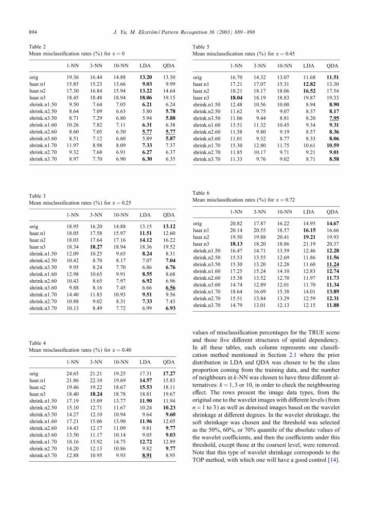
Thus, , = 0 implies spatial independency between pix-els, which is the case most appropriate for the noncontex-tual classi�cation methods. Fig. 3 shows the location of thethree distributions in the case , = 0. The ellipsoids have

120

160

140

120

100

80

125 130 135

Fig. 3. Class expectations ±2 standard deviation contours. Case, = 0.

centers in the expectations. Many of those pixels with spec-tral vectors falling in the intersection between classes willbe misclassi�ed.

4. Results

In this Monte Carlo study, we generated 100 replicates ofnoisy image with two correlated bands, for each particularchoice of scene and ,-value. For training data, we followthe approach of Klein and Press [23], by taking observationsfrom all the pixels in some columns. Speci�cally, columns3, 8, 13, 18, 23, 28, 33, and 38 were chosen, which consistsof 1/5 of the scene. For each replication, the parameters�c and c in the model were estimated (using maximumlikelihood) and plugged into the classi�cation rules, and allpixels, except those in the training set, were classi�ed.

4.1. Total misclassi7cation rates

The total misclassi�cation rates for a given scene areestimated by averaging the relative number of misclas-si�ed pixels in each replication. Tables 2–6 show the mean


Table 2Mean misclassi�cation rates (%) for , = 0

1-NN 3-NN 10-NN LDA QDA

orig 19.36 16.44 14.88 13.20 13.30haar.n1 15.85 15.23 13.66 9.03 9.99haar.n2 17.30 16.84 15.94 13.22 14.64haar.n3 18.45 18.48 18.94 18.06 19.15shrink.n1.50 9.50 7.64 7.05 6.21 6.24shrink.n2.50 8.64 7.09 6.63 5.80 5.78shrink.n3.50 8.71 7.29 6.80 5.94 5.88shrink.n1.60 10.26 7.82 7.11 6.31 6.38shrink.n2.60 8.60 7.05 6.50 5.77 5.77shrink.n3.60 8.51 7.12 6.60 5.89 5.87shrink.n1.70 11.97 8.98 8.09 7.33 7.37shrink.n2.70 9.32 7.68 6.91 6.27 6.37shrink.n3.70 8.97 7.70 6.90 6.30 6.35

Table 3Mean misclassi�cation rates (%) for , = 0:25












values of misclassi�cation percentages for the TRUE sceneand those �ve di4erent structures of spatial dependency.In all these tables, each column represents one classi�-cation method mentioned in Section 2.1 where the priordistribution in LDA and QDA was chosen to be the classproportion coming from the training data, and the numberof neighbours in k-NN was chosen to have three di4erent al-ternatives: k=1; 3 or 10, in order to check the neighbouringe4ect. The rows present the image data types, from theoriginal one to the wavelet images with di4erent levels (fromn= 1 to 3) as well as denoised images based on the waveletshrinkage at di4erent degrees. In the wavelet shrinkage, thesoft shrinkage was chosen and the threshold was selectedas the 50%, 60%, or 70% quantile of the absolute values ofthe wavelet coeNcients, and then the coeNcients under thisthreshold, except those at the coarsest level, were removed.Note that this type of wavelet shrinkage corresponds to theTOP method, with which one will have a good control [14].


Table 7Mean misclassi�cation rates (%) for STRIPE: the lowest for each,-value

, = 0 , = 0:25 , = 0:40 , = 0:45 , = 0:72

orig 13.03a 12.98a 17.16a 11.99a 15.46a

haar.n1 0.66b 3.17b 6.59b 4.68b 8.29a

haar.n2 7.86c 8.59c 9.60c 9.26c 10.79c

haar.n3 19.79c 17.66c 17.34c 17.95c 17.98c

shrink.n1.85 0.53a 2.91b 6.19a 4.33a 8.10a

shrink.n2.85 0.27a 1.21a 2.76c 2.58c 4.69c

shrink.n3.85 0.34a 1.00a 2.64c 2.59c 4.82c

shrink.n1.90 0.58a 2.91b 6.19a 4.33a 8.10a

shrink.n2.90 0.20c 1.07c 2.42c 1.89c 3.44c

shrink.n3.90 0.19a 0.78c 2.05c 1.84c 3.48c

shrink.n1.95 0.58a 2.91b 6.19a 4.33a 8.10a

shrink.n2.95 10.00a 10.16b 10.91b 11.61d 12.46c

shrink.n3.95 0.15c 0.65c 1.57c 1.23c 1.87c

aQDA.bLDA.c1-NN.d3-NN.

The wavelet function in the 2D-DWT was chosen to be thehaar wavelet because of the simple class structure of thetrue map. Thus, as an example, “shrink.n3.60” stands forthe reconstructed image by using 2D-DWT up to level 3 andthen shrinking the wavelet coeNcients with the thresholdequal to the 60% quantile. This notation for the row nameis also valid for Table 7, though the quantile level was dif-ferent there. The best results among classi�cation methodsfor each image data type (row wise) are indicated with boldface, and the total best in every table is even underlined.

What we can observe and then conclude from Tables 2–6is as follows:

• Classi�cation by using the wavelet shrinkage results inmuch lower mean classi�cation error than that workingdirectly on the original image data (the reduction can beup to 56%), and level 3 always performed better than thelower levels, except for the case when , = 0. Therefore,the wavelet transform should be executed at least twicein wavelet shrinkage.

• Classi�cation based on wavelet sub-images gives usslightly better results only at level 1 and for small,-values than working directly on the original imagedata. This is somewhat unexpected, by considering ourprevious study [24] where the classi�cation based onwavelet sub-images was very convincing. One probablereason is that the underlying true scene there was moresimple and regular, which is more comparable to theSTRIPE scene in this study.

• In general, the mean misclassi�cation rate increases as thespatial dependency between pixels strengthens. There areexceptions, however, in particular when ,= 0:40. This isprobably caused by the fact that the empirical variationin this case is clearly higher than the theoretical one.

• QDA and LDA work better than the k-NN classi�er, es-pecially in the case when k = 1. This is quite naturalbecause our model is multivariate normal which �ts thebasic requirements in LDA and QDA.

• The best result for each dependency case (i.e. the under-lined number in each table) appears where the shrinkagemethod is used and the 2D-DWT is applied three times(i.e. up to level 3), except the independent case (, = 0)where the best result is obtained at level 2.

• The threshold setting in the range of 50–70% in waveletshrinkage does not play an important role in changing themisclassi�cation rate. As we also tested di4erent thresholdlevels outside of the above range, a general impression hasbeen that for this kind of scenes the threshold should beset neither too high nor too low. The results can be muchworse if the threshold is poorly chosen. Higher and lowerthresholds are more suitable to those extreme scenes suchas STRIPE and RANDOM, respectively.

Note that only the mean values are reported in these tablesthough the corresponding standard deviations were also cal-culated. The reason was that they performed similarly withrespect to the mean values and no special outliers could beobserved. The coeNcient of variation is within the range 4.3–14.5%, 5.2–17.5%, 5.6–15.9%, 5.6–35.6% and 5.1–34.7%for , = 0, 0.25, 0.40, 0.45 and 0.72, respectively. It shouldbe noticed that the coeNcient of variation is higher for thestronger spatial correlation (' = 0:9).

For the RANDOM and STRIPE scenes, the same typeof simulation study as for the TRUE has been carried out.On the RANDOM scene, where there is no structure at all,there is generally no gain in using the wavelet methods.Using QDA on the original image data performed best forall , cases, where the misclassi�cation rates vary between11.92% and 17.68%.

On the STRIPE scene, which represents the other extreme,the results are contrary. By using the wavelet methods themean misclassi�cation rates could be reduced drastically,except one case with “haar.n3”. We summarize the corre-sponding �ve tables as on the TRUE scene into one tablefor the STRIPE scene, shown in Table 7, where the best re-sult for each ,-value is presented and the classi�cation rulesused are indicated with legends. The 1-NN classi�er basedon wavelet shrinkage with threshold 95% at level 3 is a clearwinner in all cases of spatial dependency, with a reduction(from only using the original image data) of a factor from8 when , = 0:72 up to 87 when , = 0!

It is interesting to observe that, in the case of STRIPE, thethreshold setting (from 85% to 95%) in wavelet shrinkagedoes make sense for reducing the misclassi�cation rate. Oneneeds to use only 5% of the wavelet coeNcients for obtaininga high classi�cation precision. There is one exception wherethe wavelet shrinkage with threshold 0.95 at level 2 seemsto work not so well.

It is also worth noticing that for the STRIPE scene,in general, the mean misclassi�cation rate increases as the


0 10 20 30 40

0 10 20 30 40

0 10 20 30 40 0 10 20 30 40

0 10 20 30 40

0 10 20 30 40

0

10

20

30

40

0

10

20

30

40

0

10

20

30

40

0

10

20

30

40

0

10

20

30

40

0

10

20

30

40

(a)

(c)

(e) (f)

(d)

(b)

Fig. 4. The average rates of misclassi�cation per pixel from the best classi�cation results for TRUE with di4erent ,-values: (a) QDA usingwavelet shrinkage at level 2 with threshold 0.60 for , = 0; (b) QDA using wavelet shrinkage at level 3 with threshold 0.60 for , = 0:25;(c) LDA using wavelet shrinkage at level 3 with threshold 0.70 for , = 0:40; (d) QDA using wavelet shrinkage at level 3 with threshold0.50 for , = 0:45; (e) QDA using wavelet shrinkage at level 3 with threshold 0.50 for , = 0:72; and for STRIPE with , = 0:72: (f) 1-NNusing wavelet shrinkage at level 3 with threshold 0.95.

spatial dependency of the noise term increases, and the rel-ative increase is also faster than that in the case of TRUE.Here again the case when , = 0:40 is an exception due tothe same reason as we explained before in this subsection.

4.2. Location of misclassi7ed pixels

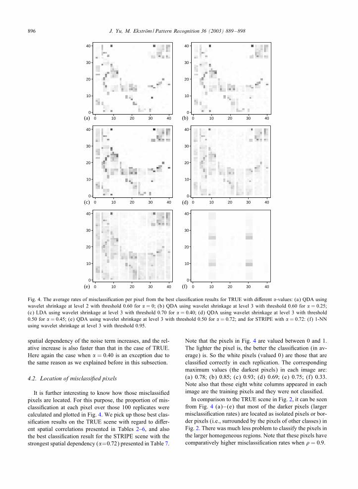
It is further interesting to know how those misclassi�edpixels are located. For this purpose, the proportion of mis-classi�cation at each pixel over those 100 replicates werecalculated and plotted in Fig. 4. We pick up those best clas-si�cation results on the TRUE scene with regard to di4er-ent spatial correlations presented in Tables 2–6, and alsothe best classi�cation result for the STRIPE scene with thestrongest spatial dependency (,=0:72) presented in Table 7.

Note that the pixels in Fig. 4 are valued between 0 and 1.The lighter the pixel is, the better the classi�cation (in av-erage) is. So the white pixels (valued 0) are those that areclassi�ed correctly in each replication. The correspondingmaximum values (the darkest pixels) in each image are:(a) 0.78; (b) 0.85; (c) 0.93; (d) 0.69; (e) 0.75; (f) 0.33.Note also that those eight white columns appeared in eachimage are the training pixels and they were not classi�ed.

In comparison to the TRUE scene in Fig. 2, it can be seenfrom Fig. 4 (a)–(e) that most of the darker pixels (largermisclassi�cation rates) are located as isolated pixels or bor-der pixels (i.e., surrounded by the pixels of other classes) inFig. 2. There was much less problem to classify the pixels inthe larger homogeneous regions. Note that these pixels havecomparatively higher misclassi�cation rates when ' = 0:9.


5. Discussion and conclusion

The discrete wavelet transform provides multiresolutionrepresentation of an image and captures the di4erent de-tails on texture as well as information on neighbouring pix-els. This information is contained in the wavelet coeNcientswhich are in turn assigned as the components of the featurevector of a pixel. By using wavelet shrinkage we can e4ec-tively remove the Gaussian noise from images and there-fore improve the classi�cation results. Our simulation studyshowed that no matter which type of spatial correlation be-tween pixels the image has and which kind of conventionalclassi�cation method one uses, the classi�cation by using thewavelet transform (specially the wavelet shrinkage) yieldsa much lower classi�cation error than that working directlyon the original image data, as soon as we have a class im-age with some structure in it. The study also indicates thatweakening the spatial dependency in the data (by decreas-ing ' while keeping $ �xed) reduces the misclassi�cationrate when the wavelet method is employed.

Note that results can be even better by optimising waveletshrinkage via varying di4erent choices of thresholds andwavelet functions. Concerning the threshold assessment, ingeneral, a threshold is a trade-o4 between closeness of �tand smoothness. A small threshold yields a result close tothe input and a larger one produces an output with a simpleand smooth representation in the chosen basis. Paying toomuch attention to smoothness however destroys some of thesignal singularity, in image processing it may cause blurand artifacts [16]. This has been reKected in our simulationresults: the threshold level should be set quite high when theoriginal image is very regular and simple structured such asthe STRIPE scene, while it should be very low when theoriginal image is of chaotic pattern such as the RANDOMscene. Otherwise, the threshold should be of moderate sizeas shown in the case of TRUE scene. In real application,however, the situation is more complicated and the selectionof threshold and wavelet functions will not be an easy task.Often one has no replicates of the image under investigationso that the performance of di4erent methods can not beevaluated as in our Monte Carlo study. Alternatively, we canmake our selection through estimating the misclassi�cationrate by using cross-validation or bootstrap methods and theground reference data. Examples can be found in [24,25].

Compared to contextual classi�cation methods which re-quire extensive computation time on correlation between ad-jacent pixels, the discrete wavelet transform provides a veryeNcient tool (due to the fast pyramid algorithm) for appli-cations using satellite images with a large amount of pixels.It should be mentioned that there was an idea in this study tocompare the contextual classi�cation methods such as thosestudied in Mohn et al. [11] with the wavelet-based classi�-cation methods. But the comparison could not be conducteddue to the limitations of the contextual methods. Speci�-cally, the spatial correlations ' and $ could not be properlyestimated no matter what estimation methods including that

used in [11]. We found that the estimates were very unsta-ble, often giving values outside the interval [0; 1].

One more disadvantage of the contextual methods is therequirement on the training data that is of the form of (homo-geneous) crossings or the like. This is not easily accessiblein practice, often due to the limitation of resources (suchas �nance, time, well-trained surveyors) and also the inven-tory season, based on our experiences in real application oflarge-scale inventory.

There are possibilities of further development associatedwith the use of the wavelet transform in image classi�ca-tion problem. For example, how to further utilise the inher-ent properties of wavelet coeNcients such as dependencywithin and between the resolution levels (an application ofhidden Markov chain to this problem has been investigatedfor one-dimensional signal analysis [26]).

The present study has convinced us that the waveletmethod attend to be useful in the subject of statistical clas-si�cation of remotely sensed imagery. An evaluation of theperformance on Landsat TM image with a single band wasmade in [24], which showed that using the k-NN classi�ertogether with the wavelet transform outperformed thoseonly applied to the original image. We believe that similarperformance can be obtained when applying to Landsat TMimage with two or more correlated bands, and this will bedone in a separate paper.

Acknowledgements

We are grateful for the valuable comments provided bythe referee. This work is a part of the Swedish researchprogramme “Remote Sensing for the Environment”, RESE(home page http://www.lantmateriet.se/rese/), �nanced bythe Swedish Foundation for Strategic Environmental Re-search, MISTRA. The authors would also like to thank Prof.Bo Ranneby and Dr. Mats Nilsson for helpful commentsand discussion.

References

[1] F.J. Cortijo, N. Perez De La Blanca, Improving classicalcontextual classi�cations, Int. J. Remote Sensing 19 (8)(1998) 1591–1613.

[2] A.M. Flygare, Classi�cation of remotely sensed data utilisingthe autocorrelation between spatio-temporal neighbours,Ph.D. Thesis, Department of Mathematical Statistics, UmeUaUniversity, 1997.

[3] K.M.S. Sharma, A. Sarkar, A modi�ed contextual classi-�cation technique for remote sensing data, PhotogrammetricEng. Remote Sensing 64 (4) (1998) 273–280.

[4] T. Watanabe, H. Suzuki, S. Tanba, R. Yokoyama, Improvedcontextual classi�ers of multispectral image data, IEICETrans. Fund. E77-A (9) (1994) 1445–1450.

http://www.lantmateriet.se/rese/


[5] A. Aldroubi, M. Unser, Wavelets in Medicine and Biology,CRC Press, Boca Raton, FL, 1996.

[6] A. Antoniadis, G. Oppenheim, Wavelet and Statistics,Springer, New York, 1995.

[7] J.S. Byrnes, J.L. Byrnes, K.A. Hargreaves, K. Berry, Waveletsand Their Applications, Kluwer Academic Publishers,Dordrecht, 1994.

[8] K.J. Jones, 3-D wavelet image processing for spatial andspectral resolution of landsat images, SPIE Proc. 3391 (1998)218–225.

[9] H.H. Szu, J.L. Moigne, N.S. Netanyahu, C.C. Hsu, Integrationof local texture information in the automatic classi�cation ofLandsat images, SPIE Proc. 3078 (1997) 116–127.

[10] Y. Yamaguchi, T. Nagai, H. Yamada, JERS-1 SAR imageanalysis by wavelet transform, IEICE Trans. Commun. E78-B(12) (1995) 1617–1621.

[11] E. Mohn, N.L. Hjort, G.O. Storvik, A simulation study ofsome contextual classi�cation methods for remotely senseddata, IEEE Trans. Geosci. Remote Sensing GE-25 (6) (1987)796–804.

[12] B.D. Ripley, Pattern Recognition and Neural Networks,Cambridge University Press, Cambridge, UK, 1996.

[13] S. Mallat, The theory for multiresolution signal decom-position: the wavelet representation, IEEE Trans. Pattern Anal.Mach. Intell. 11 (7) (1989) 654–693.

[14] A. Bruce, H.Y. Gao, Applied Wavelet Analysis with S-PLUS,Springer, New York, 1996.

[15] D.L. Donoho, I.M. Johnstone, G. Kerkyacharian, D. Picard,Wavelet shrinkage: asymptopia?, J. R. Stat. Soc. Ser. B 57(1995) 301–369.

[16] M. Jansen, Noise Reduction by Wavelet Thresholding,Springer, New York, 2001.

[17] H.Y. Gao, A.G. Bruce, WaveShrink with �rm shrinkage, Stat.Sinica 7 (4) (1997) 855–874.

[18] H.Y. Gao, Wavelet shrinkage denoising using thenon-negative garrots, J. Comput. Graph. Stat. 7 (4) (1998)469–488.

[19] D.L. Donoho, I.M. Johnstone, Ideal spatial adaptation bywavelet shrinkage, Biometrika 81 (1994) 425–455.

[20] J.B. Buckheit, D.L. Donoho, Improved linear discriminantanalysis using time-frequency dictionaries, Technical Report,Stanford University, 1995.

[21] N. Saito, R. Coifman, Local discriminant bases, SPIE Proc.—Wavelet Appl. 2303 (1994) 2–14.

[22] W.N. Venables, B.D. Ripley, Modern Applied Statistics withS-PLUS, 2nd Edition, Springer, New York, 1997.

[23] R. Klein, S.J. Press, Contextual Bayesian classi�cation ofremotely sensed data, Commun. Stat.—Theory Methods 18(9) (1989) 3177–3202.

[24] J. Yu, M. Ekstr(om, M. Nilsson, Image classi�cation usingwavelets with application to forestry, Proceedings of theFourth International Conference on Methodological Issues inONcial Statistics, Stockholm, 2000.

[25] B.M. Steele, J.C. Winne, R.L. Redmond, Estimation andmapping of misclassi�cation probabilities for thematicland cover maps, Remote Sensing Environ. 66 (1998)192–202.

[26] M.S. Crouse, R.D. Nowak, K. Mhirsi, R.G. Baraniuk,Wavelet-domain hidden Markov models for signal detectionand classi�cation, SPIE Proc. 3162 (1997) 36–47.

About the Author—JUN YU received his B.S. degree in Mathematics from Hangzhou University, Hangzhou, China, in 1982, and Ph.D.degree in Mathematical Statistics from UmeUa University, Sweden, in 1994.

From 1994 to 1998, he was a senior lecturer and research associate in the Department of Mathematical Statistics, UmeUa University,Sweden. Since January 1999, he is an associate professor in the Centre of Biostochastics, Department of Forest Resource Management andGeomatics at the Swedish University of Agricultural Sciences, UmeUa, Sweden. His current research interests include statistical classi�cationof remotely sensed imagery, wavelet theory applied to statistical problems, pattern recognition, myoeletric signal analysis, application ofthe methods of spatial statistics to forest and environmental data.

He is a member of the Bernoulli Society for Mathematical Statistics and Probability, the International Biometric Society, the InternationalChinese Statistician Association and the Swedish Statistician Association.

About the Author—MAGNUS EKSTR (OM received his MS and PhD degrees in Mathematical Statistics from UmeUa University, Sweden,in 1992 and 1997, respectively. Since 1997 he is an assistant professor in the Centre of Biostochastics, Department of Forest ResourceManagement and Geomatics at the Swedish University of Agricultural Sciences, UmeUa, Sweden. From January to June 1998, he was avisiting assistant professor at University of California, Santa Barbara, USA. His research interests include estimation theory, resamplingtechniques, spatial statistics, and classi�cation theory.

Documents

Multispectral image classification using wavelets: a simulation study