Multistage K-Means Clustering for Scenario Tree Construction

INFORMATICA, 2010, Vol. 21, No. 1, 123–138 123© 2010 Institute of Mathematics and Informatics, Vilnius

Multistage K-Means Clusteringfor Scenario Tree Construction

Kristina ŠUTIENE, Dalius MAKACKAS, Henrikas PRANEVICIUSDepartment of Business Informatics, Kaunas University of TechnologyStudent ↪u 56-301, LT-51424 Kaunas, Lithuaniae-mail: [email protected]

Received: January 2008; accepted: October 2009

Abstract. In stochastic programming and decision analysis, an important issue consists in the ap-proximate representation of the multidimensional stochastic underlying process in the form of sce-nario tree. This paper presents the approach to generate the multistage multidimensional scenariotree out of a set of scenario fans. For this purpose, the multistage K-means clustering algorithm isdeveloped. The presented scenario tree generation algorithm is motivated by the stability results foroptimal values of a multistage stochastic program. The time complexity of developed multistageK-means clustering algorithm is proved to be linear in regard to the number of scenarios in the fan.The algorithm to determine the branches with nonduplicate information in the multistage scenariotree is also presented as an intermediate result of research.

Keywords: scenario generation, scenario tree, multistage K-means clustering, time complexity.

1. Introduction and Problem Statement

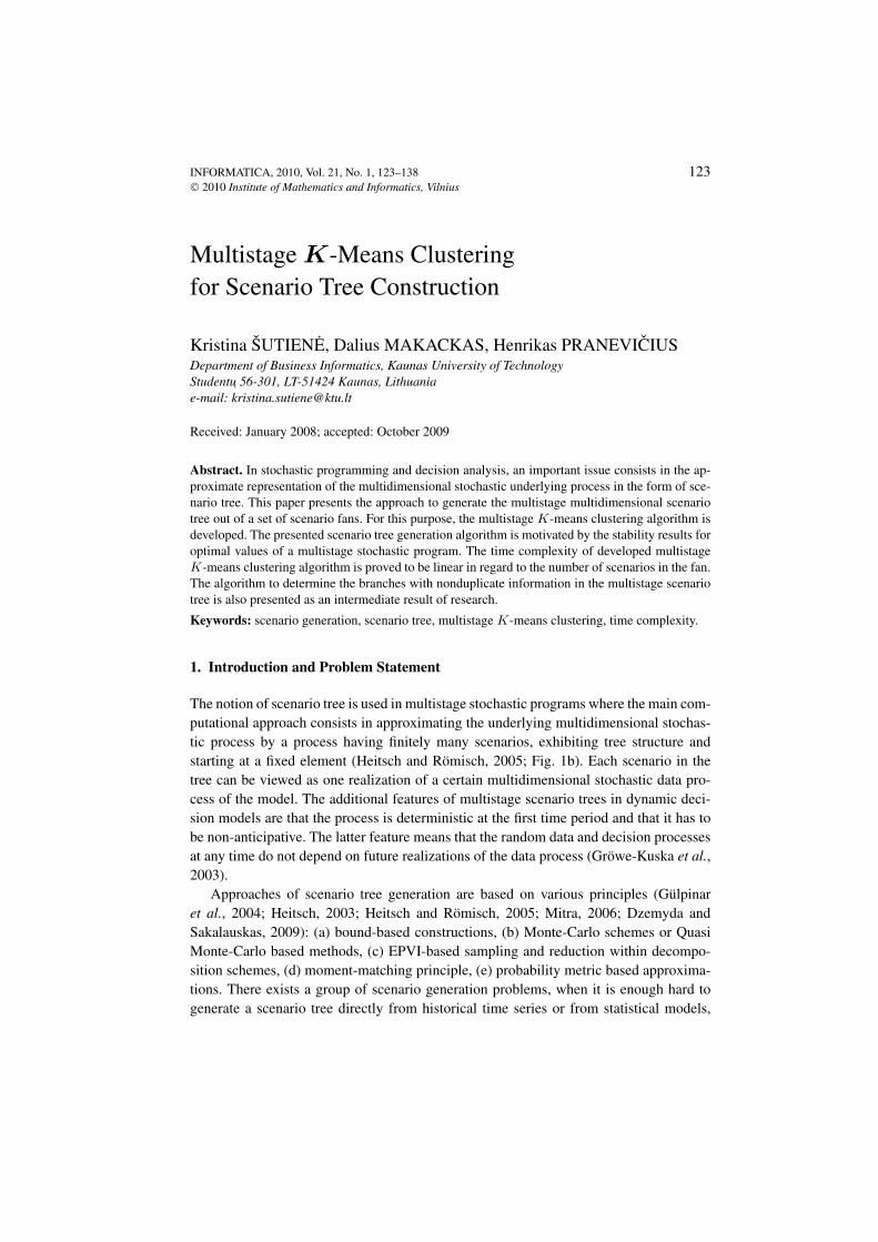
The notion of scenario tree is used in multistage stochastic programs where the main com-putational approach consists in approximating the underlying multidimensional stochas-tic process by a process having finitely many scenarios, exhibiting tree structure andstarting at a fixed element (Heitsch and Römisch, 2005; Fig. 1b). Each scenario in thetree can be viewed as one realization of a certain multidimensional stochastic data pro-cess of the model. The additional features of multistage scenario trees in dynamic deci-sion models are that the process is deterministic at the first time period and that it has tobe non-anticipative. The latter feature means that the random data and decision processesat any time do not depend on future realizations of the data process (Gröwe-Kuska et al.,2003).

Approaches of scenario tree generation are based on various principles (Gülpinaret al., 2004; Heitsch, 2003; Heitsch and Römisch, 2005; Mitra, 2006; Dzemyda andSakalauskas, 2009): (a) bound-based constructions, (b) Monte-Carlo schemes or QuasiMonte-Carlo based methods, (c) EPVI-based sampling and reduction within decompo-sition schemes, (d) moment-matching principle, (e) probability metric based approxima-tions. There exists a group of scenario generation problems, when it is enough hard togenerate a scenario tree directly from historical time series or from statistical models,

124 Šutiene et al.

Fig. 1. The usage of multistage K-means clustering method in generating the scenario tree out of scenario fan.

e.g., time series or regression models. Thus, the idea is to start with a good initial approx-imation of the underlying stochastic input process so that a fan of individual scenarios iscreated (Fig. 1a). These scenarios can be obtained by sampling or simulation techniquesbased on stochastic model. Clearly, a good approximation may involve a large number ofscenarios. Although such fan of individual scenarios represents a very specific scenariotree (2-stage problem), its structure is not appropriate for the stage-wise decision processand contains a large number of nodes (Heitsch and Römisch, 2005).

To eliminate these disadvantages, the initial scenario fan is modified by bundling sim-ilar scenarios to construct the multistage scenario tree. The researches based on suchprinciple have been published, e.g., in Gröwe-Kuska et al. (2003) a subset of the ini-tial scenario set is determined and the procedure based on a recursive reduction argu-ment using transportation metrics is presented, in Heitsch and Römisch (2005), Mölleret al. (2004) the backward and forward scenario tree generation methods based on upperbounds for two relevant ingredients of the stability estimate, namely, the probabilistic andthe filtration distance, are described.

We propose the algorithm based on method from cluster analysis to construct themultistage scenario tree by bundling similar scenarios in the scenario fan (Fig. 1). Anapproach similar to our work is introduced in the article Dupacová et al. (2002), butwithout a detailed clustering algorithm. Due to this, K-means clustering method is mod-ified to treat properly the inter-stage dependencies, and it is implemented while con-structing the multistage scenario tree from the fan of individual scenarios. The developedmethod allows to cluster similar scenarios from d scenario fans. Thus, the multistaged-dimensional scenario tree is obtained, and the method is named as multistage K-meansclustering. This paper is a continuous research of paper Pranevicius and Šutiene (2007),where the precision of approximation of scenario fans by the scenario tree is evaluated.

The other question considered in this paper is the redundancy elimination in the multi-stage scenario tree. The redundancy is identified if the scenario tree is described scenarioby scenario, i.e., one could think of the scenarios as paths from the root node to the leaves(Gassmann, 2006). Thus, scenarios may share data for several stages: information up tothe branch period is shared between a scenario and its parent scenario. It is useful forsystem comprehension to remove redundancy and to identify branches in the scenariotree with nonduplicate information (Gassmann and Kristjánsson, 2008). For this purpose,

Multistage K-Means Clustering for Scenario Tree Construction 125

the algorithm based on idea of labelling on branches is developed and described in thispaper.

The third part of the paper addresses to the question of testing the stability of proposedscenario tree generation method, according to the reference of Kaut and Wallace (2003),since the procedure of tree construction involves the randomness. It is demonstrated on acase from asset liability management, which is a problem from stochastic programming.

2. Notation for Scenarios

Scenarios are introduced as atoms of the true discrete probability distribution P or ofthat discrete probability distribution which approximates the true one. The notation forscenarios is given based on the references Domenica et al. (2007), Dupacová et al. (2000).

If a stochastic factor evolves in time, we have a stochastic process. Let assume that thestochastic process ξ = {ξt}T t

t=1 is defined on some filtered probability space (Ω, S, F , P ).The sample space Ω is defined as Ω := Ω1 × Ω2 × · · · × ΩT t , where Ωt ⊂ Rd aretaken as finite dimensional. For instance, these data may correspond to the random returnof d financial assets at different time moments t. The σ-algebra S is the set of eventswith assigned probabilities by measure P , and {Ft}T t

t=1 is a filtration on S. For scenariobased models, one assumes that the probability distribution P is discrete and concentratedon a finite number of points, say, ξs = (ξs

1, . . . , ξst , . . . , ξ

sT t), ξs

t = (ξs,1t , . . . , ξs,d

t )′,

s = 1, . . . , S. The probability of ξst is denoted as πs

t� = πs

t� (ξs

t ),∑S

s=1 πst

� = 1,

t ∈ {1, . . . , T t}. At the current time moment t0, all scenarios are known with cer-tainty. Thus, the first stage is represented by a single root node ξ0 (vector in Rd). Mov-ing to the second stage, the structure branches into individual scenarios. Such struc-ture of simulated data paths is called as scenario fan (Fig. 1a). It is represented astwo-stage problem, as all σ-fields Ft, t = 1, . . . , T t coincide. Thus, the probabilitiesπs

t� = πs

t′�

, s = 1, . . . , S, t �= t′, t, t′ > 0. The two-stage stochastic problem has thefollowing properties, as in Dupacová et al. (2000): decisions at all time instances aremade at once and no further information is expected; except for the first stage no non-anticipativity constraints appear. In general, such properties can be regarded as disadvan-tages, especially in cases, when decisions are considered to be reformulated during thehorizon. By eliminating these disadvantages, the multistage scenario tree is generated.

The multistage scenario tree (Fig. 1b) allows to reflect the inter-stage dependencyand decreases the number of nodes while comparing to the scenario fan. The time stageindex τ ∈ {1, . . . , T τ } is associated with time moments when decisions are taken.The structure of multistage scenario tree at initial time moment is described by a soleroot node ξ0 (vector in Rd) and by branching into a finite number of scenarios in ev-ery stage. The probability distribution P is concentrated on a finite number of pointsξsT τ = (ξs1

1 , . . . , ξsττ , . . . , ξsT τ

T τ ), ξsττ = (ξsτ ,1

τ , . . . , ξsτ ,dτ )′, sτ = 1, . . . , Sτ , but with

varying size of scenarios set Sτ . The probability of ξsττ is denoted as πst

t�� = πst

t�� (ξsτ

τ ).The stages are connected with possibility to take additional decisions based on newlyrevealed information. Such information can be obtained periodically (every day, week,

126 Šutiene et al.

month) or based on some events (expiration of investment portfolio duration). The dis-tinction between stages and time periods of discretization is essential, because in practicalapplication it is important that the number of time periods would be greater than the cor-responding nodes. The arcs linking nodes represent various realizations of random vari-ables. The number of branches from each node can vary depending on problem specificrequirements and not definitely constant through the tree.

3. Construction of Multistage Multidimensional Scenario Treeout of the Scenario Fans

At this moment, we concentrate on the construction of scenario trees when the underly-ing stochastic parameters have been determined and the individual scenarios are alreadygenerated. Based on scenario’s dimension, the scenario trees can be of two types:

• The multistage scenario tree, which is generated from one scenario fan (one-dimensional scenarios).

• The d-dimensional multistage scenario tree, which is generated from d scenariofans (d-dimensional scenarios).

The scenario tree is used to describe the behaviour of one uncertain factor; thed-dimensional scenario tree is used to describe the behaviour of d uncertain factors.

To bundle the individual scenarios into clusters, the clustering procedure is employed.Clustering consists in partitioning of a set of scenarios into subsets, so that the scenariosinside cluster would be more similar than outside the cluster. Since most of clusteringmethods are developed for data not varying in time, we have to make some modifi-cations in order to cluster the time dependent data, such as are scenarios. Due to this,K-means clustering method (Kaufmann and Rousseeuw, 1990; Teknomo, 2006; Krilavi-cius and Žilinskas, 2008) is modified to treat properly the inter-stage dependencies, and itis implemented while constructing the multistage scenario tree out of scenario fans. Twofactors are used to delineate the structure of scenario tree: the branching scheme and thenumber of stages. Let assume that branches Kτ are desired from each scenario tree nodeat stage τ . For example, in the case of Kτ = 2 the pessimistic and optimistic scenariosare considered. In the terminology of cluster analysis, it means that Kτ clusters have tobe formed. The following modifications for K-means method have to be done in order toconstruct the scenario tree with (τ + 1) stages:

• In the current stage, the new sub-clusters have to be formed from each clustergenerated at previous stage.

• Centroids (means) have to be computed only at stage indexed time moments, whilethe distance measure has to exploit the whole sequence of simulated d-dimensionalscenarios.

• The possibility of changing the number of clusters in every stage has to be allowed.• The probabilities of each node have to be evaluated.

After a discussion of a kind of requirements we are using, the multistage K-meansclustering problem and then the algorithm for solving it are described below.


3.1. The Multistage K-Means Clustering Problem

Given a set of d-dimensional scenarios ξs = (ξst ), where ξs

t = (ξs,jt ), s = 1, . . . , S,

t ∈ {1, . . . , T t}, j = 1, . . . , d, and the number Kτ of desired clusters at stageτ ∈ {1, . . . , T τ }, it is needed to solve κτ K-means clustering tasks in each stage τ ,where

κτ =

{ ∏τ −1j=1 Kj , τ > 1,

1, τ = 1.

The input to each of 1, . . . , κτ K-means clustering tasks is ξs ∈ Ckτ , k = 1, . . . , κτ ,

which are formed while performing usual K-means clustering algorithm. The output ofstage τ are cluster’s centroids ξk = (ξk

t ), where t = τ, k = 1, . . . ,∏τ

j=1 Kj with

assigned probabilities π��(ξk).

3.2. The Multistage K-Means Clustering Algorithm

Set the stage indexed time moments as τ ∈ {1, . . . , T τ }, then iterate the following steps:Step 1. Setting initial centroids. Let ξk = (ξk

t ), t ∈ {1, . . . , T t}, k = 1, . . . , Kτ bethe clusters’ centroids. Some method can be employed to choose the centroids’ positionsfor initial clusters, sometimes known as “seeds”. It might be chosen to be the first Kτ

scenarios or scenarios by random since the scenarios are independently generated.Step 2. Cluster assignment. Assign each scenario ξs = (ξs

t ), t ∈ {1, . . . , T t},s = 1, . . . , S to the cluster Ck = (Ck

τ ), k = 1, . . . , Kτ , such that centroid ξk = (ξkt )

is nearest to ξs = (ξst ) by the distance measure, i.e., compute the value of indicator

function:

δ(ξs, Ck

)=

{1, D

(ξs, ξk

)< D

(ξs, ξm

)for all k, m = 1, . . . , Kt, k �= m,

0, otherwise,

where D(ξs, ξk) =∑T t

t=0 ‖ξst − ξk

t ‖2 =∑T t

t=0

√∑dj=1(ξ

s,jt − ξk,j

t )2, s = 1, . . . , S,j = 1, . . . , d, k = 1, . . . , Kτ . It is possible to apply other distance metrics, such as Man-hattan distance, Maximum norm, Mahalanobis distance, in bundling similar scenarios,only some modifications have to be done in order to exploit the whole simulated datasequence.

Step 3. Centroid’s evaluation. Compute ξk = (ξkt ) as the mean of all scenarios as-

signed to cluster Ck:

ξk = E{ξs}ξs ∈Ck =1

|Ck |

S∑s=1

δ(ξs, Ck)ξs,

where |Ck | =∑S

s=1 δ(ξs, Ck) is the number of scenarios in the cluster Ck. The calcula-tion of mean can be replaced by other estimate, such as median or mode.

128 Šutiene et al.

Step 4. Repeat. Go to Step 2 until convergence. The termination criteria of conver-gence may be chosen as follows:

• Termination when convergence criteria is met, e.g., no (or very small) number ofscenarios are assigned to different clusters, squared error.

• Termination when a fixed number of iterations has been carried out (this can alsoensure stopping without convergence.

Step 5. Calculation of probabilities. Probability of ξk is equal to the sum of probabil-ities of individual scenarios ξs, belonging to the relevant cluster Ck. The probability canbe evaluated from:

π��(ξk) = |Ck |/S,

where |Ck | =∑S

s=1 δ(ξs, Ck) is the number of scenarios in the cluster Ck.Step 6. Modification. Modify ξs = (ξs

0, . . . , ξst , . . . , ξs

T t) by replacing ξst with ξk

t ifξst ∈ Ck and t = τ .

Step 7. Repeat. Go to Step 1 if the next stage index exists. The clustering proce-dure starts over for each cluster ξs ∈ Cj formed in the current stage separately, wherej = 1, . . . ,

∏τj=1 Kj .

This algorithm produces a separation of scenarios into groups. The given algorithmlets to treat properly the inter-stage dependencies, exploiting the whole sequence of simu-lated scenario path. New sub-clusters are constructed from previous generated clusters ateach defined stage, that’s why this approach is named as multistage K-means clusteringwith varying Kτ , τ ∈ {1, . . . , T τ } in every stage. The output of multistage K-meansclustering algorithm is the multistage scenario tree, which is delineated by nodes con-taining a cluster of scenarios (vectors in Rd), one of which is designated as centroidsξm = (ξm

τ ), ξmτ = (ξm,j

τ ), m = 1, . . . ,∏τ

j=1 Kj , j = 1, . . . , d, τ ∈ {1, . . . , T τ } with

assigned probabilities π��(ξm

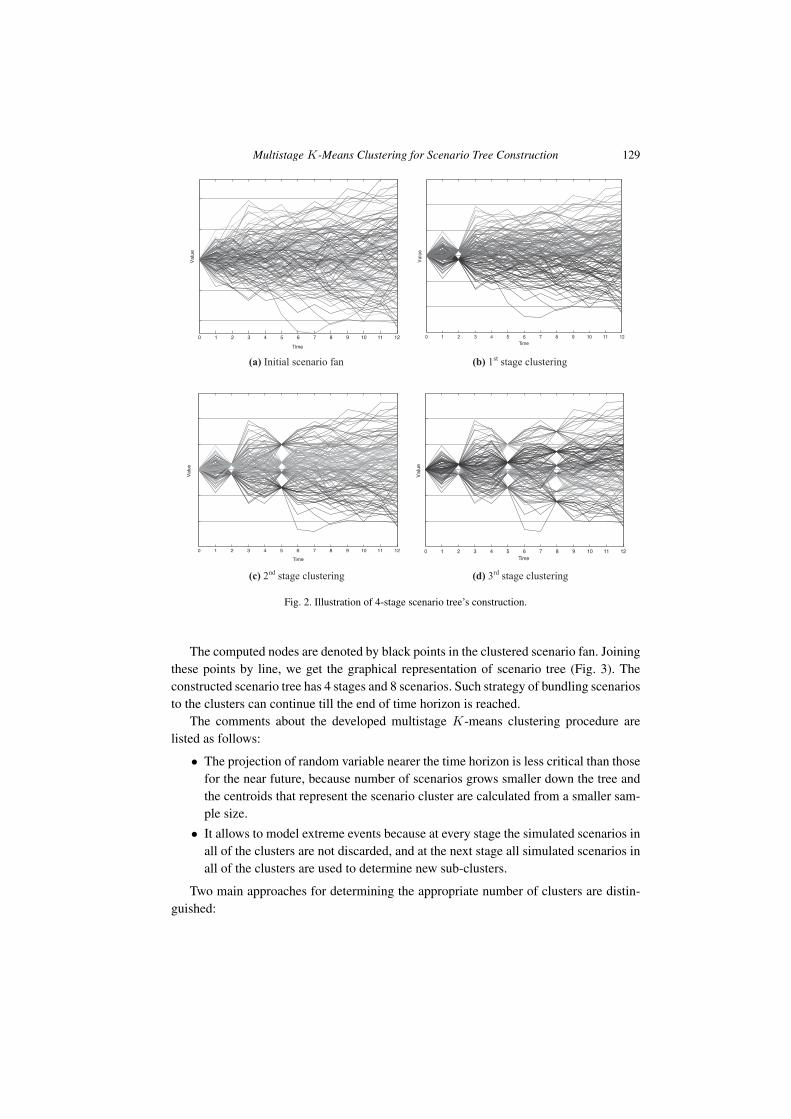
τ ) and the branching scheme Kτ .The described idea of bundling scenarios to the clusters is illustrated in Fig. 2, where

the scenario fan is chosen to consist of one-dimensional data paths for better illustrationof clustering performance. It is assumed that a set of individual scenarios for the entiretime horizon (12 time moments) is already generated (Fig. 2a). The scenario fan of 100scenarios is schematically illustrated. Let assume that we have three decision dates, i.e.,we are planning to make decisions at 2, 5 and 8 time moments. Using the given notation,we have τ = 1, 3. The strategy is to construct the scenario tree with two branches Kτ = 2per each node in every stage τ . With this initial setting, we are ready to construct the4-stage scenario tree. Thus, at the 1st decision moment (τ = 1, time = 2) two clustersare formed by the first stage of multistage clustering algorithm (Fig. 2b). The centroidof each cluster is computed, which represents the second-stage node. Next, at previousstep formed clusters are divided into two sub-clusters. It results that for the 2nd decisionmoment (τ = 2, time = 5) we have four clusters representing third-stage nodes (Fig. 2c).Finally, the result of the third-stage of K-means clustering algorithm is eight clusters,since two more sub-clusters are formed from previous clusters at the 3rd decision moment(τ = 3, time = 8; Fig. 2d).


Fig. 2. Illustration of 4-stage scenario tree’s construction.

The computed nodes are denoted by black points in the clustered scenario fan. Joiningthese points by line, we get the graphical representation of scenario tree (Fig. 3). Theconstructed scenario tree has 4 stages and 8 scenarios. Such strategy of bundling scenariosto the clusters can continue till the end of time horizon is reached.

The comments about the developed multistage K-means clustering procedure arelisted as follows:

• The projection of random variable nearer the time horizon is less critical than thosefor the near future, because number of scenarios grows smaller down the tree andthe centroids that represent the scenario cluster are calculated from a smaller sam-ple size.

• It allows to model extreme events because at every stage the simulated scenarios inall of the clusters are not discarded, and at the next stage all simulated scenarios inall of the clusters are used to determine new sub-clusters.

Two main approaches for determining the appropriate number of clusters are distin-guished:

130 Šutiene et al.

Fig. 3. Graphical representation of 4-stage scenario tree.

• Compatible cluster merging, when the clustering procedure starts with a suffi-ciently large number of clusters, and then this number is reduced by merging clus-ters that are similar (compatible) with respect to some predefined criteria (Setnes,1999).

• Usage of validity measures to assess the goodness of obtained partitions for differ-ent values of number of clusters. Different validity measures, such as Dunn’s index,Alternative Dunn’s index or Silhouette value, have been proposed in the literature,none of them is perfect by oneself (Bruna et al., 2007).

4. The Time Complexity of Multistage K-Means Algorithm

The time complexity refers to a function describing how much time it will take an algo-rithm to execute, based on the parameters of its input. An exact value of this function isusually ignored in favour of its order, expressed in O-notation.

In the case of one-dimensional scenarios, the time complexity of one-stage K-meansclustering algorithm is estimated referring to the results given in references Lin et al.(2004), Arthur and Vassilvitskii (2006). We get:

T1(S) = O(ST tKI),

where T t is the length of scenario, K is the number of clusters specified by the user,and I is the number of iterations until convergence of K-means clustering. The distancemeasure for one-dimensional scenarios is:

D(ξs, ξk) = ‖ξs − ξk ‖2 =

√√√√ T t∑t=0

(ξst − ξk

t )2, s = 1, . . . , S, k = 1, . . . , K.

Next, let evaluate the time complexity of multistage K-means clustering algorithm.


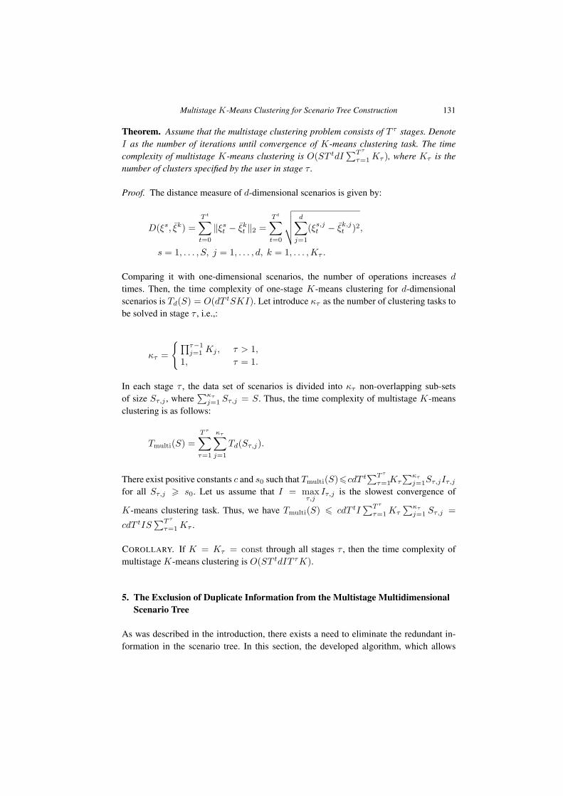
Theorem. Assume that the multistage clustering problem consists of T τ stages. DenoteI as the number of iterations until convergence of K-means clustering task. The timecomplexity of multistage K-means clustering is O(ST tdI

∑T τ

τ=1 Kτ ), where Kτ is thenumber of clusters specified by the user in stage τ .

Proof. The distance measure of d-dimensional scenarios is given by:

D(ξs, ξk) =T t∑t=0

‖ξst − ξk

t ‖2 =T t∑t=0

√√√√ d∑j=1

(ξs,jt − ξk,j

t )2,

s = 1, . . . , S, j = 1, . . . , d, k = 1, . . . , Kτ .

Comparing it with one-dimensional scenarios, the number of operations increases d

times. Then, the time complexity of one-stage K-means clustering for d-dimensionalscenarios is Td(S) = O(dT tSKI). Let introduce κτ as the number of clustering tasks tobe solved in stage τ , i.e.,:

κτ =

{ ∏τ −1j=1 Kj , τ > 1,

1, τ = 1.

In each stage τ , the data set of scenarios is divided into κτ non-overlapping sub-setsof size Sτ,j , where

∑κτ

j=1 Sτ,j = S. Thus, the time complexity of multistage K-meansclustering is as follows:

Tmulti(S) =T τ∑τ=1

κτ∑j=1

Td(Sτ,j).

There exist positive constants c and s0 such that Tmulti(S)�cdT t∑T τ

τ=1Kτ

∑κτ

j=1Sτ,jIτ,j

for all Sτ,j � s0. Let us assume that I = maxτ,j

Iτ,j is the slowest convergence of

K-means clustering task. Thus, we have Tmulti(S) � cdT tI∑T τ

τ=1 Kτ

∑κτ

j=1 Sτ,j =

cdT tIS∑T τ

τ=1 Kτ .

COROLLARY. If K = Kτ = const through all stages τ , then the time complexity ofmultistage K-means clustering is O(ST tdIT τK).

5. The Exclusion of Duplicate Information from the Multistage MultidimensionalScenario Tree

As was described in the introduction, there exists a need to eliminate the redundant in-formation in the scenario tree. In this section, the developed algorithm, which allows

132 Šutiene et al.

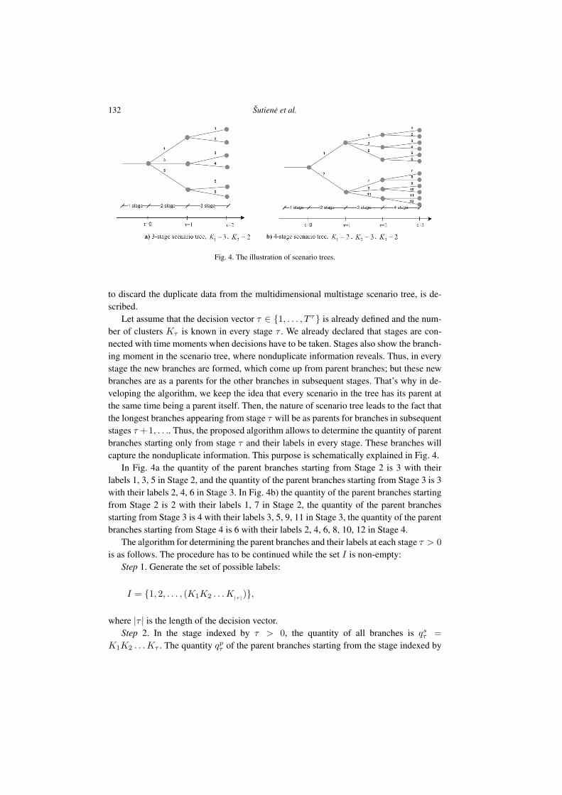
Fig. 4. The illustration of scenario trees.

to discard the duplicate data from the multidimensional multistage scenario tree, is de-scribed.

Let assume that the decision vector τ ∈ {1, . . . , T τ } is already defined and the num-ber of clusters Kτ is known in every stage τ . We already declared that stages are con-nected with time moments when decisions have to be taken. Stages also show the branch-ing moment in the scenario tree, where nonduplicate information reveals. Thus, in everystage the new branches are formed, which come up from parent branches; but these newbranches are as a parents for the other branches in subsequent stages. That’s why in de-veloping the algorithm, we keep the idea that every scenario in the tree has its parent atthe same time being a parent itself. Then, the nature of scenario tree leads to the fact thatthe longest branches appearing from stage τ will be as parents for branches in subsequentstages τ +1, . . .. Thus, the proposed algorithm allows to determine the quantity of parentbranches starting only from stage τ and their labels in every stage. These branches willcapture the nonduplicate information. This purpose is schematically explained in Fig. 4.

In Fig. 4a the quantity of the parent branches starting from Stage 2 is 3 with theirlabels 1, 3, 5 in Stage 2, and the quantity of the parent branches starting from Stage 3 is 3with their labels 2, 4, 6 in Stage 3. In Fig. 4b) the quantity of the parent branches startingfrom Stage 2 is 2 with their labels 1, 7 in Stage 2, the quantity of the parent branchesstarting from Stage 3 is 4 with their labels 3, 5, 9, 11 in Stage 3, the quantity of the parentbranches starting from Stage 4 is 6 with their labels 2, 4, 6, 8, 10, 12 in Stage 4.

The algorithm for determining the parent branches and their labels at each stage τ > 0is as follows. The procedure has to be continued while the set I is non-empty:

Step 1. Generate the set of possible labels:

I = {1, 2, . . . , (K1K2 . . . K|τ | )},

where |τ | is the length of the decision vector.Step 2. In the stage indexed by τ > 0, the quantity of all branches is qs

τ =K1K2 . . . Kτ . The quantity qp

τ of the parent branches starting from the stage indexed by


τ > 0 is qpτ = K1K2 . . . Kτ −1(Kτ − 1). The label for each parallel branch i = 1, . . . , qs

τ

is obtained as

ϑτi = 1 + (i − 1)Δτ ,

where Δτ is the difference between the label of these branches:

Δτ ={

Kτ+1Kτ+2 . . . K|τ |, if (|τ | + 1) > (τ + 1),1, else.

The new set of labels is formed Iτ = {ϑτi }, i = 1, . . . , qs

τ . Then

• If τ = 1, assign the set of labels for parent branches asLp1 = I1.

• If τ > 1, assign the set of labels for parent branches starting from stage indexedby (τ − 1) as La

τ = Iτ −1 and the set of labels for parent branches starting fromstage indexed by τ as Lp

τ = Iτ \Iτ −1. The initial set I is modified by calculatingthe complement I = (I\Iτ ).

Then, the new stage is analyzed if I is non-empty.This algorithm can be applied before generating stoch text file of multistage mul-

tidimensional scenario tree. Stoch text file belongs to SMPS (Stochastic MathematicalProgramming System) format (Gassmann and Kristjánsson, 2008), which is widely usedin solvers for solving stochastic programming problems.

6. Testing the Scenario Generation Algorithm for Stability

Usually scenario tree generation methods differ in their ability to describe randomness.Since the proposed method involves the randomness, it should be tested for stability (Kautand Wallace, 2003). Let denote the constructed scenario tree by ξ

�= {ξτ

� }T τ

τ=1. The stabil-ity requirement means that if we generate G scenario trees ξg�

= {ξgτ

� }T τ

τ=1, g = 1, G andsolve the stochastic programming problem with each tree, we should get approximatelythe same optimal value of the objective function. This may also be seen as robustnessrequirement on the scenario generation method. In general, two types of stability tests areperformed: in-sample test, and, if feasible, the out-of sample test. The important differ-ence between these two definitions is: we need to solve the scenario-based optimizationproblem for testing the in-sample stability, but we have to be able to evaluate the “true”objective function for the out-of-sample stability. To do the latter test, we need to havethe full knowledge of the underlying distribution, which is not always the case.

6.1. Asset Liability Management as Multistage Stochastic Linear Problem

The stability of proposed scenario tree generation algorithm is tested on the optimiza-tion problem of Asset Liability Management (ALM; Kouwenberg and Zenios, 2006).In general, there exist J possible asset classes for allocating resources. The solution ofoptimization model will consist of the initial and recourse decisions for recommended

134 Šutiene et al.

asset mixes by different combinations applied to the investment portfolio, i.e., weights(α1, . . . , αJ) of asset allocation to various investments J . The following formulation isfairly standard in ALM applications of stochastic programming (Hilli et al., 2007).

Inventory constraints are used to describe the dynamics of holdings in each asset class:

hs0,j = h0

j + ps0,j − qs

0,j , hsτ,j = Rs

τ,jhsτ −1,j + ps

τ,j − qsτ,j ,

τ ∈ {1, . . . , T τ }, s = 1, . . . , ST τ , j = 1, . . . , J,

where h0j – initial holdings in asset j, Rs

τ,j – return on asset j (random) over stage[τ − 1, τ ] in scenario s are parameters; ps

τ,j – non-negative purchases of asset j at time τ

in scenario s, qsτ,j – non-negative sales of asset j at time τ in scenario s, hs

τ,j – holdingsin asset j in period [τ, τ + 1] are decision variables.

Budget constraints are used to guarantee that the total expenses do not exceed rev-enues: ∑

j∈J

(1 + kpj )ps

τ,j �∑j∈J

(1 − kqj )q

sτ,j + Vτ − Lτ ,

τ ∈ {0, . . . , T τ }, s = 1, . . . , ST τ , j = 1, . . . , J,

where kpj � 0 – transaction costs for buying asset j, kq

j � 0 – transaction costs for sellingasset j, Vτ – cash inflows (random) in period [τ − 1, τ ], −Lτ – cash outflows (random)in period [τ − 1, τ ] are parameters.

Portfolio constraints give limits for the allowed range of portfolio weights:

bj

∑j∈J

hsτ,j � hs

τ,j � bj

∑j∈J

hsτ,j ,

τ ∈ {0, . . . , T τ }, s = 1, . . . , ST τ , j = 1, . . . , J,

where∑

j∈J hsτ,j – total wealth at time τ , bj – lower bound for the proportion of∑

j∈J hsτ,j in asset j, bj – upper bound for the proportion of

∑j∈J hs

τ,j in asset j areparameters.

Of course, the income should be sufficient to cover the liabilities and to earn the gain.To encourage such outcomes, let Ψτ be the target wealth at the horizon τ = T τ , ws

τ

be an excess over target wealth at horizon τ = T τ , wsτ be a deficit under target wealth

at horizon τ = T τ . The objective function will include d1, the penalty coefficient forthe shortfall, and d2, the reward coefficient for the surplus. Thus, the required wealthconstraint is:∑

j∈J

RsT τ ,jh

sT τ −1,j + VT τ − LT τ − ws

T τ + wsT τ = ΨT τ , s = 1, . . . , ST τ .

The objective function is given as

minST τ∑s=1

πs�� [d1 · ws

T τ − d2 · wsT τ ],


where πs�� – probability of scenario s.

The above presented ALM model is applied for management of insurance company.The revenues from the performance of investment and underwriting business are addedto the insurer’s asset, while the wealth is depleted both by outflows allocated to variousinvestments and by claims of its clients. The main goal of a company is to earn the profit.The models for asset returns Rs

τ,j , for insurance underwriting cash flows Vτ , Lτ arenot detailed in this paper and can be found in Kaufmann et al. (2001), Hibbert et al.(2001). The risk factors of investment activity are described by J-dimensional multistagescenario tree, while the risk factors of insurance underwriting activity are described byscenario fans.

6.2. The Results of Numerical Experiment

In the paper Kaut and Wallace (2003), it is stated that in most applications the in-sampletest should be sufficient in detecting a possible instability. However, if there is a way todo the out-of-sample test, it is recommended to perform it as well. Since we don’t havea representation of the true distribution, we will perform the in-sample stability testing,i.e., we are going to test if holds the following equation:

minw

F (w; ξg�) ≈ min

wF (w; ξk�

), ∀g �= k, w = (w, w),

where F (·) is the objective function given in Section 6.1.The settings for a numerical experiment are as follows. We set J = 3, i.e., three asset

classes are possible for investment: cash, bonds, stocks. The investments are boundedwith lower limit and upper limit as follows: cash ∈ [0, 0.2], bonds ∈ [0.4, 0.7], andstocks ∈ [0.3, 0.6]. The investment returns Rs

τ,j (Section 6.1) are described by multistage3-dimensional scenario tree, which is constructed by multistage K-means clustering al-gorithm developed in this paper. Stages in scenario tree denote the decision moments: firststage is indexed as τ = 0, and the recourse stages are indexed as τ = (1, 3, 6, 10) in years.It determines that we have 5 stages during 10 years time horizon. To test the in-samplestability, 100 five-stage 3-dimensional scenarios tree are generated, each of them havingbranching scheme Kτ = 2 and Kτ = 3. The initial investment consists of initial surplus∑3

j=1 h0j = 1 × 104 at time τ = 0. The target wealth is set equal to ΨT τ = 2.5 × 105.

The sample means and standard deviations of optimal function (Section 6.1) are given inTable 1.

In Table 1, the stability of scenario generation algorithm can be observed if highdensity clustering scheme is chosen for a small number of simulated data paths; for largenumber of scenarios, the clustering scheme can be sparser.

Additionally, the statistical t-test method is used to test a null hypothesis whether thedifference in the mean value of any two samples is equal to zero. On the whole, fifteentests (the number of ways that two cases can be chosen from among six cases, i.e., thebinomial coefficient (6

2 )) were performed. Statistical t-test method showed that samplemeans are statistically equal for the cases within the same branching scheme. In summary,the obtained results for a value of objective function show in-sample stability of a givenscenario tree generation algorithm.

136 Šutiene et al.

Table 1

In-sample stability test of scenario tree generation algorithm

Case No. Branching scheme Kτ = 2 Branching scheme Kτ = 3

1 2 3 4 5 6

# of simulated data paths

(scenario fan) 1000 1500 2000 1000 1500 2000

Mean of objective function, ·105 −0.6429 −0.7285 −0.8711 −1.5161 −1.3205 −1.1259

Standard deviation of objective

function, ×105 0.5358 0.6245 0.6330 0.7331 0.7259 0.6113

7. Conclusions

In the present paper, we described the algorithm based on simulation and multistageK-means clustering to generate the multistage d-dimensional stochastic scenario treefrom d-dimensional scenario fans. It is proved that the time complexity of the developedmultistage K-means clustering algorithm is linear regarding the number of scenarios inthe fan. The proposed scenario tree generation algorithm is motivated by the stability ofoptimal values, obtained from the multistage stochastic optimization problem of assetliability management for insurance company. The algorithm for determining the parentscenarios in the d-dimensional multistage scenario tree is also developed, which allowedto exclude the duplicate information in every stage of scenario tree. This point of view isadvantageous because it allows for a reduction of redundancy in the tree.

References

Arthur, D., Vassilvitskii, S. (2006). Worst-case and smoothed analysis of the ICP algorithm with an applicationto the K-means method. In: Proceedings of the 47th Annual IEEE Symposium on Foundations of ComputerScience. CA, pp. 153–164.

Bruna, M. et al. (2007). Model-based evaluation of clustering validation measures. Pattern Recognition, 40(3),807–824.

Domenica, N.D. et al. (2007). Stochastic programming and scenario generation within a simulation framework:an information systems perspective. Decision Support Systems, 42(4), 2197–2218.

Dupacová, J., Consigli, G., Wallace, S.W. (2000). Scenarios for multistage stochastic programs. Annals ofOperations Research, 100, 25–53.

Dupacová, J., Hurt, J., Štepán, J. (2002). Stochastic Modeling in Economics and Finance. Kluwer Academic,Netherlands.

Dzemyda, G., Sakalauskas, L. (2009). Optimization and knowledge-based technologies. Informatica, 20(2),165–172.

Gassmann, H.I. (2006). The SMPS Format for Stochastic Linear Programs.http://myweb.dal.ca/gassmann/ smps2.htm

Gassmann, H.I., Kristjánsson, B. (2008). The SMPS format explained. IMA Journal of Management Mathe-matics, 19(4), 347–377.

Gröwe-Kuska, N., Heitsch, H., Römisch, W. (2003). Scenario reduction and scenario tree construction for powermanagement problems. In: Power Tech Conference Proceedings. IEEE Bologna, Italy.

Gülpinar, N., Rustem, B., Settergren, R. (2004). Simulation and optimization approaches to scenario tree gen-eration. Journal of Economic Dynamics & Control, 28, 1291–1315.


Heitsch, H. (2003). Scenario reduction algorithms in stochastic programming. Computational Optimization andApplications, 24, 187–206.

Heitsch, H., Romisch W. (2005). Scenario tree modeling for multistage stochastic programs. Mathematics forKey Technologies, DFG Research Center MATHEON, Berlin, Germany, Preprint, 296.

Hibbert, J., Mowbray, P., Turnbull, C. (2001). A Stochastic Asset Model & Calibration for Long-Term FinancialPlanning Purposes. http://www.actuaries.org.uk/files/pdf/library/proceedings/fin_inv/2001/hibbert.pdf.

Hilli, P. et al. (2007). A stochastic programming model for asset liability management of a Finnish pensioncompany. Journal Annals of Operations Research, 125(1), 115–139.

Kaufmann, L., Rousseeuw, P.J. (1990). Finding Groups in Data: An Introduction to Cluster Analysis. Wiley-Interscience, Canada.

Kaufmann, R., Gadmer, A., Klett, R. (2001). Introduction to dynamic financial analysis. Astin Bulletin, 31,213–250.

Kaut, M., Wallace, S.W. (2003). Evaluation of scenario generation methods for stochastic programming.Stochastic Programming E-Print Series, 14. http://www.speps.org/.

Kouwenberg, R., Zenios, S.A. (2006). Handbook of Asset and Liability Management. Elsevier Science & Tech-nology, 253–304.

Krilavicius,T., Žilinskas, A. (2008). On structural analysis of parliamentarian voting data. Informatica, 19(3),377–390.

Lin, J. et al. (2004). Iterative incremental clustering of time series. In: Proceedings of 9th International Confer-ence on Extending Database Technology. Greece, pp. 106–122.

Mitra, S. (2006). A White Paper on Scenario Generation for Stochastic Programming.www.optirisk-systems.com/papers/SGwhitepaper.pdf.

Möller, A., Romisch, W., Weber, K. (2004). A new approach to O&D revenue management based on scenariotrees. Journal of Revenue and Pricing Management, 3, 265–276.

Pranevicius, H., Šutiene, K. (2007). Scenario tree generation by clustering the simulated data paths. In: Pro-ceedings of 21st European Conference on Modeling and Simulation. Prague, pp. 203–208.

Setnes, M. (1999). Supervised fuzzy clustering for rule extraction. In: Proceedings of FUZZIEEE’99. Seoul,Korea, pp. 1270–1274.

Teknomo, K. (2006). K-Means Clustering Tutorial.http://people.revoledu.com/kardi/tutorial/kMean/index.html.

K. Šutiene, doctor of informatics sciences, is a lecturer in the Department of BusinessInformatics at Kaunas University of Technology. The field of research – statistical learn-ing, stochastic simulation and optimization, operational research applied to business pro-cesses.

D. Makackas, doctor of informatics sciences, is an associated professor in the Depart-ment of Business Informatics at Kaunas University of Technology. His main researchinterests include formal methods, real time systems and theory of algorithms.

H. Pranevicius, hab. doctor of mathematical sciences, is a professor in the Department ofBusiness Informatics at Kaunas University of Technology. The field of research – formalspecification, validation and simulation of complex systems, knowledge-based simula-tion, and development of numerical models of systems specified by Markov processes.The results of investigations have been successfully applied in creating the computer-ized systems for specification, validation and simulation/modeling of computer networkprotocols, logistics and industrial systems. The theoretical background of investigationis Piece-Linear Aggregate formalism, which permits to use the formal specification formodel development and behavior analysis.

138 Šutiene et al.

Daugiaetapis K-vidurki ↪u klasterizavimo metodas scenarij ↪u medžiuikonstruoti

Kristina ŠUTIENE, Dalius MAKACKAS, Henrikas PRANEVICIUS

Sprendžiant stochastinio programavimo ir sprendim ↪u analizes uždavinius, vienas svarbiausi ↪utiksl ↪u yra daugiamacio stochastinio proceso apytikslis reprezentavimas scenarij ↪u medžiu. Šiamestraipsnyje yra išdestomas metodas, skirtas daugiamacio daugiaetapio scenarij ↪u medžio generavi-mui iš scenarij ↪u veduokli ↪u aibes. Šiam tikslui yra sukurtas daugiaetapis K-vidurki ↪u klasterizavimoalgoritmas. Siulomas scenarij ↪u medžio generavimo metodas yra stabilus daugiaetapes stochastinesprogramos optimali ↪u reikšmi ↪u atžvilgiu. ↪Irodyta, kad daugiaetapis klasterizavimo algoritmas turitiesin↪i laiko sudetingum ↪a scenarij ↪u skaiciaus veduokleje atžvilgiu. Kaip tarpinis rezultatas yrapateiktas algoritmas, kuris leido daugiamaciame scenarij ↪u medyje išskirti nesidubliuojanci ↪a infor-macij ↪a.

Documents

Multistage K-Means Clustering for Scenario Tree Construction