Embed Size (px)
Citation preview

Multistate Analysis and Design:
Case Studies in Aerospace Design and Long
Endurance Systems
by
Jeremy S. Agte
M.S., George Washington University (1999)
B.S., United States Air Force Academy (1997)
Submitted to the Department of Aeronautics and Astronauticsin partial fulfillment of the requirements for the degree of
Doctor of Philosophy
at the
MASSACHUSETTS INSTITUTE OF TECHNOLOGY
September 2011
c©Jeremy S. Agte, all rights reserved.The author hereby grants to MIT and Draper Laboratory permission to reproduce and to
distribute publicly paper and electronic copies of the thesis document in whole or in part.
Author . . . . . . . . . . . . . . . . . . . . . . . . . . . . . . . . . . . . . . . . . . . . . . . . . . . . . . . . . . . . . . . . . . . . . . . . . . . .Department of Aeronautics and Astronautics
August 18, 2011
Certified by. . . . . . . . . . . . . . . . . . . . . . . . . . . . . . . . . . . . . . . . . . . . . . . . . . . . . . . . . . . . . . . . . . . . . . . .Olivier de Weck
Associate Professor of Aeronautics and AstronauticsThesis Supervisor
Certified by. . . . . . . . . . . . . . . . . . . . . . . . . . . . . . . . . . . . . . . . . . . . . . . . . . . . . . . . . . . . . . . . . . . . . . . .Nicholas Borer
System Design Engineer, The Charles Stark Draper LaboratoryThesis Supervisor
Accepted by . . . . . . . . . . . . . . . . . . . . . . . . . . . . . . . . . . . . . . . . . . . . . . . . . . . . . . . . . . . . . . . . . . . . . . .Eytan H. Modiano
Professor of Aeronautics and AstronauticsChair, Graduate Program Committee
Certified by. . . . . . . . . . . . . . . . . . . . . . . . . . . . . . . . . . . . . . . . . . . . . . . . . . . . . . . . . . . . . . . . . . . . . . . .Brian Williams
Professor of Aeronautics and AstronauticsCommittee Member
Certified by. . . . . . . . . . . . . . . . . . . . . . . . . . . . . . . . . . . . . . . . . . . . . . . . . . . . . . . . . . . . . . . . . . . . . . . .Jaroslaw Sobieszczanski-Sobieski
Distinguished Research Associate, NASA Langley Research CenterCommittee Member
Certified by. . . . . . . . . . . . . . . . . . . . . . . . . . . . . . . . . . . . . . . . . . . . . . . . . . . . . . . . . . . . . . . . . . . . . . . .Karen Willcox
Associate Professor of Aeronautics and AstronauticsThesis Reader
Certified by. . . . . . . . . . . . . . . . . . . . . . . . . . . . . . . . . . . . . . . . . . . . . . . . . . . . . . . . . . . . . . . . . . . . . . . .Qiqi Wang
Assistant Professor of Aeronautics and AstronauticsThesis Reader

Multistate Analysis and Design:
Case Studies in Aerospace Design and Long Endurance
Systems
by
Jeremy S. Agte
Submitted to the Department of Aeronautics and Astronauticson August 18, 2011, in partial fulfillment of the
requirements for the degree ofDoctor of Philosophy
Abstract
This research contributes to the field of aerospace engineering by proposing anddemonstrating an integrated process for the early-stage, multistate design of aerospacesystems. The process takes into early consideration the many partially degradedstates that real-world systems experience throughout their operation. Despite ad-vancing efforts aimed at maintaining operation in a state of optimum performance,most systems spend very substantial amounts of time operating in degraded or off-nominal states (e.g. Hubble space telescope, Mars Spirit rover, or aircraft flying underminimum-equipment-list restrictions). There exist relatively few methods and tools toaddress this at the beginning of the design process. At one end of the spectrum is de-sign optimization, but this typically concentrates on the system in its nominal state ofoperation, only infrequently considering failure states through piecemeal applicationof constraints. There is reliability analysis, which focuses on component failure ratesand the benefits of redundancy but does not consider how well or poorly the systemperforms with partial failures. Finally, there is controls theory, where control laws areoptimized but the plant is typically assumed to be given a priori. The methodologydescribed within this thesis coordinates elements from each of these three areas intoan effective integrated framework. It allows the designer deeper insight into the com-plex problem of designing cost effective systems that must operate for long durationswith little or expensive opportunity for repair or intervention. Specific contributionsinclude: 1) the above methodology, which evaluates responses in system expectedperformance and availability to changes in static design variables (geometry) andcomponent failure rates, accounting for control design variables (gains) where appro-priate, 2) the demonstration of the cost and benefits associated with a multistatedesign approach as compared to reliability analysis and the nominal design approach,and 3) a multilayer extension of Markov analysis, for translating single sortie vehiclelevel metrics into measures of multistate campaign performance.
The process is demonstrated through three application case studies. The first of

these establishes the feasibility of the approach through the multistate analysis ofperformance for an existing twin-engine aircraft. This analysis was enabled throughthe development of a multidisciplinary simulation based design model for evaluationof multistate aircraft performance. A medium-altitude long endurance unmannedaerial vehicle is designed in the second case study, first from a single-sortie, ultra longendurance perspective and then from a multiple sortie, mission campaign perspective.Finally, the third case study demonstrates applicability of the approach to a lowerlevel subsystem, that of the lubrication system for a geared turbofan engine. Severalmajor findings result from these case studies, including that: 1) multistate perfor-mance output spaces have distinctly unique shapes and boundaries, depending onwhether formed through variation of component failure rates, static design variables(geometry), or a multistate combination of both, 2) a region of multistate performanceresults from the combined variation of failure rates and static design variables thatis unachievable through the independent variation of either one, 3) small changes instatic design variables may be used to significantly improve system availability, and 4)the general multistate design problem is one of competing objectives between systemavailability, expected performance, nominal performance, and cost.
Thesis Supervisor: Olivier de WeckTitle: Associate Professor of Aeronautics and Astronautics
Thesis Supervisor: Nicholas BorerTitle: System Design Engineer, The Charles Stark Draper Laboratory

Acknowledgments
This work was performed at the Charles Stark Draper Labo-
ratory, where it was supported by Internal Research and Devel-
opment funds.
There are many individuals without whose help this thesis would not have been
possible, but foremost among these is my beautiful wife, Diana. I know that she
suffered far more than I did during this past few years, but she was always there for
me during the late nights and early mornings. I love you with all of my heart, and
promise never to subject you to such craziness again.
To my 4-year old daughter, the one and only Eva, the provider of necessary dis-
traction, the indisputable proof of perpetual motion, the radiant smile at the end of
my day, I say, ”Yes, honey, I can play now...” I am certain that someday your inter-
minable will will guide you to much greater endeavors than this, and I rest assured
that you will never forget to stop and smell the flowers along the way.
I also extend great gratitude to all of the members of my thesis committee, most
notably Nick Borer and Oli de Weck, my dual advisers that provided much needed
guidance throughout this work. Nick, thanks for always keeping me steered in the
right direction. Oli, thank you for making sure to always move my deadlines forward
by several weeks to ensure I finished this thing on time. I owe a great debt to both
of you.
There is one committee member who deserves special mention. This is Jarek
Sobieski, who has been a superb mentor and a great friend to me since he first
introduced me to optimization nearly 15 years ago. Without a doubt, I would not be
in this position without his direction over the years. He is an exceptionally brilliant
researcher who sets the bar extremely high. Thank you, Jarek, I hope to continue to
make you proud.
Finally, I dedicate this work to my father, Steve Agte, the one and only person
that has always been there for me throughout my life, from the day of my birth to
the bitter end, whenever that may be. He is a truly great man. As I write the final

words of this manuscript, he undergoes surgery for a massive heart attack suffered
this morning.
Hang in there, Dad, I’m turning this thing in and coming home.

Table of Contents
Abstract 3
Table of Contents 10
List of Figures 15
List of Tables 18
Nomenclature 24
1 Introduction 25
1.1 Motivation . . . . . . . . . . . . . . . . . . . . . . . . . . . . . . . . . 26
1.2 Summary of Relevant Research . . . . . . . . . . . . . . . . . . . . . 31
1.3 Thesis Contributions . . . . . . . . . . . . . . . . . . . . . . . . . . . 33
1.4 Thesis Overview . . . . . . . . . . . . . . . . . . . . . . . . . . . . . . 36
2 Understanding Multistate Design 43
2.1 Review of Literature . . . . . . . . . . . . . . . . . . . . . . . . . . . 43
2.1.1 Multistate Coherent Systems . . . . . . . . . . . . . . . . . . 43
2.1.2 Control Design and Optimization . . . . . . . . . . . . . . . . 45
2.1.3 Design for Reliability . . . . . . . . . . . . . . . . . . . . . . . 47
2.1.4 Relevant Methods in Multidisciplinary Design
Optimization . . . . . . . . . . . . . . . . . . . . . . . . . . . 49
2.2 Definitions and Context . . . . . . . . . . . . . . . . . . . . . . . . . 52
2.3 Multistate Modeling . . . . . . . . . . . . . . . . . . . . . . . . . . . 55
7
2.3.1 Probability Distributions of Performance . . . . . . . . . . . . 55
2.3.2 Markov Analysis . . . . . . . . . . . . . . . . . . . . . . . . . 59
2.3.3 Indices of Multistate Performance . . . . . . . . . . . . . . . . 65
2.4 Chapter Summary . . . . . . . . . . . . . . . . . . . . . . . . . . . . 66
3 Case Study - I: Twin-Engine Aircraft 69
3.1 Aircraft Integrated System Model . . . . . . . . . . . . . . . . . . . . 70
3.1.1 Performance Validation . . . . . . . . . . . . . . . . . . . . . . 73
3.2 Case Approach . . . . . . . . . . . . . . . . . . . . . . . . . . . . . . 76
3.2.1 Design Sensitivity of System Availability and Expected Perfor-
mance . . . . . . . . . . . . . . . . . . . . . . . . . . . . . . . 77
3.2.2 Aircraft Performance Metrics . . . . . . . . . . . . . . . . . . 78
3.2.3 State and Geometry-specific Gain Optimization . . . . . . . . 80
3.2.4 State Definition . . . . . . . . . . . . . . . . . . . . . . . . . . 82
3.3 Data Analysis . . . . . . . . . . . . . . . . . . . . . . . . . . . . . . . 85
3.3.1 Multistate Aircraft Performance . . . . . . . . . . . . . . . . . 85
3.3.2 Design Sensitivities . . . . . . . . . . . . . . . . . . . . . . . . 88
3.4 Case Summary . . . . . . . . . . . . . . . . . . . . . . . . . . . . . . 92
4 Methodology and Tools for Multistate Analysis and Design 95
4.1 Multistate Analysis and Design . . . . . . . . . . . . . . . . . . . . . 95
4.1.1 Step 1: Requirements Definition and Concept of Operations . 96
4.1.2 Step 2: Preliminary Analysis of Failure Modes . . . . . . . . . 98
4.1.3 Step 3: System and Performance Classification . . . . . . . . . 99
4.1.4 Step 4: Modeling and Simulation . . . . . . . . . . . . . . . . 100
4.1.5 Step 5: Markov Analysis . . . . . . . . . . . . . . . . . . . . . 102
4.1.6 Step 6: Analysis and Visualization of Results . . . . . . . . . 102
4.2 Supporting Methods . . . . . . . . . . . . . . . . . . . . . . . . . . . 104
4.2.1 Multilayer Extension of Markov Analysis . . . . . . . . . . . . 104
4.2.2 Optimization of System Availability . . . . . . . . . . . . . . . 113
4.3 Chapter Summary . . . . . . . . . . . . . . . . . . . . . . . . . . . . 119
8

5 Case Study - II: Long Endurance Unmanned Aerial Vehicle 121
5.1 Step 1 - Requirements Definition and Concept of Operations . . . . . 122
5.2 Step 2 - Preliminary Analysis of Failure Modes . . . . . . . . . . . . . 125
5.3 Step 3 - System and Performance Classification . . . . . . . . . . . . 128
5.4 Step 4 - Modeling and Simulation . . . . . . . . . . . . . . . . . . . . 128
5.4.1 Multistate Performance Model . . . . . . . . . . . . . . . . . . 129
5.4.2 Cost Model . . . . . . . . . . . . . . . . . . . . . . . . . . . . 131
5.5 Step 5 - Markov Analysis . . . . . . . . . . . . . . . . . . . . . . . . . 133
5.5.1 Scenario I: Single Sortie Mission . . . . . . . . . . . . . . . . . 134
5.5.2 Scenario II: Multiple Sortie Campaign . . . . . . . . . . . . . 134
5.6 Step 6 - Analysis and Visualization of Results . . . . . . . . . . . . . 136
5.6.1 Scenario I: Single Sortie Mission . . . . . . . . . . . . . . . . . 137
5.6.2 Scenario II: Multiple Sortie Campaign . . . . . . . . . . . . . 146
5.7 Case Summary . . . . . . . . . . . . . . . . . . . . . . . . . . . . . . 151
6 Case Study - III: Lubrication System for Geared Turbofan Engine 155
6.1 The Geared Turbofan Engine Concept . . . . . . . . . . . . . . . . . 156
6.2 Step 1 - Requirements Definition and Concept of Operations . . . . . 157
6.3 Step 2 - Preliminary Analysis of Failure Modes . . . . . . . . . . . . . 158
6.4 Step 3 - System and Performance Classification . . . . . . . . . . . . 159
6.5 Step 4 - Modeling and Simulation . . . . . . . . . . . . . . . . . . . . 159
6.6 Step 5 - Markov Analysis . . . . . . . . . . . . . . . . . . . . . . . . . 163
6.7 Step 6 - Analysis and Visualization of Results . . . . . . . . . . . . . 165
6.7.1 Design Sensitivities . . . . . . . . . . . . . . . . . . . . . . . . 168
6.7.2 Analysis of Pareto Fronts . . . . . . . . . . . . . . . . . . . . . 170
6.8 Case Summary . . . . . . . . . . . . . . . . . . . . . . . . . . . . . . 173
7 Conclusions 175
7.1 Summary . . . . . . . . . . . . . . . . . . . . . . . . . . . . . . . . . 175
7.2 Major Findings and General Principles in Multistate Analysis and Design179
7.3 Future Research . . . . . . . . . . . . . . . . . . . . . . . . . . . . . . 185
9

A 6-DoF Multistate Aircraft Model 191
A.1 Mass and Inertias . . . . . . . . . . . . . . . . . . . . . . . . . . . . . 192
A.2 Aerodynamic Forces and Moments . . . . . . . . . . . . . . . . . . . 193
A.3 Performance Simulation Through JSBSim . . . . . . . . . . . . . . . 194
A.4 Controls . . . . . . . . . . . . . . . . . . . . . . . . . . . . . . . . . . 201
A.5 Propulsion . . . . . . . . . . . . . . . . . . . . . . . . . . . . . . . . . 201
B Twin-engine Aircraft Reachability Analysis 203
C Sorting Algorithm for Multilayer Markov Analysis 207
D A Gaussian Test Function for Multistate Performance Modeling 211
E Multistate Modeling for the Long Endurance UAV 215
Bibliography 221
10

List of Figures
1-1 Increasing probability of failure with longer mission durations (6-component
analysis . . . . . . . . . . . . . . . . . . . . . . . . . . . . . . . . . . 28
1-2 3-view of a twin-engine aircraft . . . . . . . . . . . . . . . . . . . . . 29
1-3 Fields related to multistate design . . . . . . . . . . . . . . . . . . . . 34
1-4 Object-Process Diagram presentation of thesis . . . . . . . . . . . . . 37
1-5 A framework outline for multistate design . . . . . . . . . . . . . . . 39
2-1 State Analysis methodology . . . . . . . . . . . . . . . . . . . . . . . 46
2-2 Markov state transition diagram . . . . . . . . . . . . . . . . . . . . . 48
2-3 NLP - single optimization loop . . . . . . . . . . . . . . . . . . . . . . 50
2-4 MDO problem decomposed into two levels . . . . . . . . . . . . . . . 50
2-5 Multidisciplinary Design Analysis and Optimization framework . . . . 52
2-6 Hierarchy of system state change . . . . . . . . . . . . . . . . . . . . 53
2-7 Tiered multistate systems . . . . . . . . . . . . . . . . . . . . . . . . 58
2-8 Markov chain formulation for a generic three-element system . . . . . 61
2-9 Markov chain formulation for a symmetric three-element system (state
performance is order independent) . . . . . . . . . . . . . . . . . . . . 62
2-10 Markov diagram for two-engine failure scenario with repair . . . . . . 63
3-1 Multistate aircraft design model data flow . . . . . . . . . . . . . . . 71
3-2 Super King Air Model 200 3-view (public domain) . . . . . . . . . . . 73
3-3 AVL representation of the Super King Air Model 200 . . . . . . . . . 74
3-4 Drag polar comparison of computational data to data validated by
flight test (flown October 2001) . . . . . . . . . . . . . . . . . . . . . 74
11

3-5 Comparison of angle-of-attack response; flight test to computational
data . . . . . . . . . . . . . . . . . . . . . . . . . . . . . . . . . . . . 75
3-6 Comparison of angle-of-sideslip response; flight test to computational
data . . . . . . . . . . . . . . . . . . . . . . . . . . . . . . . . . . . . 76
3-7 Super King Air Model PID controller block diagram . . . . . . . . . . 81
3-8 Twin-engine case study Markov formulation . . . . . . . . . . . . . . 84
3-9 Effect of geometry perturbation on Ps vs. bank angle, twin-engine
aircraft . . . . . . . . . . . . . . . . . . . . . . . . . . . . . . . . . . . 86
3-10 Comparison of design sensitivities: Ps, twin-engine aircraft . . . . . . 90
3-11 Comparison of design sensitivities: φdev, twin-engine aircraft . . . . . 91
3-12 Comparison of design sensitivities: EA, twin-engine aircraft . . . . . . 92
4-1 Multistate Analysis and Design Process . . . . . . . . . . . . . . . . . 97
4-2 Markov chain formulation for a generic three-element system, high-
lighting failure levels . . . . . . . . . . . . . . . . . . . . . . . . . . . 101
4-3 Markov chain formulation for a symmetric three-element system (state
performance is order independent), highlighting failure levels . . . . . 101
4-4 Multi-layer Markov analysis procedure . . . . . . . . . . . . . . . . . 105
4-5 Vehicle Markov Model (VMM) . . . . . . . . . . . . . . . . . . . . . . 109
4-6 Sortie Equivalent Markov Model (SEMM) . . . . . . . . . . . . . . . 110
4-7 Campaign Equivalent Markov Model (CEMM) . . . . . . . . . . . . . 111
4-8 Surface plot of system availability for a Gaussian test function . . . . 115
4-9 Plots of the surrogate availability transition term, B, for several dif-
ferent exponent bases, b . . . . . . . . . . . . . . . . . . . . . . . . . 116
4-10 Output space of surrogate availability function, SEA, b = 100 . . . . . 118
4-11 Output space of surrogate availability function, SEA, b = 1000 . . . . 118
4-12 Pareto front of SEAvs. EG, showing exact EA . . . . . . . . . . . . . 119
5-1 Antarctica survey area and pattern for the long endurance UAV . . . 123
5-2 Multi-sortie campaign routing for the long endurance UAV . . . . . . 125
12
5-3 Average sources of system failures for U.S. military UAV fleet (based
on 100,000 hrs) . . . . . . . . . . . . . . . . . . . . . . . . . . . . . . 126
5-4 Average sources of system failures for Israeli military UAV fleet (based
on 100,000 hrs) . . . . . . . . . . . . . . . . . . . . . . . . . . . . . . 126
5-5 Design flow for ultra long endurance UAV . . . . . . . . . . . . . . . 129
5-6 Iterative processes in UAV performance model . . . . . . . . . . . . . 130
5-7 Comparison of reliability costs for various components . . . . . . . . . 132
5-8 Markov chain for UAV (first two levels of failure) . . . . . . . . . . . 134
5-9 Design performance space for nominal endurance vs. A/C flyaway cost 138
5-10 Design performance space for availability vs. cost - varying only λs . 139
5-11 Design performance space for availability vs. cost - varying only x . . 139
5-12 Design performance space for availability vs. cost - full multistate, λs
and x . . . . . . . . . . . . . . . . . . . . . . . . . . . . . . . . . . . 141
5-13 Design performance space overlays for availability vs. cost . . . . . . 142
5-14 Design comparison via Pareto non-dominated points . . . . . . . . . . 143
5-15 Plot of final optimization for Scenario I . . . . . . . . . . . . . . . . 145
5-16 UAV Sortie Equivalent Markov Model (SEMM) . . . . . . . . . . . . 146
5-17 UAV Campaign Equivalent Markov Model (CEMM) . . . . . . . . . . 147
5-18 Main effect of wingspan on campaign availability . . . . . . . . . . . . 149
5-19 Main effect of max engine power on campaign availability . . . . . . . 149
5-20 Main effect of wing sweep on total sorties failed . . . . . . . . . . . . 150
5-21 Main effect of wing sweep on total vehicles lost . . . . . . . . . . . . . 150
5-22 Main effect of max engine power on total number of vehicles lost . . . 151
5-23 Summary of UAV Aircraft Geometries from Scenario I . . . . . . . . 153
6-1 Cut-away of a dual-spool geared turbofan engine showing critical lu-
brication system components . . . . . . . . . . . . . . . . . . . . . . . 157
6-2 Geared turbofan engine lubrication system as modeled in MATLAB’s
Simscape . . . . . . . . . . . . . . . . . . . . . . . . . . . . . . . . . . 160
6-3 Baseline (nominal) optimization flow for the GTF lubrication system 162
13
6-4 GTF lubrication system Markov formulation . . . . . . . . . . . . . . 163
6-5 GTF multistate optimization flow . . . . . . . . . . . . . . . . . . . . 164
6-6 Quad-plots of oil temperatures for the GTF lubrication system . . . . 167
6-7 Expected performance sensitivity (avg. oil temperature), GTF lubri-
cation system . . . . . . . . . . . . . . . . . . . . . . . . . . . . . . . 168
6-8 Expected availability sensitivity (oil temperature criterion), GTF lu-
brication system . . . . . . . . . . . . . . . . . . . . . . . . . . . . . . 169
6-9 Comparison of nominal and multistate Pareto fronts, GTF lubrication
system . . . . . . . . . . . . . . . . . . . . . . . . . . . . . . . . . . . 170
6-10 Blow-up of expected performance Pareto fronts showing improvement
in expected availability . . . . . . . . . . . . . . . . . . . . . . . . . . 171
6-11 Comparison of surrogate function and actual availability Pareto fronts,
GTF lubrication system . . . . . . . . . . . . . . . . . . . . . . . . . 172
7-1 Object-Process Diagram mapping of methods and techniques to case
applications, double borders indicate supporting objects developed in
thesis . . . . . . . . . . . . . . . . . . . . . . . . . . . . . . . . . . . . 177
7-2 State performance space mapping . . . . . . . . . . . . . . . . . . . . 186
A-1 JSBSim class hierarchy . . . . . . . . . . . . . . . . . . . . . . . . . . 196
A-2 JSBSim performance simulation input set . . . . . . . . . . . . . . . . 197
A-3 JSBSim performance simulation output set . . . . . . . . . . . . . . . 198
A-4 Super King Air output for nominal state, baseline geometry . . . . . 199
A-5 Super King Air output for baseline geometry, left engine and ailerons
failed . . . . . . . . . . . . . . . . . . . . . . . . . . . . . . . . . . . . 200
D-1 Plot of the Gaussian test function (nominal state) . . . . . . . . . . . 211
D-2 Plot of the Gaussian test function (off-nominal with ‘a’ and ‘f’ failed) 213
D-3 Plot of the Gaussian test function (off-nominal with ‘a’ ‘b’ and ‘c’ failed)213
D-4 Plot of the Gaussian test function (off-nominal with ‘e’ and ‘f’ failed) 214
D-5 Plot of the Gaussian test function (off-nominal with ‘a’ ‘d’ and ‘f’ failed)214
14

E-1 UAV model sign convention . . . . . . . . . . . . . . . . . . . . . . . 216
E-2 Variation of best cruise altitude (at end of cruise-climb) with throttle
setting for aircraft with failed inboard engine and rudder . . . . . . . 217
E-3 Multistate data from baseline long endurance UAV Scenario II, States
N-32; 1-cowl, 2-eng3, 3-eng4, 4-rudder, 5-aileron, 6-elevator . . . . . . 219
E-4 Multistate data from baseline long endurance UAV Scenario II, States
33-64; 1-cowl, 2-eng3, 3-eng4, 4-rudder, 5-aileron, 6-elevator . . . . . 220
15

16
List of Tables
1.1 Engine effect scenarios in different states of control . . . . . . . . . . 30
2.1 State definitions for Markov chain in Fig. 2-8 . . . . . . . . . . . . . . 61
3.1 Twin-engine aircraft geometry perturbations . . . . . . . . . . . . . . 80
3.2 Twin-engine aircraft states . . . . . . . . . . . . . . . . . . . . . . . . 84
3.3 Steady-state Markov probabilities for 3-component system over various
time periods . . . . . . . . . . . . . . . . . . . . . . . . . . . . . . . . 89
4.1 Pseudo-code for processing of states through Markov chain . . . . . . 101
4.2 General performance decrements for multilayer Markov example problem108
4.3 Set specific performance decrements for multilayer Markov example
problem . . . . . . . . . . . . . . . . . . . . . . . . . . . . . . . . . . 108
4.4 SEMM equivalent transition rates for multilayer Markov example prob-
lem . . . . . . . . . . . . . . . . . . . . . . . . . . . . . . . . . . . . . 111
5.1 Requirements summary for the long endurance UAV . . . . . . . . . . 125
5.2 FMEA data summary for long endurance UAV . . . . . . . . . . . . . 127
5.3 Baseline UAV static design vector and transition rates . . . . . . . . 137
5.4 Summary of designs for best cost and expected endurance; ultra long
endurance UAV . . . . . . . . . . . . . . . . . . . . . . . . . . . . . . 141
5.5 Refined designs from expanded multi-objective analysis; ultra long en-
durance UAV . . . . . . . . . . . . . . . . . . . . . . . . . . . . . . . 144
5.6 Final design resulting from gradient-based optimization of surrogate
availability; ultra long endurance UAV . . . . . . . . . . . . . . . . . 145
17

5.7 UAV SEMM equivalent transition rates; long endurance UAV in mul-
tiple sortie campaign . . . . . . . . . . . . . . . . . . . . . . . . . . . 147
6.1 Requirements summary for GTF lubrication system . . . . . . . . . . 158
6.2 Summary of preliminary FMEA for the GTF lubrication system . . . 159
6.3 Lubrication system design variables . . . . . . . . . . . . . . . . . . . 166
7.1 Summary of state performance mapping results for the multistate Gaus-
sian function . . . . . . . . . . . . . . . . . . . . . . . . . . . . . . . . 188
18

Nomenclature
—– Letters —–
b wing span, [ft]
c vector of operational parameters
c specific fuel consumption, [lbm/Hp/hr], [g/Kw/hr]
CDδe change in drag coeff. with elevator defl., [1/deg]
Clβ change in roll moment coeff. with sideslip, [1/deg]
CLδf change in lift coeff. with flap deflection, [1/deg]
Clδr change in roll mom. coeff. with rudder defl., [1/deg]
Clp change in roll moment coeff. with roll rate, [1/deg]
Cmα change in pitch moment coeff. with AOA, [1/deg]
Cmq change in pitch mom. coeff. with pitch rate, [1/deg]
Cnβ change in yaw moment coeff. with sideslip, [1/deg]
Cnr change in yaw moment coeff. with yaw rate, [1/deg]
CY r change in sideforce coeff. with yaw rate, [1/deg]
DCEMM degraded state in CEMM [1/hr]
EA expected system availability
19
EG expected performance
FCEMM failed state in CEMM [1/hr]
gi set of element state performances, size ki
Gs set of system state performances, size Ks
gik performance of element i, in element state k
GsK system performance, in system state K
NCEMM nominal state in CEMM [1/hr]
Nengines number of engines
pi set of element state probabilities, size ki
Ps set of system state probabilities, size Ks
Ps (weight) specific excess power [fpm]
pik probability that element i occupies element state k
P sK probability that system occupies system state K
Pmax maximum engine power, [Hp]
Ppump max oil pump power, [kW]
Pr probability
r vector of control variables
R controller gain, or reliability, according to context
RPMHS high-spool RPM [rev/minute]
RPMLS low-spool RPM [rev/minute]
S wing area, [ft2]
20
SR oil line size ratio
W performance threshold
Wempty aircraft empty weight, [lbs]
x vector of static design variables
—– Symbols —–A wing aspect ratio
ηprop propeller efficiency
Γ wing dihedral, [deg]
λs set of system transition probabilities corresponding to failure rates, size
n = number of elements in the system
Λ wing sweep, [deg]
λ taper ratio
λi failure rate of ith component
λDAL,SEMM equivalent SEMM transition rate, loss from abort from degraded [1/hr]
λDF,CEMM equivalent transition rate from degraded to failed state in CEMM [1/hr]
λND,CEMM equivalent transition rate from nominal to degraded state in CEMM
[1/hr]
λNDA,SEMM equivalent SEMM transition rate, abort from degraded from nominal
[1/hr]
λNF,CEMM equivalent transition rate from nominal to failed state in CEMM [1/hr]
µDN repair rate from degraded to nominal state in CEMM [1/hr]
21

µFN repair rate from failed to nominal state in CEMM [1/hr]
τFDGS,in torque input to FDGS [N*m]
—– Subscripts —–
A denotes abort, also used to denote specific element A
c.g. denotes value at the center of gravity
cr denotes value at cruise conditions
D denotes degraded
d denotes derivative gain
F denotes value in failed state
i denotes element i when used with µ or λ; with R it denotes controller
integral gain
K denotes system state K
k denotes element state k
L denotes state in which system is lost
LB denotes lower bound value
LE denotes value at the leading edge of the surface
LL denotes lead-lag filter gain
M total number of system states
m total number of element states
N denotes nominal
22

OP denotes value in operational state
p denotes proportional gain
s used only as subscript on P to denote specific excess power
t denotes value at time t
UB denotes upper bound value
z denotes value for the zth interval of time
—– Superscripts —–
i denotes element i (used as subscript on only µ or λ to denote the same)
s denotes a system level value, as opposed to an element level value
s, t denotes truncated set of system values
—– Acronyms —–
FL failure level (in Markov diagram)
AOHEX air-oil heat exchanger
CEMM Campaign Equivalent Markov Model
DAPCA Development and Procurement Cost of Aircraft
DOE Design of Experiments
FDGS Fan-Drive Gear System
FOHEX fuel-oil heat exchanger
LPC low pressure compressor
23

LPT low pressure turbine
MDAO Multidisciplinary Design Analysis and Optimization
MTBF mean-time-between-failure [hr]
MTTR mean-time-to-repair [hr]
SEMM Sortie Equivalent Markov Model
TSFC thrust-specific fuel consumption
VMM Vehicle Markov Model
24
Chapter 1
Introduction
Aggressive performance requirements and lifecycle cost constraints drive towards
highly reliable or fail-safe systems. These are typically achieved through increased re-
dundancy, expensive reduction in component failure rates, and heavier infrastructure.
Despite these attempts to maintain a fully functional state of operation, most sys-
tems still spend very substantial amounts of time operating in degraded or off-nominal
states. As a result, design efforts that focus on the optimization of performance for
the nominal configuration overlook potential improvements to be made to the sys-
tem’s actual real-world performance. This thesis addresses the problem by exploring
early-stage aerospace design from a multistate perspective, where multistate refers to
a finite set of performance levels associated with distinct configurations of the system.
The initial case study shows feasibility of this approach through the examination of a
well known twin-engine aircraft, a Beechcraft Super King Air. A formalized methodol-
ogy is then developed and applied to the case study design of an ultra long endurance
unmanned aerial vehicle (UAV) and the design of the lubrication system for a geared
turbofan engine.
This chapter begins with the motivation for the work, followed by the background
research, and ends with a road map and chapter by chapter summary.
25
1.1 Motivation
There are two increasing trends in aerospace design that drive the need for an in-
tegrated multistate design approach early in the design process. The first of these
is time, or more specifically, mission duration. The second is cost. While cost has
been on a steep rise for two or three decades and numerous spacecraft have been
fielded with very long mission durations, it is only in the past five to ten years that
earth-bound aerial systems have been seriously considered with mission durations of
months or even years. Thus, razor-thin margins for cost have converged with ex-
traordinary demand for performance and reliability to form an extremely challenging
design problem. Advancement in the tools of design optimization, reliability analy-
sis, and parallel processing enable such a task to be accomplished today, whereas ten
years ago it remained prohibitively challenging. What remains is to refine, integrate,
and test these methodologies to provide an in-depth and comprehensive look into the
multistate design space. This thesis sets the foundation for such an endeavor.
While past products have had the luxury of relatively short mission durations and
frequent maintenance and repair opportunities, future mission scenarios will increas-
ingly require extraordinary on-station times in often remote operating environments.
Some examples of systems that fall into the above category include:
1. Ultra long endurance unmanned aerial vehicles (UAVs): The Defense Advanced
Research Projects Agency (DARPA) recently released a solicitation for propos-
als for its Vulture program, an UAV required to remain airborne for an unin-
terrupted period of five years. Top-level performance objectives for the system
specify that it should carry a 1000 lb payload, have a 99% probability of station-
keeping, and high probability of mission success [32].
2. Reconfigurable rovers for planetary surface exploration: One of two rovers cur-
rently on Mars was declared a “stationary research platform” early in 2010,
after being stuck in a patch of soft soil for more than a year and a half [74].
This underscores the need for surface vehicles capable of operating under neg-
ative circumstances far away from any opportunity for maintenance. Here, the
26

desire for robust performance will become even more important in the face of
NASA’s recent shift in focus away from manned planetary landings [29, 94].
3. Airships for use in long-term surveillance and reconnaissance: NASA, as well
as several militaries around the world, has been looking at the reemerging tech-
nology of airships for long-duration surveillance and reconnaissance. Several
concepts have mission durations of several months to a year of continuous flight
[30]. Another international group even makes a very persuasive case for using
autonomous airships in the exploration of planetary bodies with atmosphere
[48].
Systems such as these must operate in dynamic, heterogeneous environments for very
long periods of time. A single point-design methodology is insufficient, as sub-optimal
performance in any one of the many failure scenarios, ranging from fully operational
to fully failed, will be unacceptable given the ultra long mission durations and cost
of failure.
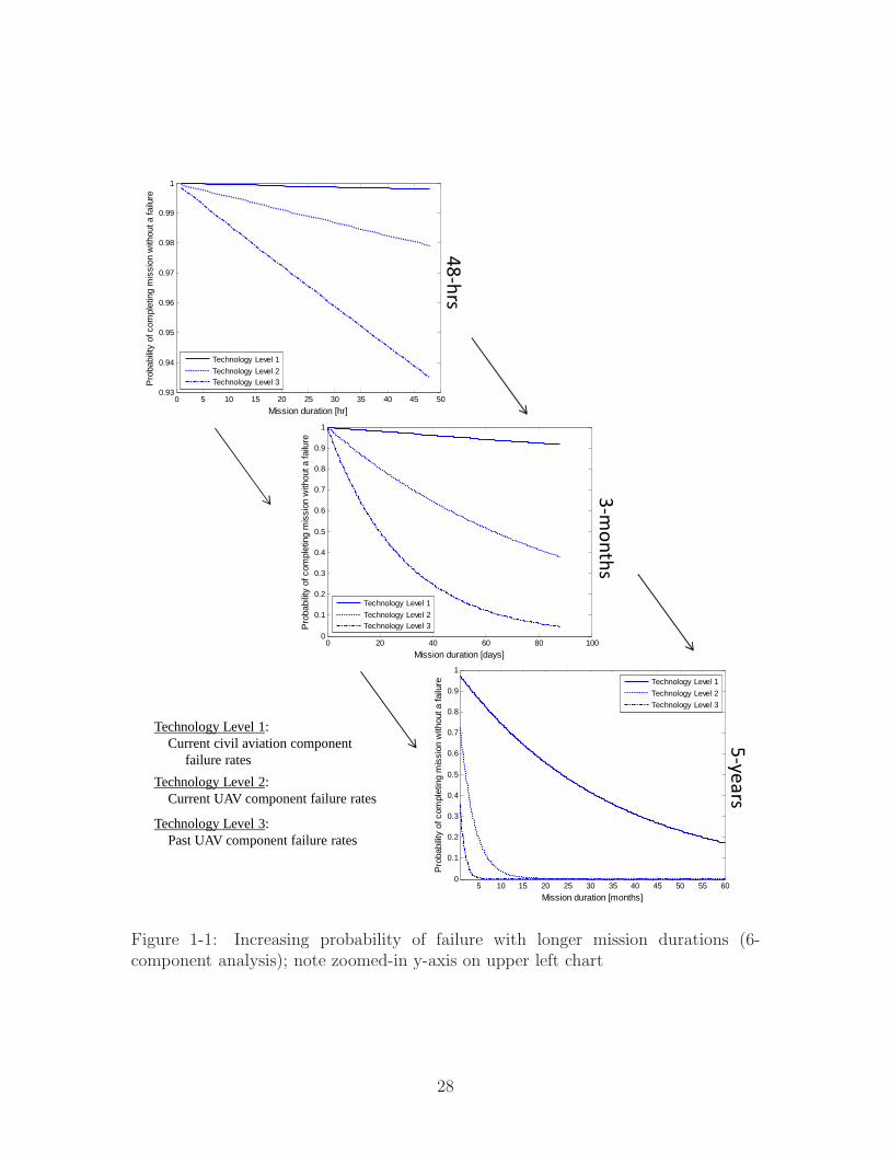
The above challenges pose a complex multistate design problem, the solution of
which is critical for ensuring high probability of mission success. Many of these sys-
tems may experience off-nominal conditions that dominate their operational period.
To gain an appreciation for this fact, consider the charts shown in Fig. 1-1. These
are computed using the Markov analysis described in Chapter 2, Section 2.3.2, and
show the probability that an aerial system will leave its nominal state of operation
over a given mission duration. It assumes three levels of failure rates for critical flight
control actuators and engines, which have been taken from several sources [36, 81, 84],
and will be discussed in following chapters.
There are two important observations to take from Fig. 1-1. The first is that
each of the three plots uses the same set of failure rates. When dealing with mission
durations on the order of one or two days, as in the upper left chart, these rates result
in very high probabilities of completing the mission without experiencing failures. In
all but the lowest technology level, representative of component reliabilities used in
UAV’s of the 1990’s, this probability is up near 99% or higher. For civil aviation, it
27
5 10 15 20 25 30 35 40 45 50 55 600
0.1
0.2
0.3
0.4
0.5
0.6
0.7
0.8
0.9
1
Mission duration [months]
Pro
babi
lity
of c
ompl
etin
g m
issi
on w
ithou
t a fa
ilure
Technology Level 1
Technology Level 2
Technology Level 3
0 20 40 60 80 1000
0.1
0.2
0.3
0.4
0.5
0.6
0.7
0.8
0.9
1
Mission duration [days]
Pro
babi
lity
of c
ompl
etin
g m
issi
on w
ithou
t a fa
ilure
Technology Level 1
Technology Level 2Technology Level 3
0 5 10 15 20 25 30 35 40 45 500.93
0.94
0.95
0.96
0.97
0.98
0.99
1
Mission duration [hr]
Pro
babi
lity
of c
ompl
etin
g m
issi
on w
ithou
t a fa
ilure
Technology Level 1
Technology Level 2Technology Level 3
48-hrs
3-months
5-years
Technology Level 1:Current civil aviation component
failure rates
Technology Level 2:Current UAV component failure rates
Technology Level 3:Past UAV component failure rates
Figure 1-1: Increasing probability of failure with longer mission durations (6-component analysis); note zoomed-in y-axis on upper left chart
28

is where one would expect, in the range of 99.9%. As the mission duration increases,
however, these same rates result in very poor probabilities of failure avoidance. In
the case of the five year duration, such as that proposed by DARPA’s Vulture pro-
gram, even the highest technology levels used in current civil aviation fall far short of
reasonable requirements. The development of such systems will require a paradigm
shift in aerospace design methodology.
The direction in which this shift should head is underscored by the second im-
portant observation. Namely, that the charts in Fig. 1-1 comment only on whether
or not the system will experience a failure of the engines or flight control actuators.
They say nothing about the system’s performance once that failure has occurred.
Nevertheless, traditional reliability analysis focuses primarily on preventing this fail-
ure from occurring, after the system has been designed to maximize performance in
the nominal state. As observed from the 5-year mission plot, the prevention of this
failure will likely be a losing battle. The solution proposed here is to accept that
failures will occur and integrate their performance into the early-phase design space.
This represents a shift away from seeking perfection, to pursuing adequacy, a difficult
paradigm shift for classically trained engineers.
A simple example hints at the potential effectiveness of using such an approach.
Consider the case of a dual-engine aircraft, such as that shown in Fig. 1-2. A more
Figure 1-2: 3-view of a twin-engine aircraft
detailed development of the case is given in Chapter 3, but for now assume the aircraft
29
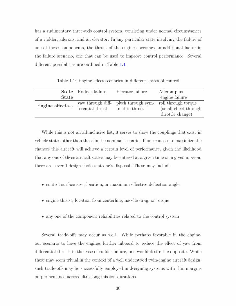
has a rudimentary three-axis control system, consisting under normal circumstances
of a rudder, ailerons, and an elevator. In any particular state involving the failure of
one of these components, the thrust of the engines becomes an additional factor in
the failure scenario, one that can be used to improve control performance. Several
different possibilities are outlined in Table 1.1.
Table 1.1: Engine effect scenarios in different states of control
State Rudder failure Elevator failure Aileron plusState engine failure
Engine affects...yaw through diff- pitch through sym- roll through torqueerential thrust metric thrust (small effect through
throttle change)
While this is not an all inclusive list, it serves to show the couplings that exist in
vehicle states other than those in the nominal scenario. If one chooses to maximize the
chances this aircraft will achieve a certain level of performance, given the likelihood
that any one of these aircraft states may be entered at a given time on a given mission,
there are several design choices at one’s disposal. These may include:
• control surface size, location, or maximum effective deflection angle
• engine thrust, location from centerline, nacelle drag, or torque
• any one of the component reliabilities related to the control system
Several trade-offs may occur as well. While perhaps favorable in the engine-
out scenario to have the engines further inboard to reduce the effect of yaw from
differential thrust, in the case of rudder failure, one would desire the opposite. While
these may seem trivial in the context of a well understood twin-engine aircraft design,
such trade-offs may be successfully employed in designing systems with thin margins
on performance across ultra long mission durations.
30
1.2 Summary of Relevant Research
The thesis approaches this problem by formulating it in terms of expected, or state
averaged, performance, rather than nominal performance, and in terms of the sys-
tem’s availability across its planned mission duration. The focus is on accurately
characterizing the multistate design space to ensure that the design/decision maker
has the information necessary to make informed choices concerning the system’s ro-
bust performance and to move this performance in a direction of improvement. The
following is an overview of relevant research, which will followed by a more detailed
review of literature in Chapter 2.
To date, the majority of design work done with regards to the robustness of multi-
state systems has occurred on three fronts, summarized here in the context of their
relevance to the proposed research. The first deals with systems where a certain pre-
dictable structure applies to the various levels of state performance (typically, but not
limited to, degraded performance in failure). This predictability allows performance
levels to be modeled by a single, or set of, structure functions and optimized as de-
scribed in Lisnianski [69]. Applicability is limited to simpler systems such as those
related to flow (e.g. pumping stations) or data transmission (e.g. circuit boards). In
aerospace systems, the complexity of interactions between disciplines and the much
larger space of performance metrics makes usefulness of such methods limited. The
second front focuses on control design and (dynamic) optimization to develop effi-
cient methods for dynamically determining the system’s state once in operation and
effectively controlling it to maximize mission performance. Into this category fall the
State Analysis methodology developed under NASA’s Mission Data System Frame-
work [66], work with hybrid systems, such as that at MIT described in [21], and a
broad range of work in developing fault tolerant systems. While the research in this
area is substantial and highly innovative, it deals predominantly with control, automa-
tion, and dynamic optimization as opposed to the parametric (static) optimization of
the system’s up-front design. The third front turns focus to the system’s reliability as
dependent on the failure rate (1/mean-time-between-failure) of its components and
31
subelements. Here, design has concentrated on analysis of how changes in these failure
rates affect overall performance and system availability and adjusting them accord-
ingly to maximize these two metrics. More recent work has concentrated on mapping
the effect of system faults into the corresponding performance space and recognizes
that reliability is an integrated systems problem, as described in Dominguez-Garcia
[39] and Babcock [9]. In light of this integrated problem, the above mentioned re-
search acknowledges the link between a system’s core design parameters and expected
performance in the face of degradation, but stops short of actually manipulating them
in a comprehensive manner such that robustness is improved.
There are several reasons why the above solutions have not pushed beyond the de-
scribed limitations. Many of these have to do with the effort of meeting the challenges
presented by the multistate design problem, which includes: 1) multiple performance
levels characterized by the duration of time the system spends in any particular state
and their relative importance in terms of mission achievement, 2) competing trade-offs
between states’ maximum performance levels, and 3) potentially high dimensional-
ity resulting from the evaluation of numerous states. With mission scenarios char-
acterized by longer durations, more demanding environments, infrequent or costly
maintenance opportunities, and tight fiscal constraints, the benefits of a more com-
prehensive and integrated approach to the early stage design become more attractive.
Fortunately, each of the challenges are particularly suitable for the integrated analy-
sis afforded by modern multidisciplinary analysis tools. These tools include various
techniques for organizing coupled design problems of high dimensionality into smaller,
more tractable sub-problems, as well as:
• Sensitivity analysis w.r.t. static design variables, both at the component/discipline
level and at the coupled, system level
• Sensitivity analysis of optimum w.r.t. parameters
• Radical reduction of computational elapsed times by the use of surrogate models
and parallel computing
• Many Design of Experiment (DOE) techniques for efficient sampling of the
32

design space and subsequent analysis of performance effects
This thesis extends the above sensitivity analyses to include the integrated effects
of component failures rates, as well as static design variables. Where possible, it
uses parallel computing for the evaluation of individual state performances, and adds
to the surrogate modeling techniques a surrogate formulation for system availability.
Finally, several DOE techniques are used throughout the case studies in the analysis
and visualization of the multistate design space.
1.3 Thesis Contributions
As mentioned above, research into the design and optimization of multistate systems
has typically focused on 1) systems with a predictable state performance structure,
commonly referred to as multistate coherent systems, 2) control design and optimiza-
tion, and 3) improvements in component failure rates and redundancy (reliability
analysis). Fig 1-3 shows how the thesis fits within the current field of research de-
fined in this context. Chapter 2 reviews the literature of multistate design in more
detail as well as relevant research in multidisciplinary analysis and optimization.
The research goal is to propose and demonstrate an integrated multistate method-
ology early in the design process that improves expectation of the system’s success
over long mission durations. Key contributions of this work include:
• The development and demonstration of the central methodology, in the form of
an integrated multistate design approach that formulates responses of system
expected performance and availability as functions of static design variables
(geometry) and component failure rates, accounting for control design variables
(gains) where appropriate.
• Demonstration of the cost and benefits, in the form of design trade-offs, associ-
ated with a multistate design approach as compared to pure reliability analysis
techniques and the nominal design approach.
33

Syste
m Co
mplex
ity
System Life
ControlDesign &
AutonomousOperationsMultistate
CoherentSystems
Reliability Analysis
Thesis Research
Figure 1-3: Fields related to multistate design
• A multilayer approach, using Markov analysis, for translating single sortie ve-
hicle level metrics into measures of multistate campaign performance.1
• A surrogate function for system availability that allows the otherwise piecewise-
constant metric to be optimized via gradient-based optimization algorithms.
• Major findings of the thesis, including evidence of:
– multistate performance output spaces having distinctly unique shapes and
boundaries, depending on whether formed through variation of component
failure rates, static design variables (geometry), or a multistate combina-
tion of both,
– a region of multistate performance resulting from the combined variation
of failure rates and static design variables that is unachievable through the
independent variation of either one,
1Sortie refers to a single operational return trip of the vehicle, while campaign refers to a collectionof sortie operations for a single objective.
34

– small changes in static design variables that may be used to significantly
improve system availability, and
– the general multistate design problem being one of competing objectives
between system availability, expected performance, nominal performance,
and cost.
In addition to the above contributions, the thesis develops some general principles
concerning multistate analysis and design in the early-phase development of complex
systems. These are described in detail in Chapter 7, and listed below for preliminary
reference:
1. The general multistate problem is a multi-objective one with com-
peting trade-offs between nominal performance, system availability,
expected performance, and cost.
2. The systems benefiting most from multistate analysis and design are
systems with long operational durations and little opportunity for
maintenance or repair, and systems involved in multi-system opera-
tions where costs of downtime and system loss are high.
3. Using component failure rates to increase availability or expected
performance will tend to increase direct system cost, while using
static design variables for the same can either increase or decrease
this cost.
4. In multistate system design, time often plays the role of both objec-
tive and constraint.
The last principle is especially true in the case of multistate long endurance sys-
tems, where the objective performance metric is to stay in operation as long as pos-
sible. As the improving design lengthens this period of operation, the probability
distribution of performance begins migrating from the nominal state into the off-
nominal states. Simply put, the longer the system’s endurance, the longer the period
35

between maintenance opportunities, and the higher the chance of experiencing off-
nominal states. Although the last principle seems to be common sense, it is a fact
that many designers not familiar with reliability analysis might overlook. By the time
the design makes it to the reliability engineers, it has already passed the point where
useful improvement to the system’s availability may be effected through static design
variables. This is one of the key issues addressed by the thesis.
1.4 Thesis Overview
The research presented in this thesis began with a review of literature from several
fields dealing with the topic of multistate design. Next, a well-known and validated
aircraft design case was used to show the feasibility of using static design variables
as an effective means of improving expected performance and system availability. A
more formalized methodology was then developed, based on lessons from the first
case study, and applied to the design of a long endurance UAV and the lubrication
system for a geared turbofan engine.
Fig. 1-4 presents a comprehensive overview of the dissertation in the form of an
Object-Process Diagram (OPD) [41]. Here, boxes depict objects (highlighted boxes
are main objects, all others are supporting objects), ovals depict processes, unidirec-
tional arrows indicate execution of a process resulting in an object, and circle-ended
lines show linkages between processes and their supporting objects. Bidirectional
arrows indicate two-way relationships between entities.
The following paragraphs give a detailed chapter-by-chapter summary:
Chapter 2. The main contributions of this chapter are the detailed presentation of
the basic concepts and definitions in multistate design, and the extension of this from
relatively simple systems to more complex aerospace systems. The chapter begins
with a detailed review of literature, coming predominantly from the fields of design
optimization, reliability analysis, and controls design. The remainder of Chapter 2
provides an in-depth discussion of multistate design. Some of this has been extracted
36

Chapter 1
Chapter 4
Chapter 3
Chapter 2
Chapter 5 Chapter 6
Chapter 7
Markov ReliabilityAnalysis
Flight Test Data
Control Design
Design of Experiments
(DOE)
Propulsion/Engine Design
Reviewing
Motivating
SummarizingIdentifying
Gap
Defining
ReliabilityLiterature
Design Optimization
Literature
ControlsLiterature Multistate
Literature
Understanding
Analyzing
Validating
Generalizing
Formulating
Applying
Demonstrating
Drawing Conclusions
Comparing
SummarizingRecommending
Motivation, overview, and research gap
Long Duration Systems
SensitivityAnalysis
Multistate Design & Analysis
AircraftDesign
ReliabilityDesign
Background, definitions, & modeling
Feasibility: Twin-engine aircraft
Methodologyformulation
Application: Ultra –long endurance UAV
Application: GTF Engine lubrication system
Conclusions & future work
Figure 1-4: Object-Process Diagram presentation of thesis
37

from the very small body of formal multistate design literature, dealing with relatively
simple systems, and much has been modified/extended to the case of more complex
aerospace systems. Markov modeling, as it pertains to traditional reliability analysis,
is discussed and its nomenclature integrated with that of the multistate processes
described in the thesis.
Chapter 3. Chapter 3 demonstrates feasibility of the multistate approach through
the design analysis of an existing twin-engine aircraft. The chapter begins to inte-
grate elements for determining responses in expected performance and availability to
changes in static design variables (geometry), control design variables (gains), and
component failure rates, considered the three driving input categories affecting the
aircraft’s performance robustness. Key results from the twin-engine aircraft study
show that, while many unsatisfactory geometry-state responses occur in the fully
failed state and are expected, several occur in partially degraded states where the
majority of geometries are able to meet performance requirements. This behavior
clearly exhibits itself in the resulting design sensitivities, confirming that such an
approach allows designers to identify elements that might drive system loss through
analysis of performance changes across system states, and their respective response to
changes in static design variables. The effectiveness of the basic methodology demon-
strated in this chapter sets the stage for a more in-depth methodological formulation
in Chapter 4, and the methodology’s application to case studies in Chapters 5 and 6.
A large part of the research and results from Chapter 3 have been recommended for
publication in [1].
Chapter 4. The main contributions of this chapter include:
• A generalized methodology for multistate analysis and design, shown in Fig. 1-5.
• A multilayer extension of Markov analysis, for translating single sortie compo-
nent and vehicle level availability to multiple sortie mission campaign robust-
ness.
• The development and demonstration of a “surrogate” function for system avail-
38

ability.
The chapter begins with the development of the generalized methodology for mul-
tistate analysis and design, based upon its effectiveness as demonstrated in Chapter 3.
In support of this framework, the chapter continues with the description of a multi-
layer Markov analysis technique that enables the calculation of campaign performance
and vehicle attrition as a function of component failure rates and vehicle static design
variables.
������
������� ���� ��������� ���� �� ��������������START
Requirements Definition,
Concept of Operations
Classification of System
and Performance Metric
INPUT to computational analysis
Modelingand
Simulation
ParallelProcessing/SurrogateModeling
MarkovAnalysis ������������ �����
OUTPUT from computational analysis
Analysis/Visualization
PreliminaryFailure Modes
Analysis
Architectural Decision(s)
� ��� ������������������������������ � ������������ �� ���� ����� ���� �����������������YES
update
NO
YES
NOFINISHED
update
c ��� ��� �� ���������� ����������x ��� ��� �� ����� ��������� λ � �������� ������ �����
MultistateDesign
Framework
1. 2.
3.
4.
5.
6.
Figure 1-5: A framework outline for multistate design
Chapter 4 concludes with a discussion of issues in multistate optimization, which
may occur as part of the computational analysis. This includes the special case of
system availability, essentially a piecewise constant function in which improvement
corresponds directly to increasing performance in off-nominal states above a certain
threshold. A surrogate function is formulated that allows for the improvement of
expected availability through gradient-based optimization methods.
39

Chapter 5. The methodologies formalized in Chapter 4 are applied to the design and
analysis of a long endurance unmanned aerial vehicle in this chapter. Key findings
from this case study show that:
• Each performance space stemming from three distinct design approaches (vary-
ing only failure rates, varying only static design variables, or combined multi-
state variation of both) has distinctly unique shapes and boundaries.
• The achievable improvement in system availability via static design variables is
nearly as large as that made via component failure rates. From the perspective
of reliability analysis, this is significant due to the fact that improvements in
reliability are nearly always sought after through changes in component failure
rates, rather than affecting state performance through changes to static design
variables.
• Perhaps most importantly, the inclusion of both static design variables and com-
ponent failure rates in the design analysis allows a region of system availability
to be reached that is unobtainable via the independent variation of either one.
The combined multistate approach demonstrated an improvement in system avail-
ability of 11%, at a 3% lower cost, when compared to the baseline UAV designed for
nominal performance. Variation of component failure rates or static design variables
alone showed an improvement of only 6.5%. Furthermore, when considering mul-
tiple objectives of system availability, expected performance, nominal performance,
and cost, the combined approach was still able to achieve an 11% improvement in
availability, with only a 4.5% decrease in nominal performance, albeit at a small 6%
increase in aircraft flyaway cost.
Chapter 6. This chapter complements Chapter 5 by demonstrating application of
multistate analysis and design to a lower level aerospace subsystem. The case study
is the lubrication system for a high bypass ratio geared turbofan (GTF) engine in the
20,000- to 30,000-lbf thrust class. Key findings demonstrate that:
• Even in the simpler design space characterized by the lubrication subsystem,
40

sensitivity of expected performance to changes in static design variables varies
significantly between the nominal case and two multistate scenarios of differing
time duration. In one case, the sign of the sensitivity even reverses trend. The
impact of this is that, designing for best performance in the nominal scenario,
while affecting availability only through component failure rates, will likely re-
sult in an inferior multistate design.
• The surrogate function for availability proves effective within a gradient-based
algorithm for generation of Pareto fronts.
• Variation of static design variables alone led to improvement of subsystem avail-
ability by 22% over a time duration of 500-hrs (Fig. 6-11). When considering
oil system cooling size as a representation of cost, and adjusting accordingly,
the best Pareto solution still resulted in an improvement of 10%.
This case study is successful in demonstrating how specific changes to the lubrica-
tion system’s design improve the robustness of its performance across several modes
of failure. Additionally, the methodology is demonstrated such that it may be ex-
tended to a more detailed multistate analysis given higher fidelity tools and models
available to engine industry experts.
Chapter 7. The final chapter summarizes key results of the thesis. It draws together
major findings and conclusions arising from the three central case studies, and uses
these to develop some general principles for early-phase multistate analysis and de-
sign. Finally, the chapter recommends areas of research for further improvement in
multistate design, outlining a performance space mapping approach for reducing the
high computational burden of the multistate problem.
41

42

Chapter 2
Understanding Multistate Design
Chapter 2 presents the basic concepts and existing research in multistate design,
and lays the foundation for modeling multistate systems. The first section reviews
literature in the three main areas of current multistate design research. Next, mul-
tistate design is defined within the scope of the thesis, followed by the development
of multistate nomenclature and terminology used throughout the remainder of the
dissertation. The remaining sections deal with the modeling of state transitions,
introducing Markov chains, and several issues of multistate performance modeling.
2.1 Review of Literature
Research into the analysis and design of multistate systems has typically focused
on 1) systems with a predictable state performance structure, 2) control design and
optimization, and 3) improvements in component failure rates and redundancy. This
section reviews the literature of multistate design in more detail as well as relevant
research in multidisciplinary design optimization.
2.1.1 Multistate Coherent Systems
There are many systems where a certain predictable structure applies to the various
levels of state performance. These are often comparatively simpler systems such as
43
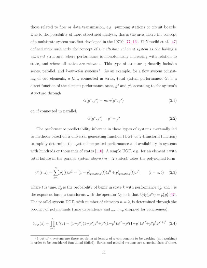
those related to flow or data transmission, e.g. pumping stations or circuit boards.
Due to the possibility of more structured analysis, this is the area where the concept
of a multistate system was first developed in the 1970’s [77, 16]. El-Neweihi et al. [47]
defined more succinctly the concept of a multistate coherent system as one having a
coherent structure, where performance is monotonically increasing with relation to
state, and where all states are relevant. This type of structure primarily includes
series, parallel, and k -out-of-n systems.1 As an example, for a flow system consist-
ing of two elements, a & b, connected in series, total system performance, G, is a
direct function of the element performance rates, ga and gb, according to the system’s
structure through
G(ga, gb) = min{ga, gb} (2.1)
or, if connected in parallel,
G(ga, gb) = ga + gb (2.2)
The performance predictability inherent in these types of systems eventually led
to methods based on a universal generating function (UGF or z -transform function)
to rapidly determine the system’s expected performance and availability in systems
with hundreds or thousands of states [110]. A simple UGF, e.g. for an element i with
total failure in the parallel system above (m = 2 states), takes the polynomial form
U i(t, z) =
m∑
k=1
pik(t)zgik = (1− pioperating(t))z
0 + pioperating(t)zgi ; (i = a, b) (2.3)
where t is time, pik is the probability of being in state k with performance gik, and z is
the exponent base. z transforms with the operator δG such that δG(pikz
gik) = pikg
ik [67].
The parallel system UGF, with number of elements n = 2, is determined through the
product of polynomials (time dependence and operating dropped for conciseness),
Usys(z) =
n∏
i=1
U i(z) = (1−pa)(1−pb)z0+pa(1−pb)zga+pb(1−pa)zgb+papbzga+gb (2.4)
1k -out-of-n systems are those requiring at least k of n components to be working (not working)in order to be considered functional (failed). Series and parallel systems are a special class of these.
44
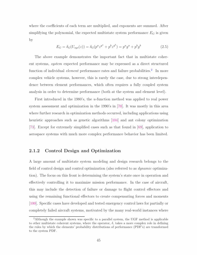
where the coefficients of each term are multiplied, and exponents are summed. After
simplifying the polynomial, the expected multistate system performance EG is given
by
EG = δG(Usys(z)) = δG(pazg
a
+ pbzgb
) = paga + pbgb (2.5)
The above example demonstrates the important fact that in multistate coher-
ent systems, system expected performance may be expressed as a direct structured
function of individual element performance rates and failure probabilities.2 In more
complex vehicle systems, however, this is rarely the case, due to strong interdepen-
dence between element performances, which often requires a fully coupled system
analysis in order to determine performance (both at the system and element level).
First introduced in the 1980’s, the u-function method was applied to real power
system assessment and optimization in the 1990’s in [70]. It was mostly in this area
where further research in optimization methods occurred, including applications using
heuristic approaches such as genetic algorithms [104] and ant colony optimization
[73]. Except for extremely simplified cases such as that found in [69], application to
aerospace systems with much more complex performance behavior has been limited.
2.1.2 Control Design and Optimization
A large amount of multistate system modeling and design research belongs to the
field of control design and control optimization (also referred to as dynamic optimiza-
tion). The focus on this front is determining the system’s state once in operation and
effectively controlling it to maximize mission performance. In the case of aircraft,
this may include the detection of failure or damage to flight control effectors and
using the remaining functional effectors to create compensating forces and moments
[100]. Specific cases have developed and tested emergency control laws for partially or
completely failed aircraft systems, motivated by the many real-world instances where
2Although the example shown was specific to a parallel system, the UGF method is applicableto other multistate coherent systems, where the operator, δ, takes a more complex role in definingthe rules by which the elements’ probability distributions of performance (PDF’s) are transformedto the system PDF.
45

such control laws may have been helpful [26, 43]. Burcham et al. [27] documents the
extensive development and evaluation of an emergency flight control system for an
F-15 using only differential thrust. Results from the 36-flight evaluation showed that
such a system can be used to successfully land an aircraft that has suffered from a
major flight control system failure. A similar endeavor in Monaco et al. [111] details
the successful retrofitting of an F/A-18 with a model-based adaptive control sys-
tem to respond to states brought about by flight control failure, damage, or adverse
environmental conditions.
Oriented more towards space systems, this category also includes the State Anal-
ysis methodology developed under NASA’s Mission Data System (MDS) Framework
[66, 60]. The goal of State Analysis is to “improve the current state-of-the-practice by
producing requirements on system and software design in the form of explicit models
of system behavior, and by defining a state-based architecture for the control system”
[58]. Figure 2-1 is a diagram taken from Dvorak et al. [46] showing how the method-
ology attempts a unified approach to system analysis, control system software design,
and system operation.
Figure 2-1: State Analysis methodology
Work with the MDS framework and State Analysis has also been successfully
46

applied in conjunction with advances in the area of hybrid system control optimization
[24]. Hybrid systems are those which exhibit both continuous state and discrete state
dynamics, a category into which most aerospace systems fall. Some examples of work
in this area include control optimization for robust execution in the face of uncertainty
[21], extension of the branch and bound method in solving hybrid discrete/linear
optimization problems [68], and an investigation into the complexity of hybrid system
optimization when transformed into a mixed-integer linear programming problem
[107]. An excellent review and introduction to hybrid systems control is given in
Labinaz [65]. Research in this area is substantial and highly innovative, dealing
predominantly with control, automation, and dynamic optimization rather than the
parametric (static) optimization of the system’s up-front physical design.
2.1.3 Design for Reliability
This third front turns focus to the system’s reliability through the failure rate of its
components and sub-elements. A great deal of successful work has used integrated
system modeling with Markov models to determine the system reliability (and system
availability) of large, complex systems performing life-critical applications [9, 11].
Markov analysis ensures that highly improbable states and the events leading up to
those states are accurately measured and tracked. A generic Markov state transition
diagram is depicted in Figure 2-2, shown here for multiple states of failure without
repair. The diagram is read from left to right, starting from the nominal state to
states with increasingly serious failures.
In this formulation, the probability PK that the system finds itself in any partic-
ular state of performance GK (at time t) can be determined by solving a system of
differential equations derived from the transition probabilities Pr. These transition
probabilities, in the case of failures, are typically derived from known values of com-
ponent or element mean-time-between-failure (MTBF). The simplest formulation for
the failure rate results in Pr...−K = λi, where λi is the inverse of the MTBF for the
ith component. Coupled with the integrated system model, the methodology enables
determination of how overall system availability and performance change in response
47

� ! "
#$% &"""
'()*+'()*,'(+*-'+*.'(,*/'(,*0
'(-*111'(.*111'(/*111'(0*23) 3+ 3-
3,3.3/30
30303034Figure 2-2: Markov state transition diagram
to variation of component failure rates and time.
The motivation for this thesis originally developed in response to the sponsor’s
need for expanding this type of reliability analysis beyond that involving just com-
ponent failure rates. Recent work in Dominguez-Garcia [39, 40] has moved in this
direction by merging system behavioral analysis with the integrated Markov model
generation described in [10], allowing evaluation of performance for multiple system
events (e.g. multiple failures and/or sequences of failures). By mapping the effect of
system faults into the appropriate performance space, the research acknowledges the
link between a system’s core design variables and expected performance in the face of
degradation, but stops short of manipulating them in a comprehensive manner such
that robustness is improved.
Finally, there are many mature techniques to represent multistate systems for the
evaluation of reliability. These include fault trees, block diagrams, dynamic fault
trees [45], as well Markov models, some of which have been extended to relatively
complex phased-mission analyses [96]. Literature is extensive on the topic, but a good
overview can be found in [56, 87]. Most of these techniques require the analyst to
specify which states are classified as ‘failed’, often using qualitative descriptions of the
system’s functionality. Some are more easily adapted to quantitative analysis (such
as Markov models) than others, allowing the integration of analytical or simulation-
48

based performance into the overall system reliability model.
2.1.4 Relevant Methods in Multidisciplinary Design
Optimization
Multidisciplinary Design Optimization (MDO) encompasses a body of algorithms, for-
mulations, and techniques that facilitates the efficient design of engineering systems.
These systems are influenced by different physical interacting phenomena, which are
aligned with different engineering disciplines. Decomposition into disciplines or sub-
elements is often needed. Many of these tools are appropriate for the solution of
the multistate problem, as well. Although its roots lie in structural optimization,
the past two decades have seen MDO’s increasing use across numerous engineering
fields. Several sources provide reviews of the topic, some of the more recent are Ted-
ford and Martins [105], Alexandrov [4], and Agte et al. [3]. More dated, but very
comprehensive is Sobieszczanski-Sobieski and Haftka [98].
Formal MDO notation generally follows that of the Nonlinear Programming (NLP)
format, where the optimization problem is stated as Eqn. 2.6:
given c = [c1, ..., cnc]
minimize J = f(x, c)
x = [x1, ..., xnx]
s.t. h(x, c) = 0
g(x, c) ≤ 0
xi,LB ≤ xi ≤ xi,UB, i = 1, 2, ..., nx
(2.6)
where c is a vector of fixed parameters that influence the behavior of the system
(material properties, operating conditions, etc.), f is the function to be minimized,
x is a non-dimensional vector of static design variables with lower and upper bounds
(may be either continuous or discrete), and h and g are equality and inequality
constraints, respectively. J can be also be a vector of multiple objectives.
49

The formulation in Eqn. 2.6 proves very effective in solving problems of multistate
performance. Most notable is its usefulness in refining the constrained design for sys-
tem availability and expected performance, as demonstrated in Eqn. 5.5 of Chapter 5,
and in forming the dual objective Pareto fronts of Section 6.7.2 in Chapter 6.
In addition to the NLP single optimization loop, shown in Figure 2-3 for reference,
the MDO problem may also be organized into a decomposed structure such as that
shown in Figure 2-4.
Analysis Code
Optimizer
x5x678 x9
f:, g6,h6initialguess
convergence criterion
optimaldesign
Figure 2-3: NLP - single optimization loop[3]
System Optimizer Analyzer 1Optimizer 1
Optimizer 2
Optimizer 3
fxy;<*,y=<*y<;*,y<=*y<=*,y;=*
Analyzer 2
Analyzer 3
x<d< y<;,y<=g<,f<x;d; y;<,y;=g;,f;x=d= y=<,y=;g=,f=
Figure 2-4: MDO problem decomposedinto two levels - NAND @ disc. level,SAND @ sys. level [12]
Balling and Sobieski [12] describe the fundamental MDO approaches as follows:
The fundamental approaches to MDO formulation vary in two aspects.
First is the distinction between single-level optimization and multilevel
optimization. In multilevel optimization approaches, the disciplinary de-
sign variables are determined by disciplinary optimizers and the system
design variables are determined by the system optimizer. In single-level
optimization approaches, both disciplinary and system design variables
are determined by the system optimizer. Second is the choice between
simultaneous analysis and design (SAND) and nested analysis and design
50
(NAND). This distinction can be made at both the system and the dis-
cipline levels. At the discipline level, SAND implies that the disciplinary
design and state variables are determined simultaneously by the optimizer,
whereas NAND implies that the optimizer determines only the disciplinary
design variables and requires determination of the state variables at each
iteration.
There are several decomposition methods derived from the above elements in
conjunction with data organization structures such as the design dependence matrix
(a.k.a. N -square diagram, N2, or design structure matrix, DSM, described in Stewart
[102]). Other tools that have seen very successful use in MDO include many Design of
Experiment (DOE) and sensitivity analysis processes for effective exploration of the
design space. This thesis uses the DOE methods of Latin-hypercube spacing [62] and
orthogonal arrays [54] for efficiently sampling the design space for maximum coverage
and determining the effects of design variables on performance output. Both of these
methods are described further in Chapters 5 and 6, respectively.
Sensitivity analysis may be used at different system levels and stages of the de-
sign process to provide invaluable information to the designer concerning any number
of outputs. This may include: System Sensitivity Analysis (SSA) [97], Subsystem
Sensitivity Analysis (SSSA) [52], sensitivity analysis of optimum w.r.t parameters, or
post-optimum sensitivity analysis [17]. The above make possible the thorough map-
ping of gradient information from the system level all the way down to the component
level. Typically, this gradient information is only calculated for the effects of the sys-
tem’s static design variables. For multistate analysis and design, the above sensitivity
analyses are extended to include the integrated effects of component failures rates, as
well as the static design variables.
Finally, in addition to gradient-based methods, many heuristic algorithms have
become very powerful when used in the context of multidisciplinary design optimiza-
tion. These include genetic algorithms [72], simulated annealing [93], and particle
swarm optimization [15], to name a few. A large amount of work has combined both
gradient and heuristic methods to improve very complex designs [50, 6] in a pro-
51
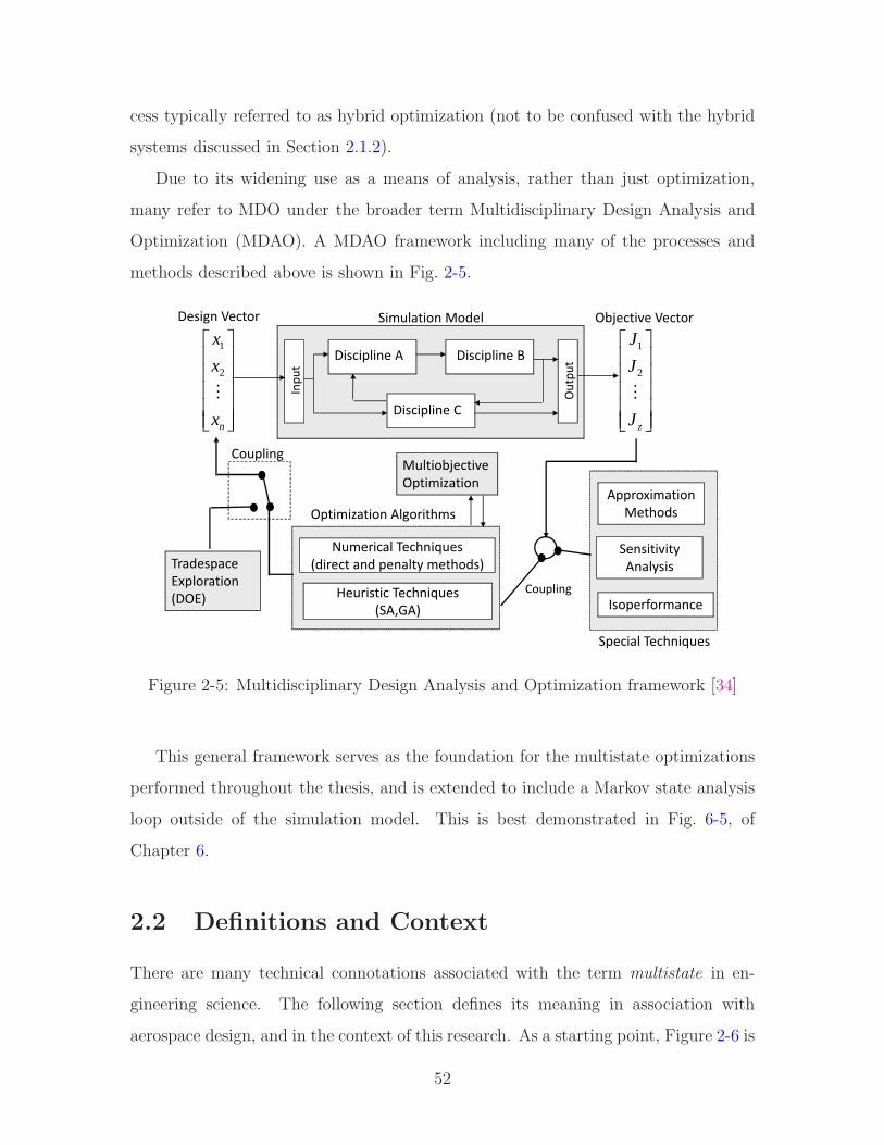
cess typically referred to as hybrid optimization (not to be confused with the hybrid
systems discussed in Section 2.1.2).
Due to its widening use as a means of analysis, rather than just optimization,
many refer to MDO under the broader term Multidisciplinary Design Analysis and
Optimization (MDAO). A MDAO framework including many of the processes and
methods described above is shown in Fig. 2-5.
Discipline A Discipline B
Discipline C
Simulation Model
TradespaceExploration(DOE)
Optimization Algorithms
MultiobjectiveOptimization
Numerical Techniques(direct and penalty methods)
Heuristic Techniques(SA,GA)
1
2
n
x
x
x
M
Design Vector
Coupling
1
2
z
J
J
J
M
ApproximationMethods
Coupling
Sensitivity Analysis
Isoperformance
Objective Vector
Special Techniques
Figure 2-5: Multidisciplinary Design Analysis and Optimization framework [34]
This general framework serves as the foundation for the multistate optimizations
performed throughout the thesis, and is extended to include a Markov state analysis
loop outside of the simulation model. This is best demonstrated in Fig. 6-5, of
Chapter 6.
2.2 Definitions and Context
There are many technical connotations associated with the term multistate in en-
gineering science. The following section defines its meaning in association with
aerospace design, and in the context of this research. As a starting point, Figure 2-6 is
52

proposed as a novel view on system state change hierarchy, organized according to the
distinct means by which the state of a particular aerospace system may potentially
change or be changed. Note that continuous or discrete state changes are not ruled
out at any particular level, although continuous states typically dominate at the lower
levels while discrete states dominate the higher. This is due mainly to the fact that
the upper two levels require the ceasing of operations in order to change state, while
the lowest levels allow the possibility of online state change via continuous variation
of controls.
Hierarchy of System State Change
V
IV
III
II
I
>?@? ABCCD@ ACEFG@H@GIJ>KK@L@MH J@D>NM>?@? DHCF CF@LOH>CM HCL@ACMK>NPL@QECJ>KIQPFNLOJ@>?@? ABOMN@ >M FBID>AOG N@CRE@HLI CL E@ABOM>AD SEOI T@AOPD@J TI DCKHUOL@ KO>GPL@DV>?@? HPM>MNW E>MCL DCKHUOL@@X@LA>D@J ABOMN@D>?@? HBLCHHG@W TLOY@ FL@DDPL@WDH@@L>MN OMNG@W LTI HB@CLICo
ntin
uous
stat
es d
omin
ate
Changing of controlsw/in prescribed limits
Expansion/movementof control limits
State change duringoperation
State changewhile offline
Use of uniquelydifferent design
Disc
rete
stat
es d
omin
ate
Figure 2-6: Hierarchy of system state change
At the most general level, shown as Level I, any system to which adjustments may
be made in order to modify performance could be characterized as having multiple
states. A pilot at the departure end of a runway changes the state of the aircraft by
53

using the throttle to increase fuel flow rate in order to take off. The flight control
system then constricts movement limits on control surfaces as the aircraft accelerates
(Level II ). At Level III, the aircraft’s state further changes when the pilot retracts the
flaps upon reaching a safe climb altitude. State transitions at Level IV and Level V
occur when the system must be taken out of operation in order to make configuration
changes or to meet requirements with an entirely different design.
Level III is the region where hardware or software failures may lead to state
transitions and the area where this research focuses. More specifically, these states
have distinct performance levels, brought about by discrete changes in the system
occurring at stochastically predictable points in continuous time. They occur while
the system is operating. The fact that they are stochastically predictable allows their
inclusion in the early-stage design loop, given that one can accurately model their
performance and efficiently handle the extra computational burden.
With the above in mind, three succinct definitions arise, defined here within the
specific context of this thesis:
• state: a discrete condition of the system, brought about by a discrete change
in the performance rate (e.g. operating ⇒ failed) of one or more elements that
compose that system.
• multistate system: a system subject to the above defined states, where each
state is a member of the set composed of all possible permutations of its ele-
ments’ performance rates.
• robust system: a system that consistently achieves satisfactory performance
across a broad range of operating conditions for a predicted set of system states,
including partially degraded states.
The above definitions of state fall more in line with the traditional terminology
used in reliability analysis [22, 69], than with that used in controls theory, where these
might often be referred to as operating modes.
54
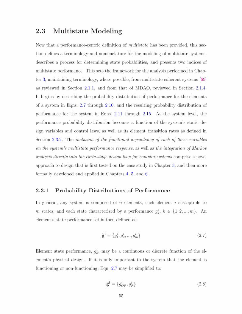
2.3 Multistate Modeling
Now that a performance-centric definition of multistate has been provided, this sec-
tion defines a terminology and nomenclature for the modeling of multistate systems,
describes a process for determining state probabilities, and presents two indices of
multistate performance. This sets the framework for the analysis performed in Chap-
ter 3, maintaining terminology, where possible, from multistate coherent systems [69]
as reviewed in Section 2.1.1, and from that of MDAO, reviewed in Section 2.1.4.
It begins by describing the probability distribution of performance for the elements
of a system in Eqns. 2.7 through 2.10, and the resulting probability distribution of
performance for the system in Eqns. 2.11 through 2.15. At the system level, the
performance probability distribution becomes a function of the system’s static de-
sign variables and control laws, as well as its element transition rates as defined in
Section 2.3.2. The inclusion of the functional dependency of each of these variables
on the system’s multistate performance response, as well as the integration of Markov
analysis directly into the early-stage design loop for complex systems comprise a novel
approach to design that is first tested on the case study in Chapter 3, and then more
formally developed and applied in Chapters 4, 5, and 6.
2.3.1 Probability Distributions of Performance
In general, any system is composed of n elements, each element i susceptible to
m states, and each state characterized by a performance gik, k ∈ {1, 2, ..., m}. An
element’s state performance set is then defined as:
gi = {gi1, gi2, ..., gim} (2.7)
Element state performance, gik, may be a continuous or discrete function of the el-
ement’s physical design. If it is only important to the system that the element is
functioning or non-functioning, Eqn. 2.7 may be simplified to:
gi = {giOP , giF} (2.8)
55

where OP indicates the operational state, F indicates failed state, and m = 2. This
simplification by no means implies that the system composed of elements i has only
two states or two levels of performance.
In the multistate system, the performance gi of element i at any point in time,
t ≥ 0, is a value randomly taken from gi : gi(t) ∈ gi. Thus, across a system’s mission
time interval [0,T], an element’s, and consequently, the system’s performance may be
defined as a stochastic process. Often there exist means of stochastically determining
when and through what mechanism an element will occupy state k. Methods for
doing this will be discussed in the next section, but for now it is sufficient to say
that the probabilities associated with the state an element occupies at time t may be
represented as the set:
pi = {pi1(t), pi2(t), ..., pim(t)}, where pik = Pr{gi(t) = gik} (2.9)
This corresponds directly to the element’s state performances in Eqns. 2.7 or 2.8. The
state probability and performance pairs, {[pi1(t), gi1], [pi2(t), gi2], ..., [pim(t), gim]} com-
prise the entire probability distribution of performance for the element i at time, t.
Note that the element states arise from the entire set of mutually exclusive transitions
that can occur, therefore,
m∑
k=1
pik(t) = 1 for 0 ≤ t ≤ T (2.10)
Up to this point, little has been said about the system’s performance. In the case
of the multistate coherent systems described in Section 2.1.1, the determination of
performance for a system composed of n elements i follows directly from the individual
state performance of its elements. In the case of much more complex systems, the
system performance is a more complicated function of state, system static design
variables, x, control laws, r, and operational parameters, c. Note that x and c
were previously defined for Eqn. 2.6 of Section 2.1.4, and r is a general variable that
represents targeted variation to the system’s control laws, e.g. gains.
56

The determination of system state (as opposed to performance), however, is made
directly from the state of the elements. Consider that the system, composed of n
elements i, has M states, each state with performance GsK(x, r, c), K ∈ {1, 2, ...,M},
such the set of system state performances may be represented as:
Gs = {Gs1(x, r, c), G
s2(x, r, c), ..., G
sM(x, r, c)} (2.11)
The system performance, Gs(t), is a random value drawn from the family of functions
Gs : Gs(t) ∈ Gs
The system states K are determined by the possible permutations of the elemental
states k. The number of system states, M , depends on the rules that govern those
permutations. For instance, the total number of system states will be much greater
if the emerging performance levels, GsK , are dependent on the order of element state
transition in addition to just their states (i.e. system performance is different when
element i transitions before i+1 vs. i+1 before i). When order is not important and
the element performance set is limited to the failure case of Eqn. 2.8, the size of M
is equal to 2n (n is the number of elements). If the emergent performance is order
dependent, the total number of states is,
1 +
n∑
j=1
n!
(n− j)!(2.12)
In either case, one can see that the total number of system states grows very rapidly,
even when the number of element states, m is limited to two.
As with the elements, there exists a corresponding set of system state probabilities,
Ps = {P s1 (t), P
s2 (t), ..., P
sM(t)}, where P s
K = Pr{Gs(t) = GsK} (2.13)
such thatM∑
K=1
P sK(t) = 1 for 0 ≤ t ≤ T (2.14)
57
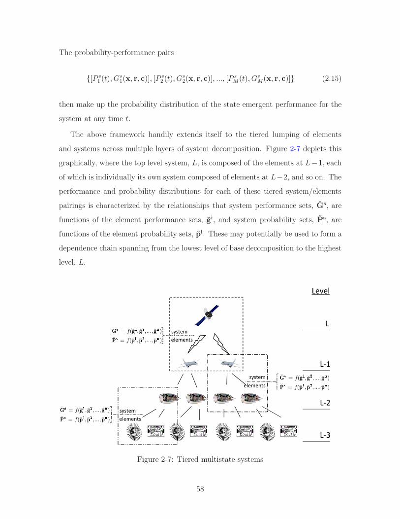
The probability-performance pairs
{[P s1 (t), G
s1(x, r, c)], [P
s2 (t), G
s2(x, r, c)], ..., [P
sM(t), Gs
M(x, r, c)]} (2.15)
then make up the probability distribution of the state emergent performance for the
system at any time t.
The above framework handily extends itself to the tiered lumping of elements
and systems across multiple layers of system decomposition. Figure 2-7 depicts this
graphically, where the top level system, L, is composed of the elements at L−1, each
of which is individually its own system composed of elements at L−2, and so on. The
performance and probability distributions for each of these tiered system/elements
pairings is characterized by the relationships that system performance sets, Gs, are
functions of the element performance sets, gi, and system probability sets, Ps, are
functions of the element probability sets, pi. These may potentially be used to form a
dependence chain spanning from the lowest level of base decomposition to the highest
level, L.
systemelements
elementssystem
systemelements
Level
L
L-1
L-2
L-3
( , ,..., )
( , ,..., )
f
f
=
=
Z [ \ ]Z [ \ ]G g g g
P p p p
�
� � �
�
� � �
( , ,..., )
( , ,..., )
f
f
=
=
^ _ ` a^ _ ` aG g g g
P p p p
�
� � �
�
� � �
( , ,..., )
( , ,..., )
f
f
=
=
^ _ ` a^ _ ` aG g g g
P p p p
�
� � �
�
� � �
Figure 2-7: Tiered multistate systems
58
While conceivable that future improvements in methods and computational ability
will allow the full analysis of multiple system tiers for multiple states, for now this
thesis limits itself to the simultaneous analysis of one system involving potential
failure of one level of subelements. This does not imply that the analysis neglects the
effects of failures at the lowest levels of decomposition. The failure of a component
at level L − 1 may indeed be caused by the failure of a component at level L − 2
or L − 3. As long as the element transition rate (typically 1/MTBF in the case of
failures) corresponds to the proper level of decomposition, how the failure occurs is
irrelevant to the analysis.
2.3.2 Markov Analysis
The preceding section established that the performance of any system may be mod-
eled as a stochastic process, characterized by a set of state performance (Gs) and
probability (Ps) pairings that describes the system’s performance probability distri-
bution at any time t ≥ 0 [69]. The following section describes a process by which one
may efficiently determine the values in Ps, using information about the rates of state
transition of its elements.
In general, a stochastic process is a family of random variables indexed by some
parameter, such as time or space (e.g. Gs = {Gs(t) : t ≥ 0}). The values assumed
by the process vary according to the assignment of these random variables drawn
from a larger set of all possible outcomes [20] (e.g. Gs(t) ∈ Gs). The set of all
possible outcomes comprises the state-space, and, in the case of multistate system
analysis, the index is typically time, t. Both the state-space and time may be classified
as continuous or discrete, giving rise to four categories of stochastic processes. The
category of discrete-state and continuous-time occurs very frequently in the analysis of
multistate failures, given that one can probabilistically predict the transition rates of
system elements, in the continuous-time spectrum, based on historical data regarding
their mean-time-between-failure or mean-time-to-repair. The process with a discrete-
state space is typically called a chain.
Extending nomenclature one step further, under the simplification of Eqn. 2.8,
59

the transition probabilities between elemental states k may be defined as
λi(t,∆t) = Pr{git+∆t = giF |git = giOP} (2.16)
which is the probability that the element is in a state of failure at time, t+∆t, given
that it was in a state of operating at time, t, and
µi(t,∆t) = Pr{git+∆t = giOP |git = giF} (2.17)
which is the probability that the element is in a state of operating at time, t + ∆t,
given that it was in a state of failure at time, t. The above transition rates form the
sets λs = {λ1, λ2, ..., λn} and µs = {µ1, µ2, ..., µn}. If the system states that occur at
time t+∆t as a result of these transitions only depend upon the system state at time
t, the process is said to be Markovian, representable by the well developed theory
first introduced by A. Markov in 1907 [55].
Furthermore, when the transition probabilities do not depend on t, but only ∆t,
the stochastic process is said to be in a steady state and the Markov process is ho-
mogeneous. The respective probabilities λi and µi are then equal to MTBF−1 and
MTTR−1 (mean-time-to-repair), which typically have units [1/hr] and are referred
to as failure rates and repair rates. Figure 2-8 shows a generic representation of the
resulting discrete-state Markov chain, for a three element system without repair (for
an example with repair, see Fig. 2-10). Appropriate nomenclature from the previous
section has been included and the state definitions are given in Table 2.1. In this
formulation, P sK may be interpreted as the probability that the system finds itself
in any particular state of performance GsK at time t. These probabilities may be
determined through Markov analysis as described later in this section via Eqns. 2.18
through 2.24, knowing the transition probabilities λi or µi.
There are some important characteristics of the formulation in Fig. 2-8 that de-
serve note, and help in understanding the general process of constructing Markov
chains (for failure analysis). To begin, the structure of the chain is first determined
by the state definitions, and then by the transition paths. For instance, State 8 is
60
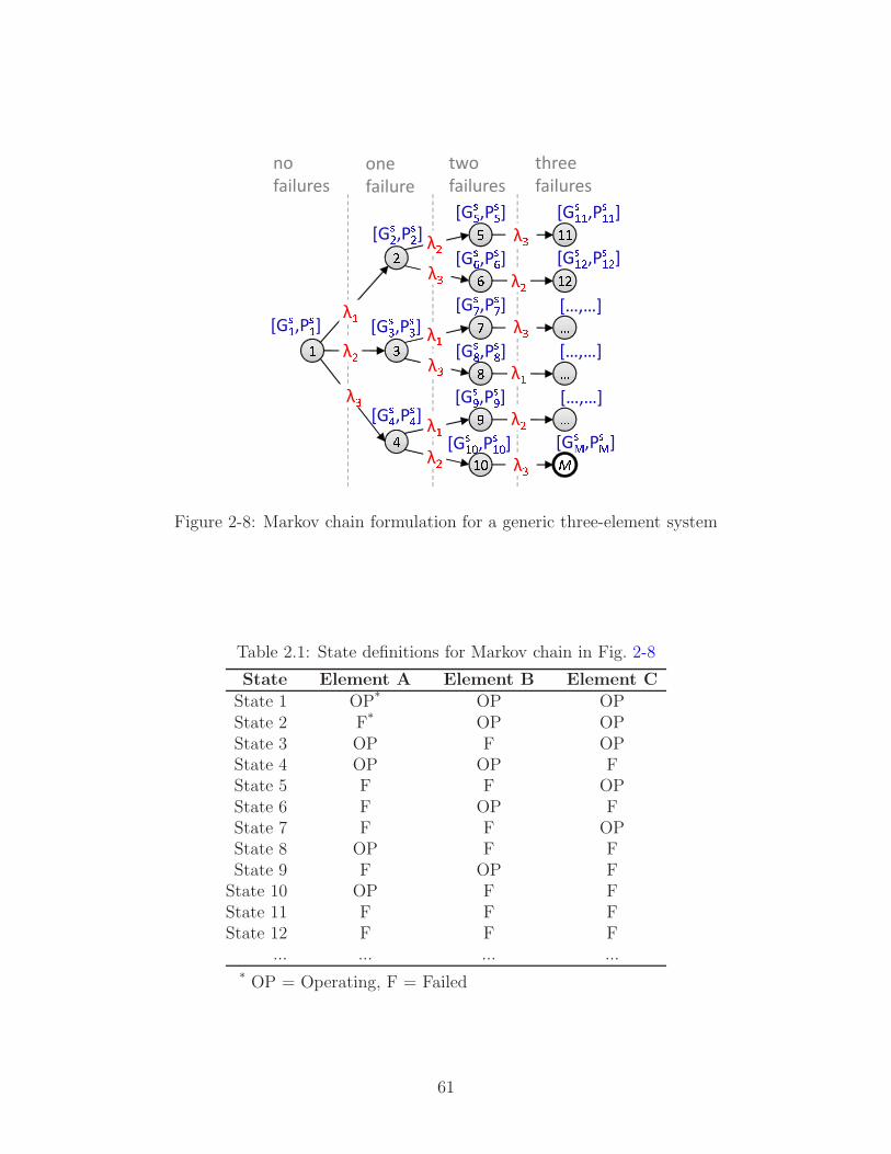
b c def
gh
λiλjλk[Gli,Pli] mn
bgbbooo[…,…]
p
λjλk λjλkλiλq λk
λiλiλj λj
λk […,…]
[Glr,Plr]
[…,…]
[Glj,Plj][Glk,Plk][Gls,Pls] bt
[Glu,Plu][Glv,Plv][Glw,Plw][Glx,Plx][Gly,Ply]
[Gliz,Pliz]
[Glii,Plii][Glij,Plij]
no failures
one failure
two failures
three failures
Figure 2-8: Markov chain formulation for a generic three-element system
Table 2.1: State definitions for Markov chain in Fig. 2-8
State Element A Element B Element C
State 1 OP* OP OPState 2 F* OP OPState 3 OP F OPState 4 OP OP FState 5 F F OPState 6 F OP FState 7 F F OPState 8 OP F FState 9 F OP FState 10 OP F FState 11 F F FState 12 F F F
... ... ... ...* OP = Operating, F = Failed
61

defined by the fact that Elements 2 and 3 are failed, therefore it is located at the two
failures level. In the case of the above depiction, the fact that Element 2 failed before
Element 3 is important, therefore the path to State 8 is State 1→State 3→State 8.
If symmetry is assumed, that is, state performance does not depend on the order in
which the elements have failed, performance in State 8 is the same as in State 10
(Gs10 = Gs
8), and the Markov chain may be recombined as that in Fig. 2-9. In this
case, State 7 takes the place of States 8 and 10 in Fig. 2-8, and is arrived at via paths
State 1→State 3→State 7 OR State 1→State 4→State 7. The probability of being
in a state with both Elements 2 and 3 failed, regardless of path, is exactly the same
for both Fig. 2-8 and Fig. 2-9, with P s7 in Fig. 2-9 equal to the sum of P s
8 and P s10
in Fig. 2-8. It is only the state performances that necessitate the generalization of
Fig. 2-8. The following simple example problem demonstrates the process for solving
a Markov chain for all P sK . Although the example problem is for a simpler chain than
those shown in Figs. 2-8 or 2-9, one easily observes that the advantage of the Fig. 2-9
formulation is a smaller set of equations in the system of ODE’s in Eqn. 2.23.
1 3 6
5
8
7
2
4
λ{λ|λ}
λ}λ} λ}λ{
λ{λ|λ| λ{
λ|[G~{,P~{] [G~|,P~|][G~},P~}][G~�,P~�] [G~�,P~�]
[G~�,P~�][G~�,P~�][G~�,P~�]
no failures
one failure
two failures
three failures
Figure 2-9: Markov chain formulation for a symmetric three-element system (stateperformance is order independent)
Consider the possible failures of two engines, depicted by the Markov formulation
in Fig. 2-10. For generality, cyclic transitions are allowed via repair rates, modeling
62

perhaps a future long-duration air vehicle with on-board diagnostics and possible
in-flight repair. Although both engines may have the same chance of failing, the
performance of the vehicle may be different depending on whether the right or left
engine is operating, thus there are four distinct states of operation.
� �� ��� ���� ���� ��
�� ��Figure 2-10: Markov diagram for two-engine failure scenario with repair
State 1 has both engines operating, while in State 2 only the starboard engine B
is functional and in State 3 only the port engine A is functional. State 4 is the fully
failed state in which both engines are non-functioning. The λi values are the failure
rates of A and B while the repair rates feed transition in the upstream direction. Note
that direct transition from State 1 to State 4 could occur with the exact simultaneous
failure of both engines, but this would in nearly all circumstances be caused by the
failure of a third element somewhere in the system, and is not considered here.3
Beginning with State 1, for a time period [t, t+δt), the probability that the aircraft
leaves State 1 is given by
Pr1→ = λAδt + λBδt = (λA + λB)δt (2.18)
Subsequently, it follows that the probability of being in State 1 at time t + δt is
determined from
P s1 (t + δt) = P s
1 (t)(1− (λA + λB)δt) + P s2 (t)µAδt + P s
3 (t)µBδt (2.19)
3Another possibility is that both engines happen to fail through independent causes at the sameinstant. However, this probability tends to zero at the limit, and all paths to State 4 must passthrough State 2 or State 3 for some, possibly infinitesimally small, period of time.
63

which can be stated as, “the probability that the system is in State 1 at t + δt is
equal to summation of probabilities composed of: 1) the probability that it has not
left State 1, 2) the probability that it has arrived at State 1 from State 2, and 3) the
probability that it has arrived at State 1 from State 3.” The same may be done for
States 2, 3, and 4:
P s2 (t + δt) = P s
2 (t)(1− (µA + λB)δt) + P s1 (t)λAδt + P s
4 (t)µBδt (2.20)
P s3 (t + δt) = P s
3 (t)(1− (λA + µB)δt) + P s1 (t)λBδt+ P s
4 (t)µAδt (2.21)
P s4 (t+ δt) = P s
4 (t)(1− (µA + µB)δt) + P12s(t)λBδt + P s
3 (t)λAδt (2.22)
After differentiating at the limit as δt approaches zero, the above provides the system
of first order linear differential equations
dPs(t)
dt= APs(t) (2.23)
where A is the matrix shown in Eq. 2.24.
A =
−(λA + λB) µA µB 0
λA −(µA + λB) 0 µB
λB 0 −(µB + λA) µA
0 λB λA −(µB + µA)
(2.24)
Whereas twenty years ago the solution to Eq. 2.23 required careful formulation regard-
ing computational efficiency, today many commercial solvers exist capable of rapidly
executing it for hundreds or even thousands of states.
Markov analysis provides an efficient means of stochastically modeling state tran-
sition events that might occur in a large, complex system, without having to perform
a full Monte Carlo analysis of the performance space. It does this by constructing
the system level state probabilities on the basis of the individual element state prob-
abilities. This is attractive because it allows the explicit enumeration of every unique
combination and sequence of possible events regardless of probability. A Monte Carlo
64

analysis, on the other hand, may not find highly improbable event sequences (such
as two simultaneous low-probability failures) without a very large number of simula-
tions. This advantage of the Markov process may sometimes come at the expense of
a large state-space in the Markov model, which may be controlled by truncating the
number of independent events (levels of failure) or by aggregating states.
In practice, combining the Markov model construction of more complex architec-
tures with an integrated system model allows the user to enumerate the dependency
structure of the individual components. This capability ensures that dependent fail-
ures or cascading effects are adequately represented in the performance index esti-
mates, which are not typically captured through other estimation techniques.
2.3.3 Indices of Multistate Performance
If the performance levels GsK(x, r, c) can be determined, and P s
K(λs,µs, t) calculated
from Eqn. 2.23, the system’s expected availability, EA, and expected performance,
EG, arise as indices of multistate performance. These indices, or some form of them,
are integral to the multistate analysis and design methodology developed Chapter 4,
in that they compose the objective functions used to measure the effects of changes to
static design variables, x, and element transition rates, λi and µi, on overall multistate
performance output. They should be considered in contrast to the system’s nominal
performance, defined as the system’s design performance level in the fully operational
state.4
First, consider that over a mission time interval [0,T], some performance threshold
requirement, W , exists that divides the set of system state performances into two cat-
egories of acceptable and unacceptable. The summation of probabilities from the set,
Ps, corresponding to the acceptable category, is a measure of the system’s expected
availability at any time t. For the cases modeled in the remainder of this thesis, the
mission interval itself is the time of interest, therefore t = T and the dependency on
4Note that this definition does not preclude the system from obtaining a level of nominal perfor-mance in a state other than fully operational. As the methodology stresses performance in the faceof degradation, it is only appropriate that it should be possible to maintain a nominal performancerate in an other than fully operational state.
65

time is accounted for implicitly through the probabilities resulting from Eqn. 2.23.
The resulting equation for availability is [67]:
EA =Z∑
z=1
Q(Wz)TzT
where Q(Wz) =∑
GsK≥Wz
P sK (2.25)
Here, T represents the mission interval time, potentially divided into Z intervals of Tz
where each interval may have its own acceptable minimum performance level,Wz. For
cases of constant W , the availability is simply the summation of state probabilities
corresponding to states with performance greater than or equal to W , as shown in
the equation on the right.
Eqn. 2.26 gives the analogous formulation for expected performance,
EG =
M∑
K=1
P sKG
sK (2.26)
which is the summation of each of the state performances, weighted by the probability
that they occur.
2.4 Chapter Summary
The objective of this chapter was to provide an overarching understanding of multi-
state design in the context of complex systems. It began with a detailed review of
literature in multistate design, and placed the thesis work in its proper scope within
an expanded hierarchy of system state change. Next, certain elements of the reviewed
research were used to extend the multistate nomenclature and framework from rela-
tively simple systems to one suitable for analysis of more complex aerospace systems.
Markov analysis was then shown to be an effective method for calculating the state
probabilities required to complete the above analysis. It enables assessment of indi-
vidual state probabilities, performances, and interstate transitions individually, sep-
arately, and concurrently, allowing for computation of the system level probabilities
through Eqn. 2.23, covering all combinations of possibilities. These would otherwise
66
require a very large and expensive Monte Carlo analysis to query the performance
space for the full scope of failure permutations. Finally, two measures of multistate
performance were introduced, system availability and expected performance, which,
although rather basic in form, are very complex functions of many inputs, including
design variables, failure and repair rates, mission duration, and operational parame-
ters.
67

68

Chapter 3
Case Study - I: Twin-Engine
Aircraft
The objective of this chapter is to quantify the effect of changes to a known air-
craft’s static design variables on its performance output for differing aircraft states.
This is accomplished through design sensitivity analysis by evaluating the expected
performance and availability of the system across various time periods and subject
to changes in component or element mean-time-between-failures. The goal is to es-
tablish that such sensitivities exist and can be useful for more detailed performance
evaluation and tradespace exploration with robust, long-endurance system concepts.
The above is accomplished by applying the basic framework laid out in Chapter 2,
extended to more complex aerospace systems, and enabled by the development of a
multi-modal performance model, which is validated through extensive flight test data
collected at Edwards AFB Flight Test Center. It includes elements for determining
responses in aircraft expected performance and availability to changes in 1) static
design variables and 2) component failure rates, accounting for 3) control design vari-
ables (gains) where appropriate, which are the three driving input categories affecting
the aircraft’s performance robustness. The approach is made novel through its inclu-
sion of the functional dependency of each of these variables on the system’s multistate
performance response, and the integration of Markov analysis directly into the early-
stage design loop (a more formal development is given in Chapter 4). Markov chain
69
analysis within the design loop stochastically models the state transitions based on
failure rates, and gain optimization through simulation ensures controllability at each
design point. Results showed unsafe performance in 15% of the aircraft’s geometry-
state responses under investigation. While many occurred in the fully failed state
and were expected, five occurred in partially degraded states where the majority of
geometries were able to meet performance requirements. Furthermore, this behavior
clearly exhibited itself in the resulting design sensitivities, confirming that such an
approach allows designers to identify elements that might drive system loss through
analysis of performance changes across system states and their respective response to
changes in design variables.
The chapter begins with a description of the twin-engine aircraft design model
and the flight test data used for its validation. The second section outlines the
specific approach as applied to the case study, and the final sections present results
of the multistate analysis, including sensitivities of performance metrics to design
variables. More detail on the multi-modal simulation-based design model is provided
in Appendix A and an analysis of reachability for the worst performing states is given
in Appendix B.
3.1 Aircraft Integrated System Model
This section describes development of the multistate design model and techniques
used in evaluating multistate performance. These are the tools necessary for popu-
lating the system state performance set, Gs, to be used along with the probability
set, Ps, in forming the system’s probability distribution of performance.
The design problem for the case under study is divided into an aspect oriented
hierarchy with subdisciplines of mass and inertias, aerodynamic forces and moments,
propulsion, and performance. Fig. 3-1 shows a simplified depiction of the design
structure matrix (DSM) depicting model information flow. All geometry is entered
as basic aircraft design variables such as aspect ratio, taper ratio, wing sweep, fuselage
height and width, engine location, etc., which are used to calculate mass and inertias
70

for the aircraft’s various components. These geometric parameters are also passed to a
preprocessor for input to a vortex lattice code as geometric coordinates for discretized
lifting surface panels. A few of the geometric parameters are handled directly by a
flight simulator executable in the performance module, such as the location of the
fuel tanks, included so that the inertial effects of fuel burn may be directly accounted
for during run-time.
GEOMETRY
Mass & Inertias(Matlab)
Aero Forces & Moments
(AVL �� �������)Propulsion
Performance(JSBSim �� ���)
6-DOF SimulationState Model
BC
A
F
DE
K
G��, G��(t)[S, b, λ, t/c, Λ, Γ, loc.]����� ����� ����A -- [l ¡�, w ¡�, h ¡�, loc ¡�, loc�¢£¤]
[l¢��, d¢��, loc¢��], [Λ������, λ������, %¥¢�¦] B -- A + [S£�§¢¤¨��, S¢§¢�, S¤¡¦, S §£©�][Weight]����� ����� ����� ¡�� ¢��� �¢£¤� ª��«�C -- [l¬¬, I, I®®]����� ����� ����� ¡�� ¢��[x«���, y«���, z«���]����� ����� ����� ¡�� ¢��� �¢£¤� ª��«D – [loc ¡¢§ �£�¯�]{C°vs. α}, {C±vs. α}, [C°² , C°²¢, C±² , C±²¢]E -- [C§³, C§©, C§¤, C§²£, C§²¤], [Cª´, Cªµ, Cª²¢, Cª² ]
[C�³, C�¤, C�²¤, C�²£], [C¶³, C¶©, C¶²¤, C¶²£]F -- [Thrust, TSFC]
· ¸ ¹º»¼½¾¿¾À¾ÁÂÃÄÅÆ¿ÇÈÆ¿É ÊË ·¼··ÌÌÌÄÍÇÍÉÎϾÀ¾ÁÂà ¾À¾ÁÂþ¿¾ÁÐÑ ¾ÁÂþ¿¾¿¾À ¾À¾ÁÂà ÄÍÇÍÉÄÅÆÒÇÈÆÒÉÄÍÇÍÉÄÅÆÀÇÈÆÀÉÄÅÆÃÇÈÆÃÉÄÅÆÓÇÈÆÓÉ ·ÔÄÅÆÕÇÈÆÕÉÄÅÆÖÇÈÆÖÉÄÅÆ×ÇÈÆ×ÉÄÅÆØÇÈÆØÉÄÅÆÙÇÈÆÙÉÄÅÆ¿ÚÇÈÆ¿ÚÉ
ÄÅÆ¿¿ÇÈÆ¿¿ÉÄÅÆ¿ÀÇÈÆ¿ÀÉFigure 3-1: Multistate aircraft design model data flow
The mass and inertias discipline computes various component weights using em-
pirically based equations from Brandt et al. [25] and Roskam [92]. Inertias are then
calculated for each of these components by discretizing them into smaller divisions,
computing the divisional centers of gravity, and summing the discretized inertias to
get Ixx, Iyy, Izz, and Ixz for the wing, tail, fuselage, etc. The remaining products of
inertia, Ixy and Iyz, are not considered, due to the aircraft’s symmetry of mass and ge-
ometry about these axes. Each component value is passed to the aerodynamic forces
and moments module, where total vehicle inertias are computed through the parallel
axis theorem and used to help determine the aircraft’s response characteristics. All
71
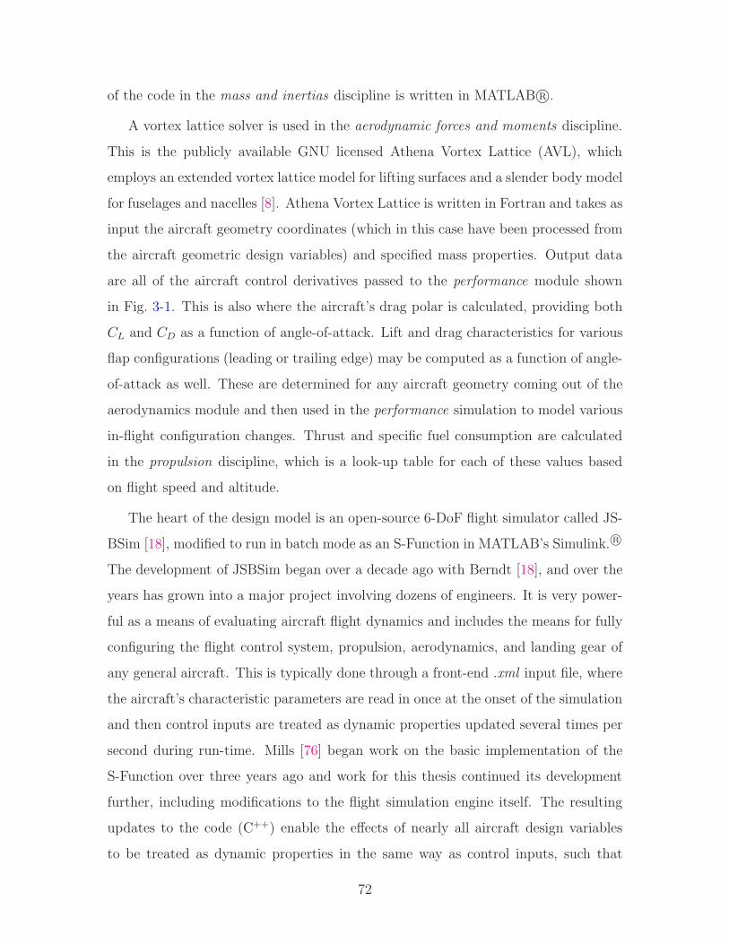
of the code in the mass and inertias discipline is written in MATLAB R©.
A vortex lattice solver is used in the aerodynamic forces and moments discipline.
This is the publicly available GNU licensed Athena Vortex Lattice (AVL), which
employs an extended vortex lattice model for lifting surfaces and a slender body model
for fuselages and nacelles [8]. Athena Vortex Lattice is written in Fortran and takes as
input the aircraft geometry coordinates (which in this case have been processed from
the aircraft geometric design variables) and specified mass properties. Output data
are all of the aircraft control derivatives passed to the performance module shown
in Fig. 3-1. This is also where the aircraft’s drag polar is calculated, providing both
CL and CD as a function of angle-of-attack. Lift and drag characteristics for various
flap configurations (leading or trailing edge) may be computed as a function of angle-
of-attack as well. These are determined for any aircraft geometry coming out of the
aerodynamics module and then used in the performance simulation to model various
in-flight configuration changes. Thrust and specific fuel consumption are calculated
in the propulsion discipline, which is a look-up table for each of these values based
on flight speed and altitude.
The heart of the design model is an open-source 6-DoF flight simulator called JS-
BSim [18], modified to run in batch mode as an S-Function in MATLAB’s Simulink. R©
The development of JSBSim began over a decade ago with Berndt [18], and over the
years has grown into a major project involving dozens of engineers. It is very power-
ful as a means of evaluating aircraft flight dynamics and includes the means for fully
configuring the flight control system, propulsion, aerodynamics, and landing gear of
any general aircraft. This is typically done through a front-end .xml input file, where
the aircraft’s characteristic parameters are read in once at the onset of the simulation
and then control inputs are treated as dynamic properties updated several times per
second during run-time. Mills [76] began work on the basic implementation of the
S-Function over three years ago and work for this thesis continued its development
further, including modifications to the flight simulation engine itself. The resulting
updates to the code (C++) enable the effects of nearly all aircraft design variables
to be treated as dynamic properties in the same way as control inputs, such that
72

they can be varied as a functions of time during the execution of the flight model in
Simulink. This makes possible the rapid evaluation of a wide range of aircraft perfor-
mance parameters for a nearly limitless number of aircraft configurations, including
simulation of failure states, e.g. loss of actuators and engine failures. See Appendix A
for more detail about the simulation model.
3.1.1 Performance Validation
To demonstrate the multistate design problem, the analysis begins with the baseline
configuration of a Beechcraft Super King Air Model 200, as shown in Figs. 3-2 and 3-3.
This aircraft was chosen because its behavior is well understood and there are ample
geometry data which are publicly available [37, 53]. Additionally, the author of this
thesis has numerous flight hours testing the C-12C, which is the Air Force modified
version of the Super King Air to which this particular computational model was
calibrated. The aircraft is powered by two Pratt and Whitney PT6A-41 turboprop
engines, each rated at 850 horsepower (sea level), and is equipped with a rudder
boosted yaw damper system.
Figure 3-2: Super King Air Model 200 3-view (public domain)
Care was taken to ensure that results from the vortex lattice analysis and from
flight simulation were representative of the real-world aircraft. Thus, comparisons
were made to flight test validated data taken from an in-flight performance evaluation
of the Beech C-12C performed at Edwards AFB, CA, in 2001 [106], and raw flight
73
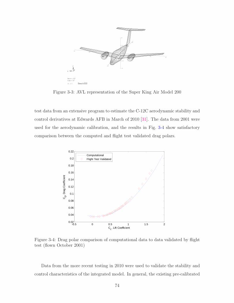
Figure 3-3: AVL representation of the Super King Air Model 200
test data from an extensive program to estimate the C-12C aerodynamic stability and
control derivatives at Edwards AFB in March of 2010 [31]. The data from 2001 were
used for the aerodynamic calibration, and the results in Fig. 3-4 show satisfactory
comparison between the computed and flight test validated drag polars.
-0.5 0 0.5 1 1.5 20.02
0.04
0.06
0.08
0.1
0.12
0.14
0.16
0.18
0.2
0.22
CL, Lift Coefficient
CD,
Dra
g C
oeff
icie
nt
Computational
Flight Test Validated
Figure 3-4: Drag polar comparison of computational data to data validated by flighttest (flown October 2001)
Data from the more recent testing in 2010 were used to validate the stability and
control characteristics of the integrated model. In general, the existing pre-calibrated
74

model arising from the analyses depicted in Fig. 3-1 was quite accurate and only
small adjustments (less than 5% from baseline) were made to the mass estimation
routines and control surface geometries in order to reach the demonstrated results for
angle-of-attack and sideslip shown in Fig. 3-5 and 3-6.
26 28 30 32 34 36 38-8
-6
-4
-2
0
time (sec)
elev
ator
pos
ition
(de
g)
Simulation data
Flight test data (Mar 2010)
26 28 30 32 34 36 38-2
0
2
4
6
8
time (sec)
angl
e of
att
ack
(deg
)
Simulation data
Flight test data (Mar 2010)
AIRCRAFT: Beech C-12CCONFIGURATION: Flaps Up, Gear UpWEIGHT: 10,020 lbsALT: 15,000 ftA/S: 180 KTAS
RMSE = 0.391 deg
Figure 3-5: Comparison of angle-of-attack response
The data depicted in Fig. 3-5 show excellent matching between the computed and
flight test angle-of-attack response to an elevator doublet, with a root-mean-square
error (RMSE) of less than 0.4 degrees. In the yaw-axis, shown in Fig. 3-6, results are
satisfactory in that both response frequencies are the same, although the computed
model shows more damping than the actual aircraft response, resulting in a higher
RMSE of 1.81 degrees. This does not significantly affect the impact of this study’s
results for two reasons. First, a more comprehensive estimate of the aircraft’s yaw-
roll interaction is |Cnβ/Clβ|. As described in the results section of this chapter, the
aircraft model predicts a |Cnβ/Clβ| of 0.38, while that derived from the flight test is
0.35 and comes from data across several flights. Both |Cnβ/Clβ| values are in close
agreement and border the region typically indicative of poorly damped Dutch roll.
Secondly, although the flight-test response implies a less damped Dutch roll mode
75
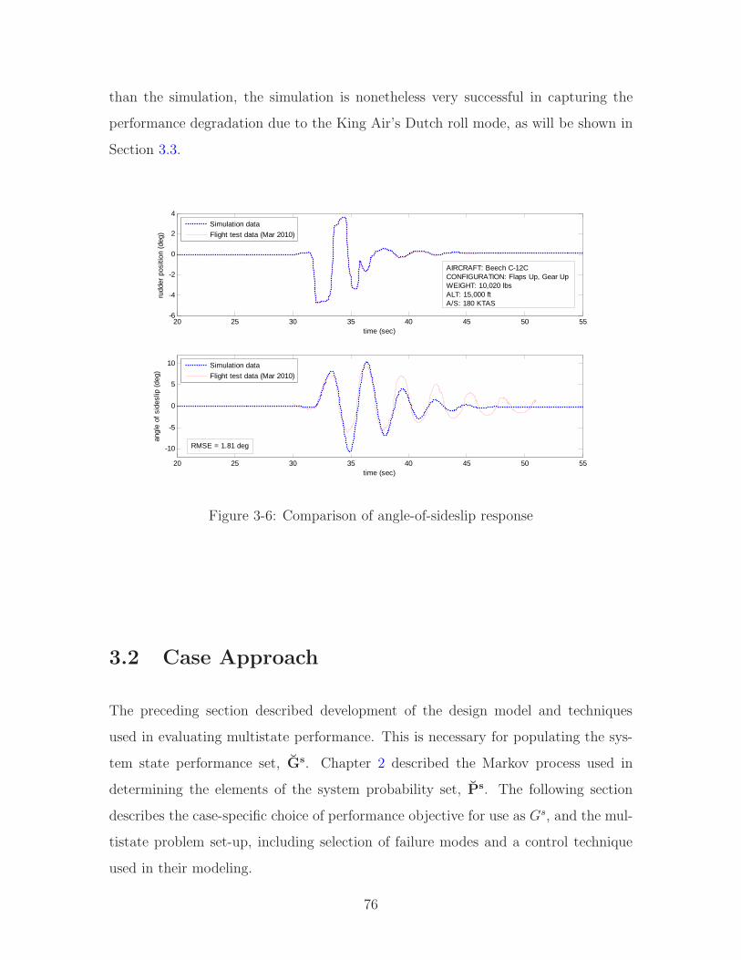
than the simulation, the simulation is nonetheless very successful in capturing the
performance degradation due to the King Air’s Dutch roll mode, as will be shown in
Section 3.3.
20 25 30 35 40 45 50 55-6
-4
-2
0
2
4
time (sec)
rudd
er p
ositi
on (
deg)
Simulation data
Flight test data (Mar 2010)
20 25 30 35 40 45 50 55
-10
-5
0
5
10
time (sec)
angl
e of
sid
eslip
(de
g)
Simulation data
Flight test data (Mar 2010)
AIRCRAFT: Beech C-12CCONFIGURATION: Flaps Up, Gear UpWEIGHT: 10,020 lbsALT: 15,000 ftA/S: 180 KTAS
RMSE = 1.81 deg
Figure 3-6: Comparison of angle-of-sideslip response
3.2 Case Approach
The preceding section described development of the design model and techniques
used in evaluating multistate performance. This is necessary for populating the sys-
tem state performance set, Gs. Chapter 2 described the Markov process used in
determining the elements of the system probability set, Ps. The following section
describes the case-specific choice of performance objective for use as Gs, and the mul-
tistate problem set-up, including selection of failure modes and a control technique
used in their modeling.
76
3.2.1 Design Sensitivity of System Availability and Expected
Performance
While each of the multistate performance metrics (Eqns. 2.25 and 2.26 in Chapter 2)
is useful in its own right, they are even more effective when combined with system
sensitivity analysis. Namely, it is desirable to know how these quantities change as
system variables are modified. This approach has been used in the past for system
reliability analysis [9, 23], using only the component failure rates. In these cases, the
absolute system reliability was of less concern than identifying those elements that
drove the system loss probability. These elements were discovered through sensitivity
analysis, calculating reliability across i number of cases, where each case modified the
failure rate of the ith component. The components that drove system loss were those
that exhibited the largest sensitivity, or change in reliability given a change in λi.
Assuming a single, fixed time period (e.g. Tz = T in Eqn. 2.25), an analogous
sensitivity for EA appears as
dEA(λs,µs)
dλs=
∑
GsK≥W
dP sK(λ
s,µs)
dλs(3.1)
which can, of course, also be shown for the repair rates, µs. The sensitivity in this
case was not necessarily used for direct optimization - it is elementary to know that
reducing a component failure rate will, generally, increase reliability. Rather, it was
used to point the system designers to the portion of the system architecture that had
the greatest effect on reliability. The remedy lied with finding a higher-reliability
component, introducing redundancy, or changing mission parameters.
For the case under study here, system sensitivity analysis is extended to include
effects of static, or geometric, design variables as well. In this way, it is possible not
only to observe sensitivity of availability and expected performance to component
failure rates, but also traditional aircraft design variables, x (wing span, wing area,
engine placement, etc.), or even operational parameters, c (cruise altitude, cruise
speed, etc.). Following the same assumption on time as Eqn. 3.1, this time using
77
expected performance as the example, this takes the form
dEG(λs,µs,x, r, c)
dx=
M∑
K=1
P sK(λ
s,µs)dGs
K(x, r, c)
dx(3.2)
for sensitivity to design variables, x.
Note that by way of the inequality in the summation of Eqn. 3.1, expected avail-
ability becomes a function of x, r, and c as well, although not necessarily a continuous
one. This piecewise constancy does not preclude the local calculation of design sensi-
tivities, but it does pose a problem for gradient-based optimization algorithms. More
will be discussed on this in Chapter 4.
The individual Markov state probabilities P sK in Eqn. 3.2 act as “weights” to
a weighted performance equation. Hence, for short missions, where there is little
chance for the system to enter any but the nominal state, expected performance sen-
sitivity will look much like a standard design sensitivity analysis. However, as system
lifetime or mission duration increases, the probabilities of the off-nominal Markov
states increase and sensitivities may change dramatically. Consider, for example, the
DARPA proposal for an ultra long-endurance UAV with an on-station time of five
years [32]. In this case, expected performance sensitivity is a promising metric for
identifying those system parameters that have the greatest effect on both nominal
and off-nominal system performance, and this analysis may be critical for mission
success.
3.2.2 Aircraft Performance Metrics
The performance function of interest is chosen as expected specific excess power, Ps,1
in a climbing turn, which must be evaluated for the nominal condition and each
of the failure states in order to compute Eqns. 3.1 and 3.2. Ps is computed from
the flight simulation code using the outputs dh/dt, dV/dt, and V in the equation
Ps = dh/dt + (V/g)(dV/dt). The expected performance and availability equations
1Note that P with a subscript s refers to specific excess power, not to be confused with P s, whichrefers to the state probabilities. These are both broadly adopted notations in their respective fields,thus were preserved here despite a slight risk of confusion.
78

resulting from this formulation are given in Eqns. 3.3 and 3.4.
EG(Ps(x),λs) =
M∑
K=1
P sK(λ
s)Ps(x)K =
M∑
K=1
P sK(λ
s)[h(x) +V (x)
gV (x)]avg,K (3.3)
EA(Ps(x),λs) =
∑
[h(x)+V (x)
gV (x)]avg,K≥W
P sK(λ
s) (3.4)
Here, h is altitude, V is velocity, g is the gravity constant, and the avg subscript
indicates the values are averaged over the last ten seconds of the simulation, allowing
the aircraft a chance to stabilize before the performance metric is computed. W
is defined as 200 ft/min for a minimum safe rate of climb (allowing calculation of
Eqn. 3.4), and bank angle must be maintained within ±5◦ to be in the safe region for
calculation of EA(φ(x),λs). Total availability then becomes
EA(Ps(x) ∩ φ(x),λs) =∑
Ps(x)≥200 fpm & φdev(x)≤±5◦
P sK(λ
s) (3.5)
Each simulation was run for a period of sixty seconds (accelerated in batch mode),
beginning from a full-throttle, constant velocity climbing turn at 30◦ of positive bank
(to the right). Initial conditions were set at an altitude of 5000 ft and a velocity
of 140 knots, which is close to the best speed for a cruise climb in the Beech 200.
Engine failure was modeled by cutting the throttle to zero after ten seconds and
control failures disallowed the use of the particular control surface throughout the
simulation, assuming that it was stuck in the neutral position. In the case of engine
failure, the model accounts for additional drag effects of the windmilling engine.
Rather than perform the full re-optimization of an existing aircraft, at this stage
the interest was in identifying those elements that might drive system loss probability
through sensitivity analysis. Therefore, a subset of aircraft geometry variables were
selected and their values perturbed by ±10%, with the exception of wing sweep, which
was varied from 0 to 15 deg. These variables and their values are given in Table 3.1.
Baseline values correspond to those of the aircraft in Fig. 3-2. Note that the values
for the deflecting control surfaces are displayed to the reader as percentages of wing,
79
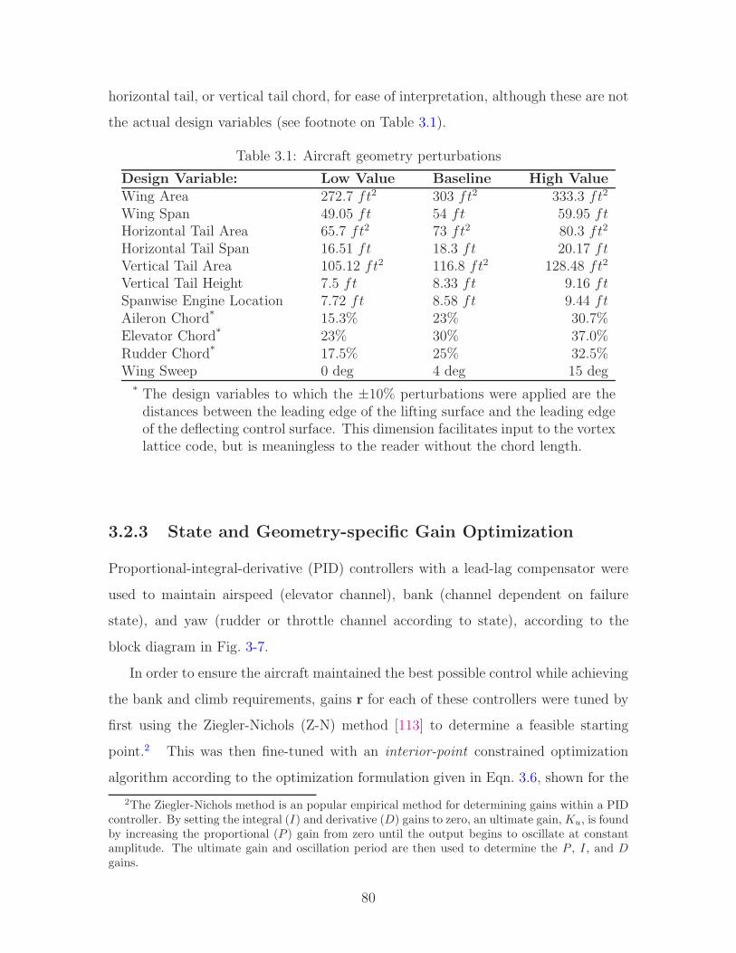
horizontal tail, or vertical tail chord, for ease of interpretation, although these are not
the actual design variables (see footnote on Table 3.1).
Table 3.1: Aircraft geometry perturbations
Design Variable: Low Value Baseline High ValueWing Area 272.7 ft2 303 ft2 333.3 ft2
Wing Span 49.05 ft 54 ft 59.95 ftHorizontal Tail Area 65.7 ft2 73 ft2 80.3 ft2
Horizontal Tail Span 16.51 ft 18.3 ft 20.17 ftVertical Tail Area 105.12 ft2 116.8 ft2 128.48 ft2
Vertical Tail Height 7.5 ft 8.33 ft 9.16 ftSpanwise Engine Location 7.72 ft 8.58 ft 9.44 ftAileron Chord* 15.3% 23% 30.7%Elevator Chord* 23% 30% 37.0%Rudder Chord* 17.5% 25% 32.5%Wing Sweep 0 deg 4 deg 15 deg
* The design variables to which the ±10% perturbations were applied are thedistances between the leading edge of the lifting surface and the leading edgeof the deflecting control surface. This dimension facilitates input to the vortexlattice code, but is meaningless to the reader without the chord length.
3.2.3 State and Geometry-specific Gain Optimization
Proportional-integral-derivative (PID) controllers with a lead-lag compensator were
used to maintain airspeed (elevator channel), bank (channel dependent on failure
state), and yaw (rudder or throttle channel according to state), according to the
block diagram in Fig. 3-7.
In order to ensure the aircraft maintained the best possible control while achieving
the bank and climb requirements, gains r for each of these controllers were tuned by
first using the Ziegler-Nichols (Z-N) method [113] to determine a feasible starting
point.2 This was then fine-tuned with an interior-point constrained optimization
algorithm according to the optimization formulation given in Eqn. 3.6, shown for the
2The Ziegler-Nichols method is an popular empirical method for determining gains within a PIDcontroller. By setting the integral (I) and derivative (D) gains to zero, an ultimate gain, Ku, is foundby increasing the proportional (P ) gain from zero until the output begins to oscillate at constantamplitude. The ultimate gain and oscillation period are then used to determine the P , I, and D
gains.
80
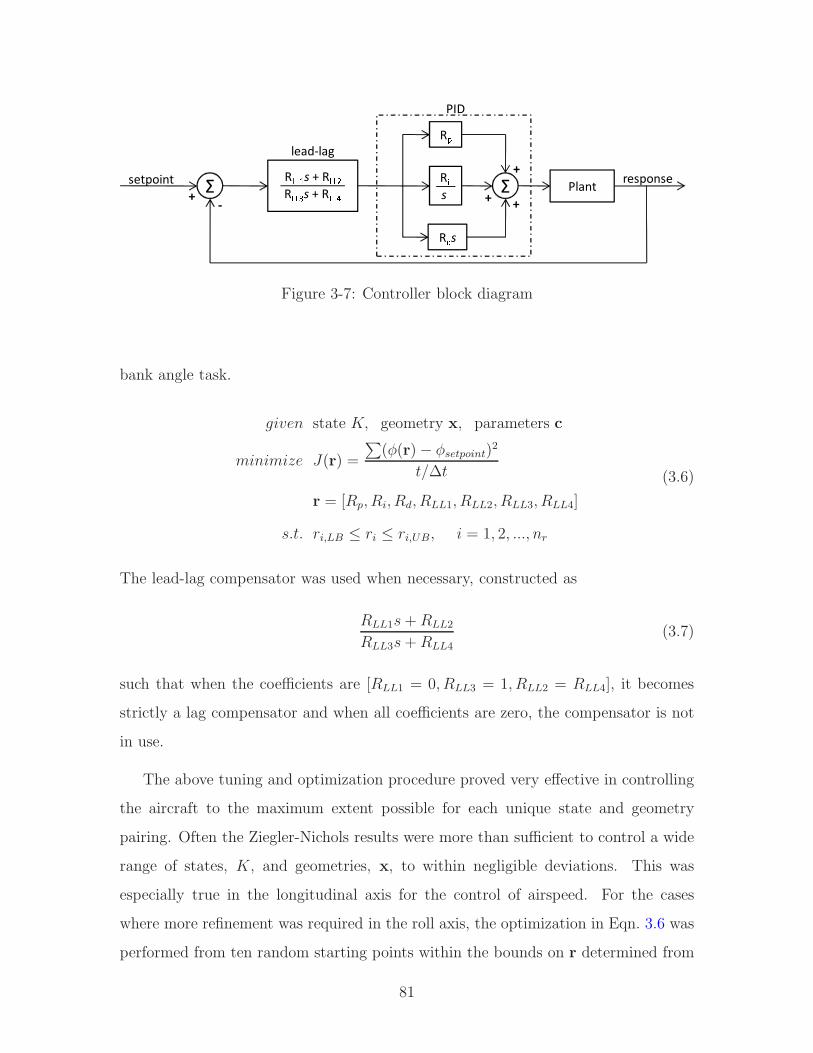
Σsetpoint+
-
RÛÛÜs + RÛÛÝRÛÛÞs + RÛÛßlead-lag
RàRásRâs Σ
+
+ +Plant response
PID
Figure 3-7: Controller block diagram
bank angle task.
given state K, geometry x, parameters c
minimize J(r) =
∑
(φ(r)− φsetpoint)2
t/∆t
r = [Rp, Ri, Rd, RLL1, RLL2, RLL3, RLL4]
s.t. ri,LB ≤ ri ≤ ri,UB, i = 1, 2, ..., nr
(3.6)
The lead-lag compensator was used when necessary, constructed as
RLL1s+RLL2
RLL3s+RLL4(3.7)
such that when the coefficients are [RLL1 = 0, RLL3 = 1, RLL2 = RLL4], it becomes
strictly a lag compensator and when all coefficients are zero, the compensator is not
in use.
The above tuning and optimization procedure proved very effective in controlling
the aircraft to the maximum extent possible for each unique state and geometry
pairing. Often the Ziegler-Nichols results were more than sufficient to control a wide
range of states, K, and geometries, x, to within negligible deviations. This was
especially true in the longitudinal axis for the control of airspeed. For the cases
where more refinement was required in the roll axis, the optimization in Eqn. 3.6 was
performed from ten random starting points within the bounds on r determined from
81

the Z-N results, in order to better search the non-linear design space. If bounds were
reached, they were readjusted and the process reinitialized. The worst performing
cases at the end of the procedure were then analyzed according to their reachability
characteristics as reported in Appendix B.
The optimization approach given in Eqns. 3.6 and 3.7 would not be necessary in
a single state performance analysis. A single state analysis would require only 23
performance simulations to obtain design sensitivities for each of the static design
variables, as opposed to the 184 (23 x 8) required for the full multistate analysis.
The majority (if not all) of these 23 simulations could be controlled by the same set
of controller gains, given the small changes in the system geometry. In the multi-
state case, however, it is extremely time consuming to manually set the gains for
each geometry-state pairing. By allowing each of the gains, as well as the lead-lag
coefficients, to be independent variables in Eqn. 3.6, the optimization can take place
automatically within the design loop, and its results verified at the end of the design
analysis. Such an automated process will be applicable to any system controllable
through PID controllers. In the case of conceptual design, this will likely be suffi-
cient for many types of systems. Where more complex controllers are necessary, more
complex methods will also be required. Fortunately, there is a wide body of research
within controls theory that focuses on such problems (which are beyond the scope of
the research presented here).
3.2.4 State Definition
The previous subsections described the calculation of design sensitivities for the air-
craft’s multistate performance and a means of controlling the system in each of the
states. The determination of which states to include in the analysis is also extremely
important. While the next chapter describes some formal methods to assist in this
determination, in this preliminary examination, failures were limited to those most di-
rectly affecting performance and dynamics, specifically failure of the rudder, ailerons,
and/or a single engine. These correspond to the failure rates λR, λA, and λE , re-
spectively. Typical values of failure rates were used to illustrate effectiveness of the
82

technique at identifying potential issues with the design’s multistate performance,
even given low frequency of failure. Flight control system failure rates were conserva-
tive estimates often used by experts of 1/500000 hrs. Guidance for these values can
be derived from National Transportation and Safety Board (NTSB) data, such as its
Annual Review of Accident Data. For example, 2006 data show that Part 135 air-
plane operations had one accident attributable to flight control system failure over 2.5
million hours of operation [81]. Since the Super King Air is generally a Part 135 on-
demand or scheduled charter aircraft, and not all flight control system failures result
in what the NTSB considers an accident, a 500,000 hour MTBF for the aileron and
rudder control system is a reasonable estimate. Failure rates can vary widely across
aircraft depending on the type of system and/or if software-in-the-loop is used (for
some examples of very poor rates, e.g. 1/5000 hrs in UAVs, see [84]). However, for
purposes of design the direction of performance improvement is much more important
than the absolute magnitude of system availability or expected performance resulting
from a specific combination of failure rates. For the engine, failure rates were set at
8x10⁻⁶ failures per hour, which was then doubled since only the possibility of losing
one engine was considered. Engine failure rates for the Pratt & Whitney PT-6 come
from [36].
If sequence dependence is ignored, the failure of the above elements results in
only eight system configurations to consider, as depicted in the aggregated Markov
model shown in Fig. 3-8. This model appears somewhat different than that shown in
Fig. 2-8 because several of the downstream states can now be reached from multiple
upstream states due to the aggregation. The ODE solution of the model in order to
determine each state probability P sK , however, is performed in the same manner. The
states in the aggregated Markov model are shown in Table 3.2.
Two time periods were used for the analysis of the Markov model and calculation
of state probabilities, P sK . The first was a typical mission duration of 8 hours and the
second was a 20,000-hour time period providing an indication of problem areas that
might manifest themselves over the system lifetime. Results for both time periods
are provided in Section 3.3.
83
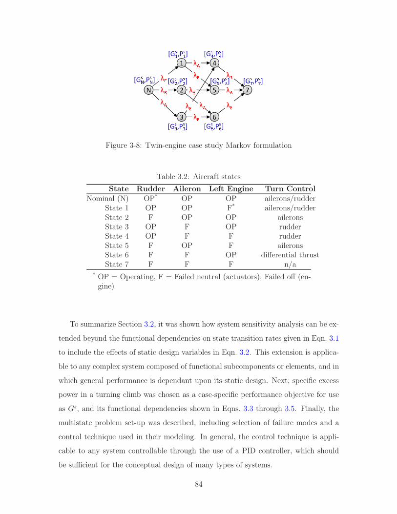
N 2 5
4
7
6
1
3
λãλäλå
λåλå λåλã
λã λäλä λãλä[Gæç,Pæç] [Gæè,Pæè]
[Gæé,Pæé][Gæê,Pæê] [Gæë,Pæë]
[Gæì,Pæì][Gæí,Pæí][Gæî,Pæî]
Figure 3-8: Twin-engine case study Markov formulation
Table 3.2: Aircraft states
State Rudder Aileron Left Engine Turn Control
Nominal (N) OP* OP OP ailerons/rudderState 1 OP OP F* ailerons/rudderState 2 F OP OP aileronsState 3 OP F OP rudderState 4 OP F F rudderState 5 F OP F aileronsState 6 F F OP differential thrustState 7 F F F n/a
* OP = Operating, F = Failed neutral (actuators); Failed off (en-gine)
To summarize Section 3.2, it was shown how system sensitivity analysis can be ex-
tended beyond the functional dependencies on state transition rates given in Eqn. 3.1
to include the effects of static design variables in Eqn. 3.2. This extension is applica-
ble to any complex system composed of functional subcomponents or elements, and in
which general performance is dependant upon its static design. Next, specific excess
power in a turning climb was chosen as a case-specific performance objective for use
as Gs, and its functional dependencies shown in Eqns. 3.3 through 3.5. Finally, the
multistate problem set-up was described, including selection of failure modes and a
control technique used in their modeling. In general, the control technique is appli-
cable to any system controllable through the use of a PID controller, which should
be sufficient for the conceptual design of many types of systems.
84

3.3 Data Analysis
This section presents results of the multistate analysis, including the multistate design
sensitivities with respect to the static design variables. Each geometry in Table 3.1
was run for each Markov state, including one baseline geometry plus 11 low values and
11 high values for a total of 23 geometries. This resulted in 184 simulation runs when
applied to the eight Markov states. Total computational time, not including gain
optimization, was under two minutes on a desktop with an Intel Quad i7 2.8GHz CPU
and 9.0GB of RAM. This time included the benefits of splitting the computations
across eight processing threads, such that the respective Markov states were computed
in parallel.
3.3.1 Multistate Aircraft Performance
To best show the effects of each geometry on the performance metric, the scatter-
plots in Fig. 3-9 were constructed, plotting bank angle vs. specific excess power for
each state. Each plot contains 23 geometries, with the baseline geometry marked by
dashed lines. Note that several geometries may overlap, thus not all 23 instances
are discernible on each plot. The safe region is defined in each plot by a rectangle
bounded by the W limits of ≥ 200 ft/min for Ps and within ±5◦ of the commanded
bank angle of 30◦ as defined previously in Section 3.2. Geometries within the safe
region are considered operational for the particular failure sequence, whereas those
outside of this region will not allow safe completion of the mission. This informa-
tion is used when classifying the performance of a particular Markov state for the
calculation of the expected availability as per Eqn. 3.5.
Of the 184 simulation cases (23 geometries x 8 states), 28 did not achieve safe
performance as established by theW criterion on climb rate and bank angle. Twenty-
three of these resulted in total loss of aircraft and came from State 7, which was to be
expected since there was no way to control the aircraft without use of rudder, aileron,
or differential thrust. Four unsatisfactory cases came from the analysis of State 4,
where the left engine and ailerons were failed, requiring bank angle and turn to be
85
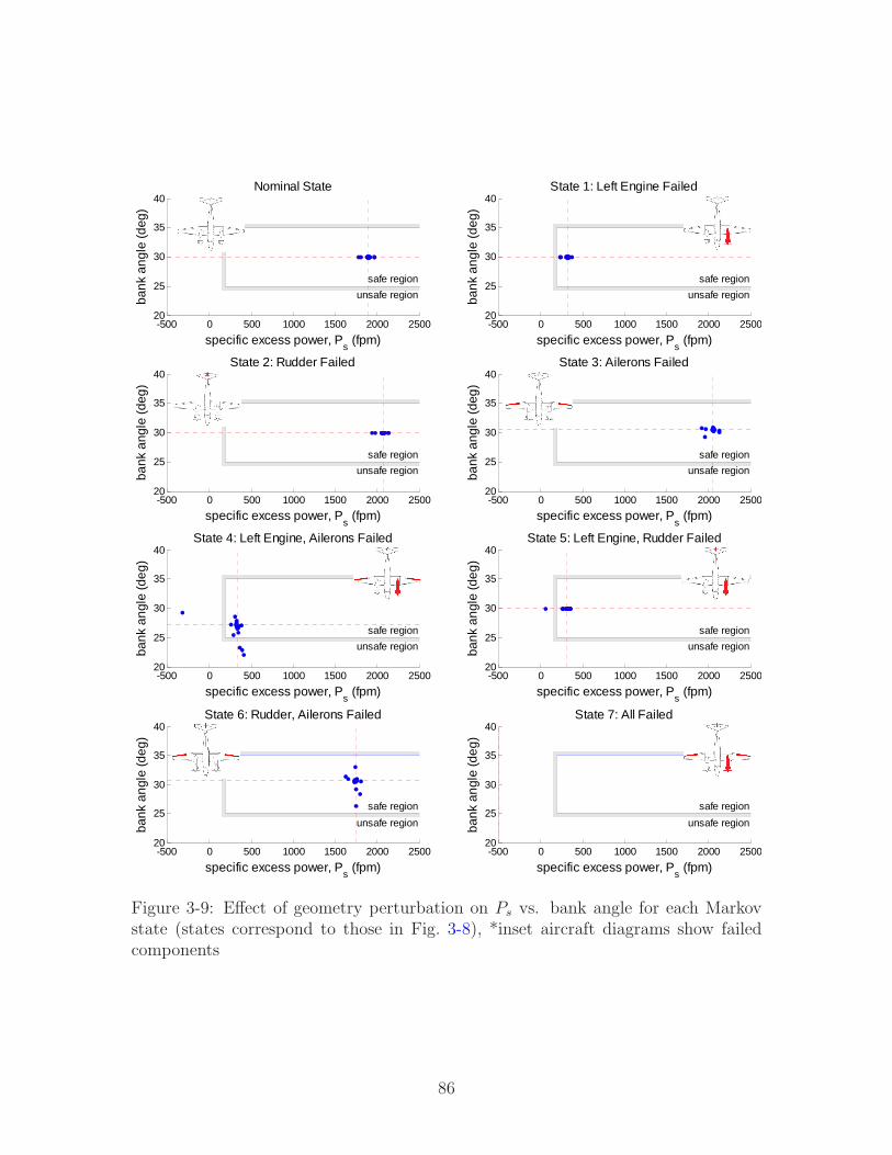
-500 0 500 1000 1500 2000 250020
25
30
35
40
specific excess power, Ps (fpm)
bank
ang
le (d
eg)
Nominal State
unsafe region
safe region
-500 0 500 1000 1500 2000 250020
25
30
35
40
specific excess power, Ps (fpm)
bank
ang
le (d
eg)
State 1: Left Engine Failed
unsafe region
safe region
-500 0 500 1000 1500 2000 250020
25
30
35
40
specific excess power, Ps (fpm)
bank
ang
le (d
eg)
State 2: Rudder Failed
unsafe region
safe region
-500 0 500 1000 1500 2000 250020
25
30
35
40
specific excess power, Ps (fpm)
bank
ang
le (d
eg)
State 3: Ailerons Failed
unsafe region
safe region
-500 0 500 1000 1500 2000 250020
25
30
35
40
specific excess power, Ps (fpm)
bank
ang
le (d
eg)
State 4: Left Engine, Ailerons Failed
unsafe region
safe region
-500 0 500 1000 1500 2000 250020
25
30
35
40
specific excess power, Ps (fpm)
bank
ang
le (d
eg)
State 5: Left Engine, Rudder Failed
unsafe region
safe region
-500 0 500 1000 1500 2000 250020
25
30
35
40
specific excess power, Ps (fpm)
bank
ang
le (d
eg)
State 6: Rudder, Ailerons Failed
unsafe region
safe region
-500 0 500 1000 1500 2000 250020
25
30
35
40
specific excess power, Ps (fpm)
bank
ang
le (d
eg)
State 7: All Failed
unsafe region
safe region
Figure 3-9: Effect of geometry perturbation on Ps vs. bank angle for each Markovstate (states correspond to those in Fig. 3-8), *inset aircraft diagrams show failedcomponents
86
controlled with only the rudder in the face of asymmetric thrust. The remaining case
came from State 5, with the left engine and rudder failed and bank angle controlled
with ailerons.
The most critical failing geometries of State 4 were those with the vertical tail
height decreased by 10% and the spanwise engine location at the greatest distance
from the fuselage. The short tail height was also the failing geometry of State 5.
Experimentation with the control scenarios for this state, as well as numerous hours
of flight testing actual Beech 200 aircraft, motivated suspicion that an unsatisfactory
Dutch roll mode might be to blame. Indeed, inspection of the control derivatives
showed that these two geometries had the lowest values for |Cnβ/Clβ| of all 23 cases.
A general rule in aircraft design is that |Cnβ/Clβ|, which is a measure of the aircraft’s
directional stability in relation to its lateral stability, should be greater than 0.33 for
satisfactory Dutch roll [25]. For the case with the reduced tail height, this value was
0.19 and for the outboard engine placement it was 0.31.
There are a few items to note concerning this finding. First, the design model pre-
dicted a |Cnβ/Clβ| of 0.38 for the baseline aircraft and data collected from the flight
testing in March 2010 [31] indicated a value somewhat less than this but within the
margin of error. Both of these values are very close to the 0.33 threshold and become
more critical at higher angles of attack, as less of the tail is in undisturbed flow. This
is a known characteristic of the Beech 200 and one of the reasons why the aircraft
is equipped with a yaw damper (the yaw damper is only certified for nominal oper-
ation and is shut off in failure conditions, per flight manual emergency procedures).
Second, in five of the eight states, these poor Dutch roll characteristics did not result
in a loss of the aircraft. However, in the adverse circumstances presented by State 4,
the rudder was unable to dampen the Dutch roll mode while also being required to
control bank angle in a turning climb. While it may be argued that this particular
outcome is specific to the scenario and optimum control laws presented here, it does
demonstrate the emergence of critically negative behavior in off-nominal conditions
that can be affected by relatively small changes in geometric design variables. Specif-
ically, a slightly more effective vertical tail would have been helpful in supporting
87
both simultaneous functions; controlling the Dutch roll mode, and maintaining bank
angle.
Finally, regarding engine placement, in some cases intuition might be correct
in suggesting further outboard engine location is desirable for better turn control
through differential thrust. However, results show that the effect of this placement
on inertial and mass properties should not be overlooked, especially when certain
stability characteristics lie on the margin as in the case of State 4.
3.3.2 Design Sensitivities
The determination of which parameters have the greatest effect on overall system
performance and availability is very important. As mentioned earlier, the expected
performance in Eqn. 3.2 tends to treat the Markov state probabilities as “weights.”
Thus, given sufficiently low failure rates, a short Markov time period will have ex-
pected performance values nearly identical to the nominal state. As overall system
lifetime increases, or mission duration in the case of long-endurance vehicles, the
expected system performance will change as off-nominal probabilities increase. To
illustrate this, consider an 8-hour mission and a 20,000-hour system lifetime, both
typical for this type of aircraft. If no repairs are made, the Markov state probabili-
ties will be as those depicted in Table 3.3, given the failure rates mentioned earlier.
Even if repairs are considered, these values provide some indication of the amount
of resources that must be allocated towards maintenance. The third column in Ta-
ble 3.3 is not necessarily applicable to this aircraft, but is included to emphasize the
impact of this analysis on systems expected to operate for long periods of time in
austere environments, for instance an ultra long-endurance unmanned vehicle with a
continuous mission duration of months or years.
Given these probabilities, it is possible to determine the expected system perfor-
mance and availability. More importantly, one may solve the expected performance
sensitivity for the 8-hour sortie, 20,000-hour system lifetime, or 5-year case, or like-
wise observe changes in expected availability. The design variable sensitivities are
perturbations from the baseline geometry, figured from a central difference on the
88
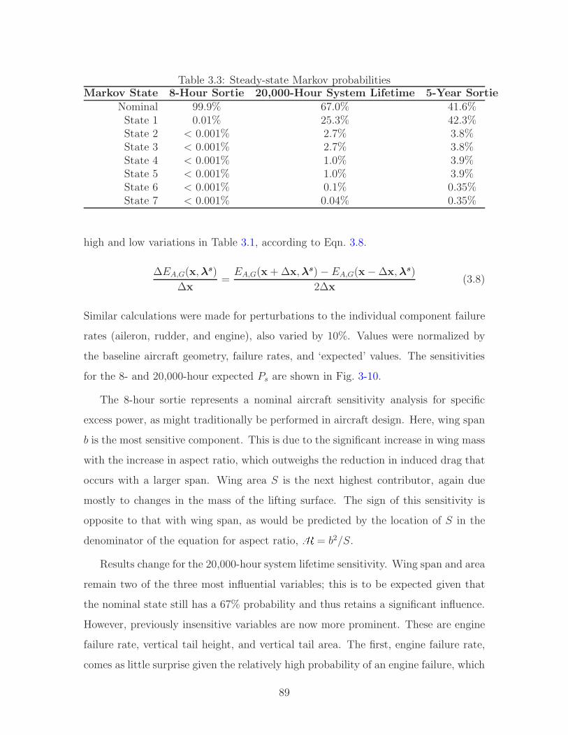
Table 3.3: Steady-state Markov probabilitiesMarkov State 8-Hour Sortie 20,000-Hour System Lifetime 5-Year Sortie
Nominal 99.9% 67.0% 41.6%State 1 0.01% 25.3% 42.3%State 2 < 0.001% 2.7% 3.8%State 3 < 0.001% 2.7% 3.8%State 4 < 0.001% 1.0% 3.9%State 5 < 0.001% 1.0% 3.9%State 6 < 0.001% 0.1% 0.35%State 7 < 0.001% 0.04% 0.35%
high and low variations in Table 3.1, according to Eqn. 3.8.
∆EA,G(x,λs)
∆x=EA,G(x +∆x,λs)− EA,G(x−∆x,λs)
2∆x(3.8)
Similar calculations were made for perturbations to the individual component failure
rates (aileron, rudder, and engine), also varied by 10%. Values were normalized by
the baseline aircraft geometry, failure rates, and ‘expected’ values. The sensitivities
for the 8- and 20,000-hour expected Ps are shown in Fig. 3-10.
The 8-hour sortie represents a nominal aircraft sensitivity analysis for specific
excess power, as might traditionally be performed in aircraft design. Here, wing span
b is the most sensitive component. This is due to the significant increase in wing mass
with the increase in aspect ratio, which outweighs the reduction in induced drag that
occurs with a larger span. Wing area S is the next highest contributor, again due
mostly to changes in the mass of the lifting surface. The sign of this sensitivity is
opposite to that with wing span, as would be predicted by the location of S in the
denominator of the equation for aspect ratio,A = b2/S.
Results change for the 20,000-hour system lifetime sensitivity. Wing span and area
remain two of the three most influential variables; this is to be expected given that
the nominal state still has a 67% probability and thus retains a significant influence.
However, previously insensitive variables are now more prominent. These are engine
failure rate, vertical tail height, and vertical tail area. The first, engine failure rate,
comes as little surprise given the relatively high probability of an engine failure, which
89
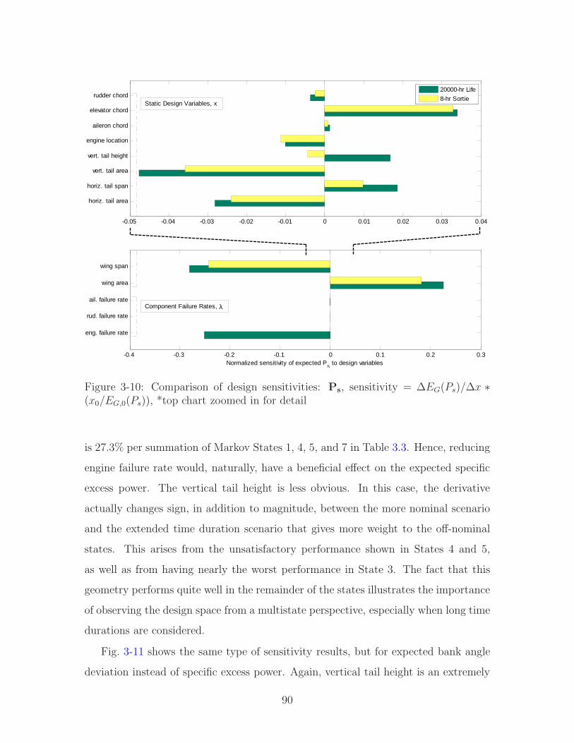
-0.05 -0.04 -0.03 -0.02 -0.01 0 0.01 0.02 0.03 0.04
horiz. tail area
horiz. tail span
vert. tail area
vert. tail height
engine location
aileron chord
elevator chord
rudder chord
20000-hr Life
8-hr Sortie
-0.4 -0.3 -0.2 -0.1 0 0.1 0.2 0.3
eng. failure rate
rud. failure rate
ail. failure rate
wing area
wing span
Normalized sensitivity of expected Ps to design variables
Static Design Variables, x
Component Failure Rates, λ
Figure 3-10: Comparison of design sensitivities: Ps, sensitivity = ∆EG(Ps)/∆x ∗(x0/EG,0(Ps)), *top chart zoomed in for detail
is 27.3% per summation of Markov States 1, 4, 5, and 7 in Table 3.3. Hence, reducing
engine failure rate would, naturally, have a beneficial effect on the expected specific
excess power. The vertical tail height is less obvious. In this case, the derivative
actually changes sign, in addition to magnitude, between the more nominal scenario
and the extended time duration scenario that gives more weight to the off-nominal
states. This arises from the unsatisfactory performance shown in States 4 and 5,
as well as from having nearly the worst performance in State 3. The fact that this
geometry performs quite well in the remainder of the states illustrates the importance
of observing the design space from a multistate perspective, especially when long time
durations are considered.
Fig. 3-11 shows the same type of sensitivity results, but for expected bank angle
deviation instead of specific excess power. Again, vertical tail height is an extremely
90

-5 -4 -3 -2 -1 0 1 2
eng. failure rate
rud. failure rate
ail. failure rate
wing area
wing span
horiz. tail area
horiz. tail span
vert. tail area
vert. tail height
engine location
aileron chord
elevator chord
rudder chord
Normalized sensitivity of bank angle deviation (RMSE) to design variables
20000-hr Life
8-hr SortieStatic Design Variables, x
Component Failure Rates, λ
Figure 3-11: Comparison of design sensitivities: φdev, sensitivity = ∆EG(φdev)/∆x ∗(x0/EG,0(φdev))
important factor in the 20,000-hour scenario, while relatively benign in the 8-hour
sortie. In addition, several sensitivities such as wing span, engine location, and eleva-
tor chord change in both sign and magnitude. Note that sensitivity to engine failure
rate is much less significant in comparison to the other failure rates than in Fig. 3-10.
This is due to the fact that a significant portion of bank angle deviation occurs in
States 3 and 6, in which the engine has not failed.
Finally, the data in Fig. 3-12 demonstrate how changes in design variables and
component failure rates affect the system availability. The driving factors are those
pointed out previously in the analysis of the scatterplots in Fig. 3-9. Although the
engine has the highest component failure rate, its effect on expected availability is
less than the other two components since the failure rate sensitivities were performed
from the baseline geometry, which only has unsatisfactory performance in State 7.
The distribution of probabilities across Markov states for this geometry is such that
changes to aileron and rudder failure rates actually increase the weighting of State 7
more than do changes to the engine failure rate. Only the 20,000-hr and 5-yr results
91

-0.1 -0.05 0 0.05 0.1 0.15 0.2
eng. failure rate
rud. failure rate
ail. failure rate
wing area
wing span
horiz. tail area
horiz. tail span
vert. tail area
vert. tail height
engine location
aileron chord
elevator chord
rudder chord
Normalized sensitivity of expected availability to design variables
5-yr
20000-hrStatic Design Variables, x
Component Failure Rates, λ
Figure 3-12: Comparison of design sensitivities: EA, sensitivity = ∆EA(Ps, φ)/∆x ∗(x0/EA,0(Ps, φ))
are shown, as those for the 8-hr duration are insignificant in magnitude.
The sensitivity results in Fig. 3-12 are compelling, in that they show that improve-
ments to the system’s availability are much more effectively gained through changes
in static design variables than through changes in component failure rate. This is
important, from the perspective of reliability analysis, because improvements in reli-
ability are nearly always sought after in the space of λs rather than affecting through
changes to static design variables, x.
3.4 Case Summary
As mentioned, the objective of this chapter was to quantify the effect of changes to a
known aircraft’s static design variables on its performance output for differing aircraft
states. This was successfully accomplished through design sensitivity analysis by eval-
uating the expected performance and availability of the system across various time
periods and subject to changes in static design variables and component failure rates.
92
Such analysis differs from traditional early-stage design methods, which concentrate
on the system in its nominal state of operation, only infrequently considering failure
states through piecemeal application of constraints. Results from this chapter sug-
gest a weakness in the traditional methodology, showing how small changes in static
design variables may improve performance in the nominal condition, while hurting
performance in off-nominal conditions, resulting in decreased expected performance
or availability across system lifetime or long mission durations. The analysis in this
chapter also differs from reliability analysis, which focuses solely on component failure
rates and the benefits of redundancy but does not consider how well or poorly the
system performs with partial failures. Again, results suggest a weakness with this
approach, showing that in many cases, improvements to the system’s availability or
expected performance are more effectively gained through changes in static design
variables than through changes in component failure rate.
Specifically, results from the Super King Air analysis showed that of 184 geometry
cases, 28 did not achieve satisfactory performance. Many occurred in the fully failed
state and were expected, but several occurred in partially degraded states in which
the majority of geometry cases were able to meet performance requirements. More
importantly, this behavior clearly exhibited itself in the resulting design sensitivities,
confirming that such an approach will allow designers to identify those elements that
might drive system loss probability through an analysis of performance changes across
system states and their respective response to changes in design variables. The results
provide promising evidence as to the utility of expected performance and system
availability analysis applied to a complex aircraft system, and its ability to provide
design engineers with data to generate more robust solutions early in the design
process.
As a final note on the Super King Air application study, development of the
model and stochastic analysis techniques required to obtain the above results high-
lighted two areas for specific attention regarding multistate design. The first is that,
even though the direct effects of multistate analysis are best realized in longer time
duration systems, the benefits of the analysis should be probabilistically observable
93
over operational lifetimes of shorter duration systems as well. The second item is
that the piecewise constant function of system availability will pose great difficulty
for gradient-based optimization algorithms. Chapter 4 addresses both of these issues,
within the context of a formalized multistate analysis and design methodology.
94

Chapter 4
Methodology and Tools for
Multistate Analysis and Design
This chapter proceeds in developing a generalized methodology for multistate anal-
ysis and design, based upon its effectiveness as demonstrated in Chapter 3. The
chapter encompasses three main sections. The first section lays out a methodology
for multistate analysis and design as may be applied to early-stage development of
complex aerospace systems. The second section focuses in on one aspect of that
methodology and develops a multilayer Markov analysis technique enabling transla-
tion of single sortie component and vehicle level availability into metrics for a multiple
sortie mission campaign. Finally, the third section discusses multistate optimization,
specifically, the case of system availability, essentially a piecewise constant function
in which improvement corresponds directly to increasing performance in off-nominal
states above a certain threshold.
4.1 Multistate Analysis and Design
Consideration of the multistate problem is proposed at the earliest stages of the design
process in Fig. 4-1, beginning with requirements and concept development. Next is
an analysis of failure modes, an exercise typically taking place much later in the
design cycle. It is moved forward here in order to provide a vector of transition rates
95
used later in the early phase integrated Markov analysis. The third step classifies
the system according to the performance metric of interest and the nature of its
mission, followed by computational analysis, where analysis of a point design, design
of experiments, or optimization may be exercised. Finally, analysis and visualization
of results are performed as the last step, before deciding whether to iterate again
upon an updated architecture or transition rate vector.
4.1.1 Step 1: Requirements Definition and Concept of Op-
erations
Defining requirements and a concept of operations should occur near the beginning
of any design process and there are many sources describing activity here [38, 82]. To
summarize from the NASA Systems Engineering Handbook [78], it should “transform
stakeholder expectations into a definition of the problem” and should output clear
measures of performance against which the design may be validated.
The step is included here for completeness and to underscore the fact that ad-
ditional considerations must be made for systems designed under the multistate
paradigm. These include, for example:
• Establishment of criteria for the acceptable performance threshold, W .
• Setting of realistic requirements for system availability and/or expected perfor-
mance.
• Determination of how the system will be operated in off-nominal states.
• Establishment of a range of acceptable operational parameters, c.
The importance of the above may vary from system to system, depending on
its nature. Regarding the establishment of criteria for W , it is not sufficient to
merely define unacceptable performance as that resulting in loss of the system. Many
criteria exist whereby the operator would choose to abort the mission even though
the system was still capable of safely operating. This may be directly related to the
value of GsK itself or to the resulting operational conditions arising from that value.
96
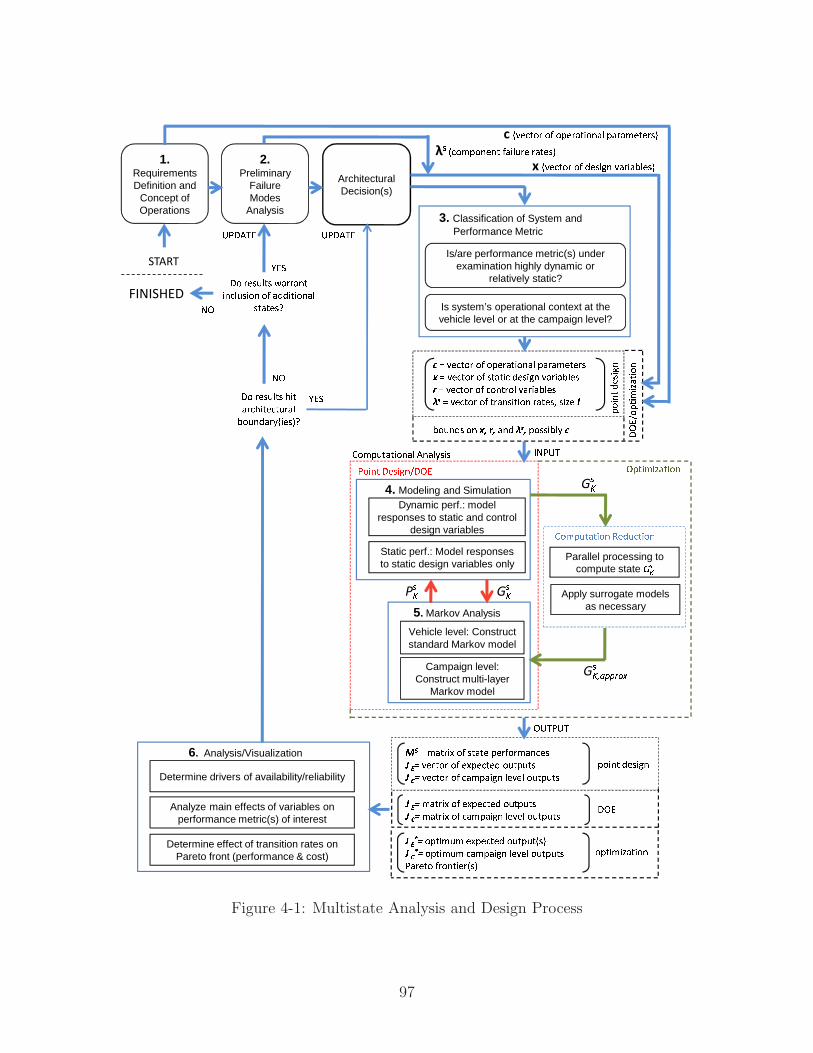
START
1. Requirements Definition and
Concept of Operations
2.Preliminary
Failure Modes
Analysis
Architectural Decision(s)
ï ð ñòóôõö õ÷ õøòöùôúõûùü øùöùýòôòöþÿ ð ñòóôõö õ÷ þôùôúó �òþú�û ñùöúù�üòþ� ð ñòóôõö õ÷ óõûôöõü ñùöúù�üòþ�� ð ñòóôõö õ÷ ôöùûþúôúõû öùôòþ� þú�ò � �� ������ ���� ����� ���õ�û�þ õûÿ� �� ùû���� øõþþú�ü� ï
Vehicle level: Construct standard Markov model
Campaign level: Construct multi-layer
Markov model
Static perf.: Model responses to static design variables only
Dynamic perf.: model responses to static and control
design variables
4. Modeling and Simulation
5. Markov Analysis
�õýø�ôùôúõû �ò��óôúõûParallel processing to
compute state �� Apply surrogate models
as necessaryG
!"#øôúýú�ùôúõû
$% ð ýùôöú& õ÷ þôùôò øòö÷õöýùûóòþ' () ñòóôõö õ÷ ò&øòóôò� õ�ôø�ôþ' *) ñòóôõö õ÷ óùýøùú�û üòñòü õ�ôø�ôþ' (+) õøôúý�ý ò&øòóôò� õ�ôø�ô,þ-' *+) õøôúý�ý óùýøùú�û üòñòü õ�ôø�ôþ.ùöòôõ ÷öõûôúòö,þ-øõúûô �òþú�ûõøôúýú�ùôúõû' () ýùôöú& õ÷ ò&øòóôò� õ�ôø�ôþ' *) ýùôöú& õ÷ óùýøùú�û üòñòü õ�ôø�ôþ /#0Determine drivers of availability/reliability
6. Analysis/Visualization
Analyze main effects of variables on performance metric(s) of interest
Determine effect of transition rates on Pareto front (performance & cost)
.õúûô /òþú�û1/#0�õýø�ôùôúõûùü2ûùü�þúþ
3. Classification of System and Performance Metric
Is system’s operational context at the vehicle level or at the campaign level?
Is/are performance metric(s) under examination highly dynamic or
relatively static?
/õ öòþ�üôþ 3úôùöó3úôòóô�öùü�õ�û�ùö�,úòþ-4/õ öòþ�üôþ5ùööùûôúûóü�þúõû õ÷ ù��úôúõûùüþôùôòþ4FINISHED 6# 708
6# 7089./2:0
;6.9:
#9:.9:P
!"G
!"
G!"<=>>?@A
9./2:0c ,ñòóôõö õ÷ õøòöùôúõûùü øùöùýòôòöþ-
x ,ñòóôõö õ÷ �òþú�û ñùöúù�üòþ-λB ,óõýøõûòûô ÷ùúü�öò öùôòþ-
Figure 4-1: Multistate Analysis and Design Process
97
For example, a failure within a UAV system may result in a loss of endurance, but
minimizing this loss may require increasing or decreasing the cruise altitude by several
thousand feet. Consequently, it will be important to determine the range of flexibility
in mission parameters, typically in the form of operational parameters, c, as part of
the requirements definition.
4.1.2 Step 2: Preliminary Analysis of Failure Modes
The most common form of failure mode analysis is formally referred to as Failure Mode
and Effect Analysis (FMEA), the purpose of which is to “study the results or effects
of item failure on system operation and to classify each potential failure according to
its severity” [35]. It is widely used throughout industry and the originating military
standard (MIL-STD-1629A) is a 54-page document describing a process which may
be succinctly summarized as:
1. Describe the system elements.
2. Determine their function(s).
3. Identify their failure mode(s).
4. Identify the potential cause(s) and effect(s) of the failure.
5. Describe proper corrective action.
6. Classify the failure(s) according to severity.
The FMEA is typically performed after the static design is set. This allows more
detailed analysis of failure effects, but generally limits corrective action to improving
element failure rates or restricting the operational envelope. There are some failures
to which this later stage analysis is best suited. However, effects of many failures can
be accurately predicted much earlier in the design cycle. Integrating a preliminary
FMEA into the early-phase design loop as in Fig. 4-1 has the purpose of 1) identifying
these types of failures, 2) determining their estimated rate of occurrence, and 3) rank
ordering them according to their occurrence rate and effect on performance.
Much of the analysis at this early stage will be based on the designer’s experience
and any historical data that may be available, especially concerning the rates of
98

failure. The most important output of this step is the vector of transition rates,
λs, that will eventually be used as input to the computational analysis. As was
discussed in Chapter 2, the probabilities, P sK , resulting from the Markov analysis, act
as weights in the multistate performance indices. Thus, the more highly probable
and highly consequential failures that are represented in the transition rate vector,
the better. Depending on results of the initial performance and Markov analysis, the
failure modes analysis may be iteratively updated to include more or less states, or
to reorder the failure mode ranking.
4.1.3 Step 3: System and Performance Classification
The classification of the system and its performance metric is necessary in determin-
ing the type of analysis to be performed as part of Step 4 and Step 5. Whether that
analysis is dynamic or static depends upon the level of fidelity sought and the kine-
matic nature of the metric. With metrics such as range or endurance, the effects of
shorter time duration kinematics are generally negligible compared to the cumulative
effects of motive resistance (drag), propulsive forces, and energy consumption. Thus,
a static analysis is possible through physics-based analytic equations that assume
the system is dynamically controllable. Such analyses are common at the conceptual
design level and will be relatively accurate, assuming one can integrate the effects of
failure states into the analysis. On the other hand, if higher fidelity is sought in a
shorter time duration maneuver, such as that of the turning climb in Chapter 3, the
analysis is dynamic and the effects of controllability may be accounted for through
simulation. The primary difference between the two is that one directly includes the
effects of control variables, r, in the analysis and the other assumes the best case
scenario of a fully controllable system. This involves a trade-off between fidelity of
analysis and computational time.
The second categorization under this step has to do with the system’s operational
context and will determine the depth of Markov analysis performed in Step 5. If the
system will only be considered in the context of its own singular operation (vehicle
level), the Markov analysis as described in Section 2.3.2 of Chapter 3 is applicable
99
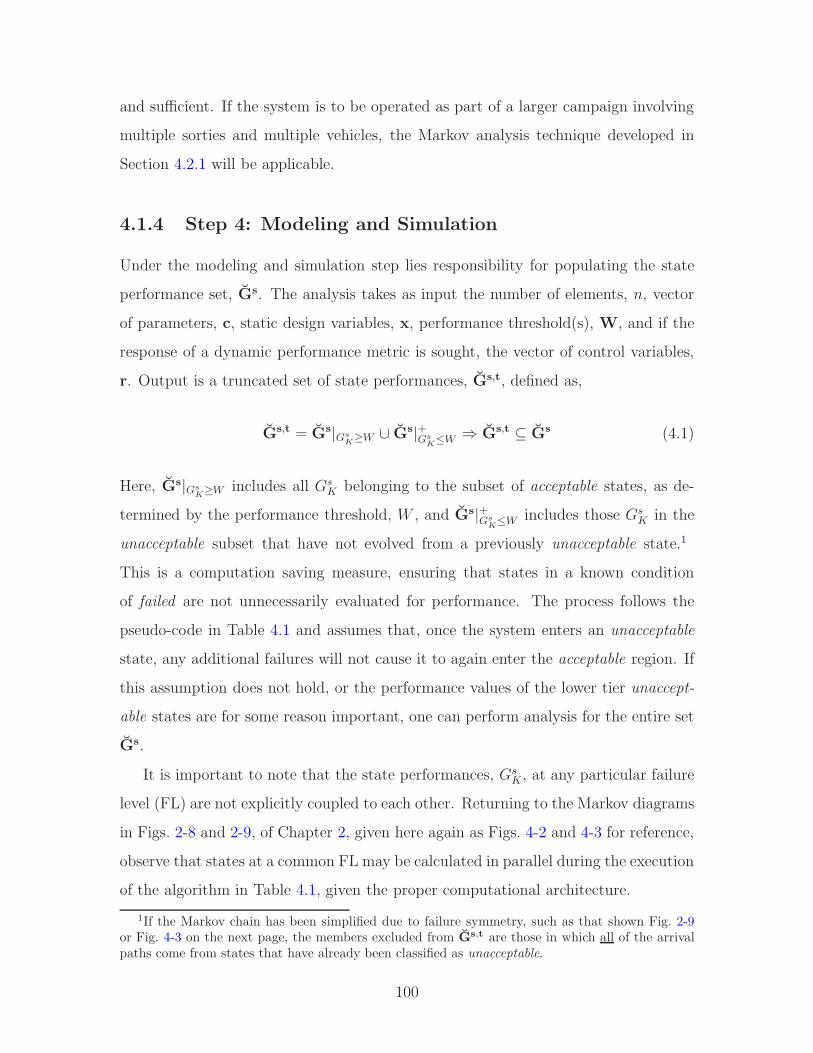
and sufficient. If the system is to be operated as part of a larger campaign involving
multiple sorties and multiple vehicles, the Markov analysis technique developed in
Section 4.2.1 will be applicable.
4.1.4 Step 4: Modeling and Simulation
Under the modeling and simulation step lies responsibility for populating the state
performance set, Gs. The analysis takes as input the number of elements, n, vector
of parameters, c, static design variables, x, performance threshold(s), W, and if the
response of a dynamic performance metric is sought, the vector of control variables,
r. Output is a truncated set of state performances, Gs,t, defined as,
Gs,t = Gs|GsK≥W ∪ Gs|+Gs
K≤W ⇒ Gs,t ⊆ Gs (4.1)
Here, Gs|GsK≥W includes all Gs
K belonging to the subset of acceptable states, as de-
termined by the performance threshold, W , and Gs|+GsK≤W includes those Gs
K in the
unacceptable subset that have not evolved from a previously unacceptable state.1
This is a computation saving measure, ensuring that states in a known condition
of failed are not unnecessarily evaluated for performance. The process follows the
pseudo-code in Table 4.1 and assumes that, once the system enters an unacceptable
state, any additional failures will not cause it to again enter the acceptable region. If
this assumption does not hold, or the performance values of the lower tier unaccept-
able states are for some reason important, one can perform analysis for the entire set
Gs.
It is important to note that the state performances, GsK , at any particular failure
level (FL) are not explicitly coupled to each other. Returning to the Markov diagrams
in Figs. 2-8 and 2-9, of Chapter 2, given here again as Figs. 4-2 and 4-3 for reference,
observe that states at a common FL may be calculated in parallel during the execution
of the algorithm in Table 4.1, given the proper computational architecture.
1If the Markov chain has been simplified due to failure symmetry, such as that shown Fig. 2-9or Fig. 4-3 on the next page, the members excluded from G
s,t are those in which all of the arrivalpaths come from states that have already been classified as unacceptable.
100
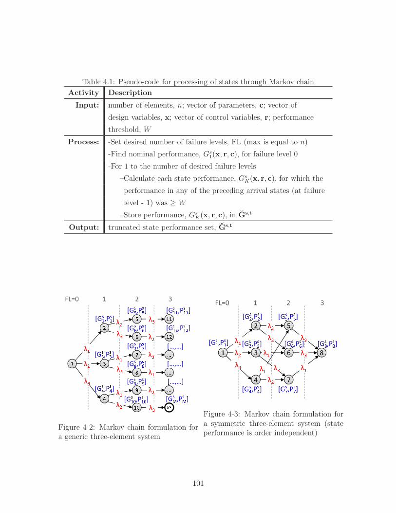
Table 4.1: Pseudo-code for processing of states through Markov chain
Activity Description
Input: number of elements, n; vector of parameters, c; vector of
design variables, x; vector of control variables, r; performance
threshold, W
Process: -Set desired number of failure levels, FL (max is equal to n)
-Find nominal performance, Gs1(x, r, c), for failure level 0
-For 1 to the number of desired failure levels
–Calculate each state performance, GsK(x, r, c), for which the
performance in any of the preceding arrival states (at failure
level - 1) was ≥ W
–Store performance, GsK(x, r, c), in Gs,t
Output: truncated state performance set, Gs,t
C D EFG
HI
λJλKλL MN
CHCCOOO[…,…]
PQλKλL λKλLλJλR λL
λJλJλK λK
λL […,…]
[GST,PST][…,…]
[GSK,PSK][GSL,PSL][GSU,PSU] CV
[GSW,PSW][GSX,PSX][GSY,PSY][GSZ,PSZ][GS[,PS[][GSJ\,PSJ\]
[GSJJ,PSJJ][GSJK,PSJK]FL=0 1 2 3
Figure 4-2: Markov chain formulation fora generic three-element system
1 3 6
5
8
7
2
4
λ]λ^λ_
λ_λ_ λ_λ]
λ] λ^λ^ λ]λ^[G],P]] [G`,P`]
[G_,P_][Ga,Pa] [Gb,Pb]
[Gc,Pc][Gd,Pd][Ge,Pe]
FL=0 1 2 3
Figure 4-3: Markov chain formulation fora symmetric three-element system (stateperformance is order independent)
101
Additionally, if massively parallel processing is available, the time saved by avoid-
ing analysis of states in a known condition of failed may be less than the increase
in time required to analyze the FL’s in series (as is done through the process in Ta-
ble 4.1). Under this circumstance, it is advantageous to concurrently calculate the
entire set, Gs, and categorize the state performances a posteriori. This will often be
the case for smaller numbers of states and if the symmetry simplification has been
made, depending on the available number of processors.
4.1.5 Step 5: Markov Analysis
Input to Step 5 are the truncated state performance set, Gs,t, and the transition
rates, λs and µs. It returns as output the set of state probabilities, Ps, calculated
through Markov analysis as described in Chapter 2, and the multistate performance
indices given in Eqns. 2.25 and 2.26. If a campaign type analysis is desired, this may
be performed according to the process described in Section 4.2.1.
4.1.6 Step 6: Analysis and Visualization of Results
Steps 4 and 5, above, may be performed on a single design point, as part of a Design-
of-Experiments (DOE) analysis, or within an optimization routine. In each case, they
have the potential to generate very large amounts of data. The number of system
evaluations will be on the order of M x d, where M is the number of system states
and d is the number of design point evaluations. Because of this, efficient analysis
of data becomes very important and results from each system and state evaluation
should be stored, when possible. Although the indices of expected performance and
availability provide an aggregated measure of performance, observing individual state
performances often helps deduce the design cause of a particular state behavior. This
provides intuition into the design problem and insight regarding updates to future
design cycles.
Visualizing results is best done through one of three means, depending on the type
of design analysis performed. Examples of each of these are given in the case studies
102
throughout the thesis. The first is a graphical representation of design sensitivities, as
already demonstrated in Chapter 3. These sensitivities are typically normalized local
gradients that reflect how the performance metric of interest changes w.r.t. changes
in each of the design variables (or component failure rates and parameters, if desired).
This visualization is best suited to the analysis of a particular point within the design
space, i.e., for the improvement of an existing design or more detailed refinement after
a general solution has been found. It provides valuable information to the designer
regarding how to best improve the design.
A second means of observation requires systematically sampling the design space
through one or more DOE methods. There are several statistical techniques avail-
able for this, including orthogonal arrays [54], Latin-hypercube spacing [62], or full-
factorial design, to name a few. Each has advantages and disadvantages, but the
general intent is to maximize coverage across design space boundaries and charac-
terize the global behavior of output with respect to input(s). Orthogonal arrays are
especially suited for determining the main effects of design variables on system out-
put, but generally require the evaluation of more design points than Latin-hypercube
spacing, for the same degree of coverage across the design space. Latin-hypercube
spacing, on the other hand, has the advantage that it provides a balance between
spreading the design points out to the maximum distance possible while maintaining
relatively uniform spacing between them.
Finally, when performing multistate design analysis as part of an optimization
routine, there are several measures of performance that should be considered in de-
termining an “optimum” solution. These include the system availability, EA, the
expected performance, EG, nominal performance, Gs1(N), and cost, if available. Com-
paring these outputs is accomplished by the pairwise plotting of their respective
Pareto fronts,2 which are composed of the design points that cannot be improved
without decrementing performance in at least one of the outputs (the non-dominated
points) [85]. There are a number of algorithms available for the optimization-based
2It is possible to compare multiple objective outputs in the form of a multidimensional Paretofront, but with higher dimensions the visual analysis is much more difficult.
103

determination of Pareto fronts, including the Adaptive Weighted Sum approach [61]
and the Normal Boundary Intersect (NBI) method [33], which is particularly suitable
for parallel computation. Special consideration must be given to the optimization of
EA, as described in Section 4.2.2.
4.2 Supporting Methods
The above section detailed the steps of multistate analysis and design, as shown in
framework of Fig. 4-1. The following two sections serve dual purposes in support of
this. They provide more detailed descriptions of subprocesses under theMarkov Anal-
ysis and Optimization blocks within the computational analysis methods of Fig. 4-1.
They also address the two specific focus areas highlighted at the end of Chapter 3.
Correspondingly, the sample problem described in Section 4.2.1 below provides an in-
depth example of the Markov analysis process in general, in addition to demonstrating
the multilayer extension to campaign analysis.
4.2.1 Multilayer Extension of Markov Analysis
The multilayer campaign analysis method proposed here is intended as a means of
translating vehicle level metrics into measures of multistate campaign performance.
This demonstrates how the multistate design of shorter duration vehicles can directly
affect longer term operational measures such as mission availability, attrition, and
sortie aborts. The technique is is possible through Markov chain formulations when
the campaign level metric of interest has direct roots in the performance output of
the vehicle level system. This is often the case, as in unmanned surveillance missions
requiring omnipresence over the mission area, or reconnaissance scan missions that
must cover a certain distance per time period. First, a short description of related
methods is provided, followed by an overview of the process, as shown in Fig. 4-4,
and a detailed detailed numerical example.
There are few references to such hierarchical modeling of discrete-state continuous-
time Markov chains in literature. One area is that of cyclic dynamics in the field of
104

physics, where reference is made to multilayer Markov chains for use in modeling
polymers in shear flow [44]. Here, the layers span across different dimensions of space
(x-direction and y-direction), rather than time, and states are not aggregated, as in
the herein described procedure. Another area is that dealing with redundancy mod-
eling in reliability analysis, where what is referred to as a hierarchical Markov model
is used to combine the techniques of redundancy modeling, at the lower level, with
the upper level system-based Markov models [59]. Application of both of the above
mentioned methods to the problem of extending vehicle level performance metrics to
a extended time campaign analysis is limited, at best.
fg hijklmi nopqrsnrtim uhnnv wg xrpyki z{|ksomi}ynopqrs nrtimuxznnv~g �o��ok�}z{|ksomi}y nopqrsnrtim u�znnv���pi�oyilr��r} misim�okm|pi poyi����pi�oyi o}t �olq��rmsi yr �iy i{|ks�omi}y �okm|pi poyi� ������ ������ ������������������� �������� �������������
�������� ��������������������� � �� ���������� ������� ������������Figure 4-4: Multi-layer Markov analysis procedure
Returning to Fig. 4-4, the first step in the procedure is to create a vehicle level
Markov model (VMM) fully representing the functional behavior of the vehicle system
in the campaign appropriate failure states. Given component failure rates, λV MM ,
the state probabilities, PVMM, are then determined using the methods described in
Section 2.3.2 of Chapter 2.3
Once the vehicle state probabilities and performances are determined, the next
step is to form the Sortie Equivalent Markov Model (SEMM). This is accomplished
by aggregating the vehicle state probabilities into probability bins, the divisions of
which are determined by performance criteria on the vehicle or mission’s objective of
interest. For instance, typical performance categories at the sortie level are nominal
(N), degraded (D), abort (A), and loss (L). The correct binning of probabilities into
3In this first step, PVMM and λV MM correspond to the sets PS and λS , defined in previous
sections.
105
the SEMM results in PSEMM, making it possible to back-solve the Markov chain for
equivalent transition rates, λSEMM , between the binned sortie states.
The above is accomplished by forming the SEMM such that each state is entered
through a unique chain of transitions. This ensures there are no more thanKSEMM−1
unknown equivalent transition rates, where KSEMM is the number of SEMM states.
It follows that a unique solution for λSEMM exists, taken from the system of ODEs
describing the SEMM Markov chain. This solution is most easily determined through
the least squares minimization problem in Eqn. 4.2,
minλSEMM
MSEMM∑
K=1
‖P (λSEMM)K − P SEMMK ‖2 (4.2)
where P(λSEMM ) is the solution to Eqn. 2.23 in Chapter 2.
The final step involves relating the sortie level transition rates, λSEMM , to the
transition rates for the Campaign Equivalent Markov Model (CEMM), which include
both λCEMM and µCEMM . In most cases, the members of λCEMM may be de-
termined by summing members of λSEMM that occur at common levels of failure
and enter states of the same performance category. Otherwise, the unknown CEMM
rates can be organized such that they are solvable through Eqn. 4.2 as before. The
set µCEMM represents campaign equivalent repair rates by way of sortie regener-
ation and replacement. These repair rates are known values derived from average
sortie duration, logistics of the particular mission scenario, and available campaign
infrastructure. Finally, the probabilities, PCEMM, are found through the solution of
Eqn. 2.23 for the CEMM.
The following step-by-step procedure is prescribed for the above:
1. Given λV MM , solve vehicle level Markov system to obtain GVMM, PVMM.
a) Aggregate members of PVMM into probability bins based on sortie level
performance categories defined by W = [Wmin,N Wmin,D Wmin,A]. This
provides PSEMM.
b) Check thatMSEMM∑
K=1
P SEMMK = 1.
106

2. Form Sortie Equivalent Markov Model (SEMM) with the unknown set, λSEMM ,
and PSEMM from above.
a) Check that each state, K, results from a unique chain of transitions.
b) Solve SEMM by operating on Eqn. 2.23 with the least squares minimization
in Eqn. 4.2 to obtain values for λSEMM .
3. Form Campaign Equivalent Markov Model (CEMM) with λCEMM , µCEMM ,
and the unknown set, PCEMM, the divisions of which are based on campaign
level performance categories defined by W = [Wmin,N Wmin,D].
a) Determine λCEMM by summing members of λSEMM that occur at common
levels of failure and enter states of the same SEMM performance category.
b) Determine µCEMM from campaign level logistics.
c) Solve CEMM through Eqn. 2.23 to obtain PCEMM.
The following example demonstrates the above process on a simple four component
air vehicle reconnaissance system, and provides a more in-depth view of the Markov
solution process. The system has an endurance of 40 hours and takes part in a 5-year
multiple sortie campaign to map a land mass located 10 hours away from its home
base. Its components, A, B, C, D, compose λV MM and have failure rates of:
• λA = 1/500hrs
• λB = 1/500hrs
• λC = 1/200hrs
• λD = 1/300hrs
The vehicle’s operational velocity is 240 nm/hr and the failure of each respective
component decrements the velocity according to the schedule given in Table 4.2.
Table 4.3 provides the values for cases where certain order and set dependent failures
decrement the velocity. For instance, if the state is defined by only two failures,
arrived at by the failure of Element A followed by failure of Element D (A→D), the
107
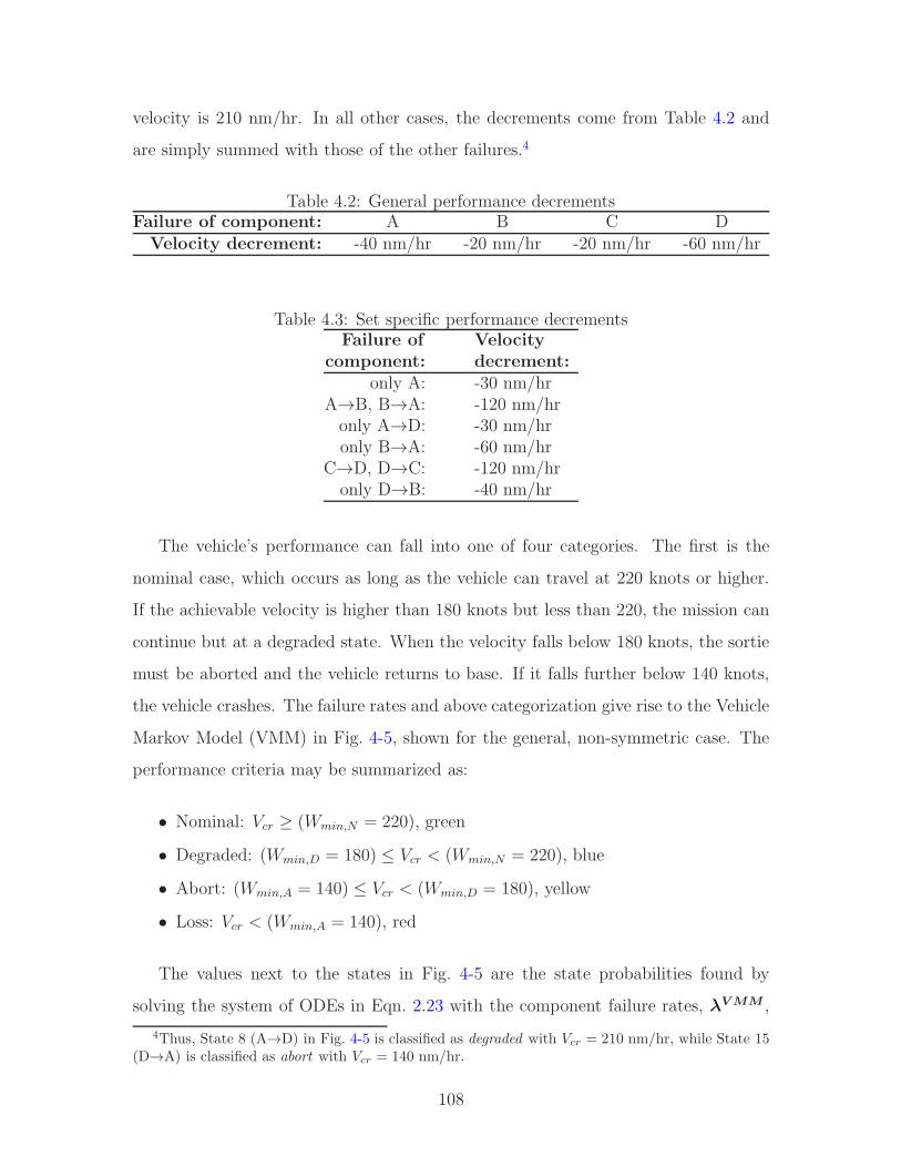
velocity is 210 nm/hr. In all other cases, the decrements come from Table 4.2 and
are simply summed with those of the other failures.4
Table 4.2: General performance decrementsFailure of component: A B C DVelocity decrement: -40 nm/hr -20 nm/hr -20 nm/hr -60 nm/hr
Table 4.3: Set specific performance decrementsFailure of Velocity
component: decrement:only A: -30 nm/hr
A→B, B→A: -120 nm/hronly A→D: -30 nm/hronly B→A: -60 nm/hr
C→D, D→C: -120 nm/hronly D→B: -40 nm/hr
The vehicle’s performance can fall into one of four categories. The first is the
nominal case, which occurs as long as the vehicle can travel at 220 knots or higher.
If the achievable velocity is higher than 180 knots but less than 220, the mission can
continue but at a degraded state. When the velocity falls below 180 knots, the sortie
must be aborted and the vehicle returns to base. If it falls further below 140 knots,
the vehicle crashes. The failure rates and above categorization give rise to the Vehicle
Markov Model (VMM) in Fig. 4-5, shown for the general, non-symmetric case. The
performance criteria may be summarized as:
• Nominal: Vcr ≥ (Wmin,N = 220), green
• Degraded: (Wmin,D = 180) ≤ Vcr < (Wmin,N = 220), blue
• Abort: (Wmin,A = 140) ≤ Vcr < (Wmin,D = 180), yellow
• Loss: Vcr < (Wmin,A = 140), red
The values next to the states in Fig. 4-5 are the state probabilities found by
solving the system of ODEs in Eqn. 2.23 with the component failure rates, λV MM ,
4Thus, State 8 (A→D) in Fig. 4-5 is classified as degraded with Vcr = 210 nm/hr, while State 15(D→A) is classified as abort with Vcr = 140 nm/hr.
108

¡¢ £ ¤¥¦ §¨§¤£§£©ª §§§© £ª£££«£¬¬ §¬§£§ª £¦£¥£¨£¤« §¦§«§¥ ª§ª©ªªª£
§ ¡¡®¡¯
¡
¡¡
¡ ¡¡¡
¡¢¡¢¡¢
¡¢ ¡¢¡¢¡¢
¡®¡®¡®
¡®¡®¡®
¡¯¡¯
¡¯¡¯¡®¡¯¡¯¡¯
Vehicle component failure rates:
- λ° = failure rate of component A, 1/500hrs- λ± = failure rate of component B, 1/500hrs- λ² = failure rate of component C, 1/200hrs- λ³ = failure rate of component D, 1/300hrs
´µ¶·´µ ¸·´µ ¸·
´µ·¹¸´µ º»
´µ ´¶´µ ´¼´µ ´½ µ ´¼µ ´¶´µ ´½µ ´¶µ ·´µ ´¶´µ ´½´µ ·´µ ´½
´µ ´´¼´µ ´´¹´µ ´´·´µ ´´¹´µ ´´¹´µ ´´¹´µ ´´¼´µ ´´·´µ ´´¼´µ ´´¹´µ ´´¼´µ ´´¹´µ ´´·´µ ´´·´µ ´´¹´µ ´´¹
Figure 4-5: Vehicle Markov Model (VMM)
and the vehicle’s design endurance time as inputs. They represent the probability
that the system will find itself in that particular state at the end of the operational
period defined by the vehicle’s endurance. Having solved the VMM for both the
performance, GVMM, and probabilities, PVMM, it is now possible to form the sortie
equivalent model by aggregating the VMM probabilities such that one may solve
for SEMM equivalent transition rates, λSEMM , through Eqn. 4.2. The criteria on
vehicle performance were established above as applied to the sortie model, therefore
the remaining task is to organize the transition paths such that the rates may be
uniquely defined by the SEMM state probabilities. The nominal and degraded states
are fairly straightforward in this example, given by,
P SEMMN = P VMM
1 + P VMM3 + P VMM
4 (4.3)
P SEMMD = P VMM
2 + P VMM5 + P VMM
8 + P VMM10 + P VMM
14 + P VMM17 (4.4)
where P SEMMN and P SEMM
D refer to the nominal and degraded states in Fig. 4-6.
109

¾¿ÀÁÀ
 ¿ÃÁÃÁÄ ÁÅ
λÆÇλÆÈ λÆÉ
λÆÇÉλÆÇÈλÆÉÈ λÆÇÉÈ Sortie equivalent states:
- N = Nominal- D = Degraded- A = Sortie Abort- L = Loss of Vehicle
ÊËÌÍÌÊËÎÏÐÊËÊÊÍÊËÊÎÑ
ÊËÊÊÍÊËÊÎÒ ÊËÊÊÊÓÊËÊÊÊÓFigure 4-6: Sortie Equivalent Markov Model (SEMM)
The abort and loss states are a little more complicated due to the various paths
possible, but may be determined in a similar manner. For example, state K = A2 in
the SEMM (Fig. 4-6) is the abort state defined by the receiving path N → D →, and
its probability calculated as,
P SEMMA2
= P VMM7 + P VMM
15 (4.5)
State L3 is the loss state defined by the receiving path N → A → (found as
green→yellow→ in the VMM), and calculated as,
P SEMML3
= P VMM24 + P VMM
25 + P VMM26 + P VMM
27 (4.6)
The complete SEMM is shown in Fig. 4-6, with the summed probabilities shown next
to the states.5 Sorting and summing of the probabilities, such as that done in the
above four equations, is very complex when done algorithmically for an unknown
number of states with varying performance distributions. The algorithm developed
for this has been included in Appendix C.
Given the state probabilities in the SEMM, the equivalent transition rates are
5Displayed probabilities may be slightly off due to rounding.
110

found by solving Eqn. 4.2, where P SEMMK are the values from Fig. 4-6. This results
in the equivalent transition rates given in Table 4.4
Table 4.4: SEMM equivalent transition ratesValue
λSEMM [1/hr]λND 1/194.2λNA 1/3454λNL 1/2763λNDL 1/237.3λNDA 1/335.0λNAL 1/239.8λNDAL 1/158.4
The SEMM equivalent transition rates may now be used to determine λCEMM
through the summations next to the campaign model in Fig. 4-7. To understand these,
note that the campaign itself is now viewed as the system, with its own performance
output that depends on the operational status of its constituent elements. In this
example, the real-time campaign performance metric of interest is the rate at which
mapping data is collected over the land mass in nautical miles per hour. Since only
a single vehicle is required to operate over the land mass at a time, this rate is the
velocity of the operating vehicle, which might be in a nominal or degraded state.
From the campaign standpoint, when the vehicle aborts or crashes, no data is being
collected and therefore the campaign is in a failed state until another aircraft arrives.
ÔÕÖ××ØÕÖ××ÙÕÖ××
λÚÛλÛÜ
λÚÜμÛÚ
μÜÚFrom SEMM:
- {λÚÛ}ÝÞßß = {λÚÛ}àÞßß = 1/194.2hrs- {λÛÜ}ÝÞßß = {λÚÛá}àÞßß + {λÚÛâ}àÞßß = 1/138.9hrs - {λÚÜ}ÝÞßß = {λÚá}àÞßß + {λÚâ}àÞßß = 1/1535hrs- {μÛÚ }ÝÞßß= f(average sortie duration) = 1/20hrs- {μÜÚ }ÝÞßß= f(reaction time + sortie
ingress duration) = 1/(72hrs + 10hrs)
ãäåæçãäãèãäéå
Figure 4-7: Campaign Equivalent Markov Model (CEMM)
111

The repair rates, µCEMM , are functions of sortie duration, travel time to and
from the land mass, and the reaction time required for the operators of the system to
respond. A safe estimate of the repair rate from the degraded to the nominal state
in this example, µDN , is the inverse of 1/2 the average sortie duration, since it is
assumed that any failure is just as likely to occur at the beginning of the mission as
near the end,6 and the vehicle continues operation unless it has reached the abort
state. If the vehicle aborts or crashes, one can assume that the operators would take
some time to determine the cause of the abort or crash before sending a replacement
vehicle, so as not to repeat it. Therefore, the repair rate, µFN , is merely the inverse
of this reaction time plus the sortie ingress duration.
With the transition rates determined, the members of PCEMM are found in the
traditional manner through Eqn. 2.23, for the campaign time of 5-years. These are
given as the numbers next to the states in Fig. 4-7. The expected performance in each
of the CEMM states can be derived from the VMM in order to obtain performance
outputs for the overall campaign. The expected nominal performance, GCEMMN , is
calculated through Eqn. 4.7,
GCEMMN =
∑
GV MMK
≥220
GVMMK
P VMMK
∑
GV MMK
≥220
P VMMK
(4.7)
summing only the nominal states in the VMM. A similar procedure is used to find
GCEMMD and GCEMM
F , remembering to account for the fact that both abort and loss
states fall into the failed category in the CEMM, and that if the campaign performance
metric of interest requires the vehicle to be operating over the land mass, the failed
performance is by definition zero. The results from this example are: GCEMMN =235
NM/hr, GCEMMD =206 NM/hr, and GCEMM
F =0 NM/hr. Eqn. 4.8 is used to determine
6This assumption stems from those made in defining a Markov process, namely that the transitionrate distribution is not time dependent. In the case where this does not apply, it is still possibleto solve for the state probabilities through what is known as a semi-Markov process [69], whereEqn. 2.23 is composed of linear integral equations rather than ODEs.
112

the total campaign expected performance, ECEMMG ,
ECEMMG =
MCEMM∑
K=1
GCEMMK PCEMM
K = 151nm/hr (4.8)
and campaign expected availability is ECEMMA = PCEMM
N + PCEMMD = 65%. The
above solutions allow derivation of several additional measures of performance, the
mechanics of which may depend on specific campaign logistics. The total expected
science distance covered over the 5-year campaign is 6.4 million mapping miles. This
is determined by multiplying the expected campaign mapping rate by the 5-year time
period, and accounting for science mile loss due to additional ingress/egress required
for sortie aborts and losses. These are the only times in which there is not a vehicle
over the continent. The probabilities of an abort or loss state from the SEMM is
1.8% and 2.9%, respectively, which can be used to estimate the total number of
vehicles lost over the campaign. In this case, with an average sortie duration at
a little less than 40 hours, of which half is spent over the land mass, 1378 sorties
will be used to cover the 6.4 million miles. One can expect 25 sortie aborts and
40 vehicles to be lost. When integrated with an accurate vehicle model, the above
methodology accurately represents campaign performance output and attrition as a
function of component failure rates, vehicle static design variables, endurance, speed,
and campaign architecture.
4.2.2 Optimization of System Availability
The final topic of this chapter moves from the Point Design/DOE block of com-
putational analysis in Fig. 4-1 to that of Optimization. While the main focus of the
research is design analysis, rather than optimization, in some cases a numerically opti-
mal solution for system availability may be desired. This is necessary for determining
a Pareto front through one of the optimization-based methods given in Section 4.1.6,
or if the designer is solely interested in the absolute maximum attainable value of EA.
A formal optimization statement for maximizing EA (for Tz = T ) is given in
113

Eqn. 4.9.
given parameters, c
transition rates,λs
minimize − EA(x, c) =∑
GsK(x,c)≥W
−P sK(λ
s)
s.t. h(x, c) = 0
g(x, c) ≤ 0
xi,LB ≤ xi ≤ xi,UB i = 1, 2, ..., nx
(4.9)
where the inequality in the summation indicates that only those state probabilities
corresponding to states with performance greater than or equal to W are summed.
This results in EA being a piecewise constant function. To show this visually, the
Gaussian function in Eqn. 4.10 was constructed and modified to model the perfor-
mance of a multistate system with six failure modes (see Appendix D for more details
on how this was accomplished).
GsK(x) =(1− 0.4u1K(x))
2e−(0.4u1K(x))2−(u2
K(x)+1)2
...− 10(4u1K(x)− 0.5u2K(x)4)e−(0.4u1
K(x))2−u2
K(x)2
...− e−(4u1K(x)−2)2−u2
K(x) − 0.3(0.8u1K(x) + u2K(x))
(4.10)
where x = [x1 x2]. Figure 4-8 graphically shows the output space of this function for
expected availability characterized by GsK ≥ 3.0, evaluated for all sixty-four states.
Gradient-based optimization algorithms will have extreme difficulty forming search
paths through the performance space in Fig. 4-8 and will exhibit very poor conver-
gence, if they converge at all. There are heuristic methods capable of searching such
non-smooth functions, but they are generally less efficient than the gradient methods,
and do not provide the same valuable sensitivity information to the designer.
Fortunately, there are certain characteristics of the availability function that en-
able one to adapt the problem for a gradient-based solution. First, improvement
of availability directly requires increasing performance in the off-nominal states to a
114
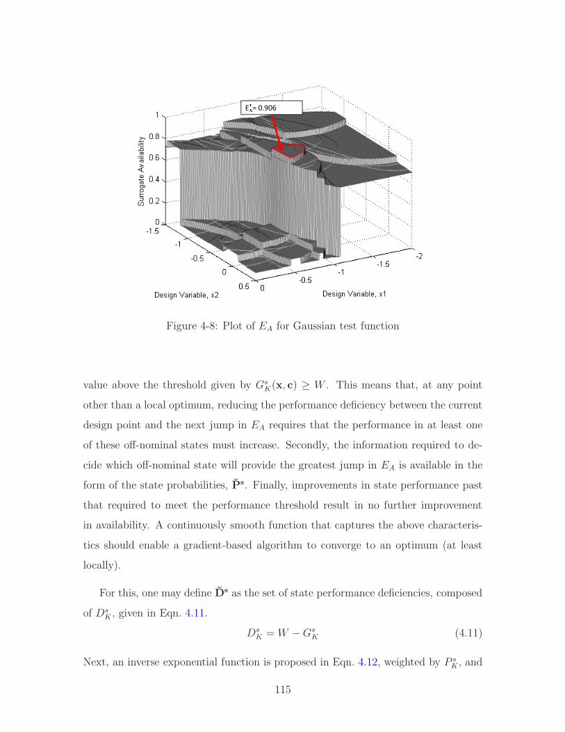
Eêë= 0.906
Figure 4-8: Plot of EA for Gaussian test function
value above the threshold given by GsK(x, c) ≥ W . This means that, at any point
other than a local optimum, reducing the performance deficiency between the current
design point and the next jump in EA requires that the performance in at least one
of these off-nominal states must increase. Secondly, the information required to de-
cide which off-nominal state will provide the greatest jump in EA is available in the
form of the state probabilities, Ps. Finally, improvements in state performance past
that required to meet the performance threshold result in no further improvement
in availability. A continuously smooth function that captures the above characteris-
tics should enable a gradient-based algorithm to converge to an optimum (at least
locally).
For this, one may define Ds as the set of state performance deficiencies, composed
of DsK , given in Eqn. 4.11.
DsK = W −Gs
K (4.11)
Next, an inverse exponential function is proposed in Eqn. 4.12, weighted by P sK , and
115

modified such that improvements in GsK beyond W are non-influential.
SEA=
M∑
K=1
P sKB where B =
b
b(max[1+DsK,1])
(4.12)
The term B has the effect of modeling transitions between levels of availability, and
the exponent base, b, determines the degree of smoothing between those transitions.
Figure 4-9 shows B for several different exponent bases.
0 0.5 1 1.5 2 2.5 3 3.5 4 4.5 50
0.1
0.2
0.3
0.4
0.5
0.6
0.7
0.8
0.9
1
Performance Deficiency, D
B
b = 2
b = e
b = 10
b = 100
Figure 4-9: Plot of B for several different exponent bases, b
Equation 4.12 may be thought of as a surrogate representation of EA.7 It is a
function of the same variables and maintains the same three characteristics described
7Although arrived at through different processes, Eqn. 4.12 is in some ways similar to theKreisselmeier-Steinhauser (KS) function, which uses a logarithmic (base e) summation to aggre-gate constraints into a single objective for gradient-based optimization [63]. Both use a type of‘shaping’ or ‘draw-down’ factor (such as b), with the distinct difference that Eqn. 4.12 approachesthe exact surface of EA as b goes to infinity, while the KS function approaches only the value of amaximum constraint as its ‘draw-down’ factor approaches infinity. Thus, the surrogate EA accu-rately models each of the individual aggregated elements, while the KS function only models one(the max constraint) at any given point in the design space. Logarithmic functions for the surrogateEA were also tested but a solution could not be found that was both bounded by the interval [0,1]and distributive such that P s
K could be used as a multiplier.
116

above. It smooths the availability function, depending on b, and may be used within
a gradient-based optimization routine. The degree of smoothness is left up to the
designer, but general good practice is to run one optimization across the entire design
space with a relatively low value of b. This corresponds to gently sloping transitions
between EA levels and should result in a solution near the region of highest EA. This
is due to the fact that the surrogate EA function effectively models the general shape
of the actual EA even when its approximated value at any give point is not highly
accurate (note the comparison of surfaces between Figs. 4-10 and 4-11). Once this
solution is found, b may be increased and a second optimization run for more accurate
results.
Figures 4-10 and 4-11 show plots of SEAfor the Gaussian problem, with two
different values of b. Even though the plots are smoothed and might not fully match
the real EA function values, the region of optimal design in Fig. 4-8 encompasses the
optimal design points above, and their optimal values are within 0.3%. Additionally,
the Gaussian functions in this example are extremely non-linear (purposefully), and
many functions would require much less smoothing.
Figure 4-12 shows a plot of the Pareto front for SEAvs. EG, with the exact solution
for EA shown on the rightmost y-axis. The front was successfully calculated using
the Normal Boundary Intersect (NBI) method, with b = 100.
117

xì= [-0.70, -0.37]Sìíî = 0.908
Figure 4-10: Output space of surrogate availability function, SEA, b = 100
xï= [-0.75,-0.37]Sïðñ = 0.907
Figure 4-11: Output space of surrogate availability function, SEA, b = 1000
118
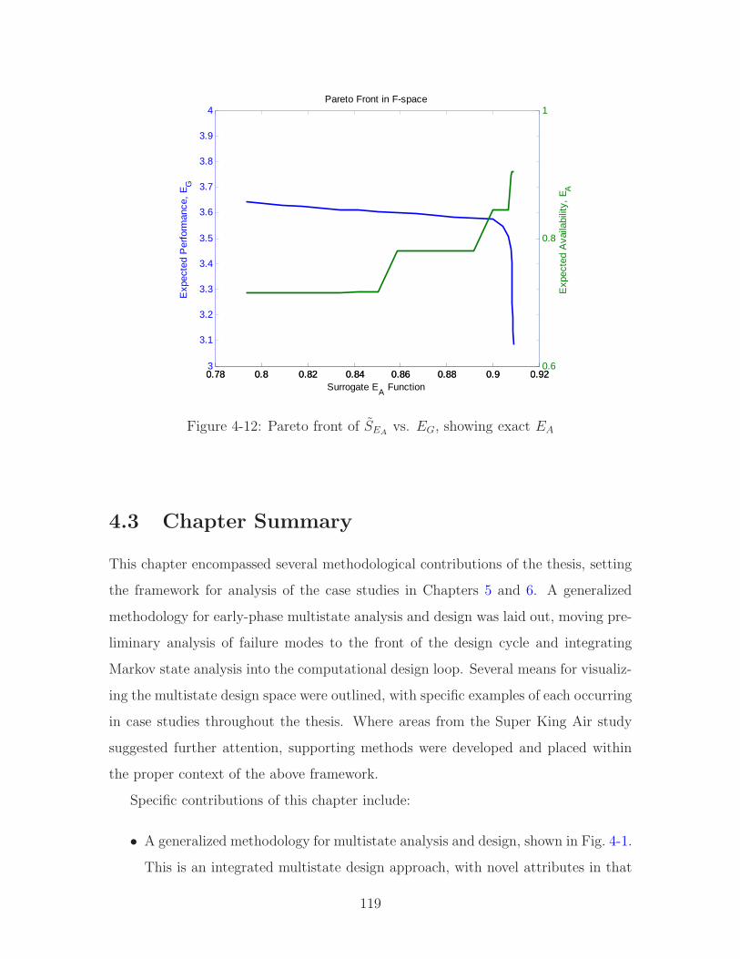
0.78 0.8 0.82 0.84 0.86 0.88 0.9 0.923
3.1
3.2
3.3
3.4
3.5
3.6
3.7
3.8
3.9
4Pareto Front in F-space
Exp
ecte
d P
erfo
rman
ce,
EG
Surrogate EA
Function0.78 0.8 0.82 0.84 0.86 0.88 0.9 0.92
0.6
0.8
1
Exp
ecte
d A
vaila
bilit
y, E
A
Figure 4-12: Pareto front of SEAvs. EG, showing exact EA
4.3 Chapter Summary
This chapter encompassed several methodological contributions of the thesis, setting
the framework for analysis of the case studies in Chapters 5 and 6. A generalized
methodology for early-phase multistate analysis and design was laid out, moving pre-
liminary analysis of failure modes to the front of the design cycle and integrating
Markov state analysis into the computational design loop. Several means for visualiz-
ing the multistate design space were outlined, with specific examples of each occurring
in case studies throughout the thesis. Where areas from the Super King Air study
suggested further attention, supporting methods were developed and placed within
the proper context of the above framework.
Specific contributions of this chapter include:
• A generalized methodology for multistate analysis and design, shown in Fig. 4-1.
This is an integrated multistate design approach, with novel attributes in that
119
it:
– formulates responses in system expected performance and availability as
functions of static design variables and component failure rates, accounting
for control design variables where appropriate
– integrates Markov state analysis into the early-phase computational design
loop for complex systems, and
– moves preliminary analysis of failure modes and effects to the front of the
design cycle.
• A multilayer extension of Markov analysis, for translating single sortie compo-
nent and vehicle level availability to multiple sortie mission campaign robust-
ness. This demonstrates how the multistate design of shorter duration vehicles
can directly affect longer term operational measures such as mission availability,
attrition, and sortie aborts.
• The development and demonstration of a “surrogate” function for system avail-
ability. The function is adjustable for differing degrees of smoothness and allows
the otherwise discrete metric to be optimized via gradient-based optimization
algorithms (Fig 4-12).
120
Chapter 5
Case Study - II: Long Endurance
Unmanned Aerial Vehicle
This chapter applies the methodologies formalized in Chapter 4 to the design and
analysis of a long endurance unmanned aerial vehicle. Case requirements come from
a representative UAV ice surveillance mission over Antarctica, under consideration at
NASA as a complement to the current IceBridge campaign, an operation currently
executed through a series of missions flown by a Douglas DC-8 and a Lockheed P-3
Orion. The analysis is performed for two scenarios. Scenario I is the case of a mission
lasting three months time aloft, which demonstrates the effectiveness of the approach
to an ultra long duration vehicle. In this scenario, an initial design point is chosen
from a study of long endurance UAV technologies recently performed at NASA. This
aircraft is optimized for nominal performance and compared to design spaces for
the same aircraft designed for multistate performance through: a) variation of only
its up-front static static design variables, b) variation of only its component failure
rates, and c) combined multistate approach varying both. Scenario II is the case of a
one-to-two day duration vehicle, involved in a 5-year multi-sortie campaign requiring
omnipresence over the continent. This demonstrates application of the approach to
shorter duration systems involved in ultra long duration campaigns where coverage
is provided by multiple vehicles. In this scenario, the design space is systematically
sampled via a Design of Experiments technique, allowing examination of the main
121

effects of design variables on campaign level performance metrics.
Results clearly showed three distinct design spaces for the ultra long endurance
aircraft designed through a), b), and c) above. The combined multistate approach
demonstrated improvement in system availability of 11%, at a 3% lower cost, when
compared to the baseline aircraft designed for nominal performance. Variation of
component failure rates or static design variables alone showed improvement of only
6.5%. Furthermore, when considering multiple objectives of system availability, ex-
pected performance, nominal performance, and cost, the combined approach was still
able to achieve an 11% improvement in availability, with only a 4.5% decrease in
nominal performance, albeit at a small 6% increase in aircraft flyaway cost. Finally,
results from the multi-sortie campaign analysis demonstrated that lower level static
design variables have a clear and measurable effect on campaign level performance,
such as availability, number of failed sorties, and vehicles lost. The effects of these
variables do not necessarily align with the effects they have on nominal performance.
The next several sections follow the steps laid out in the multistate analysis and
design process shown in Fig. 4-1, of Chapter 4.
5.1 Step 1 - Requirements Definition and Concept
of Operations
Requirements for this case study are derived from a representative UAV mission to col-
lect mapping data over the ice sheets of Antarctica. This mission began several years
ago with the launch of NASA’s Ice, Cloud, and Land Elevation Satellite (ICESat)
in 2003. Data collected by the satellite are providing a long duration time-history
of ice sheet mass balance, as well as important information concerning clouds and
aerosol height in the observation area. In 2009, ICESat stopped collecting data when
the last of three lasers on the satellite’s Geoscience Laser Altimeter System (GLAS)
ceased emitting light [80]. After several attempts to restart the lasers, the satellite
was decommissioned in August of 2010. The launch of a replacement system is not
122

planned until 2015.
NASA is currently attempting to cover this 6-year gap through a series of flights
using a Douglas DC-8 and a Lockheed P-3 Orion [79]. While this solution is capable
of minimally covering the transitional period until 2015, data coverage is sporadic and
requires the use of expensive resources and aircrews. This has motivated NASA into
considering other methods, such as long endurance UAVs, to provide much better data
coverage for future gaps and perhaps eventually replace satellite operations altogether.
The analysis in this chapter begins from results of a preliminary study at NASA,
which suggests that a favorable base of operations for a long-endurance UAV campaign
to Antarctica is from the Falkland Islands off the southern tip of South America [103].
The original intent of the campaign was to match the data point density of that
obtained by ICESat. However, an alternative ground track based on a grid pattern
was found to be sufficient in that it met the continental edge point density of the
satellite while being much more efficient from the standpoint of an aircraft. Based on
this ground track and the required edge point density, approximately 100,000 total
nautical miles (nm) over-continent are required to complete one survey of the land
mass. The average distance to the area of operations from the chosen base location
is 2100 nm. A simplified diagram of the survey area, including the base of operations
is shown in Fig. 5-1.
~2100 nm
tot. coverage ~ 100000 nm
Falklands
Figure 5-1: Antarctica survey area and pattern
123
Operational requirements for the air vehicle are partially driven by the environ-
mental conditions necessary for mapping the ice sheets and partially by the vehicle’s
concept of operations. Wind data averages over Antarctica indicate that minimum
winds aloft velocity occurs between altitudes of 45k to 55k ft, and a much smaller
altitude band at 60k ft (± 500 ft). Although the 60k ft band is more desirable from
an efficiency standpoint, the wind speed rises rapidly outside of this 1000 ft band.
Even with the uncertainties involved in nominal operations, such small tolerances
are undesirable, and exceedingly more so when considering operation in off-nominal
states. Therefore, the target altitude in nominal operations is set at 50k ft.
In the first concept of operations, referred to throughout the remainder of the
chapter as Scenario I, the ice surveillance mission is performed by a single ultra long
endurance vehicle over the three months of Antarctic summer. This represents a
mission carried out with what NASA considers the nearest-horizon technology for
ultra long endurance aircraft, namely a liquid-hydrogen proton exchange membrane
(LH2-PEM) fuel cell, here augmented with solar-regeneration to extend endurance
during the sun-intense summer. More on this may be found in an extensive study
published by NASA in [83].
The second concept of operations (Scenario II ) represents a multiple sortie cam-
paign to continuously map the ice sheets over a time period of 5-years. The aircraft
involved have endurance on the order of 40+ hours, which is at the high end of
current in-production UAVs utilizing internal combustion engines [2]. This scenario
maintains omnipresence over the continent, such that as Aircraft 1, shown in Fig. 5-2,
comes to the end of its surveillance period, Aircraft 2 arrives over the operations area.
On average, the ingress/egress distance is about 2100 nm, allowing fully functional
air vehicles to remain over continent for approximately 20 hrs.
Table 5.1 presents a summary of the requirements for both Scenarios I and II.
Some of the performance minimums are relaxed for the Scenario I aircraft, due to
the more demanding endurance requirement. However, there still exist certain hard
limits that stem from the environment. For example, the 95 kt minimum airspeed is
to allow the aircraft enough maneuvering airspeed to overcome expected winds aloft
124
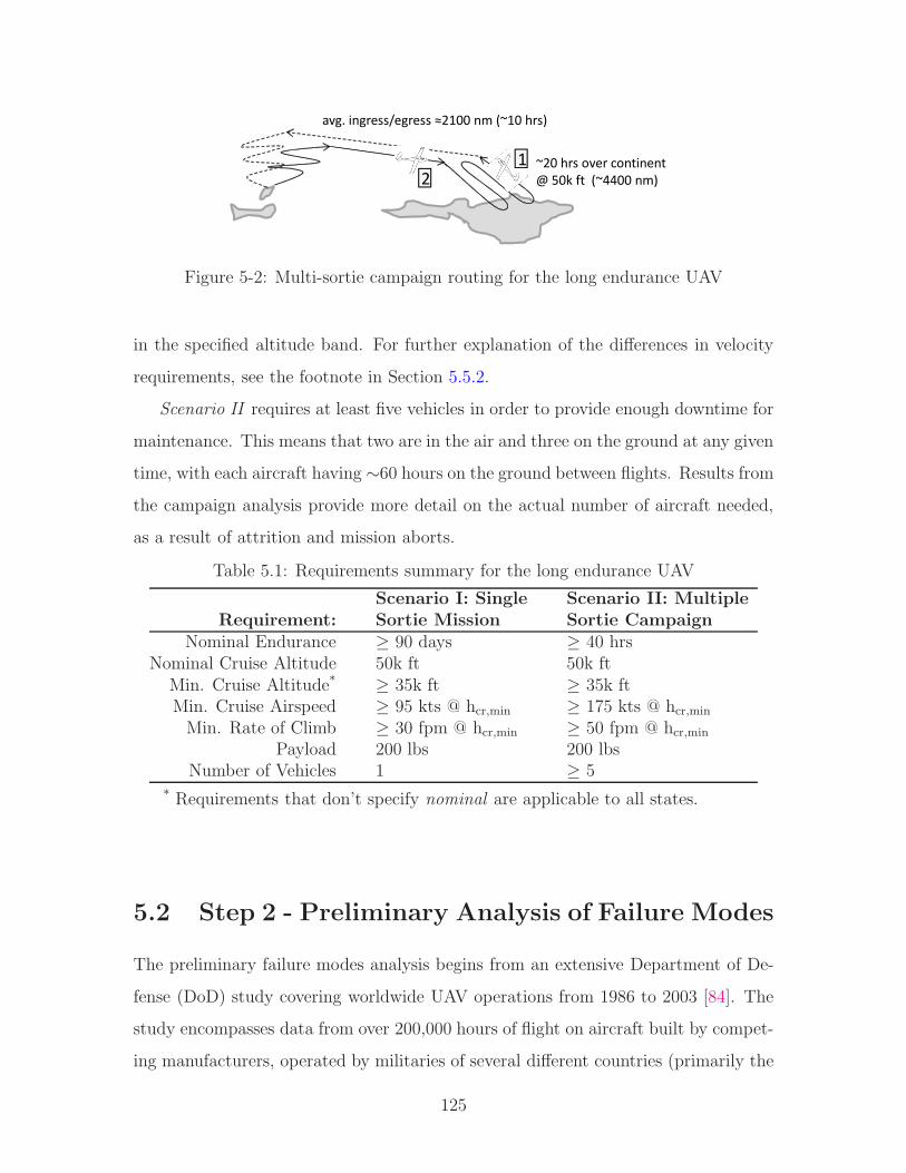
~20 hrs over continent@ 50k ft (~4400 nm)
avg. ingress/egress ≈2100 nm (~10 hrs)
21
Figure 5-2: Multi-sortie campaign routing for the long endurance UAV
in the specified altitude band. For further explanation of the differences in velocity
requirements, see the footnote in Section 5.5.2.
Scenario II requires at least five vehicles in order to provide enough downtime for
maintenance. This means that two are in the air and three on the ground at any given
time, with each aircraft having ∼60 hours on the ground between flights. Results from
the campaign analysis provide more detail on the actual number of aircraft needed,
as a result of attrition and mission aborts.
Table 5.1: Requirements summary for the long endurance UAV
Scenario I: Single Scenario II: MultipleRequirement: Sortie Mission Sortie Campaign
Nominal Endurance ≥ 90 days ≥ 40 hrsNominal Cruise Altitude 50k ft 50k ft
Min. Cruise Altitude* ≥ 35k ft ≥ 35k ftMin. Cruise Airspeed ≥ 95 kts @ hcr,min ≥ 175 kts @ hcr,min
Min. Rate of Climb ≥ 30 fpm @ hcr,min ≥ 50 fpm @ hcr,min
Payload 200 lbs 200 lbsNumber of Vehicles 1 ≥ 5
* Requirements that don’t specify nominal are applicable to all states.
5.2 Step 2 - Preliminary Analysis of Failure Modes
The preliminary failure modes analysis begins from an extensive Department of De-
fense (DoD) study covering worldwide UAV operations from 1986 to 2003 [84]. The
study encompasses data from over 200,000 hours of flight on aircraft built by compet-
ing manufacturers, operated by militaries of several different countries (primarily the
125
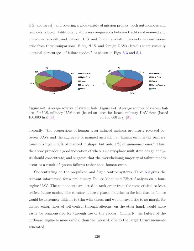
U.S. and Israel), and covering a wide variety of mission profiles, both autonomous and
remotely piloted. Additionally, it makes comparisons between traditional manned and
unmanned aircraft, and between U.S. and foreign aircraft. Two notable conclusions
arise from these comparisons. First, “U.S. and foreign UAVs (Israeli) share virtually
identical percentages of failure modes,” as shown in Figs. 5-3 and 5-4.
òóôõöô÷óô ÷÷ô øô ùúûüýþùýúÿ������ �ú��ýú��ú�����þ�ýú� ����
Figure 5-3: Average sources of system fail-ures for U.S. military UAV fleet (based on100,000 hrs) [84]
��������� ��� �� ������������ !"# $�%#���$�&&'(&)%�*��(%+, -.
Figure 5-4: Average sources of system fail-ures for Israeli military UAV fleet (basedon 100,000 hrs) [84]
Secondly, “the proportions of human error-induced mishaps are nearly reversed be-
tween UAVs and the aggregate of manned aircraft, i.e., human error is the primary
cause of roughly 85% of manned mishaps, but only 17% of unmanned ones.” Thus,
the above provides a good indication of where an early-phase multistate design analy-
sis should concentrate, and suggests that the overwhelming majority of failure modes
occur as a result of system failures rather than human error.
Concentrating on the propulsion and flight control systems, Table 5.2 gives the
relevant information for a preliminary Failure Mode and Effect Analysis on a four-
engine UAV. The components are listed in rank order from the most critical to least
critical failure modes. The elevator failure is placed first due to the fact that its failure
would be extremely difficult to trim with thrust and would leave little to no margin for
maneuvering. Loss of roll control through ailerons, on the other hand, would more
easily be compensated for through use of the rudder. Similarly, the failure of the
outboard engine is more critical than the inboard, due to the larger thrust moments
generated.
126
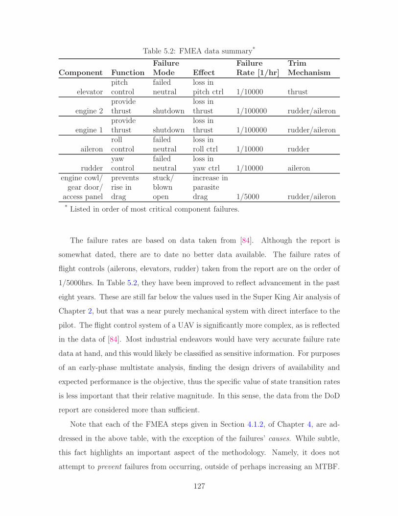
Table 5.2: FMEA data summary*
Failure Failure TrimComponent Function Mode Effect Rate [1/hr] Mechanism
pitch failed loss inelevator control neutral pitch ctrl 1/10000 thrust
provide loss inengine 2 thrust shutdown thrust 1/100000 rudder/aileron
provide loss inengine 1 thrust shutdown thrust 1/100000 rudder/aileron
roll failed loss inaileron control neutral roll ctrl 1/10000 rudder
yaw failed loss inrudder control neutral yaw ctrl 1/10000 aileron
engine cowl/ prevents stuck/ increase ingear door/ rise in blown parasite
access panel drag open drag 1/5000 rudder/aileron* Listed in order of most critical component failures.
The failure rates are based on data taken from [84]. Although the report is
somewhat dated, there are to date no better data available. The failure rates of
flight controls (ailerons, elevators, rudder) taken from the report are on the order of
1/5000hrs. In Table 5.2, they have been improved to reflect advancement in the past
eight years. These are still far below the values used in the Super King Air analysis of
Chapter 2, but that was a near purely mechanical system with direct interface to the
pilot. The flight control system of a UAV is significantly more complex, as is reflected
in the data of [84]. Most industrial endeavors would have very accurate failure rate
data at hand, and this would likely be classified as sensitive information. For purposes
of an early-phase multistate analysis, finding the design drivers of availability and
expected performance is the objective, thus the specific value of state transition rates
is less important that their relative magnitude. In this sense, the data from the DoD
report are considered more than sufficient.
Note that each of the FMEA steps given in Section 4.1.2, of Chapter 4, are ad-
dressed in the above table, with the exception of the failures’ causes. While subtle,
this fact highlights an important aspect of the methodology. Namely, it does not
attempt to prevent failures from occurring, outside of perhaps increasing an MTBF.
127
Therefore, the determination of the failure’s cause is not the focus, but rather the
mitigation of its effect, given that it occurs and does so at a predictable rate.
5.3 Step 3 - System and Performance Classifica-
tion
Step 3 of the methodology requires classifying the system according to its level of
analysis, and determining whether the performance metric is dynamic or static. In
this particular case study, results will be given for both levels of analysis, the UAV
system modeled at the single vehicle level (Scenario I ), and at the multiple sortie
campaign level (Scenario II ). This demonstrates the differences between the two, and
shows how the procedures from the lower level may be integrated into those of the
higher.
The performance metric of interest is, naturally, endurance. While possible to
run an entire flight mission using the same simulation routines and methods as in the
case study of Chapter 3, the endurance is less affected by dynamic influences over the
long flight duration and is readily modeled through the static, physics-based analytic
equations in the next section. For this reason, the control variables, r, are not used in
the following analyses. The analytic equations assume the system is controllable, as
is often done in conceptual level design. This process allows a more rapid evaluation
of system states and thus facilitates the timely analysis of larger design spaces.
5.4 Step 4 - Modeling and Simulation
This step is divided into two subsections. The first subsection describes the analyt-
ical methods used in calculating elements of the multistate performance set, Gs, for
the long endurance UAV. The second presents the cost model used in determining
aircraft flyaway cost, a useful metric in comparing the relative expense of changes in
component failure rates to changes in static design variables. Step 4 is the same for
both Scenario I and Scenario II.
128

5.4.1 Multistate Performance Model
The aircraft model disciplines follow closely those of the Super King Air in Chapter 2.
The exception is that the UAV multistate performance model computes endurance
through iterated analysis of analytic equations, rather than simulation. This follows
the general design flow depicted in Fig. 5-5, and is described in greater detail below.
Geometry
Mass Properties
Engine
Aero
Throttle
Controls/TrimControls/
TrimControls/TrimControls/
TrimControls/TrimControl/
TrimK
Range/Endur-ance
/0123456789:;89<=>9?@9A8B<=C
8<DB=BDBE98:BD>:;F
GH540H5 IJ 0146K55LM02H1H3L5 /I4 N56H 5JL340JO5IKHP 02HMQ52IO1HRPerformance
S T Q5OHI4 I/ IK540H1IJ02 K040U5H546V T Q5OHI4 I/ 6H0H1O L561WJ Q0410N256XY T Q5OHI4 I/ H40J61H1IJ 40H56Z 61[5 \] ^ _ ` ` a IKHP L40WKI204 b
,
c c dG G� �
Figure 5-5: Design flow for ultra long endurance UAV
Endurance is calculated from Eqn. 5.1, which is the Breguet range equation [25]
divided by the aircraft’s cruise velocity.
GsK = EnduranceK =
ηpropVcr,Kc
(CL
CD
)Kln(W1
W2) (5.1)
Here, ηprop is the propeller efficiency, c is power specific energy consumption, and
W1
W2is the ratio of the aircraft’s weight at the beginning of the cruise segment over
its weight at the end. The Vcr,K and ( CL
CD)K terms are the aircraft’s state specific
cruise velocity and lift-to-drag ratio, respectively. Given the desired Mach number
at cruise, the performance analysis iterates on altitude until induced drag is equal to
129

three times the parasite drag, or,
C2L,K
πeA = 3CDo,K (5.2)
This is the level-flight condition for minimum power required in a propeller driven
aircraft. In the case of an aircraft consuming combustible fuel, the analysis also ac-
counts for decreasing weight, resulting in a cruise-climb to maintain the conditions
of Eqn. 5.2.1 Additionally, the analysis accounts for the case of a state with insuffi-
cient power at altitude, by reducing altitude and allowing Mach number to vary until
min-power conditions are maintainable. The iterative processes are shown in Fig. 5-6.efghi j kl mlnopoqr sopoqr tquvwxqyz{|}{z~� t ��� �����}������ ���}���� z~ syz{|}{z~� �� � �p ����v���xvr �uo�xv�pr ��� � � � �p � � �
t � tquvwxq � ����� ���v � ��v � highi j s�v�o¡x¢£r��v¢£r ¤£r ¥¦§¨�©¦ª�£
�v « �v ¬ �v�u « �u ¬ �us « s ¬ s
®¯®¯ °±² ° ±²
®¯n � n³op �®¯° ±²°±²
s « sopoqtquvw « tquvw ´ tquvwr n « n ´ n
µ¶·¸
� « §�©¹s « ©º»¼»¨§�t « t©ªsn « ��¼¹s»� « �s��»»º�� « §�½ º�ª»¼�¦�� « ��ºº¼¦¹ ¾�¾�¦»�p « ��ºº¼¦¹ ¾�¾�¦»
� « � ¬ �Figure 5-6: Iterative processes in UAV performance model
1In level, unaccelerated flight, the lift coefficient, CL, varies directly with aircraft weight. There-fore, to maintain the optimum cruise velocity for minimum power required, an aircraft must climbas it burns off fuel.
130

The trim algorithms developed for the innermost loop (1) of Fig. 5-6 are fairly
sophisticated and were derived from work under a 1998 NASA grant to calculate
engine-out stability derivatives [51]. These methods were extended to include ad-
ditional control surface failures, in support of this research, using analytic stability
derivative equations developed from the 6-DOF equations of motion, as found in [90].
They are prerequisite to the outer loop processes (2,3,4) of Fig. 5-6 in that each state,
K, must be trimmed for steady, level flight at each altitude and airspeed iteration.
This is accomplished through the trim routine that takes as input the aircraft de-
sign vector, failure mode, and flight conditions, and returns the state specific control
deflections required to drive the roll and yaw moments to zero. It also returns the
corresponding state specific drag polar for that particular altitude and airspeed iter-
ation, which is then used to calculate the state specific endurance, range, and other
important performance outputs.2 Appendix E provides more detail on the above
methods, including sample output of the state performances.
5.4.2 Cost Model
The cost model is developed from three separate sources. The first of these is the
RAND Corporation’s Development and Procurement Cost of Aircraft model (DAPCA
IV), as found in [86]. The DAPCA IV model uses cost estimating relationships
based on historical data and aircraft physical properties to estimate various costs
including engineering, tooling, manufacturing, and quality control, among others. In
general, the DAPCA related cost data presented in Section 5.6 follows the functional
dependency given in Eqn. 5.3:
Cost ↑ ≈ f(S ↑,A ↑,Λ ↑, λ ↑, Pmax ↑, Nengines ↑,Wempty ↑) (5.3)
Several updates have been made to the above model over the years, including those to
more accurately predict costs for unmanned aerial vehicles, using more recent UAV
2Although these iterative processes are quite involved, evaluation of 64 states for a single designpoint takes only about 30 seconds on a high-end computer, and is very robust. All of the designpoints attempted in this study converged without problem.
131

cost data found in [57] and [109]. Some results using these updates are published
in [2].
The DAPCA IV model estimates cost for the basic air vehicle. The second two
sources for the overall cost model involve estimating the dollar cost of changes to
component failure rates. The Charles Stark Draper Laboratory, a sponsor of this
research, recently led a study to relate similar subsystem components of differing
complexity and MTBF to their respective costs [112]. While the focus of the study
was on space systems, the MTBF vs. cost data involved a more general sampling of
avionics and control hardware for aerospace systems. Without specifying the exact
proprietary costs or mean-times-between-failure, the study findings are shown in the
trend plots of Fig. 5-7.
¿ÀÁÂÃÄÅÆÇ
¿ ¿ÈÄ À ÀÈÄ Á ÁÈÄ Â ÂÈÄ Ã ÃÈÄ Ä
Norm
alize
d Cos
t
Normalized Mean Time Between Failure
ÉÊËÌÍ ÎÏÐÑ ÒÓ Àÿ¿ ÔÊËÑÕÖ×ÍØÐÙÚ ÎÏÐÑ ÒÓÆÄ¿ ÔÊËÑÕÖÛÚÊÜÜ ÎÏÐÑ ÒÓ À¿¿ ÔÊËÑÕÖÝÍÜÐÊÞÐÜÐÑß àáÕÑ âÙÏãÑÐáÏä å æ ¿ÈÀÝÍÜÐÊÞÐÜÐÑß àáÕÑ âÙÏãÑÐáÏä å æ ¿ÈÁÝÍÜÐÊÞÐÜÐÑß àáÕÑ âÙÏãÑÐáÏä å æ ¿ÈÂ
Figure 5-7: Comparison of reliability costs for various components, normalized byaveraged cost and MTBF of Medium Unit
Figure 5-7 also depicts independent estimates from the third source [75] as the re-
liability cost functions next to the Draper data. This cost function estimates changes
in component cost as a direct function of reliability, rather then MTBF, and is given
132

as Eqn. 5.4.
C(R) = Be(1−f)R−RminRmax−R (5.4)
Here, C(R) is the cost function, f is a cost index of improving the component’s
reliability relative to other system components, Rmin and Rmax are the minimum and
maximum reliabilities feasible for the current component state-of-the-art, and B is
the baseline component cost. These f -adjusted functions are plotted alongside the
Draper data of Fig. 5-7, with reliability, R, replaced by MTBF. They demonstrate
the applicability of the cost function in estimating the current sample-derived data.
The bow-shaped nature of the cost curves stems from the fact that, beyond a certain
point, technological limits mean that improving a component’s reliability (or MTBF)
becomes asymptotically more expensive. As both data sets show, this trend increases
with increasing component complexity.
Due to the agreement between the above trends and cost estimates, Eqn. 5.4 is
used in estimating the cost variations of components with respect to MTBF in the
analyses of Section 5.6. The baseline cost value is chosen as the initial subsystem cost
output from the DAPCA IV model, with component MTBF’s as shown in Table 5.2.
This is then adjusted by Eqn. 5.4, according to the design-driven increase or decrease
in MTBF. The engines are modeled as high complexity (large unit) components, the
flight controls as moderate complexity (medium unit) components, and the access
panel/cowling as a low complexity (small unit) component.
5.5 Step 5 - Markov Analysis
The previous step established the multistate modeling and simulation routines neces-
sary for calculating the UAV’s state performance set, Gs, along with an estimate of
the corresponding cost for achieving that performance set. The members of Gs are
GsK(x, c). Step 5 now uses Markov analysis to calculate the probabilities, P s
K(λs) be-
longing the UAV’s state probability set, Ps. In the case of the campaign in Scenario
II, the probabilities are also dependent on the campaign “repair” rates, µCEMM .
Both scenarios are described in more detail below.
133

5.5.1 Scenario I: Single Sortie Mission
To this point, the Markov analysis technique for a single vehicle has been well devel-
oped in Section 2.3.2, of Chapter 2, and demonstrated in Section 3.2, of Chapter 3.
The mechanics of the process remain the same here, but with a much larger number
of states. Given a total of n = 6 elements, the size of Gs and Ps is M = 2n = 64.
Figure 5-8 is the Markov chain for States 1 through 22, truncated to the first two
levels of failure for efficiency of space. çè é ê ë ì í
î ï ð ð ð ð ð ð ð ð ð ð ð ð ð
λñòóôλõö÷øöõùúλõö÷øöõùûλüýþþõüλÿøôõüòöλõôõ�ÿ�òü
Figure 5-8: Markov chain for UAV (first two levels of failure)
The values of λs = [λcowl, λengine,1, λengine,2, λrudder, λaileron, λelevator] are those in
Table 5.2, and the model is evaluated over a time, T , equal to the aircraft’s design
endurance (∼three months). The states falling into the acceptable performance cate-
gory are those with minimum cruise velocity greater than or equal to 95 knots, which
is high enough above the maximum expected winds aloft to deliver sufficient ground
speed in the target altitude band.
5.5.2 Scenario II: Multiple Sortie Campaign
The second scenario begins with the Markov model in Fig. 5-8, but for the UAV
designed under the requirement of a 40-hour nominal flight duration. This model
is termed the Vehicle Markov Model (VMM) in the multilayer analysis, and leads
134

development of the Sortie Equivalent Markov Model (SEMM) and the Campaign
Equivalent Markov Model (CEMM) further downstream. The analysis procedure
follows that of the example described in Section 4.2.1, but with many more states
and design points.
As mentioned in Chapter 4, multiple sortie campaign analysis is possible when
the campaign level metric of interest has direct roots in the performance output of
the vehicle system. In the case of Scenario II, the campaign performance objective
is the Science Mile Accumulation Rate (SMAR), which is determined by the cruise
velocity of the individual air vehicles. From the campaign perspective, there are four
categories of performance into which the vehicle output may fall, instead of just two.
These are defined for Scenario II as:
• Nominal: Vcr ≥ (Wmin,N = 215)
• Degraded: (Wmin,D = 175) ≤ Vcr < (Wmin,N = 215)
• Abort: (Wmin,A = 90) ≤ Vmin & Vcr < (Wmin,D = 175)
• Loss: Vmin < (Wmin,A = 90)
The division point between acceptable and unacceptable states in Scenario I was
determined by the cruise speed required to continue performing the mission at alti-
tude. This corresponds to the division between the degraded and abort categories in
Scenario II.3 Nominal performance occurs when the aircraft is (near) fully functional
and may include states in which a failure does not significantly affect performance.
This corresponds to the highest rate of mapping coverage. Degraded includes states
with less than nominal airspeed but higher than the stall speed at the bottom of the
required altitude band. Finally, the vehicle is lost when its maximum velocity at sea
level falls below its approximate stall velocity of 90 knots.
The fact that the VMM state performances, GVMMK , change with each variation
in the design vector, x, requires that the summing of probabilities, P SEMMK , into
their respective SEMM performance bins (reference Eqns. 4.3 - 4.6, Chapter 4) be
3The velocity magnitudes are different (175 knots in Scenario I vs. 95 knots in Scenario II ) dueto the different sized aircraft. The 40-hour aircraft has a higher cruise speed and smaller wing area.It therefore has a significantly higher stall speed at the bottom of the required altitude band thanthe three month aircraft.
135

performed for each design point. To do so robustly, for a generalized number of states
and performances, required the development of an involved sorting and summing
algorithm, the code for which is provided in Appendix C. Numerical results for the
SEMM and CEMM models are given in Section 5.6.2.
5.6 Step 6 - Analysis and Visualization of Results
The Super King Air case study in Chapter 3 demonstrated the use of sensitivity
derivatives in determining relative effects of design variables and component failure
rates on multistate performance metrics. The presentation of results in the following
subsections takes a more global look at the design space, through the DOE and Pareto
analysis techniques listed in Step 6 of Fig. 4-1. In the case of Scenario I, visualization
occurs through a multi-objective analysis of Pareto non-dominated points, filtered
from a design space generated via Latin-hypercube spacing. This demonstrates how
the designer may visually choose preferable designs from the multi-objective design
space, and further refine through gradient-based optimization of availability using the
surrogate function introduced in Section 4.2.2, Chapter 4. In the case of Scenario
II, a DOE analysis is performed by sampling the design space through an orthogonal
array. Since the objective is to demonstrate the translation of vehicle level metrics
to the campaign level, the Scenario II analysis stops short of determining an overall
superior design, but examines instead the main effects of design variables on campaign
availability and the number of sorties failed and vehicles lost.
Each of the UAV’s in Scenarios I and II was first sized for nominal requirements,
as a starting baseline for entry into the multistate analysis and design framework. In
the case of Scenario I, this aircraft was taken from a representative example in the
NASA UAV study of [83]. The Scenario II aircraft comes from a shorter duration
UAV study in [2]. In both cases, the representative aircraft was then sized for scenario-
specific nominal performance requirements using the conceptual-level aircraft design
program described in [2]. This aircraft was used as the baseline.
Table 5.3 shows the resulting baseline aircraft design vectors, along with their
136
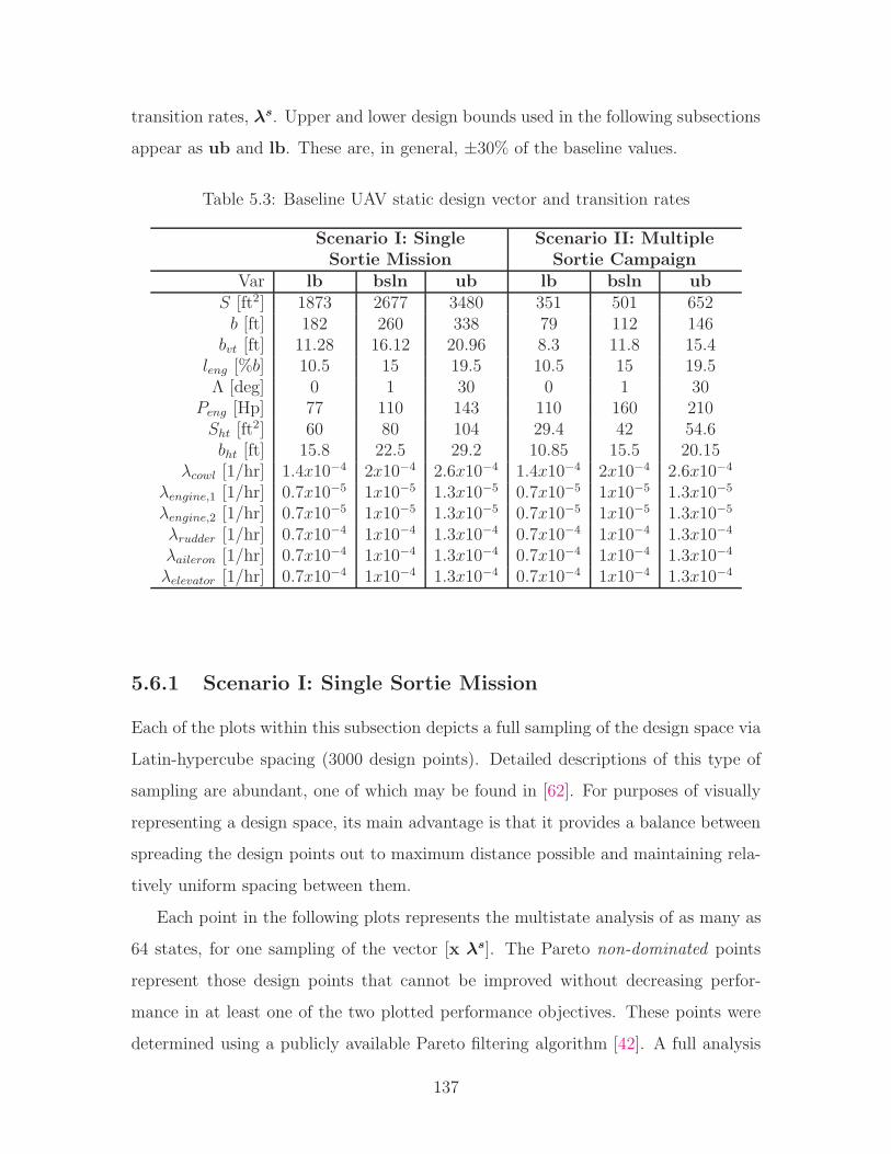
transition rates, λs. Upper and lower design bounds used in the following subsections
appear as ub and lb. These are, in general, ±30% of the baseline values.
Table 5.3: Baseline UAV static design vector and transition rates
Scenario I: Single Scenario II: MultipleSortie Mission Sortie Campaign
Var lb bsln ub lb bsln ubS [ft2] 1873 2677 3480 351 501 652b [ft] 182 260 338 79 112 146
bvt [ft] 11.28 16.12 20.96 8.3 11.8 15.4leng [%b] 10.5 15 19.5 10.5 15 19.5Λ [deg] 0 1 30 0 1 30
Peng [Hp] 77 110 143 110 160 210Sht [ft
2] 60 80 104 29.4 42 54.6bht [ft] 15.8 22.5 29.2 10.85 15.5 20.15
λcowl [1/hr] 1.4x10⁻⁴ 2x10⁻⁴ 2.6x10⁻⁴ 1.4x10⁻⁴ 2x10⁻⁴ 2.6x10⁻⁴
λengine,1 [1/hr] 0.7x10⁻⁵ 1x10⁻⁵ 1.3x10⁻⁵ 0.7x10⁻⁵ 1x10⁻⁵ 1.3x10⁻⁵
λengine,2 [1/hr] 0.7x10⁻⁵ 1x10⁻⁵ 1.3x10⁻⁵ 0.7x10⁻⁵ 1x10⁻⁵ 1.3x10⁻⁵
λrudder [1/hr] 0.7x10⁻⁴ 1x10⁻⁴ 1.3x10⁻⁴ 0.7x10⁻⁴ 1x10⁻⁴ 1.3x10⁻⁴
λaileron [1/hr] 0.7x10⁻⁴ 1x10⁻⁴ 1.3x10⁻⁴ 0.7x10⁻⁴ 1x10⁻⁴ 1.3x10⁻⁴
λelevator [1/hr] 0.7x10⁻⁴ 1x10⁻⁴ 1.3x10⁻⁴ 0.7x10⁻⁴ 1x10⁻⁴ 1.3x10⁻⁴
5.6.1 Scenario I: Single Sortie Mission
Each of the plots within this subsection depicts a full sampling of the design space via
Latin-hypercube spacing (3000 design points). Detailed descriptions of this type of
sampling are abundant, one of which may be found in [62]. For purposes of visually
representing a design space, its main advantage is that it provides a balance between
spreading the design points out to maximum distance possible and maintaining rela-
tively uniform spacing between them.
Each point in the following plots represents the multistate analysis of as many as
64 states, for one sampling of the vector [x λs]. The Pareto non-dominated points
represent those design points that cannot be improved without decreasing perfor-
mance in at least one of the two plotted performance objectives. These points were
determined using a publicly available Pareto filtering algorithm [42]. A full analysis
137

of 3000 design points required approximately 12 hours, performed in parallel across
8 processing threads on an Intel Quad i7 2.8GHz CPU.
Figure 5-9 shows the design-driven performance space for nominal endurance ver-
sus the aircraft flyaway cost, which includes Non-Recurring Expense (NRE) estimates
of manufacturing, tooling, engineering, and quality control from the models described
in Section 5.4.2. This cost has been converted to current year dollars and normalized
by that of the baseline NASA aircraft to protect proprietary data.
1700 1750 1800 1850 1900 1950 2000 2050 2100 21500.8
0.9
1
1.1
1.2
1.3
1.4
1.5
Nominal State Endurance [hr]
A/C
Fly
away
Cos
t [%
of b
asel
ine
cost
]
design points
Pareto non-dominated pntsNASA baseline design
�� �������� ����Figure 5-9: Design performance space for nominal endurance vs. A/C flyaway cost
The NASA baseline design point is displayed in Fig. 5-9, and is very close to
that which a designer would likely pick as a ‘best’ balance between cost and nominal
performance (less than 2% difference in either). This ‘best’ aircraft is shown to the
right of the plot for visual reference, characterized by a high aspect ratio (A=25) and
low wing sweep (Λ=4◦), as one would expect for such a long duration, high altitude
aircraft, designed for nominal performance.
The nominal-case performance space in Fig. 5-9 provides a reference point to which
the next three plots may be compared. The first of these is a design space analysis
for availability vs. flyaway cost, as shown in Fig. 5-10, where the NASA baseline
static design remains fixed, and component failure rates are allowed to vary across
the bounds defined in Table 5.3. Note that the increasing slope of the Pareto front
138

estimation represents the combined effects of the cost trends seen in Fig. 5-7. The
aircraft geometry shown is that of the NASA baseline, with failure rates, λs=[1/4297,
1/119588, 1/119588, 1/7819, 1/7829, 1/13013]/hr. In Fig. 5-10 only, aircraft geometry
is the same for each of the 3000 design points (only failure rates are varied).
0.68 0.7 0.72 0.74 0.76 0.78 0.8 0.820.9
0.95
1
1.05
1.1
1.15
1.2
1.25
System Availability
A/C
Fly
away
Cos
t [%
of b
asel
ine
cost
]
design points
Pareto non-dominated pntsNASA baseline failure rates
� ����� �� �������Figure 5-10: Design performance space for availability vs. cost - varying only λs
Where the above figure shows results for the design space with a constant static
design vector, x, Fig. 5-11 displays results for constant baseline λs, varying only static
0.74 0.75 0.76 0.77 0.78 0.79 0.8 0.81 0.820.85
0.9
0.95
1
1.05
1.1
1.15
1.2
1.25
1.3
1.35
System Availability
A/C
Fly
away
Cos
t [%
of b
asel
ine
cost
]
design points
Pareto non-dominated pnts
NASA baseline design
�� �������� ��� ��!Figure 5-11: Design performance space for availability vs. cost - varying only x
139

design variables. There are several very meaningful observations to make from this
figure. First, the shape of the design performance space is distinctly different from
that of Fig. 5-10. More on this will be discussed near the end of the section. Second,
the baseline design lies at a point near opposite that of the non-dominated Pareto
points for system availability. This indicates a probable trade-off between contesting
values of availability and nominal design performance, an issue examined further in
later figures. Finally, the aircraft’s static design is decidedly different from that of the
best designs in the previous two analyses. Most notable are the significantly increased
wing sweep (Λ=18◦) and larger tail (bvt=19.3 ft). Both of these are characteristics
that improve the aircraft’s ability to resist failure-driven perturbations to yaw and
roll. Higher wing sweep increases the lateral stability parameter, Clβ, decreasing the
aileron deflection required to return to wings level. The larger tail increases directional
stability, Cnβ, lessening the rudder deflection required to return to zero degrees of
sideslip. Neither of these characteristics help increase a subsonic aircraft’s nominal-
state endurance, as is demonstrated by the fact that this design has an endurance
that is 11.7% below that of the baseline aircraft (see summary in Table 5.4).
Figure 5-12 shows the performance space in which both x and λs are allowed
to vary. The resulting aircraft has a lower wing sweep and tail height (Λ=12◦ and
bvt=17.7 ft), but a higher system availability. In this case, flyaway cost is about the
same as in the previous analysis, showing that improved availability has been achieved,
to some degree, by replacing extra wing sweep and tail size with more cost effective
improvements in component failure rates.
To gain further insight into the effects of component failure rates versus static
design variables, the performance spaces for each of the three previous analyses are
overlaid upon one another in Fig. 5-13. This visually demonstrates two compelling
results. First, the achievable improvement in availability via static design variables
is nearly as large as that made via component failure rates. From the perspective of
reliability analysis, this is significant due to the fact that improvements in reliability
are nearly always sought after in the space of λs rather than affecting GsK through
changes to static design variables, x. Secondly, the inclusion of both x and λs in the
140

0.68 0.7 0.72 0.74 0.76 0.78 0.8 0.82 0.84 0.86 0.880.8
0.9
1
1.1
1.2
1.3
1.4
1.5
System Availability
A/C
Fly
away
Cos
t [%
of b
asel
ine
cost
]
design points
Pareto non-dominated pntsNASA baseline design
"# $%&$&"'# ()*+,&Figure 5-12: Design performance space for availability vs. cost - full multistate, λs
and x
design analysis allows a region of system availability to be reached that is unobtainable
via the independent variation of either one.
Table 5.4 presents a numerical summary of the above analyses. Some key ob-
servations are that the baseline improved design has the best nominal performance
with an endurance of 2109 hours, while the combined multistate design has the best
system availability with EA = 0.831. As noted, however, this comes at the expense
of an 11% decrease in nominal performance.
Table 5.4: Summary of designs for best cost and expected endurance
Design\PerformanceAvailability Endurexp Endurnom A/C Cost
[n/a] % devbsln [hr] % devbsln [hr] % devbslb % devbslnNASA Baseline 0.748 0.00% 1510 0.00% 2078 0.00% 0.00%
Baseline Improved† 0.733 -2.00% 1576 4.37% 2109 1.5% 1.47%λs Variation* 0.796 6.40% 1589 5.21% 2078 0.00% 2.94%x Variation‡ 0.797 6.54% 1425 -5.63% 1835 -11.70% -3.31%
Combined Multistate♦ 0.831 11.09% 1565 3.65% 1842 -11.32% -2.94%† Figure 5-9.* Figure 5-10.‡ Figure 5-11.♦ Figure 5-12.
141
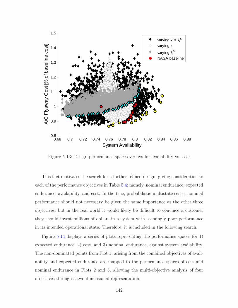
0.68 0.7 0.72 0.74 0.76 0.78 0.8 0.82 0.84 0.86 0.880.8
0.9
1
1.1
1.2
1.3
1.4
1.5
System Availability
A/C
Fly
away
Cos
t [%
of b
asel
ine
cost
]
varying x & λs
varying x
varying λs
NASA baseline
Figure 5-13: Design performance space overlays for availability vs. cost
This fact motivates the search for a further refined design, giving consideration to
each of the performance objectives in Table 5.4; namely, nominal endurance, expected
endurance, availability, and cost. In the true, probabilistic multistate sense, nominal
performance should not necessary be given the same importance as the other three
objectives, but in the real world it would likely be difficult to convince a customer
they should invest millions of dollars in a system with seemingly poor performance
in its intended operational state. Therefore, it is included in the following search.
Figure 5-14 displays a series of plots representing the performance spaces for 1)
expected endurance, 2) cost, and 3) nominal endurance, against system availability.
The non-dominated points from Plot 1, arising from the combined objectives of avail-
ability and expected endurance are mapped to the performance spaces of cost and
nominal endurance in Plots 2 and 3, allowing the multi-objective analysis of four
objectives through a two-dimensional representation.
142

0.68 0.7 0.72 0.74 0.76 0.78 0.8 0.82 0.84 0.86 0.881250
1300
1350
1400
1450
1500
1550
1600
1650
1700
System Availability
Exp
ecte
d E
ndur
ance
[hr]
Non-dominated designs for availability vs. expected endurance
Pareto non-dominated pnts
0.68 0.7 0.72 0.74 0.76 0.78 0.8 0.82 0.84 0.86 0.881700
1750
1800
1850
1900
1950
2000
2050
2100
2150
System Availability
Nom
inal
End
uran
ce [h
r]
Non-dominated designs for availability vs. nominal endurance
mapped Pareto pnts from 1
Pareto non-dominated pnts
0.68 0.7 0.72 0.74 0.76 0.78 0.8 0.82 0.84 0.86 0.880.8
0.9
1
1.1
1.2
1.3
1.4
1.5
System Availability
A/C
Fly
away
Cos
t [%
of b
asel
ine
cost
]
Non-dominated designs for availability vs. flyaway cost
mapped Pareto pnts from 1
Pareto non-dominated pnts
-. /01/1-2. 345671
89 :;<:<8=9 >?@A:<B
1
2
3
Design A
Design B
Figure 5-14: Design comparison via Pareto non-dominated points
143
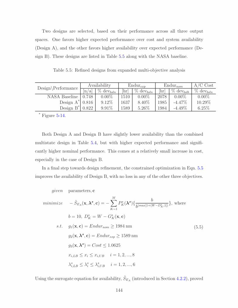
Two designs are selected, based on their performance across all three output
spaces. One favors higher expected performance over cost and system availability
(Design A), and the other favors higher availability over expected performance (De-
sign B). These designs are listed in Table 5.5 along with the NASA baseline.
Table 5.5: Refined designs from expanded multi-objective analysis
Design\PerformanceAvailability Endurexp Endurnom A/C Cost
[n/a] % devbsln [hr] % devbsln [hr] % devbslb % devbslnNASA Baseline 0.748 0.00% 1510 0.00% 2078 0.00% 0.00%
Design A* 0.816 9.12% 1637 8.40% 1985 -4.47% 10.29%Design B* 0.822 9.91% 1589 5.26% 1984 -4.49% 6.25%
* Figure 5-14.
Both Design A and Design B have slightly lower availability than the combined
multistate design in Table 5.4, but with higher expected performance and signifi-
cantly higher nominal performance. This comes at a relatively small increase in cost,
especially in the case of Design B.
In a final step towards design refinement, the constrained optimization in Eqn. 5.5
improves the availability of Design B, with no loss in any of the other three objectives.
given parameters, c
minimize − SEA(x,λs, c) = −
M∑
K=1
P sK(λ
s){ b
b(max[1+(W−DsK,1])
}, where
b = 10, DsK = W −Gs
K(x, c)
s.t. g1(x, c) = Endurnom ≥ 1984 nm
g2(x,λs, c) = Endurexp ≥ 1589 nm
g3(x,λs) = Cost ≤ 1.0625
xi,LB ≤ xi ≤ xi,UB i = 1, 2, ..., 8
λsi,LB ≤ λsi ≤ λsi,UB i = 1, 2, ..., 6
(5.5)
Using the surrogate equation for availability, SEA(introduced in Section 4.2.2), proved
144
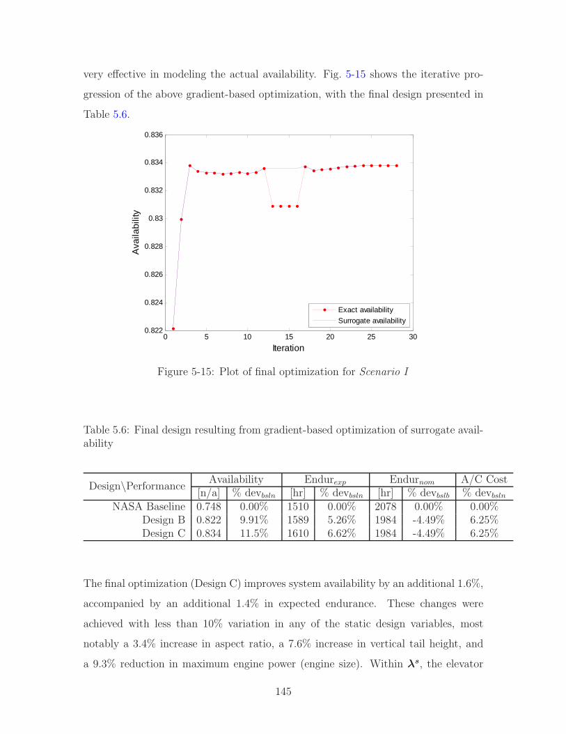
very effective in modeling the actual availability. Fig. 5-15 shows the iterative pro-
gression of the above gradient-based optimization, with the final design presented in
Table 5.6.
0 5 10 15 20 25 300.822
0.824
0.826
0.828
0.83
0.832
0.834
0.836
Iteration
Ava
ilabi
lity
Exact availability
Surrogate availability
Figure 5-15: Plot of final optimization for Scenario I
Table 5.6: Final design resulting from gradient-based optimization of surrogate avail-ability
Design\PerformanceAvailability Endurexp Endurnom A/C Cost
[n/a] % devbsln [hr] % devbsln [hr] % devbslb % devbslnNASA Baseline 0.748 0.00% 1510 0.00% 2078 0.00% 0.00%
Design B 0.822 9.91% 1589 5.26% 1984 -4.49% 6.25%Design C 0.834 11.5% 1610 6.62% 1984 -4.49% 6.25%
The final optimization (Design C) improves system availability by an additional 1.6%,
accompanied by an additional 1.4% in expected endurance. These changes were
achieved with less than 10% variation in any of the static design variables, most
notably a 3.4% increase in aspect ratio, a 7.6% increase in vertical tail height, and
a 9.3% reduction in maximum engine power (engine size). Within λs, the elevator
145
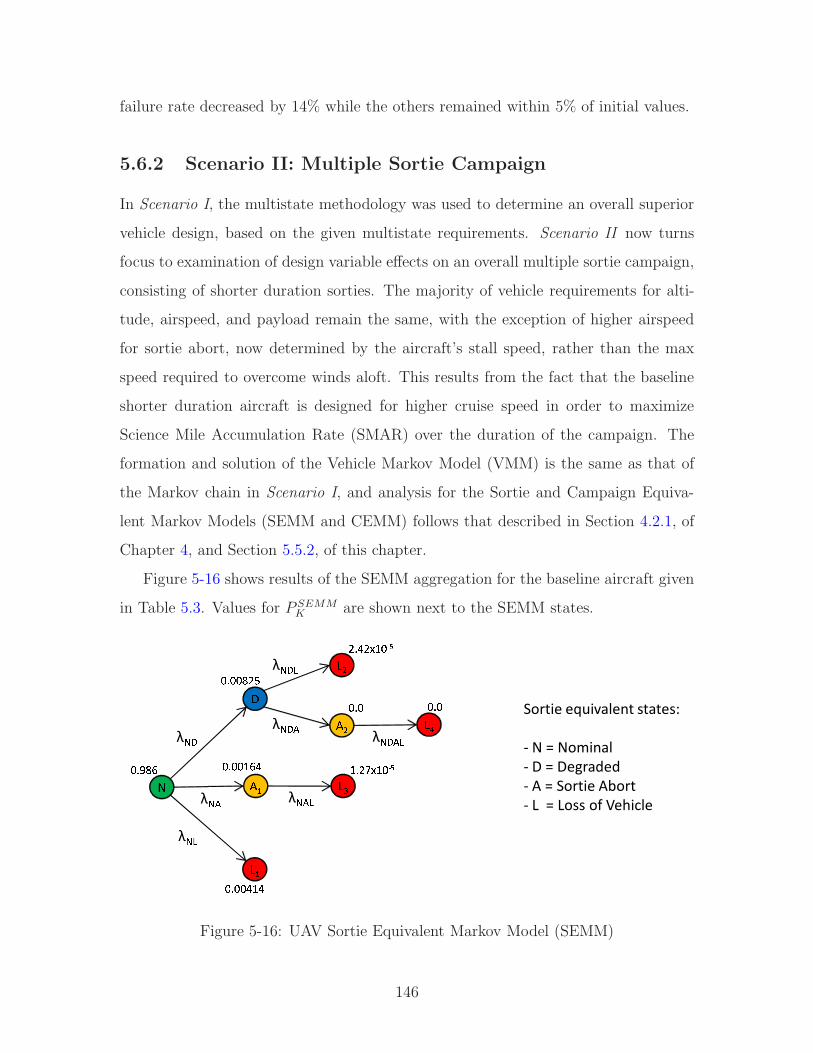
failure rate decreased by 14% while the others remained within 5% of initial values.
5.6.2 Scenario II: Multiple Sortie Campaign
In Scenario I, the multistate methodology was used to determine an overall superior
vehicle design, based on the given multistate requirements. Scenario II now turns
focus to examination of design variable effects on an overall multiple sortie campaign,
consisting of shorter duration sorties. The majority of vehicle requirements for alti-
tude, airspeed, and payload remain the same, with the exception of higher airspeed
for sortie abort, now determined by the aircraft’s stall speed, rather than the max
speed required to overcome winds aloft. This results from the fact that the baseline
shorter duration aircraft is designed for higher cruise speed in order to maximize
Science Mile Accumulation Rate (SMAR) over the duration of the campaign. The
formation and solution of the Vehicle Markov Model (VMM) is the same as that of
the Markov chain in Scenario I, and analysis for the Sortie and Campaign Equiva-
lent Markov Models (SEMM and CEMM) follows that described in Section 4.2.1, of
Chapter 4, and Section 5.5.2, of this chapter.
Figure 5-16 shows results of the SEMM aggregation for the baseline aircraft given
in Table 5.3. Values for P SEMMK are shown next to the SEMM states.
CDEFE
G DHFHFI FJ
λKLλKM λKN
λKLNλKLMλKNM λKLNM Sortie equivalent states:
- N = Nominal- D = Degraded- A = Sortie Abort- L = Loss of Vehicle
OPQRSOPOORTUOPOOVSWOPOOWVW
OPOTPWTXVOYZ OPOVPT[XVOYZFigure 5-16: UAV Sortie Equivalent Markov Model (SEMM)
146
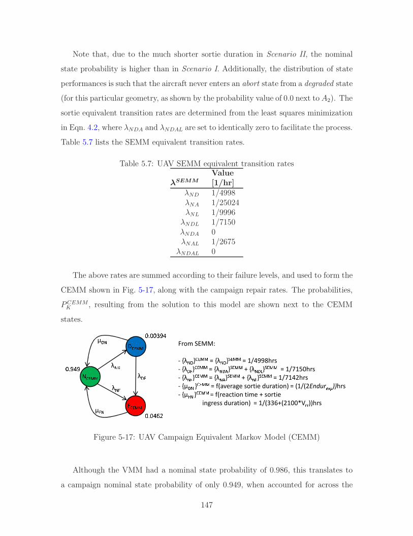
Note that, due to the much shorter sortie duration in Scenario II, the nominal
state probability is higher than in Scenario I. Additionally, the distribution of state
performances is such that the aircraft never enters an abort state from a degraded state
(for this particular geometry, as shown by the probability value of 0.0 next to A2). The
sortie equivalent transition rates are determined from the least squares minimization
in Eqn. 4.2, where λNDA and λNDAL are set to identically zero to facilitate the process.
Table 5.7 lists the SEMM equivalent transition rates.
Table 5.7: UAV SEMM equivalent transition ratesValue
λSEMM [1/hr]λND 1/4998λNA 1/25024λNL 1/9996λNDL 1/7150λNDA 0λNAL 1/2675λNDAL 0
The above rates are summed according to their failure levels, and used to form the
CEMM shown in Fig. 5-17, along with the campaign repair rates. The probabilities,
PCEMMK , resulting from the solution to this model are shown next to the CEMM
states.
\]^__ ]^__a]^__
λbcλcd
λbdμcb
μdbFrom SEMM:
- {λbc}efgg = {λbc}hfgg = 1/4998hrs- {λcd}efgg = {λbci}hfgg + {λbcj}hfgg = 1/7150hrs - {λbd}efgg = {λbi}hfgg + {λbj}hfgg = 1/7142hrs- {μcb }efgg= f(average sortie duration) = (1/(2Endurklm))hrs- {μdb}efgg= f(reaction time + sortie
ingress duration) = 1/(336+(2100*Vno))hrs
pqrsr pqpptrspqpsuv
Figure 5-17: UAV Campaign Equivalent Markov Model (CEMM)
Although the VMM had a nominal state probability of 0.986, this translates to
a campaign nominal state probability of only 0.949, when accounted for across the
147
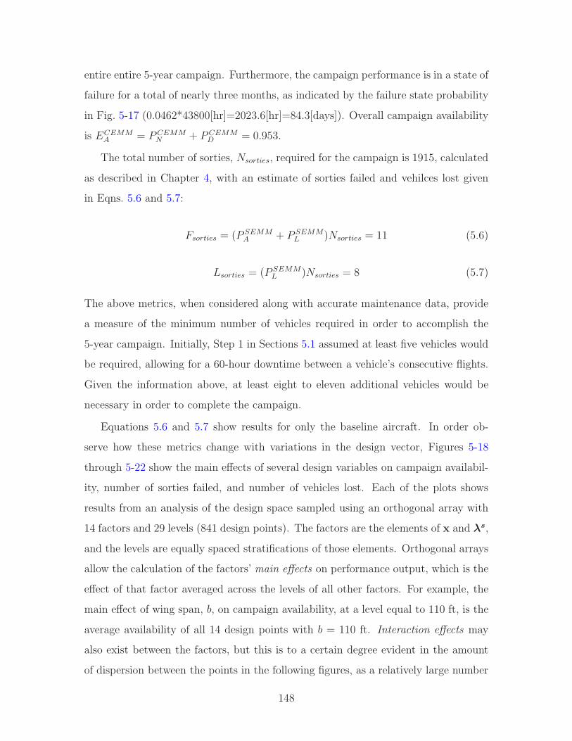
entire entire 5-year campaign. Furthermore, the campaign performance is in a state of
failure for a total of nearly three months, as indicated by the failure state probability
in Fig. 5-17 (0.0462*43800[hr]=2023.6[hr]=84.3[days]). Overall campaign availability
is ECEMMA = PCEMM
N + PCEMMD = 0.953.
The total number of sorties, Nsorties, required for the campaign is 1915, calculated
as described in Chapter 4, with an estimate of sorties failed and vehilces lost given
in Eqns. 5.6 and 5.7:
Fsorties = (P SEMMA + P SEMM
L )Nsorties = 11 (5.6)
Lsorties = (P SEMML )Nsorties = 8 (5.7)
The above metrics, when considered along with accurate maintenance data, provide
a measure of the minimum number of vehicles required in order to accomplish the
5-year campaign. Initially, Step 1 in Sections 5.1 assumed at least five vehicles would
be required, allowing for a 60-hour downtime between a vehicle’s consecutive flights.
Given the information above, at least eight to eleven additional vehicles would be
necessary in order to complete the campaign.
Equations 5.6 and 5.7 show results for only the baseline aircraft. In order ob-
serve how these metrics change with variations in the design vector, Figures 5-18
through 5-22 show the main effects of several design variables on campaign availabil-
ity, number of sorties failed, and number of vehicles lost. Each of the plots shows
results from an analysis of the design space sampled using an orthogonal array with
14 factors and 29 levels (841 design points). The factors are the elements of x and λs,
and the levels are equally spaced stratifications of those elements. Orthogonal arrays
allow the calculation of the factors’ main effects on performance output, which is the
effect of that factor averaged across the levels of all other factors. For example, the
main effect of wing span, b, on campaign availability, at a level equal to 110 ft, is the
average availability of all 14 design points with b = 110 ft. Interaction effects may
also exist between the factors, but this is to a certain degree evident in the amount
of dispersion between the points in the following figures, as a relatively large number
148

of levels was used. More on orthogonal arrays may be referenced in [54].
Figures 5-18 and 5-19 show the main effects of wingspan and maximum engine
power on campaign availability. The wingspan effect is due primarily to its influence
on aspect ratio (A = b2/S), thus there is a known interaction with wing area, S.
Regardless, one can still observe the general trend that increasing wingspan improves
availability across most of its design interval. There is a much more distinct trend
in the effect of maximum engine power, which may be thought of as the engine size.
In general, the larger engine helps increase availability up to a maximum power of
about 160 Hp, after which availability reverses trend and starts to decrease. More
detailed inspection of the performance state space shows that, in the lower region,
the larger engine prevents several state performances from falling below the mission
abort airspeed. As the engine continues to increase in size and weight, however, the
first level failure of the outboard engine results in large enough moments that the
ailerons and rudder can no longer trim for steady cruising flight at altitude. Once
this threshold crossing is broad enough that the majority of design geometries have
fallen from the degraded to abort state, the trend tapers off near the high end of the
engine power range.
80 90 100 110 120 130 140
0.76
0.78
0.8
0.82
0.84
0.86
0.88
0.9
0.92
0.94
Wingspan [ft]
Cam
paig
n A
vaila
bilit
y (m
ain
effe
ct r
espo
nse)
polynomial fit, degree-2
95% confidence bounds
Figure 5-18: Main effect of wingspan oncampaign availability
110 130 150 170 190 210 230
0.74
0.76
0.78
0.8
0.82
0.84
0.86
0.88
0.9
0.92
0.94
Max Engine Power, Pmax [Hp]
Cam
paig
n A
vaila
bilit
y (m
ain
effe
ct r
espo
nse)
polynomial fit, degree-5
95% confidence bounds
Figure 5-19: Main effect of max enginepower on campaign availability
149
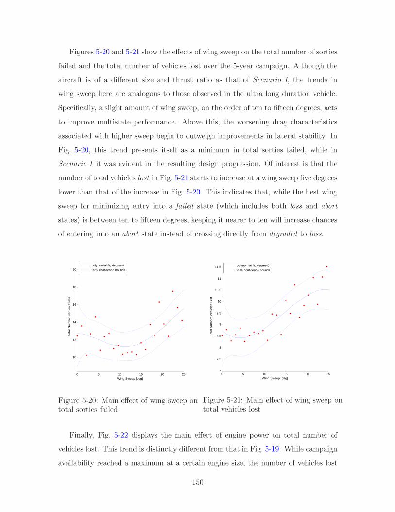
Figures 5-20 and 5-21 show the effects of wing sweep on the total number of sorties
failed and the total number of vehicles lost over the 5-year campaign. Although the
aircraft is of a different size and thrust ratio as that of Scenario I, the trends in
wing sweep here are analogous to those observed in the ultra long duration vehicle.
Specifically, a slight amount of wing sweep, on the order of ten to fifteen degrees, acts
to improve multistate performance. Above this, the worsening drag characteristics
associated with higher sweep begin to outweigh improvements in lateral stability. In
Fig. 5-20, this trend presents itself as a minimum in total sorties failed, while in
Scenario I it was evident in the resulting design progression. Of interest is that the
number of total vehicles lost in Fig. 5-21 starts to increase at a wing sweep five degrees
lower than that of the increase in Fig. 5-20. This indicates that, while the best wing
sweep for minimizing entry into a failed state (which includes both loss and abort
states) is between ten to fifteen degrees, keeping it nearer to ten will increase chances
of entering into an abort state instead of crossing directly from degraded to loss.
0 5 10 15 20 25
10
12
14
16
18
20
Wing Sweep [deg]
Tot
al N
umbe
r S
ortie
s F
aile
d
polynomial fit, degree-4
95% confidence bounds
Figure 5-20: Main effect of wing sweep ontotal sorties failed
0 5 10 15 20 257
7.5
8
8.5
9
9.5
10
10.5
11
11.5
Wing Sweep [deg]
Tot
al N
umbe
r V
ehic
les
Lost
polynomial fit, degree-5
95% confidence bounds
Figure 5-21: Main effect of wing sweep ontotal vehicles lost
Finally, Fig. 5-22 displays the main effect of engine power on total number of
vehicles lost. This trend is distinctly different from that in Fig. 5-19. While campaign
availability reached a maximum at a certain engine size, the number of vehicles lost
150
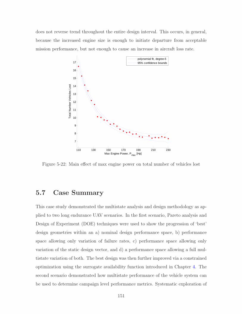
does not reverse trend throughout the entire design interval. This occurs, in general,
because the increased engine size is enough to initiate departure from acceptable
mission performance, but not enough to cause an increase in aircraft loss rate.
110 130 150 170 190 210 230
7
8
9
10
11
12
13
14
15
16
17
Max Engine Power, Pmax
[Hp]
Tot
al N
umbe
r V
ehic
les
Lost
polynomial fit, degree-5
95% confidence bounds
Figure 5-22: Main effect of max engine power on total number of vehicles lost
5.7 Case Summary
This case study demonstrated the multistate analysis and design methodology as ap-
plied to two long endurance UAV scenarios. In the first scenario, Pareto analysis and
Design of Experiment (DOE) techniques were used to show the progression of ‘best’
design geometries within an a) nominal design performance space, b) performance
space allowing only variation of failure rates, c) performance space allowing only
variation of the static design vector, and d) a performance space allowing a full mul-
tistate variation of both. The best design was then further improved via a constrained
optimization using the surrogate availability function introduced in Chapter 4. The
second scenario demonstrated how multistate performance of the vehicle system can
be used to determine campaign level performance metrics. Systematic exploration of
151

the design space illustrated the main effects of several important design variables on
campaign outputs such as availability and number of sorties failed and vehicles lost.
Several extremely important findings resulted from the above analyses. These are
summarized below:
• Each of the performance design spaces stemming from a), b), c), and d) above
had distinctly unique shapes and boundaries. Such uniqueness was initially
suggested by the opposing trends in design sensitivities of the Super King Air
example in Chapter 2, and further confirmed through visual representation of
the entire design space in this chapter (Figures 5-9 through 5-13).
• The nominally designed aircraft was characterized by a design point lying ex-
treme opposite of the non-dominated Pareto points for maximum system avail-
ability (Fig. 5-11). This emphasizes the importance of considering multistate
performance in the design of long duration systems where availability is a crit-
ical requirement. The nominally designed system may actually result in lower
system availability.
• The achievable improvement in availability via static design variables was nearly
as large as that made via component failure rates (Fig. 5-13). From the perspec-
tive of reliability analysis, this is significant due to the fact that improvements
in reliability are nearly always sought after in the space of λs rather than af-
fecting GsK through changes to static design variables, x. This leaves a large
region of the performance space potentially unexplored.
• Perhaps most importantly, the inclusion of both x and λs in the design analysis
allowed a region of system availability to be reached that was unobtainable via
the independent variation of either one (Fig. 5-13). Furthermore, the result-
ing design had a distinctly different shape from the nominally designed NASA
baseline system (see Fig. 5-23 for a summary comparison of geometries).
152
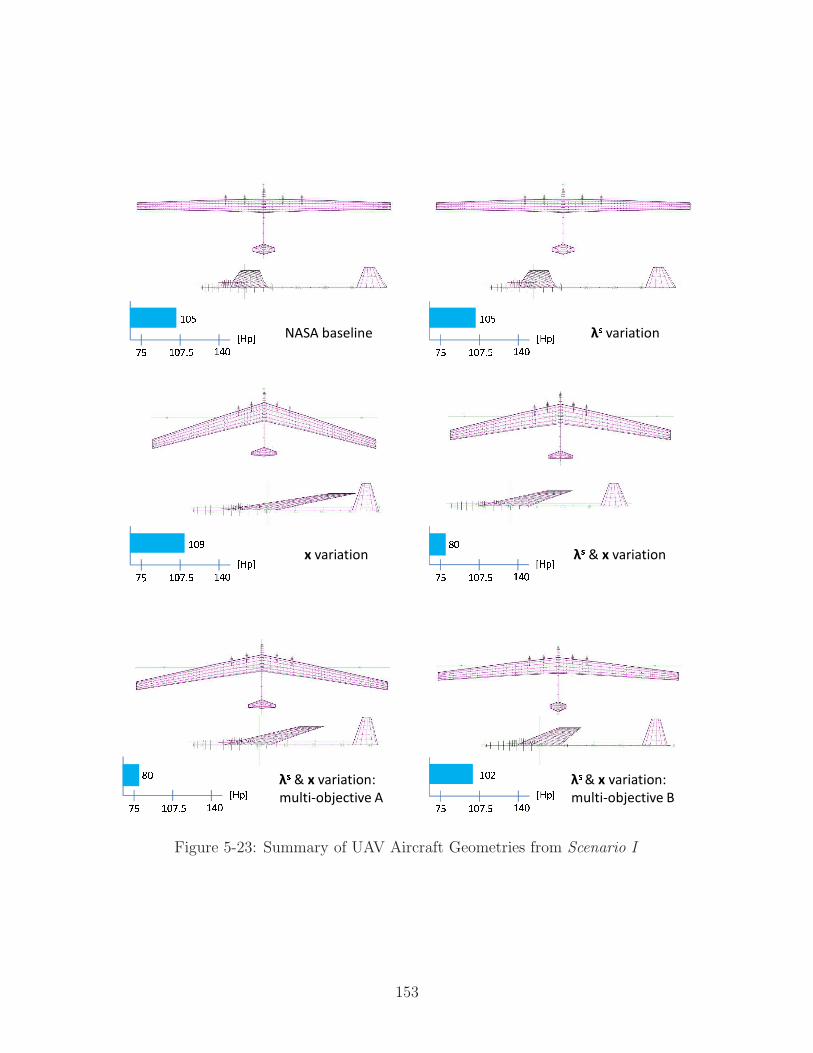
wx yz{y{w|x }~��y{x wx yz{y{w|x }~��y{x
�� �������� ������� �� �������� ������
�� �������� ������ wx yz{y{w|x }~��y{�
NASA baseline λ� variation
x variation λ� & x variation
λ� & x variation:multi-objective A
λ� & x variation:multi-objective B
Figure 5-23: Summary of UAV Aircraft Geometries from Scenario I
153
• Finally, examination of campaign level metrics derived from system level vehi-
cle performance demonstrated application of the methodology to systems with
shorter mission durations. Main effects of static design variables on these higher
level metrics showed unique trends that would not be found outside of the mul-
tistate analysis and design method. These include:
– The leveling out of the max engine power vs. campaign availability trend in
Fig. 5-19 near the high end of the power range. In a nominal state analysis
for endurance, this trend would continue its negative slope as increasing
engine size results in higher energy consumption and increasing mass.
– The concave shape of the wing sweep vs. sorties failed trend in Fig. 5-20.
In a nominal state analysis, best endurance would occur with zero wing
sweep and have a continuous negative slope towards the high end of the
wing sweep range.
– The constant negative slope of the max engine power vs. vehicles lost trend
in Fig. 5-22. For nominal endurance, the trend in max engine power would
have a positive slope (improve endurance) near the low end of the power
range, reach an optimum, and then have a continuously negative slope
(decrease endurance) as the max engine power increased.
Specific results of the Scenario I analysis showed that the combined multistate
approach demonstrated improvement in system availability of 11%, at a 3% lower cost,
when compared to the baseline aircraft designed for nominal performance. Variation
of component failure rates or static design variables alone showed improvement of
only 6.5%. Furthermore, when considering multiple objectives of system availability,
expected performance, nominal performance, and cost, the combined approach was
still able to achieve an 11% improvement in availability, with only a 4.5% decrease in
nominal performance, albeit at a small 6% increase in aircraft flyaway cost.
154
Chapter 6
Case Study - III: Lubrication
System for a Geared Turbofan
Engine
This chapter extends the methodology by demonstrating application of multistate
analysis and design to a lower level aerospace subsystem. The case study is the
lubrication system for a high bypass ratio geared turbofan (GTF) engine in the 20,000-
to 30,000-lbf thrust class. Whereas traditional turbofan engines have a fixed shaft
connecting the fan with the low-pressure turbine and compressor, the GTF engine
has a fan drive gear system that couples the fan to the low pressure spool, allowing
both the fan and the compressor to operate at more efficient wheel speeds. This has
advantages of improving fuel efficiency and reducing noise levels, but results in a more
complex and operationally critical lubrication system.
The lubrication subsystem is modeled for a single set of time-variant operational
parameters, representing the typical mission profile of an airline passenger jet. A
Pareto optimum solution is taken from the output space of expected oil temperature
versus cooling surface size. This serves as the baseline for sensitivity analysis and
improvement of expected availability via Pareto fronts calculated using the surrogate
function for EA. The goal of this case study is to quantify how specific changes
to the lubrication system’s design might improve the robustness of its performance
155

across several modes of failure, and to demonstrate the methodology such that it
may be extended to a more detailed multistate analysis given higher fidelity tools
and models available to engine industry experts. Results were favorable, showing
that when compared to the traditional, nominal case design as a baseline, performing
the multistate design analysis improves the overall lubrication system availability by
as much as 22% over a 500-hour maintenance interval.
6.1 The Geared Turbofan Engine Concept
The underlying principle of the GTF engine, shown in Fig. 6-1, is to further increase
bypass ratio over current designs in order to improve propulsive efficiency (specific fuel
consumption), decreasing noise and hopefully weight at the same time. The above
is achieved by reducing fan speed through a gearbox to allow higher low-pressure
compressor (LPC) and turbine (LPT) speeds and efficiencies. This generally leads to
a larger fan for the same thrust demand, where the final outcome is a high bypass
ratio turbofan engine with low thrust-specific-fuel-consumption (TSFC) and lower
specific thrust [71]. Along with the low bypass jet velocity comes low jet noise [88],
and because of the correspondingly slow fan speed, the fan emitted sound pressure
level is lower.
The geared turbofan engine concept has existed in smaller class turbofan engines
for several decades (e.g. Honeywell TFE731), where loading of the gear-box was kept
at relatively benign levels due to low thrust output. Only recently have improvements
in technology and materials made such gearing systems viable on high thrust engines
used by medium- and long-haul airliners such as the Boeing 777 or the Airbus A320.
Even so, many engine manufacturers remain reluctant to invest in the technology due
to perceived concerns about engine maintainability and system complexity, often on
the part of aircraft manufacturers or the airlines themselves. A recent study done at
MIT found that the integration of the fan drive gear system (FDGS) into the turbofan
engine does in fact drive a significant increase in complexity of supporting systems,
specifically on the performance and integration of the lubrication system [95].
156
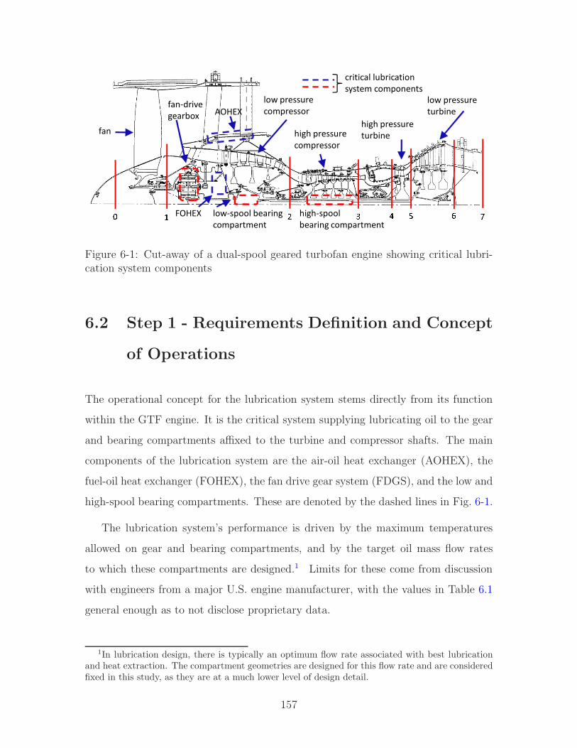
low pressureturbine
high pressureturbine
low pressurecompressor
high pressurecompressor
fan
fan-drivegearbox
� � � � � � � low-spool bearingcompartment
AOHEX
FOHEX high-spoolbearing compartment
critical lubrication system components
Figure 6-1: Cut-away of a dual-spool geared turbofan engine showing critical lubri-cation system components
6.2 Step 1 - Requirements Definition and Concept
of Operations
The operational concept for the lubrication system stems directly from its function
within the GTF engine. It is the critical system supplying lubricating oil to the gear
and bearing compartments affixed to the turbine and compressor shafts. The main
components of the lubrication system are the air-oil heat exchanger (AOHEX), the
fuel-oil heat exchanger (FOHEX), the fan drive gear system (FDGS), and the low and
high-spool bearing compartments. These are denoted by the dashed lines in Fig. 6-1.
The lubrication system’s performance is driven by the maximum temperatures
allowed on gear and bearing compartments, and by the target oil mass flow rates
to which these compartments are designed.1 Limits for these come from discussion
with engineers from a major U.S. engine manufacturer, with the values in Table 6.1
general enough as to not disclose proprietary data.
1In lubrication design, there is typically an optimum flow rate associated with best lubricationand heat extraction. The compartment geometries are designed for this flow rate and are consideredfixed in this study, as they are at a much lower level of design detail.
157
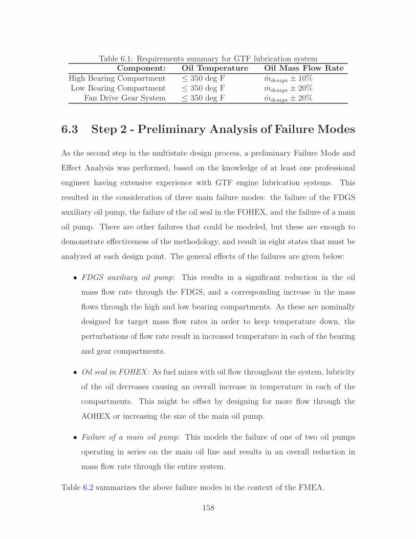
Table 6.1: Requirements summary for GTF lubrication systemComponent: Oil Temperature Oil Mass Flow Rate
High Bearing Compartment ≤ 350 deg F mdesign ± 10%Low Bearing Compartment ≤ 350 deg F mdesign ± 20%
Fan Drive Gear System ≤ 350 deg F mdesign ± 20%
6.3 Step 2 - Preliminary Analysis of Failure Modes
As the second step in the multistate design process, a preliminary Failure Mode and
Effect Analysis was performed, based on the knowledge of at least one professional
engineer having extensive experience with GTF engine lubrication systems. This
resulted in the consideration of three main failure modes: the failure of the FDGS
auxiliary oil pump, the failure of the oil seal in the FOHEX, and the failure of a main
oil pump. There are other failures that could be modeled, but these are enough to
demonstrate effectiveness of the methodology, and result in eight states that must be
analyzed at each design point. The general effects of the failures are given below:
• FDGS auxiliary oil pump: This results in a significant reduction in the oil
mass flow rate through the FDGS, and a corresponding increase in the mass
flows through the high and low bearing compartments. As these are nominally
designed for target mass flow rates in order to keep temperature down, the
perturbations of flow rate result in increased temperature in each of the bearing
and gear compartments.
• Oil seal in FOHEX : As fuel mixes with oil flow throughout the system, lubricity
of the oil decreases causing an overall increase in temperature in each of the
compartments. This might be offset by designing for more flow through the
AOHEX or increasing the size of the main oil pump.
• Failure of a main oil pump: This models the failure of one of two oil pumps
operating in series on the main oil line and results in an overall reduction in
mass flow rate through the entire system.
Table 6.2 summarizes the above failure modes in the context of the FMEA.
158

Table 6.2: Summary of preliminary FMEA for the GTF lubrication systemCom- Failure Failure
ponent Function Mode Effect Rate [1/hr] Mitigationmainline provide partial 50% press.
pump pressure inop loss 1/5000 n/aauxiliary provide FDGS press. increase
pump pressure inop loss 1/5000 FDGS flowFOHEX prevent fuel loss in increase
seal contamination leak lubricity 1/2500 AOHEX flow
The transition rate vector is λs = [λmain λaux λseal], denoting the respective
component failure rates shown in Table 6.2. These are taken from airline data on
aircraft maintenance planning found in Tozan, et al. [108]
6.4 Step 3 - System and Performance Classifica-
tion
Step 3 classifies the system according to its level of analysis, and determines whether
the performance metric is dynamic or static. The lubrication system study considers
only the lower, single system level, although an extension to multiple engine, phased
operation is conceivable. Performance output are the oil temperatures of the system
components, as well as the overall average system oil temperature. These temper-
atures are functions of the time-varying load on the engine and the corresponding
variations in oil mass flow throughout the system. Thus, the responses are dynamic
and the performance analysis accomplished through simulation, with an appropriate
controller in place to regulate oil flow through the FDGS. This is described further
in the following section.
6.5 Step 4 - Modeling and Simulation
The lubrication system, as shown in Fig. 6-2, was constructed in MATLAB’s Simscape R©software to as closely resemble a GTF engine’s oil system as possible. This was ac-
159
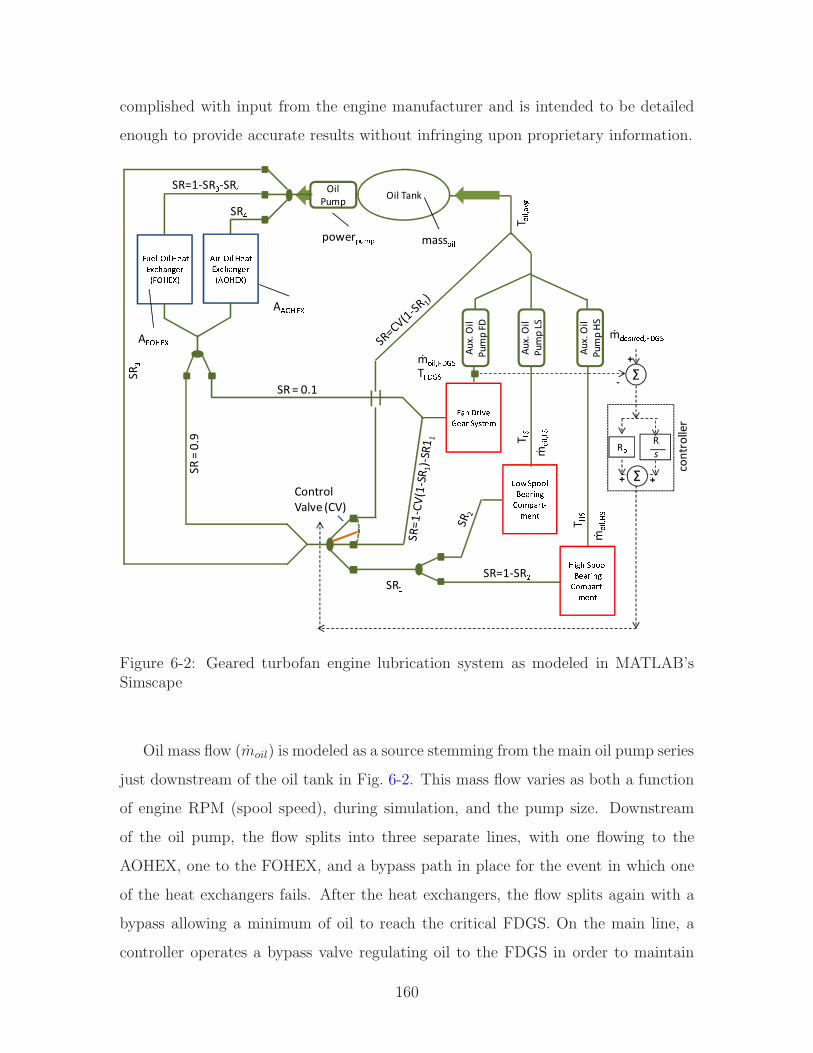
complished with input from the engine manufacturer and is intended to be detailed
enough to provide accurate results without infringing upon proprietary information.
¡¢£¤¥¢¢¦§¨©ª«¬®¢¯¥©ª°±¯¨¬° ²«³ ¤¥¢¢¦§¨©ª«¬®¢¯¥©ª°±¯¨¬°
´©¬ µª«¶¨·¨©ª ¤¸¹°¨¯
Oil Pump Oil Tankº«ª±»«¦ ²¨©°¼½¾³©¬¨ª¿º»²¼ÀÁ´Â¨¦±»«¦ ²¨©°¼½¾³©¬¨ª¿´»²¼ÀÁ
SRÃ
SR
ÄSRÅ
ControlValve (CV)
massÆÇÈpowerÉÊËÉ
ṁ
ÌÍÎ ÏÐÑṁ
ÌÍÎ ÏÒÑT
ÐÑT
ÒÑTÓÔÕÖTÌÍÎ Ï×ØÙ
AÚÛÜÝÞAÓÛÜÝÞ
Aux.
Oil
Pump
HS
Aux.
Oil
Pump
LS
Aux.
Oil
Pump
FD
SR=1-SRß-SRÅ
SR = 0.1
SR =
0.9
SR=1-SRà
ṁáâãÇäâáåÓÔÕÖΣ
+
-
Ræ Rçs
Σ ++
cont
rolle
r
ṁÆÇÈåÓÔÕÖ
Figure 6-2: Geared turbofan engine lubrication system as modeled in MATLAB’sSimscape
Oil mass flow (moil) is modeled as a source stemming from the main oil pump series
just downstream of the oil tank in Fig. 6-2. This mass flow varies as both a function
of engine RPM (spool speed), during simulation, and the pump size. Downstream
of the oil pump, the flow splits into three separate lines, with one flowing to the
AOHEX, one to the FOHEX, and a bypass path in place for the event in which one
of the heat exchangers fails. After the heat exchangers, the flow splits again with a
bypass allowing a minimum of oil to reach the critical FDGS. On the main line, a
controller operates a bypass valve regulating oil to the FDGS in order to maintain
160
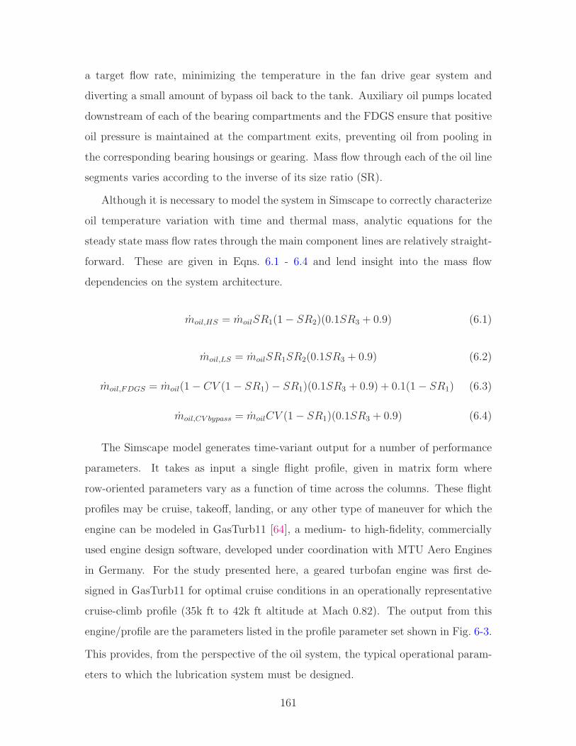
a target flow rate, minimizing the temperature in the fan drive gear system and
diverting a small amount of bypass oil back to the tank. Auxiliary oil pumps located
downstream of each of the bearing compartments and the FDGS ensure that positive
oil pressure is maintained at the compartment exits, preventing oil from pooling in
the corresponding bearing housings or gearing. Mass flow through each of the oil line
segments varies according to the inverse of its size ratio (SR).
Although it is necessary to model the system in Simscape to correctly characterize
oil temperature variation with time and thermal mass, analytic equations for the
steady state mass flow rates through the main component lines are relatively straight-
forward. These are given in Eqns. 6.1 - 6.4 and lend insight into the mass flow
dependencies on the system architecture.
moil,HS = moilSR1(1− SR2)(0.1SR3 + 0.9) (6.1)
moil,LS = moilSR1SR2(0.1SR3 + 0.9) (6.2)
moil,FDGS = moil(1− CV (1− SR1)− SR1)(0.1SR3 + 0.9) + 0.1(1− SR1) (6.3)
moil,CV bypass = moilCV (1− SR1)(0.1SR3 + 0.9) (6.4)
The Simscape model generates time-variant output for a number of performance
parameters. It takes as input a single flight profile, given in matrix form where
row-oriented parameters vary as a function of time across the columns. These flight
profiles may be cruise, takeoff, landing, or any other type of maneuver for which the
engine can be modeled in GasTurb11 [64], a medium- to high-fidelity, commercially
used engine design software, developed under coordination with MTU Aero Engines
in Germany. For the study presented here, a geared turbofan engine was first de-
signed in GasTurb11 for optimal cruise conditions in an operationally representative
cruise-climb profile (35k ft to 42k ft altitude at Mach 0.82). The output from this
engine/profile are the parameters listed in the profile parameter set shown in Fig. 6-3.
This provides, from the perspective of the oil system, the typical operational param-
eters to which the lubrication system must be designed.
161
35K ft.42K ft.
èéêëìééíîïðñòóôõéöìðñ÷øöïó÷ ùòôú ëìééíîïðñòóôõéöìðñ÷øöïó÷ûðóüñòýïþïðñ ëÿ�÷ïö������� � �� �� òñø�òíùïð÷���úðóôïñ���ù���û�ïíø�òíùïð÷���úðóôïñ�û�ù���
������ ���
� !"# $%&$'( )�%*+&,,-./0 1(#2342
5678 9:;5678 9<; =:;=<;>?@AB =678 9CDEFGHIJKF?HIJK LMNOPQR SMTUVWLMNOPQR SMTUXWLMNOPQR SMTUYZ��[\]�� ]�����[ _`\��abcd ��[\]��e
fghi.jhgk?@ABlmnop oqrl ss tuvwxuyyzxf-./k?@AB
M=0.82
c=[RPM{|,RPM}|,RPM~��,τ~��|���,…ṁ���,T���, ṁ����,T����]���profile parameter set, f(t)
m���A~�{��A��{��
SR�SR�SR�SR�
P��������T�������
T����~��|T����{|�T����}|�S{���de
sign v
ector
, x Output Vector
Optimizer
lubricationsystem
Figure 6-3: Baseline (nominal) optimization flow
The baseline nominal case optimization follows the flow depicted in Fig. 6-3, where
Eqn. 6.5 shows the formal, single objective optimization problem:
given parameter set, c, controller gains, r
c = [RPMHS, RPMLS, RPMFAN , τFDGS,in, mair, Tair, mfuel, Tfuel]t
r = [Rp, Ri]
minimize J(x, r, c) = Toil,avg(x, r, c)
x = [moil, AAOHEX , AFOHEX, SR1, SR2, SR3, SR4, Ppump]
s.t. xi,LB ≤ xi ≤ xi,UB, i = 1, 2, ..., 8
(6.5)
The multistate problem is significantly more complex in construction and execution,
namely because the lubrication system analysis must be executed for several failed
modes of operation in addition to the nominal case. A description of this setup is
given in the next section.
The oil system presents a meaningful design problem involving trade-offs between
the lubrication and temperature requirements of each of the bearing compartments
162

and the FDGS, the size of the air and fuel heat exchangers required to maintain
operating oil temperature, and the oil flow rate supplied by the engine and oil pump.
The bearing and gear compartments are typically designed to specifications that result
in a minimum operating temperature occurring at a specific oil mass flow rate. Thus
the overall system must provide these target flow rates, which are different for each of
the components, while at the same time managing flow rates to the air and oil heat
exchangers in order to maximize heat extraction.
6.6 Step 5 - Markov Analysis
A good description of the general multistate problem setup and Markov analysis is
found Chapters 3, 4, and 5, therefore the following focuses on the multistate formu-
lation issues specific to the GTF lubrication system.
Given that the state performances, GsK , do not depend on the order of failure, the
symmetric Markov chain requires only eight states, as shown in Fig. 6-4.
N 2 5
4
7
6
1
3
λ����λ� ¡λ¢£�¤ λ����
λ����λ¢£�¤
λ¢£�¤λ����λ¢£�¤λ� ¡λ� ¡
λ� ¡[G¢¥,P¢¥] [G¢¦,P¢¦]
[G¢§,P¢§][G¢,P¢]
[G¢©,P¢©][G¢ª,P¢ª][G¢«,P¢«]
[G¢¬,P¢¬]Figure 6-4: GTF lubrication system Markov formulation
The solution to the above chain yields the state probabilities, P sK,1,..,7, correspond-
ing to the nominal state, N, and each of the failed states, 1 through 7. The probability
set, Ps, and state performance set, Gs, are computed at each iteration in the multi-
state optimization process shown in Fig. 6-5.
163

®¯°±®®²³´µ¶·¸¹º®»±µ¶¼½»´¸¼ ¾·¹¿ °±®®²³´µ¶·¸¹º®»±µ¶¼½» ¸¼Àµ¸Á¶·Â´Ã´µ¶ °Äż´»ÆÇÈÉÊËÌ ÍÎÏ ÐÑÒÓÔ·¶½Õ·² ¾´µ¼Ö×Ø¿µ¸¹ ¶ÙÔÕ¾ÖÚÛÀÜ´²½Õ· ²¾´µ¼Ö×Ø¿µ ¹´¶ÙÀÕ¾ÖÚÛ ÝÞßàáâ ÝÞã äåæçèåéêëéìíîäêï ðëññòó ôõåöíè÷øù÷ úûüý þÿ�úûüý þ�� �ÿ��������� �ûüý þ��� ����� ��� ������� ������������� ������������� ������ÝÞ !"ÝÞ#"ÝÞã ÝÞ $%!àá&'() ÝÞ !"ÝÞ* +,-.ó/-,0����12345 4671 88 9:;<=:>>?=+òóô0����c=[RPM@A,RPMBA,RPMCD E,τCFGAHIJ,…
ṁKIL,TKIL, ṁMNOP,TMNOP]QRSprofile parameter set, f(t)
mTIPACU@VWADU@VW
SRSSRXSRYSRZ
PTIP[\N]\λmainλauxλseal
E[TTIPHK^_]E[TTIPHCFGA ]E[TTIPH@A` ]E[TTIPHBA` ]
desig
n vec
tor, x
, λS output vector
Optimizerlubrication system a b cd efghijklmiknoipqkrst susv swsx syijklm ijklmipqkr ipqkrijklmipqkriknoikno ikno
Markov solver
Gz{state,K
Figure 6-5: GTF multistate optimization flow
Equation 6.6 gives the formal multistate optimization statement:
given parameter set, c, controller gains, r
c = [RPMHS, RPMLS, RPMFAN , τFDGS,in, mair, Tair, mfuel, Tfuel]t
r = [Rp, Ri]
minimize −EG(x,λs, r, c) = −
7∑
K=N
P sK(λ
s)Toil,avg,K(x, r, c) or
− SEA(x,λs, r, c) = −
7∑
K=N
P sK(λ
s){ b
b(max[1+(350−TK (x,r,c)),1])}
x = [moil, AAOHEX , AFOHEX, SR1, SR2, SR3, SR4, Ppump]
λs = [λmain, λaux, λseal]
s.t. xi,LB ≤ xi ≤ xi,UB, i = 1, 2, ..., 8
λsi,LB ≤ λsi ≤ λsi,UB, i = 1, 2, 3
(6.6)
In Chapter 5, a cost was associated with increasing the MTBF of any particu-
lar component, and this was incorporated into the overall UAV system cost model.
For the lubrication system study, however, the cost model was not readily available
164

(although it is generally available to the manufacturer). The result is that including
the component failure rates as variables in Eqn. 6.6 above will nearly always result
in failure rates being driven to their lower limits. Nevertheless, these variables were
included in the sensitivity analyses of Section 6.7.1, which allows direct comparison
between failure rate driven sensitivities and those driven by the static design variables,
even in the absence of cost.
6.7 Step 6 - Analysis and Visualization of Results
Step 6 presents the results according to a logical process intended to highlight the
differences between the traditional, nominal design solution and the multistate solu-
tion. First, a Pareto optimal solution for the nominal case is taken from the Pareto
front in Fig. 6-9 (this chart will be described further at the end of the section). This
is chosen as Point 5 from the nominal front, which occurs just before further in-
creases in heat exchanger size become ineffective in reducing system oil temperature.
Next, this point is examined in Figs. 6-6, 6-7, and 6-8, from a multistate perspec-
tive, to illustrate the behavior of performance and sensitivities under the influence of
numerous failure states. Finally, Pareto fronts are constructed using the multistate
system expected performance and availability for time periods of 100- and 500-hrs
respectively, time periods which might be experienced between instances of scheduled
maintenance on various geared turbofan engines. The final results demonstrate sig-
nificant improvement in expected availability between the nominal case design point
and the multistate design points.
The important design variables, x, for the lubrication system shown in Fig. 6-2,
are given in Table 6.3 along with the upper and lower limits used in the design
optimization described in the next section. Output of the analysis is the average oil
temperature, the temperature of the oil in the bearing compartments and the FDGS,
and the size of the air and fuel heat exchangers.
In this case study, the number of states is low enough to individually observe the
outputs of GsK for several different design perturbations. This provides insight into
165

Table 6.3: Lubrication system design variablesDesign moil AAOHEX AFOHEX SR1 SR2 SR3 SR4 Ppump
Variables [kg] [m2] [m2] [nd] [nd] [nd] [nd] [kW]xlb 50 0.5 0.5 0.35 0.1 0.05 0.05 0.3
xinit 55 1 1 0.5 0.5 0.2 0.55 1xub 60 1.3 1.3 0.95 0.8 0.9 0.8 1.5
how the performance thresholds interact with design changes on a state-specific basis,
as shown through the quad-plots of Fig. 6-6.
Each quadrant of the plot is a representation of two critical system temperatures.
These are chosen from the system average oil temperature, Tavg, high bearing oil
temperature, Thb, low bearing temperature, Tlb, and the fan drive gear system tem-
perature, Tfdgs. The pairing of temperatures in each quadrant is for purposes of
illustration, helping to spread out the points along two axes instead of one, with-
out affecting temperature magnitude representation. Note that the scales in each
quadrant are increasing positive outward from 200 to 500 degrees Fahrenheit.
In each quadrant are 17 design points, made by taking the nominal design point
as baseline and perturbing each of the eight design variables in Table 6.3 by ± 10%.
The blue dashed lines are the location of the nominal design point. The red dashed
lines indicate the operationally critical temperature of 350 deg F.
As one would hope, in the nominal state, the baseline design as well as each of the
perturbed designs is located well within the safe region for each of the temperature
metrics. In the case of State 1, however, the baseline design remains under limits
for the FDGS, low bearing, and average system oil temperatures, but far exceeds
the limit for the high bearing temperature. This is due to the fact that the high
bearing oil temperature is much more sensitive to reductions in oil flow than the
other components.
Also of interest is that some of the designs in the upper right quadrant of State
1 span the critical temperature limit for Tavg . This indicates an area where small
changes to design variables other than component failure rates can affect the system’s
availability, which depends on the crossing of a performance limit threshold. In the
case of State 1, these changes promote a crossing from the baseline to an unsafe area
166
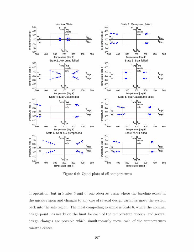
500 400 300 200 300 400 500500
400
300
200
300
400
500
Temperature [deg F]
Tem
pera
ture
[de
g F
]
Nominal State
unsafe
safe
Tavg
Tlb
Tavg
Tlb
Thb Tfdgs
ThbTfdgs
500 400 300 200 300 400 500500
400
300
200
300
400
500
Temperature [deg F]
Tem
pera
ture
[de
g F
]
State 1: Main pump failed
unsafe
safe
Tavg
Tlb
Tavg
Tlb
Thb Tfdgs
ThbTfdgs
500 400 300 200 300 400 500500
400
300
200
300
400
500
Temperature [deg F]
Tem
pera
ture
[de
g F
]
State 2: Aux pump failed
unsafe
safe
Tavg
Tlb
Tavg
Tlb
Thb Tfdgs
ThbTfdgs
500 400 300 200 300 400 500500
400
300
200
300
400
500
Temperature [deg F]
Tem
pera
ture
[de
g F
]
State 3: Seal failed
unsafe
safe
Tavg
Tlb
Tavg
Tlb
Thb Tfdgs
ThbTfdgs
500 400 300 200 300 400 500500
400
300
200
300
400
500
Temperature [deg F]
Tem
pera
ture
[de
g F
]
State 4: Main, seal failed
unsafe
safe
Tavg
Tlb
Tavg
Tlb
Thb Tfdgs
ThbTfdgs
500 400 300 200 300 400 500500
400
300
200
300
400
500
Temperature [deg F]
Tem
pera
ture
[de
g F
]
State 5: Main, aux pump failed
unsafe
safe
Tavg
Tlb
Tavg
Tlb
Thb Tfdgs
ThbTfdgs
500 400 300 200 300 400 500500
400
300
200
300
400
500
Temperature [deg F]
Tem
pera
ture
[de
g F
]
State 6: Seal, aux pump failed
unsafe
safe
Tavg
Tlb
Tavg
Tlb
Thb Tfdgs
ThbTfdgs
500 400 300 200 300 400 500500
400
300
200
300
400
500
Temperature [deg F]
Tem
pera
ture
[de
g F
]
State 7: All Failed
unsafe
safe
Tavg
Tlb
Tavg
Tlb
Thb Tfdgs
ThbTfdgs
Figure 6-6: Quad-plots of oil temperatures
of operation, but in States 5 and 6, one observes cases where the baseline exists in
the unsafe region and changes to any one of several design variables move the system
back into the safe region. The most compelling example is State 6, where the nominal
design point lies nearly on the limit for each of the temperature criteria, and several
design changes are possible which simultaneously move each of the temperatures
towards center.
167
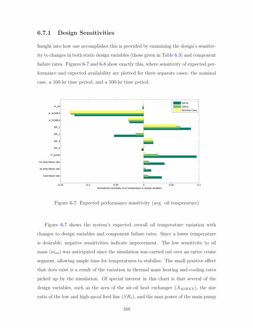
6.7.1 Design Sensitivities
Insight into how one accomplishes this is provided by examining the design’s sensitiv-
ity to changes in both static design variables (those given in Table 6.3) and component
failure rates. Figures 6-7 and 6-8 show exactly this, where sensitivity of expected per-
formance and expected availability are plotted for three separate cases: the nominal
case, a 100-hr time period, and a 500-hr time period.
-0.15 -0.1 -0.05 0 0.05 0.1
seal failure rate
ax pmp failure rate
mn pmp failure rate
P_pump
SR_4
SR_3
SR_2
SR_1
A_FOHEX
A_AOHEX
m_oil
Normalized sensitivity of oil temperature to design variables
500-hr
100-hr
Nominal Case
Figure 6-7: Expected performance sensitivity (avg. oil temperature)
Figure 6-7 shows the system’s expected overall oil temperature variation with
changes to design variables and component failure rates. Since a lower temperature
is desirable, negative sensitivities indicate improvement. The low sensitivity to oil
mass (moil) was anticipated since the simulation was carried out over an entire cruise
segment, allowing ample time for temperatures to stabilize. The small positive effect
that does exist is a result of the variation in thermal mass heating and cooling rates
picked up by the simulation. Of special interest in this chart is that several of the
design variables, such as the area of the air-oil heat exchanger (AAOHEX), the size
ratio of the low and high-spool feed line (SR1), and the max power of the main pump
168
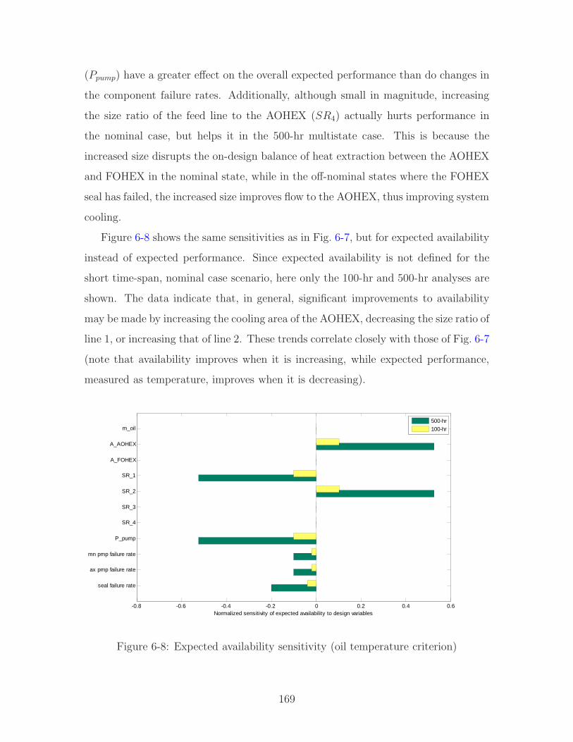
(Ppump) have a greater effect on the overall expected performance than do changes in
the component failure rates. Additionally, although small in magnitude, increasing
the size ratio of the feed line to the AOHEX (SR4) actually hurts performance in
the nominal case, but helps it in the 500-hr multistate case. This is because the
increased size disrupts the on-design balance of heat extraction between the AOHEX
and FOHEX in the nominal state, while in the off-nominal states where the FOHEX
seal has failed, the increased size improves flow to the AOHEX, thus improving system
cooling.
Figure 6-8 shows the same sensitivities as in Fig. 6-7, but for expected availability
instead of expected performance. Since expected availability is not defined for the
short time-span, nominal case scenario, here only the 100-hr and 500-hr analyses are
shown. The data indicate that, in general, significant improvements to availability
may be made by increasing the cooling area of the AOHEX, decreasing the size ratio of
line 1, or increasing that of line 2. These trends correlate closely with those of Fig. 6-7
(note that availability improves when it is increasing, while expected performance,
measured as temperature, improves when it is decreasing).
-0.8 -0.6 -0.4 -0.2 0 0.2 0.4 0.6
seal failure rate
ax pmp failure rate
mn pmp failure rate
P_pump
SR_4
SR_3
SR_2
SR_1
A_FOHEX
A_AOHEX
m_oil
Normalized sensitivity of expected availability to design variables
500-hr
100-hr
Figure 6-8: Expected availability sensitivity (oil temperature criterion)
169
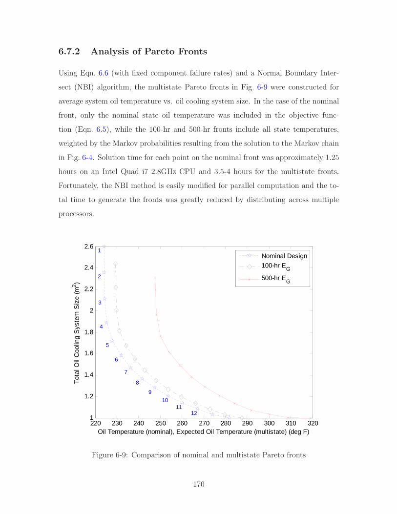
6.7.2 Analysis of Pareto Fronts
Using Eqn. 6.6 (with fixed component failure rates) and a Normal Boundary Inter-
sect (NBI) algorithm, the multistate Pareto fronts in Fig. 6-9 were constructed for
average system oil temperature vs. oil cooling system size. In the case of the nominal
front, only the nominal state oil temperature was included in the objective func-
tion (Eqn. 6.5), while the 100-hr and 500-hr fronts include all state temperatures,
weighted by the Markov probabilities resulting from the solution to the Markov chain
in Fig. 6-4. Solution time for each point on the nominal front was approximately 1.25
hours on an Intel Quad i7 2.8GHz CPU and 3.5-4 hours for the multistate fronts.
Fortunately, the NBI method is easily modified for parallel computation and the to-
tal time to generate the fronts was greatly reduced by distributing across multiple
processors.
220 230 240 250 260 270 280 290 300 310 3201
1.2
1.4
1.6
1.8
2
2.2
2.4
2.6
Oil Temperature (nominal), Expected Oil Temperature (multistate) (deg F)
Tot
al O
il C
oolin
g S
yste
m S
ize
(m2 )
1
2
3
4
5
6
7
8
9
1011
12
Nominal Design
100-hr EG
500-hr EG
Figure 6-9: Comparison of nominal and multistate Pareto fronts
170

As expected, the two multistate fronts shift to the right, due to the inclusion of
the failure states that have higher temperatures and higher probability of occurring
as the period of time increases. However, measurable improvement is realized when
comparing the expected availability of the best design point taken from the nominal
front (Point 5) to those of the best multistate designs, as shown in Fig. 6-10. Point
5, analyzed for the 100-hr time period, has E100A,N=0.923, while the 100-hr multistate
design is 2% better with an availability of 0.942. The percent gain for the 500-hr
analyses is even larger, at 10%. These are significant improvements, considering that
they do not include the effect of decreasing component failure rates and were achieved
merely by affecting the system’s architectural design.
E|}~���= .923
E|}~���= .67
E|}��������= .942
E|}��������= .74
Figure 6-10: Blow-up of expected performance Pareto fronts showing improvementin expected availability
The sensitivity plots in Figs. 6-7 and 6-8 indicated that availability and expected
performance were positively correlated for the lubrication system study. To deter-
mine whether further improvements to EA were possible, Pareto fronts for system
availability vs. oil cooling system size were constructed using the NBI algorithm with
the surrogate function for availability, SEA. Figure 6-11 shows results for these Pareto
fronts, along with the exact values of availability for each design point.
Unlike the Pareto front estimations shown for the UAV case study in Fig. 5-13,
of Chapter 5, Fig. 6-11 shows the lubrication system availability breaking into three
171
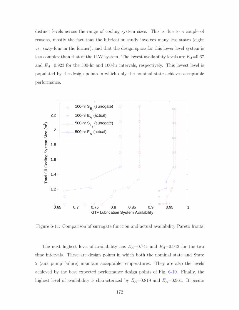
distinct levels across the range of cooling system sizes. This is due to a couple of
reasons, mostly the fact that the lubrication study involves many less states (eight
vs. sixty-four in the former), and that the design space for this lower level system is
less complex than that of the UAV system. The lowest availability levels are EA=0.67
and EA=0.923 for the 500-hr and 100-hr intervals, respectively. This lowest level is
populated by the design points in which only the nominal state achieves acceptable
performance.
0.65 0.7 0.75 0.8 0.85 0.9 0.95 11
1.2
1.4
1.6
1.8
2
2.2
GTF Lubrication System Availability
Tot
al O
il C
oolin
g S
yste
m S
ize
(m2 )
100-hr SE
A
(surrogate)
100-hr EA
(actual)
500-hr SEA
(surrogate)
500-hr EA
(actual)
Figure 6-11: Comparison of surrogate function and actual availability Pareto fronts
The next highest level of availability has EA=0.741 and EA=0.942 for the two
time intervals. These are design points in which both the nominal state and State
2 (aux pump failure) maintain acceptable temperatures. They are also the levels
achieved by the best expected performance design points of Fig. 6-10. Finally, the
highest level of availability is characterized by EA=0.819 and EA=0.961. It occurs
172

as State 2 leaves the acceptable set and State 3 (FOHEX seal failure) enters (note
that P s3 > P s
2 ). These values of availability represent improvements of 22.2% for the
500-hr case, and 4.1% for the 100-hr case, when compared to the values of availability
resulting from the nominal design optimization.
In general, the surrogate function for availability satisfactorily modeled the trends
for actual availability. The smoothing term base (see Eqn.6.6) was b=10 for the 500-hr
interval and b=50 for the 100-hr interval, as these were determined through exper-
imentation to provide the best results. The 100-hr interval required less smoothing
than did the 500-hr interval because the degree of change between availability lev-
els was much smaller. The different bases are also evident in the difference between
magnitudes of actual and surrogate results for each respective time interval. In both
cases, however, the trends in exact availability are in agreement.
Finally, the Normal Boundary Intersect (NBI) method for Pareto front determi-
nation is very unforgiving in regions where the front is concave. Therefore, some of
the convergence criteria were relaxed on the point optimizations in order to prevent
extraordinarily long run times. The point spacing on the SEAfronts are somewhat
less than uniform in certain areas as a result. This did not significantly affect the EA
fronts. In fact, some of the points on the front for exact availability would not have
been found without the smoothing provided by the surrogate function.2
6.8 Case Summary
This chapter applied multistate analysis and design to the lubrication system of a
geared turbofan engine. Where previous case studies demonstrated the methodol-
ogy on higher level aircraft systems, this study focused on a lower level subsystem,
demonstrating that, even with a less complex design space and fewer states, significant
improvements can be made to the subsystem’s availability through static design vari-
ables alone. Additionally, shorter analysis times allowed computation of full Pareto
2The points that would not have been found are the ones lying to the left of a straight line drawnbetween the points for maximum and minimum cooling system size, as the NBI algorithm [33] onlysearches in a direction of combined improvement w.r.t. (to the right of) the intersect line.
173
fronts for expected availability using the surrogate function introduced in Chapter 4.
The following points summarize key findings from this case study:
• Even in the simpler design space characterized by the lubrication subsystem,
sensitivity of expected performance to changes in static design variables varied
significantly between the nominal case and two multistate scenarios of differing
time duration (Fig. 6-7). In one case, the sign of the sensitivity even reverses
trend. The impact of this is that, designing for best performance in the nominal
scenario, while affecting availability only through component failure rates, will
likely result in an inferior multistate design.
• The surrogate function for availability, SEA, proved effective within a gradient-
based algorithm for generation of Pareto fronts. Although convergence in some
areas of the approximated front led to very long optimization times, the function
was still able to generate an accurate representation of the Pareto front for actual
availability.
• Variation of static design variables alone led to improvement of subsystem avail-
ability by 22% over a time duration of 500-hrs (Fig. 6-11). When considering
oil system cooling size as a representation of cost, and adjusting accordingly,
the best Pareto solution still resulted in an improvement of 10%. These gains
are promising and suggest that further analysis with a more detailed model for
cost and performance would be beneficial to the engine manufacturer.
174

Chapter 7
Conclusions
This final chapter begins by summarizing key results of the thesis. It draws together
major findings and conclusions arising from the three central case studies, and uses
these to develop some general principles for early-phase multistate analysis and design.
Finally, areas for future research are suggested, with a short summary of progress-to-
date in those directions.
7.1 Summary
The thesis lays a foundation for the in-depth and comprehensive exploration of com-
plex, multistate, early-phase design spaces. Advances in design optimization, comput-
ing power (including parallel processing), and certain reliability analysis techniques
enable this endeavor, whereas in the past it has remained prohibitively challenging.
The research integrates, refines, and tests these methodologies on several case studies
with high-dimensional performance state spaces.
The first chapter presents the compelling argument that, given current levels of
technology in component reliability, operators must accept the fact that ultra long
endurance systems, as demonstrated in Fig. 1-1, will likely not remain in their nominal
state of operation throughout their service duration. Thus, design practices that focus
on this state, even in the earliest phases, will result in suboptimal systems. This is
verified through results in all three case studies, including the design sensitivities of
175

Fig. 3-10 and Fig. 6-7, for the twin-engine aircraft and geared turbofan engine, and
most dramatically through Fig. 5-11, for the ultra long endurance UAV.
With the above motivation, Chapter 2 further develops the case for including
effects of static design variables, component failure rates, and control variables in the
multistate design loop. It defines multistate in the context of the present research,
placing scope within the appropriate rung of an extended hierarchy of system state
change (Fig. 2-6). This hierarchy sets the bounds on all possible considerations of
state within the context of system design, encompassing the search space potentially
achievable as design technology and computational ability advance.
The twin-engine aircraft study in Chapter 3 takes the first step into this search
space, demonstrating that the multistate performance behavior of a well-known and
validated aircraft system clearly exhibits itself in design sensitivities driven by both
static design variables and component failure rates. The performance model devel-
oped for the study is non-trivial and of significant fidelity, including elements for
dynamic control of the aircraft system at each design point. It has been developed
from simulation algorithms over ten years in the making [18] (see Appendix A), and
subsequently validated by real world flight test data. Results from this first case
study have also been recommended for publication in [1].
The lessons and experience gained from above are used to develop a generalized
methodology for multistate analysis and design in the fourth chapter (Fig. 4-1). The
methodology begins by identifying a broadened set of multistate requirements early
in the design process and performing a preliminary analysis of failure modes to define
the state transition rate vector, λs, in advance of multistate computational analysis.
Computational analysis then departs from traditional methods by integrating Markov
state analysis directly into the design loop. This includes processes for determining
multistate output as a function of static design variables, x, component failure rates,
λs, and controller gains, r, depending on the dynamics of the performance metric.
The output of this is often a multi-objective performance space, defined by expected
performance, nominal performance, system availability, and cost. The final step of
the methodology outlines several techniques for visualizing this performance output
176

space, all of which are demonstrated throughout the thesis case studies. The above
framework involves use of several tools from Multidisciplinary Design Analysis and
Optimization (MDAO), as well as the thesis developed supporting methods of multi-
layer Markov analysis and a surrogate function for system availability (both of which
are described in the last sections of Chapter 4). Figure 7-1 maps the use of these
techniques to the thesis case studies.
Case Study I
Case Study II.a
Case Study III
Twin-engine aircraft
Ultra-long endurance UAV(Scenario I)
GTF engine lubrication system
Point Design SensitivityAnalysis
DOE: Orthogonal Arrays
DOE: Latin-hypercube Spacing
DOE: Global Analysis of Main Effects
Constrained Gradient-based Optimization
Visual Presentation of Performance Output Space
Pareto Front Estimation
Pareto Front Calculation through Optimization
Dynamic Performance Model
Static Performance Model
Multilayer Markov Analysis
Surrogate Availability, S��
Analyzing
Visualizing
Analyzing
Visualizing
Analyzing
Visualizing
Case Study II.bLong endurance UAV in campaign(Scenario II)
Analyzing
Visualizing
Figure 7-1: Object-Process Diagram mapping of methods and techniques to caseapplications, double borders indicate supporting objects developed in thesis
The fifth chapter introduces the long endurance UAV case study, broken into its
two scenarios in Fig. 7-1 for ease of depiction. Scenario I of this case is an ultra long
177

endurance UAV with a mission duration of three months aloft. Here, a full analysis
of the DOE sampled design space for differing combinations of independent variables
shows clear distinction between each of the performance output spaces arising from: a)
component failure rate variation, b) static design variable variation, and c) combined
variation of both. The overlay plot in Fig. 5-13 portrays this best, depicting a region
of improved performance resulting from c), above, that is unachievable through either
a) or b). Scenario II is the case of a one-to-two day duration vehicle, involved in
a 5-year multi-sortie campaign requiring omnipresence over the mission area. This
scenario makes use of the multilayer Markov analysis technique to extend vehicle
level performance metrics to the campaign level. The design space is systematically
sampled via an orthogonal array and main effects of aircraft design variables on
attrition and sortie abort rates are plotted, showing an observable and measurable
link between the two.
Finally, Chapter 6 moves from the higher aircraft system level down to the lubri-
cation subsystem of a geared turbofan engine. The multistate methodology proves
effective on this lower level system as well, taking advantage of the computationally
cheaper performance analysis to broadly demonstrate use of the surrogate availability
function, SEA, across a range of gradient-based optimizations. While results of this
study showed less of a trade-off between expected performance and availability, due
to the simpler interaction between failure states, these metrics were still more sensi-
tive to changes in many of the static design variables than they were to changes in
component failure rates (Fig 6-7 and Fig. 6-8). Additionally, when compared to the
nominal case design, significant improvement in subsystem availability was realized
through variation of static design variables alone.
To conclude the thesis summary, the contributions of this research are outlined
below:
• The central multistate analysis and design methodology. This includes
the novel integration of Markov state analysis into the early-phase design loop
as shown in Fig. 4-1, of Chapter 4. Initial feasibility of the methodology is
demonstrated in Chapter 3, and it is successfully applied in Chapters 5 and 6.
178
• Demonstration of the cost and benefits, in the form of design trade-
offs, associated with a multistate design approach as compared to
pure reliability analysis or the nominal design approach. This is most
clearly shown in the results of Chapter 5, Fig. 5-13 and Tables 5.4, 5.5, and 5.6.
It is also observable in the design sensitivities of case studies in Chapter 3 and
Chapter 6.
• A multilayer approach, using Markov analysis, for translating sin-
gle sortie vehicle level metrics into measures of multistate campaign
performance. The process for multilayer Markov analysis is described in Sec-
tion 4.2.1, of Chapter 4, including a detailed example problem. It is applied
in Section 5.6.2, of Chapter 5. Data linking vehicle static design variables to
campaign level metrics for attrition, failed sorties, and availability are found in
Figs. 5-19 through 5-22.
• A surrogate function for system availability that allows the otherwise
piecewise-constant metric to be optimized via gradient-based opti-
mization algorithms. The function is first introduced in Section 4.2.2, of
Chapter 4. It is successfully used in Chapter 5 in the constrained gradient-
based optimization of Eqn. 5.5, with results in Fig. 5-15. It is again used in
Chapter 6 to generate the Pareto fronts of Fig. 6-11.
7.2 Major Findings and General Principles in Mul-
tistate Analysis and Design
The above section highlighted three central case studies: the twin-engine aircraft
(Chapter 3), the long endurance UAV (Chapter 5), and the geared turbofan engine
lubrication system (Chapter 6). This section focuses in more detail on the major
findings from those case studies, some of which are evident from the results, and
others which were more implicitly evident through the process of examination itself.
Several general principles are then suggested for consideration in future multistate
179

analysis and design endeavors.
The major findings, in order of what the author considers most significant to least
significant, are given below:
1. Each of the output spaces for the ultra long endurance UAV system availability
had distinctly unique shapes and boundaries, depending on whether they were
formed by: a) component failure rate variation, b) static design variable varia-
tion, or c) combined variation of both. The availability obtained by variation of
both was unachievable through variation of either independently. Those solu-
tions generated via component failure rates came at the expense of higher cost
with no effect on nominal performance, while those generated via static design
variables came at the expense of lower nominal performance with much lower
overall cost. The combined design space struck a balance between the two and
significantly extended the increase in system availability.
2. Results from all three case studies showed that small changes in static design
variables may be used to improve system availability and expected performance.
Furthermore, these sensitivities were quantifiable. In the case of the twin-engine
aircraft, the shifts were a result of improvement in stability and control char-
acteristics brought about by a larger control surface. With the UAV, there was
broad improvement across numerous states resulting from the lower required
trim moments of a slightly increased wing sweep. The lubrication system so-
lution achieved improvement by increasing the size ratio of an oil line that
improved cooling in the most likely failure state.
3. In general, there were competing objectives between system availability and nom-
inal performance, and to a lesser degree between system availability and expected
performance. This is shown most directly through the Pareto front estima-
tions in the UAV case study, with emphasis on the fact that the nominally de-
signed aircraft was characterized by a design point lying extreme opposite of the
non-dominated Pareto points for maximum system availability. The competing
trend between system availability and expected performance was much weaker
180
in the lubrication system study, noting that the best choice for expected perfor-
mance was also near the best choice for system availability. This is explained
by the following. To a certain degree, availability and expected performance
will rise together, as both attempt to better distribute performance, GsK , across
their weighted objective formulations. As more and more state thresholds, W ,
are crossed, however, expected performance continues to push all GsK up, while
availability only pushes those GsK up that have not achieved W . Thus, a highly
optimized availability will pull the extra few percent of improvement from the
performance surpluses of states in the acceptable set, thus decreasing expected
performance. In the case of the simpler lubrication system, there were many less
surpluses to be exploited than in the more complex UAV case. This emphasizes
the importance of performing a multi-objective analysis for systems in which
both performance and availability are important.
4. The extension of Markov analysis to the campaign level in the UAV study showed
a clear relationship between vehicle static design variables and the higher level
metrics of sorties failed and lost. Many of these showed unique trends arising
not only from vehicle performance behavior, but also from the passage of states
between the varying degrees of acceptance categories. The same wing sweep
effect described in Finding #2 was also observed here.
5. The surrogate function for system availability was effective in guiding the path
towards improved EA, even when the actual and surrogate values of availability
were not in close agreement. In the UAV case study, this function was used
to improve availability from an initial design point that was already quite close
to the final solution. The required smoothing was minimal and the surrogate
approximation value was nearly equal to that of the actual value. In the lu-
brication system study, the function was used across a broader Pareto front,
requiring much more smoothing. As a result, the surrogate value was signif-
icantly higher than the actual value. The exact Pareto front, however, was
accurate. Since the function is intended to model the shape of the availability
181

output space, and not its value, this behavior is expected. In fact, the value of
surrogate availability should always be higher than exact availability, in all but
the case where exact availability is equal to 1.0. This is because the surrogate
function includes within its summation a fraction of every state’s performance
deficiency, while the exact availability function does not (see Eqn. 4.12 and
Fig. 4-9 in Chapter 4).
The above findings assist in developing some general principles concerning mul-
tistate analysis and design in the early-phase development of complex systems. The
first of these relates to the issue of trade-offs discussed in Finding #3, and is succinctly
stated as:
The general multistate problem is also a multi-objective one
with competing trade-offs between nominal performance, system
availability, expected performance, and cost.
The degree of these trade-offs will depend on the system under investigation and
the nature of the objective performance metric. Typically, cost will rise strongly with
nominal performance, but if means of improving multistate performance are weighted
heavily towards the component failure rates, expected performance and availability
may also correlate strongly with cost.
The amount of competition between expected performance and system availability
will depend in the factors discussed in Finding #3. Specifically, if the individual
state performances within the set, Gs, have gradients that vary to a large degree
in magnitude and sign, a highly optimized availability will result in lower expected
performance. On the other hand, if the sensitivities are aligned, where a direction of
improvement for one state results in improvement for all, this will not be the case.
Finally, stating that improved expected performance (or availability) will always
come at the expense of decreased nominal performance is incorrect. This is akin to
saying that strengthening a constraint in an optimization problem will automatically
result in a lower value of the objective function. If the constraint is active, it will
result in a more limited optimum, but this activity will change throughout the design
182

space, in the same way as do state performances. It is probably safe to say that
increasing expected performance will result in a lower nominal performance near its
optimum, but even this does not always have to be true. If the gradients are aligned
or strongly functions of differing design variables, they may move together or remain
stationary.
The second principle makes a statement about the types of systems to which
multistate analysis and design is best suited. It is given as:
The systems benefiting most from multistate analysis and
design are systems with long operational durations and little
opportunity for maintenance or repair, and systems involved in
multi-system operations where costs of downtime and system
loss are high.
The above is not meant to preclude other types of systems from the methodology, but
to assist in determining whether the extra effort of multistate performance analysis
is worth it. For instance, the first type of system could just as easily read “systems
with short operational durations and frequent maintenance opportunity, but very
poor reliability of components.” Such systems, however, are rarely encountered in
modern aerospace design.1
There is one additional qualifier that should be mentioned regarding the above
principle. The degree of applicability to these types of systems may, in some cases,
depend on whether or not the system can afford to operate in other than the fully
nominal state. One unique instance where this comes into play is that of commercial
airliners. The concept of knowingly operating in a mechanically degraded state for an
extended period of time may not be acceptable with a full load of passengers. This
means that regardless of design changes to improve multistate performance, in ac-
tual operation one would not fully realize the improvement in availability or expected
performance. The airliner would simply land as soon as possible. Although improve-
ments would show up in terms of changes to the acceptable/unacceptable probability
1This is not necessarily the case for other industries, say, for instance, oil platforms.
183
distribution, i.e. the probability of entering the unacceptable performance set would
decrease, the airline may be more interested in simply decreasing the transition rate
out of the nominal state. Given their relatively short flight times and extremely tight
margins on fuel efficiency, even a very small decrease in nominal performance may
not be worth the decrease in risk of experiencing unacceptable performance.
Having stated this, there is, to the contrary, at least one documented example
that suggests airlines might accept off-nominal operation if it can be shown that an
acceptable safety margin still exists. In the 1990’s, Draper Laboratories worked with
a major engine manufacturer to show that the probability of engine failure remained
below an acceptable threshold in the face of a partially failed engine controller [5]. The
engine fitted with this Full Authority Digital Engine Controller (FADEC) was then
allowed to continue revenue generating operations until the next scheduled mainte-
nance period. In 1993, the Federal Aviation Administration circulated a policy letter
(revised in 2001) allowing operators to deviate from Master Minimum Equipment
Lists (MMELs) when fitted with such FADEC systems [49]. One should, of course,
also note that the effects of such partial failures would not be observable by revenue
generating passengers.
The third principle stems from Finding #1 and relates to the difference between
using failure rates or static design variables to affect multistate performance:
Using component failure rates to increase availability or ex-
pected performance will tend to increase direct system cost,
while using static design variables for the same can either in-
crease or decrease this cost.
Although this does not apply to operation and maintenance costs, which may very well
decline over the system’s lifetime, in most cases a higher MTBF component will not
be cheaper than a lower MTBF component (and still provide the same functionality).
On the other hand, the static design variables typically enter the cost function on
the basis of manufacturing difficulty, material properties, etc. It is entirely possible
that considering off-nominal states in the design formulation may actually result in
184

a cheaper design, especially in cases where the design backs off from its optimum
nominal design as a result.
The final principle is simple, but perhaps not obvious:
In multistate system design, time often plays the role of both
objective and constraint.
This is specifically true in the case of multistate long endurance systems, where the
objective performance metric is to stay in operation as long as possible. As the
improving design lengthens this period of operation, the probability distribution of
performance begins migrating from the nominal state into the failure states. The
result is a constraining effect on expected performance and availability as a mere
result of the improved endurance. Simply put, the longer the system’s endurance,
the longer the period between maintenance opportunities, and the higher the chance
of experiencing failures. This applies to shorter duration systems as well, although
often the objective in such systems is not endurance but some other measure of
performance.
Although this last principle seems to be common sense, it is a fact that many de-
signers not familiar with reliability analysis might overlook. By the time the design
makes it to the reliability engineers, it has already passed the point where useful im-
provement to the system’s availability may be effected through static design variables.
This is, hopefully, one of the key issues that the thesis has successfully addressed.
7.3 Future Research
There are a couple of areas most in need of advancement for further support of multi-
state analysis and design. One deals with the high computational burden associated
with the multistate performance space. A promising solution to this problem is the
use of state performance mapping to approximate off-nominal output spaces with that
of the nominal. Modest work in this area has already begun as part of this research.
The goal of the performance mapping approach is to reduce computational effort
required for evaluation of GsN+1,...,M(x) by exploiting similarities between the nominal
185
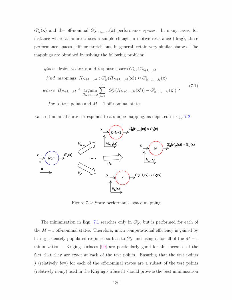
GsN(x) and the off-nominal Gs
N+1,...,M(x) performance spaces. In many cases, for
instance where a failure causes a simple change in motive resistance (drag), these
performance spaces shift or stretch but, in general, retain very similar shapes. The
mappings are obtained by solving the following problem:
given design vector x, and response spaces GsN , G
sN+1,...,M
find mappings HN+1,...,M : GsN(HN+1,...,M(x)) ≈ Gs
N+1,...,M(x)
where HN+1,...,M , argminHN+1,...,M
L∑
j=1
‖GsN(HN+1,...,M(xj))−Gs
N+1,...,M(xj)‖2
for L test points and M − 1 off-nominal states
(7.1)
Each off-nominal state corresponds to a unique mapping, as depicted in Fig. 7-2.
x
Nomx G��(x)
K=N+1x
K
MH���H� H�….
G��(H���(x)) ≈ G��(x)
G��(H�(x)) ≈ G��(x)x
x G��(H�(x)) ≈ G��(x)
M���(x)
H�(x)
H�(x)
Figure 7-2: State performance space mapping
The minimization in Eqn. 7.1 searches only in GsN , but is performed for each of
the M − 1 off-nominal states. Therefore, much computational efficiency is gained by
fitting a densely populated response surface to GsN and using it for all of the M − 1
minimizations. Kriging surfaces [99] are particularly good for this because of the
fact that they are exact at each of the test points. Ensuring that the test points
j (relatively few) for each of the off-nominal states are a subset of the test points
(relatively many) used in the Kriging surface fit should provide the best minimization
186

results.
The above approach was tested on the multistate Gaussian function described in
Appendix D in order to demonstrate that the process shows increased computational
efficiency for a relatively simple case with only two design variables. Four scenarios
were run, each withM=64 states and L=30 test points. These scenarios were intended
to determine:
1. Total number of function evaluations required to perform state performance
mapping in Eqn. 7.1 without response surface modeling.
2. Total number of function evaluations required to perform state performance
mapping in Eqn. 7.1 with response surface modeling of the nominal state.
3. Total number of function evaluations required to solve the optimization of
Eqn. 4.9 in Chapter 4, but for expected performance instead of availability.
This was performed without response surface modeling or performance map-
ping.
4. Total number of function evaluations required to do 3. above with response
surface modeling and performance mapping.
A Kriging surface was used for all cases with a response surface. Enough points
were used in the fitting of this surface that the minimization in Eqn. 7.1 was able
to find the exact mapping parameters (which were known), thus there was negligible
accuracy lost due to the surface approximation and the expected performance minima
(- maxima) from 3. and 4. were nearly identical. Results were promising, and are given
in Table 7.1.
There are two important observations to make from Table 7.1. First, the approach
can significantly improve computational efficiency. The comparison between 3. and
4. shows over a 60% reduction in total required function evaluations to obtain nearly
identical solutions for the optimization minima. Second, comparison between 1. and
2. shows that this improvement would be impossible without use of the response
surface.
187
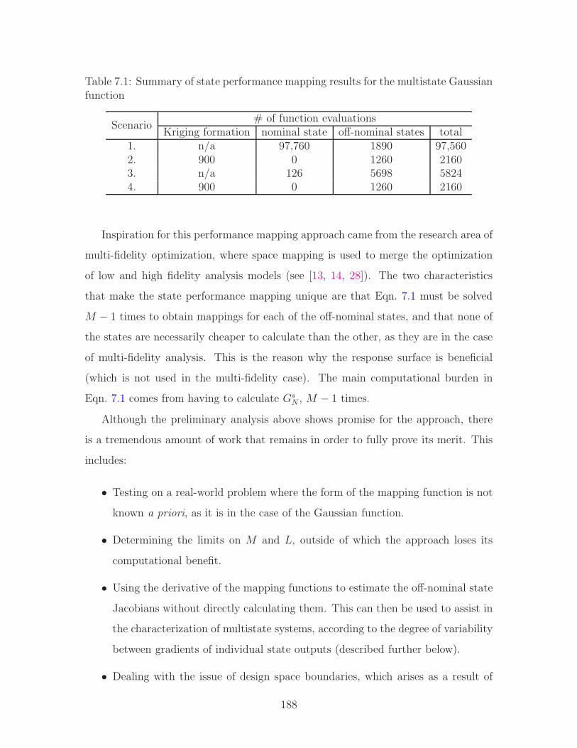
Table 7.1: Summary of state performance mapping results for the multistate Gaussianfunction
Scenario# of function evaluations
Kriging formation nominal state off-nominal states total1. n/a 97,760 1890 97,5602. 900 0 1260 21603. n/a 126 5698 58244. 900 0 1260 2160
Inspiration for this performance mapping approach came from the research area of
multi-fidelity optimization, where space mapping is used to merge the optimization
of low and high fidelity analysis models (see [13, 14, 28]). The two characteristics
that make the state performance mapping unique are that Eqn. 7.1 must be solved
M − 1 times to obtain mappings for each of the off-nominal states, and that none of
the states are necessarily cheaper to calculate than the other, as they are in the case
of multi-fidelity analysis. This is the reason why the response surface is beneficial
(which is not used in the multi-fidelity case). The main computational burden in
Eqn. 7.1 comes from having to calculate GsN , M − 1 times.
Although the preliminary analysis above shows promise for the approach, there
is a tremendous amount of work that remains in order to fully prove its merit. This
includes:
• Testing on a real-world problem where the form of the mapping function is not
known a priori, as it is in the case of the Gaussian function.
• Determining the limits on M and L, outside of which the approach loses its
computational benefit.
• Using the derivative of the mapping functions to estimate the off-nominal state
Jacobians without directly calculating them. This can then be used to assist in
the characterization of multistate systems, according to the degree of variability
between gradients of individual state outputs (described further below).
• Dealing with the issue of design space boundaries, which arises as a result of
188

some mappings requiring analysis beyond the original, nominal state design
space.
A second area recommended for future work involves further characterizing mul-
tistate systems according to the individual behaviors of their states. This will help
to better understand and predict the multistate performance trade-offs discussed in
Finding #3. Systems with a large degree of variability between gradients of indi-
vidual state outputs should exhibit larger trade-offs between nominal and expected
performance, and between availability and expected performance. The degree of this
opposition will be evident through the sensitivities in the multistate Jacobian, defined
here as,
∇Gs =
δGs1
δx1
δGs2
δx1· · · δGs
M
δx1
δGs1
δx2
δGs2
δx2· · · δGs
M
δx2
......
. . ....
δGs1
δxnx
δGs2
δxnx· · · δGs
M
δxnx
(7.2)
for nx design variables and K =M states.
As previously mentioned, it may be possible to efficiently determine this matrix
via performance mapping, or at least estimate it to a degree that allows predictions
to be made about the relative shapes of the state output spaces. Absent this, it is
still possible to directly calculate gradients at predetermined DOE points. In both
cases, the gradient information may then be used to pinpoint states that most conflict
with the nominal, or to gain a general understanding of the performance trade-offs
resulting from the multistate analysis.
As a final note on future work, there is one additional area where the methodology
described in this thesis might be used to push the envelope on performance and cost.
That is, namely, using multistate design to identify unnecessary design attributes
and eliminate them from the system in order to either save cost or improve overall
expected performance. Consider the design of a system composed of elements A, B,
and C. If the multistate design and analysis methodology can show that when B and
C fail, it is still possible to design with A such that the system achieves nominal or
189
near-nominal performance, it may be possible to go one step further and redesign the
system with A to absorb the functions of B and C, thus eliminating them.
In truth, instances such as this have already occurred in aerospace design, but
never from the probabilistic context of multistate analysis and design. The Northrop
B-2 bomber is a flying wing configuration that accomplishes lateral control through
split ailerons rather than a conventional tail. Although driven by the requirement
to have the smallest radar signature possible, the lack of a tail also significantly
reduces structural weight. Coaxial rotor helicopters achieve high lift through the use
of counter rotating propellers mounted on the same shaft structure. An added benefit
is that the torque generated from these main propellers can be used to accomplish the
same stability normally afforded by the tail rotor, thus eliminating the requirement
for an additional propeller on the tail.
The above examples have two things in common. First, they are enabled by high
powered computing. As this continues to increase, there are many performance gains
to be made from areas that have not traditionally been considered feasible options.
Secondly, they both require decisions to be made regarding the system’s geometric
design before the system is fielded. The probabilistic elements of multistate analysis
and design should prove very effective in predicting what these decisions should be.
190

Appendix A
6-DoF Multistate Aircraft Model
The twin-engine aircraft model used in the analysis of Chapter 3 is the product of a
larger multistate aircraft performance tool that resulted from this research. Although
flight simulation is the ultimate performance output of this higher fidelity conceptual
design routine, pseudo-instantaneous performance analysis may also be accomplished
by trimming for desired flight conditions across a very short time span. This technique
was effectively used in determination of the reachability criterion described at the end
of Chapter 3, using an optimization similar to that in Eqn. 3.6 to trim.
When using as a design tool for the conceptual or early-primary design stage,
it is not possible to know exact mass properties of every design variation, and it
is inherently impossible to flight-test validate each of the design points. Thus, the
accuracy of the performance analysis will be partially limited by these conceptual
level estimates, even though the accuracy of the simulation output is likely higher
than typical conceptual level design.1
Nonetheless, there are two other advantages that make this multistate performance
tool desirable. The first is that it automates the translation of typical conceptual
level design variables such as wingspan, aspect ratio, tail geometry, etc., into the full
set of aerodynamic properties output by AVL. These are then defined as internal
properties in the flight simulation, such that they can be updated at every time step,
1For the case of the Super King Air, these limitations were partially offset by comparing thebaseline design to several flight test data points and making sure that the models agreed.
191

if desired. The second is that failures can be input into the analysis during runtime,
and dynamic effects of the resulting performance may be approximated. Ultimately,
the author intends to use this as part of a conceptual aircraft design curriculum,
where students design and size their aircraft based on top-level mission requirements,
and are then able to personally fly what they have designed in the full 6-DoF flight
simulator within a matter of minutes.
A.1 Mass and Inertias
Aircraft mass properties, including exact values for individual moments of inertia,
mass, and centers of gravity for each of the aircraft components, can be entered
directly into the performance simulation module. When executed as part of the
design loop, however, a separate mass properties module calculates the mass of each
of these values using empirically based equations from Brandt et al. [25] and Roskam
[92]. These are mass estimations commonly used in conceptual level design, and take,
for instance, the form of Eqn. A.1 for wing mass [92].
mwing = 0.033Sn0.2maxA1.8(1 + λ)0.5
(t/c)0.7cos ΛLE
(A.1)
The standard practice for using such estimates is to verify that output is valid for
the type of aircraft being designed (through comparison to already existing aircraft),
and adjust the appropriate factors accordingly. In the case of the Super King Air,
the component estimates were verified and adjusted (i.e., the leading coefficient of
Eqn. A.1) against the exact data given in [37] for the Beech Model 200, as well as
against weight and balance sheets for operational USAF C-12’s.
The research developed code calculates inertias for each of these components by
volumetrically discretizing them into smaller divisions, computing the divisional cen-
ters of gravity, and summing the discretized inertias, according to formulae such as
Eqn. A.2.
Ixx,comp =∑
mi(y2i,c.g. + z2i,c.g.) (A.2)
192
where
mi = Vi ∗ fiD (A.3)
and fi is a weighting factor on component density, D, such that it satisfies,
D =
∑
fiD
# divisions=mcomp∑
Vi
(A.4)
This provides Ixx, Iyy, Izz, and Ixz for the wing, tail, fuselage, etc. The parallel axis
theorem is then used to calculate total inertias for the aircraft. Comparison to the
actual inertias in [37] for the Beech 200 showed that this method was very accurate,
given proper component weights. Where discrepancies existed, the weighting fac-
tor, fi, was easily adjusted to control component density distributions, until inertias
matched. In general, the products of inertia, Ixy and Iyz, are neglected when the
aircraft has symmetry of mass and geometry about these axes (as most do).
A.2 Aerodynamic Forces and Moments
All lift-affected aerodynamics are computed through Athena Vortex Lattice (AVL),
which employs an extended vortex lattice model for lifting surfaces and a slender
body model for fuselages and nacelles. Documentation is extensive and is found in
[8]. As AVL input files are cumbersome and require significant work to correctly
construct, a pre-processing routine was developed that takes general aircraft design
variables and geometry as input, and gives the appropriate AVL input file as output.
The AVL output is then post-processed into a format that can be passed directly to
the modified JSBSim flight simulator. This enables AVL to be directly integrated
into the design loop for any desired flight condition.
There are two methods used to complete the drag polar with the addition of
non-lift-induced drag (a.k.a. parasite drag, CDo). The first is to simply supply AVL
with a known value of CDofrom flight test for the appropriate flight conditions and
configuration. This will be accurate for the baseline aircraft. A second method,
which proves very accurate for subsonic conditions [25], is to use an estimate based
193
on drag data for similar aircraft under the concept of an equivalent skin-friction drag
coefficient, Cfe, defined in:
CDo= Cfe
Swet
S(A.5)
There is a large database of values for Cfe for several classes of aircraft in [86, 91].
The advantage of the second method is that both S and Swet are functions of aircraft
geometry, thus CDocan be calculated for differing design points. In the twin-engine
aircraft case, the above two methods were combined, using the flight test value for
the baseline aircraft to provide Cfe, such that Eqn. A.5 could then be used for the
perturbed design points.
In addition to overall aircraft lift and drag characteristics, control derivatives for
the aileron, rudder, and elevator are computed in AVL and used as input to the flight
simulation routine. The process is to compute each of these derivatives for a range
of angles-of-attack (in the Super King Air case, this was -4◦ to 14◦) at the target
maneuver flight conditions for each design geometry. This entire range is then read
into the flight simulation code as a look-up table, and accessed depending on control
inputs at each time step. If maneuver flight conditions vary enough that the control
derivatives are no longer valid, the look-up table format is extensible to multiple
dimensions, where data points between pre-computed AVL flight conditions can be
rapidly interpolated. This has little to no effect on (simulation) run-time as all of the
simulation takes place within a C++ executable and is extremely fast. This property of
the core JSBSim code makes it extremely powerful as a tool for performance analysis.
A.3 Performance Simulation Through JSBSim
JSBSim [18] is an open-sourced, GNU licensed collection of 6-DoF flight simulation
libraries written in C++. It has been under development by dozens of engineers for
over ten years. Input to JSBSim is typically done through a front-end .xml input
file, where the aircraft’s characteristic parameters are read in once at the onset of the
simulation and then control inputs are treated as dynamic properties updated several
times per second during run-time. Mills [76] began work on the basic implementation
194

of a MATLAB S-Function over three years ago and work for this thesis picked up from
his work, making modifications to the flight simulation engine itself. The resulting
updates focused on two areas:
• Bypassing the standard .xml input file so that aircraft characteristics are read
directly from geometry, mass, and aerodynamics modules
• Rewriting and recompiling the source code such that all aircraft design variables
are defined as time dependent inputs within the simulation executable
This enables the effects of aircraft design variables to be treated as dynamic properties
in the same way as control inputs, such that they can be varied as a functions of
time during the execution of the flight model in Simulink. It makes possible the
rapid evaluation of a wide range of aircraft performance parameters for a nearly
limitless number of aircraft configurations, including simulation of failure states, e.g.
loss of actuators and engine failures. Additionally, it makes possible the in-flight
physical reconfiguration of the aircraft, whether that be due to a failure (such as loss
of vertical stabilizer) or variation of wing geometry (i.e. sweep, aspect ratio). If a
more traditional analysis is desired, the variables are simply held fixed throughout
the simulation.
There are over 70 C++ classes that make up JSBSim, as shown in the hierarchy
of Fig. A-1. These classes fall into several categories, including math, input/output,
initialization, model, and basic. In order to facilitate the modeling of arbitrary vehicle
configurations, the framework is based around flexible object oriented modeling for the
propulsion system, aerodynamic characteristics, control system, and ground reaction
mechanisms. The JSBSim input set, as defined within the multistate design loop,
is given in Fig. A-2, where all of the aerodynamic coefficients come from AVL. The
output set is found in Fig. A-3. This is actually only a subset of possible outputs, but
encompasses the typical 6-DoF output vector [U, V,W, P,Q,R, φ, θ, ψ, posN , posE, h].
In practice, both input and output are row oriented matrices with the number of
columns equal to the number of time-steps within the simulation.
195

Figure A-1: JSBSim class hierarchy [19]
196

�� � � � �� � � �� � � �� � �� � � � � �� �� � � � �� � � �� � � �� � �� � � � � �� ¡ ¢£¤ ¡ ¡ ¥¦ § ¨© ª § § «¬ ª® ¯ § ¯ ª° ±² ³ ´ µ ¶·¸ ¹º » ¼½ « ¯ ¾ §¿ ª¬ ¾ ¾ ¯¿ ¯¬ ° § ¾ ª© À© Á ª « Á© Á § § Á©  ¬ § ¾ « ¯  ¨ § Á « § ¯ §Ã À¬ ° Ä Á Å Æ ¥¦ £¤ Ç « ¬ ¾ § Á ¯ «¬ © ª ° ª® ¯ § ¯ ª ° ±² ³ ´ µ ¶·¸ ¹º » È ½ « ¯ ¾ §¿ ª¬ ¾ ¾ ¯¿ ¯¬ ° § ¾ ª© À© Á ª « Á© Á § § Á©  ¬ § ¾ « ¯  ¨ § Á « § ¯ §Ã À¬ ° Ä Á ¦ ¥ ¦É Å ¡ ¤ £ ¬ «¬ Ê Á § ª© ª ® ¯ § ¯ ª ° ±² ³ ´ µ ¶·¸ ¹º » Ë ½ « ¯ ¾ §¿ ª¬ ¾ ¾ ¯¿ ¯¬ ° § ¾ ª© À© Á ª « Á© Á § § Á©  ¬ § ¾ « ¯  ¨ § Á « § ¯ §Ã À¬ ° Ä Á £Ì Í Í¦ £ © à À À¬ © ª® ¯ § ¯ ª ° ±² ³ ´ µ ¶ ·¸ ¹º » ÎÏ ½ « ¯ ¾ §¿ ª¬ ¾ ¾ ¯¿ ¯¬ ° § ¾ ª© À© Á ª « Á© Á § § Á©  ¬ § ¾ « ¯  ¨ § Á « § ¯ §Ã À¬ ° Ä Á ¦ ÇÐ Æ Ç ¦ ¬ °  ¯ ° ¬ Ñ ¯Ò § à © ¬ ±² ³ ´ µ ¶ ·¸ ¹º » ÎÓ ½ « ¯ ¾ §¿ ª¬ ¾ ¾ ¯¿ ¯¬ ° § ¾ ª© À© Á ª « Á© Á § § Á©  ¬ § ¾ « ¯  ¨ § Á « § ¯ §Ã À¬ ° Ä Á Ô Å Ð Ç¦ ¡ ¤ Ñ Á ° ¬ § ª ª® ¯ § ¯ ª ° ±² ³ ´ µ ¶ ·¸ ¹º » Î ¼½ « ¯ ¾ §¿ ª¬ ¾ ¾ ¯¿ ¯¬ ° § ¾ ª© À© Á ª « Á© Á § § Á©  ¬ § ¾ « ¯  ¨ § Á « § ¯ §Ã À¬ ° Ä Á Õ ¥ÅÖ ¾ « Á ª ® ¯ § ¯ ª ° ±² ³ ´ µ ¶× ¸ ¹ º »Ø ¼½ À © Á ¿ ª¬ ¾ ¾ ¯¿ ¯¬ ° § ¾ ª© À© Á ª « Á© Á § § Á©  ¬ § ¾ « ¯  ¨ § Á « § ¯ §Ã À¬ ° Ä Á Ð ¦ Å £  ¬ Á© ª® ¯ § ¯ ª ° ±² ³ ´ µ ¶× ¸ ¹ º »Ø Ó ½ À © Á ¿ ª¬ ¾ ¾ ¯¿ ¯¬ ° § ¾ ª© À© Á ª « Á© Á § § Á©  ¬ § ¾ « ¯  ¨ § Á « § ¯ §Ã À¬ ° Ä Á¶ ·¸ ÙÕ ¥ÅÖ ¿ ¨ Á °  ¬ ¯ ° « ¯ ¾ §¿ ª¬ ¾ ¾ ¯¿ ¯¬ ° § À à ¬ § ª ¾ « Á À¬ ¾ «¬ ¿ § ¯ ª ° ° Ä Á ¶× ¸ ¹º »Ï ½ À © Á ¿ ª¬ ¾ ¾ ¯¿ ¯¬ ° § ¾ ª© À© Á ª « Á© Á § § Á©  ¬ § ¾ « ¯  ¨ § Á « § ¯ §Ã À¬ ° Ä Á¶·¸ Ù¦ ¥¦ É Å ¡ ¤ £ ¿ ¨ Á °  ¬ ¯ ° « ¯ ¾ §¿ ª¬ ¾ ¾ ¯¿ ¯¬ ° § À à ¬ § ª ¬ «¬ Ê Á § ª© À¬ ¾ «¬ ¿ § ¯ ª ° ° Ä Á ¶× ¸ ¹º »Ó ½ À © Á ¿ ª¬ ¾ ¾ ¯¿ ¯¬ ° § ¾ ª© À© Á ª « Á© Á § § Á©  ¬ § ¾ « ¯  ¨ § Á « § ¯ §Ã À¬ ° Ä Á¶× ¸ ÙÕ ¥ÅÖ ¿ ¨ Á °  ¬ ¯ ° À© Á ¿ ª¬ ¾ ¾ ¯¿ ¯¬ ° § À à ¬ § ª ¾ « Á À¬ ¾ «¬ ¿ § ¯ ª° ° Ä Á ¶× ¸ ¹º » ¼ ½ À © Á ¿ ª¬ ¾ ¾ ¯¿ ¯¬ ° § ¾ ª© À© Á ª « Á© Á § § Á©  ¬ § ¾ « ¯  ¨ § Á « § ¯ §Ã À¬ ° Ä Á¶× ¸ Ù¦ ¥¦ É Å ¡ ¤ £ ¿ ¨ Á °  ¬ ¯ ° À© Á ¿ ª¬ ¾ ¾ ¯¿ ¯¬ ° § À à ¬ § ª ¬ «¬ Ê Á § ª© À¬ ¾ «¬ ¿ § ¯ ª ° ° Ä Á ¶× ¸ ¹º » È ½ À © Á ¿ ª¬ ¾ ¾ ¯¿ ¯¬ ° § ¾ ª© À© Á ª « Á© Á § § Á©  ¬ § ¾ « ¯  ¨ § Á « § ¯ §Ã À¬ ° Ä Á¶ ¥Ú ¿ ¨ Á °  ¬ ¯ ° © ª « « ¯ ° ÂÛ Ñ ª Ѭ ° § ¿ ª¬ ¾ ¾ ¯¿ ¯¬ ° § Ü ¯ § ¨ ® ¯ À¬ ® « ¯ Á °  «¬ ° Ä Á ¶× ¸ ¹º » Ë ½ À © Á ¿ ª¬ ¾ ¾ ¯¿ ¯¬ ° § ¾ ª© À© Á ª « Á© Á § § Á©  ¬ § ¾ « ¯  ¨ § Á « § ¯ §Ã À¬ ° Ä Á¶ ¥Ö ¿ ¨ Á °  ¬ ¯ ° © ª « « ¯ ° ÂÛ Ñ ª Ѭ ° § ¿ ª¬ ¾ ¾ ¯¿ ¯¬ ° § Ü ¯ § ¨ © ª « « © Á §¬ ° Ä Á ¶× ¸ ¹º » ÎÏ ½ À © Á ¿ ª¬ ¾ ¾ ¯¿ ¯¬ ° § ¾ ª© À© Á ª « Á© Á § § Á©  ¬ § ¾ « ¯  ¨ § Á « § ¯ §Ã À¬ ° Ä Á¶ ¥£ ¿ ¨ Á °  ¬ ¯ ° © ª « « ¯ ° ÂÛ Ñ ª Ѭ ° § ¿ ª¬ ¾ ¾ ¯¿ ¯¬ ° § Ü ¯ § ¨Ý Á Ü © Á §¬ ° Ä Á ¶× ¸ ¹º » ÎÓ ½ À © Á ¿ ª¬ ¾ ¾ ¯¿ ¯¬ ° § ¾ ª© À© Á ª « Á© Á § § Á©  ¬ § ¾ « ¯  ¨ § Á « § ¯ §Ã À¬ ° Ä Á¶ ¥¸ ÙÅ Æ ¥¦ £ ¤ Ç ¿ ¨ Á °  ¬ ¯ ° © ª « « ¯ ° ÂÛ Ñ ª Ѭ ° § ¿ ª¬ ¾ ¾ ¯¿ ¯¬ ° § Ü ¯ § ¨ Á ¯ « ¬ © ª ° À¬ ¾ «¬ ¿ § ¯ ª ° ° Ä Á ¶× ¸ ¹º » Î ¼½ À © Á ¿ ª¬ ¾ ¾ ¯¿ ¯¬ ° § ¾ ª© À© Á ª « Á© Á § § Á©  ¬ § ¾ « ¯  ¨ § Á « § ¯ §Ã À¬ ° Ä Á¶ ¥¸ Ù£Ì Í Í ¦ £ ¿ ¨ Á °  ¬ ¯ ° © ª « « ¯ ° ÂÛ Ñ ª Ѭ ° § ¿ ª¬ ¾ ¾ ¯¿ ¯¬ ° § Ü ¯ § ¨ © à À À¬ © À¬ ¾ «¬ ¿ § ¯ ª ° ° Ä Á Þwing
Ü ¯ °  Á© ¬ Á ¾ §2¶Ô º ¿ ¨ Á °  ¬ ¯ ° ¯ §¿ ¨ ¯ ° Â Û Ñ ª Ѭ ° §¿ ª¬ ¾ ¾ ¯¿ ¯¬ ° § Ü ¯ § ¨ Á °  « ¬ Û ª ¾Û Á § § Á¿ ß ° Ä Á àwing
Ü ¯ °  ® Á ° ¾ §¶Ô ¸ Ù¦ ¥ ¦É Å ¡ ¤ £ ¿ ¨ Á °  ¬ ¯ ° ¯ §¿ ¨ ¯ ° Â Û Ñ ª Ѭ ° §¿ ª¬ ¾ ¾ ¯¿ ¯¬ ° § Ü ¯ § ¨ ¬ « ¬ Ê Á § ª© À¬ ¾ «¬ ¿ § ¯ ª ° ° Ä Á ¿wing
Ü ¯ °  ¿ ¨ ª© À ¾ §¶Ô á ¿ ¨ Á °  ¬ ¯ ° ¯ §¿ ¨ ¯ ° Â Û Ñ ª Ѭ ° §¿ ª¬ ¾ ¾ ¯¿ ¯¬ ° § Ü ¯ § ¨ ¯ §¿ ¨ © Á §¬ ° Ä Á Þht
¨ ª© ¯â ª ° § Á « § Á ¯ « Á© ¬ Á ¾ §2¶Ô ¸ ÙÕ ¥ÅÖ ¿ ¨ Á °  ¬ ¯ ° ¯ §¿ ¨ ¯ ° Â Û Ñ ª Ѭ ° §¿ ª¬ ¾ ¾ ¯¿ ¯¬ ° § Ü ¯ § ¨ ¾ « Á À¬ ¾ «¬ ¿ § ¯ ª ° ° Ä Á «ht
¨ ª© ¯â ª ° § Á « § Á ¯ « Á© Ñ ¾ §¶ ÇÚ ¿ ¨ Á °  ¬ ¯ ° Ý Á Ü ¯ ° Â Û Ñ ª Ѭ ° §¿ ª¬ ¾ ¾ ¯¿ ¯¬ ° § Ü ¯ § ¨ ® ¯ À¬ ® « ¯ Á °  «¬ ° Ä Á Þvt
ʬ © § ¯¿ Á « § Á ¯ « Á© ¬ Á ¾ §2¶ Ç£ ¿ ¨ Á °  ¬ ¯ ° Ý Á Ü ¯ ° Â Û Ñ ª Ѭ ° §¿ ª¬ ¾ ¾ ¯¿ ¯¬ ° § Ü ¯ § ¨Ý Á Ü © Á §¬ ° Ä Á «vt
ʬ © § ¯¿ Á « § Á ¯ « Á© Ñ ¾ §¶ Ǹ Ù£Ì Í Í ¦ £ ¿ ¨ Á °  ¬ ¯ ° Ý Á Ü ¯ ° Â Û Ñ ª Ѭ ° §¿ ª¬ ¾ ¾ ¯¿ ¯¬ ° § Ü ¯ § ¨ © à À À¬ © À¬ ¾ «¬ ¿ § ¯ ª ° ° Ä Á Òa.c.
Á ¯ © ¿ © Á ¾ § Á¬ © ª ÀÝ ° Á Ñ ¯¿ ¿ ¬ ° §¬ © ³ Ò Û ¿ ª ª© À ¯ ° Á §¬ ¯ °¶
n,
ã
aileron
¿ ¨ Á °  ¬ ¯ ° Ý Á Ü ¯ ° Â Û Ñ ª Ѭ ° §¿ ª¬ ¾ ¾ ¯¿ ¯¬ ° § Ü ¯ § ¨ Á ¯ «¬ © ª ° À¬ ¾ «¬ ¿ § ¯ ª ° ° Ä Á Ýa.c.
Á ¯ © ¿ © Á ¾ § Á¬ © ª ÀÝ ° Á Ñ ¯¿ ¿ ¬ ° §¬ © ³Ý Û ¿ ª ª© À ¯ ° Á §¬ ¯ °¶
Y
ä ¿ ¨ Á °  ¬ ¯ ° ® ¯ À¬ Û ¾ ª© ¿ ¬ ¿ ª¬ ¾ ¾ ¯¿ ¯¬ ° § Ü ¯ § ¨ ® ¯ À¬ ® « ¯ Á °  «¬ ° Ä Á âa.c.
Á ¯ © ¿ © Á ¾ § Á¬ © ª ÀÝ ° Á Ñ ¯¿ ¿ ¬ ° §¬ © ³ âÛ ¿ ª ª© À ¯ ° Á §¬ ¯ °¶
Yp
¿ ¨ Á °  ¬ ¯ ° ® ¯ À¬ Û ¾ ª© ¿ ¬ ¿ ª¬ ¾ ¾ ¯¿ ¯¬ ° § Ü ¯ § ¨ © ª « « © Á §¬ ° Ä Á Ò åæ Ð æ .
Á ¯ © ¿ © Á ¾ § ¿ ¬ ° §¬ ©Û ª ¾Û  © Á Ê ¯ §Ý ³ Ò Û ¿ ª ª© À ¯ ° Á §¬ ¯ °¶
Y,
ã
rudder
¿ ¨ Á °  ¬ ¯ ° ® ¯ À¬ Û ¾ ª© ¿ ¬ ¿ ª¬ ¾ ¾ ¯¿ ¯¬ ° § Ü ¯ § ¨ © à À À¬ © À¬ ¾ «¬ ¿ § ¯ ª ° ° Ä Á Ý åæ Ð æ .
Á ¯ © ¿ © Á ¾ § ¿ ¬ ° §¬ ©Û ª ¾Û  © Á Ê ¯ §Ý ³Ý Û ¿ ª ª© À ¯ ° Á §¬ ¯ °¶
Y,
ã
aileron
¿ ¨ Á °  ¬ ¯ ° ® ¯ À¬ Û ¾ ª© ¿ ¬ ¿ ª¬ ¾ ¾ ¯¿ ¯¬ ° § Ü ¯ § ¨ Á ¯ « ¬ © ª ° À¬ ¾ «¬ ¿ § ¯ ª ° ° Ä Á Ò åæ Ð æ .
Á ¯ © ¿ © Á ¾ § ¿ ¬ ° §¬ ©Û ª ¾Û  © Á Ê ¯ §Ý ³ âÛ ¿ ª ª© À ¯ ° Á §¬ ¯ °¶·¸ ¹º »Ø ¼ ½ « ¯ ¾ §¿ ª¬ ¾ ¾ ¯¿ ¯¬ ° § ¾ ª© À© Á ª « Á© Á § § Á©  ¬ § ¾ « ¯  ¨ § Á « § ¯ § à À¬ ° Ä Á çxx
Ñ ª Ѭ ° § ª ¾ ¯ ° ¬ © § ¯ Á Á à ª à § Ò Û ÁÒ ¯ ® ® « è ¾ §2¶·¸ ¹º »Ø Ó ½ « ¯ ¾ §¿ ª¬ ¾ ¾ ¯¿ ¯¬ ° § ¾ ª© À© Á ª « Á© Á § § Á©  ¬ § ¾ « ¯  ¨ § Á « § ¯ § à À¬ ° Ä Á ç
yy
Ñ ª Ѭ ° § ª ¾ ¯ ° ¬ © § ¯ Á Á à ª à §Ý Û ÁÒ ¯ ® ® « è ¾ §2¶·¸ ¹ º »Ï ½ « ¯ ¾ §¿ ª¬ ¾ ¾ ¯¿ ¯¬ ° § ¾ ª© À© Á ª « Á© Á § § Á©  ¬ § ¾ « ¯  ¨ § Á « § ¯ § à À¬ ° Ä Á ç
zz
Ñ ª Ѭ ° § ª ¾ ¯ ° ¬ © § ¯ Á Á à ª à § âÛ ÁÒ ¯ ® ® « è ¾ §2¶·¸ ¹ º »Ó ½ « ¯ ¾ §¿ ª¬ ¾ ¾ ¯¿ ¯¬ ° § ¾ ª© À© Á ª « Á© Á § § Á©  ¬ § ¾ « ¯  ¨ § Á « § ¯ § à À¬ ° Ä Á éê Á ¯ © ¿ © Á ¾ §  © ª® ® ܬ ¯  ¨ § « à
Figu
reA-2:
Perform
ance
simulation
inputset
197

ëìíîìïðñ òñóôíîõöî÷ø ùøîöóú ûü ýþÿ��� �ýþ�� ������ ��� ûü ýþÿ��� �ýþ�� ������ ��� ûü ýþÿ��� �ýþ�� ����� ��� �þýý ���ü ����� ���ÿ� ���ü ����� ��� ���ü �����þ�� �üþ������ÿ ýþ������ü �ü���� �üþ������ÿ ý������ü �ü����� �üþ�ü��ÿ �ý�����ü �� �þýý ���ýü ���� ���ÿ� ���ýü ���� ��� ���ýü ���� �ý�����ü �� ���ýü�þ�����ÿ� ��� ���ýü�þ����ü�ý�� ���� ûü���ÿ�ý �ÿÿü ýü����þ� ��!�dot
����ý�� �ÿÿü ýü����þ� �"þ�� ������ ����! dot
����ý�� �ÿÿü ýü����þ� �"þ�� ����� ����!# #�ÿ� ��$"ü� ���C
ÿ�ý�"���ü� �����üü� ��þ���E
ü%��û�ýü�� �����üüü� ��þ���eng1
ü����ü �þ�ü� &��eng2
ü����ü �þ�ü� &�'( ü����ü ��$ �üû$��') ü����ü ��$ �üû$��** �ü ý ýþ� ���ü ý"$��Figure A-3: Performance simulation output subset
198
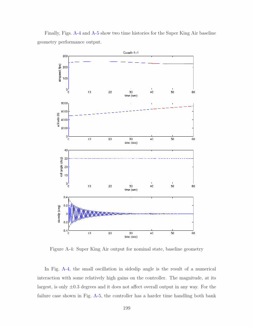
Finally, Figs. A-4 and A-5 show two time histories for the Super King Air baseline
geometry performance output.
Figure A-4: Super King Air output for nominal state, baseline geometry
In Fig. A-4, the small oscillation in sideslip angle is the result of a numerical
interaction with some relatively high gains on the controller. The magnitude, at its
largest, is only ±0.3 degrees and it does not affect overall output in any way. For the
failure case shown in Fig. A-5, the controller has a harder time handling both bank
199

and sideslip with only the rudder, but eventually manages to dampen out the longer
period oscillations.
Figure A-5: Super King Air output for baseline geometry, left engine and aileronsfailed
200
A.4 Controls
JSBSim also incorporates the ability to build up entire flight control systems using
series of components to model filters, switches, summers, gains, sensors, etc. This was
how the PID controller in Fig. 3-7, of Chapter 3, was constructed, where the gains
were defined as design variables within the design loop. Although the multistate
performance model is executed as part of an S-function, and thus has all of the
traditional Simulink controllers at its disposal, allowing the flight simulator to perform
these tasks was several orders of magnitude faster since all sensing and feedback was
performed internally within the C++ executable. In either case, however, it was
verified that the results were the same.
A.5 Propulsion
The propulsion module takes the form of engine and thruster decks within JSBSim.
It supports piston, turbine, rocket, and electric engine force, moment, and fuel con-
sumption calculations. For the vehicle’s desired thrust mechanism, the engine model
(e.g. turboprop) is coupled with the thruster definition (e.g. propeller) to model the
aircraft’s overall thrust characteristics. The basic power output of the engine as a
function of altitude and airspeed comes from the engine deck in the form of a look-up
table. Effects of the propeller are integrated into this model by using specification ta-
bles for thrust and power coefficient as a function of advance ratio and blade-angle (in
the case of variable pitch propellers). Additional effects that can be modeled include
gyroscopic effects due a spinning drive shaft and propeller, and P-factor. P-factor is
a phenomenon that occurs in a climbing aircraft due to the fact that the downward
arcing propeller blade has a higher angle of attack relative to wind velocity than the
upward arcing blade, and thus higher thrust. In an aircraft with clockwise spinning
propellers, this results and yawing moment to the left. P-factor is approximated in
JSBSim by shifting the point of application of the thrust vector over the propeller
disk as a function of α (angle-of-attack).
201

202
Appendix B
Twin-engine Aircraft Reachability
Analysis
********************************
In Appendix B only, the term state, unless capitalized and
followed by a number, refers to state in the context of a con-
tinuous state-space in controls theory, rather than the discrete
performance-based states used throughout the rest of the thesis.
Additionally, x refers to the state vector rather than the static
design vector, in order to conform with traditional controls the-
ory nomenclature.
********************************
The purpose of the reachability analysis is ensure that the results of the worst
performing states were not merely due to an inappropriate selection of gains for the
specified control system, but that they truly were unachievable, given the system
configuration. One means of doing this was a careful formulation of the gain opti-
mization given in Eqn. 3.6, examination of the resulting post-optimality criterion,
and comparison of results from multiple starting points within the design space, all of
which indicated the best possible solution had been obtained. As a second means of
203
verification, a comparison of system reachability was made between satisfactory and
non-satisfactory geometries, a full discussion of which is provided below.
The state-space system described by
x = Ax +Bu
y = Cx+Du(B.1)
in which x(t) ∈ Rn is the state vector, u(t) ∈ R
m is the input vector, and y(t) ∈ Rp is
the output vector, is termed reachable if a control input can be selected to drive the
system from any initial state to any final state in time t. This solves the problem of
determining whether it is possible, given the current system configuration, of reaching
the desired final state. The are many techniques available for solving the reachability
problem for discrete time, one of which is the formation and analysis of the reachability
matrix, which is defined as
Z = [B|AB|A2B|...|An−1B] ∈ Rnxnm (B.2)
If and only if the matrix Z has full rank n is the system reachable. This charac-
teristic arises from the nature of the system zeros, which may be divided into three
categories: input-decoupling zeros, output-decoupling zeros, and transmission zeros.
Only the input-decoupling zeros will be discussed here as they are most relevant to
the reachability problem, but the reader is directed to [7] and [89] for a full treatment
of the topic.
The above mentioned zeros for a multiple-input multiple-output (MIMO) system
can be derived from the Rosenbrock system matrix, given in the Laplace domain as
F (s) =
sI −A B
C D
(B.3)
204
The input-decoupling zeros are the values of s where the upper block matrix (de-
scribing the input coupling) of Eqn. B.3, given below as Eqn. B.4,
Fupper(s) = [sI −A|B] ∈ Rnx(n+m) (B.4)
has rank less than n. This occurs when multiple paths exist to the same system output
or alternate physical mechanisms result in competing output components [101]. The
existence of input-decoupling zeros means that control effectiveness is unachievable
with the given set of inputs. Furthermore, reachability is equivalent to the absence of
input-decoupling zeros.
Eqns. B.2 and B.4 provide a convenient means for verifying the performance of
the worst performing states as reported in Section 3.3. As an example, consider the
results shown in State 4 of Fig. 3-9. Here, Eqns. B.2 and B.4 were used to determine
the reachability of the baseline geometry system as compared to the low tail height
geometry system, where the baseline geometry performance fell well within the safe
region, while the low tail height geometry was the leftmost point outside of the it.
The initial step in this process was to construct the state-matrix A, the control-
matrix B, and the output-matrix C (the feed-forward matrix D was null). This
was accomplished using an interior-point optimization algorithm acting on the state
derivatives to trim the aircraft model as close as possible to the desired flight condi-
tions for both geometries. The model was then linearized about these points using
an algorithm adapted from Stevens and Lewis [101], in order to obtain two dis-
tinct, geometry-specific sets of (A, B, C). Although only A and B are needed for
the evaluation of Eqn. B.2, C was used to find the system zeros from Eqn. B.3
for the rank evaluation of Eqn. B.4. For State 4, the state vector consisted of
[U, V,W, P,Q,R, φ, θ, ψ, posN , posE, h] (following notation from the standard equa-
tions of motion), while the input vector was [δelevator , δrudder] with output of [P,R, φ, ψ],
recalling that for State 4 the ailerons and left engine were failed.
Results showed a distinct difference in the degree of reachability for the two ge-
ometries. The rank of Z from Eqn. B.2 for the baseline geometry was 12 (full rank
205

since n = 12), indicating a reachable system. For the low tail geometry, the rank
dropped to 11 for the same tolerances, indicating an unreachable system and imply-
ing the existence of one or more input-decoupling zeros. Further examination of the
system zeros and subsequent evaluation of Fu(s) from Eqn. B.4 showed the presence
of one input-decoupling zero near the origin for the low tail geometry and confirmed
the absence of input-decoupling zeros for the baseline geometry system. Thus, the
analysis confirmed that, in cases where the simulation resulted in unsatisfactory state
performance, this was truly due to the physical configuration of the system, and not
to the inappropriate selection of controller gains.
206

Appendix C
Sorting Algorithm for Multilayer
Markov Analysis
The following algorithm is used to sort and bin probabilities resulting from the Ve-
hicle Markov Model (VMM), based on the sortie performance thresholds, such that
they may be aggregated into Sortie Equivalent Markov Model (SEMM) probabilities
(Section 4.2.1, Chapter 4). The algorithm specifically applies to a model with four
performance categories, nominal(N), degraded(D), abort(A), and loss(L), but could
be extended to additional categories if necessary. This extension would simply re-
quire additional tiers of performance categorization, being sure to include the code
within the while loop for downstream categories that are spanned by multiple levels
of failure.
Inputs: Probability set from Vehicle Markov Model, PVMM; Performance set fromVehicle Markov Model, GVMM; Index set of previous Vehicle Markov Model states,SVMMprev , the elements of which comprise the states from which each state arrives;
and Sortie Equivalent Markov Model performance thresholds W = [Wmin,N Wmin,D
Wmin,A]. Each of the above are size MVMM , except for W
Outputs: Probability set for Sortie Equivalent Markov Model, PSEMM
207

Initialize variablesdeclare IN, ID, IA, IL, INA, IDA, INL, IDL, INAL, IDAL, c, m, n, q, r
Check that nominal state achieves nominal performanceif GVMM(1) < Wmin,N
display “error, nominal performance not met”end if
PERFORM TOP-TIER PERFORMANCE CATEGORIZATIONm = n = q = r = 1for i = i...MV MM
if GVMM(i) ≥Wmin,N
IN(m) = im = m+ 1
else if GVMM(i) ≥Wmin,D
ID(n) = in = n+ 1
else if GVMM(i) ≥Wmin,A
IA(q) = iq = q + 1
elseIL(r) = ir = r + 1
end ifend for
PERFORM 2ND-TIER PERFORMANCE CATEGORIZATION:Determine which abort states come from nominal or degraded statesm = n = 1for i = 1...number of elements in IA
if SVMMprev (IA(i)) ∈ ININA(m) = IA(i)m = m+ 1
else if SVMMprev (IA(i)) ∈ ID
IDA(n) = IA(i)n = n+ 1
end ifend for
Check for abort states that come from other abort states and add to correct pathc = 1while number of elements in c > 0, do
c = IA\{INA IDA} (the excluded set)for i = 1...number of elements in c
if SVMMprev (c(i)) ∈ INA
208
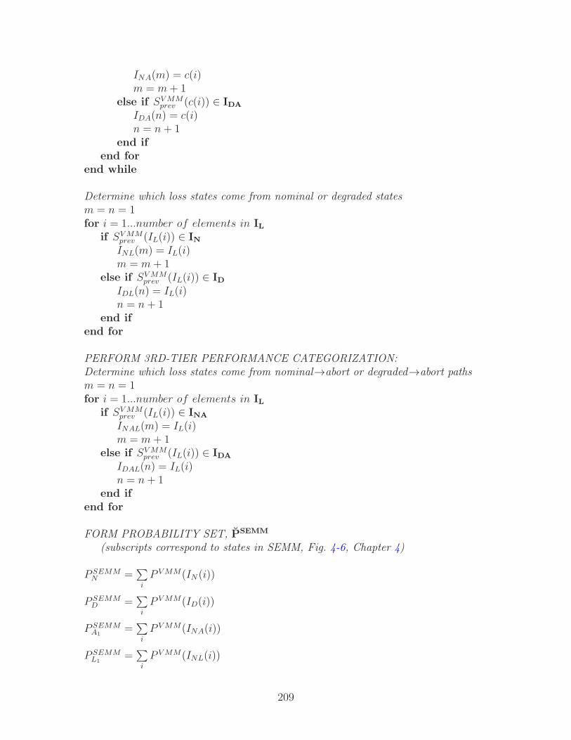
INA(m) = c(i)m = m+ 1
else if SVMMprev (c(i)) ∈ IDA
IDA(n) = c(i)n = n + 1
end ifend for
end while
Determine which loss states come from nominal or degraded statesm = n = 1for i = 1...number of elements in IL
if SVMMprev (IL(i)) ∈ ININL(m) = IL(i)m = m+ 1
else if SVMMprev (IL(i)) ∈ ID
IDL(n) = IL(i)n = n+ 1
end ifend for
PERFORM 3RD-TIER PERFORMANCE CATEGORIZATION:Determine which loss states come from nominal→abort or degraded→abort pathsm = n = 1for i = 1...number of elements in IL
if SVMMprev (IL(i)) ∈ INA
INAL(m) = IL(i)m = m+ 1
else if SVMMprev (IL(i)) ∈ IDA
IDAL(n) = IL(i)n = n+ 1
end ifend for
FORM PROBABILITY SET, PSEMM
(subscripts correspond to states in SEMM, Fig. 4-6, Chapter 4)
P SEMMN =
∑
i
P VMM(IN (i))
P SEMMD =
∑
i
P VMM(ID(i))
P SEMMA1
=∑
i
P VMM(INA(i))
P SEMML1
=∑
i
P VMM(INL(i))
209
P SEMML2
=∑
i
P VMM(IDL(i))
P SEMMA2
=∑
i
P VMM(IDA(i))
P SEMML3
=∑
i
P VMM(INAL(i))
P SEMML4
=∑
i
P VMM(IDAL(i))
PSEMM = [P SEMMN P SEMM
D P SEMMA1
P SEMML1
P SEMML2
P SEMMA2
P SEMML3
P SEMML4
]
210
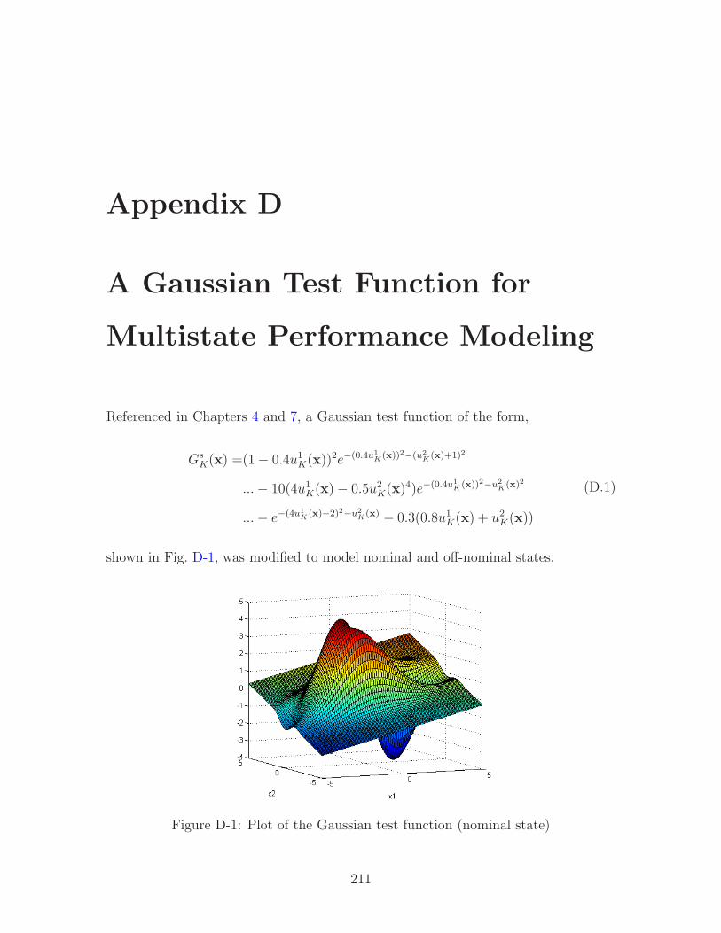
Appendix D
A Gaussian Test Function for
Multistate Performance Modeling
Referenced in Chapters 4 and 7, a Gaussian test function of the form,
GsK(x) =(1− 0.4u1K(x))
2e−(0.4u1K(x))2−(u2
K(x)+1)2
...− 10(4u1K(x)− 0.5u2K(x)4)e−(0.4u1
K(x))2−u2K(x)2
...− e−(4u1K(x)−2)2−u2
K(x) − 0.3(0.8u1K(x) + u2K(x))
(D.1)
shown in Fig. D-1, was modified to model nominal and off-nominal states.
Figure D-1: Plot of the Gaussian test function (nominal state)
211
This was accomplished by defining uK as shown in Eqn. D.2:
uK(x) =
α1K 0
0 α2K
x1
x2
+
γ1K
γ2K
,
where αK =
1 + f
1− a− bc
K
,
and γK =
b+ e
b+ d/(1− c)
K
(D.2)
The ‘mode’ vector [a b c d e f ]K is defined as:
a
b
c
d
e
f
T
K
=
0.6
0.5
0.5
1.5
−1.5
1.4
T
{0, 1} 0 0 0 0 0
0 {0, 1} 0 0 0 0
0 0 {0, 1} 0 0 0
0 0 0 {0, 1} 0 0
0 0 0 0 {0, 1} 0
0 0 0 0 0 {0, 1}
K
(D.3)
The above equations model a multistate system with six modes of failure, cor-
responding to [a b c d e f ] and the diagonal elements of the right hand matrix in
Eqn. D.3. These diagonal elements are 0 when the represented element is functional
and 1 when it has failed. When the diagonal consists of all zeros, uK(x) = x, and the
function is in its ‘nominal’ state as displayed in Fig. D-1. All of the other possible
permutations correspond to the 63 off-nominal states. These states are essentially
modeled by a shifting and stretching of the performance space via the mechanisms
in Eqns. D.2 and D.3. Plots of four ‘off-nominal’ states are shown in Figs. D-2
through D-5 on the following page. The starred points are representations of Kriging
surfaces mapped from the nominal state, as described in Chapter 7.
212

Figure D-2: Plot of the Gaussian test function (off-nominal with ‘a’ and ‘f’ failed)
Figure D-3: Plot of the Gaussian test function (off-nominal with ‘a’ ‘b’ and ‘c’ failed)
213

Figure D-4: Plot of the Gaussian test function (off-nominal with ‘e’ and ‘f’ failed)
Figure D-5: Plot of the Gaussian test function (off-nominal with ‘a’ ‘d’ and ‘f’ failed)
214
Appendix E
Multistate Modeling for the Long
Endurance UAV
The multistate performance model for both scenarios of the long endurance UAV
generally executes according to the iterative processes given in Fig. 5-6, of Chapter 5.
The modules used to define the aircraft are similar to those used in the twin-engine
aircraft model, but with the mass properties module being updated to reflect current
technology used in lighter weight, high aspect ratio UAVs. These corrections were
made according to the mass data given in the NASA study of [83]. The modeling of
thrust and energy consumption was also adjusted accordingly, depending on whether
the aircraft was using traditional combustible fuel or the LH2-PEM fuel cells.
The trim algorithm represented by the innermost loop of Fig. 5-6 was constructed
using the methods found in a very early, but extremely thorough, publication of
Roskam [90], and in Grasmeyer [51]. The Grasmeyer publication was a NASA study,
contracted in 1998, to determine engine-out constraints based on estimation of sta-
bility and control derivatives. These derivatives can be used in the characterization
an aircraft’s equilibrium about or along any one of its axes, such as that in Eqn. E.1,
Cyδaδa + Cyδr
δr + Cyββ + CLsin φ− Tsin ε
qS= −Yext
qS(E.1)
which is the sideforce equation, derived from the 6-DoF equations of motion, as found
215
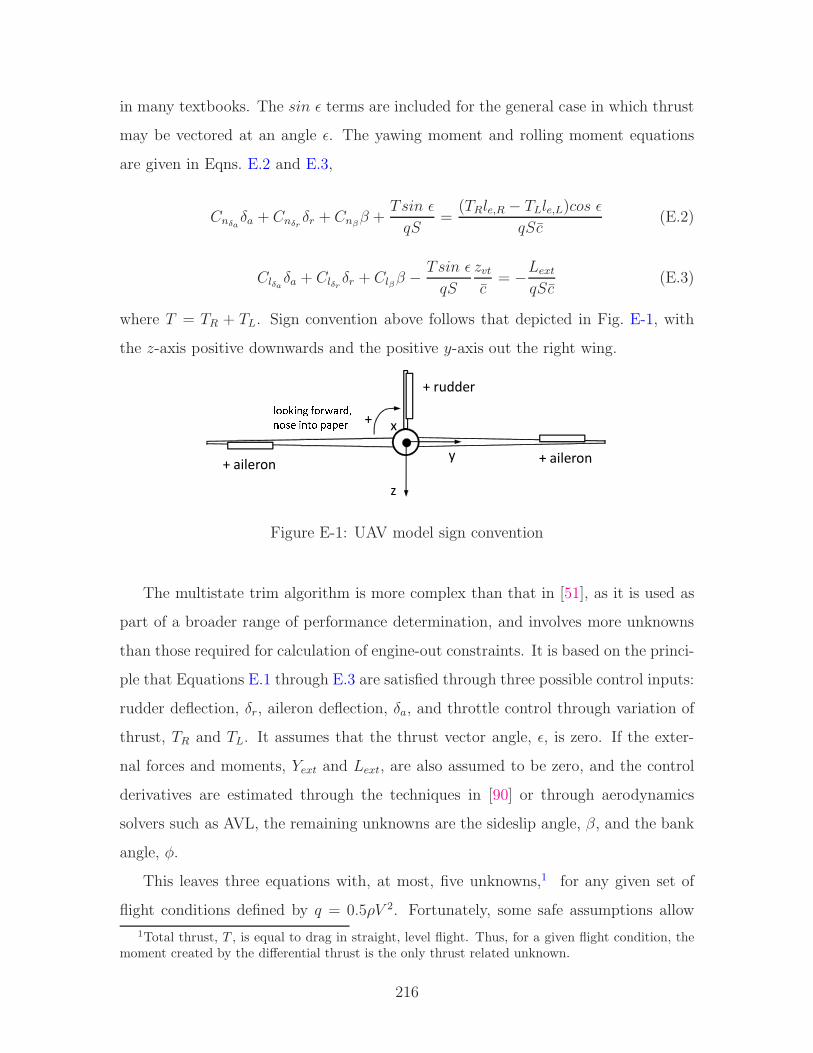
in many textbooks. The sin ε terms are included for the general case in which thrust
may be vectored at an angle ε. The yawing moment and rolling moment equations
are given in Eqns. E.2 and E.3,
Cnδaδa + Cnδr
δr + Cnββ +
Tsin ε
qS=
(TRle,R − TLle,L)cos ε
qSc(E.2)
Clδaδa + Clδr
δr + Clββ − Tsin ε
qS
zvtc
= −Lext
qSc(E.3)
where T = TR + TL. Sign convention above follows that depicted in Fig. E-1, with
the z-axis positive downwards and the positive y-axis out the right wing.
y
z
x++ rudder
+ aileron+ aileron
+,,-./0 1,234256/,78 ./9, :4:82Figure E-1: UAV model sign convention
The multistate trim algorithm is more complex than that in [51], as it is used as
part of a broader range of performance determination, and involves more unknowns
than those required for calculation of engine-out constraints. It is based on the princi-
ple that Equations E.1 through E.3 are satisfied through three possible control inputs:
rudder deflection, δr, aileron deflection, δa, and throttle control through variation of
thrust, TR and TL. It assumes that the thrust vector angle, ε, is zero. If the exter-
nal forces and moments, Yext and Lext, are also assumed to be zero, and the control
derivatives are estimated through the techniques in [90] or through aerodynamics
solvers such as AVL, the remaining unknowns are the sideslip angle, β, and the bank
angle, φ.
This leaves three equations with, at most, five unknowns,1 for any given set of
flight conditions defined by q = 0.5ρV 2. Fortunately, some safe assumptions allow
1Total thrust, T , is equal to drag in straight, level flight. Thus, for a given flight condition, themoment created by the differential thrust is the only thrust related unknown.
216

the extra two unknowns to be computationally solved for through iteration. The first
assumption is that the smallest possible control surface deflection should be used to
counter any moments generated by engine loss. This accounts for the first unknown,
allowing alternate iteration on δr and δa for a fixed thrust differential, starting from
zero degrees and stopping when the force and moment equations are satisfied, or max
deflections have been reached.
The second assumption is that for the above aircraft, trimmed using control sur-
faces, any beneficial reduction in the thrust differential must result in a higher cruise
altitude. Figure E-2 shows this trend for the state with an inoperative inboard engine
and failed rudder.
40 50 60 70 80 90 1003.7
3.8
3.9
4
4.1
4.2
4.3
4.4
4.5x 10
4
Throttle setting on engines opposite failed engine [%]
Bes
t cr
uise
alti
tude
[ft
]
↓D;<=>> ↓T↓D;<=>< ↓T
?@ABC DEEF GABCHAGEIJCBK@LB ACGMMBK HGCLCHNAAOCEAADB PBAAGIQ @IAGDHDAGA@KB PAEFP GILCBHPGIQFigure E-2: Variation of best cruise altitude (at end of cruise-climb) with throttlesetting for aircraft with failed inboard engine and rudder
The optimum throttle setting in Fig. E-2 arises from the fact that the flight
conditions entering the trim algorithm are those for minimum power required at
altitude (found by solving Eqn. 5.2, in Chapter 5). In other words, every point on the
throttle-altitude line is constrained by Eqn. 5.2. Throttle reduction of the operating
217
engines must be accompanied by a reduction in trim drag greater in magnitude than
the resulting loss in total thrust, in order to be ‘improving.’ Given the constraint
of Eqn. 5.2, this will show up as an increase in cruise altitude, when reducing from
100% throttle. Therefore, the complete trim process is to inner loop iterate on control
deflections (increasing) until moments are zero, and outer loop iterate on throttle
(decreasing) until cruise altitude stops increasing. This results in the best trimmed
cruise performance for the engine-out scenario.
In practice, there is one additional iteration that occurs between the inner and
outer loops discussed above. This is an iteration on altitude required to satisfy
Eqn. 5.2, which is a function of both a Mach number and altitude. The solution
to this is to select a low altitude, solve for the Mach number required to satisfy
Eqn. 5.2, shown below in Eqn. E.4,
Mcr =
√2W√
ρS(aπeA3CDo)
(E.4)
and then increase altitude incrementally until the design required Mach number at
altitude is reached, or thrust becomes limited at altitude.2 The implicit result is that
every performance output is already calculated at the best possible cruise conditions,
corresponding to the minimum power required and the highest altitude.
Sample results for the baseline long endurance UAV are provided in Fig. E-3 and
Fig. E-4. Although spread across separate figures on two pages, they compose a single
design point for 64 states. The deflection, sideslip, and bank angles are those required
to trim the aircraft in the appropriate engine-out scenario.
2Both density, ρ, and the speed of sound, a, are decreasing functions of altitude. Since they arelocated in the denominator of Eqn. E.4, the best cruise Mach number increases with altitude.
218
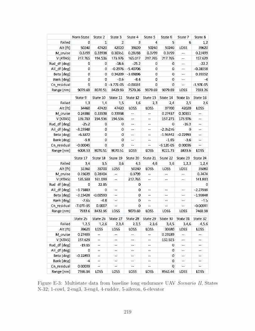
RSTUVWVX UVWVX Y UVWVX Z UVWVX [ UVWVX \ UVWVX ] UVWVX ^ UVWVX _`WabXc d e Y Z [ \ ] efYgbV hiVj \dY[d [ [Yd [YdYd Zk_Yd \dY[d \dY[d lmUU Zk]YdnopqrasX dtZ^kk dtZZkZ_ dtZdZ\e dtY_^__ dtZ^kk dtZ^kk uu dtY [kkv hwxgUj Ye t^]\ ek[t\Z] e Ztk^] e]\tde^ Ye^t^]\ Ye^t^]\ uu e\^t]Ykyrcoci hcXzj d d ue_t] uY\tY d d uu uYYtYgaboci hcXzj d d udtYk^] u\t[d^d] d d uu udtY_\\_{XVW hcXzj d d dtZ[Ydk uZt]k_k] d d uu dtZ\\\Y{W|} hcXzj d d uZt] u_t[ d d uu u[~|oqXsacrWb d d uZt^^�ud\ udtdddZe d d uu uetk^�ud\yW|zX h|Tj kd^kt]k _d^dt\e _[YktkZ ^\^dtZ] kd^kt]k kd^kt]k lmUU ^\kZtY]UVWVX k UVWVX ed UVWVX ee UVWVX eY UVWVX eZ UVWVX e[ UVWVX e\ UVWVX e]`WabXc efZ ef[ ef\ ef] YfZ Yf[ Yf\ Yf]gbV hiVj Z[[]d [ [Yd [^[Yd lmUU lmUU Z^^dd [YdYd lmUUnopqrasX dtY[Z_] dtZZkZ_ dtZZkZ_ uu uu dtY^[Z^ dtZdZ\e uuv hwxgUj eZkt^_Z ek[t\Z] ek[t\Z] uu uu e\^tY^Z e^Ztk^] uuyrcoci hcXzj uY\tY d d uu uu d ue]tZ uugaboci hcXzj u_tYZk[_ d d uu uu uYtZ\Y^] d uu{XVW hcXzj u]tZZ^Y d d uu uu uetk][[Y udtYYkkZ uu{W|} hcXzj ukt_ d d uu uu uet]\ uZt] uu~|oqXsacrWb udtddd[\ d d uu uu u]teY�ud\ dtdddZ] uuyW|zX h|Tj ]dd_t\Z _d^dt\e _d^dt\e lmUU lmUU _YYet^Z _[ZZt] lmUUUVWVX e^ UVWVX e_ UVWVX ek UVWVX Yd UVWVX Ye UVWVX YY UVWVX YZ UVWVX Y[`WabXc Zf[ Zf\ Zf] [f\ [f] \f] efYfZ efYf[gbV hiVj ZeZ]d Z_^dd lmUU \dY[d lmUU lmUU lmUU Z\d_dnopqrasX dtYZ]Zk dtY_ed[ uu dtZ^kk uu uu uu dtY[^[v hwxgUj eZ\t\dZ e]etdkk uu Ye t^]\ uu uu uu e[et_eZyrcoci hcXzj d uYYt_\ uu d uu uu uu dgaboci hcXzj uZt^Z__Z d uu d uu uu uu uYtY^ke]{XVW hcXzj uZte\[Y_ udtdY\kZ uu d uu uu uu uetkZ_[_{W|} hcXzj uYt]\ u[t_ uu d uu uu uu uet\~|oqXsacrWb u^td^�ud\ dtddd^ uu d uu uu uu udtdddeeyW|zX h|Tj ^kZZt] _[ZYtk] lmUU kd^kt]k lmUU lmUU lmUU ^[]_tk_UVWVX Y\ UVWVX Y] UVWVX Y^ UVWVX Y_ UVWVX Yk UVWVX Zd UVWVX Ze UVWVX ZY`WabXc efYf\ efYf] YfZf[ YfZf\ YfZf] Zf[f\ Zf[f] [f\f]gbV hiVj Zk]Yd lmUU lmUU lmUU lmUU Zd]_d lmUU lmUUnopqrasX dtY^[kk uu uu uu uu dtYZe_k uu uuv hwxgUj e\^t]Yk uu uu uu uu eZYtkYZ uu uuyrcoci hcXzj uekt_\ uu uu uu uu d uu uugaboci hcXzj d uu uu uu uu d uu uu{XVW hcXzj udtYY_kZ uu uu uu uu d uu uu{W|} hcXzj u[ uu uu uu uu d uu uu~|oqXsacrWb dtdddZk uu uu uu uu d uu uuyW|zX h|Tj ^\k]t_[ lmUU lmUU lmUU lmUU _\]Yt[[ lmUU lmUUFigure E-3: Multistate data from baseline long endurance UAV Scenario II, StatesN-32; 1-cowl, 2-eng3, 3-eng4, 4-rudder, 5-aileron, 6-elevator
219
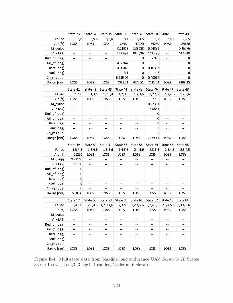
����� �� ����� �� ����� �� ����� �� ����� �� ����� �� ����� �� ����� �������� ����� ����� ����� ����� ����� ����� ����� �������� ���� ���� ���� ���� ����� ����� ����� ���� ������������� �� �� �� � ����� � ����� � ����� �� � �����¡ �¢£��� �� �� �� ��� ��� ��� ��� ��� ��� �� ��� ���¤����� ���¥� �� �� �� � � ��� � �� ������� ���¥� �� �� �� �� ����� � � �� �¦��� ���¥� �� �� �� �� ����� � �� ����� �� �¦�§¨ ���¥� �� �� �� �� � � �� � �� �©§��������� �� �� �� �� ��ª��� � � ����� �� �¤�§¥� �§«� ���� ���� ���� ���� �� ���� �� ���� �� ���� ���� ������� �� ����� �� ����� �� ����� �� ����� �� ����� �� ����� �� ����� �������� ����� ����� ������� ������� ������� ������� ������� ���������� ���� ���� ���� ���� ���� ���� ����� ���� ������������ �� �� �� �� �� � ����� �� ��¡ �¢£��� �� �� �� �� �� ��� ��� �� ��¤����� ���¥� �� �� �� �� �� � �� �������� ���¥� �� �� �� �� �� � �� ��¦��� ���¥� �� �� �� �� �� � �� ��¦�§¨ ���¥� �� �� �� �� �� � �� ��©§��������� �� �� �� �� �� � �� ��¤�§¥� �§«� ���� ���� ���� ���� ���� ���� �� ���� ��������� �� ����� �� ����� �� ����� �� ����� �� ����� �� ����� �� ����� �������� ������� ������� ������� ������� ������� ������� ������� ���������� ���� ����� ���� ���� ���� ���� ���� ���� ������������ � ����� �� �� �� �� �� �� ��¡ �¢£��� ��� �� �� �� �� �� �� �� ��¤����� ���¥� � �� �� �� �� �� �� �������� ���¥� � �� �� �� �� �� �� ��¦��� ���¥� � �� �� �� �� �� �� ��¦�§¨ ���¥� � �� �� �� �� �� �� ��©§��������� � �� �� �� �� �� �� ��¤�§¥� �§«� ���� �� ���� ���� ���� ���� ���� ���� ��������� �� ����� �� ����� �� ����� �� ����� �� ����� �� ����� �� ����� �������� ������� ��������� ��������� ��������� ��������� ��������� ����������������������� ���� ���� ���� ���� ���� ���� ���� ���� ������������ �� �� �� �� �� �� �� ��¡ �¢£��� �� �� �� �� �� �� �� ��¤����� ���¥� �� �� �� �� �� �� �� �������� ���¥� �� �� �� �� �� �� �� ��¦��� ���¥� �� �� �� �� �� �� �� ��¦�§¨ ���¥� �� �� �� �� �� �� �� ��©§��������� �� �� �� �� �� �� �� ��¤�§¥� �§«� ���� ���� ���� ���� ���� ���� ���� ����Figure E-4: Multistate data from baseline long endurance UAV Scenario II, States33-64; 1-cowl, 2-eng3, 3-eng4, 4-rudder, 5-aileron, 6-elevator
220
Bibliography
[1] J. Agte, N. Borer, and O. de Weck. Multistate design approach to the anal-ysis of performance robustness for a twin-engine aircraft. Journal of Aircraft(recommended for publication pending minor revisions), March 2011. 38, 176
[2] J. Agte and K. Cohen. First order effects of new technology on a high altitudelong endurance (HALE) unmanned aerial vehicle (UAV). In Proceedings of the46th AIAA Aerospace Sciences Meeting and Exhibit, Reno, Nevada, 2008. 124,132, 136
[3] J. Agte, O. de Weck, J. Sobieski, P. Arendsen, A. Morris, and M. Spieck. MDO:assessment and direction for advancement – an opinion of one internationalgroup. Structural and Multidisciplinary Optimization, 40(1):17–33, 2010. 49,50
[4] N. Alexandrov. Editorial - multidisciplinary design optimization. Optimizationand Engineering, 6(1):5–7, 2005. 49
[5] D. F. Allinger, P. S. Babcock, and R. F. LaPrad. The role of time-limiteddispatch operation in fault tolerant flight critical control systems. AGARDAdvisory Report No. 281, May 1990. 184
[6] C. Almeder. A hybrid optimization approach for multi-level capacitated lot-sizing problems. European Journal of Operational Research, 200(2):599–606,2010. 51
[7] P. J. Antsaklis and A. J. Michel. A Linear Systems Primer. Birkhauser, Boston,MA, 2007. 204
[8] AVL. Athena vortex lattice solver. http://web.mit.edu/drela/Public/web/avl/,Accessed July 2011. 72, 193
[9] P. S. Babcock IV. Channelization: the two-fault tolerant attitude control func-tion for the space station freedom. Aerospace and Electronics Systems Magazine(IEEE), 11(5):9–22, 1996. 32, 47, 77
[10] P. S. Babcock IV, G. Rosch, and J. J. Zinchuk. An automated environmentfor optimizing fault-tolerant systems designs. In Proceedings of the (1991) An-nual Reliability and Maintainability Symposium (IEEE), pages 360–367, Jan-uary 1991. 48
221

[11] P. S. Babcock IV and J. J. Zinchuk. Fault-tolerant design optimization: Appli-cation to an underwater vehicle navigation system. In Proceedings of the (1990)Symposium on Autonomous Underwater Vehicle Technology (IEEE/OES),pages 34–43, June 1990. 47
[12] R. J. Balling and J. Sobieszczanski-Sobieski. Optimization of coupled systems:A critical overview of approaches. AIAA Journal, 34(1):6–17, 1996. 50
[13] J. W. Bandler, Q. X. Cheng, S. A. Dakroury, A. S. Mohamed, M. H. Bakr,K. Madsen, and J. Sondergaard. Space mapping - the state of the art. IEEETransactions on Microwave Theory and Techniques, 52(1):337–361, 2004. 188
[14] J. W. Bandler, A. S. Mohamed, M. H. Bakr, K. Madsen, and J. Sondergaard.EM-based optimization exploiting partial space mapping and exact sensitivities.IEEE Transactions on Microwave Theory and Techniques, 50(12):2741–2750,2002. 188
[15] A. Banks, J. Vincent, and C. Anyakoha. A review of particle swarm opti-mization. part ii: hybridisation, combinatorial, multicriteria and constrainedoptimization, and indicative applications. Natural Computing, 7(1):109–204,2008. 51
[16] R. E. Barlow and A. S. Wu. Coherent systems with multi-state components.Mathematics of Operations Research, 3(4):275–281, 1978. 44
[17] J. F. M. Barthelemy and J. Sobieszczanski-Sobieski. Optimum sensitivityderivatives of objective functions in nonlinear programming. AIAA Journal,21:913–915, 1983. 51
[18] J. Berndt and A. de Marco. Progress on and usage of the open source flightdynamics model software library, JSBSim. In Proceedings of the (2009) AIAAModeling and Simulation Technologies Conference, August 2009. 72, 176, 194
[19] J. S. Berndt. JSBSim Reference Manual.http://jsbsim.sourceforge.net/JSBSimReferenceManual.pdf, AccessedJuly 2011. 196
[20] U. N. Bhat and G. K. Miller. Elements of Applied Stochastic Processes. JohnWiley and Sons, Inc., Hoboken, NJ, 2002. 59
[21] L. Blackmore. Robust Execution for Stochastic Hybrid Systems. PhD disser-tation, Massachusetts Institute of Technology, Department of Aeronautics andAstronautics, 2007. 31, 47
[22] W. R. Blischke and D. N. P. Murthy. Reliability - Modeling, Prediction, andOptimization. Wiley, New York, 2000. 54
222
[23] N. K. Borer, I. R. Claypool, W. D. Clark, J. J. West, R. G. Odegard, K. M.Somervill, and N. H. Suzuki. Model-driven development of reliable avionicsarchitectures for lunar surface systems. Technical report, IEEE AerospaceConference, Big Sky, Montana, March 2010. 77
[24] J. Braman, R. Murray, and D. Wagner. Safety verification of a fault tolerantreconfigurable autonomous goal-based robotic control system. In Proceedingsof the 2007 IEEE/RSJ International Conference on Intelligent Robots and Sys-tems, October 2007. 47
[25] S. A. Brandt, R. J. Stiles, J. J. Bertin, and R. Whitford. Introduction to Aero-nautics: A Design Perspective, second edition. American Institute of Aeronau-tics and Astronautics, Reston, VA, 2004. 71, 87, 129, 192, 193
[26] F. W. Burcham and C. G. Fullerton. Controlling crippled aircraft - with throt-tles. NASA/TM-104238, 1991. 46
[27] F. W. Burcham, T. A. Maine, C. G. Fullerton, and L. D. Webb. Developmentand flight evaluation of an emergency digital flight control system using onlyengine thrust on an F-15 airplane. Technical report, NASA, Edwards, CA,September 1996. 46
[28] J. P. Castro, G. A. Gray, A. Giunta, and P. D. Hough. Developing a compu-tationally efficient dynamic multilevel hybrid optimization scheme using mul-tifidelity model interactions. SAND2005-7498, Sandia National Laboratories,2005. 188
[29] K. Chang. Panel wants deep space, not landings as U.S. goal. The New YorkTimes, page A16, July 31, 2009. 27
[30] A. Cozzola and J. L. Dolce. High-altitude, long-endurance airships for coastalsurveillance. NASA/TM-2005-213427, February 2005. 27
[31] N. A. Creech, T. A. Burton, P. Cuadra, A. D. Harder, R. L. Odom, and J. S.Wisecup. C-12C parameter estimation, USAF TPS Technical Information Mem-orandum. Technical report, U.S. Air Force Test Pilot School, Edwards AFB,CA, March 2010. 74, 87
[32] DARPA. Broad Agency Announcement (BAA) Vulture II. Defense AdvancedResearch Projects Agency TTO, October 2009. 26, 78
[33] I. Das and J. Dennis. Normal-boundary intersection - a new method for gener-ating pareto optimal points multicriteria optimization problems. SIAM Journalon Optimization, 8(3):631–657, 1998. 104, 173
[34] O. de Weck and K. Willcox. Introduction to multidisciplinary system designoptimization. Lesson 1 Lecture Notes - Course 16.888, Spring 2010. 52
223

[35] Department of Defense. Military standard: Procedures for performing a failuremode, effects and criticality analysis. MIL-STD-1629A, November 1980. 98
[36] Department of Transport. The status of commercial passenger operations inturbine powered single engine aeroplanes. Technical report, Australian Bureauof Air Safety Investigation, Information Paper SAB/IP/93/4, December 1993.27, 83
[37] Department of Transportation. Hawker Beechcraft Model 200 Type CertificateData Sheet No. A24CE. Technical report, Federal Aviation AdministrationRegulatory and Guidance Library, March 2002. 73, 192, 193
[38] DoD. Acquisition strategy guide, 4th edition. Technical report, Defense SystemsManagement College Press, Fort Belvoir, VA, 1999. 96
[39] A. D. Dominguez-Garcia. An Integrated Methodology for the Performanceand Reliability Evaluation of Fault-Tolerant Systems. PhD dissertation, Mas-sachusetts Institute of Technology, Department of Electrical Engineering andComputer Science, May 2007. 32, 48
[40] A. D. Dominguez-Garcia, J. G. Kassakian, J. E. Schindall, and J. J. Zinchuk. Anintegrated methodology for the dynamic performance and reliability evaluationof fault-tolerant systems. Journal of Reliability Engineering and System Safety,93(11):1628–1649, 2008. 48
[41] Dov Dori. Object-Process Methodology: a Holistic Systems Paradigm. Springer,2002. 36
[42] G. Dorini. Performing pareto set membership tester for sets of points in k-dimensions. Matlab File Exchange, June 2007. 137
[43] M. A. Dornheim. Research pilot devises rules of thumb for engine-only controlof disabled aircraft. Aviation Week and Space Technology, page 43, June 24,1991. 46
[44] J. Dubbeldam and F. Redig. Multilayer markov chains with applications topolymers in shear flow. Journal of Statistical Physics, 125(1):229–247, 2006.105
[45] J. Dugan, S. Bavuso, and M. Boyd. Dynamic fault fault-tree models for fault-tolerant computer systems. IEEE Transactions on Reliability, 41(3):363–377,1992. 48
[46] D. Dvorak, M. Indictor, M. Ingham, R. Rasmussen, and M. Stringfellow. Aunifying framework for systems modeling, control systems design, and systemoperation. In Proceedings of the IEEE Conference on Systems, Man, and Cy-bernetics, October 2005. 46
224
[47] E. El-Neweihi, F. Proschan, and J. Sethuraman. Multistate coherent systems.Journal of Applied Probability, 15(4):675–688, 1978. 44
[48] A. Elfes, S. S. Bueno, M. Bergerman, E. C. de Paiva, and J. G. Ramos Jr.Robotic airships for exploration of planetary bodies with an atmosphere: Au-tonomy challenges. Autonomous Robots, 14(2-3):147–164, March 2003. 27
[49] FAA. Policy for time limited dispatch (TLD) of engines with full authority digi-tal engine controls (FADEC) systems. FAA Policy Letter ANE-1993-33.28TDL-R1, June 2001. 184
[50] F. Z. Feng, Y. H. Kim, and B. Yang. Applications of hybrid optimizationtechniques for model updating of rotor shafts. Structural and MultidisciplinaryOptimization, 32(1):65–75, 2006. 51
[51] J. Grasmeyer. Stability and control derivative estimation and engine-out anal-ysis. VPI-AOE-254, Virginia Tech, January 1998. 131, 215, 216
[52] R. T. Haftka and H. Adelman. Recent developments in structural sensitivityanalysis. Structural and Multidisciplinary Optimization, 1:137–151, 1989. 51
[53] Headquarters Department of the Army. Operator’s manual for Army C-12C/D/T aircraft. Technical report, Department of the Army, available atemilitarymanuals.com, September 2001. 73
[54] A. S. Hedayat, N. J. A. Sloane, and J. Stufken. Orthogonal Arrays - Theoryand Applications. Springer, New York, NY, 1999. 51, 103, 149
[55] R. A. Howard. Dynamic Probabilistic Systems: Volume I, Markov Models.Dover Publications, 2007. 60
[56] A. Hoyland and M. Rausand. System Reliability Theory. John Wiley and Sons,New York, NY, 1994. 48
[57] Moire Inc. Cost and business model analysis for civilian UAV missions. preparedfor the National Aeronautics and Space Administration, NASA, 2004. 132
[58] M. D. Ingham, R. D. Rasmussen, M. B. Bennett, and A. C. Moncada. Engi-neering complex embedded systems with state analysis and the mission datasystem. AIAA Journal of Aerospace Computing, Information and Communica-tion, 2(12):507–536, 2005. 46
[59] T. Jin, L. Xing, and Y. Yu. A hierarchical markov reliability model for datastorage systems with media self-recovery. International Journal of Reliability,Quality & Safety Engineering, 18(1):25–41, 2011. 105
[60] A. Mishkin R. Rasmussen T. Starbird J.R. Morris, M. Ingham. Application ofstate analysis and goal-based operations to a MER mission scenario. AIAA
2006-5981, AIAA International Conference on Space Operations, Rome, Italy,June 2006. 46
225
[61] I. Y. Kim and O. L. de Weck. Adaptive weighted-sum method for multi-objective optimization - a new method for Pareto front generation. Structuraland Multidisciplinary Optimization, 31(2):105–116, 2006. 104
[62] J. P. C. Kleijnen. Design and Analysis of Simulation Experiments. Springer,New York, NY, 2010. 51, 103, 137
[63] G. Kreisselmeier and R. Steinhauser. Systematic control design by optimizatinga vector performance index. In Proceedings of the International Federationof Active Controls Symposium on Computer-Aided Design of Control Systems,Zurich, Switzerland, 1979. 116
[64] J. Kurzke. Gasturb11 for design performance of gas turbine engines. Software,GasTurb11 Laboratory Package, 2009. 161
[65] G. Labinaz, M. M. Bayoumi, and K. Rudie. A survey of modeling and controlof hybrid systems. Annual Reviews in Control, 21(1):79–92, 1997. 47
[66] NASA Jet Propulsion Laboratory. Mission data system - state analysis.http://mds.jpl.nasa.gov/, accessed July 2011. 31, 46
[67] G. Levitin and A. Lisnianski. A new approach to solving problems of multi-state system reliability optimization. Quality and Reliability Engineering Inter-national, 17(2):93–104, 2001. 44, 66
[68] H. Li and B. C. Williams. Generalized conflict learning for hybrid discrete/linearoptimization. In Proceedings of the 11th International Conference on Principlesand Practices of Constraint Programming (CP-05), pages 415–429, September2005. 47
[69] A. Lisnianski and G. Levitin. Multi-State System Reliability, volume 6 of Serieson Quality, Reliability & Engineering Statistics. World Scientific, Singapore,2003. 31, 45, 54, 55, 59, 112
[70] A. Lisnianski, G. Levitin, H. Ben-Haim, and D. Elmakis. Power system struc-ture optimization subject to reliability contraints. Electric Power Systems Re-search, 39(2):145–152, 1996. 45
[71] F. J. Malzacher, J. Gier, and F. Lippl. Aerodesign and testing of an aerome-chanically highly loaded lp turbine. Journal of Turbomachinery, 128(4):643–649,2006. 156
[72] K. F. Man, K. S. Tang, and S. Kwong. Genetic Algorithms: Concepts andDesign, 3rd Edition. Springer-Verlag, London, United Kingdom. 51
[73] Y. Massim, A. Zeblah, R. Meziane, M. Benguediab, and A. Ghouraf. Optimaldesign and reliability evaluation of multi-state series-parallel power systems.Nonlinear Dynamics, 40(4):309–321, 2005. 45
226
[74] J. Matson. Unfree spirit - NASA’s mars rover appears stuck for good. ScientificAmerican, 302(4):16, March 2010. 26
[75] A. Mettas. Reliability allocation and optimization for complex systems. InProceedings of the Annual IEEE Reliability and Maintainability Symposium,Los Angeles, CA, January 2000. 132
[76] Brian Mills. DIY Drones: Profile of Brian Mills.http://diydrones.ning.com/profile/BrianMills, Accessed July 2011.72, 194
[77] J. D. Murchland. Fundamental Concepts and Relations for Reliability Analysisof Multistate Systems. Reliability and Fault Tree Analysis, Theoretical, andApplied Aspects of System Reliability. SIAM, 1975. 44
[78] NASA. NASA Systems Engineering Handboook. NASA Center for AerospaceInformation, Hanover, MD, 2007. 96
[79] NASA. Icebridge: an airborne mission for earth’s polar ice.http://www.nasa.gov/mission_pages/icebridge/, Accessed July 2011.123
[80] NASA. ICESat - cryoshperic sciences. http://icesat.gsfc.nasa.gov/icesat/,Accessed July 2011. 122
[81] National Transportation Safety Board. Annual review of aircraft accident data- U.S. air carrier operations calendar year 2006. Technical report, NTSB/ARC-10/01, December 2006. 27, 83
[82] US Navy. NAVAIR acquisition guide. Technical report, Department of Defense,2009. 96
[83] C. L. Nickol, M. D. Guynn, L. L. Kohout, and T. A. Ozoroski. High alti-tude long endurance uav analysis of alternatives and technology requirementsdevelopment. NASA/TP-2007-214861, March 2007. 124, 136, 215
[84] Office of the Secretary of Defense. Unmanned aerial vehicle reliability study.Technical report, Department of Defense, Washington, D.C., February 2003.27, 83, 125, 126, 127
[85] V. Pareto and S. Schwier. Manual of Politcal Economy. Kellag, New York, NY,1971. 103
[86] D. P. Raymer. Aircraft Design: A Conceptual Approach, third edition. AmericanInstitute of Aeronautics and Astronautics, Reston, VA, 1999. 131, 194
[87] A. Reibman and M. Veeraraghavan. Reliability modeling: An overview forsystem designers. IEEE Computer, 24(4):49–57, 1991. 48
227

[88] C. Riegler and C. Bichlmaier. The geared turbofan technology opportunities,challenges, and readiness status. In Proceedings of the 1st CEAS European Airand Space Conference, Berlin, Germany, September 2007. 156
[89] H. H. Rosenbrock. State-space and Multivariable Theory. Wiley InterscienceDivision, New York, NY, 1970. 204
[90] J. Roskam. Methods for Estimating Stability and Control Derivatives of Con-ventional Subsonic Airplanes. Roskam Aviation and Engineering Corporation,Kansas, 1971. 131, 215, 216
[91] J. Roskam. Airplane Design Part VI. Roskam Aviation and Engineering Corp.,Ottawa, KS, 1990. 194
[92] J. Roskam. Airplane Design Part VIII. Roskam Aviation and EngineeringCorp., Ottawa, KS, 1990. 71, 192
[93] R. A. Rutenbar. Simulated annealing algorithms: An overview. IEEE Circuitsand Devices Magazine, 5(1):19–26, 1989. 51
[94] P. S. Schenker, P. Pirjanian, B. Balaram, K. S. Au, A. Trebi-Ollennu, T. L.Huntsberger, H. Aghazarian, B. A. Kennedy, E. T. Baumgartner, K. lagnemma,A. Rzepniewski, S. Dubowsky, P. C. Leger, D. Apostolopoulos, and G. T. Mc-Kee. Reconfigurable robots for all terrain exploration. Proceedings of SPIE,4196(2000):454–468, 2000. 27
[95] K. Sinha, D. James, and J. Agte. Multidisciplinary design optimization of ahigh bypass ratio geared turbofan engine. Final report - Course 16.888, Mas-sachusetts Institute of Technology, Cambridge, MA, May 2010. 156
[96] M. Smotherman and K. Zemoudeh. A non-homogeneous markov modelfor phased-mission reliability analysis. IEEE Transactions on Reliability,38(5):585–590, December 1989. 48
[97] J. Sobieszczanski-Sobieski. Sensitivity of complex, internally coupled systems.AIAA Journal, 28(1):153–160, 1990. 51
[98] J. Sobieszczanski-Sobieski and R. T. Haftka. Multidisciplinary aerospace designoptimization: survey of recent developments. Structural and MultidisciplinaryOptimization, 14(1):1–23, 1997. 49
[99] M. Stein. Interpolation of Spatial Data - Some Theory for Kriging. Springer,New York, 1999. 186
[100] M. Steinberg. Historical overview of research in reconfigurable flight control.Proceedings of the Institution of Mechanical Engineers, 219(4):263–275, 2005.45
228

[101] B. L. Stevens and F. L. Lewis. Aircraft Control and Simulation. Wiley Inter-science Division, New York, NY, 1992. 205
[102] D. V. Stewart. The design structure matrix - a method for managing thedesign of complex systems. IEEE Transactions on Engineering Management,28(3):71–74, 1981. 51
[103] T. Ozoroski, M. Guynn, and C. Nickol. Quick look feasibility study for anunmanned aerial vehicle ice surveillance mission. NASA viewgraphs, NASALangley Research Center, June 2007. 123
[104] H. A. Taboada, J. F. Espiritu, and D. W. Coit. MOMS-GA: A multi-objectivemulti-state genetic algorithm for system reliability optimization design prob-lems. IEEE Transactions on Reliability, 24(1):182–191, 2008. 45
[105] N. P. Tedford and J. Martins. On the common structure of MDO problems: acomparison of architectures. AIAA 2006-7080, 11th AIAA/ISSMO Multidis-ciplinary Analysis and Optimization Conference, Portsmouth, VA, September2006. 49
[106] S. Thompson and J. Agte. C-12C aerodynamic model evaluation, USAF TPSMemorandum. Technical report, U.S. Air Force Test Pilot School, EdwardsAFB, CA, April 2001. 73
[107] J. Till, S. Engell, S. Panek, and O. Stursberg. Applied hybrid system optimiza-tion: An empirical investigation of complexity. Control Engineering Practice,12(10):1291–1303, 2004. 47
[108] M. Tozan, A. M. Al-Garni, A. Z. Al-Garni, and A. Jamal. Failure data analysisfor aircraft maintenance planning. In Proceedings of the 2004 Aircraft Engi-neering Symposium, Jeddah, Saudi Arabia, December 2004. 159
[109] S. Tsach, A. Peled, D. Penn, and D. Touitou. The CAPECON program: Civilapplications and economical effectivity of potential UAV configurations. In Pro-ceedings of the 3rd AIAA Unmanned Unlimited Technical Conference, Work-shop, and Exhibit, Chicago, Illinios, September 2004. 132
[110] I. Ushakov. The method of generalized generating sequences. European Journalof Operational Research, 125(2):675–688, 2000. 44
[111] D. G. Ward and J. F. Monaco. System identification for retrofit reconfigurablecontrol of an f/a-18 aircraft. Journal of Aircraft, 42(1):63–72, 2005. 46
[112] J. West, I. Claypool, N. Borer, and R. Odegard. LSS lunar habitat avionicsmodeling study - Task 3 final report, reliability and performance implications ofthe use of commercial grade components. NASA/JSC Contract NNJ06HC37C,Draper Laboratory, 2009. 132
229

[113] J. G. Ziegler and N. B. Nichols. Optimum settings for automatic controllers.Transactions of the A.S.M.E., 64:759–768, 1942. 80
230