Multisymplectic Geometry on theThree Dimensional

General Schrodinger Equation

Katheryn R. WhiteheadControl & Dynamical Systems

California Institute of TechnologyCourse: CDS 205

June 1, 2007

Abstract

A multisymplectic structure is imposed on the 3-d (three dimen-sional) general Schrodinger equation. From the multisymplectic formformula, a multisymplectic conservation law is extracted for the 3-dgeneral Schrodinger equation. For the case of infinite spatial domain,the multisymplectic form formula is shown to reduce to a form thatcoincides with the quantum-mechanical symplectic form, which is de-fined in terms of the imaginary part of the quantum mechanical Her-mitian inner product on the complex Hilbert space of square integrablewavefunctions. Furthermore, the interpretation of the multisymplecticform formula in application to the 3-d general Schrodinger equationwith infinite spatial domain and bounded time domain, is that theintegrals over the two boundaries at each temporal endpoint are equalin magnitude, and yet opposite in orientation.

1

Contents

1 Introduction 3

2 The General Schrodinger Equation 4

3 Geometrizing the General Schrodinger Equation 53.1 A Fiber Bundle Structure Imposed on the General Schrodinger

Equation . . . . . . . . . . . . . . . . . . . . . . . . . . . . . . 53.2 Multisymplectic Manifold / Covariant Phase Space . . . . . . 63.3 The Euler-Lagrange Equations . . . . . . . . . . . . . . . . . . 83.4 The Lagrangian Formulation Applied to the General Schrodinger

Equation . . . . . . . . . . . . . . . . . . . . . . . . . . . . . . 113.5 The Hamiltonian Formulation . . . . . . . . . . . . . . . . . . 113.6 The Hamiltonian Formulation Applied to Schodinger Equation 14

4 The Multisymplectic Structure 15

5 The Multisymplectic Form Formula 16

6 Conclusion 23

7 References 24

2

1 Introduction

In 1925, Erwin Schrodinger suggested that the Schrodinger equation wouldgovern the behavior of very small particles. The Schrodinger equation pro-vided the link between the motion of particles and their dependence on timeand spatial position, subject to forces external to the system. The time de-pendent and the time independent Schrodinger equation comes in variousforms depending on the system of application.

The part that differentiates one form of the Schrodinger equation fromanother can be seen in the quantum mechanical Hamiltonian operator. Thetype of system under study, and the type of information that is desired toattain, is what determines the form of the system’s Hamiltonian operatorthat will be employed by the Schrodinger equation. The free Hamiltonianoperator in its most basic sense comprises of a kinetic energy operator andsome type of potential energy operator. The potential energy function is de-pendent on the number of particles in the system of study, as well as the typeof particles under study, and what type of interaction these particles havewith one another. In addition, to the free Hamiltonian operator, a pertur-bation Hamiltonian is often added. For example, a magnetic field imposedonto a system of particles with intrinsic spin will introduce a perturbationHamiltonian to be added to the free Hamiltonian.

The goal of this paper is to set up the geometric structure in a mathe-matical sense, for the general three dimensional Schrodinger equation. Theterm ”general” in used in this paper in the sense that arbitary perturbationHamiltonians may be added to the free Hamiltonian, as long as perturbationsdepend only on space, time, and the wavefunction itself.

3

2 The General Schrodinger Equation

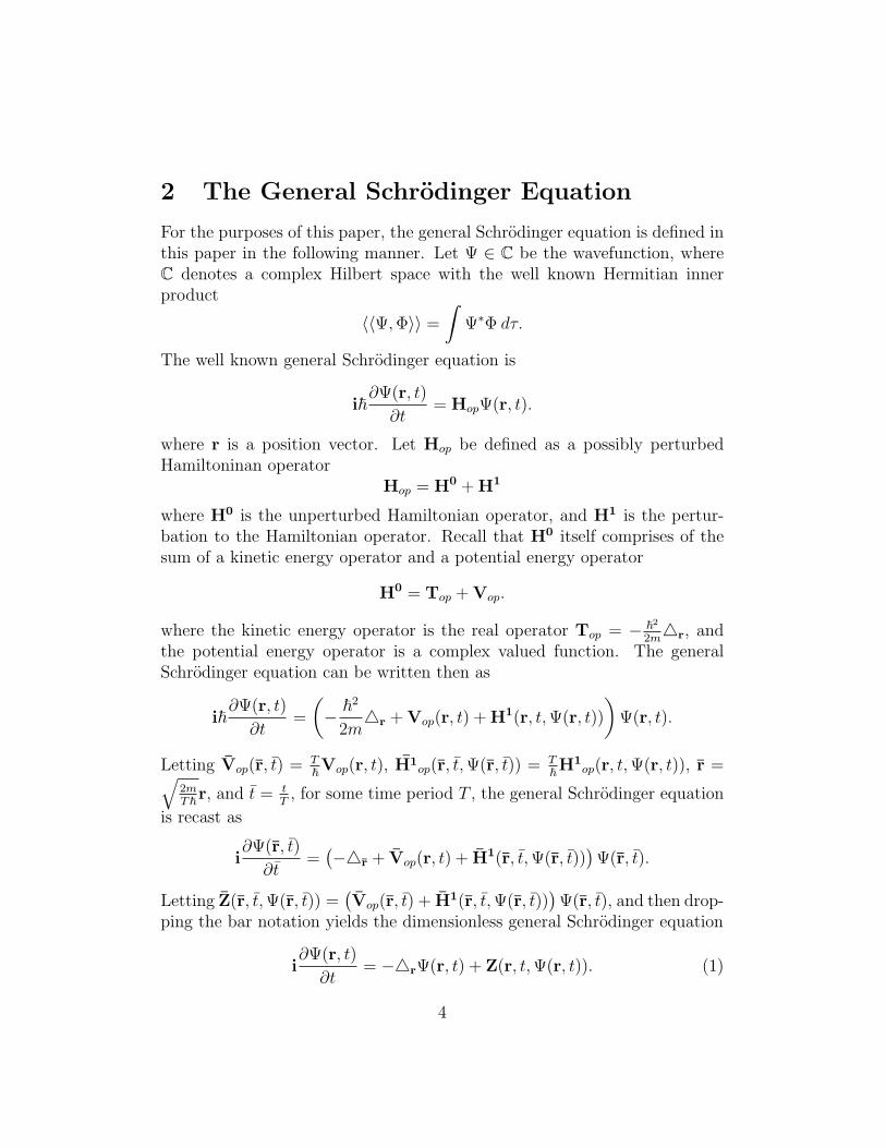
For the purposes of this paper, the general Schrodinger equation is defined inthis paper in the following manner. Let Ψ ∈ C be the wavefunction, whereC denotes a complex Hilbert space with the well known Hermitian innerproduct

〈〈Ψ, Φ〉〉 =

∫Ψ∗Φ dτ.

The well known general Schrodinger equation is

i~∂Ψ(r, t)

∂t= HopΨ(r, t).

where r is a position vector. Let Hop be defined as a possibly perturbedHamiltoninan operator

Hop = H0 + H1

where H0 is the unperturbed Hamiltonian operator, and H1 is the pertur-bation to the Hamiltonian operator. Recall that H0 itself comprises of thesum of a kinetic energy operator and a potential energy operator

H0 = Top + Vop.

where the kinetic energy operator is the real operator Top = − ~2

2m4r, and

the potential energy operator is a complex valued function. The generalSchrodinger equation can be written then as

i~∂Ψ(r, t)

∂t=

(− ~2

2m4r + Vop(r, t) + H1(r, t, Ψ(r, t))

)Ψ(r, t).

Letting Vop(r, t) = T~ Vop(r, t), H1

op(r, t, Ψ(r, t)) = T~ H1

op(r, t, Ψ(r, t)), r =√2mT~ r, and t = t

T, for some time period T , the general Schrodinger equation

is recast as

i∂Ψ(r, t)

∂t=

(−4r + Vop(r, t) + H1(r, t, Ψ(r, t))

)Ψ(r, t).

Letting Z(r, t, Ψ(r, t)) =(Vop(r, t) + H1(r, t, Ψ(r, t))

)Ψ(r, t), and then drop-

ping the bar notation yields the dimensionless general Schrodinger equation

i∂Ψ(r, t)

∂t= −4rΨ(r, t) + Z(r, t, Ψ(r, t)). (1)

4

Note that Z(r, t, Ψ(r, t)) takes values in the complex set of numbers, and isa function of time and spatial coordinates, as well as the wavefunction itself.

To facilitate geometrizing of the general Schrodinger equation, the imag-inary number i is eliminated from the equation by separating out the imag-inary and real part of the wavefunction. This is accomplished by lettingΨ(r, t) = p(r, t) + iq(r, t). Therefore equation 1 may be rewritten as

pt +4q − ImZ(r, t, p(r, t), q(r, t)) = 0qt −4p + ReZ(r, t, p(r, t), q(r, t)) = 0.

(2)

Please pay special attention to the fact that in general

ReZ(r, t, p(r, t), q(r, t)) 6= ReZ(r, t, Ψ(r, t))ImZ(r, t, p(r, t), q(r, t)) 6= ImZ(r, t, Ψ(r, t))

Now suppose there exists a function C such that

∂C∂p

= ReZ(r, t, p(r, t), q(r, t))∂C∂q

= ImZ(r, t, p(r, t), q(r, t)).

Consequently the equations in 2 become

pt +4q − ∂C∂q

= 0

qt −4p + ∂C∂p

= 0.(3)

Throughout this paper Cartesian coordinates will be utilized, and thus 4 =∂2

∂x+ ∂2

∂y+ ∂2

∂zfor r = (x, y, z).

3 Geometrizing the General Schrodinger Equa-

tion

3.1 A Fiber Bundle Structure Imposed on the GeneralSchrodinger Equation

Let πXY : Y → X be a fiber bundle over the oriented manifold X, andlet φ : U ⊂ X → Y be a section of πXY . For the three dimensional timedependent Schrodinger equation, the base space X of the fiber bundle is thespatial and time domain, and therefore is coordinated by xµ = (x, y, z, t),

5

where µ ∈ 1, . . . , (n + 1) = 4, and thus the dimesion of X is four. Thefibers over X are elements of Y , where Y is coordinated by the set yA (A ∈1, . . . , N), where for the general Schrodinger equation, these coordinatesare φ(x, y, z, t) = (p, q), and the dimension of Y is N = 2. The tangentmap of φ at k ∈ X, Tkφ, is an element of J1(Y )φ(k), where J1(Y ) is thefirst jet bundle over Y . Elements of J1(Y ), can be thought of as fibers overboth X and Y , and are defined to be the maps from TY to TX. The firstjet bundle J1(Y ) is coordinated by the set vA

µ , and thus the dimension ofJ1(Y ) is N ∗ (n+1). For the case of the general Schrodinger equation, J1(Y )is coordinated by (pt, qt, px, qx, py, qy, pz, qz), and the dimension of J1(Y ) isN ∗ (N + 1) = 2 ∗ 4 = 8.

The first jet, or first prolongation of φ, denoted by j1φ, is the map fromthe base space X to the first jet bundle J1(Y ). Note that j1(φ) ∈ Γ(πX,J1(Y ))is a section of J1(Y ). The coordinates of j1(φ) at a point k = xµ ∈ X are

j1k(φ) =

(xµ, φA(xµ),

∂φA(xµ)

∂xν

)For the 3-d (three dimensional) general Schrodinger equation, j1(φ) at a pointk = (x, y, z, t) ∈ X is

j1k(φ) = ((x, y, z, t), (p, q), (pt, qt, px, qx, py, qy, pz, qz)).

3.2 Multisymplectic Manifold / Covariant Phase Space

The dual jet bundle is denoted by J1(Y )?. The dual jet bundle consists ofthe set of affine maps from J1(Y ) to Λ(n+1)(X), where Λ(n+1)(X) is the set of(n+1)-forms on X (Recall that (n+1) is the dimension of the base space X).To define a multisymplectic manifold, first define the bundle of (n+1) formson Y , denoted by Λ := Λ(n+1)(Y ), with projection map πY Λ : Λ → Y . Anoteworthy subbundle of Λ is denoted by Z ⊂ Λ, and this subbundle consistsof the fibers

Zy = z ∈ Λy| iv(iwz) = 0, ∀v, w ∈ VyY . (4)

Interestingly, the spaces Z and J1(Y )? are isormophic. This fact becomesimportant later when defining canonical forms on J1(Y )?. Denote the canon-ical (n+1) and (n+2) forms on Λ(n+1)(Y ) as ΘΛ and ΩΛ. By employing theinclusion map, iΛZ : Z → Λ, the canonical (n + 1) and (n + 2) forms on Zare

Θ = i∗ΛZΘΛ

6

andΩ = −dΘ = i∗ΛZΩΛ.

Now that all of the necessary structures have been described, it is properto define the multisymplectic manifold, multiphase space, or covariant phasespace, as the pair (Z, Ω), or rather, in words, the subbundle of Λ describedin 4, together with the canonical (n + 2) form on Z.

Due to the fact that the spaces Z and J1(Y )? are isomorphic, for everyform on Z there exists a corresponding form on J1(Y )?. Because these spacesare isormorphic, denote the (n+1) and (n+2) form on J1(Y )? with the samenotation, as Θ and Ω. These forms are needed to define forms on J1(Y ).

The Lagrangian density L ∈ J1(Y )? is a smooth bundle map L : J1(Y ) →Λn+1(X). For a point γ ∈ J1(Y ), coordinated by γ = (xµ, yA, vA

µ ), L incoordinates is given by

L(γ) = L(xµ, yA, vAµ )dn+1x.

Correspondingly, the fiber preserving map over Y associated with L is FL :J1(Y ) → J1(Y )?, and is called the covariant Legendre transformation. Letγ, γ′ ∈ J1(Y )y, then FL is defined as

FL · γ′ = L(γ) +d

dε|ε=0 L(γ + ε(γ′ − γ)).

The coordinates of the covariant Legendre transformation are

fµA =

∂L

∂vAµ

, f = L− ∂L

∂vAµ

vAµ .

Finally, the Cartan form is the canonical (n + 1) form on J1(Y ), defined tobe the pullback of Θ by FL onto J1(Y )

ΘL = (FL)∗Θ.

The canonical (n + 2) form is similarly defined by

ΩL = −dΩL = (FL)∗Ω.

In coordinates, these forms are

ΘL =∂L

∂vAµ

dyA ∧ dnxµ + L− ∂L

∂vAµ

vAµ dn+1x

7

ΩL = dyA ∧ d

(∂L

∂vAµ

)∧ dnxµ − d

(L− ∂L

∂vAµ

vAµ

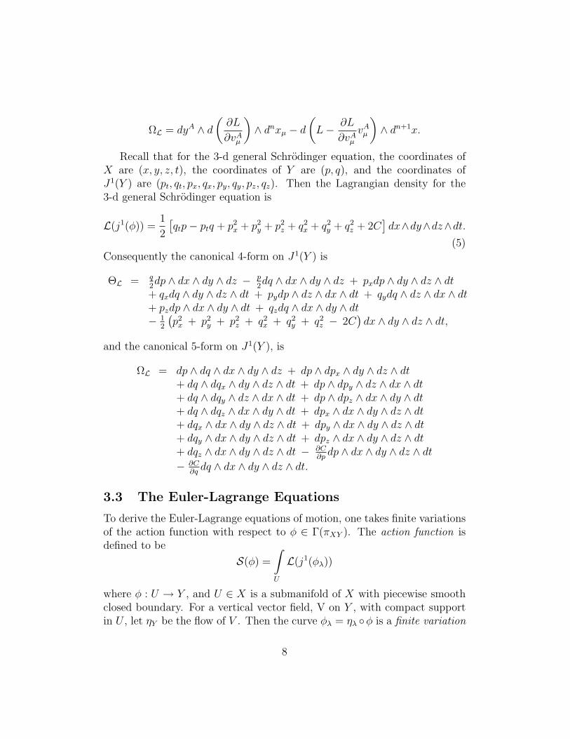
)∧ dn+1x.

Recall that for the 3-d general Schrodinger equation, the coordinates ofX are (x, y, z, t), the coordinates of Y are (p, q), and the coordinates ofJ1(Y ) are (pt, qt, px, qx, py, qy, pz, qz). Then the Lagrangian density for the3-d general Schrodinger equation is

L(j1(φ)) =1

2

[qtp− ptq + p2

x + p2y + p2

z + q2x + q2

y + q2z + 2C

]dx∧dy∧dz∧dt.

(5)Consequently the canonical 4-form on J1(Y ) is

ΘL = q2dp ∧ dx ∧ dy ∧ dz − p

2dq ∧ dx ∧ dy ∧ dz + pxdp ∧ dy ∧ dz ∧ dt

+ qxdq ∧ dy ∧ dz ∧ dt + pydp ∧ dz ∧ dx ∧ dt + qydq ∧ dz ∧ dx ∧ dt+ pzdp ∧ dx ∧ dy ∧ dt + qzdq ∧ dx ∧ dy ∧ dt− 1

2

(p2

x + p2y + p2

z + q2x + q2

y + q2z − 2C

)dx ∧ dy ∧ dz ∧ dt,

and the canonical 5-form on J1(Y ), is

ΩL = dp ∧ dq ∧ dx ∧ dy ∧ dz + dp ∧ dpx ∧ dy ∧ dz ∧ dt+ dq ∧ dqx ∧ dy ∧ dz ∧ dt + dp ∧ dpy ∧ dz ∧ dx ∧ dt+ dq ∧ dqy ∧ dz ∧ dx ∧ dt + dp ∧ dpz ∧ dx ∧ dy ∧ dt+ dq ∧ dqz ∧ dx ∧ dy ∧ dt + dpx ∧ dx ∧ dy ∧ dz ∧ dt+ dqx ∧ dx ∧ dy ∧ dz ∧ dt + dpy ∧ dx ∧ dy ∧ dz ∧ dt+ dqy ∧ dx ∧ dy ∧ dz ∧ dt + dpz ∧ dx ∧ dy ∧ dz ∧ dt+ dqz ∧ dx ∧ dy ∧ dz ∧ dt − ∂C

∂pdp ∧ dx ∧ dy ∧ dz ∧ dt

− ∂C∂q

dq ∧ dx ∧ dy ∧ dz ∧ dt.

3.3 The Euler-Lagrange Equations

To derive the Euler-Lagrange equations of motion, one takes finite variationsof the action function with respect to φ ∈ Γ(πXY ). The action function isdefined to be

S(φ) =

∫U

L(j1(φλ))

where φ : U → Y , and U ∈ X is a submanifold of X with piecewise smoothclosed boundary. For a vertical vector field, V on Y , with compact supportin U , let ηY be the flow of V . Then the curve φλ = ηλ φ is a finite variation

8

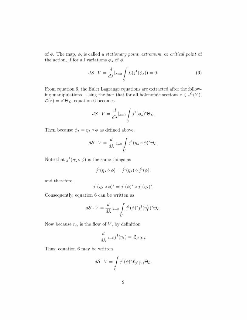
of φ. The map, φ, is called a stationary point, extremum, or critical point ofthe action, if for all variations φλ of φ,

dS · V =d

dλ|λ=0

∫U

L(j1(φλ)) = 0. (6)

From equation 6, the Euler Lagrange equations are extracted after the follow-ing manipulations. Using the fact that for all holonomic sections z ∈ J1(Y ),L(z) = z∗ΘL, equation 6 becomes

dS · V =d

dλ|λ=0

∫U

j1(φλ)∗ΘL.

Then because φλ = ηλ φ as defined above,

dS · V =d

dλ|λ=0

∫U

j1(ηλ φ)∗ΘL.

Note that j1(ηλ φ) is the same things as

j1(ηλ φ) = j1(ηλ) j1(φ),

and therefore,j1(ηλ φ)∗ = j1(φ)∗ j1(ηλ)

∗.

Consequently, equation 6 can be written as

dS · V =d

dλ|λ=0

∫U

j1(φ)∗j1(ηλY )∗ΘL.

Now because nλ is the flow of V , by definition

d

dλ|λ=0j

1(ηλ) = Lj1(V ).

Thus, equation 6 may be written

dS · V =

∫U

j1(φ)∗Lj1(V )ΘL.

9

Recall that Cartan’s magic formula says Lj1(V )ΘL = ij1(V )dΘL + d ij1(V )ΘL.Also, by definition, dΘL = −ΩL. Accordingly, equation 6 becomes

dS · V =∫U

j1(φ)∗(ij1(V )dΘL + d ij1(V )ΘL

)=

∫U

j1(φ)∗(ij1(V )ΩL + d ij1(V )ΘL

)=

∫U

j1(φ)∗ij1(V )ΩL +∫U

j1(φ)∗d ij1(V )ΘL.

Employing Stokes theorem

dS · V =

∫U

j1(φ)∗ij1(V )ΩL +

∫∂U

j1(φ)∗ij1(V )ΘL. (7)

In order for φ to an extremum of S, both terms in 7 must disappear. Themultisymplectic form formula, (stated later), employs in its proof the secondterm of 7, which is ∫

∂U

j1(φ)∗ij1(V )ΘL = 0.

This is to be discussed later. However, the first term in equation 7,∫U

j1(φ)∗ij1(V )ΩL = 0,

is to be discussed here, because it is from this term that the Euler Lagrangeequations are extracted. The above condition is true, whenever j1(V ) =W ∈ TJ1(Y ), where TJ1(Y ) consists of vector fields on J1(Y ) that areπY,J1(Y ) vertical, or tangent to j1(φ). Thus, φ is said to be a solution to theEuler-Lagrange equations whenever

j1(φ)∗iW ΩL = 0 (8)

for some W ∈ TJ1(Y ). This very expression, in equation 8, written incoordinates, is the set of Euler-Lagrange equations

∂L

∂yA(j1(φ))− ∂

∂xµ

(∂L

∂vAµ

(j1(φ))

)= 0.

Note that as mentioned before, xµ are coordinates of the base manifoldX, yA are coordinates Y , which is the fiber bundle over X, and vA

µ arecoordinates of J1(Y ), which is the first jet bundle over Y .

10

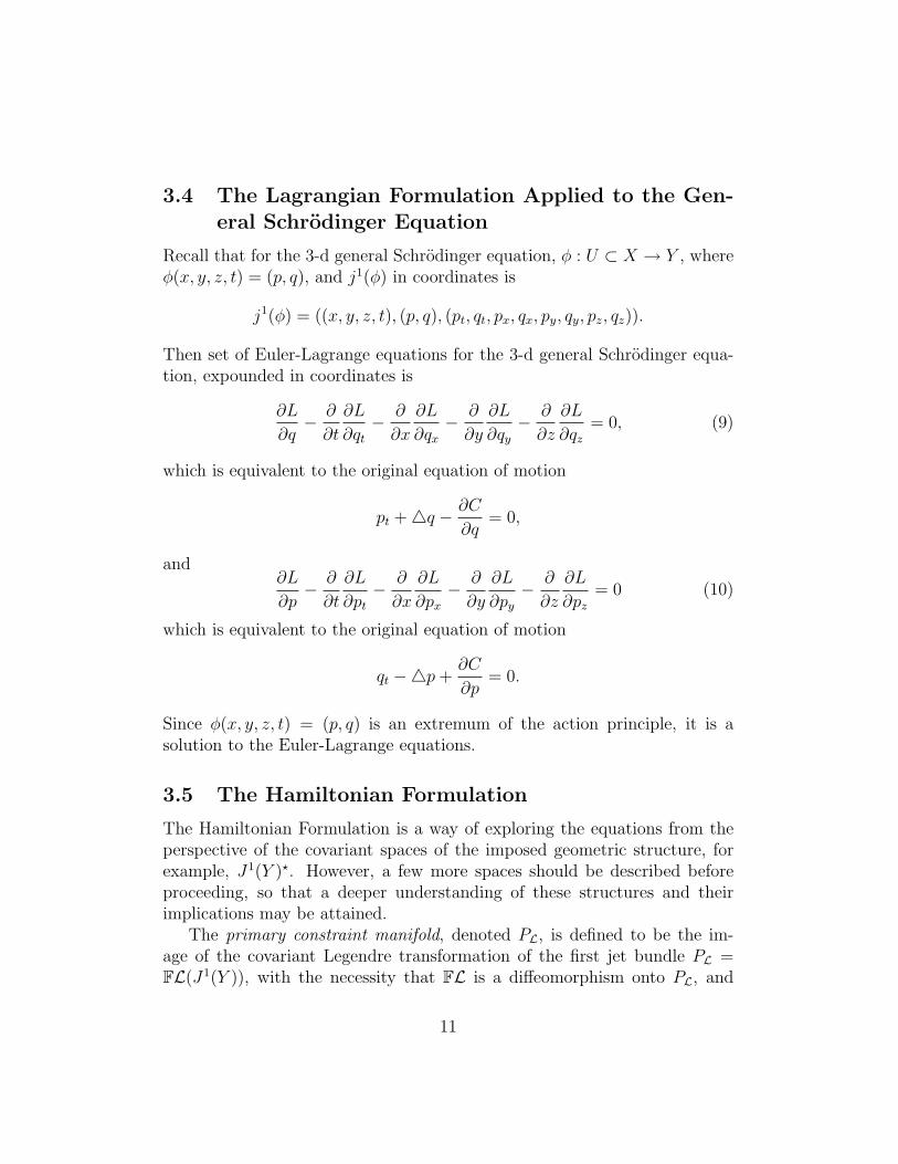
3.4 The Lagrangian Formulation Applied to the Gen-eral Schrodinger Equation

Recall that for the 3-d general Schrodinger equation, φ : U ⊂ X → Y , whereφ(x, y, z, t) = (p, q), and j1(φ) in coordinates is

j1(φ) = ((x, y, z, t), (p, q), (pt, qt, px, qx, py, qy, pz, qz)).

Then set of Euler-Lagrange equations for the 3-d general Schrodinger equa-tion, expounded in coordinates is

∂L

∂q− ∂

∂t

∂L

∂qt

− ∂

∂x

∂L

∂qx

− ∂

∂y

∂L

∂qy

− ∂

∂z

∂L

∂qz

= 0, (9)

which is equivalent to the original equation of motion

pt +4q − ∂C

∂q= 0,

and∂L

∂p− ∂

∂t

∂L

∂pt

− ∂

∂x

∂L

∂px

− ∂

∂y

∂L

∂py

− ∂

∂z

∂L

∂pz

= 0 (10)

which is equivalent to the original equation of motion

qt −4p +∂C

∂p= 0.

Since φ(x, y, z, t) = (p, q) is an extremum of the action principle, it is asolution to the Euler-Lagrange equations.

3.5 The Hamiltonian Formulation

The Hamiltonian Formulation is a way of exploring the equations from theperspective of the covariant spaces of the imposed geometric structure, forexample, J1(Y )?. However, a few more spaces should be described beforeproceeding, so that a deeper understanding of these structures and theirimplications may be attained.

The primary constraint manifold, denoted PL, is defined to be the im-age of the covariant Legendre transformation of the first jet bundle PL =FL(J1(Y )), with the necessity that FL is a diffeomorphism onto PL, and

11

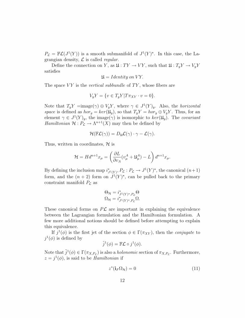
PL = FL(J1(Y )) is a smooth submanifold of J1(Y )?. In this case, the La-grangian density, L is called regular.

Define the connection on Y , as U : TY → V Y , such that U : TyY → VyYsatisfies

U = Identity on V Y.

The space V Y is the vertical subbundle of TY , whose fibers are

VyY = v ∈ TyY |TπXY · v = 0.

Note that TyY =image(γ) ⊕ VyY , where γ ∈ J1(Y )y. Also, the horizontalspace is defined as hory = ker(Uy), so that TyY = hory ⊕ VyY . Thus, for anelement γ ∈ J1(Y )y, the image(γ) is isomorphic to ker(Uy). The covariantHamiltonian H : PL → Λn+1(X) may then be defined by

H(FL(γ)) = DUL(γ) · γ − L(γ).

Thus, written in coordinates, H is

H = Hdn+1xµ =

(∂L

∂vA

(vAµ + UA

µ )− L

)dn+1xµ.

By defining the inclusion map i∗J1(Y ), PL : PL → J1(Y )?, the canonical (n+1)

form, and the (n + 2) form on J1(Y )?, can be pulled back to the primaryconstraint manifold PL as

ΘH = i∗J1(Y )?,PLΘ

ΩH = i∗J1(Y )?,PLΩ.

These canonical forms on PL are important in explaining the equivalencebetween the Lagrangian formulation and the Hamiltonian formulation. Afew more additional notions should be defined before attempting to explainthis equivalence.

If j1(φ) is the first jet of the section φ ∈ Γ(πXY ), then the conjugate toj1(φ) is defined by

j1(φ) = FL j1(φ).

Note that j1(φ) ∈ Γ(πX,PL) is also a holonomic section of πX,PL . Furthermore,z = j1(φ), is said to be Hamiltonian if

z∗(iF ΩH) = 0 (11)

12

for all F ∈ T (PL). Equation 11 is the set of multihamiltonian equations. Theset of multihamiltonian equations and the set of Euler-Lagrange equationsare said to be implicative of each other. This implication is stated in thefollowing Lemma that was extracted from Marsden, and Shkoller 1.

Lemma 1. If FL : J1(Y ) → PL is a fiber bundle diffeomorphism over Y ,and φ ∈ Γ(πXY ), then the following are equivalent

(i) j1(φ)∗iUΩH = 0, ∀U ∈ T (PL);(ii) j1(φ)∗iW ΩL = 0, ∀W ∈ T (J1(Y )).

Note that (i) is the set of multihamiltonian equations, and (ii) is the set ofEuler-Lagrange equations.

The proof of Lemma 1 can be found in Marsden, and Shkoller 1. Thefollowing theorem was also extracted from Marsden, and Shkoller 1, explainsthe equivalence of the solution of the Euler-Lagrange equations to the solutionof multihamiltonian equations.

Theorem 1. If FL : J1(Y ) → PL is a fiber bundle diffeomorphism over Y ,and φ ∈ ΓπXY , then the following are equivalent:

(i) φ is a stationary point of∫

XL(j1(φ));

(ii) j1(φ) is a Hamiltonian section for H.

Note that φ is a solution to the Euler-Lagrange equations, and j1(φ) solves theset of multihamiltonian equations. Thus, solving the Euler-Lagrange equa-tions is equivalent to solving the multihamiltonian equations.

The following proposition is also taken from Marsden, and Shkoller 1.

Proposition 1. If FL : J1(Y ) → PL is a fiber diffeomorphism and φ ∈Γ(πXY , then j1(φ) is a Hamiltonian system for H if and only if

i ∂∂xµ

j1(φ)(dfµ ∧ dφ) = −dH(j1(φ)). (12)

where µ ∈ 1, . . . , (n + 1).It is noteworthy that 12 is equivalent to the equation in Bridges3.

Mµ ∂n

∂xµ= −∇nH(n),

where the index µ denotes a sum over all coordinates in the base space, andn is the vector n = (yA, vA

ν ), where ν denotes the νth spatial coordinate inthe base space. If the dimension of n is (m× 1), then each Mµ is a m×mmatrix, Mµ ∈ Rm×m.

13

3.6 The Hamiltonian Formulation Applied to SchodingerEquation

Recall that the Hamiltonian density of the 3-d general Schrodinger equation,written in coordinates, is

H = Hdn+1xµ =

(∂L

∂vA

(vAµ + UA

µ )− L

)dn+1xµ.

Thus, a connection, U, must be employed before proceeding. In this case, thetrivial connection is selected. The trivial connection is merely the naturalprojection, where the action is coordinated by (0, vA), and thus, UA

µ = 0.Consequently, the covariant Hamiltonian for the 3-d general Schrodingerequation is regarded as H = Hdx ∧ dy ∧ dz ∧ dt, where

H =∂L

∂pt

pt +∂L

∂qt

qt +∂L

∂px

px +∂L

∂qx

qx +∂L

∂py

py +∂L

∂qy

qy +∂L

∂pz

pz +∂L

∂qz

qz − L

and thusly,

H =1

2

(p2

x + p2y + p2

z + q2x + q2

y + q2z − 2C

). (13)

To case the equations of motion in a hamiltonian formulation, the followingchange of coordinates is utilized

v1 = ∂L∂px

= px w1 = ∂L∂qx

= qx

v2 = ∂L∂py

= py w2 = ∂L∂qy

= qy

v3 = ∂L∂pz

= pz w3 = ∂L∂qz

= qz.

Recasting equation 3 using these coordinates yields the first order equations

qt − v1x − v2y − v3y = −∂C∂p

−pt − w1x − w2y − w3y = −∂C∂q

px = v1

qx = w1

py = v2

qy = w2

pz = v3

qz = w3.

(14)

14

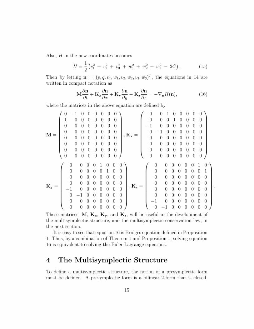
Also, H in the new coordinates becomes

H =1

2

(v2

1 + v22 + v2

3 + w21 + w2

2 + w23 − 2C

). (15)

Then by letting n = (p, q, v1, w1, v2, w2, v3, w3)T , the equations in 14 are

written in compact notation as

M∂n

∂t+ Kx

∂n

∂x+ Ky

∂n

∂y+ Kz

∂n

∂z= −∇nH(n), (16)

where the matrices in the above equation are defined by

M =

0 −1 0 0 0 0 0 01 0 0 0 0 0 0 00 0 0 0 0 0 0 00 0 0 0 0 0 0 00 0 0 0 0 0 0 00 0 0 0 0 0 0 00 0 0 0 0 0 0 00 0 0 0 0 0 0 0

,Kx =

0 0 1 0 0 0 0 00 0 0 1 0 0 0 0

−1 0 0 0 0 0 0 00 −1 0 0 0 0 0 00 0 0 0 0 0 0 00 0 0 0 0 0 0 00 0 0 0 0 0 0 00 0 0 0 0 0 0 0

Ky =

0 0 0 0 1 0 0 00 0 0 0 0 1 0 00 0 0 0 0 0 0 00 0 0 0 0 0 0 0

−1 0 0 0 0 0 0 00 −1 0 0 0 0 0 00 0 0 0 0 0 0 00 0 0 0 0 0 0 0

,Kz =

0 0 0 0 0 0 1 00 0 0 0 0 0 0 10 0 0 0 0 0 0 00 0 0 0 0 0 0 00 0 0 0 0 0 0 00 0 0 0 0 0 0 0

−1 0 0 0 0 0 0 00 −1 0 0 0 0 0 0

.

These matrices, M, Kx, Ky, and Kz, will be useful in the development ofthe multisymplectic structure, and the multisymplectic conservation law, inthe next section.

It is easy to see that equation 16 is Bridges equation defined in Proposition1. Thus, by a combination of Theorem 1 and Proposition 1, solving equation16 is equivalent to solving the Euler-Lagrange equations.

4 The Multisymplectic Structure

To define a multisymplectic structure, the notion of a presymplectic formmust be defined. A presymplectic form is a bilinear 2-form that is closed,

15

skew-symmetric, but not necessarily nondegenerate. A set of presymplecticforms together with a manifold comprise a multisymplectic structure. For thematrices M, Kx, Ky, and Kz, in the previous section, define the presym-plectic forms:

ω(a, b) = 〈Ma, b〉κx(a, b) = 〈Kxa, b〉κy(a, b) = 〈Kya, b〉κz(a, b) = 〈Kza, b〉

where the matrix representation of these forms is defined by

g(a, b) = 〈Ga, b〉 = aT GT b,

where G ∈ R8×8. Then (TJ1(Y ), ω, κx, κy, κz) is a multisymplectic structureof the general Schrodinger equation.

5 The Multisymplectic Form Formula

Before stating the multisymplectic form formula, it is necessary to classifythe types of sections and vector fields that are employed in theorem, so thatit will hold true.

Suppose U ⊂ X is a smooth submanifold, with piecewise smooth closedboundary. Then C∞ is the set of smooth maps

C∞ = φ : U → Y |πXY φ : U → X is an embedding.

Define C as the infinite dimensional manifold that is the closure of C∞ inthe Hilbert space. Next, define the set of solutions to the Euler-Lagrangeequations

P = φ ∈ C|j1(φ)∗iW ΩL = 0, ∀W ∈ TJ1(Y ).

Lastly, define the set of vector fields that solve the first variation equation tothe Euler-Lagrange equations (in equation 6)

F = V ∈ TφC|j1(φ)∗Lj1(V )iBΩL = 0, ∀B ∈ TJ1(Y ).

Now that all of the necessary components have been stated, the multisym-plectic form formula may be introduced.

16

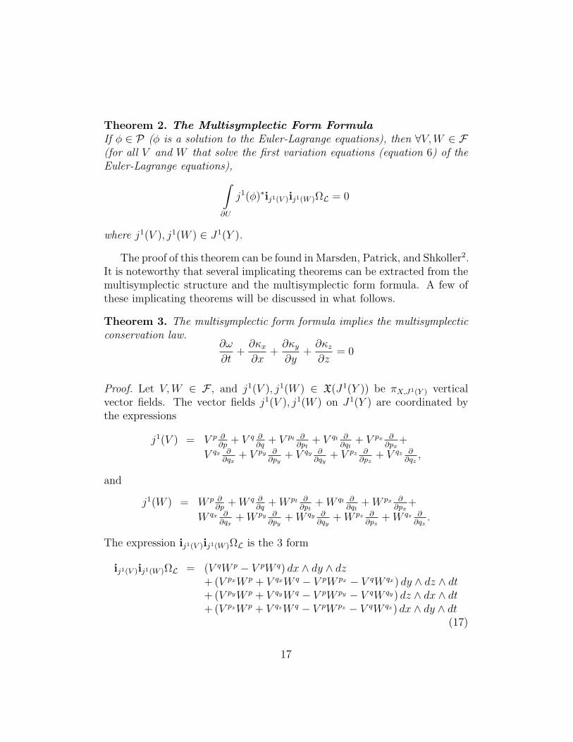
Theorem 2. The Multisymplectic Form FormulaIf φ ∈ P (φ is a solution to the Euler-Lagrange equations), then ∀V, W ∈ F(for all V and W that solve the first variation equations (equation 6) of theEuler-Lagrange equations),∫

∂U

j1(φ)∗ij1(V )ij1(W )ΩL = 0

where j1(V ), j1(W ) ∈ J1(Y ).

The proof of this theorem can be found in Marsden, Patrick, and Shkoller2.It is noteworthy that several implicating theorems can be extracted from themultisymplectic structure and the multisymplectic form formula. A few ofthese implicating theorems will be discussed in what follows.

Theorem 3. The multisymplectic form formula implies the multisymplecticconservation law.

∂ω

∂t+

∂κx

∂x+

∂κy

∂y+

∂κz

∂z= 0

Proof. Let V, W ∈ F , and j1(V ), j1(W ) ∈ X(J1(Y )) be πX,J1(Y ) verticalvector fields. The vector fields j1(V ), j1(W ) on J1(Y ) are coordinated bythe expressions

j1(V ) = V p ∂∂p

+ V q ∂∂q

+ V pt ∂∂pt

+ V qt ∂∂qt

+ V px ∂∂px

+

V qx ∂∂qx

+ V py ∂∂py

+ V qy ∂∂qy

+ V pz ∂∂pz

+ V qz ∂∂qz

,

and

j1(W ) = W p ∂∂p

+ W q ∂∂q

+ W pt ∂∂pt

+ W qt ∂∂qt

+ W px ∂∂px

+

W qx ∂∂qx

+ W py ∂∂py

+ W qy ∂∂qy

+ W pz ∂∂pz

+ W qz ∂∂qz

.

The expression ij1(V )ij1(W )ΩL is the 3 form

ij1(V )ij1(W )ΩL = (V qW p − V pW q) dx ∧ dy ∧ dz+ (V pxW p + V qxW q − V pW px − V qW qx) dy ∧ dz ∧ dt+ (V pyW p + V qyW q − V pW py − V qW qy) dz ∧ dx ∧ dt+ (V pzW p + V qzW q − V pW pz − V qW qz) dx ∧ dy ∧ dt

(17)

17

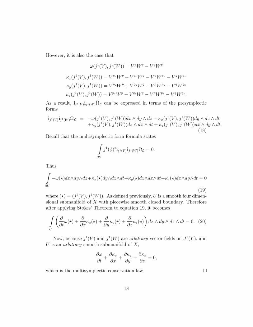
However, it is also the case that

ω(j1(V ), j1(W )) = V pW q − V qW p

κx(j1(V ), j1(W )) = V pxW p + V qxW q − V pW px − V qW qx

κy(j1(V ), j1(W )) = V pyW p + V qyW q − V pW py − V qW qy

κz(j1(V ), j1(W )) = V pzW p + V qzW q − V pW pz − V qW qz .

As a result, ij1(V )ij1(W )ΩL can be expressed in terms of the presymplecticforms

ij1(V )ij1(W )ΩL = −ω(j1(V ), j1(W ))dx ∧ dy ∧ dz + κx(j1(V ), j1(W ))dy ∧ dz ∧ dt

+κy(j1(V ), j1(W ))dz ∧ dx ∧ dt + κz(j

1(V ), j1(W ))dx ∧ dy ∧ dt.(18)

Recall that the multisymplectic form formula states∫∂U

j1(φ)∗ij1(V )ij1(W )ΩL = 0.

Thus∫∂U

−ω(?)dx∧dy∧dz+κx(?)dy∧dz∧dt+κy(?)dz∧dx∧dt+κz(?)dx∧dy∧dt = 0

(19)where (?) = (j1(V ), j1(W )). As defined previously, U is a smooth four dimen-sional submanifold of X with piecewise smooth closed boundary. Thereforeafter applying Stokes’ Theorem to equation 19, it becomes∫

U

(∂

∂tω(?) +

∂

∂xκx(?) +

∂

∂yκy(?) +

∂

∂zκz(?)

)dx ∧ dy ∧ dz ∧ dt = 0. (20)

Now, because j1(V ) and j1(W ) are arbitrary vector fields on J1(Y ), andU is an arbitrary smooth submanifold of X,

∂ω

∂t+

∂κx

∂x+

∂κy

∂y+

∂κz

∂z= 0,

which is the multisymplectic conservation law.

18

Theorem 4. For the case where the base space U ⊂ X is coordinated withinfinite spatial domain, in other words, if

U = (x, y, z, t) ∈ R3 × R | x ∈ (−∞,∞), y ∈ (−∞,∞), & z ∈ (−∞,∞),

then the relationship between the quantum mechanical symplectic form, Ω(Ψ, Φ),and the presymplectic form, ω (j1(V ), j1(W )), is

Ω(Ψ, Φ) = −2

∫∂U

ω(j1(V ), j1(W )

)dx ∧ dy ∧ dz.

Please note that in this case, j1(V ) is associated with the wavefunction Ψ,and j1(W ) is associated with the wavefunction Φ, in the following manner

j1(V ) = pΨ ∂∂p

+ qΨ ∂∂q

+ V pt ∂∂pt

+ V qt ∂∂qt

+ V px ∂∂px

+

V qx ∂∂qx

+ V py ∂∂py

+ V qy ∂∂qy

+ V pz ∂∂pz

+ V qz ∂∂qz

and

j1(W ) = pΦ ∂∂p

+ qΦ ∂∂q

+ W pt ∂∂pt

+ W qt ∂∂qt

+ W px ∂∂px

+

W qx ∂∂qx

+ W py ∂∂py

+ W qy ∂∂qy

+ W pz ∂∂pz

+ W qz ∂∂qz

.

where pΨ = ReΨ, qΨ = ImΨ, and pΦ = ReΦ, qΨ = ImΦ.

Note that the quantum mechanical symplectic form is defined in terms ofthe ordinary quantum mechancial Hermitian inner product on the complexHilbert space of L2 wavefunctions 4, 〈〈Ψ, Φ〉〉, as

Ω(Ψ, Φ) = −2Im〈〈Ψ, Φ〉〉.

Proof. The presymplectic form, ω(·, ·), acting on the vector fields, j1(V ), j1(W ) ∈TJ1(Y ), as defined above, is

ω(j1(V ), j1(W )

)= pΨqΦ − qΨpΦ.

Thus∫∂U

ω(j1(V ), j1(W )

)dx ∧ dy ∧ dz =

∫∂U

(pΨqΦ − qΨpΦ

)dx ∧ dy ∧ dz. (21)

19

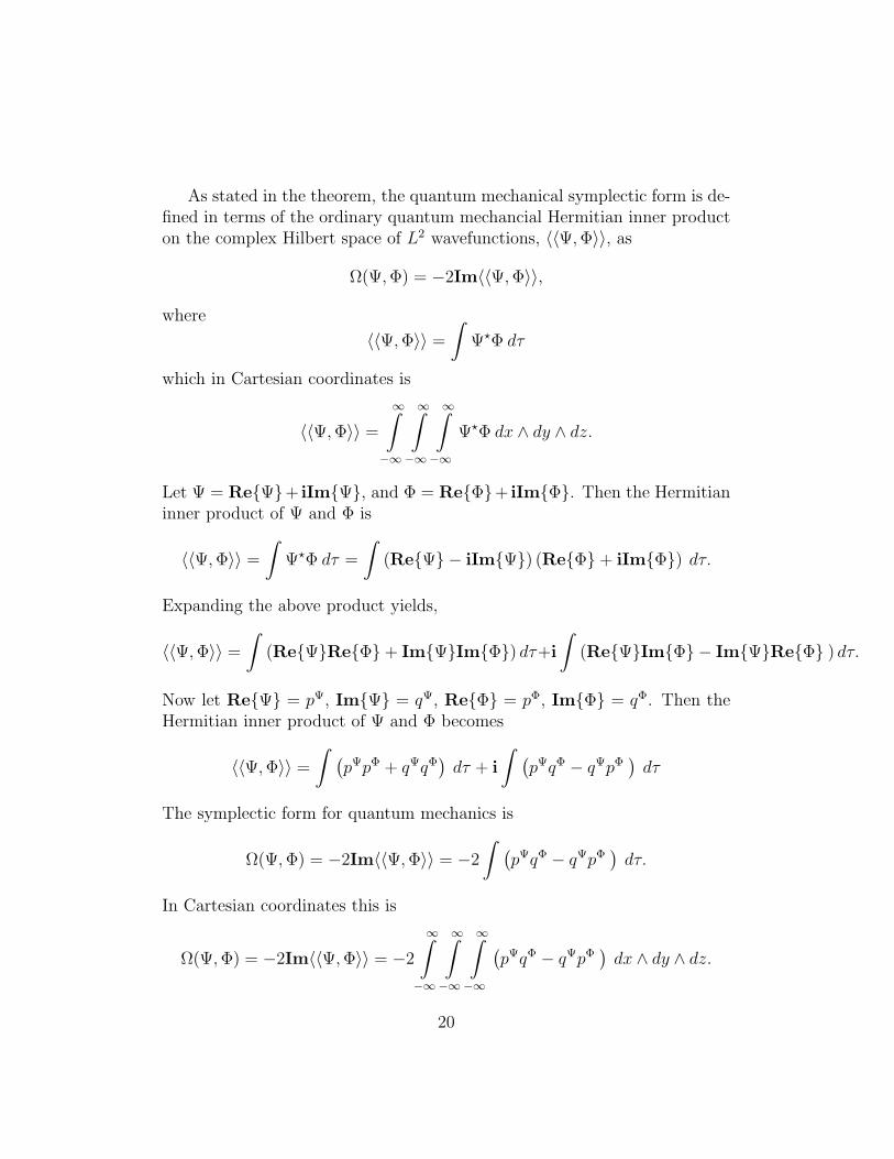
As stated in the theorem, the quantum mechanical symplectic form is de-fined in terms of the ordinary quantum mechancial Hermitian inner producton the complex Hilbert space of L2 wavefunctions, 〈〈Ψ, Φ〉〉, as

Ω(Ψ, Φ) = −2Im〈〈Ψ, Φ〉〉,

where

〈〈Ψ, Φ〉〉 =

∫Ψ?Φ dτ

which in Cartesian coordinates is

〈〈Ψ, Φ〉〉 =

∞∫−∞

∞∫−∞

∞∫−∞

Ψ?Φ dx ∧ dy ∧ dz.

Let Ψ = ReΨ+ iImΨ, and Φ = ReΦ+ iImΦ. Then the Hermitianinner product of Ψ and Φ is

〈〈Ψ, Φ〉〉 =

∫Ψ?Φ dτ =

∫(ReΨ − iImΨ) (ReΦ+ iImΦ) dτ.

Expanding the above product yields,

〈〈Ψ, Φ〉〉 =

∫(ReΨReΦ+ ImΨImΦ) dτ+i

∫(ReΨImΦ − ImΨReΦ ) dτ.

Now let ReΨ = pΨ, ImΨ = qΨ, ReΦ = pΦ, ImΦ = qΦ. Then theHermitian inner product of Ψ and Φ becomes

〈〈Ψ, Φ〉〉 =

∫ (pΨpΦ + qΨqΦ

)dτ + i

∫ (pΨqΦ − qΨpΦ

)dτ

The symplectic form for quantum mechanics is

Ω(Ψ, Φ) = −2Im〈〈Ψ, Φ〉〉 = −2

∫ (pΨqΦ − qΨpΦ

)dτ.

In Cartesian coordinates this is

Ω(Ψ, Φ) = −2Im〈〈Ψ, Φ〉〉 = −2

∞∫−∞

∞∫−∞

∞∫−∞

(pΨqΦ − qΨpΦ

)dx ∧ dy ∧ dz.

20

But because

U = (x, y, z, t) ∈ R3 × R | x ∈ (−∞,∞), y ∈ (−∞,∞), & z ∈ (−∞,∞),

then∫∂U

ω(j1(V ), j1(W )

)dx∧dy∧dz =

∞∫−∞

∞∫−∞

∞∫−∞

ω(j1(V ), j1(W )

)dx∧dy∧dz = Im〈〈Ψ, Φ〉〉.

and consequently

Ω(Ψ, Φ) = −2

∞∫−∞

∞∫−∞

∞∫−∞

ω(j1(V ), j1(W )

)dx ∧ dy ∧ dz.

Therefore, it is proven that:

Ω(Ψ, Φ) = −2

∫∂U

ω(j1(V ), j1(W )

)dx ∧ dy ∧ dz.

Theorem 5. For the 3-d general Schrodinger equation with infinite spatialdomain, and bounded time domain, t ∈ [T1, T2], the integrals along the bound-aries at t = T1 and t = T2 are equal in magnitude but opposite in orientation.In other words∫

∂UT1

ω(j1(V ), j1(W ))dx ∧ dy ∧ dz = −∫

∂UT2

ω(j1(V ), j1(W ))dx ∧ dy ∧ dz.

Proof. From the proof of 5, the multisymplectic form formula implies that∫∂U

−ω(?)dx∧dy∧dz+κx(?)dy∧dz∧dt+κy(?)dz∧dx∧dt+κz(?)dx∧dy∧dt = 0.

(22)Now, for reasons explained after the following statement, the multisymplecticform formula applied to a system with an infinite spatial domain but boundedtime domain reduces to∫

∂U

ω(j1(V ), j1(W ))dx ∧ dy ∧ dz = 0. (23)

21

This phenomena occurs due to the fact that in the multisymplectic formformula, the integration takes place along the boundary of the domain U . Yet,for the case that the system possesses bounded time domain, and unbounded,or infinite spatial domain, there does not exist a boundary that proceeds alongthe temporal domain, upon which to integrate. Thus, each form in 22 thatincludes the term dt, simply disappears.

Now because the time coordinate is bounded, this means that there is anupper limit in time, and a lower limit in time. Thus, for each integration inthe triple integral, there are two boundaries to integrate along in equation23. Denote the lower boundary by ∂UT1 , and the upper boundary by ∂UT2 .Then equation 23 becomes∫∂UT1

ω(j1(V ), j1(W ))dx ∧ dy ∧ dz +

∫∂UT2

ω(j1(V ), j1(W ))dx ∧ dy ∧ dz = 0.

As a result,∫∂UT1

ω(j1(V ), j1(W ))dx ∧ dy ∧ dz = −∫

∂UT2

ω(j1(V ), j1(W ))dx ∧ dy ∧ dz.

Thus, the integrals along the boundaries at time t = T1 and time t = T2, thatis, the integrals along ∂UT1 and ∂UT2 , are equal in magnitude, but oppositein orientation.

22

6 Conclusion

The methodology in this paper can certainly be easily extended to higherdimensional systems. For example, for a system with N particles, the 3N -dimensional Schrodinger equation can be geometrized in an analogous fash-ion, with the base space being coordinated by 3N spatial coordinates insteadof 3. Additionally, the base space may be coordinated by any other depen-dent variable that one may wish to consider, that the wavefunction is relatedto.

The geometric framework presented in this paper can be utilized to de-rive integrators for various partial differential equations. For example, theVeselov-type discretization, normally applied to the regular Lagrangian for-mulation, may be applied to multisymplectic field theory for the purpose ofderiving variational integrators1. This method was applied in Chen5 to thenonlinear Schrodinger equation. It is hoped that the work presented here haslaid the groundwork for Veselov-type discretization techniques to be appliedto the general Schrodinger equation.

Optimistically, the geometric structure imposed on the Schrodinger equa-tion will lead to greater insight in one’s study of theoretical physics andchemistry. The trick is to relate the mathematical objects in this frameworkto an object or idea that corresponds to reality in the physical world. Forexample, what does the multisymplectic conservation law correspond to inthe ”real world”? Most likely this idea has already been explored. However,asking such types of question will lead to either 1) a higher level of knowledgethat is already known, 2) a higher level of discovery in quantum mechanics,or 3) a wider area of application. All three areas are well worth the effortthat will take to pose and answer such questions.

23

7 References

1. J.E. Marsden, S. Shkoller, Math. Proc. Camb. Phil. Soc., 125, 553-575, (1999).

2. J.E. Marsden, G.W. Patrick, S. Shkoller, Comm. Math. Phys., 199,351-395, (1998).

3. T.J. Bridges, Math. Proc. Phil. Soc., 121, 147-190, (1997).

4. J.E. Marsden, T.S. Ratiu, Introduction to Mechanics and Symmetry,Springer-Verlag, (1999).

5. J.B. Chen, M.Z. Qin, Numer. Math. Partial Differential Equations,18, 523-536, (2002).

24