Electronic copy available at: http://ssrn.com/abstract=2631929

Multitasking, Multi-Armed Bandits, and the Italian Judiciary∗

Robert L. Bray1, Decio Coviello2, Andrea Ichino3, and Nicola Persico1

1Kellogg School of Management, Northwestern University

2HEC Montreal

3European University Institute and University of Bologna

March 23, 2016

Abstract

We model how a judge schedules cases as a multi-armed bandit problem. The model indicates

that a first-in-first-out (FIFO) scheduling policy is optimal when the case completion hazard

rate function is monotonic. But there are two ways to implement FIFO in this context: at

the hearing level or at the case level. Our model indicates that the former policy, prioritizing

the oldest hearing, is optimal when the case completion hazard rate function decreases, and

the latter policy, prioritizing the oldest case, is optimal when the case completion hazard rate

function increases. This result convinced six judges of the Roman Labor Court of Appeals—a

court that exhibits increasing hazard rates—to switch from hearing-level FIFO to case-level

FIFO. Tracking these judges for eight years, we estimate that our intervention decreased the

average case duration by 12% and the probability of a decision being appealed to the Italian

supreme court by 3.8%, relative to a 44-judge control sample.

Keywords: multitasking; multi-armed bandits; field experiment; Italian judiciary; production

scheduling

∗We thank Antonio Moreno and Thomas Bray for their helpful suggestions.

1

Electronic copy available at: http://ssrn.com/abstract=2631929

1 Introduction

The Italian judiciary is slow. The World Bank ranks Italy 147th out of 189 countries in ease

of enforcing contracts: It takes an estimated 3.25 years to enforce a contract in Italy, slightly

less than Djibouti (3.35), and slightly more than Myanmar (3.18) (World Bank Group, 2014).

Among developed countries, Italy is a judicial outlier—twice as slow as any other member of the

Organization for Economic Co-operation and Development (OECD), a trade confederation of 34

industrialized countries (OECD, 2013). And the problem is getting worse; the stock of pending

civil cases increased by 10% from 2008 to 2010 (Esposito et al., 2014, p. 6), and the average Italian

civil case duration increased by 19% from 2010 to 2012 (CEPEJ, 2014b, p. 200). The International

Monetary Fund (IMF) argues that the inefficiency of Italian courts leads to “reduced investments,

slow growth, and a difficult business environment” (Esposito et al., 2014, p. 1).

We study the Italian Labor Court of Appeals. Italy’s appellate courts are especially sluggish:

The average Italian case is 2.4 times as long as the average OECD case at the trial level, and

4.7 times as long at the appellate level (OECD, 2013). And Italy’s labor courts are vital, as the

IMF explains: “[Italy’s] inefficient labor courts can have detrimental effects on the composition

of employment and labor market participation. [They] also affect job reallocation, which in turn

impacts productivity and capital intensity” (Esposito et al., 2014, p. 5).

Several top-down initiatives have failed to reform the Italian judiciary. The European Commis-

sion for the Efficiency of Justice (CEPEJ) recommended “good practices and innovative suggestions”

(CEPEJ, 2006), but the Italian judiciary ignored these. The Parliament passed a law that reduced

judge summer vacations from 45 to 30 days, but the judiciary refused to apply it (Chirico, 2013;

ANSA, 2015). And the Italian judiciary’s self-governing body appointed a special commission to

develop productivity benchmarks, but the judges on the panel failed to find consensus (Unita’ per

la Costituzione, 2015).

Italian judges could resist these top-down reforms because they are politically independent

2

and operate with little oversight. Accordingly, bottom-up reforms, shepherded by judges, have

more potential for efficacy. To galvanize judicial action, a policy should (i) be clearly beneficial,

(ii) preserve judicial autonomy, (iii) not increase workloads, and (iv) be easy to understand and

implement. We identify such a policy improvement in the Roman Labor Court of Appeals.

This court’s cases generally require two or three hearings. Traditionally, the judges scheduled

one at a time, arranging a case’s (n + 1)th hearing during its nth hearing. Consequently, every

hearing joined the end of a judge’s work queue (when his or her calendar was next free); thus, cases

comprising N hearings would cycle through the work queue (the calendar) N times. We call this

policy, which prioritizes the oldest hearing, hearing-level FIFO. We propose a new scheduling policy

in which cases traverse the docket only once: case-level FIFO. Under this policy, a judge selects

the oldest case and works on it to fruition before opening a new case. More accurately, we propose

a relaxation of case-level FIFO, as the policy in its strictest sense violates scheduling constraints.

The judges implement relaxed case-level FIFO by estimating the number of hearings a new case

will require and scheduling that many up front (reserving preparation time between hearings). This

scheduling policy mimics case-level FIFO by minimizing queue re-entry.

Switching from hearing-level FIFO to relaxed case-level FIFO decreases the number of cycles

through the queue, but increases the length of the queue (as multiple hearings per case queue up).

With a multi-armed bandit production scheduling model, we show that the former effect dominates

the latter, for an overall flow time drop, when the likelihood of finishing a case increases with the

hearing number—i.e., when the case completion hazard rate function increases. Intuitively, when

the case completion hazard rate function slopes upwards, judges should prioritize cases they have

already seen because those cases are more likely to reach completion; this is what case-level FIFO

does.

We test this theoretical result empirically with a difference-in-difference research design. First,

we show that the Roman Labor Court of Appeals exhibits increasing case completion hazard rates.

Second, we assign six judges to a treatment group and 44 judges to a control group. Third, we

3

compel the treated judges to adopt the relaxed case-level FIFO policy. And finally, we measure how

the treated judges’ operational performance changes from the five years preceding our intervention

to the three years following, relative to the control sample.

Before our intervention, the treated and control judges completed cases at the same rate; after

our intervention, the treated judges outpaced the control judges by .07 cases a day (11%). By

horizon end, the treated judges decreased their inventories by 87 cases relative to the control

judges, and their case flow times by 111 days (12%). Also, after adopting case-level FIFO, the

treated judges’ rulings were appealed 3.8% less often relative to those of the control judges, which

suggests an improvement in ruling quality.

2 Multitasking Literature Review

Our intervention decreases the degree of judicial multitasking—reducing the number of open cases

that judges need to juggle. The effect of reducing multitasking is complex, and the literature has

identified multiple pros and cons.

2.1 Prioritization by Service Time

This work’s closest antecedents are Coviello et al.’s (2014, 2015) judicial multitasking studies.

Coviello et al. explain that juggling many cases distracts judges from prioritizing cases that require

little remaining service, which leads cases to linger longer in the docket. For example, suppose a

judge has two cases, each requiring two hearings. When the judge finishes the first case before

starting the second, the average case finishes after (2 + 4)/2 = 3 hearings, but when the judge

switches between the cases, the average case finishes after (3 + 4)/2 = 3.5 hearings. Multitasking

increases the average wait by diverting the judge away from the most pressing case—the one about

to finish.

4

Coviello et al. test this theory in the Labor Court of Milan (a court different from ours). They

measure the causal effect of multitasking on case durations with instrumental variables regres-

sions, instrumenting for case juggling with case difficulty. They estimate that increasing judicial

multitasking by 1% increases case flow times by 2%.

We refine Coviello et al.’s analysis. First, we derive the intuition that judges should prioritize

nearly finished cases from a different model; ours frames courthouse scheduling as a stochastic multi-

armed bandit problem, whereas theirs frames it as a deterministic fluid approximation. Second,

whereas Coviello et al. study multitasking passively, exploiting natural variations in preexisting

data, we do so actively, designing a field experiment to isolate its causal effect—whereas they

provide an econometric model that suggests judges could reduce case flow times, we actually reduce

case flow times. This distinction is meaningful, because Coviello et al. never explained whether

the necessary scheduling changes were feasible in the wild. This oversight enabled detractors in the

Italian judicial community to dismiss Coviello et al.’s findings, claiming that it would be impossible

for them to juggle fewer cases. Our field experiment disproves these critics, showing that they can

(i) decrease the degree of multitasking and (ii) decrease flow times in the process.

2.2 Setup Times

Most frame the cost of multitasking in terms of setup times. For example, Wang et al. (2015)

show that physicians at Northwestern Memorial Hospital zigzag between cases, incurring a setup

with each deviation. Wang et al. estimate that if they could eliminate setups, the hospital could

serve 20% more patients. Batt and Terwiesch (2012, p. 7) likewise find “switching costs increase

with increased levels of multitasking” in a hospital: They estimate that increasing the number of

patients from the lower quartile to the upper quartile increases delays by 26%.

We consider a different sort of setup cost: forgetting. It would usually take a judge around

nine months to return to a case, during which time he or she would see upwards of 500 others.

Invariably, the judge would forget the original case, and would thus have to spend much of the

5

follow-up hearing reviewing his or her notes. This is a setup cost. But this differs from a traditional

production setup cost, as the amount forgotten increases with the time the case lies fallow. Our

scheduling policy mitigates judicial forgetting by decreasing the time between hearings from nine

months to six weeks.

2.3 Avoiding Idleness

Aral et al. (2012, p. 851) and Kc (2014, p. 168) likewise document multitasking setup costs.

But they also report a benefit to multitasking: Switching between tasks enables servers to “utilize

lulls in one project to accomplish tasks related to other projects”; indeed, “Switching to a new

task rather than idly waiting on a pending task can thus increase worker utilization and improve

overall productivity.” Accordingly, Aral et al. and Kc recommend a modest level of multitasking to

minimize setup costs while avoiding idleness. Our case scheduling policy indeed specifies a moderate

degree of multitasking. Lawyers need at least six weeks between successive hearings of a case, so

our policy maintains six weeks’ worth of open cases.

2.4 Worker Motivation

Tan and Netessine (2014) and Staats and Gino (2012) document a second reason to multitask:

Switching tasks periodically increases worker morale. Tan and Netessine find that waiters are more

focused when assigned more tables, and Staats and Gino find that bankers are more productive

when assigned work that varies across days.1 Changing the judges’ scheduling policies from hearing-

level to case-level FIFO is unlikely to influence the judges’ motivation because they never see a case

twice in one month under either scheduling policy.

1Tan and Netessine’s and Staats and Gino’s findings could also stem from unrelated workload effects (Kc andTerwiesch, 2009; Powell et al., 2012; Freeman et al., 2015).

6

3 Theoretical Motivation

We now model a judge’s case scheduling decision as a multi-armed bandit problem (Gittins et al.,

2011). Operations researchers have used multi-armed bandit models in assortment planning (Caro

and Gallien, 2007), production scheduling (Pinedo, 2012), labor hiring (Arlotto et al., 2014), queuing

(Nino-Mora, 2012), and revenue management (Mersereau et al., 2009). Our model suggests that

hearing-level FIFO—the court’s current scheduling policy—is optimal when (i) previously worked-

on cases are less likely to finish than new cases, and (ii) judges don’t forget case facts. Conversely,

the model suggests case-level FIFO—our proposed scheduling policy—is optimal when (i) previously

worked-on cases are more likely to finish than new cases and (ii) judges do forget case facts. We show

that the case-level FIFO optimality conditions hold in this court, motivating our field experiment.

3.1 Model Overview

A judge has a docket of N cases. Each case comprises a random number of hearings. The judge

holds one hearing per period. A case’s hearing number is its number of completed hearings. A case

is open if its hearing number is positive (i.e., if the judge has held its first hearing). A case’s hearing

age is zero if it has yet to open and otherwise is the number of periods that have elapsed since

the case’s last hearing. The likelihood of the judge’s finishing a case with hearing number n and

hearing age a in the next period is h(n, a). We call h the case completion hazard rate function. The

judge incurs waiting cost ω for each unfinished case in each period. The judge seeks to minimize

the expected discounted waiting cost, discounting at rate β ∈ [0, 1).

3.2 Hearing-Level FIFO Optimality Conditions

The judges in our Italian court currently follow a hearing-level FIFO policy, prioritizing the case

with the largest hearing age. This policy is optimal when h(n, a) is decreasing in its first argument

and constant in its second. Hazard rates are constant in the hearing age when the judge has a

7

perfect memory. And hazard rates decrease in the hearing number when, for instance, every case

has an unobserved type, either “easy” or “hard”; in this setting, every hearing that does not finish

the case increases its conditional likelihood of being a hard type.

When hearing age doesn’t influence hazard rates, we can model the judge’s decision as a classic

multi-armed bandit problem. To do so, we reframe the judge’s decision as an equivalent reward

maximization problem. The judge receives payoff ω1−β every time a case finishes, and seeks to max-

imize the expected discounted payoff. Following the classic multi-armed bandit solution, the judge

works on the case with the largest Gittins Index; a case with hearing number n has Gittins Index

g(n) = ω1−β maxτ>0

∑τt=1 β

th(n+t,0)∏t−1s=1[1−h(n+s,0)]∑τ

t=1 βt∏t−1s=1[1−h(n+s,0)]

. It’s straightforward to show that g decreases

in the hearing number when h does (Pinedo, 2012, p. 278). So the case with the fewest num-

ber of completed hearings has the largest Gittins Index, and thus is most deserving of the judge’s

attention. In this scenario, the judge cycles through the cases, arranging cases by hearing age.

3.3 Case-Level FIFO Optimality Conditions

Our experiment changes the judges’ scheduling policy from hearing-level FIFO to case-level FIFO.

Case-level FIFO is optimal when h(n, a) is increasing in its first argument and non-increasing in its

second. Hazard rates decrease in the hearing age when the judge has an imperfect memory. And

hazard rates increase in the hearing number when, for example, there is a set amount of work that

needs to be done; in this setting, every hearing that does not finish the case decreases the expected

amount of remaining work.

First, we consider the case in which h(n, a) increases in its first argument and remains constant

in its second. In this setting, §3.2’s Gittins Index solution holds. But now g increases in the hearing

number. So the case with the most number of completed hearings has the largest Gittins Index

and thus is most deserving of the judge’s attention. In this scenario, the judge sees a case through

to fruition before starting another.

Second, we show that this case-level FIFO policy remains optimal when the hazard function

8

does not increase in the hearing age. Consider two hazard rate functions h1 and h2, where for all n

and a: h1(n+ 1, 0) ≥ h1(n, 0), h2(n, 0) = h1(n, 0), h1(n, a) = h1(n, 0), and h2(n, a+ 1) ≤ h2(n, a).

First, case-level FIFO is optimal under h1 because it increases in hearing number and remains

constant in hearing age. Second, the expected discounted waiting cost is never smaller under h2

than h1 because the likelihood of finishing a case is never larger under h2. Third, the expected

discounted waiting cost under case-level FIFO is the same under h1 and h2 since the probability of

finishing a case is the same under both hazard rate functions when the judge sees cases through to

completion. These three claims imply case-level FIFO is optimal under h2.

3.4 Establishing Case-Level FIFO Optimality Conditions

To motivate our field experiment, we demonstrate that the court we study exhibits our two case-level

FIFO optimality conditions.

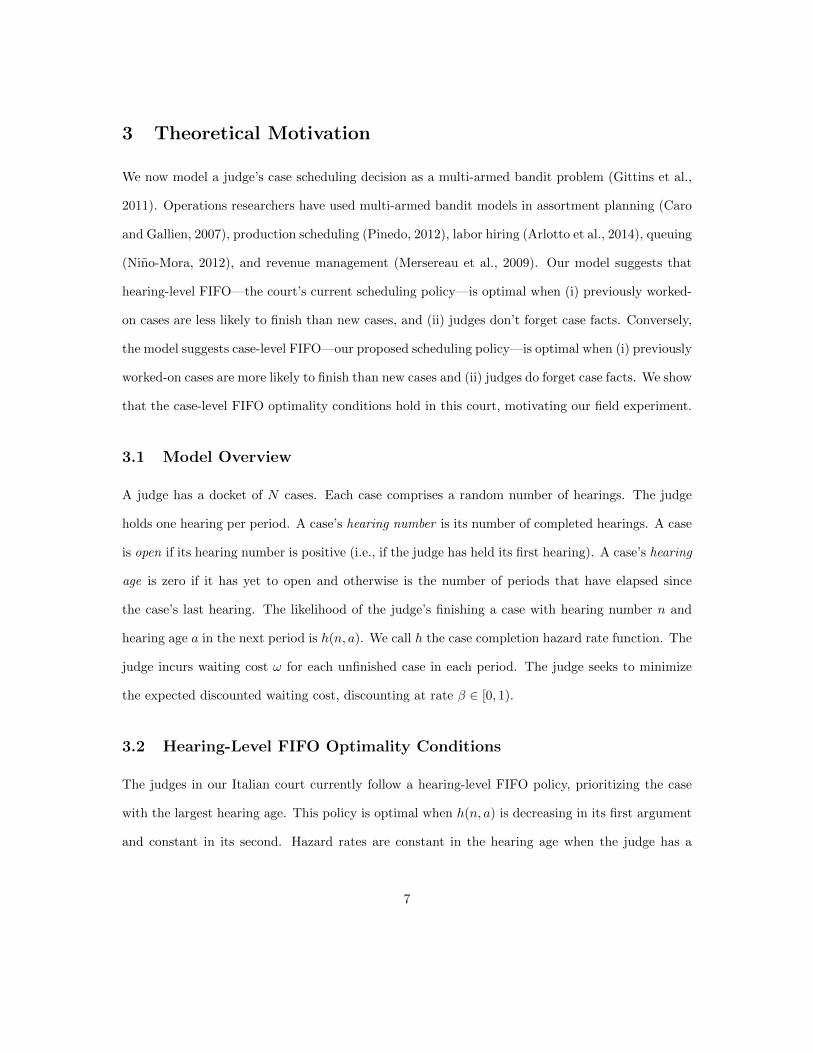
First, we find that the case completion hazard rate function increases in the hearing number.

The mean hazard rate—the fraction of hearings that complete a case—increases from .29 in the first

hearing to .37 in the second, to .45 in the third, and to .50 in the fourth. Each of these increases

is significant at the p = .01 level. And this pattern holds across case types: see Figure 1.2

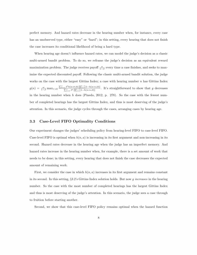
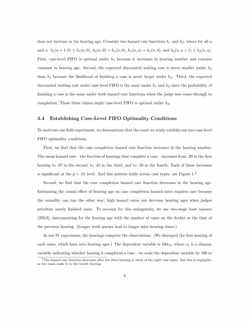
Second, we find that the case completion hazard rate function decreases in the hearing age.

Estimating the causal effect of hearing age on case completion hazard rates requires care because

the causality can run the other way; high hazard rates can decrease hearing ages when judges

prioritize nearly finished cases. To account for this endogeneity, we use two-stage least squares

(2SLS), instrumenting for the hearing age with the number of cases on the docket at the time of

the previous hearing. (Longer work queues lead to longer inter-hearing times.)

In our IV regressions, the hearings comprise the observations. (We disregard the first hearing of

each cases, which have zero hearing ages.) The dependent variable is 100ch, where ch is a dummy

variable indicating whether hearing h completed a case—we scale the dependent variable by 100 to

2The hazard rate function decreases after the third hearing in three of the eight case types. But this is negligible,as few cases make it to the fourth hearing.

9

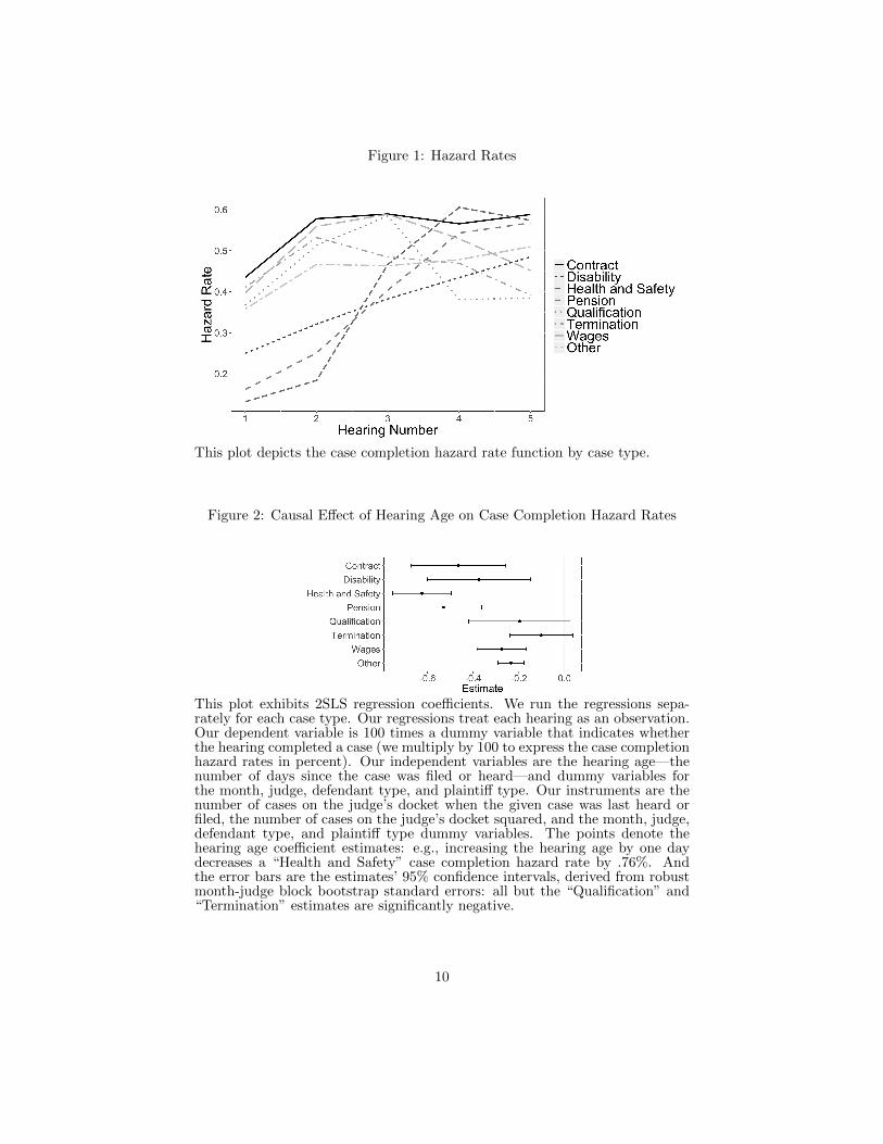
Figure 1: Hazard Rates

This plot depicts the case completion hazard rate function by case type.

Figure 2: Causal Effect of Hearing Age on Case Completion Hazard Rates

This plot exhibits 2SLS regression coefficients. We run the regressions sepa-rately for each case type. Our regressions treat each hearing as an observation.Our dependent variable is 100 times a dummy variable that indicates whetherthe hearing completed a case (we multiply by 100 to express the case completionhazard rates in percent). Our independent variables are the hearing age—thenumber of days since the case was filed or heard—and dummy variables forthe month, judge, defendant type, and plaintiff type. Our instruments are thenumber of cases on the judge’s docket when the given case was last heard orfiled, the number of cases on the judge’s docket squared, and the month, judge,defendant type, and plaintiff type dummy variables. The points denote thehearing age coefficient estimates: e.g., increasing the hearing age by one daydecreases a “Health and Safety” case completion hazard rate by .76%. Andthe error bars are the estimates’ 95% confidence intervals, derived from robustmonth-judge block bootstrap standard errors: all but the “Qualification” and“Termination” estimates are significantly negative.

10

express the hazard rate in percent. The independent variables are the hearing age—the number of

days since the case was previously heard—and dummy variables for the month, judge, defendant

type, and plaintiff type. The instrumental variables are the number of cases on the judge’s docket

when the given case was last heard or filed, the number of cases on the judge’s docket squared, and

the month, judge, defendant type, and plaintiff type dummy variables.

Figure 2 plots the hearing age regression coefficients by case type. The estimates are significantly

negative in six out eight case types; judges are less likely to finish cases they haven’t seen in a while.

This makes sense, as judges must forget case facts over time—it is impossible to perfectly recall

450 cases. For each case type, an F test rejects the null hypothesis of weak instrumental variables

at p = .01 Stock and Yogo (2005); and for each case type besides “Termination,” a Durbin-Wu-

Hausman test rejects the null hypothesis that the hearing ages are exogenous at p = .01 (Davidson

and Mackinnon, 2004, p. 237).

4 Field Experiment

Our theory suggests the Roman Labor Court of Appeals has been implementing FIFO along the

wrong dimension. According to our model, the court should follow case-level FIFO, the optimal

policy when judges forget case facts and the likelihood of finishing a case increases with the amount

of prior work. But it has been following hearing-level FIFO, the optimal policy when judges never

forget case facts and the likelihood of finishing a case decreases with the amount of prior work.

We will now test this theory with a field experiment that measures the effect of switching from

hearing-level FIFO to case-level FIFO. We use a difference-in-difference research design: six treated

judges switch from hearing-level to case-level FIFO on January 1, 2011, and 44 control judges follow

hearing-level FIFO throughout.

11

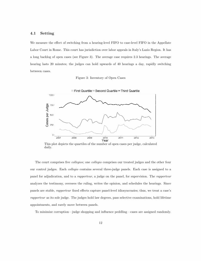
4.1 Setting

We measure the effect of switching from a hearing-level FIFO to case-level FIFO in the Appellate

Labor Court in Rome. This court has jurisdiction over labor appeals in Italy’s Lazio Region. It has

a long backlog of open cases (see Figure 3). The average case requires 2.3 hearings. The average

hearing lasts 20 minutes; the judges can hold upwards of 40 hearings a day, rapidly switching

between cases.

Figure 3: Inventory of Open Cases

This plot depicts the quartiles of the number of open cases per judge, calculateddaily.

The court comprises five collegios; one collegio comprises our treated judges and the other four

our control judges. Each collegio contains several three-judge panels. Each case is assigned to a

panel for adjudication, and to a rapporteur, a judge on the panel, for supervision. The rapporteur

analyzes the testimony, oversees the ruling, writes the opinion, and schedules the hearings. Since

panels are stable, rapporteur fixed effects capture panel-level idiosyncrasies; thus, we treat a case’s

rapporteur as its sole judge. The judges hold law degrees, pass selective examinations, hold lifetime

appointments, and rarely move between panels.

To minimize corruption—judge shopping and influence peddling—cases are assigned randomly.

12

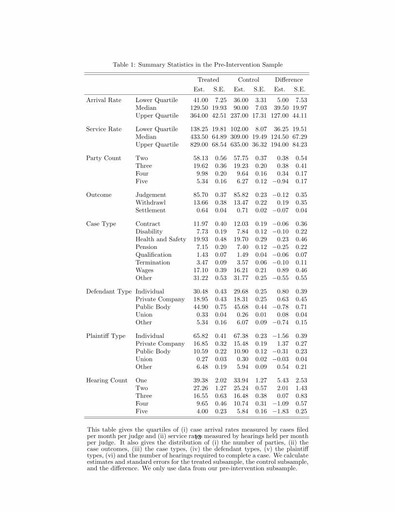
Table 1: Summary Statistics in the Pre-Intervention Sample

Treated Control Difference

Est. S.E. Est. S.E. Est. S.E.

Arrival Rate Lower Quartile 41.00 7.25 36.00 3.31 5.00 7.53Median 129.50 19.93 90.00 7.03 39.50 19.97Upper Quartile 364.00 42.51 237.00 17.31 127.00 44.11

Service Rate Lower Quartile 138.25 19.81 102.00 8.07 36.25 19.51Median 433.50 64.89 309.00 19.49 124.50 67.29Upper Quartile 829.00 68.54 635.00 36.32 194.00 84.23

Party Count Two 58.13 0.56 57.75 0.37 0.38 0.54Three 19.62 0.36 19.23 0.20 0.38 0.41Four 9.98 0.20 9.64 0.16 0.34 0.17Five 5.34 0.16 6.27 0.12 −0.94 0.17

Outcome Judgement 85.70 0.37 85.82 0.23 −0.12 0.35Withdrawl 13.66 0.38 13.47 0.22 0.19 0.35Settlement 0.64 0.04 0.71 0.02 −0.07 0.04

Case Type Contract 11.97 0.40 12.03 0.19 −0.06 0.36Disability 7.73 0.19 7.84 0.12 −0.10 0.22Health and Safety 19.93 0.48 19.70 0.29 0.23 0.46Pension 7.15 0.20 7.40 0.12 −0.25 0.22Qualification 1.43 0.07 1.49 0.04 −0.06 0.07Termination 3.47 0.09 3.57 0.06 −0.10 0.11Wages 17.10 0.39 16.21 0.21 0.89 0.46Other 31.22 0.53 31.77 0.25 −0.55 0.55

Defendant Type Individual 30.48 0.43 29.68 0.25 0.80 0.39Private Company 18.95 0.43 18.31 0.25 0.63 0.45Public Body 44.90 0.75 45.68 0.44 −0.78 0.71Union 0.33 0.04 0.26 0.01 0.08 0.04Other 5.34 0.16 6.07 0.09 −0.74 0.15

Plaintiff Type Individual 65.82 0.41 67.38 0.23 −1.56 0.39Private Company 16.85 0.32 15.48 0.19 1.37 0.27Public Body 10.59 0.22 10.90 0.12 −0.31 0.23Union 0.27 0.03 0.30 0.02 −0.03 0.04Other 6.48 0.19 5.94 0.09 0.54 0.21

Hearing Count One 39.38 2.02 33.94 1.27 5.43 2.53Two 27.26 1.27 25.24 0.57 2.01 1.43Three 16.55 0.63 16.48 0.38 0.07 0.83Four 9.65 0.46 10.74 0.31 −1.09 0.57Five 4.00 0.23 5.84 0.16 −1.83 0.25

This table gives the quartiles of (i) case arrival rates measured by cases filedper month per judge and (ii) service rates measured by hearings held per monthper judge. It also gives the distribution of (i) the number of parties, (ii) thecase outcomes, (iii) the case types, (iv) the defendant types, (v) the plaintifftypes, (vi) and the number of hearings required to complete a case. We calculateestimates and standard errors for the treated subsample, the control subsample,and the difference. We only use data from our pre-intervention subsample.

13

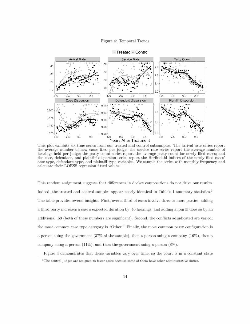
Figure 4: Temporal Trends

This plot exhibits six time series from our treated and control subsamples. The arrival rate series reportthe average number of new cases filed per judge; the service rate series report the average number ofhearings held per judge; the party count series report the average party count for newly filed cases; andthe case, defendant, and plaintiff dispersion series report the Herfindahl indices of the newly filed cases’case type, defendant type, and plaintiff type variables. We sample the series with monthly frequency andcalculate their LOESS regression fitted values.

This random assignment suggests that differences in docket compositions do not drive our results.

Indeed, the treated and control samples appear nearly identical in Table’s 1 summary statistics.3

The table provides several insights. First, over a third of cases involve three or more parties; adding

a third party increases a case’s expected duration by .40 hearings, and adding a fourth does so by an

additional .53 (both of these numbers are significant). Second, the conflicts adjudicated are varied;

the most common case type category is “Other.” Finally, the most common party configuration is

a person suing the government (37% of the sample), then a person suing a company (16%), then a

company suing a person (11%), and then the government suing a person (8%).

Figure 4 demonstrates that these variables vary over time, so the court is in a constant state

3The control judges are assigned to fewer cases because some of them have other administrative duties.

14

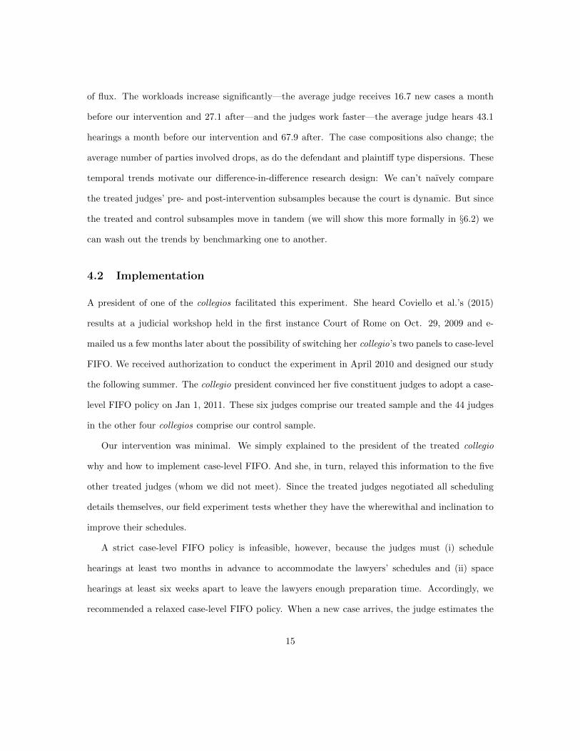
of flux. The workloads increase significantly—the average judge receives 16.7 new cases a month

before our intervention and 27.1 after—and the judges work faster—the average judge hears 43.1

hearings a month before our intervention and 67.9 after. The case compositions also change; the

average number of parties involved drops, as do the defendant and plaintiff type dispersions. These

temporal trends motivate our difference-in-difference research design: We can’t naıvely compare

the treated judges’ pre- and post-intervention subsamples because the court is dynamic. But since

the treated and control subsamples move in tandem (we will show this more formally in §6.2) we

can wash out the trends by benchmarking one to another.

4.2 Implementation

A president of one of the collegios facilitated this experiment. She heard Coviello et al.’s (2015)

results at a judicial workshop held in the first instance Court of Rome on Oct. 29, 2009 and e-

mailed us a few months later about the possibility of switching her collegio’s two panels to case-level

FIFO. We received authorization to conduct the experiment in April 2010 and designed our study

the following summer. The collegio president convinced her five constituent judges to adopt a case-

level FIFO policy on Jan 1, 2011. These six judges comprise our treated sample and the 44 judges

in the other four collegios comprise our control sample.

Our intervention was minimal. We simply explained to the president of the treated collegio

why and how to implement case-level FIFO. And she, in turn, relayed this information to the five

other treated judges (whom we did not meet). Since the treated judges negotiated all scheduling

details themselves, our field experiment tests whether they have the wherewithal and inclination to

improve their schedules.

A strict case-level FIFO policy is infeasible, however, because the judges must (i) schedule

hearings at least two months in advance to accommodate the lawyers’ schedules and (ii) space

hearings at least six weeks apart to leave the lawyers enough preparation time. Accordingly, we

recommended a relaxed case-level FIFO policy. When a new case arrives, the judge estimates the

15

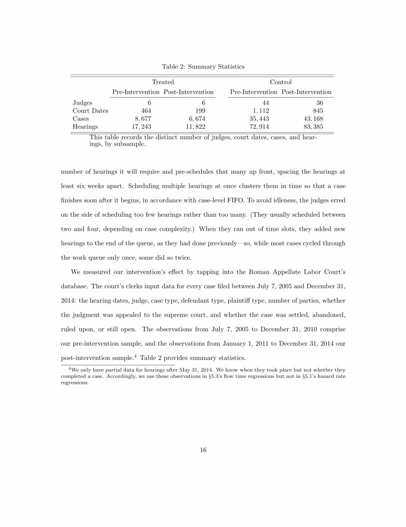
Table 2: Summary Statistics

Treated Control

Pre-Intervention Post-Intervention Pre-Intervention Post-Intervention

Judges 6 6 44 36Court Dates 464 199 1, 112 845Cases 8, 677 6, 674 35, 443 43, 168Hearings 17, 243 11, 822 72, 914 83, 385

This table records the distinct number of judges, court dates, cases, and hear-ings, by subsample.

number of hearings it will require and pre-schedules that many up front, spacing the hearings at

least six weeks apart. Scheduling multiple hearings at once clusters them in time so that a case

finishes soon after it begins, in accordance with case-level FIFO. To avoid idleness, the judges erred

on the side of scheduling too few hearings rather than too many. (They usually scheduled between

two and four, depending on case complexity.) When they ran out of time slots, they added new

hearings to the end of the queue, as they had done previously—so, while most cases cycled through

the work queue only once, some did so twice.

We measured our intervention’s effect by tapping into the Roman Appellate Labor Court’s

database. The court’s clerks input data for every case filed between July 7, 2005 and December 31,

2014: the hearing dates, judge, case type, defendant type, plaintiff type, number of parties, whether

the judgment was appealed to the supreme court, and whether the case was settled, abandoned,

ruled upon, or still open. The observations from July 7, 2005 to December 31, 2010 comprise

our pre-intervention sample, and the observations from January 1, 2011 to December 31, 2014 our

post-intervention sample.4 Table 2 provides summary statistics.

4We only have partial data for hearings after May 31, 2014. We know when they took place but not whether theycompleted a case. Accordingly, we use these observations in §5.3’s flow time regressions but not in §5.1’s hazard rateregressions.

16

5 Results

In this section, we report the effect of switching from hearing-level FIFO to case-level FIFO. Both

the control and treated judges appear less efficient in the post-intervention subsample because the

entire Italian judiciary got slower across our sample horizon (Coviello et al., 2012; Esposito et al.,

2014; CEPEJ, 2014a). But the treated judges are faster than they would have been had they tracked

the controls. Specifically, we estimate that our new scheduling policy (i) decreased the hazard rate

of case completion, (ii) decreased the inventory of open cases, (iii) decreased the case flow time,

and (iv) decreased the rate at which the judges’ rulings were appealed to the supreme court.

5.1 Hazard Rate Increase

Since case arrival rates are fixed, the only way switching from hearing-level FIFO to case-level FIFO

can decrease flow times is by reducing the inventory of open cases. To transition from high- to low-

inventory regimes, case outflows must temporarily exceed case inflows. Thus, while a scheduling

policy change won’t affect long-run case completion rates, which track the exogenous arrival rates,

it should increase short-run completion rates as the firm burns through excess stock.

There are only two ways to increase the case completion rate: increase the service rate—the

number of hearings per day—or increase the hazard rate of case completion—the likelihood of a

given hearing concluding a case (i.e., the ratio of cases completed to hearings held). Since our

intervention cannot influence the service rate, which is independent of case sequencing, it must

reduce inventories via the hazard rate. Thus, the hazard rate of case completion mediates our

intervention’s effect. The only way switching to case-level FIFO can decrease flow times is by

moving high-hazard hearings—those likely to finish a case—to the front of the queue.

We establish that our intervention increased the treated judges’ hazard rates with difference-in-

difference regressions. We consider four statistical models, regressing with random and fixed effects,

and with and without controls. For the control-free random effects specification, we regress 100ch

17

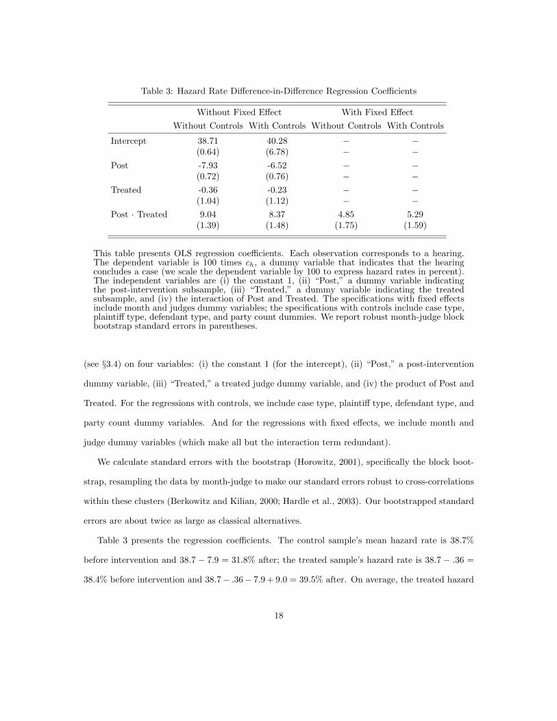
Table 3: Hazard Rate Difference-in-Difference Regression Coefficients

Without Fixed Effect With Fixed Effect

Without Controls With Controls Without Controls With Controls

Intercept 38.71 40.28 − −(0.64) (6.78) − −

Post -7.93 -6.52 − −(0.72) (0.76) − −

Treated -0.36 -0.23 − −(1.04) (1.12) − −

Post · Treated 9.04 8.37 4.85 5.29(1.39) (1.48) (1.75) (1.59)

This table presents OLS regression coefficients. Each observation corresponds to a hearing.The dependent variable is 100 times ch, a dummy variable that indicates that the hearingconcludes a case (we scale the dependent variable by 100 to express hazard rates in percent).The independent variables are (i) the constant 1, (ii) “Post,” a dummy variable indicatingthe post-intervention subsample, (iii) “Treated,” a dummy variable indicating the treatedsubsample, and (iv) the interaction of Post and Treated. The specifications with fixed effectsinclude month and judges dummy variables; the specifications with controls include case type,plaintiff type, defendant type, and party count dummies. We report robust month-judge blockbootstrap standard errors in parentheses.

(see §3.4) on four variables: (i) the constant 1 (for the intercept), (ii) “Post,” a post-intervention

dummy variable, (iii) “Treated,” a treated judge dummy variable, and (iv) the product of Post and

Treated. For the regressions with controls, we include case type, plaintiff type, defendant type, and

party count dummy variables. And for the regressions with fixed effects, we include month and

judge dummy variables (which make all but the interaction term redundant).

We calculate standard errors with the bootstrap (Horowitz, 2001), specifically the block boot-

strap, resampling the data by month-judge to make our standard errors robust to cross-correlations

within these clusters (Berkowitz and Kilian, 2000; Hardle et al., 2003). Our bootstrapped standard

errors are about twice as large as classical alternatives.

Table 3 presents the regression coefficients. The control sample’s mean hazard rate is 38.7%

before intervention and 38.7 − 7.9 = 31.8% after; the treated sample’s hazard rate is 38.7 − .36 =

38.4% before intervention and 38.7− .36− 7.9 + 9.0 = 39.5% after. On average, the treated hazard

18

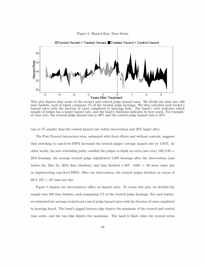
Figure 5: Hazard Rate Time Series

This plot depicts time series of the treated and control judge hazard rates. We divide the data into 100time buckets, each of which comprises 1% of the treated judge hearings. We then calculate each bucket’shazard rates with the fraction of cases completed to hearings held. The band’s color indicates whichsample of judges has a larger hazard rate, and the band’s thickness indicates by how much. For example,at time zero, the treated judge hazard rate is 49% and the control judge hazard rate is 35%.

rate is 1% smaller than the control hazard rate before intervention and 28% larger after.

The Post·Treated interaction term, estimated with fixed effects and without controls, suggests

that switching to case-level FIFO increased the treated judges’ average hazard rate by 4.85%. In

other words, the new scheduling policy enabled the judges to finish an extra case every 100/4.85 =

20.6 hearings; the average treated judge adjudicated 1,807 hearings after the intervention (and

before the May 31, 2014 data blackout) and thus finished 1, 807 · .0485 = 88 more cases due

to implementing case-level FIFO. After the intervention, the treated judges finished an excess of

88/1, 247 = .07 cases per day.

Figure 5 depicts our intervention’s effect on hazard rates. To create this plot, we divided the

sample into 100 time buckets, each comprising 1% of the treated judge hearings. For each bucket,

we estimated the average treated and control judge hazard rates with the fraction of cases completed

to hearings heard. The band’s jagged bottom edge depicts the minimum of the treated and control

time series, and the top edge depicts the maximum. The band is black when the treated series

19

is larger, and gray when the control series is larger. The treated and control hazard rates mirror

one another for five years before treatment—the band is thin with equal parts gray and black—but

diverge soon thereafter; the band turns thick and black.

5.2 Inventory Decrease

Since hazard rates mediate our intervention’s effect, we calculate the inventory decrease attributable

to the hazard rate increases; doing so controls for unrelated arrival and service rate changes. Specif-

ically, Figure 6 plots the reduction in case inventories over time attributable to the treated judges’

abnormal hazard rates. To create this figure, we pair each treated judge with a counterfactual

judge, who mirrors his counterpart in every way but one: the hazard rate. A counterfactual judge’s

hazard rate tracks the monthly average control judge hazard rate. For example, if a treated judge

finishes 35 cases out of 80 hearings in a month and the control judges collectively finish 450 cases

out of 1,200 hearings, then the corresponding counterfactual judge finishes (450/1, 200) · 80 = 30

cases, and the treated judge’s inventory falls by 35 − 30 = 5 cases relative to the counterfactual.

The graph depicts the mean deviation between the counterfactual judges’ simulated inventories and

the treated judges’ true inventories. We normalize the difference to zero at the intervention date

and bootstrap for 90% confidence intervals.

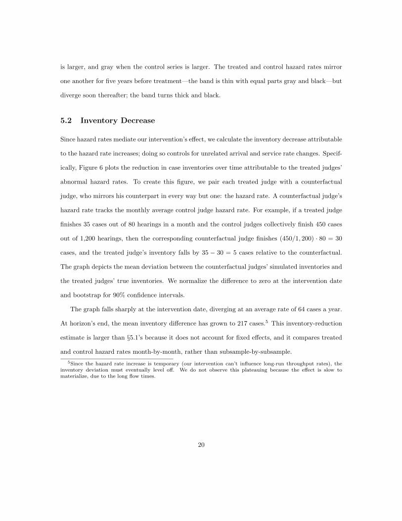
The graph falls sharply at the intervention date, diverging at an average rate of 64 cases a year.

At horizon’s end, the mean inventory difference has grown to 217 cases.5 This inventory-reduction

estimate is larger than §5.1’s because it does not account for fixed effects, and it compares treated

and control hazard rates month-by-month, rather than subsample-by-subsample.

5Since the hazard rate increase is temporary (our intervention can’t influence long-run throughput rates), theinventory deviation must eventually level off. We do not observe this plateauing because the effect is slow tomaterialize, due to the long flow times.

20

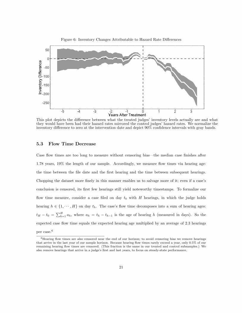
Figure 6: Inventory Changes Attributable to Hazard Rate Differences

This plot depicts the difference between what the treated judges’ inventory levels actually are and whatthey would have been had their hazard rates mirrored the control judges’ hazard rates. We normalize theinventory difference to zero at the intervention date and depict 90% confidence intervals with gray bands.

5.3 Flow Time Decrease

Case flow times are too long to measure without censoring bias—the median case finishes after

1.78 years, 19% the length of our sample. Accordingly, we measure flow times via hearing age:

the time between the file date and the first hearing and the time between subsequent hearings.

Chopping the dataset more finely in this manner enables us to salvage more of it; even if a case’s

conclusion is censored, its first few hearings still yield noteworthy timestamps. To formalize our

flow time measure, consider a case filed on day t0 with H hearings, in which the judge holds

hearing h ∈ {1, · · · , H} on day th. The case’s flow time decomposes into a sum of hearing ages:

tH − t0 =∑Hh=1 ah, where ah = th − th−1 is the age of hearing h (measured in days). So the

expected case flow time equals the expected hearing age multiplied by an average of 2.3 hearings

per case.6

6Hearing flow times are also censored near the end of our horizon; to avoid censoring bias we remove hearingsthat arrive in the last year of our sample horizon. Because hearing flow times rarely exceed a year, only 0.5% of ourremaining hearing flow times are censored. (This fraction is the same in our treated and control subsamples.) Wealso remove hearings that arrive in a judge’s first and last years, to focus on steady-state performance.

21

Table 4: Flow Time Difference-in-Difference Regression Coefficients

Without Fixed Effect With Fixed Effect

Without Controls With Controls Without Controls With Controls

Intercept 264.22 448.60 − −(2.82) (30.25) − −

Post 71.48 66.00 − −(5.19) (5.24) − −

Treated 68.57 66.49 − −(9.42) (9.76) − −

Post · Treated -48.14 -46.06 -46.68 -42.55(13.65) (13.84) (6.98) (7.43)

This table presents OLS regression coefficients. Each observation corresponds to a hearing.The dependent variable is flow time age ah, the number of days between a case’s currenthearing and its previous hearing (or file date if it is the first hearing). The independentvariables, controls, and fixed effects are as described in Table 3.

We establish that our intervention decreased the treated judges’ flow times with difference-in-

difference regressions similar to §5.1’s. The only difference is that the dependent variable changes

to hearing age ah.

Table 4 presents the regression coefficients. The control hearing flow times average 264 days

before intervention and 264+71 = 336 days after; the treated hearing flow times average 264+69 =

333 days before intervention and 264 + 71 + 69− 48 = 356 after. The Post·Treated interaction term

suggests that adopting case-level FIFO decreased the average treated judges’ hearing flow time by

48 days and case flow time by 48.1 · 2.3 = 111 days (12%). Note, this is actually a lower bound

on the steady-state flow time decrease because transitioning to the efficient regime took time (see

Figure 6).

5.4 Appeals Rate Decrease

About a year after our intervention, the treated judges reported a serendipitous side effect: They

forgot fewer case facts under case-level FIFO due to the reduced time between hearings. They

speculated that better remembering the cases led to fairer rulings. Accordingly, we test whether

22

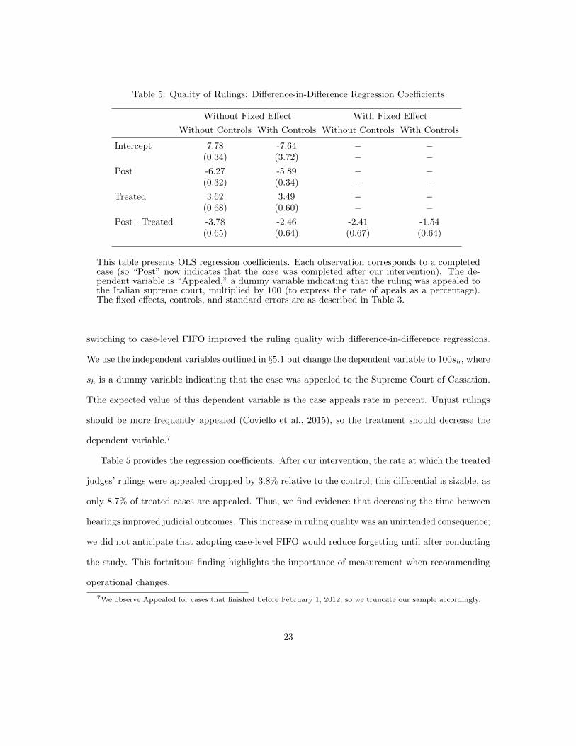
Table 5: Quality of Rulings: Difference-in-Difference Regression Coefficients

Without Fixed Effect With Fixed Effect

Without Controls With Controls Without Controls With Controls

Intercept 7.78 -7.64 − −(0.34) (3.72) − −

Post -6.27 -5.89 − −(0.32) (0.34) − −

Treated 3.62 3.49 − −(0.68) (0.60) − −

Post · Treated -3.78 -2.46 -2.41 -1.54(0.65) (0.64) (0.67) (0.64)

This table presents OLS regression coefficients. Each observation corresponds to a completedcase (so “Post” now indicates that the case was completed after our intervention). The de-pendent variable is “Appealed,” a dummy variable indicating that the ruling was appealed tothe Italian supreme court, multiplied by 100 (to express the rate of apeals as a percentage).The fixed effects, controls, and standard errors are as described in Table 3.

switching to case-level FIFO improved the ruling quality with difference-in-difference regressions.

We use the independent variables outlined in §5.1 but change the dependent variable to 100sh, where

sh is a dummy variable indicating that the case was appealed to the Supreme Court of Cassation.

Tthe expected value of this dependent variable is the case appeals rate in percent. Unjust rulings

should be more frequently appealed (Coviello et al., 2015), so the treatment should decrease the

dependent variable.7

Table 5 provides the regression coefficients. After our intervention, the rate at which the treated

judges’ rulings were appealed dropped by 3.8% relative to the control; this differential is sizable, as

only 8.7% of treated cases are appealed. Thus, we find evidence that decreasing the time between

hearings improved judicial outcomes. This increase in ruling quality was an unintended consequence;

we did not anticipate that adopting case-level FIFO would reduce forgetting until after conducting

the study. This fortuitous finding highlights the importance of measurement when recommending

operational changes.

7We observe Appealed for cases that finished before February 1, 2012, so we truncate our sample accordingly.

23

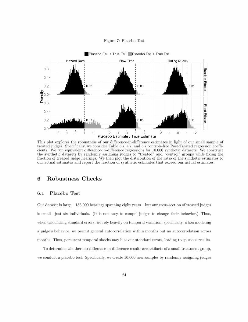
Figure 7: Placebo Test

This plot explores the robustness of our difference-in-difference estimates in light of our small sample oftreated judges. Specifically, we consider Table 3’s, 4’s, and 5’s controls-free Post·Treated regression coeffi-cients. We run equivalent difference-in-difference regressions for 10,000 synthetic datasets. We constructthe synthetic datasets by randomly assigning judges to “treated” and “control” groups while fixing thefraction of treated judge hearings. We then plot the distribution of the ratio of the synthetic estimates toour actual estimates and report the fraction of synthetic estimates that exceed our actual estimates.

6 Robustness Checks

6.1 Placebo Test

Our dataset is large—185,000 hearings spanning eight years—but our cross-section of treated judges

is small—just six individuals. (It is not easy to compel judges to change their behavior.) Thus,

when calculating standard errors, we rely heavily on temporal variation; specifically, when modeling

a judge’s behavior, we permit general autocorrelation within months but no autocorrelation across

months. Thus, persistent temporal shocks may bias our standard errors, leading to spurious results.

To determine whether our difference-in-difference results are artifacts of a small treatment group,

we conduct a placebo test. Specifically, we create 10,000 new samples by randomly assigning judges

24

to “treated” and “control” groups; the case compositions, intervention date, and proportion of

treated hearings remain fixed. For each sample, we run the control-free hazard rate, flow time, and

ruling quality difference-in-difference regressions from Tables 3, 4, and 5.

Figure 7 plots histograms of the Post·Treated coefficients, where the real estimates are normal-

ized to one. Our true random effects estimates stand out relative to the simulations: Out of 10,000

simulations, only 14 are stronger in both hazard and flow time, and only one is stronger in hazard

rate, flow time, and ruling quality. And our true fixed effects estimates, although weaker, are also

noteworthy: Out of 10,000 simulations, only 368 are stronger in both hazard and flow time, and

only 19 are stronger in hazard rate, flow time, and ruling quality. These results suggest our findings

are not artifacts of a small treatment group.

6.2 Parallel Trends

For our difference-in-difference estimates to be valid, the treated and control hazard rates must

exhibit parallel trend lines before intervention (Angrist and Pischke, 2009, p. 230); the control

sample would be a poor benchmark if it did not track the treated sample, pre-intervention. We

test the parallel trends hypothesis by regressing our pre-intervention dependent variables on (i) the

constant 1, (ii) “Time,” the number of centuries after the intervention (we use this timescale to

scale up the regression coefficients), (iii) Treated, and (iv) the product of Time and Treated.

Table 6 tabulates the regression coefficients. The Time·Treated coefficient is statistically in-

significant for hazard rate, flow time, and ruling quality dependent variables. Thus, we fail to reject

the hypothesis that the treated and control hazard rates follow the same trend lines before our

intervention.

6.3 Self-Selection

Our treated subsample should be a fairly representative cross section of the court because: (i) the

judges did not elect to participate in the study; instead, they were cajoled to join by the president

25

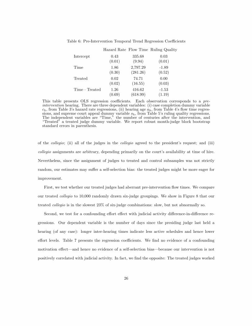
Table 6: Pre-Intervention Temporal Trend Regression Coefficients

Hazard Rate Flow Time Ruling Quality

Intercept 0.43 335.68 0.03(0.01) (9.94) (0.01)

Time 1.86 2,797.29 -1.89(0.30) (281.26) (0.52)

Treated 0.02 74.71 0.00(0.02) (16.55) (0.03)

Time · Treated 1.26 416.62 -1.53(0.69) (618.99) (1.19)

This table presents OLS regression coefficients. Each observation corresponds to a pre-intervention hearing. There are three dependent variables: (i) case completion dummy variablech, from Table 3’s hazard rate regressions, (ii) hearing age ah, from Table 4’s flow time regres-sions, and supreme court appeal dummy variable sh, from Table 5’s ruling quality regressions.The independent variables are “Time,” the number of centuries after the intervention, and“Treated” a treated judge dummy variable. We report robust month-judge block bootstrapstandard errors in parenthesis.

of the collegio; (ii) all of the judges in the collegio agreed to the president’s request; and (iii)

collegio assignments are arbitrary, depending primarily on the court’s availability at time of hire.

Nevertheless, since the assignment of judges to treated and control subsamples was not strictly

random, our estimates may suffer a self-selection bias: the treated judges might be more eager for

improvement.

First, we test whether our treated judges had aberrant pre-intervention flow times. We compare

our treated collegio to 10,000 randomly drawn six-judge groupings. We show in Figure 8 that our

treated collegio is in the slowest 23% of six-judge combinations: slow, but not abnormally so.

Second, we test for a confounding effort effect with judicial activity difference-in-difference re-

gressions. Our dependent variable is the number of days since the presiding judge last held a

hearing (of any case): longer inter-hearing times indicate less active schedules and hence lower

effort levels. Table 7 presents the regression coefficients. We find no evidence of a confounding

motivation effect—and hence no evidence of a self-selection bias—because our intervention is not

positively correlated with judicial activity. In fact, we find the opposite: The treated judges worked

26

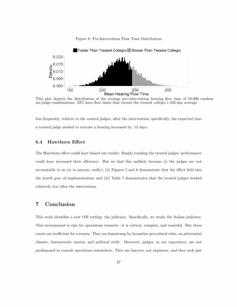
Figure 8: Pre-Intervention Flow Time Distribution

This plot depicts the distribution of the average pre-intervention hearing flow time of 10,000 randomsix-judge combinations: 23% have flow times that exceed the treated collegio’s 245-day average.

less frequently, relative to the control judges, after the intervention; specifically, the expected time

a treated judge needed to execute a hearing increased by .13 days.

6.4 Hawthorn Effect

The Hawthorn effect could have biased our results: Simply tracking the treated judges’ performance

could have increased their efficiency. But we find this unlikely because (i) the judges are not

accountable to us (or to anyone, really); (ii) Figures 5 and 6 demonstrate that the effect held into

the fourth year of implementation; and (iii) Table 7 demonstrates that the treated judges worked

relatively less after the intervention.

7 Conclusion

This work identifies a new OM setting: the judiciary. Specifically, we study the Italian judiciary.

This environment is ripe for operations research—it is critical, complex, and wasteful. But these

courts are inefficient for a reason: They are hamstrung by byzantine procedural rules, an adversarial

climate, bureaucratic inertia, and political strife. Moreover, judges, in our experience, are not

predisposed to consult operations researchers. They are lawyers, not engineers, and they seek just

27

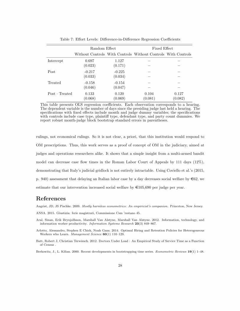
Table 7: Effort Levels: Difference-in-Difference Regression Coefficients

Random Effect Fixed Effect

Without Controls With Controls Without Controls With Controls

Intercept 0.697 1.127 − −(0.023) (0.171) − −

Post -0.217 -0.225 − −(0.033) (0.034) − −

Treated -0.158 -0.154 − −(0.046) (0.047) − −

Post · Treated 0.133 0.120 0.104 0.127(0.068) (0.069) (0.081) (0.082)

This table presents OLS regression coefficients. Each observation corresponds to a hearing.The dependent variable is the number of days since the presiding judge last held a hearing. Thespecifications with fixed effects include month and judge dummy variables; the specificationswith controls include case type, plaintiff type, defendant type, and party count dummies. Wereport robust month-judge block bootstrap standard errors in parentheses.

rulings, not economical rulings. So it is not clear, a priori, that this institution would respond to

OM prescriptions. Thus, this work serves as a proof of concept of OM in the judiciary, aimed at

judges and operations researchers alike. It shows that a simple insight from a multi-armed bandit

model can decrease case flow times in the Roman Labor Court of Appeals by 111 days (12%),

demonstrating that Italy’s judicial gridlock is not entirely intractable. Using Coviello et al.’s (2015,

p. 940) assessment that delaying an Italian labor case by a day decreases social welfare by e62, we

estimate that our intervention increased social welfare by e105,690 per judge per year.

ReferencesAngrist, JD, JS Pischke. 2009. Mostly harmless econometrics: An empiricist’s companion. Princeton, New Jersey.

ANSA. 2015. Giustizia: ferie magistrati, Commissione Csm ’restano 45.

Aral, Sinan, Erik Brynjolfsson, Marshall Van Alstyne, Marshall Van Alstyne. 2012. Information, technology, andinformation worker productivity. Information Systems Research 23(3) 849–867.

Arlotto, Alessandro, Stephen E Chick, Noah Gans. 2014. Optimal Hiring and Retention Policies for HeterogeneousWorkers who Learn. Management Science 60(1) 110–129.

Batt, Robert J, Christian Terwiesch. 2012. Doctors Under Load : An Empirical Study of Service Time as a Functionof Census .

Berkowitz, J., L. Kilian. 2000. Recent developments in bootstrapping time series. Econometric Reviews 19(1) 1–48.

28

Caro, Felipe, Jeremie Gallien. 2007. Dynamic Assortment with Demand Learning for Seasonal Consumer Goods.Management Science 53(2) 276–292.

CEPEJ. 2006. Compendium of best practices on time management of judicial proceedings. Tech. rep., EuropeanCommission for the Efficiency of Justice, CEPEJ2006.

CEPEJ. 2014a. European judicial systems Edition 2014: efficiency and quality of justice. Tech. rep.

CEPEJ. 2014b. Report on European Judicial Systems Edition 2014 (2012 Data): Efficiency and Quality of Justice2014.

Chirico, Annalisa. 2013. Le toghe e i 51 giorni di ferie: confessioni di un magistrato.

Coviello, Decio, Andrea Ichino, Nicola Persico. 2012. Time allocation and task juggling (preliminary draft) 104(2)1–26.

Coviello, Decio, Andrea Ichino, Nicola Persico. 2014. Time allocation and task juggling. American Economic Review104(2) 609–623.

Coviello, Decio, Andrea Ichino, Nicola Persico. 2015. The inefficiency of worker time use. Journal of the EuropeanEconomic Association 13(October 2015) 906–947.

Davidson, Russell, James G Mackinnon. 2004. Econometric Theory and Methods, vol. 21. Oxford University Press,New York, NY.

Esposito, G, MS Lanau, S Pompe. 2014. Judicial system reform in italy-A key to growth.

Freeman, Michael, Nicos Savva, Stefan Scholtes. 2015. Gatekeepers at Work : An Empirical Analysis of a MaternityUnit 1–38.

Gittins, John, Kevin Glazebrook, Richard Weber. 2011. Multi-Armed Bandit Allocation Indices: 2nd Edition. JohnWiley and Sons.

Hardle, W., J. Horowitz, J. P. Kreiss. 2003. Bootstrap methods for time series. International Statistical Review435–459.

Horowitz, J. L. 2001. The bootstrap. Handbook of econometrics 5 3159–3228.

Kc, D. S., C. Terwiesch. 2009. Impact of Workload on Service Time and Patient Safety: An Econometric Analysisof Hospital Operations. Management Science 55(9) 1486–1498.

Kc, Diwas. 2014. Does multitasking improve performance? Evidence from the emergency department. Manufacturing& Service Operations Management 16(2) 168–183.

Mersereau, Adam J., Paat Rusmevichientong, John N. Tsitsiklis. 2009. A structured multiarmed bandit problemand the greedy policy. IEEE Transactions on Automatic Control 54(12) 2787–2802.

Nino-Mora, Jose. 2012. Towards minimum loss job routing to parallel heterogeneous multiserver queues via indexpolicies. European Journal of Operational Research 220(3) 705–715.

OECD. 2013. What makes civil justice effective? Tech. Rep. 18, OECD Economics Department Policy Notes.

Pinedo, Michael. 2012. Scheduling: theory, algorithms, and systems. Springer, New York, NY.

Powell, a., S. Savin, N. Savva. 2012. Physician Workload and Hospital Reimbursement: Overworked PhysiciansGenerate Less Revenue per Patient. Manufacturing & Service Operations Management 14(4) 512–528.

Staats, B. R. BR, F. Gino. 2012. Specialization and Variety in Repetitive Tasks: Evidence from a Japanese Bank.Management Science 58(February 2015) 1141–1159.

Stock, James H, Motohiro Yogo. 2005. Testing for weak instruments in linear IV regression. Identification andinference for econometric models: Essays in honor of Thomas Rothenberg .

29

Tan, Tom F, Serguei Netessine. 2014. When Does the Devil Make Work? An Empirical Study of the Impact ofWorkload on Worker Productivity. Management Science 60(6) 1574–1593.

Unita’ per la Costituzione. 2015. Internal Memo.

Wang, Lu, Itai Gurvich, Jan A. Van Mieghem, Kevin J. O’Leary. 2015. Task Switching and Productivity in Collab-orative Work: A Field Study of Hospitalists.

World Bank Group. 2014. Doing Business Report: Enforcing Contracts.

30