Embed Size (px)
Citation preview
Multivariate Analyses with
manova and GLM
Alan Taylor, Department of Psychology Macquarie University
2002-2011
© Macquarie University 2002-2011

Contents i
Introduction 1
1. Background to Multivariate Analysis of Variance 3 1.1 Between-and Within-Group Sums of Squares: the SSCP Matrices 3 1.2 The Determinant, the Variance of SSCP Matrices, and Wilks' Lambda 6 1.3 Differentiating Between Groups with the Discriminant Function – A Weighted Composite Variable 8 1.4 Choosing the Weights: Eigenvalues and Eigenvectors 10 1.4.1 The Eigenvalues and Eigenvectors of a Correlation Matrix 10 1.4.2 The Eigenvalues and Eigenvectors of the W -1B Matrix 11 1.5 What Affects Eigenvalues and Multivariate Statistics 13 1.6 Multivariate Statistics 15 1.7 Multivariate Analysis in SPSS 16 1.8 The Main Points 17 2. Multivariate Analysis with the GLM procedure 19 2.1 The Dataset 19 2.2 Using GLM for a Multivariate Analysis 20 2.3 Assumptions in Multivariate Analysis of Variance 24 2.3.1 Homogeneity 24 2.3.2 Normality 25 2.4 Conclusion 28
3. Multivariate Analysis with the manova procedure 29 3.1 Conclusion 35
Contents ii
4. Following up a Multivariate Analysis of Variance 37 4.1 Multivariate Comparisons of Groups 37 4.2 The "Significance to Remove" of Each Dependent Variable 46
5. Using a Numeric Independent Variable in a Multivariate Analysis 49
6. Measures of Multivariate Effect Size 51 7. The Multivariate Approach to Repeated Measures 53 7.1 Profile Analysis 54
8. Doubly Multivariate Analyses 57
9. Some Issues and Further Reading 61 9.1 Univariate or Multivariate? 61 9.2 Following up a Significant Multivariate Result 61 9.3 Power 62 References 64
Appendix 1. Eigen Analysis of the Y1, Y2 Data in Section 1.5.2 65
Appendix 2. Obtaining the Determinants of the W and T Matrices Using the SPSS Matrix Procedure 66
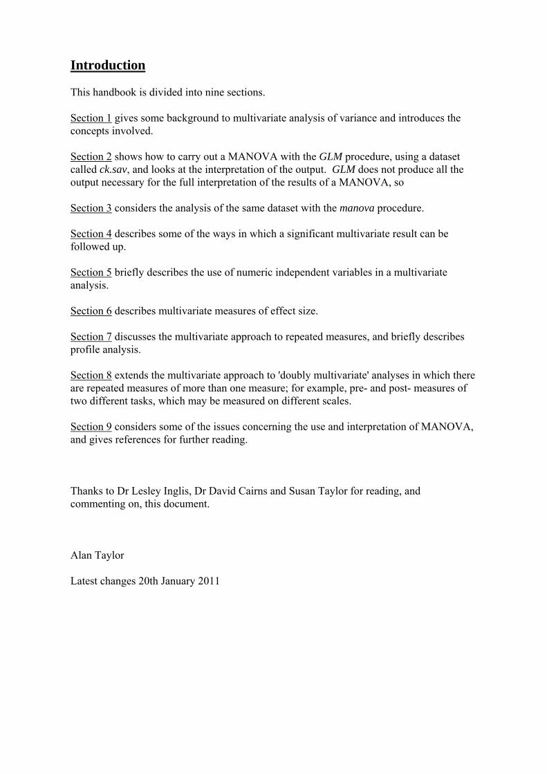
Introduction This handbook is divided into nine sections. Section 1 gives some background to multivariate analysis of variance and introduces the concepts involved. Section 2 shows how to carry out a MANOVA with the GLM procedure, using a dataset called ck.sav, and looks at the interpretation of the output. GLM does not produce all the output necessary for the full interpretation of the results of a MANOVA, so Section 3 considers the analysis of the same dataset with the manova procedure. Section 4 describes some of the ways in which a significant multivariate result can be followed up. Section 5 briefly describes the use of numeric independent variables in a multivariate analysis. Section 6 describes multivariate measures of effect size. Section 7 discusses the multivariate approach to repeated measures, and briefly describes profile analysis. Section 8 extends the multivariate approach to 'doubly multivariate' analyses in which there are repeated measures of more than one measure; for example, pre- and post- measures of two different tasks, which may be measured on different scales. Section 9 considers some of the issues concerning the use and interpretation of MANOVA, and gives references for further reading. Thanks to Dr Lesley Inglis, Dr David Cairns and Susan Taylor for reading, and commenting on, this document. Alan Taylor Latest changes 20th January 2011

1. Background 3
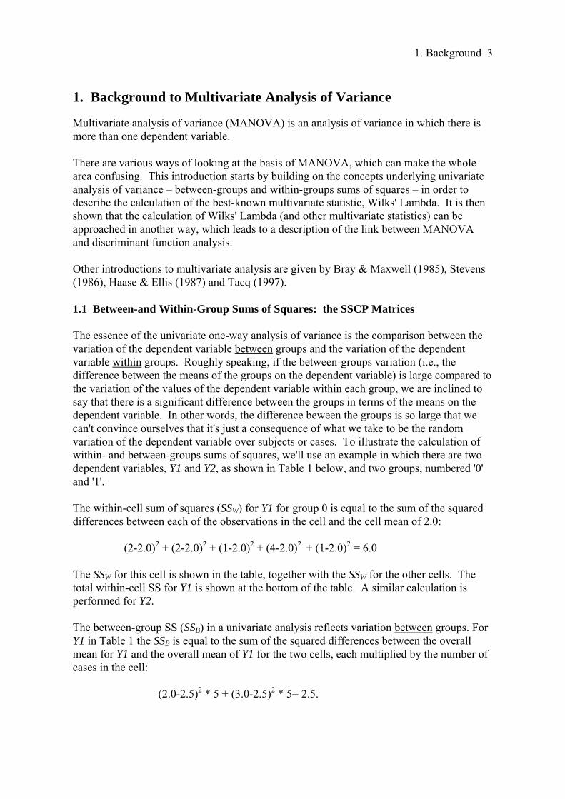
1. Background to Multivariate Analysis of Variance Multivariate analysis of variance (MANOVA) is an analysis of variance in which there is more than one dependent variable. There are various ways of looking at the basis of MANOVA, which can make the whole area confusing. This introduction starts by building on the concepts underlying univariate analysis of variance – between-groups and within-groups sums of squares – in order to describe the calculation of the best-known multivariate statistic, Wilks' Lambda. It is then shown that the calculation of Wilks' Lambda (and other multivariate statistics) can be approached in another way, which leads to a description of the link between MANOVA and discriminant function analysis. Other introductions to multivariate analysis are given by Bray & Maxwell (1985), Stevens (1986), Haase & Ellis (1987) and Tacq (1997). 1.1 Between-and Within-Group Sums of Squares: the SSCP Matrices The essence of the univariate one-way analysis of variance is the comparison between the variation of the dependent variable between groups and the variation of the dependent variable within groups. Roughly speaking, if the between-groups variation (i.e., the difference between the means of the groups on the dependent variable) is large compared to the variation of the values of the dependent variable within each group, we are inclined to say that there is a significant difference between the groups in terms of the means on the dependent variable. In other words, the difference beween the groups is so large that we can't convince ourselves that it's just a consequence of what we take to be the random variation of the dependent variable over subjects or cases. To illustrate the calculation of within- and between-groups sums of squares, we'll use an example in which there are two dependent variables, Y1 and Y2, as shown in Table 1 below, and two groups, numbered '0' and '1'. The within-cell sum of squares (SSW) for Y1 for group 0 is equal to the sum of the squared differences between each of the observations in the cell and the cell mean of 2.0: (2-2.0)2 + (2-2.0)2 + (1-2.0)2 + (4-2.0)2 + (1-2.0)2 = 6.0 The SSW for this cell is shown in the table, together with the SSW for the other cells. The total within-cell SS for Y1 is shown at the bottom of the table. A similar calculation is performed for Y2. The between-group SS (SSB) in a univariate analysis reflects variation between groups. For Y1 in Table 1 the SSB is equal to the sum of the squared differences between the overall mean for Y1 and the overall mean of Y1 for the two cells, each multiplied by the number of cases in the cell: (2.0-2.5)2 * 5 + (3.0-2.5)2 * 5= 2.5.
1. Background 4
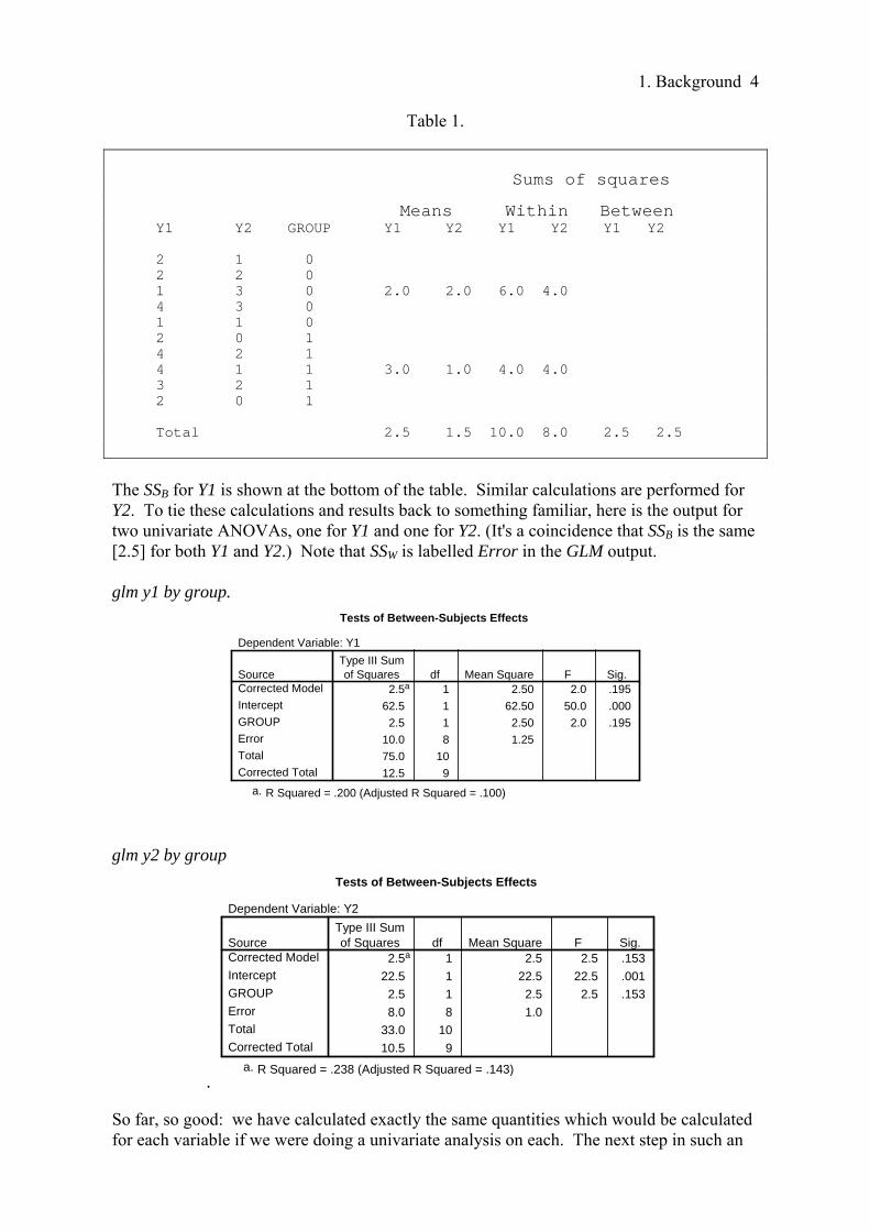
Table 1.
Sums of squares
Means Within Between Y1 Y2 GROUP Y1 Y2 Y1 Y2 Y1 Y2 2 1 0 2 2 0 1 3 0 2.0 2.0 6.0 4.0 4 3 0 1 1 0 2 0 1 4 2 1 4 1 1 3.0 1.0 4.0 4.0 3 2 1 2 0 1 Total 2.5 1.5 10.0 8.0 2.5 2.5
The SSB for Y1 is shown at the bottom of the table. Similar calculations are performed for Y2. To tie these calculations and results back to something familiar, here is the output for two univariate ANOVAs, one for Y1 and one for Y2. (It's a coincidence that SSB is the same [2.5] for both Y1 and Y2.) Note that SSW is labelled Error in the GLM output. glm y1 by group.
Tests of Between-Subjects Effects
Dependent Variable: Y1
2.5a 1 2.50 2.0 .195
62.5 1 62.50 50.0 .000
2.5 1 2.50 2.0 .195
10.0 8 1.25
75.0 10
12.5 9
SourceCorrected Model
Intercept
GROUP
Error
Total
Corrected Total
Type III Sumof Squares df Mean Square F Sig.
R Squared = .200 (Adjusted R Squared = .100)a.
glm y2 by group
.
Tests of Between-Subjects Effects
Dependent Variable: Y2
2.5a 1 2.5 2.5 .153
22.5 1 22.5 22.5 .001
2.5 1 2.5 2.5 .153
8.0 8 1.0
33.0 10
10.5 9
SourceCorrected Model
Intercept
GROUP
Error
Total
Corrected Total
Type III Sumof Squares df Mean Square F Sig.
R Squared = .238 (Adjusted R Squared = .143)a.
So far, so good: we have calculated exactly the same quantities which would be calculated for each variable if we were doing a univariate analysis on each. The next step in such an
1. Background 5
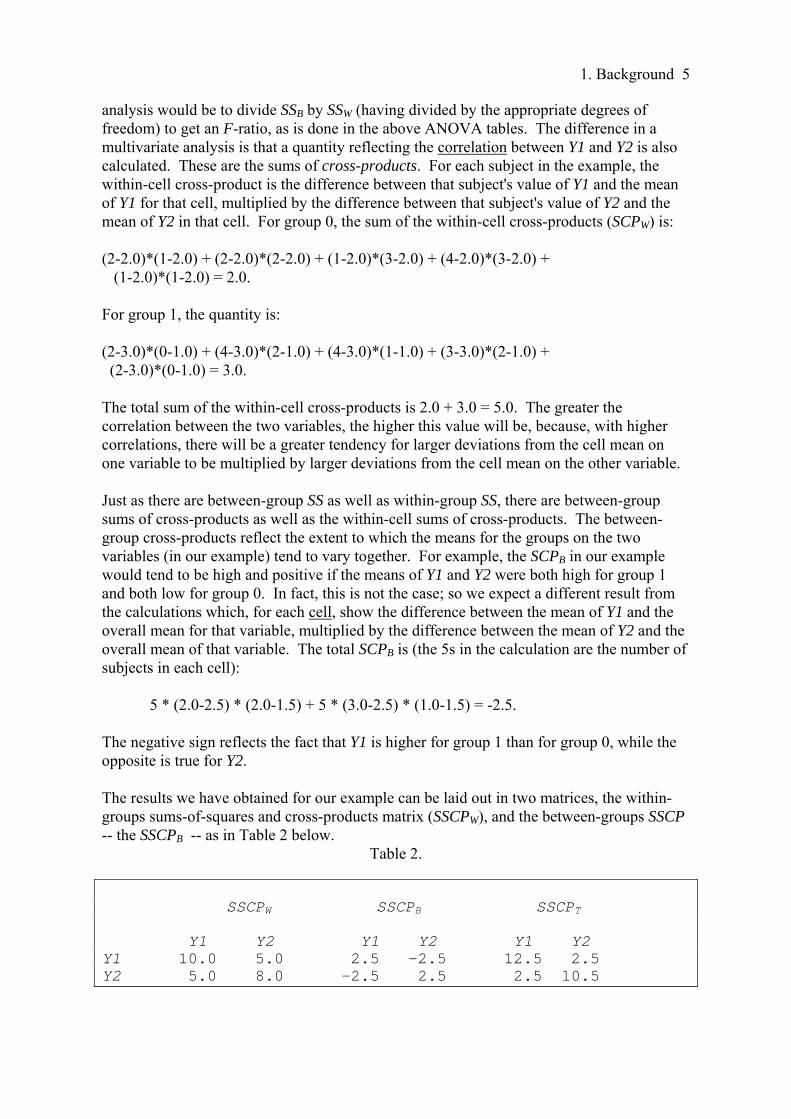
analysis would be to divide SSB by SSW (having divided by the appropriate degrees of freedom) to get an F-ratio, as is done in the above ANOVA tables. The difference in a multivariate analysis is that a quantity reflecting the correlation between Y1 and Y2 is also calculated. These are the sums of cross-products. For each subject in the example, the within-cell cross-product is the difference between that subject's value of Y1 and the mean of Y1 for that cell, multiplied by the difference between that subject's value of Y2 and the mean of Y2 in that cell. For group 0, the sum of the within-cell cross-products (SCPW) is: (2-2.0)*(1-2.0) + (2-2.0)*(2-2.0) + (1-2.0)*(3-2.0) + (4-2.0)*(3-2.0) + (1-2.0)*(1-2.0) = 2.0. For group 1, the quantity is: (2-3.0)*(0-1.0) + (4-3.0)*(2-1.0) + (4-3.0)*(1-1.0) + (3-3.0)*(2-1.0) + (2-3.0)*(0-1.0) = 3.0. The total sum of the within-cell cross-products is 2.0 + 3.0 = 5.0. The greater the correlation between the two variables, the higher this value will be, because, with higher correlations, there will be a greater tendency for larger deviations from the cell mean on one variable to be multiplied by larger deviations from the cell mean on the other variable. Just as there are between-group SS as well as within-group SS, there are between-group sums of cross-products as well as the within-cell sums of cross-products. The between-group cross-products reflect the extent to which the means for the groups on the two variables (in our example) tend to vary together. For example, the SCPB in our example would tend to be high and positive if the means of Y1 and Y2 were both high for group 1 and both low for group 0. In fact, this is not the case; so we expect a different result from the calculations which, for each cell, show the difference between the mean of Y1 and the overall mean for that variable, multiplied by the difference between the mean of Y2 and the overall mean of that variable. The total SCPB is (the 5s in the calculation are the number of subjects in each cell): 5 * (2.0-2.5) * (2.0-1.5) + 5 * (3.0-2.5) * (1.0-1.5) = -2.5. The negative sign reflects the fact that Y1 is higher for group 1 than for group 0, while the opposite is true for Y2. The results we have obtained for our example can be laid out in two matrices, the within-groups sums-of-squares and cross-products matrix (SSCPW), and the between-groups SSCP -- the SSCPB -- as in Table 2 below.
Table 2. SSCPW SSCPB SSCPT Y1 Y2 Y1 Y2 Y1 Y2 Y1 10.0 5.0 2.5 -2.5 12.5 2.5 Y2 5.0 8.0 -2.5 2.5 2.5 10.5
1. Background 6
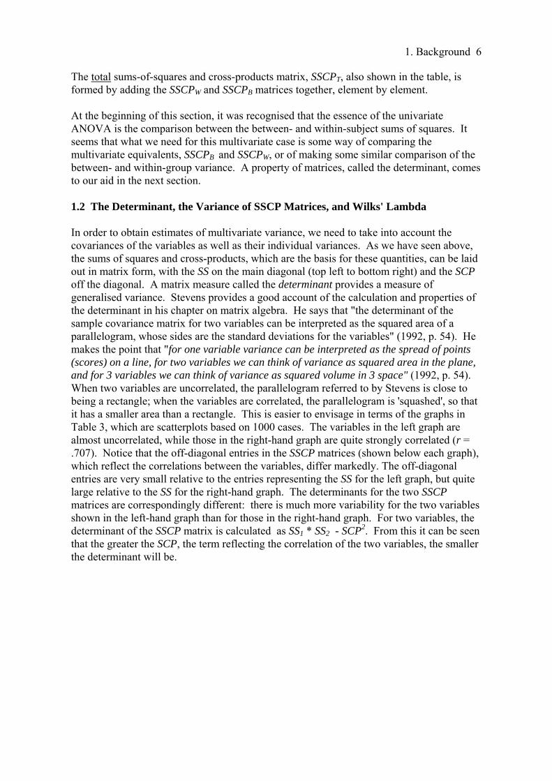
The total sums-of-squares and cross-products matrix, SSCPT, also shown in the table, is formed by adding the SSCPW and SSCPB matrices together, element by element. At the beginning of this section, it was recognised that the essence of the univariate ANOVA is the comparison between the between- and within-subject sums of squares. It seems that what we need for this multivariate case is some way of comparing the multivariate equivalents, SSCPB and SSCPW, or of making some similar comparison of the between- and within-group variance. A property of matrices, called the determinant, comes to our aid in the next section. 1.2 The Determinant, the Variance of SSCP Matrices, and Wilks' Lambda In order to obtain estimates of multivariate variance, we need to take into account the covariances of the variables as well as their individual variances. As we have seen above, the sums of squares and cross-products, which are the basis for these quantities, can be laid out in matrix form, with the SS on the main diagonal (top left to bottom right) and the SCP off the diagonal. A matrix measure called the determinant provides a measure of generalised variance. Stevens provides a good account of the calculation and properties of the determinant in his chapter on matrix algebra. He says that "the determinant of the sample covariance matrix for two variables can be interpreted as the squared area of a parallelogram, whose sides are the standard deviations for the variables" (1992, p. 54). He makes the point that "for one variable variance can be interpreted as the spread of points (scores) on a line, for two variables we can think of variance as squared area in the plane, and for 3 variables we can think of variance as squared volume in 3 space" (1992, p. 54). When two variables are uncorrelated, the parallelogram referred to by Stevens is close to being a rectangle; when the variables are correlated, the parallelogram is 'squashed', so that it has a smaller area than a rectangle. This is easier to envisage in terms of the graphs in Table 3, which are scatterplots based on 1000 cases. The variables in the left graph are almost uncorrelated, while those in the right-hand graph are quite strongly correlated (r = .707). Notice that the off-diagonal entries in the SSCP matrices (shown below each graph), which reflect the correlations between the variables, differ markedly. The off-diagonal entries are very small relative to the entries representing the SS for the left graph, but quite large relative to the SS for the right-hand graph. The determinants for the two SSCP matrices are correspondingly different: there is much more variability for the two variables shown in the left-hand graph than for those in the right-hand graph. For two variables, the determinant of the SSCP matrix is calculated as SS1 * SS2 - SCP2. From this it can be seen that the greater the SCP, the term reflecting the correlation of the two variables, the smaller the determinant will be.

1. Background 7
Table 3.
r = -.009 r = .717 SSCP matrix SSCP matrix 975.9 -9.3 998.9 743.2 -9.3 999.9 743.2 1074.8 Determinant = 975,662.5 Determinant = 521,270.7 As a measure of the variance of matrices, the determinant makes it possible to compare the various types of SSCP matrix, and in fact it is the basis for the most commonly-used multivariate statistic, Wilks' Lambda. If we use W to stand for the within-cells SSCP matrix (sometimes called the error SSCP, or E), like the one at the left-hand end of Table 2; B to stand for the between-groups SSCP (sometimes called the hypothesis SSCP, or H), like the one in the middle of Table 2; and T to stand for the total SSCP (B + W), like the one at the right-hand end of Table 2, Wilks' Lambda, , is equal to
|W | -------
|T |
where |W | is the determinant of W, and | T | is the determinant of T. As is evident from the formula, shows the proportion of the total variance of the dependent variables which is not due to differences between the groups. Thus, the smaller the value of , the larger the effect of group. Going back to the example for which we worked out the SSCP matrices above (Table 2), the determinants of W and T are (10 * 8 - 52) = 55 and (12.5 * 10.5 - 2.52) = 125 respectively. is therefore equal to 55/125 = .44. This figure means that 44% of the variance of Y1 and Y2 is not accounted for by the grouping variable, and that 56% is. Tests of the statistical significance of are described by Stevens (1992, p. 192) and Tacq (1997, p. 351). The distribution of is complex, and the probabilities which SPSS and other programs print out are usually based on approximations, although in some cases (when the number of groups is 2, for example) the probabilities are exact. The result for this example is that Wilks' Lambda = .44, F(2,7) = 4.46, p = .057.
1. Background 8
We now have a way of testing the significance of the difference between groups when there are multiple dependent variables, and it is a way which is based on an extension of the method used in univariate analyses. We can see that the method used for MANOVA takes into account the correlations between the dependent variables as well as the differences between their means. It is also possible to see the circumstances under which a multivariate analysis is most likely to show differences between groups. Smaller values of Wilks' Lambda correspond to larger differences between groups, and smaller values of Lambda arise from relatively smaller values of |W |, the determinant of SSCPW. One of the things which contributes to a smaller determinant |W | is a high within-cell correlation between dependent variables. The size of the ratio |W|/| T | will therefore be smallest when the dependent variables are highly correlated and, correspondingly, when the between-group differences are not highly correlated. The latter situation will lead to higher values of | T|. The between-group differences will tend to be uncorrelated if the pattern of the means differs over groups; if, for example, group 0 is higher than group 1 on Y1, but lower than group 1 on Y2. An example discussed later will make this clearer. It is possible to think that a multivariate analysis could provide information beyond the knowledge that there is a significant difference between groups; for example, how does each of the different dependent variables contribute to differentiating between the groups? Would we be as well off (in terms of distinguishing between groups) with just one or two of the variables, rather than a greater number? As it turns out, there's another way of approaching MANOVA, which answers these questions, and which leads us back to Wilks' Lambda, calculated by a different but equivalent method. 1.3 Differentiating Between Groups with the Discriminant Function - A Weighted Composite Variable Another approach to the 'problem' of having more than one dependent variable is to combine the variables to make a composite variable, and then to carry out a simple univariate analysis on the composite variable. The big question then is how to combine the variables. The simplest way of combining a number of variables is simply to add them together. For instance, say we have two dependent variables which are the results for a number of subjects on two ability scales, maths and language. We could create a composite variable from these variables by using the SPSS command compute score = maths + language. This is equivalent to the command compute score = 1 * maths + 1 * language. where the 1s are weights, in this case both the same value. The variable score is called a weighted composite. In MANOVA, the analysis rests on creating one or more weighted composite variables (called discriminant functions or canonical variates) from the dependent variables. Suppose in this example that there are two groups of subjects. The trick that MANOVA performs is to choose weights which produce a composite which is as different as possible for the two groups. To continue with our maths and language example, say there are two groups, numbered 1 and 2, and two dependent variables, maths
1. Background 9
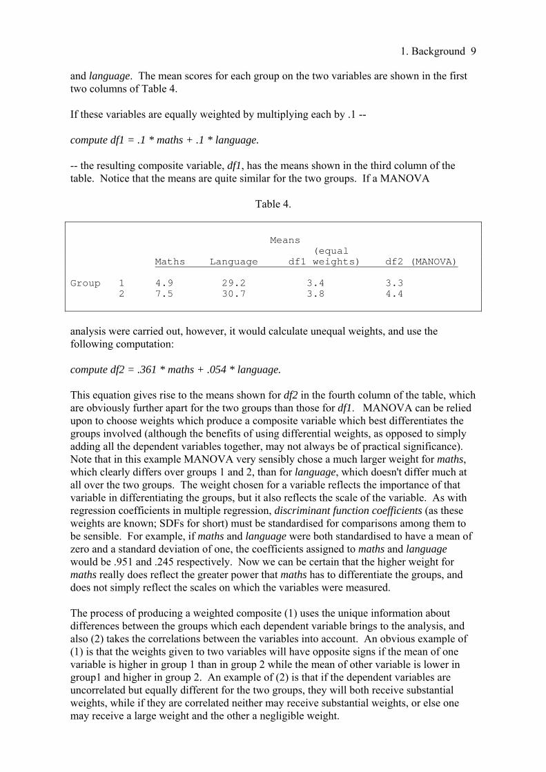
and language. The mean scores for each group on the two variables are shown in the first two columns of Table 4. If these variables are equally weighted by multiplying each by .1 -- compute df1 = .1 * maths + .1 * language. -- the resulting composite variable, df1, has the means shown in the third column of the table. Notice that the means are quite similar for the two groups. If a MANOVA
Table 4.
Means (equal Maths Language df1 weights) df2 (MANOVA) Group 1 4.9 29.2 3.4 3.3 2 7.5 30.7 3.8 4.4
analysis were carried out, however, it would calculate unequal weights, and use the following computation: compute df2 = .361 * maths + .054 * language. This equation gives rise to the means shown for df2 in the fourth column of the table, which are obviously further apart for the two groups than those for df1. MANOVA can be relied upon to choose weights which produce a composite variable which best differentiates the groups involved (although the benefits of using differential weights, as opposed to simply adding all the dependent variables together, may not always be of practical significance). Note that in this example MANOVA very sensibly chose a much larger weight for maths, which clearly differs over groups 1 and 2, than for language, which doesn't differ much at all over the two groups. The weight chosen for a variable reflects the importance of that variable in differentiating the groups, but it also reflects the scale of the variable. As with regression coefficients in multiple regression, discriminant function coefficients (as these weights are known; SDFs for short) must be standardised for comparisons among them to be sensible. For example, if maths and language were both standardised to have a mean of zero and a standard deviation of one, the coefficients assigned to maths and language would be .951 and .245 respectively. Now we can be certain that the higher weight for maths really does reflect the greater power that maths has to differentiate the groups, and does not simply reflect the scales on which the variables were measured. The process of producing a weighted composite (1) uses the unique information about differences between the groups which each dependent variable brings to the analysis, and also (2) takes the correlations between the variables into account. An obvious example of (1) is that the weights given to two variables will have opposite signs if the mean of one variable is higher in group 1 than in group 2 while the mean of other variable is lower in group1 and higher in group 2. An example of (2) is that if the dependent variables are uncorrelated but equally different for the two groups, they will both receive substantial weights, while if they are correlated neither may receive substantial weights, or else one may receive a large weight and the other a negligible weight.
1. Background 10
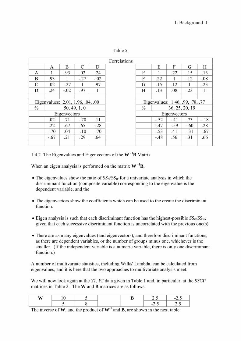
1.4 Choosing the Weights: Eigenvalues and Eigenvectors No attempt will be made here to give a detailed derivation of the method used by MANOVA to calculate optimal weights for the composite variable or discriminant function. Tacq (1997) gives a good description (pp. 242-246); however, even a lofty general view of the process requires an acquaintance with the mathematical concepts of the eigenvalue and eigenvector, and it's worth a bit of effort, because they crop up as the basis of a number of multivariate techniques, apart from MANOVA (e.g., principal components analysis). Before talking about eigen analysis, we should renew acquaintance with the SSCPW and SSCPB matrices, such as those shown in Table 2. Here, they'll be referred to as matrices W and B. The matrix equivalent of SSB/SSW is W -1B, where W -1 is the inverse of W . The inverse of a matrix is the equivalent of the reciprocal of a single number, e.g., 1/x. (For further information about the inverse, see Tacq (1997), pp. 396-397.) 1.4.1 The Eigenvalues and Eigenvectors of a Correlation Matrix The eigenvalues of a matrix (which are single numbers) represent some optimum point to do with the contents of that matrix; for example, the first eigenvalue of a correlation matrix for variables a, b, c and d shows the maximum amount of variance of the variables a, b, c and d that can be represented by a single composite variable. As an example, take the two correlation matrices in Table 5. In the first, there are high correlations between a and b and between c and d. In the second, the correlations between e, f, g and h are uniformly low. The first eigenvalue for the a, b, c, d table, 2.01, shows that a first optimal composite variable would account for a substantial part of the variance of a, b, c and d. Because there are four variables, the total variance is 4.0, so that the first composite variable would account for (2.01/4) * 100 = 50% of the variance. The second eigenvalue, 1.96, shows that a second composite variable, uncorrelated with the first, would account for a further 49% of the variance of a, b, c and d; so the four variables could be very well represented by two composite variables. The eigenvalues for the second correlation matrix, on the other hand, are all fairly small, reflecting the fact that e, f, g and h are not highly correlated, so that as many composite variables as there are variables would be needed to represent a substantial amount of the variance of e, f, g and h. As well as producing eigenvalues, an eigen analysis produces eigenvectors, one corresponding to each eigenvalue. When the analysis is of correlation matrices like those in Table 5, eigenvectors show the weights by which each variable should be multiplied in order to produce the optimal composite variable corresponding to the eigenvalue; for example, the eigenvector corresponding to the first eigenvalue for the a, b, c, d correlation matrix has high values for variables c and d, and lower values for variables a and b. The second eigenvector has high values for a and b, and lower values for c and d. The values in the eigenvectors for the correlation matrix for e, f, g and h are fairly uniform, reflecting the general lack of association between the variables.
1. Background 11
Table 5.
Correlations A B C D E F G H
A 1 .93 .02 .24 E 1 .22 .15 .13 B .93 1 -.27 -.02 F .22 1 .12 .08 C .02 -.27 1 .97 G .15 .12 1 .23 D .24 -.02 .97 1 H .13 .08 .23 1
Eigenvalues: 2.01, 1.96, .04, .00 Eigenvalues: 1.46, .99, .78, .77 % 50, 49, 1, 0 % 36, 25, 20, 19
Eigenvectors Eigenvectors .02 .71 -.70 .11 -.52 -.41 .73 -.18 .22 .67 .65 -.28 -.47 -.59 -.60 .28 -.70 .04 -.10 -.70 -.53 .41 -.31 -.67 -.67 .21 .29 .64 -.48 .56 .31 .66
1.4.2 The Eigenvalues and Eigenvectors of the W -1B Matrix When an eigen analysis is performed on the matrix W -1B, The eigenvalues show the ratio of SSB/SSW for a univariate analysis in which the
discriminant function (composite variable) corresponding to the eigenvalue is the dependent variable, and the
The eigenvectors show the coefficients which can be used to the create the discriminant function.
Eigen analysis is such that each discriminant function has the highest-possible SSB/SSW, given that each successive discriminant function is uncorrelated with the previous one(s).
There are as many eigenvalues (and eigenvectors), and therefore discriminant functions, as there are dependent variables, or the number of groups minus one, whichever is the smaller. (If the independent variable is a numeric variable, there is only one discriminant function.)
A number of multivariate statistics, including Wilks' Lambda, can be calculated from eigenvalues, and it is here that the two approaches to multivariate analysis meet. We will now look again at the Y1, Y2 data given in Table 1 and, in particular, at the SSCP matrices in Table 2. The W and B matrices are as follows:
10 5 2.5 -2.5 W 5 8
B -2.5 2.5
The inverse of W, and the product of W-1 and B, are shown in the next table:
1. Background 12
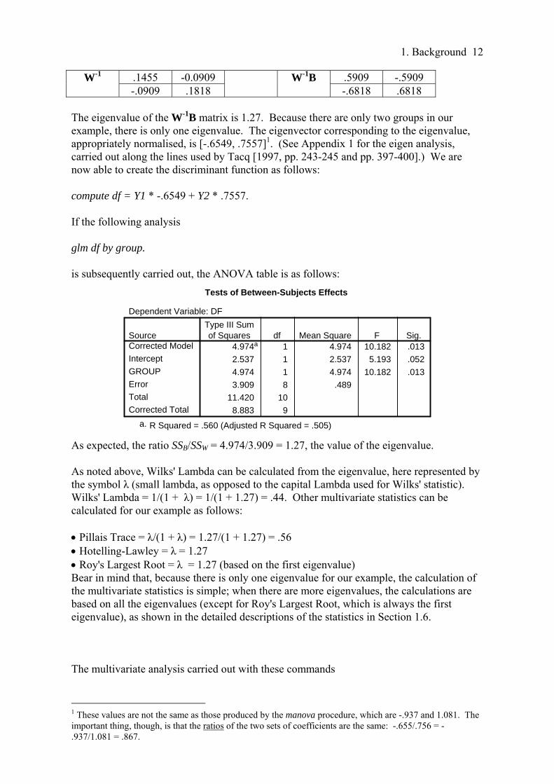
.1455 -0.0909 .5909 -.5909 W-1 -.0909 .1818
W-1B -.6818 .6818
The eigenvalue of the W-1B matrix is 1.27. Because there are only two groups in our example, there is only one eigenvalue. The eigenvector corresponding to the eigenvalue, appropriately normalised, is [-.6549, .7557]1. (See Appendix 1 for the eigen analysis, carried out along the lines used by Tacq [1997, pp. 243-245 and pp. 397-400].) We are now able to create the discriminant function as follows: compute df = Y1 * -.6549 + Y2 * .7557. If the following analysis glm df by group. is subsequently carried out, the ANOVA table is as follows:
Tests of Between-Subjects Effects
Dependent Variable: DF
4.974a 1 4.974 10.182 .013
2.537 1 2.537 5.193 .052
4.974 1 4.974 10.182 .013
3.909 8 .489
11.420 10
8.883 9
SourceCorrected Model
Intercept
GROUP
Error
Total
Corrected Total
Type III Sumof Squares df Mean Square F Sig.
R Squared = .560 (Adjusted R Squared = .505)a.
As expected, the ratio SSB/SSW = 4.974/3.909 = 1.27, the value of the eigenvalue. As noted above, Wilks' Lambda can be calculated from the eigenvalue, here represented by the symbol λ (small lambda, as opposed to the capital Lambda used for Wilks' statistic). Wilks' Lambda = 1/(1 + λ) = 1/(1 + 1.27) = .44. Other multivariate statistics can be calculated for our example as follows: Pillais Trace = λ/(1 + λ) = 1.27/(1 + 1.27) = .56 Hotelling-Lawley = λ = 1.27 Roy's Largest Root = λ = 1.27 (based on the first eigenvalue) Bear in mind that, because there is only one eigenvalue for our example, the calculation of the multivariate statistics is simple; when there are more eigenvalues, the calculations are based on all the eigenvalues (except for Roy's Largest Root, which is always the first eigenvalue), as shown in the detailed descriptions of the statistics in Section 1.6. The multivariate analysis carried out with these commands
1 These values are not the same as those produced by the manova procedure, which are -.937 and 1.081. The important thing, though, is that the ratios of the two sets of coefficients are the same: -.655/.756 = -.937/1.081 = .867.
1. Background 13
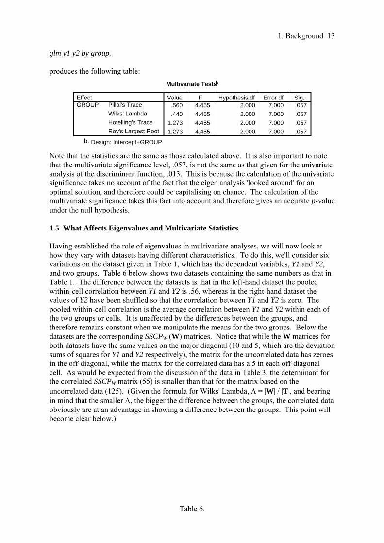
glm y1 y2 by group. produces the following table:
Multivariate Testsb
.560 4.455 2.000 7.000 .057
.440 4.455 2.000 7.000 .057
1.273 4.455 2.000 7.000 .057
1.273 4.455 2.000 7.000 .057
Pillai's Trace
Wilks' Lambda
Hotelling's Trace
Roy's Largest Root
EffectGROUP
Value F Hypothesis df Error df Sig.
Design: Intercept+GROUPb.
Note that the statistics are the same as those calculated above. It is also important to note that the multivariate significance level, .057, is not the same as that given for the univariate analysis of the discriminant function, .013. This is because the calculation of the univariate significance takes no account of the fact that the eigen analysis 'looked around' for an optimal solution, and therefore could be capitalising on chance. The calculation of the multivariate significance takes this fact into account and therefore gives an accurate p-value under the null hypothesis. 1.5 What Affects Eigenvalues and Multivariate Statistics Having established the role of eigenvalues in multivariate analyses, we will now look at how they vary with datasets having different characteristics. To do this, we'll consider six variations on the dataset given in Table 1, which has the dependent variables, Y1 and Y2, and two groups. Table 6 below shows two datasets containing the same numbers as that in Table 1. The difference between the datasets is that in the left-hand dataset the pooled within-cell correlation between Y1 and Y2 is .56, whereas in the right-hand dataset the values of Y2 have been shuffled so that the correlation between Y1 and Y2 is zero. The pooled within-cell correlation is the average correlation between Y1 and Y2 within each of the two groups or cells. It is unaffected by the differences between the groups, and therefore remains constant when we manipulate the means for the two groups. Below the datasets are the corresponding SSCPW (W) matrices. Notice that while the W matrices for both datasets have the same values on the major diagonal (10 and 5, which are the deviation sums of squares for Y1 and Y2 respectively), the matrix for the uncorrelated data has zeroes in the off-diagonal, while the matrix for the correlated data has a 5 in each off-diagonal cell. As would be expected from the discussion of the data in Table 3, the determinant for the correlated SSCPW matrix (55) is smaller than that for the matrix based on the uncorrelated data (125). (Given the formula for Wilks' Lambda, = |W| / |T|, and bearing in mind that the smaller , the bigger the difference between the groups, the correlated data obviously are at an advantage in showing a difference between the groups. This point will become clear below.)
Table 6.

1. Background 14
Correlated Uncorrelated
Y1 Y2 GROUP Y1 Y2
2 1 0 2 1 2 2 0 2 3 1 3 0 1 1 4 3 0 4 2 1 1 0 1 3 2 0 1 2 2 4 2 1 4 2 4 1 1 4 0 3 2 1 3 1 2 0 1 2 0
r = .56 r = 0.00
SSCPW SSCPW
10 5 10 0 5 8 0 8 |W| = 55 |W| = 125
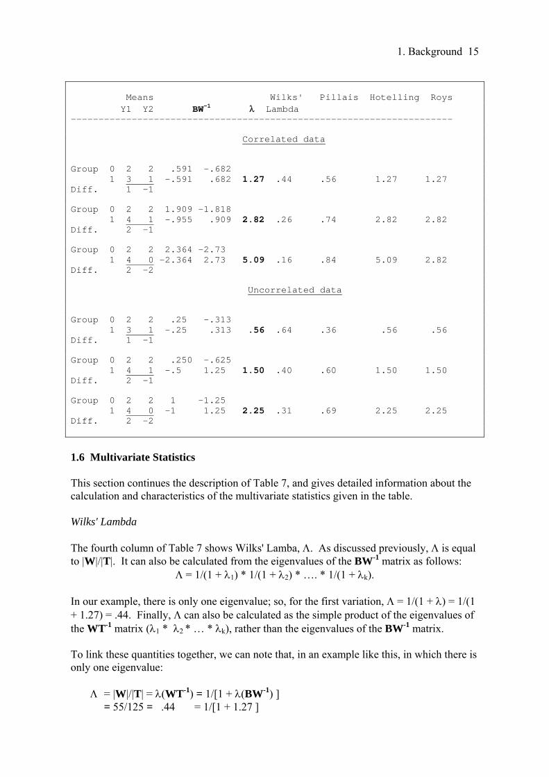
Table 7 shows the six variations of the data in Table 6. The first three examples are based on the correlated data. The first variation is simply based on the means of the data in Table 6. The second variation was produced by adding one to Y1 for all the cases in Group 1 (thus making the differences between the groups larger), while the third variation was produced by adding one to Y1 and subtracting one from Y2 for all the subjects in Group 1 (making the differences between the groups larger still). The fourth, fifth and sixth examples are for the uncorrelated data. The variations in means are the same as those for the correlated data. Working across the table, the first column shows the means of Y1 and Y2 for each group, and the difference between the means for the two groups. The next column shows the BW-
1 matrix for each variation. For both the correlated and uncorrelated data, the values in the matrix are greater with greater differences between the means. Also, for each variation in the means, the values are greater for the correlated data than for the uncorrelated data. The entries on the major diagonal of the BW-1 matrix are directly related to the eigenvalue, , which is shown in the next column. In fact, is equal to the sum of the entries on the diagonal. (If there were more than one eigenvalue, the sum of the diagonal BW-1
entries would equal the sum of the eigenvalues.)
Table 7.
1. Background 15
Means Wilks' Pillais Hotelling Roys Y1 Y2 BW-1 Lambda --------------------------------------------------------------------- Correlated data
Group 0 2 2 .591 -.682 1 3 1 -.591 .682 1.27 .44 .56 1.27 1.27 Diff. 1 -1 Group 0 2 2 1.909 -1.818 1 4 1 -.955 .909 2.82 .26 .74 2.82 2.82 Diff. 2 -1 Group 0 2 2 2.364 -2.73 1 4 0 -2.364 2.73 5.09 .16 .84 5.09 2.82 Diff. 2 -2 Uncorrelated data
Group 0 2 2 .25 -.313 1 3 1 -.25 .313 .56 .64 .36 .56 .56 Diff. 1 -1 Group 0 2 2 .250 -.625 1 4 1 -.5 1.25 1.50 .40 .60 1.50 1.50 Diff. 2 -1 Group 0 2 2 1 -1.25 1 4 0 -1 1.25 2.25 .31 .69 2.25 2.25 Diff. 2 -2
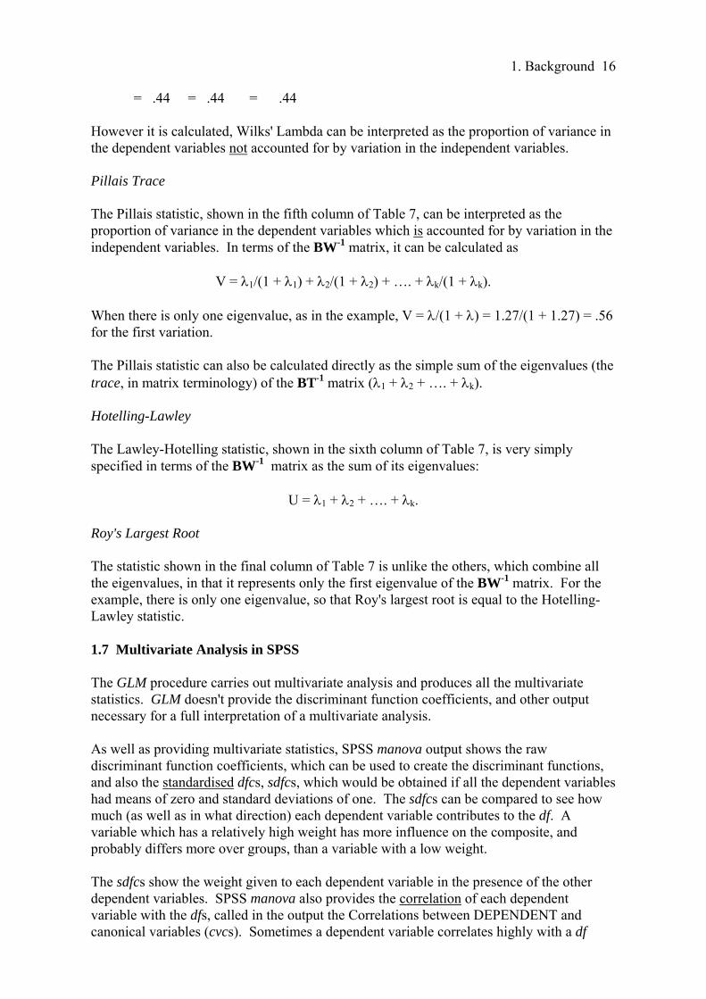
1.6 Multivariate Statistics This section continues the description of Table 7, and gives detailed information about the calculation and characteristics of the multivariate statistics given in the table. Wilks' Lambda The fourth column of Table 7 shows Wilks' Lamba, . As discussed previously, is equal to |W|/|T|. It can also be calculated from the eigenvalues of the BW-1 matrix as follows:
= 1/(1 + 1) * 1/(1 + 2) * …. * 1/(1 + k). In our example, there is only one eigenvalue; so, for the first variation, = 1/(1 + ) = 1/(1 + 1.27) = .44. Finally, can also be calculated as the simple product of the eigenvalues of the WT-1 matrix (1 * 2 * … * k), rather than the eigenvalues of the BW-1 matrix. To link these quantities together, we can note that, in an example like this, in which there is only one eigenvalue: = |W|/|T| = (WT-1) = 1/[1 + (BW-1) ] = 55/125 = .44 = 1/[1 + 1.27 ]
1. Background 16
= .44 = .44 = .44 However it is calculated, Wilks' Lambda can be interpreted as the proportion of variance in the dependent variables not accounted for by variation in the independent variables. Pillais Trace The Pillais statistic, shown in the fifth column of Table 7, can be interpreted as the proportion of variance in the dependent variables which is accounted for by variation in the independent variables. In terms of the BW-1 matrix, it can be calculated as
V = 1/(1 + 1) + 2/(1 + 2) + …. + k/(1 + k). When there is only one eigenvalue, as in the example, V = /(1 + ) = 1.27/(1 + 1.27) = .56 for the first variation. The Pillais statistic can also be calculated directly as the simple sum of the eigenvalues (the trace, in matrix terminology) of the BT-1 matrix (1 + 2 + …. + k). Hotelling-Lawley The Lawley-Hotelling statistic, shown in the sixth column of Table 7, is very simply specified in terms of the BW-1 matrix as the sum of its eigenvalues:
U = 1 + 2 + …. + k. Roy's Largest Root The statistic shown in the final column of Table 7 is unlike the others, which combine all the eigenvalues, in that it represents only the first eigenvalue of the BW-1 matrix. For the example, there is only one eigenvalue, so that Roy's largest root is equal to the Hotelling-Lawley statistic. 1.7 Multivariate Analysis in SPSS The GLM procedure carries out multivariate analysis and produces all the multivariate statistics. GLM doesn't provide the discriminant function coefficients, and other output necessary for a full interpretation of a multivariate analysis. As well as providing multivariate statistics, SPSS manova output shows the raw discriminant function coefficients, which can be used to create the discriminant functions, and also the standardised dfcs, sdfcs, which would be obtained if all the dependent variables had means of zero and standard deviations of one. The sdfcs can be compared to see how much (as well as in what direction) each dependent variable contributes to the df. A variable which has a relatively high weight has more influence on the composite, and probably differs more over groups, than a variable with a low weight. The sdfcs show the weight given to each dependent variable in the presence of the other dependent variables. SPSS manova also provides the correlation of each dependent variable with the dfs, called in the output the Correlations between DEPENDENT and canonical variables (cvcs). Sometimes a dependent variable correlates highly with a df
1. Background 17
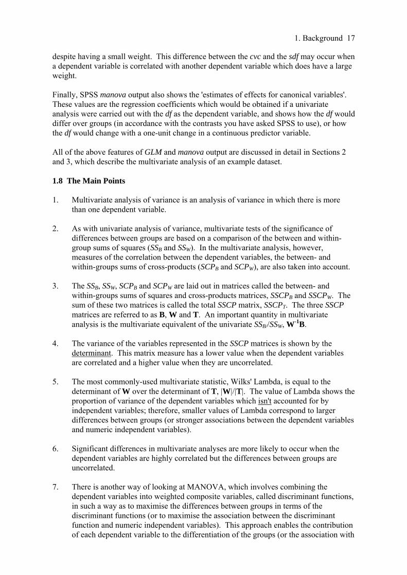
despite having a small weight. This difference between the cvc and the sdf may occur when a dependent variable is correlated with another dependent variable which does have a large weight. Finally, SPSS manova output also shows the 'estimates of effects for canonical variables'. These values are the regression coefficients which would be obtained if a univariate analysis were carried out with the df as the dependent variable, and shows how the df would differ over groups (in accordance with the contrasts you have asked SPSS to use), or how the df would change with a one-unit change in a continuous predictor variable. All of the above features of GLM and manova output are discussed in detail in Sections 2 and 3, which describe the multivariate analysis of an example dataset. 1.8 The Main Points
1. Multivariate analysis of variance is an analysis of variance in which there is more
than one dependent variable.
2. As with univariate analysis of variance, multivariate tests of the significance of differences between groups are based on a comparison of the between and within-group sums of squares (SSB and SSW). In the multivariate analysis, however, measures of the correlation between the dependent variables, the between- and within-groups sums of cross-products (SCPB and SCPW), are also taken into account.
3. The SSB, SSW, SCPB and SCPW are laid out in matrices called the between- and within-groups sums of squares and cross-products matrices, SSCPB and SSCPW. The sum of these two matrices is called the total SSCP matrix, SSCPT. The three SSCP matrices are referred to as B, W and T. An important quantity in multivariate analysis is the multivariate equivalent of the univariate SSB//SSW, W-1B.
4. The variance of the variables represented in the SSCP matrices is shown by the determinant. This matrix measure has a lower value when the dependent variables are correlated and a higher value when they are uncorrelated.
5. The most commonly-used multivariate statistic, Wilks' Lambda, is equal to the determinant of W over the determinant of T, |W|/|T|. The value of Lambda shows the proportion of variance of the dependent variables which isn't accounted for by independent variables; therefore, smaller values of Lambda correspond to larger differences between groups (or stronger associations between the dependent variables and numeric independent variables).
6. Significant differences in multivariate analyses are more likely to occur when the dependent variables are highly correlated but the differences between groups are uncorrelated.
7. There is another way of looking at MANOVA, which involves combining the dependent variables into weighted composite variables, called discriminant functions, in such a way as to maximise the differences between groups in terms of the discriminant functions (or to maximise the association between the discriminant function and numeric independent variables). This approach enables the contribution of each dependent variable to the differentiation of the groups (or the association with
1. Background 18
the numeric variable) to be assessed. It also leads back to Wilks' Lambda, and its calculation by a different but equivalent method to that described above.
8. The weights used to create each discriminant function (called the discriminant function coefficients, dfc) are chosen so as to maximise the difference of the df over groups (or to maximise the correlation of the df with a continuous predictor variable).
9. More specifically, the weights are chosen to maximise the ratio of the between-groups sums of squares (SS) to the within-groups sums of squares for the df.
10. A mathematical process called eigen analysis, when applied to the matrix W-1B, gives
rise to eigenvalues and eigenvectors. An eigenvalue shows the ratio of SSB to SSW for a univariate analysis with the discriminant function as the dependent variable.
11. An eigenvector contains the coefficients which, if appropriately normalised, and applied to the dependent variables, will produce a discriminant function which best differentiates the groups (or correlates most highly with a numeric independent variable). No other combination of coefficients can produce a discriminant function which better differentiates the groups (or correlates more highly with a numeric independent variable).
12. There are as many eigenvalues (each corresponding to a discriminant function) as there are dependent variables, or the number of groups minus one, whichever is the smaller (there is only one discriminant function for each numeric independent variable). Each successive discriminant function is uncorrelated with the previous one(s).
13. It turns out that Wilks' Lambda, and other multivariate statistics, can be derived from the eigenvalues of the W-1B matrix, and from the eigenvalues of other matrices, such as WT-1 and BW-1.
14. While the SPSS GLM procedure provides multivariate statistics, it is necessary to use the manova procedure to obtain discriminant function coefficients and other information necessary for the full interpretation of a multivariate analysis.
2. Multivariate Analysis with GLM 19
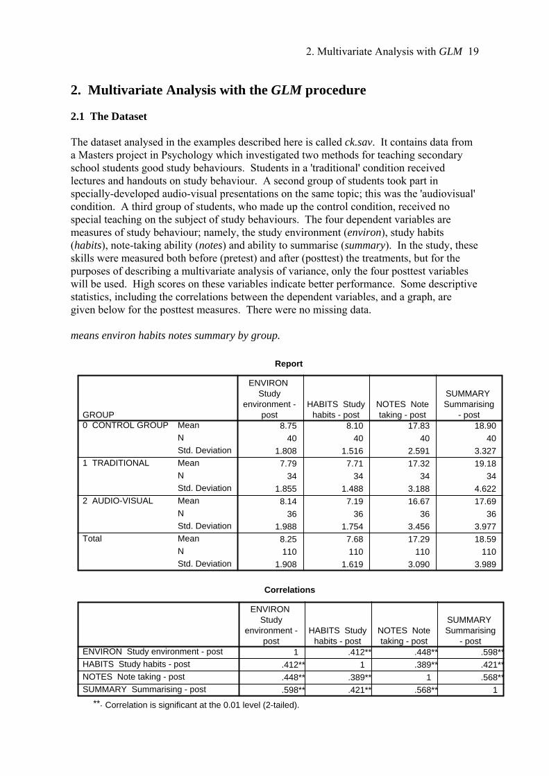
2. Multivariate Analysis with the GLM procedure 2.1 The Dataset The dataset analysed in the examples described here is called ck.sav. It contains data from a Masters project in Psychology which investigated two methods for teaching secondary school students good study behaviours. Students in a 'traditional' condition received lectures and handouts on study behaviour. A second group of students took part in specially-developed audio-visual presentations on the same topic; this was the 'audiovisual' condition. A third group of students, who made up the control condition, received no special teaching on the subject of study behaviours. The four dependent variables are measures of study behaviour; namely, the study environment (environ), study habits (habits), note-taking ability (notes) and ability to summarise (summary). In the study, these skills were measured both before (pretest) and after (posttest) the treatments, but for the purposes of describing a multivariate analysis of variance, only the four posttest variables will be used. High scores on these variables indicate better performance. Some descriptive statistics, including the correlations between the dependent variables, and a graph, are given below for the posttest measures. There were no missing data. means environ habits notes summary by group.
Report
8.75 8.10 17.83 18.90
40 40 40 40
1.808 1.516 2.591 3.327
7.79 7.71 17.32 19.18
34 34 34 34
1.855 1.488 3.188 4.622
8.14 7.19 16.67 17.69
36 36 36 36
1.988 1.754 3.456 3.977
8.25 7.68 17.29 18.59
110 110 110 110
1.908 1.619 3.090 3.989
Mean
N
Std. Deviation
Mean
N
Std. Deviation
Mean
N
Std. Deviation
Mean
N
Std. Deviation
GROUP0 CONTROL GROUP
1 TRADITIONAL
2 AUDIO-VISUAL
Total
ENVIRON Study
environment -post
HABITS Studyhabits - post
NOTES Notetaking - post
SUMMARY Summarising
- post
Correlations
1 .412** .448** .598**
.412** 1 .389** .421**
.448** .389** 1 .568**
.598** .421** .568** 1
ENVIRON Study environment - post
HABITS Study habits - post
NOTES Note taking - post
SUMMARY Summarising - post
ENVIRON Study
environment -post
HABITS Studyhabits - post
NOTES Notetaking - post
SUMMARY Summarising
- post
Correlation is significant at the 0.01 level (2-tailed).**.
2. Multivariate Analysis with GLM 20
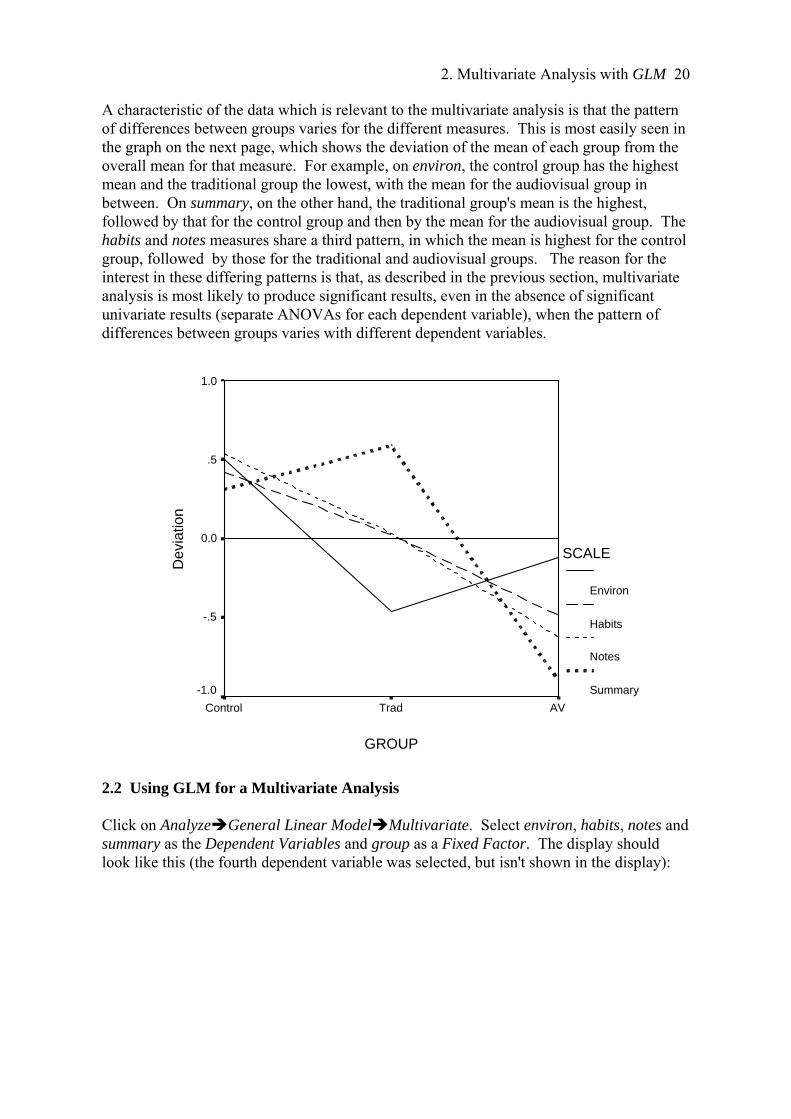
A characteristic of the data which is relevant to the multivariate analysis is that the pattern of differences between groups varies for the different measures. This is most easily seen in the graph on the next page, which shows the deviation of the mean of each group from the overall mean for that measure. For example, on environ, the control group has the highest mean and the traditional group the lowest, with the mean for the audiovisual group in between. On summary, on the other hand, the traditional group's mean is the highest, followed by that for the control group and then by the mean for the audiovisual group. The habits and notes measures share a third pattern, in which the mean is highest for the control group, followed by those for the traditional and audiovisual groups. The reason for the interest in these differing patterns is that, as described in the previous section, multivariate analysis is most likely to produce significant results, even in the absence of significant univariate results (separate ANOVAs for each dependent variable), when the pattern of differences between groups varies with different dependent variables.
GROUP
AVTradControl
Dev
iatio
n
1.0
.5
0.0
-.5
-1.0
SCALE
Environ
Habits
Notes
Summary
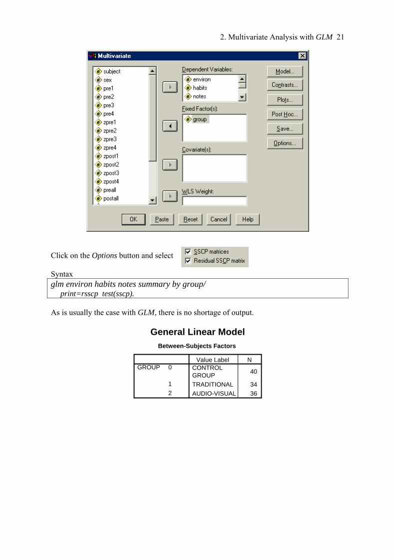
2.2 Using GLM for a Multivariate Analysis Click on AnalyzeGeneral Linear ModelMultivariate. Select environ, habits, notes and summary as the Dependent Variables and group as a Fixed Factor. The display should look like this (the fourth dependent variable was selected, but isn't shown in the display):
2. Multivariate Analysis with GLM 21
Click on the Options button and select Syntax glm environ habits notes summary by group/ print=rsscp test(sscp). As is usually the case with GLM, there is no shortage of output.
General Linear Model
Between-Subjects Factors
CONTROLGROUP
40
TRADITIONAL 34
AUDIO-VISUAL 36
0
1
2
GROUPValue Label N
2. Multivariate Analysis with GLM 22
Multivariate Testsc
.977 1125.635a 4.000 104.000 .000
.023 1125.635a 4.000 104.000 .000
43.294 1125.635a 4.000 104.000 .000
43.294 1125.635a 4.000 104.000 .000
.147 2.081 8.000 210.000 .039
.858 2.064a 8.000 208.000 .041
.159 2.048 8.000 206.000 .043
.096 2.517b 4.000 105.000 .046
Pillai's Trace
Wilks' Lambda
Hotelling's Trace
Roy's Largest Root
Pillai's Trace
Wilks' Lambda
Hotelling's Trace
Roy's Largest Root
EffectIntercept
GROUP
Value F Hypothesis df Error df Sig.
Exact statistica.
The statistic is an upper bound on F that yields a lower bound on the significancelevel.
b.
Design: Intercept+GROUPc.
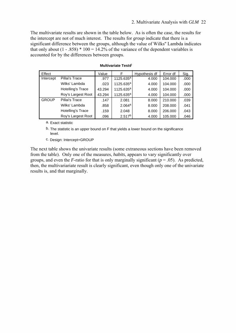
The multivariate results are shown in the table below. As is often the case, the results for the intercept are not of much interest. The results for group indicate that there is a significant difference between the groups, although the value of Wilks'' Lambda indicates that only about (1 - .858) * 100 = 14.2% of the variance of the dependent variables is accounted for by the differences between groups.
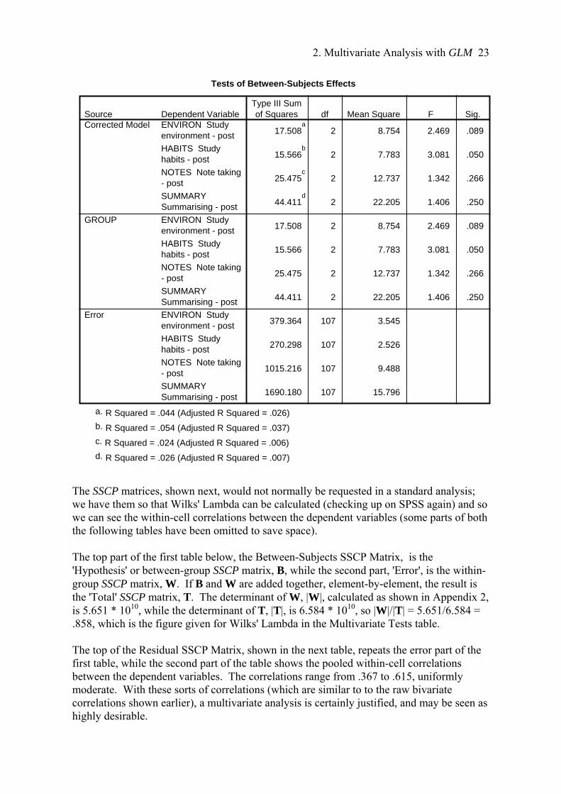
The next table shows the univariate results (some extraneous sections have been removed from the table). Only one of the measures, habits, appears to vary significantly over groups, and even the F-ratio for that is only marginally significant (p = .05). As predicted, then, the multivariariate result is clearly significant, even though only one of the univariate results is, and that marginally.
2. Multivariate Analysis with GLM 23
Tests of Between-Subjects Effects
17.508a
2 8.754 2.469 .089
15.566b
2 7.783 3.081 .050
25.475c
2 12.737 1.342 .266
44.411d
2 22.205 1.406 .250
17.508 2 8.754 2.469 .089
15.566 2 7.783 3.081 .050
25.475 2 12.737 1.342 .266
44.411 2 22.205 1.406 .250
379.364 107 3.545
270.298 107 2.526
1015.216 107 9.488
1690.180 107 15.796
Dependent VariableENVIRON Studyenvironment - post
HABITS Studyhabits - post
NOTES Note taking- post
SUMMARY Summarising - post
ENVIRON Studyenvironment - post
HABITS Studyhabits - post
NOTES Note taking- post
SUMMARY Summarising - post
ENVIRON Studyenvironment - post
HABITS Studyhabits - post
NOTES Note taking- post
SUMMARY Summarising - post
SourceCorrected Model
GROUP
Error
Type III Sumof Squares df Mean Square F Sig.
R Squared = .044 (Adjusted R Squared = .026)a.
R Squared = .054 (Adjusted R Squared = .037)b.
R Squared = .024 (Adjusted R Squared = .006)c.
R Squared = .026 (Adjusted R Squared = .007)d.
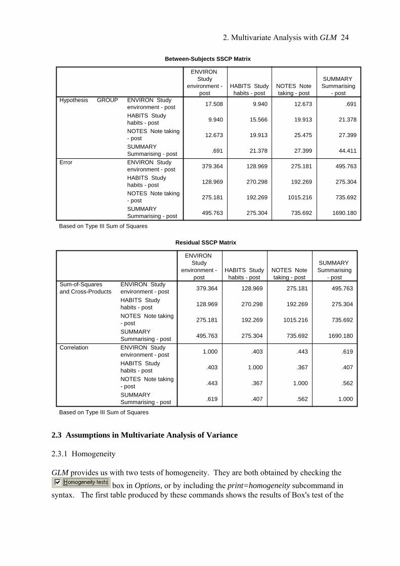
The SSCP matrices, shown next, would not normally be requested in a standard analysis; we have them so that Wilks' Lambda can be calculated (checking up on SPSS again) and so we can see the within-cell correlations between the dependent variables (some parts of both the following tables have been omitted to save space). The top part of the first table below, the Between-Subjects SSCP Matrix, is the 'Hypothesis' or between-group SSCP matrix, B, while the second part, 'Error', is the within-group SSCP matrix, W. If B and W are added together, element-by-element, the result is the 'Total' SSCP matrix, T. The determinant of W, |W|, calculated as shown in Appendix 2, is 5.651 * 1010, while the determinant of T, |T|, is 6.584 * 1010, so |W|/|T| = 5.651/6.584 = .858, which is the figure given for Wilks' Lambda in the Multivariate Tests table. The top of the Residual SSCP Matrix, shown in the next table, repeats the error part of the first table, while the second part of the table shows the pooled within-cell correlations between the dependent variables. The correlations range from .367 to .615, uniformly moderate. With these sorts of correlations (which are similar to to the raw bivariate correlations shown earlier), a multivariate analysis is certainly justified, and may be seen as highly desirable.
2. Multivariate Analysis with GLM 24
Between-Subjects SSCP Matrix
17.508 9.940 12.673 .691
9.940 15.566 19.913 21.378
12.673 19.913 25.475 27.399
.691 21.378 27.399 44.411
379.364 128.969 275.181 495.763
128.969 270.298 192.269 275.304
275.181 192.269 1015.216 735.692
495.763 275.304 735.692 1690.180
ENVIRON Studyenvironment - post
HABITS Studyhabits - post
NOTES Note taking- post
SUMMARY Summarising - post
ENVIRON Studyenvironment - post
HABITS Studyhabits - post
NOTES Note taking- post
SUMMARY Summarising - post
GROUPHypothesis
Error
ENVIRON Study
environment -post
HABITS Studyhabits - post
NOTES Notetaking - post
SUMMARY Summarising
- post
Based on Type III Sum of Squares
Residual SSCP Matrix
379.364 128.969 275.181 495.763
128.969 270.298 192.269 275.304
275.181 192.269 1015.216 735.692
495.763 275.304 735.692 1690.180
1.000 .403 .443 .619
.403 1.000 .367 .407
.443 .367 1.000 .562
.619 .407 .562 1.000
ENVIRON Studyenvironment - post
HABITS Studyhabits - post
NOTES Note taking- post
SUMMARY Summarising - post
ENVIRON Studyenvironment - post
HABITS Studyhabits - post
NOTES Note taking- post
SUMMARY Summarising - post
Sum-of-Squaresand Cross-Products
Correlation
ENVIRON Study
environment -post
HABITS Studyhabits - post
NOTES Notetaking - post
SUMMARY Summarising
- post
Based on Type III Sum of Squares
2.3 Assumptions in Multivariate Analysis of Variance 2.3.1 Homogeneity GLM provides us with two tests of homogeneity. They are both obtained by checking the
box in Options, or by including the print=homogeneity subcommand in syntax. The first table produced by these commands shows the results of Box's test of the
2. Multivariate Analysis with GLM 25
Box's Test of Equality of Covariance Matricesa
26.286
1.243
20
39644.836
.207
Box's M
F
df1
df2
Sig.
Tests the null hypothesis that the observed covariancematrices of the dependent variables are equal across groups.
Design: Intercept+GROUPa.
Levene's Test of Equality of Error Variancesa
.148 2 107 .920
.523 2 107 .592
.614 2 107 .539
2.000 2 107 .175
ENVIRON Studyenvironment - post
HABITS Studyhabits - post
NOTES Note taking- post
SUMMARY Summarising - post
F df1 df2 Sig.
Tests the null hypothesis that the error variance of thedependent variable is equal across groups.
Design: Intercept+GROUPa.
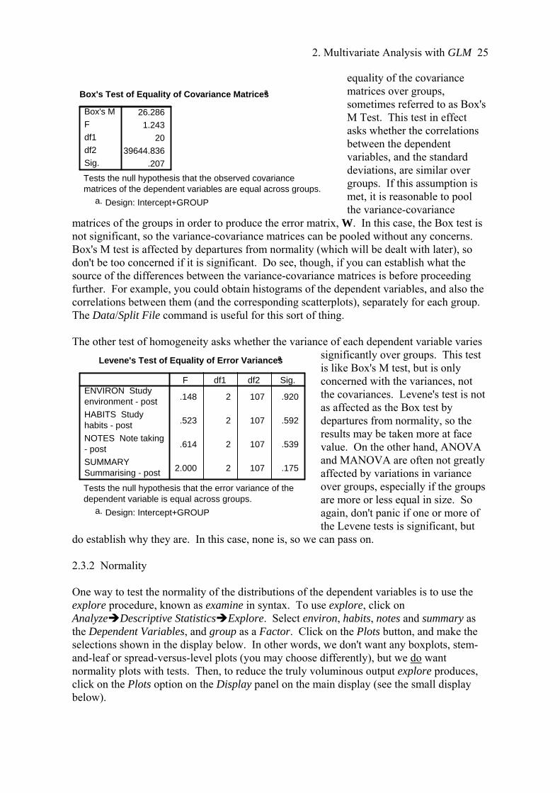
equality of the covariance matrices over groups, sometimes referred to as Box's M Test. This test in effect asks whether the correlations between the dependent variables, and the standard deviations, are similar over groups. If this assumption is met, it is reasonable to pool the variance-covariance
matrices of the groups in order to produce the error matrix, W. In this case, the Box test is not significant, so the variance-covariance matrices can be pooled without any concerns. Box's M test is affected by departures from normality (which will be dealt with later), so don't be too concerned if it is significant. Do see, though, if you can establish what the source of the differences between the variance-covariance matrices is before proceeding further. For example, you could obtain histograms of the dependent variables, and also the correlations between them (and the corresponding scatterplots), separately for each group. The Data/Split File command is useful for this sort of thing. The other test of homogeneity asks whether the variance of each dependent variable varies
significantly over groups. This test is like Box's M test, but is only concerned with the variances, not the covariances. Levene's test is not as affected as the Box test by departures from normality, so the results may be taken more at face value. On the other hand, ANOVA and MANOVA are often not greatly affected by variations in variance over groups, especially if the groups are more or less equal in size. So again, don't panic if one or more of the Levene tests is significant, but
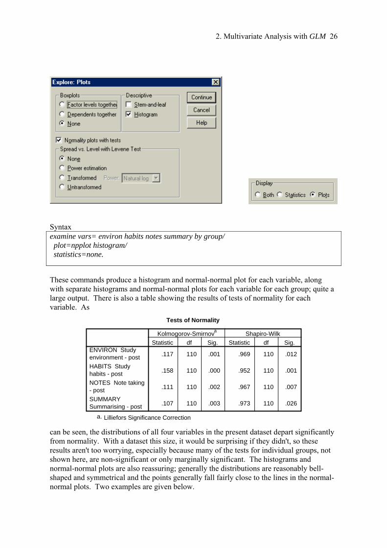
do establish why they are. In this case, none is, so we can pass on. 2.3.2 Normality One way to test the normality of the distributions of the dependent variables is to use the explore procedure, known as examine in syntax. To use explore, click on AnalyzeDescriptive StatisticsExplore. Select environ, habits, notes and summary as the Dependent Variables, and group as a Factor. Click on the Plots button, and make the selections shown in the display below. In other words, we don't want any boxplots, stem-and-leaf or spread-versus-level plots (you may choose differently), but we do want normality plots with tests. Then, to reduce the truly voluminous output explore produces, click on the Plots option on the Display panel on the main display (see the small display below).
2. Multivariate Analysis with GLM 26
Syntax examine vars= environ habits notes summary by group/ plot=npplot histogram/ statistics=none.
These commands produce a histogram and normal-normal plot for each variable, along with separate histograms and normal-normal plots for each variable for each group; quite a large output. There is also a table showing the results of tests of normality for each variable. As
Tests of Normality
.117 110 .001 .969 110 .012
.158 110 .000 .952 110 .001
.111 110 .002 .967 110 .007
.107 110 .003 .973 110 .026
ENVIRON Studyenvironment - post
HABITS Studyhabits - post
NOTES Note taking- post
SUMMARY Summarising - post
Statistic df Sig. Statistic df Sig.
Kolmogorov-Smirnova
Shapiro-Wilk
Lilliefors Significance Correctiona.
can be seen, the distributions of all four variables in the present dataset depart significantly from normality. With a dataset this size, it would be surprising if they didn't, so these results aren't too worrying, especially because many of the tests for individual groups, not shown here, are non-significant or only marginally significant. The histograms and normal-normal plots are also reassuring; generally the distributions are reasonably bell-shaped and symmetrical and the points generally fall fairly close to the lines in the normal-normal plots. Two examples are given below.
2. Multivariate Analysis with GLM 27
Study environment - post
14.012.010.08.06.04.0
Histogram
Fre
quen
cy
50
40
30
20
10
0
Std. Dev = 1.91
Mean = 8.3
N = 110.00
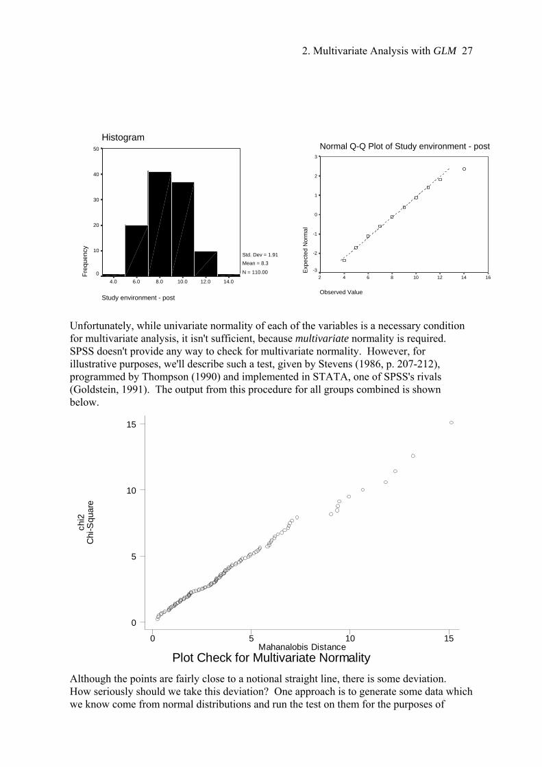
Unfortunately, while univariate normality of each of the variables is a necessary condition for multivariate analysis, it isn't sufficient, because multivariate normality is required. SPSS doesn't provide any way to check for multivariate normality. However, for illustrative purposes, we'll describe such a test, given by Stevens (1986, p. 207-212), programmed by Thompson (1990) and implemented in STATA, one of SPSS's rivals (Goldstein, 1991). The output from this procedure for all groups combined is shown below.
chi2
Chi
-Squ
are
Plot Check for Multivariate NormalityMahanalobis Distance
0 5 10 15
0
5
10
15
Although the points are fairly close to a notional straight line, there is some deviation. How seriously should we take this deviation? One approach is to generate some data which we know come from normal distributions and run the test on them for the purposes of
Normal Q-Q Plot of Study environment - post
Observed Value
161412108642
Exp
ecte
d N
orm
al
3
2
1
0
-1
-2
-3
2. Multivariate Analysis with GLM 28
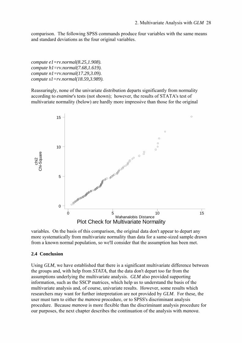
comparison. The following SPSS commands produce four variables with the same means and standard deviations as the four original variables. compute e1=rv.normal(8.25,1.908). compute h1=rv.normal(7.68,1.619). compute n1=rv.normal(17.29,3.09). compute s1=rv.normal(18.59,3.989). Reassuringly, none of the univariate distribution departs significantly from normality according to examine's tests (not shown); however, the results of STATA's test of multivariate normality (below) are hardly more impressive than those for the original
chi2
Chi
-Squ
are
Plot Check for Multivariate NormalityMahanalobis Distance
0 5 10 15
0
5
10
15
variables. On the basis of this comparison, the original data don't appear to depart any more systematically from multivariate normality than data for a same-sized sample drawn from a known normal population, so we'll consider that the assumption has been met. 2.4 Conclusion Using GLM, we have established that there is a significant multivariate difference between the groups and, with help from STATA, that the data don't depart too far from the assumptions underlying the multivariate analysis. GLM also provided supporting information, such as the SSCP matrices, which help us to understand the basis of the multivariate analysis and, of course, univariate results. However, some results which researchers may want for further interpretation are not provided by GLM. For these, the user must turn to either the manova procedure, or to SPSS's discriminant analysis procedure. Because manova is more flexible than the discriminant analysis procedure for our purposes, the next chapter describes the continuation of the analysis with manova.
3. Multivariate Analysis with manova 29
3. Multivariate Analysis with the manova procedure Since the advent of GLM, the manova procedure is usable only with syntax; however, manova provides information for the interpretation of the multivariate results which GLM doesn't. The syntax below could be used to carry out a multivariate analysis of variance on the data used in Section 2 which would provide everything that GLM did (or equivalents), plus some extras which are very useful in interpreting the multivariate results. manova environ habits notes summary by group(0,2)/ contrast(group)=simple(1)/ print=signif(multiv univ hypoth dimenr eigen) homog(all) cellinfo(corr sscp) error(corr sscp)/ discrim=all/ design. For our purposes, we'll run the following reduced syntax, which doesn't reproduce everything that GLM did, but just things which GLM didn’t produce (a noprint subcommand in GLM would be handy). manova environ habits notes summary by group(0,2)/ contrast(group)=simple(1)/ print=signif(dimenr eigen) cellinfo(corr sscp) error(corr)/ noprint=signif(multiv univ hypoth)/ discrim=all/ design. The output is shown below. Comments will be inserted into the output in boxes, so they are clearly distinguishable from the manova results. Generally the boxes precede the parts of the output they refer to. Manova The default error term in MANOVA has been changed from WITHIN CELLS to WITHIN+RESIDUAL. Note that these are the same for all full factorial designs. * * * * * * A n a l y s i s o f V a r i a n c e * * * * * * 110 cases accepted. 0 cases rejected because of out-of-range factor values. 0 cases rejected because of missing data. 3 non-empty cells. 1 design will be processed. - - - - - - - - - - - - - - - - - - - - - - - - - - - - - - - - - - - -
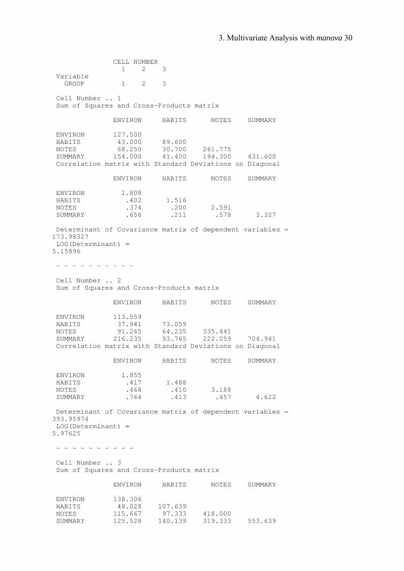
As a result of the cellinfo(corr sscp) commands in the print subcommand, manova prints out the correlations between the dependent variables, the SSCP matrices for each group. In the event of a significant result for Box's M, this output makes it possible to compare standard deviations, correlations and SSs over groups to find the source of the differences between the matrices.
3. Multivariate Analysis with manova 30
CELL NUMBER 1 2 3 Variable GROUP 1 2 3 Cell Number .. 1 Sum of Squares and Cross-Products matrix ENVIRON HABITS NOTES SUMMARY ENVIRON 127.500 HABITS 43.000 89.600 NOTES 68.250 30.700 261.775 SUMMARY 154.000 41.400 194.300 431.600 Correlation matrix with Standard Deviations on Diagonal ENVIRON HABITS NOTES SUMMARY ENVIRON 1.808 HABITS .402 1.516 NOTES .374 .200 2.591 SUMMARY .656 .211 .578 3.327 Determinant of Covariance matrix of dependent variables = 173.98327 LOG(Determinant) = 5.15896 - - - - - - - - - - Cell Number .. 2 Sum of Squares and Cross-Products matrix ENVIRON HABITS NOTES SUMMARY ENVIRON 113.559 HABITS 37.941 73.059 NOTES 91.265 64.235 335.441 SUMMARY 216.235 93.765 222.059 704.941 Correlation matrix with Standard Deviations on Diagonal ENVIRON HABITS NOTES SUMMARY ENVIRON 1.855 HABITS .417 1.488 NOTES .468 .410 3.188 SUMMARY .764 .413 .457 4.622 Determinant of Covariance matrix of dependent variables = 393.95974 LOG(Determinant) = 5.97625 - - - - - - - - - - Cell Number .. 3 Sum of Squares and Cross-Products matrix ENVIRON HABITS NOTES SUMMARY ENVIRON 138.306 HABITS 48.028 107.639 NOTES 115.667 97.333 418.000 SUMMARY 125.528 140.139 319.333 553.639

3. Multivariate Analysis with manova 31
Correlation matrix with Standard Deviations on Diagonal ENVIRON HABITS NOTES SUMMARY ENVIRON 1.988 HABITS .394 1.754 NOTES .481 .459 3.456 SUMMARY .454 .574 .664 3.977 Determinant of Covariance matrix of dependent variables = 608.70972 LOG(Determinant) = 6.41134 - - - - - - - - - - Determinant of pooled Covariance matrix of dependent vars. = 431.09880 LOG(Determinant) = 6.06634 - - - - - - - - - - - - - - - - - - - - - - - - - - - - - - - - - - - - WITHIN CELLS Correlations with Std. Devs. on Diagonal ENVIRON HABITS NOTES SUMMARY ENVIRON 1.883 HABITS .403 1.589 NOTES .443 .367 3.080 SUMMARY .619 .407 .562 3.974 - - - - - - - - - - - - - - - - - - - - - - - - - - - - - - - - - - - - Statistics for WITHIN CELLS correlations Log(Determinant) = -1.13582 Bartlett test of sphericity = 119.07135 with 6 D. F. Significance = .000 F(max) criterion = 6.25303 with (4,107) D. F. - - - - - - - - - - - - - - - - - - - - - - - - - - - - - - - - - - - -
The following table shows the two eigenvalues of the BW-1 matrix. They can be used to calculate the multivariate statistics shown in Section 1.7 as follows: Wilks' Lambda: 1/(1 + λ1) * 1/(1 + λ2) = 1/(1 + .096) * 1/(1 + .063) = .858 Pillais Trace: λ1/(1 + λ1) + λ2/(1 + λ2) = .096/(1 + .096) + .063/(1 + .063) = .147 Hotelling-Lawley = λ1 + λ2 = .096 + .063 = .159 Roy's Largest Root: λ1 = .096
3. Multivariate Analysis with manova 32
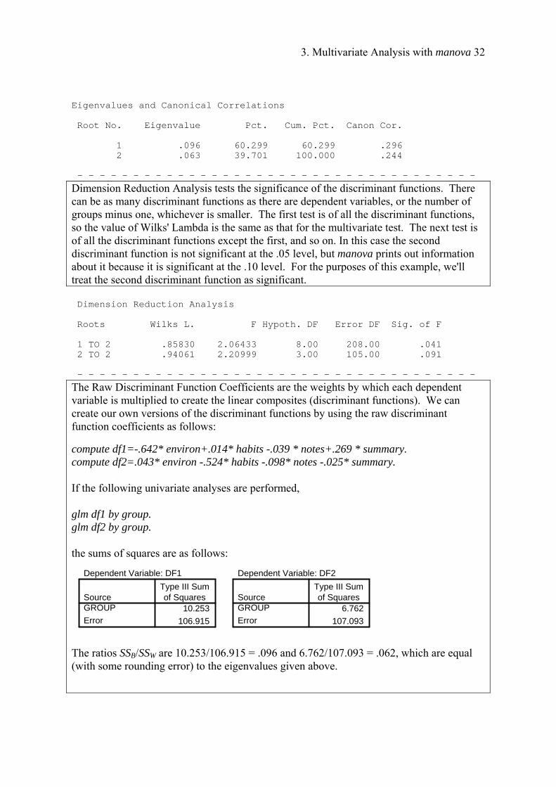
Eigenvalues and Canonical Correlations Root No. Eigenvalue Pct. Cum. Pct. Canon Cor. 1 .096 60.299 60.299 .296 2 .063 39.701 100.000 .244 - - - - - - - - - - - - - - - - - - - - - - - - - - - - - - - - - - - -
Dimension Reduction Analysis tests the significance of the discriminant functions. There can be as many discriminant functions as there are dependent variables, or the number of groups minus one, whichever is smaller. The first test is of all the discriminant functions, so the value of Wilks' Lambda is the same as that for the multivariate test. The next test is of all the discriminant functions except the first, and so on. In this case the second discriminant function is not significant at the .05 level, but manova prints out information about it because it is significant at the .10 level. For the purposes of this example, we'll treat the second discriminant function as significant. Dimension Reduction Analysis Roots Wilks L. F Hypoth. DF Error DF Sig. of F 1 TO 2 .85830 2.06433 8.00 208.00 .041 2 TO 2 .94061 2.20999 3.00 105.00 .091 - - - - - - - - - - - - - - - - - - - - - - - - - - - - - - - - - - - -
The Raw Discriminant Function Coefficients are the weights by which each dependent variable is multiplied to create the linear composites (discriminant functions). We can create our own versions of the discriminant functions by using the raw discriminant function coefficients as follows:
compute df1=-.642* environ+.014* habits -.039 * notes+.269 * summary. compute df2=.043* environ -.524* habits -.098* notes -.025* summary. If the following univariate analyses are performed, glm df1 by group. glm df2 by group. the sums of squares are as follows:
Dependent Variable: DF1
10.253
106.915
SourceGROUP
Error
Type III Sumof Squares
Dependent Variable: DF2
6.762
107.093
SourceGROUP
Error
Type III Sumof Squares
The ratios SSB/SSW are 10.253/106.915 = .096 and 6.762/107.093 = .062, which are equal (with some rounding error) to the eigenvalues given above.
3. Multivariate Analysis with manova 33
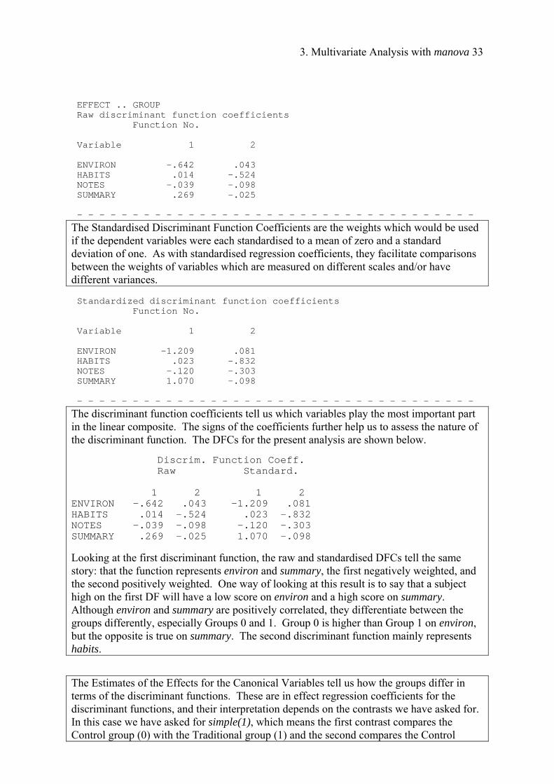
EFFECT .. GROUP Raw discriminant function coefficients Function No. Variable 1 2 ENVIRON -.642 .043 HABITS .014 -.524 NOTES -.039 -.098 SUMMARY .269 -.025 - - - - - - - - - - - - - - - - - - - - - - - - - - - - - - - - - - - -
The Standardised Discriminant Function Coefficients are the weights which would be used if the dependent variables were each standardised to a mean of zero and a standard deviation of one. As with standardised regression coefficients, they facilitate comparisons between the weights of variables which are measured on different scales and/or have different variances. Standardized discriminant function coefficients Function No. Variable 1 2 ENVIRON -1.209 .081 HABITS .023 -.832 NOTES -.120 -.303 SUMMARY 1.070 -.098 - - - - - - - - - - - - - - - - - - - - - - - - - - - - - - - - - - - -
The discriminant function coefficients tell us which variables play the most important part in the linear composite. The signs of the coefficients further help us to assess the nature of the discriminant function. The DFCs for the present analysis are shown below. Discrim. Function Coeff. Raw Standard. 1 2 1 2 ENVIRON -.642 .043 -1.209 .081 HABITS .014 -.524 .023 -.832 NOTES -.039 -.098 -.120 -.303 SUMMARY .269 -.025 1.070 -.098
Looking at the first discriminant function, the raw and standardised DFCs tell the same story: that the function represents environ and summary, the first negatively weighted, and the second positively weighted. One way of looking at this result is to say that a subject high on the first DF will have a low score on environ and a high score on summary. Although environ and summary are positively correlated, they differentiate between the groups differently, especially Groups 0 and 1. Group 0 is higher than Group 1 on environ, but the opposite is true on summary. The second discriminant function mainly represents habits.
The Estimates of the Effects for the Canonical Variables tell us how the groups differ in terms of the discriminant functions. These are in effect regression coefficients for the discriminant functions, and their interpretation depends on the contrasts we have asked for. In this case we have asked for simple(1), which means the first contrast compares the Control group (0) with the Traditional group (1) and the second compares the Control
3. Multivariate Analysis with manova 34
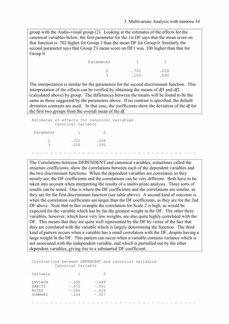
group with the Audio-visual group (2). Looking at the estimates of the effects for the canonical variables below, the first parameter for the 1st DF says that the mean score on that function is .702 higher for Group 1 than the mean DF for Group 0. Similarly the second parameter says that Group 2's mean score on DF1 was .100 higher than that for Group 0. Parameter 1 2 2 .702 .208 3 .100 .592
The interpretation is similar for the parameters for the second discriminant function. This interpretation of the effects can be verified by obtaining the means of df1 and df2 (calculated above) by group. The differences between the means will be found to be the same as those suggested by the parameters above. If no contrast is specified, the default deviation contrasts are used. In that case, the coefficients show the deviation of the df for the first two groups from the overall mean of the df. Estimates of effects for canonical variables Canonical Variable Parameter 1 2 2 .702 .208 3 .100 .592 - - - - - - - - - - - - - - - - - - - - - - - - - - - - - - - - - - - -
The Correlations between DEPENDENT and canonical variables, sometimes called the structure coefficients, show the correlations between each of the dependent variables and the two discriminant functions. When the dependent variables are correlated, as they mostly are, the DF coefficients and the correlations can be very different. Both have to be taken into account when interpreting the results of a multivariate analysis. Three sorts of results can be noted. One is where the DF coefficients and the correlations are similar, as they are for the first discriminant function (see table above). A second kind of outcome is when the correlation coefficients are larger than the DF coefficients, as they are for the 2nd DF above. Note that in this example the correlation for Scale 2 is high, as would be expected for the variable which has by far the greatest weight in the DF. The other three variables, however, which have very low weights, are also quite highly correlated with the DF. This means that they are quite well represented by the DF by virtue of the fact that they are correlated with the variable which is largely determining the function. The third kind of pattern occurs when a variable has a small correlation with the DF, despite having a large weight in the DF. This pattern can occur when a variable contains variance which is not associated with the independent variable, and which is partialled out by the other dependent variables, giving rise to a substantial DF coefficient. Correlations between DEPENDENT and canonical variables Canonical Variable Variable 1 2 ENVIRON -.590 -.449 HABITS -.072 -.951 NOTES -.046 -.628 SUMMARY .264 -.557 - - - - - - - - - - - - - - - - - - - - - - - - - - - - - - - - - - - -
3. Multivariate Analysis with manova 35
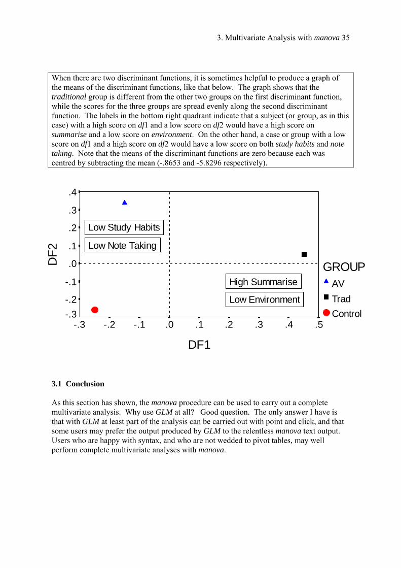
When there are two discriminant functions, it is sometimes helpful to produce a graph of the means of the discriminant functions, like that below. The graph shows that the traditional group is different from the other two groups on the first discriminant function, while the scores for the three groups are spread evenly along the second discriminant function. The labels in the bottom right quadrant indicate that a subject (or group, as in this case) with a high score on df1 and a low score on df2 would have a high score on summarise and a low score on environment. On the other hand, a case or group with a low score on df1 and a high score on df2 would have a low score on both study habits and note taking. Note that the means of the discriminant functions are zero because each was centred by subtracting the mean (-.8653 and -5.8296 respectively).
3.1 Conclusion As this section has shown, the manova procedure can be used to carry out a complete multivariate analysis. Why use GLM at all? Good question. The only answer I have is that with GLM at least part of the analysis can be carried out with point and click, and that some users may prefer the output produced by GLM to the relentless manova text output. Users who are happy with syntax, and who are not wedded to pivot tables, may well perform complete multivariate analyses with manova.
GROUPAV
Trad
Control
DF1
.5.4.3.2.1.0-.1-.2-.3
DF
2
.4
.3
.2
.1
.0
-.1
-.2
-.3
Low Environment
High Summarise
Low Study Habits
Low Note Taking
3. Multivariate Analysis with manova 36
4. Following up Multivariate Analysis 37
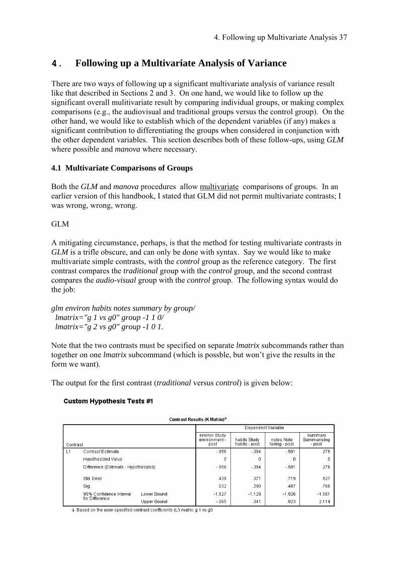
4. Following up a Multivariate Analysis of Variance There are two ways of following up a significant multivariate analysis of variance result like that described in Sections 2 and 3. On one hand, we would like to follow up the significant overall mulitivariate result by comparing individual groups, or making complex comparisons (e.g., the audiovisual and traditional groups versus the control group). On the other hand, we would like to establish which of the dependent variables (if any) makes a significant contribution to differentiating the groups when considered in conjunction with the other dependent variables. This section describes both of these follow-ups, using GLM where possible and manova where necessary. 4.1 Multivariate Comparisons of Groups Both the GLM and manova procedures allow multivariate comparisons of groups. In an earlier version of this handbook, I stated that GLM did not permit multivariate contrasts; I was wrong, wrong, wrong. GLM A mitigating circumstance, perhaps, is that the method for testing multivariate contrasts in GLM is a trifle obscure, and can only be done with syntax. Say we would like to make multivariate simple contrasts, with the control group as the reference category. The first contrast compares the traditional group with the control group, and the second contrast compares the audio-visual group with the control group. The following syntax would do the job: glm environ habits notes summary by group/ lmatrix="g 1 vs g0" group -1 1 0/ lmatrix="g 2 vs g0" group -1 0 1. Note that the two contrasts must be specified on separate lmatrix subcommands rather than together on one lmatrix subcommand (which is possble, but won’t give the results in the form we want). The output for the first contrast (traditional versus control) is given below:
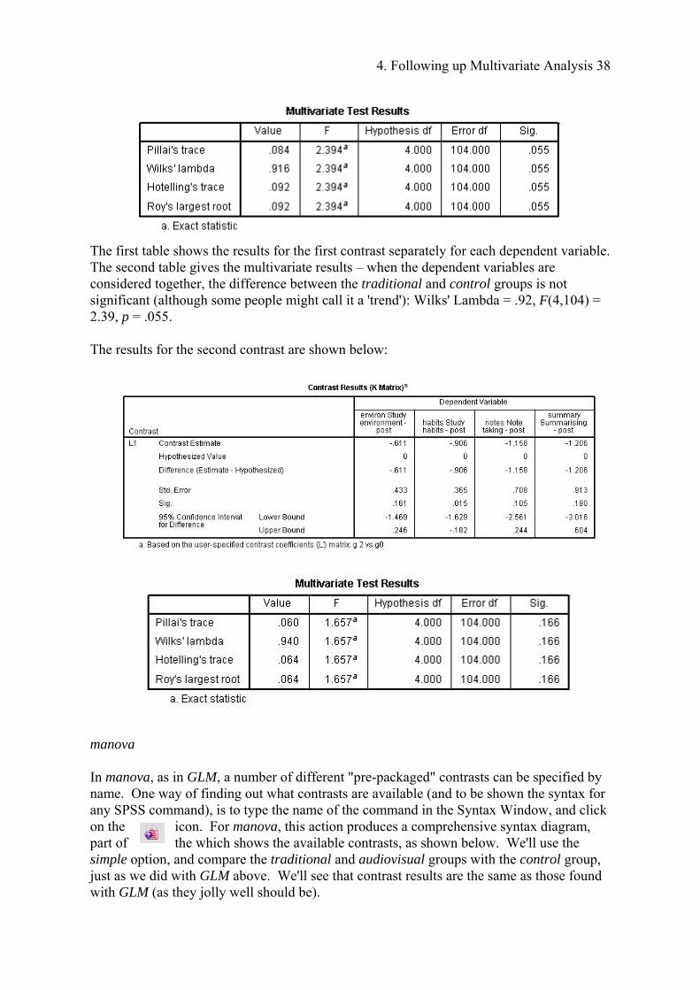
4. Following up Multivariate Analysis 38
The first table shows the results for the first contrast separately for each dependent variable. The second table gives the multivariate results – when the dependent variables are considered together, the difference between the traditional and control groups is not significant (although some people might call it a 'trend'): Wilks' Lambda = .92, F(4,104) = 2.39, p = .055. The results for the second contrast are shown below: manova In manova, as in GLM, a number of different "pre-packaged" contrasts can be specified by name. One way of finding out what contrasts are available (and to be shown the syntax for any SPSS command), is to type the name of the command in the Syntax Window, and click on the icon. For manova, this action produces a comprehensive syntax diagram, part of the which shows the available contrasts, as shown below. We'll use the simple option, and compare the traditional and audiovisual groups with the control group, just as we did with GLM above. We'll see that contrast results are the same as those found with GLM (as they jolly well should be).

4. Following up Multivariate Analysis 39
The syntax shown below makes use of a manova feature which allows individual contrasts to be specified in the design sub-command. Because the contrast(group)=simple(1) sub-command specifies the comparison of each group with the lowest-numbered group (i.e., the control group), the group(1) keyword in the design sub-command refers to the comparison of the traditional group with the control group, and the group(2) keyword refers to the comparison of the audiovisual group with the control group. manova environ habits notes summary by group(0,2)/ contrast(group)=simple(1)/ print=signif(multiv univ)/ discrim=all/ design=group(1) group(2). The full output is shown below. Comments are given in boxes. * * * * * * A n a l y s i s o f V a r i a n c e * * * * * * 110 cases accepted. 0 cases rejected because of out-of-range factor values. 0 cases rejected because of missing data. 3 non-empty cells. 1 design will be processed. - - - - - - - - - - - - - - - - - - - - - - - - - - - - - - - - - - - - -

4. Following up Multivariate Analysis 40
* * * * * * A n a l y s i s o f V a r i a n c e -- design 1 * * * * * *
The first multivariate analysis tests the difference between the audiovisual and control groups (the manova output starts with the contrast or effect named last on the design sub-command). The difference is clearly non-significant, even before any allowance is made for the number of contrasts actually performed (the a priori approach) or which could have been performed (post-hoc). Although the univariate results are not now of interest, it's worth noting that if the groups differ on anything, they do so on study habits. The standardised discriminant coefficients show that the measure of study habits is the best discriminator of the audivisual and control groups even when adjusted for the other variables. The negative sign of the coefficient for habits means that a group with a high discriminant function score will have a relatively low score on habits. The estimate of the effect for the single discriminant function, .600, means that the audiovisal group's score on the DF was 0.6 higher than that for the control group (the score for the reference group is subtracted from that for the group which is being compared to it), meaning that the control group had a higher score on habits than the audiovisual group. The uniformly substantial correlations between the dependent variables and the discriminant function suggest that the DF "represents" all of the dependent variables, despite habits having by far the highest standardised discriminant function coefficient. The negative signs on the coefficients show that each variable discriminates between the audiovisual and control groups in the same way; i.e., the score on each is lower for the audiovisual group than for the control group. This raises an important point: when carrying out comparisons between two groups, the multivariate analysis arrives at coefficients for the dependent variables which maximise the difference between just those two groups (or combinations of groups), so that the pattern of the discriminant function coefficients may be very different from that for the overall test of the differences between the groups and also for that for the test of the difference between any other pair of groups. EFFECT .. GROUP(2) Multivariate Tests of Significance (S = 1, M = 1 , N = 51 ) Test Name Value Exact F Hypoth. DF Error DF Sig. of F Pillais .05992 1.65735 4.00 104.00 .166 Hotellings .06374 1.65735 4.00 104.00 .166 Wilks .94008 1.65735 4.00 104.00 .166 Roys .05992 Note.. F statistics are exact. - - - - - - - - - - - - - - - - - - - - - - - - - - - - - - - - - - - - - EFFECT .. GROUP(2) (Cont.) Univariate F-tests with (1,107) D. F. Variable Hypoth. SS Error SS Hypoth. MS Error MS F Sig. of F ENVIRON 7.07602 379.36438 7.07602 3.54546 1.99580 .161 HABITS 15.53743 270.29771 15.53743 2.52615 6.15064 .015 NOTES 25.42237 1015.21618 25.42237 9.48800 2.67942 .105 SUMMARY 27.53743 1690.18007 27.53743 15.79608 1.74331 .190 - - - - - - - - - - - - - - - - - - - - - - - - - - - - - - - - - - - - - EFFECT .. GROUP(2) (Cont.) Raw discriminant function coefficients Function No. Variable 1 ENVIRON -.064 HABITS -.514 NOTES -.104 SUMMARY .020
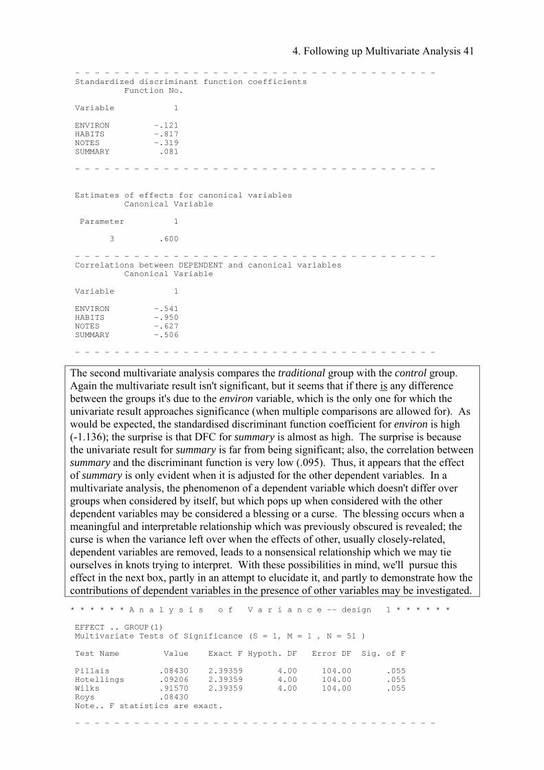
4. Following up Multivariate Analysis 41
- - - - - - - - - - - - - - - - - - - - - - - - - - - - - - - - - - - - - Standardized discriminant function coefficients Function No. Variable 1 ENVIRON -.121 HABITS -.817 NOTES -.319 SUMMARY .081 - - - - - - - - - - - - - - - - - - - - - - - - - - - - - - - - - - - - - Estimates of effects for canonical variables Canonical Variable Parameter 1 3 .600 - - - - - - - - - - - - - - - - - - - - - - - - - - - - - - - - - - - - - Correlations between DEPENDENT and canonical variables Canonical Variable Variable 1 ENVIRON -.541 HABITS -.950 NOTES -.627 SUMMARY -.506 - - - - - - - - - - - - - - - - - - - - - - - - - - - - - - - - - - - - -
The second multivariate analysis compares the traditional group with the control group. Again the multivariate result isn't significant, but it seems that if there is any difference between the groups it's due to the environ variable, which is the only one for which the univariate result approaches significance (when multiple comparisons are allowed for). As would be expected, the standardised discriminant function coefficient for environ is high (-1.136); the surprise is that DFC for summary is almost as high. The surprise is because the univariate result for summary is far from being significant; also, the correlation between summary and the discriminant function is very low (.095). Thus, it appears that the effect of summary is only evident when it is adjusted for the other dependent variables. In a multivariate analysis, the phenomenon of a dependent variable which doesn't differ over groups when considered by itself, but which pops up when considered with the other dependent variables may be considered a blessing or a curse. The blessing occurs when a meaningful and interpretable relationship which was previously obscured is revealed; the curse is when the variance left over when the effects of other, usually closely-related, dependent variables are removed, leads to a nonsensical relationship which we may tie ourselves in knots trying to interpret. With these possibilities in mind, we'll pursue this effect in the next box, partly in an attempt to elucidate it, and partly to demonstrate how the contributions of dependent variables in the presence of other variables may be investigated. * * * * * * A n a l y s i s o f V a r i a n c e -- design 1 * * * * * * EFFECT .. GROUP(1) Multivariate Tests of Significance (S = 1, M = 1 , N = 51 ) Test Name Value Exact F Hypoth. DF Error DF Sig. of F Pillais .08430 2.39359 4.00 104.00 .055 Hotellings .09206 2.39359 4.00 104.00 .055 Wilks .91570 2.39359 4.00 104.00 .055 Roys .08430 Note.. F statistics are exact. - - - - - - - - - - - - - - - - - - - - - - - - - - - - - - - - - - - - -
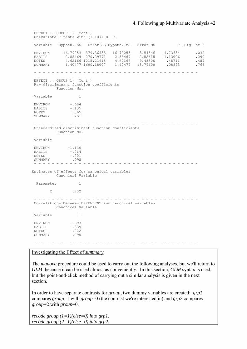
4. Following up Multivariate Analysis 42
EFFECT .. GROUP(1) (Cont.) Univariate F-tests with (1,107) D. F. Variable Hypoth. SS Error SS Hypoth. MS Error MS F Sig. of F ENVIRON 16.79253 379.36438 16.79253 3.54546 4.73634 .032 HABITS 2.85469 270.29771 2.85469 2.52615 1.13006 .290 NOTES 4.62166 1015.21618 4.62166 9.48800 .48711 .487 SUMMARY 1.40477 1690.18007 1.40477 15.79608 .08893 .766 - - - - - - - - - - - - - - - - - - - - - - - - - - - - - - - - - - - - - EFFECT .. GROUP(1) (Cont.) Raw discriminant function coefficients Function No. Variable 1 ENVIRON -.604 HABITS -.135 NOTES -.065 SUMMARY .251 - - - - - - - - - - - - - - - - - - - - - - - - - - - - - - - - - - - - - Standardized discriminant function coefficients Function No. Variable 1 ENVIRON -1.136 HABITS -.214 NOTES -.201 SUMMARY .998 - - - - - - - - - - - - - - - - - - - - - - - - - - - - - - - - - - - - - Estimates of effects for canonical variables Canonical Variable Parameter 1 2 .732 - - - - - - - - - - - - - - - - - - - - - - - - - - - - - - - - - - - - - Correlations between DEPENDENT and canonical variables Canonical Variable Variable 1 ENVIRON -.693 HABITS -.339 NOTES -.222 SUMMARY .095 - - - - - - - - - - - - - - - - - - - - - - - - - - - - - - - - - - - - -
Investigating the Effect of summary The manova procedure could be used to carry out the following analyses, but we'll return to GLM, because it can be used almost as conveniently. In this section, GLM syntax is used, but the point-and-click method of carrying out a similar analysis is given in the next section. In order to have separate contrasts for group, two dummy variables are created: grp1 compares group=1 with group=0 (the contrast we're interested in) and grp2 compares group=2 with group=0. recode group (1=1)(else=0) into grp1. recode group (2=1)(else=0) into grp2.

4. Following up Multivariate Analysis 43
The first analysis simply reproduces the univariate result as a reassurance that the coding is working appropriately: glm summary with grp1 grp2/ print=parameters.
Tests of Between-Subjects Effects
Dependent Variable: SUMMARY Summarising - post
44.411a 2 22.205 1.406 .250
1.405 1 1.405 .089 .766
27.537 1 27.537 1.743 .190
1690.180 107 15.796
1734.591 109
SourceCorrected Model
GRP1
GRP2
Error
Corrected Total
Type III Sumof Squares df Mean Square F Sig.
R Squared = .026 (Adjusted R Squared = .007)a.
Parameter Estimates
Dependent Variable: SUMMARY Summarising - post
18.900 .628 30.076 .000 17.654 20.146
.276 .927 .298 .766 -1.561 2.114
-1.206 .913 -1.320 .190 -3.016 .604
ParameterIntercept
GRP1
GRP2
B Std. Error t Sig. Lower Bound Upper Bound
95% Confidence Interval
The ANOVA table (with a bit of irrelevant material removed), confirms that the dummy coding is appropriate: the p-values for grp1 and grp2 are identical to those shown in the univariate output above. The Parameter Estimates table shows that the difference between the mean of summary for groups 1 and 0, unadjusted for any other variables, is .276. In the next step in the analysis, summary continues as the dependent variable, but the other dependent variables in the multivariate analysis are entered as covariates. This analysis assesses the difference between groups 1 and 0 in terms of summary when adjusted for environ, habits and notes. In other words, the analysis seeks to emulate the results of the multivariate analysis in a way which allows us to assess, in a different way, the unique contribution of summary to differentiating the groups in the presence of the other variables. glm summary with environ habits notes grp1 grp2/ print=parameters.
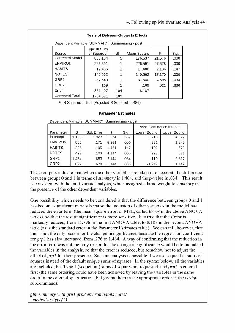
4. Following up Multivariate Analysis 44
Tests of Between-Subjects Effects
Dependent Variable: SUMMARY Summarising - post
883.184a 5 176.637 21.576 .000
226.591 1 226.591 27.678 .000
17.486 1 17.486 2.136 .147
140.562 1 140.562 17.170 .000
37.640 1 37.640 4.598 .034
.169 1 .169 .021 .886
851.407 104 8.187
1734.591 109
SourceCorrected Model
ENVIRON
HABITS
NOTES
GRP1
GRP2
Error
Corrected Total
Type III Sumof Squares df Mean Square F Sig.
R Squared = .509 (Adjusted R Squared = .486)a.
Parameter Estimates
Dependent Variable: SUMMARY Summarising - post
1.106 1.927 .574 .567 -2.715 4.927
.900 .171 5.261 .000 .561 1.240
.286 .195 1.461 .147 -.102 .673
.427 .103 4.144 .000 .222 .631
1.464 .683 2.144 .034 .110 2.817
.097 .678 .144 .886 -1.247 1.442
ParameterIntercept
ENVIRON
HABITS
NOTES
GRP1
GRP2
B Std. Error t Sig. Lower Bound Upper Bound
95% Confidence Interval
These outputs indicate that, when the other variables are taken into account, the difference between groups 0 and 1 in terms of summary is 1.464, and the p-value is .034. This result is consistent with the multivariate analysis, which assigned a large weight to summary in the presence of the other dependent variables. One possibility which needs to be considered is that the difference between groups 0 and 1 has become significant merely because the inclusion of other variables in the model has reduced the error term (the mean square error, or MSE, called Error in the above ANOVA tables), so that the test of significance is more sensitive. It is true that the Error is markedly reduced, from 15.796 in the first ANOVA table, to 8.187 in the second ANOVA table (as is the standard error in the Parameter Estimates table). We can tell, however, that this is not the only reason for the change in significance, because the regression coefficient for grp1 has also increased, from .276 to 1.464. A way of confirming that the reduction in the error term was not the only reason for the change in significance would be to include all the variables in the analysis, so that the error is reduced, but somehow not to adjust the effect of grp1 for their presence. Such an analysis is possible if we use sequential sums of squares instead of the default unique sums of squares. In the syntax below, all the variables are included, but Type 1 (sequential) sums of squares are requested, and grp1 is entered first (the same ordering could have been achieved by leaving the variables in the same order in the original specification, but giving them in the appropriate order in the design subcommand): glm summary with grp1 grp2 environ habits notes/ method=sstype(1).
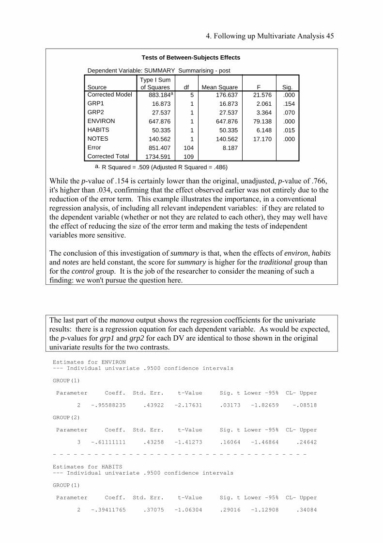
4. Following up Multivariate Analysis 45
Tests of Between-Subjects Effects
Dependent Variable: SUMMARY Summarising - post
883.184a 5 176.637 21.576 .000
16.873 1 16.873 2.061 .154
27.537 1 27.537 3.364 .070
647.876 1 647.876 79.138 .000
50.335 1 50.335 6.148 .015
140.562 1 140.562 17.170 .000
851.407 104 8.187
1734.591 109
SourceCorrected Model
GRP1
GRP2
ENVIRON
HABITS
NOTES
Error
Corrected Total
Type I Sumof Squares df Mean Square F Sig.
R Squared = .509 (Adjusted R Squared = .486)a.
While the p-value of .154 is certainly lower than the original, unadjusted, p-value of .766, it's higher than .034, confirming that the effect observed earlier was not entirely due to the reduction of the error term. This example illustrates the importance, in a conventional regression analysis, of including all relevant independent variables: if they are related to the dependent variable (whether or not they are related to each other), they may well have the effect of reducing the size of the error term and making the tests of independent variables more sensitive. The conclusion of this investigation of summary is that, when the effects of environ, habits and notes are held constant, the score for summary is higher for the traditional group than for the control group. It is the job of the researcher to consider the meaning of such a finding: we won't pursue the question here. The last part of the manova output shows the regression coefficients for the univariate results: there is a regression equation for each dependent variable. As would be expected, the p-values for grp1 and grp2 for each DV are identical to those shown in the original univariate results for the two contrasts. Estimates for ENVIRON --- Individual univariate .9500 confidence intervals GROUP(1) Parameter Coeff. Std. Err. t-Value Sig. t Lower -95% CL- Upper 2 -.95588235 .43922 -2.17631 .03173 -1.82659 -.08518 GROUP(2) Parameter Coeff. Std. Err. t-Value Sig. t Lower -95% CL- Upper 3 -.61111111 .43258 -1.41273 .16064 -1.46864 .24642 - - - - - - - - - - - - - - - - - - - - - - - - - - - - - - - - - - - - - Estimates for HABITS --- Individual univariate .9500 confidence intervals GROUP(1) Parameter Coeff. Std. Err. t-Value Sig. t Lower -95% CL- Upper 2 -.39411765 .37075 -1.06304 .29016 -1.12908 .34084
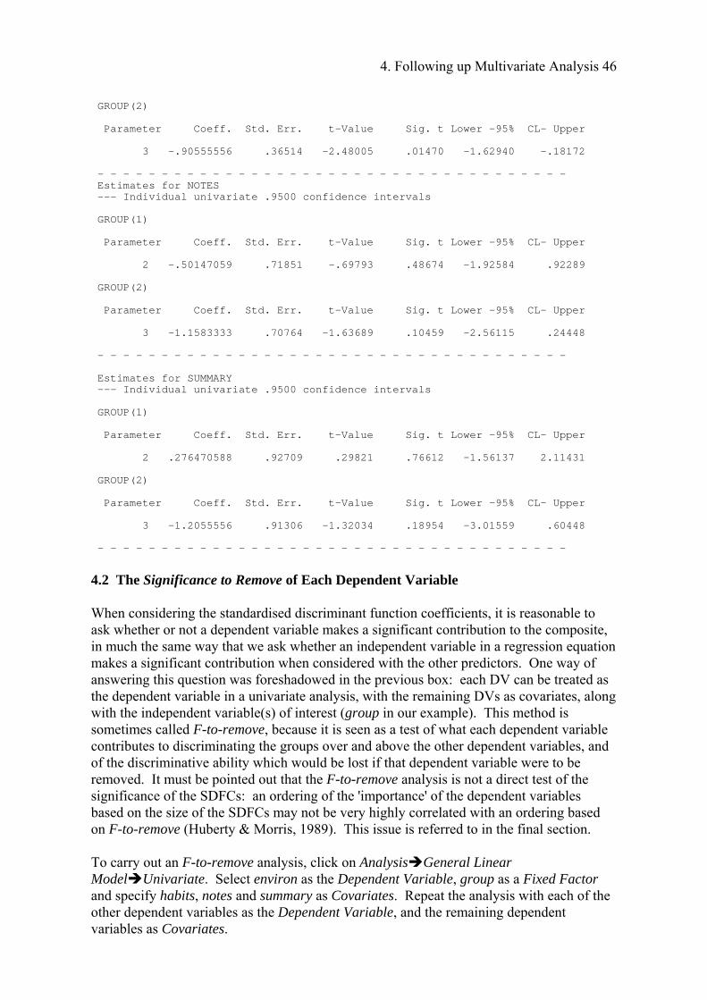
4. Following up Multivariate Analysis 46
GROUP(2) Parameter Coeff. Std. Err. t-Value Sig. t Lower -95% CL- Upper 3 -.90555556 .36514 -2.48005 .01470 -1.62940 -.18172 - - - - - - - - - - - - - - - - - - - - - - - - - - - - - - - - - - - - - Estimates for NOTES --- Individual univariate .9500 confidence intervals GROUP(1) Parameter Coeff. Std. Err. t-Value Sig. t Lower -95% CL- Upper 2 -.50147059 .71851 -.69793 .48674 -1.92584 .92289 GROUP(2) Parameter Coeff. Std. Err. t-Value Sig. t Lower -95% CL- Upper 3 -1.1583333 .70764 -1.63689 .10459 -2.56115 .24448 - - - - - - - - - - - - - - - - - - - - - - - - - - - - - - - - - - - - - Estimates for SUMMARY --- Individual univariate .9500 confidence intervals GROUP(1) Parameter Coeff. Std. Err. t-Value Sig. t Lower -95% CL- Upper 2 .276470588 .92709 .29821 .76612 -1.56137 2.11431 GROUP(2) Parameter Coeff. Std. Err. t-Value Sig. t Lower -95% CL- Upper 3 -1.2055556 .91306 -1.32034 .18954 -3.01559 .60448 - - - - - - - - - - - - - - - - - - - - - - - - - - - - - - - - - - - - -
4.2 The Significance to Remove of Each Dependent Variable When considering the standardised discriminant function coefficients, it is reasonable to ask whether or not a dependent variable makes a significant contribution to the composite, in much the same way that we ask whether an independent variable in a regression equation makes a significant contribution when considered with the other predictors. One way of answering this question was foreshadowed in the previous box: each DV can be treated as the dependent variable in a univariate analysis, with the remaining DVs as covariates, along with the independent variable(s) of interest (group in our example). This method is sometimes called F-to-remove, because it is seen as a test of what each dependent variable contributes to discriminating the groups over and above the other dependent variables, and of the discriminative ability which would be lost if that dependent variable were to be removed. It must be pointed out that the F-to-remove analysis is not a direct test of the significance of the SDFCs: an ordering of the 'importance' of the dependent variables based on the size of the SDFCs may not be very highly correlated with an ordering based on F-to-remove (Huberty & Morris, 1989). This issue is referred to in the final section. To carry out an F-to-remove analysis, click on AnalysisGeneral Linear ModelUnivariate. Select environ as the Dependent Variable, group as a Fixed Factor and specify habits, notes and summary as Covariates. Repeat the analysis with each of the other dependent variables as the Dependent Variable, and the remaining dependent variables as Covariates.
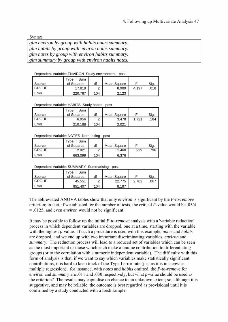
4. Following up Multivariate Analysis 47
Syntax glm environ by group with habits notes summary. glm habits by group with environ notes summary. glm notes by group with environ habits summary. glm summary by group with environ habits notes.
Dependent Variable: ENVIRON Study environment - post
17.818 2 8.909 4.197 .018
220.767 104 2.123
SourceGROUP
Error
Type III Sumof Squares df Mean Square F Sig.
Dependent Variable: HABITS Study habits - post
6.956 2 3.478 1.721 .184
210.188 104 2.021
SourceGROUP
Error
Type III Sumof Squares df Mean Square F Sig.
Dependent Variable: NOTES Note taking - post
2.921 2 1.460 .229 .796
663.099 104 6.376
SourceGROUP
Error
Type III Sumof Squares df Mean Square F Sig.
Dependent Variable: SUMMARY Summarising - post
45.551 2 22.775 2.782 .067
851.407 104 8.187
SourceGROUP
Error
Type III Sumof Squares df Mean Square F Sig.
The abbreviated ANOVA tables show that only environ is significant by the F-to-remove criterion; in fact, if we adjusted for the number of tests, the critical F-value would be .05/4 = .0125, and even environ would not be significant. It may be possible to follow up the initial F-to-remove analysis with a 'variable reduction' process in which dependent variables are dropped, one at a time, starting with the variable with the highest p-value. If such a procedure is used with this example, notes and habits are dropped, and we end up with two important discriminating variables, environ and summary. The reduction process will lead to a reduced set of variables which can be seen as the most important or those which each make a unique contribution to differentiating groups (or to the correlation with a numeric independent variable). The difficulty with this form of analysis is that, if we want to say which variables make statistically significant contributions, it is hard to keep track of the Type I error rate (just as it is in stepwise multiple regression); for instance, with notes and habits omitted, the F-to-remove for environ and summary are .011 and .030 respectively, but what p-value should be used as the criterion? The results may capitalise on chance to an unknown extent; so, although it is suggestive, and may be reliable, the outcome is best regarded as provisional until it is confirmed by a study conducted with a fresh sample.
4. Following up Multivariate Analysis 48
Huberty and Wisenbaker (1992) describe an approach to interpreting discriminant functions which involves grouping dependent variables into sets on the basis of F-to-remove results. For variables within a set, the F-to-remove values do not differ significantly, while they do differ significantly for variables in different sets. This method avoids some of the difficulties of controlling Type I error while facilitating meaningful interpretation of multivariate results, and allowing an ordering of the DVs in terms of their contribution to differentiating groups.
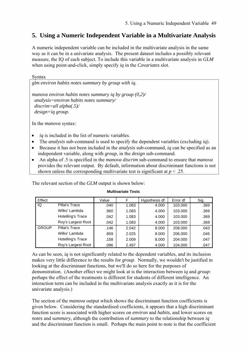
5. Using a Numeric Independent Variable 49
5. Using a Numeric Independent Variable in a Multivariate Analysis A numeric independent variable can be included in the multivariate analysis in the same way as it can be in a univariate analysis. The present dataset includes a possibly relevant measure, the IQ of each subject. To include this variable in a multivariate analysis in GLM when using point-and-click, simply specify iq in the Covariates slot. Syntax glm environ habits notes summary by group with iq. manova environ habits notes summary iq by group (0,2)/ analysis=environ habits notes summary/ discrim=all alpha(.5)/ design=iq group. In the manova syntax: iq is included in the list of numeric variables. The analysis sub-command is used to specify the dependent variables (excluding iq). Because it has not been included in the analysis sub-command, iq can be specified as an
independent variable, along with group, in the design sub-command. An alpha of .5 is specified in the manova discrim sub-command to ensure that manova
provides the relevant output. By default, information about discriminant functions is not shown unless the corresponding multivariate test is significant at p < .25.
The relevant section of the GLM output is shown below:
Multivariate Tests
.040 1.083 4.000 103.000 .369
.960 1.083 4.000 103.000 .369
.042 1.083 4.000 103.000 .369
.042 1.083 4.000 103.000 .369
.146 2.042 8.000 208.000 .043
.859 2.025 8.000 206.000 .045
.158 2.009 8.000 204.000 .047
.096 2.497 4.000 104.000 .047
Pillai's Trace
Wilks' Lambda
Hotelling's Trace
Roy's Largest Root
Pillai's Trace
Wilks' Lambda
Hotelling's Trace
Roy's Largest Root
EffectIQ
GROUP
Value F Hypothesis df Error df Sig.
As can be seen, iq is not significantly related to the dependent variables, and its inclusion makes very little difference to the results for group. Normally, we wouldn't be justified in looking at the discriminant functions, but we'll do so here for the purposes of demonstration. (Another effect we might look at is the interaction between iq and group: perhaps the effect of the treatments is different for students of different intelligence. An interaction term can be included in the multivariate analysis exactly as it is for the univariate analysis.) The section of the manova output which shows the discriminant function coefficients is given below. Considering the standardised coefficients, it appears that a high discriminant function score is associated with higher scores on environ and habits, and lower scores on notes and summary, although the contribution of summary to the relationship between iq and the discriminant function is small. Perhaps the main point to note is that the coefficient
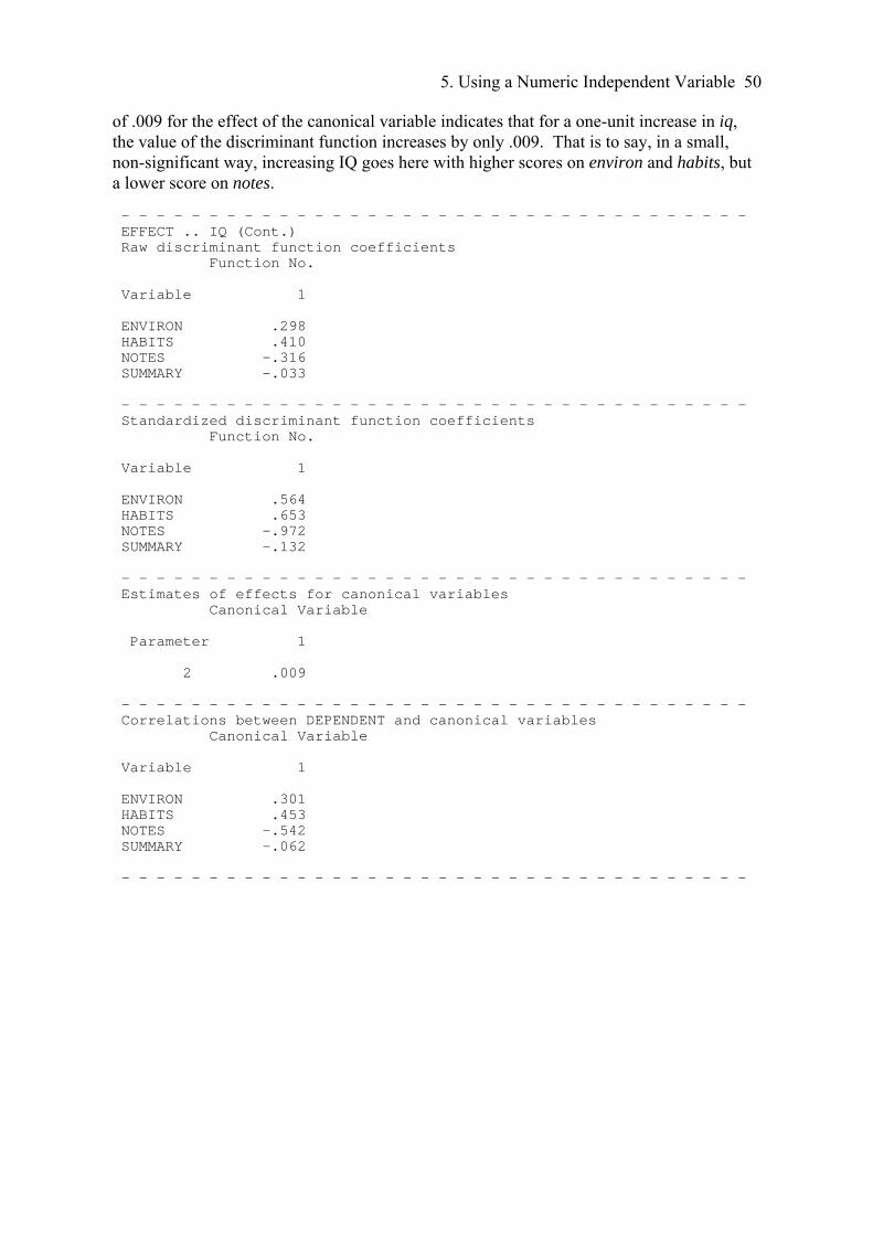
5. Using a Numeric Independent Variable 50
of .009 for the effect of the canonical variable indicates that for a one-unit increase in iq, the value of the discriminant function increases by only .009. That is to say, in a small, non-significant way, increasing IQ goes here with higher scores on environ and habits, but a lower score on notes. - - - - - - - - - - - - - - - - - - - - - - - - - - - - - - - - - - - - EFFECT .. IQ (Cont.) Raw discriminant function coefficients Function No. Variable 1 ENVIRON .298 HABITS .410 NOTES -.316 SUMMARY -.033 - - - - - - - - - - - - - - - - - - - - - - - - - - - - - - - - - - - - Standardized discriminant function coefficients Function No. Variable 1 ENVIRON .564 HABITS .653 NOTES -.972 SUMMARY -.132 - - - - - - - - - - - - - - - - - - - - - - - - - - - - - - - - - - - - Estimates of effects for canonical variables Canonical Variable Parameter 1 2 .009 - - - - - - - - - - - - - - - - - - - - - - - - - - - - - - - - - - - - Correlations between DEPENDENT and canonical variables Canonical Variable Variable 1 ENVIRON .301 HABITS .453 NOTES -.542 SUMMARY -.062 - - - - - - - - - - - - - - - - - - - - - - - - - - - - - - - - - - - -
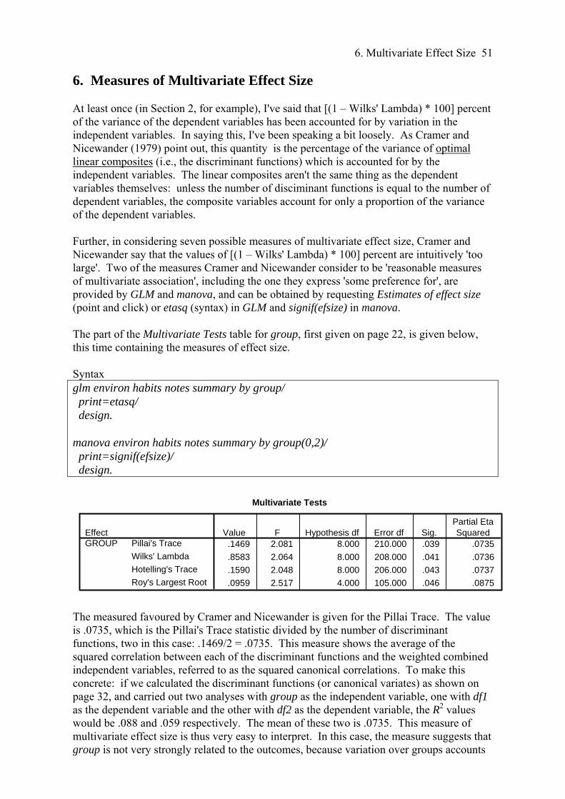
6. Multivariate Effect Size 51
6. Measures of Multivariate Effect Size At least once (in Section 2, for example), I've said that [(1 – Wilks' Lambda) * 100] percent of the variance of the dependent variables has been accounted for by variation in the independent variables. In saying this, I've been speaking a bit loosely. As Cramer and Nicewander (1979) point out, this quantity is the percentage of the variance of optimal linear composites (i.e., the discriminant functions) which is accounted for by the independent variables. The linear composites aren't the same thing as the dependent variables themselves: unless the number of disciminant functions is equal to the number of dependent variables, the composite variables account for only a proportion of the variance of the dependent variables. Further, in considering seven possible measures of multivariate effect size, Cramer and Nicewander say that the values of [(1 – Wilks' Lambda) * 100] percent are intuitively 'too large'. Two of the measures Cramer and Nicewander consider to be 'reasonable measures of multivariate association', including the one they express 'some preference for', are provided by GLM and manova, and can be obtained by requesting Estimates of effect size (point and click) or etasq (syntax) in GLM and signif(efsize) in manova. The part of the Multivariate Tests table for group, first given on page 22, is given below, this time containing the measures of effect size. Syntax glm environ habits notes summary by group/ print=etasq/ design. manova environ habits notes summary by group(0,2)/ print=signif(efsize)/ design.
Multivariate Tests
.1469 2.081 8.000 210.000 .039 .0735
.8583 2.064 8.000 208.000 .041 .0736
.1590 2.048 8.000 206.000 .043 .0737
.0959 2.517 4.000 105.000 .046 .0875
Pillai's Trace
Wilks' Lambda
Hotelling's Trace
Roy's Largest Root
EffectGROUP
Value F Hypothesis df Error df Sig.Partial EtaSquared
The measured favoured by Cramer and Nicewander is given for the Pillai Trace. The value is .0735, which is the Pillai's Trace statistic divided by the number of discriminant functions, two in this case: .1469/2 = .0735. This measure shows the average of the squared correlation between each of the discriminant functions and the weighted combined independent variables, referred to as the squared canonical correlations. To make this concrete: if we calculated the discriminant functions (or canonical variates) as shown on page 32, and carried out two analyses with group as the independent variable, one with df1 as the dependent variable and the other with df2 as the dependent variable, the R2 values would be .088 and .059 respectively. The mean of these two is .0735. This measure of multivariate effect size is thus very easy to interpret. In this case, the measure suggests that group is not very strongly related to the outcomes, because variation over groups accounts
6. Multivariate Effect Size 52
for only an average of the 7.35 % of the variation of each of the optimised discriminant functions. The second measure of effect size considered here is that associated with Wilks' Lambda in the above table, which is calculated as 1 – Λ 1/p, where Λ is Wilks' Lambda, and p is the number of discriminant functions. The value in this case is 1 - .85831/2 = .0736, the value shown in the table. This result is very similar to that for the first measure. A final point to note is that while these measures show the association between the independent variables and optimised linear composites of the dependent variables (rather than the variables themselves), they show the magnitude of the associations averaged over the discriminant functions, which means that they are not generally as large as the 'intuitively too large' Wilks' Lambda. For further discussion of measures of multivariate association, see Cramer and Nicewander (1979). Haase and Ellis (1987) give the formulae for other measures of multivariate association.
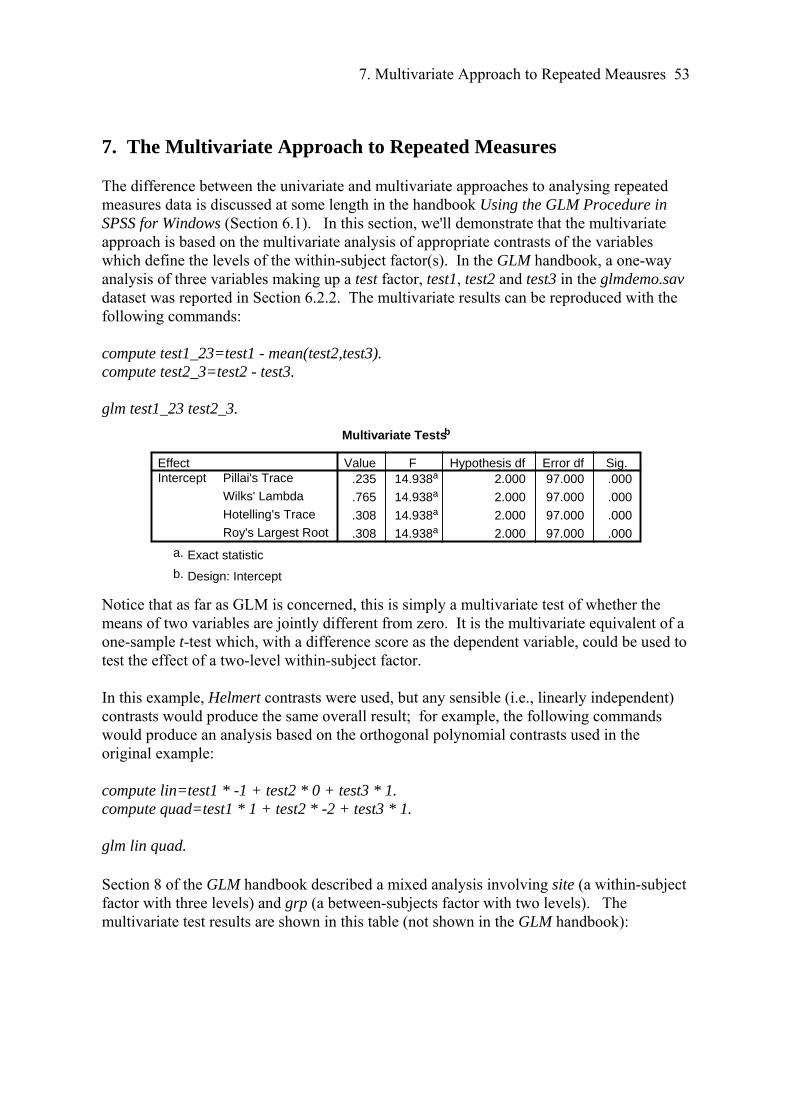
7. Multivariate Approach to Repeated Meausres 53
7. The Multivariate Approach to Repeated Measures The difference between the univariate and multivariate approaches to analysing repeated measures data is discussed at some length in the handbook Using the GLM Procedure in SPSS for Windows (Section 6.1). In this section, we'll demonstrate that the multivariate approach is based on the multivariate analysis of appropriate contrasts of the variables which define the levels of the within-subject factor(s). In the GLM handbook, a one-way analysis of three variables making up a test factor, test1, test2 and test3 in the glmdemo.sav dataset was reported in Section 6.2.2. The multivariate results can be reproduced with the following commands: compute test1_23=test1 - mean(test2,test3). compute test2_3=test2 - test3. glm test1_23 test2_3.
Multivariate Testsb
.235 14.938a 2.000 97.000 .000
.765 14.938a 2.000 97.000 .000
.308 14.938a 2.000 97.000 .000
.308 14.938a 2.000 97.000 .000
Pillai's Trace
Wilks' Lambda
Hotelling's Trace
Roy's Largest Root
EffectIntercept
Value F Hypothesis df Error df Sig.
Exact statistica.
Design: Interceptb.
Notice that as far as GLM is concerned, this is simply a multivariate test of whether the means of two variables are jointly different from zero. It is the multivariate equivalent of a one-sample t-test which, with a difference score as the dependent variable, could be used to test the effect of a two-level within-subject factor. In this example, Helmert contrasts were used, but any sensible (i.e., linearly independent) contrasts would produce the same overall result; for example, the following commands would produce an analysis based on the orthogonal polynomial contrasts used in the original example: compute lin=test1 * -1 + test2 * 0 + test3 * 1. compute quad=test1 * 1 + test2 * -2 + test3 * 1. glm lin quad. Section 8 of the GLM handbook described a mixed analysis involving site (a within-subject factor with three levels) and grp (a between-subjects factor with two levels). The multivariate test results are shown in this table (not shown in the GLM handbook):

7. Multivariate Approach to Repeated Meausres 54
Multivariate Testsb
.542 56.803a 2.000 96.000 .000
.458 56.803a 2.000 96.000 .000
1.183 56.803a 2.000 96.000 .000
1.183 56.803a 2.000 96.000 .000
.057 2.907a 2.000 96.000 .059
.943 2.907a 2.000 96.000 .059
.061 2.907a 2.000 96.000 .059
.061 2.907a 2.000 96.000 .059
Pillai's Trace
Wilks' Lambda
Hotelling's Trace
Roy's Largest Root
Pillai's Trace
Wilks' Lambda
Hotelling's Trace
Roy's Largest Root
EffectSITE
SITE * GRP
Value F Hypothesis df Error df Sig.
Exact statistica.
Design: Intercept+GRP Within Subjects Design: SITE
b.
Using difference contrasts, this result can be reproduced with these commands: compute site2_1=site2 - site1. compute site3_12=site3 - mean(site1,site2). glm site2_1 site3_12 by grp. The results are as follows:
Multivariate Testsb
.542 56.803a 2.000 96.000 .000
.458 56.803a 2.000 96.000 .000
1.183 56.803a 2.000 96.000 .000
1.183 56.803a 2.000 96.000 .000
.057 2.907a 2.000 96.000 .059
.943 2.907a 2.000 96.000 .059
.061 2.907a 2.000 96.000 .059
.061 2.907a 2.000 96.000 .059
Pillai's Trace
Wilks' Lambda
Hotelling's Trace
Roy's Largest Root
Pillai's Trace
Wilks' Lambda
Hotelling's Trace
Roy's Largest Root
EffectIntercept
GRP
Value F Hypothesis df Error df Sig.
Exact statistica.
Design: Intercept+GRPb.
Notice that, as in the first example, the multivariate test of the intercept is equivalent to the test of the site factor; also, as far as GLM is concerned, there is no interaction, just a multivariate test of grp. This is the multivariate equivalent of an independent t-test with difference scores as the dependent variable. 7.1 Profile Analysis
A profile analysis is like a repeated measures analysis, but does't have a within-subject factor. Imagine that you have a number of variables all measured on the same scale (i.e., commensurate variables), such as a set of personality scales all based on the average of responses made to individual items using the same 7-point scale. Say there are five scales, Introversion, Extraversion, Neuroticism, Ruthlessness and Authoritarianism: IENRA for short. We could use them to define a within-subject factor called scale, for example, but that's not really appropriate and it's not what we're interested in. What we really want to

7. Multivariate Approach to Repeated Meausres 55
know is whether the profile of means differs over two or more groups of subjects and, failing that, whether the average over the five scales differs over the groups. Profile analysis is similar to repeated measures analysis in that the dependent variables are not the variables themselves but some set of differences between them; for example, the dependent variables for a profile analysis of the I, E, N, R and A variables above could be created as follows: compute I_E = I – E. compute E_N = E – N. compute N_R = N – R. compute R_A = R – A i.e., by obtaining the difference between each pair of neighbouring variables. Assuming that the grouping variable is called group, the profile analysis could be carried out with this syntax (or the equivalent point-and-click): glm i_e e_n n_r r_a by group. If there is a significant group effect, it means that the pattern of differences differs over groups, i.e., that the profile is different for the two groups. The actual nature of the differences may be investigated with further analyses, such as paired t-tests. If there is no group effect, it means that the profiles aren't very different, but still leaves the possibility that there are level differences between the groups. This possibility could be tested by using the mean of the five original variables as the dependent variable in a univariate analysis. For example compute ienra = mean(i,e,n,r,a). glm ienra by group. With the manova procedure, it's possible to do all of the above using one set of commands: manova 1 e n r a by group(1,2)/ transform=repeated/ rename= av i_e e_n n_r r_a/ analysis=(av/ i_e e_n n_r r_a)/ design. The transform sub-command does the same sort of job as the contrast sub-command, but can be used when there is no within-subjects factor. The repeated keyword asks for the analysis to be performed on the differences between neighbouring variables. The first variable created by the repeated transformation is the average of all five of the variables. The rename sub-command is cosmetic and simply supplies labels for the transformed variables; it is optional and, if it had not been used, the variables would have been named t1 to t5, with t1 being the average of all five of the original variables and t2 to t5 being the differences between neighbouring variables. Another feature of manova is shown in the analysis sub-command, which asks for two separate analyses, the first based on the average of the variables, and the second based on the differences.

7. Multivariate Approach to Repeated Meausres 56
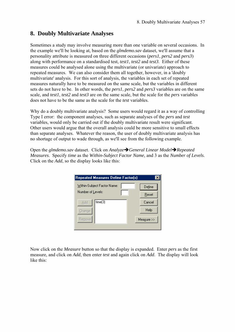
8. Doubly Multivariate Analyses 57
8. Doubly Multivariate Analyses Sometimes a study may involve measuring more than one variable on several occasions. In the example we'll be looking at, based on the glmdemo.sav dataset, we'll assume that a personality attribute is measured on three different occasions (pers1, pers2 and pers3) along with performance on a standardised test, test1, test2 and test3. Either of these measures could be analysed alone using the multivariate (or univariate) approach to repeated measures. We can also consider them all together, however, in a 'doubly multivariate' analysis. For this sort of analysis, the variables in each set of repeated measures naturally have to be measured on the same scale, but the variables in different sets do not have to be. In other words, the pers1, pers2 and pers3 variables are on the same scale, and test1, test2 and test3 are on the same scale, but the scale for the pers variables does not have to be the same as the scale for the test variables. Why do a doubly multivariate analysis? Some users would regard it as a way of controlling Type I error: the component analyses, such as separate analyses of the pers and test variables, would only be carried out if the doubly multivariate result were significant. Other users would argue that the overall analysis could be more sensitive to small effects than separate analyses. Whatever the reason, the user of doubly multivariate analysis has no shortage of output to wade through, as we'll see from the following example. Open the glmdemo.sav dataset. Click on AnalyzeGeneral Linear ModelRepeated Measures. Specify time as the Within-Subject Factor Name, and 3 as the Number of Levels. Click on the Add, so the display looks like this: Now click on the Measure button so that the display is expanded. Enter pers as the first measure, and click on Add, then enter test and again click on Add. The display will look like this:
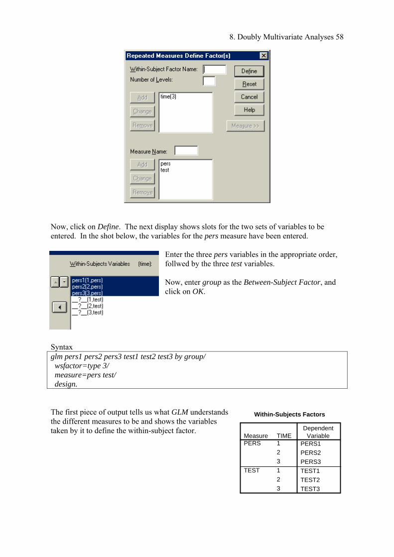
8. Doubly Multivariate Analyses 58
Within-Subjects Factors
PERS1
PERS2
PERS3
TEST1
TEST2
TEST3
TIME1
2
3
1
2
3
MeasurePERS
TEST
DependentVariable
Now, click on Define. The next display shows slots for the two sets of variables to be entered. In the shot below, the variables for the pers measure have been entered.
Enter the three pers variables in the appropriate order, follwed by the three test variables. Now, enter group as the Between-Subject Factor, and click on OK.
Syntax glm pers1 pers2 pers3 test1 test2 test3 by group/ wsfactor=type 3/ measure=pers test/ design. The first piece of output tells us what GLM understands the different measures to be and shows the variables taken by it to define the within-subject factor.
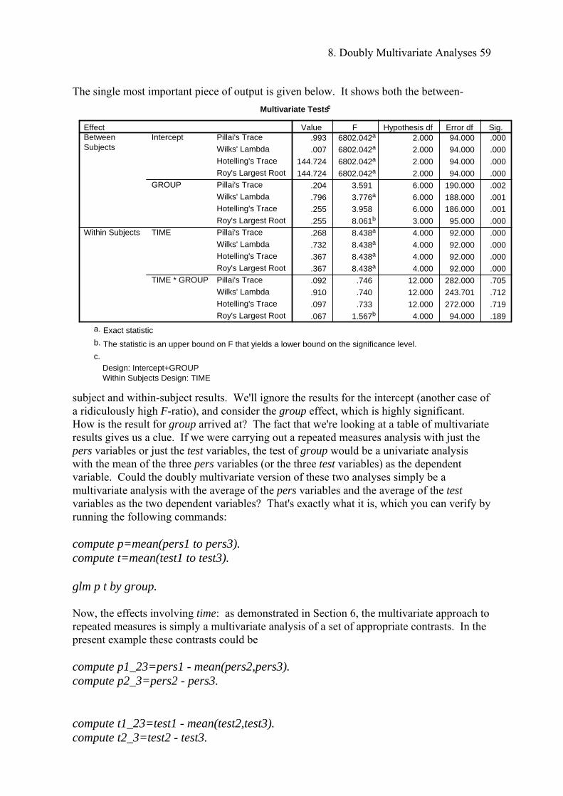
8. Doubly Multivariate Analyses 59
The single most important piece of output is given below. It shows both the between-
Multivariate Testsc
.993 6802.042a 2.000 94.000 .000
.007 6802.042a 2.000 94.000 .000
144.724 6802.042a 2.000 94.000 .000
144.724 6802.042a 2.000 94.000 .000
.204 3.591 6.000 190.000 .002
.796 3.776a 6.000 188.000 .001
.255 3.958 6.000 186.000 .001
.255 8.061b 3.000 95.000 .000
.268 8.438a 4.000 92.000 .000
.732 8.438a 4.000 92.000 .000
.367 8.438a 4.000 92.000 .000
.367 8.438a 4.000 92.000 .000
.092 .746 12.000 282.000 .705
.910 .740 12.000 243.701 .712
.097 .733 12.000 272.000 .719
.067 1.567b 4.000 94.000 .189
Pillai's Trace
Wilks' Lambda
Hotelling's Trace
Roy's Largest Root
Pillai's Trace
Wilks' Lambda
Hotelling's Trace
Roy's Largest Root
Pillai's Trace
Wilks' Lambda
Hotelling's Trace
Roy's Largest Root
Pillai's Trace
Wilks' Lambda
Hotelling's Trace
Roy's Largest Root
EffectIntercept
GROUP
BetweenSubjects
TIME
TIME * GROUP
Within Subjects
Value F Hypothesis df Error df Sig.
Exact statistica.
The statistic is an upper bound on F that yields a lower bound on the significance level.b.
Design: Intercept+GROUP Within Subjects Design: TIME
c.
subject and within-subject results. We'll ignore the results for the intercept (another case of a ridiculously high F-ratio), and consider the group effect, which is highly significant. How is the result for group arrived at? The fact that we're looking at a table of multivariate results gives us a clue. If we were carrying out a repeated measures analysis with just the pers variables or just the test variables, the test of group would be a univariate analysis with the mean of the three pers variables (or the three test variables) as the dependent variable. Could the doubly multivariate version of these two analyses simply be a multivariate analysis with the average of the pers variables and the average of the test variables as the two dependent variables? That's exactly what it is, which you can verify by running the following commands: compute p=mean(pers1 to pers3). compute t=mean(test1 to test3). glm p t by group. Now, the effects involving time: as demonstrated in Section 6, the multivariate approach to repeated measures is simply a multivariate analysis of a set of appropriate contrasts. In the present example these contrasts could be compute p1_23=pers1 - mean(pers2,pers3). compute p2_3=pers2 - pers3. compute t1_23=test1 - mean(test2,test3). compute t2_3=test2 - test3.
8. Doubly Multivariate Analyses 60
for pers and test respectively. As you will have anticipated, in doubly multivariate analyses the sets of contrasts for all of the variables involved are entered as dependent variables. Again, you can verify that this is the case by running the following commands (Helmert contrasts are used here, but you can use any other sensible contrasts): compute p1_23=pers1 - mean(pers2,pers3). compute p2_3=pers2 - pers3. compute t1_23=test1 - mean(test2,test3). compute t2_3=test2 - test3. glm p1_23 p2_3 t1_23 t2_3 by group. As the results of this analysis, and those in the original table, show, there are clear effects for group and time, but no suggestion of a group by time interaction. Now, looking at the rest of the output, we find a table with large heading, Tests of Within-Subjects Effects, the title Multivariate and a footnote saying Tests are based on averaged values. This table shows the results for what might be called 'the univariate approach to doubly multivariate analysis'. Because this handbook is concerned with multivariate analyses, we won't consider this table further. Similarly, the next table, headed Univariate Tests, contains the results for repeated measures analyses carried out separately for the pers and test variables, based on the univariate approach to repeated measures. GLM doesn't print out results for separate multivariate analyses of the pers and time variables. The remaining tables (not given here) show the within-subject contrasts, and the between-subject effects, separately for each set of variables. It's interesting to note that while there is a clearly significant group effect for pers, the comparable effect for test is marginal (p = .055). Finally, it's worth noting that if a plot with time on the horizontal axis and with separate lines for group is specified as part of the multivariate analysis, GLM sensibly does a separate graph for pers and test.
9. Issues and Further Reading 61
9. Some Issues and Further Reading 9.1 Univariate or Multivariate? If you have a number of dependent variables and are intending to carry out the same analysis with each of them, you have the choice of performing a number of univariate analyses or a smaller number of multivariate analyses (perhaps just one). Huberty (1994), Huberty & Morris (1989) and Haase & Ellis (1987) discuss this issue. The general opinion is that a multivariate analysis is particularly appropriate if the analyst is interested in how variables combine to differentiate groups (or correlate with a numeric independent variable) and in the contribution of each variable to the discrimination. These two things will generally only be of interest if the dependent variables are correlated. Coming from the other direction, an analyst may hesitate to carry out multiple univariate analyses when the dependent variables are correlated, even if there is no interest in the way the variables fit together to make a dimension, because of the overlap and lack of independence involved. In this case, a mutivariate analysis may be carried out to take the correlations into account and to avoid redundancy. Although some writers suggest that multivariate analysis may control Type I and Type II error (e.g., Haase & Ellis, 1987), others argue that control of Type I error is not a sufficient reason for performing a multivariate analysis: if that is the main goal, a Bonferroni adjustment can be used to take the number of analyses into account (e.g., Huberty & Morris, 1989). 9.2 Following up a Significant Multivariate Result A question related to the previous one concerns the best way to follow up a significant MANOVA result, especially in terms of examination of the dependent variables. A number of writers (e.g., Share, 1984) have poured scorn on users who simply follow up a significant multivariate result with separate univariate analyses. These writers argue that univariate analyses ignore the information about the effects of the correlations of the dependent variables which has been provided by the multivariate result. When a series of univariate analyses is performed after a multivariate analysis, it is fair to ask why the analyst has gone to the trouble of performing the MANOVA in the first place. A number of writers (e.g., Spector, 1977; Wilkinson, 1975) have considered various ways of using the multivariate results – namely, the standardised discriminant function coefficients and the correlations of the dependent variables with the discriminant function(s) [sometimes called structure coefficients], along with results of univariate analyses -- to interpret the results of multivariate analyses. It is tempting to base interpretation on the standardised discriminant function coefficients (SDFCs), and to consider that the variables with the largest SDFCs are the most important, in some sense. As various writers (e.g., Huberty & Morris, 1989; Sharma, 1996) have pointed out, however, the values of the SDFCs may fluctuate greatly from sample to sample, especially when the dependent variables are highly correlated and the samples are small. Huberty & Morris (1989) further point out that the sampling variability of SDFCs is not considered; i.e., there is no significance test for the SDFCs. These writers prefer to use F-to-remove values to order the contribution of dependent variables to the composite (Section 4.2) and, as mentioned previously, Huberty and Wisenbaker (1992) suggest using F-to-remove values to group dependent variables into homogeneous subsets. As also
9. Issues and Further Reading 62
mentioned earlier, the ordering of variables on the basis of F-to-remove values may not correlate very highly with an ordering based on the size of the SDFCs (Huberty & Morris, 1989). Some writers (e.g., Sharma, 1996) suggest using the correlations between the dependent variables and the discriminant functions (structure coefficients) to label the discriminant functions and "also for interpreting the contribution of each variable to the formation of the discriminant function" (p. 254). In fact, the SDFC for a variable may show that it makes very little contribution to a discriminant function despite being highly correlated with it. Furthermore, Huberty (1972) has shown that, with two groups, the squared structural coefficients are proportional to the corresponding univariate F-values, so that, although the structural coefficients may be useful for labelling a discriminant function, they do not contribute any truly multivariate information to deciding on the relative importance of dependent variables. In summary, there are drawbacks to any approach to interpreting the result of multivariate analyses which depends on only one source of information, and I agree with the advice of Hair et al (1995) that "… the analyst should employ all available methods to arrive at the most accurate interpretation" (p. 209). It also pays to keep an eye out for articles such as that by Thomas (1992), which propose new ways of interpreting discriminant functions. 9.3 Power Stevens (1980, 1986) discusses power with respect to multivariate designs and provides tables which allow researchers to estimate power for different numbers of groups, group sizes and numbers of dependent variables. Researchers who do not have easy access to power programs may use a method described by D'Amico, Neilands & Zambarno (2001), which is based on the SPSS manova procedure, and takes advantage of the fact that manova can both write out and read in data in matrix form (which GLM is not able to do). The method will be described with the data in ck.sav. The manova commands to save the data in matrix form are: manova environ habits notes summary by group(0,2)/ matrix=out(*)/ design. The matrix subcommand instructs manova to write the data out in matrix form, replacing the original data in the Data Window. The data are shown below:
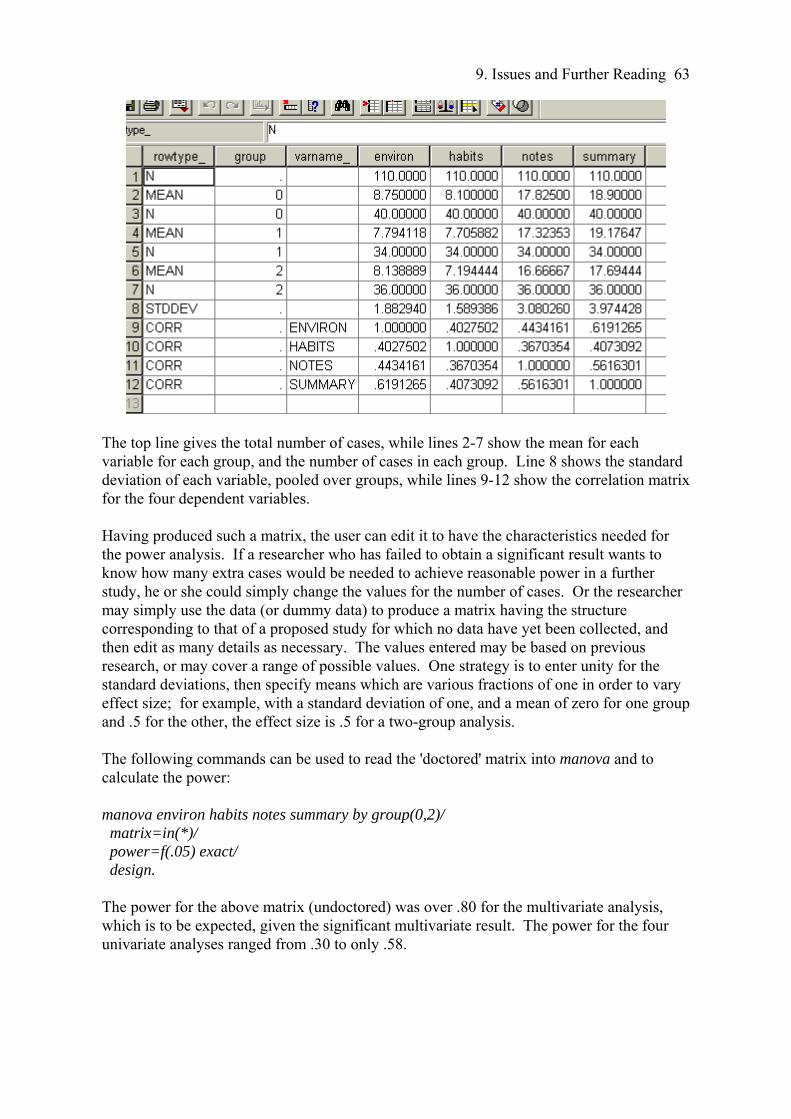
9. Issues and Further Reading 63
The top line gives the total number of cases, while lines 2-7 show the mean for each variable for each group, and the number of cases in each group. Line 8 shows the standard deviation of each variable, pooled over groups, while lines 9-12 show the correlation matrix for the four dependent variables. Having produced such a matrix, the user can edit it to have the characteristics needed for the power analysis. If a researcher who has failed to obtain a significant result wants to know how many extra cases would be needed to achieve reasonable power in a further study, he or she could simply change the values for the number of cases. Or the researcher may simply use the data (or dummy data) to produce a matrix having the structure corresponding to that of a proposed study for which no data have yet been collected, and then edit as many details as necessary. The values entered may be based on previous research, or may cover a range of possible values. One strategy is to enter unity for the standard deviations, then specify means which are various fractions of one in order to vary effect size; for example, with a standard deviation of one, and a mean of zero for one group and .5 for the other, the effect size is .5 for a two-group analysis. The following commands can be used to read the 'doctored' matrix into manova and to calculate the power: manova environ habits notes summary by group(0,2)/ matrix=in(*)/ power=f(.05) exact/ design. The power for the above matrix (undoctored) was over .80 for the multivariate analysis, which is to be expected, given the significant multivariate result. The power for the four univariate analyses ranged from .30 to only .58.
References 64
References Bray, J. & Maxwell, S. (1985). Multivariate analysis of variance. Beverly Hills: Sage. [HA29.Q35] Cramer, E., & Nicewander, W. (1979). Some symmetric, invariant measures of multivariate association. Psychometrika, 44, 43-54. D'Amico, E., Neilands, T., & Zambarano, R. (2001). Power designs for multivariate and repeated measures designs: A flexible approach using the SPSS MANOVA procedure. Behavior Research Methods, Instruments, & Computers, 33, 479-484. Goldstein, R. (1991). Test for multivariate normality. Stata Technical Bulletin Reprints, 1, 175. Haase, R. & Ellis, M. (1987). Multivariate analysis of variance. Journal of Counselling Psychology, 34, (4), 404-413. Hair, J. et.al. , (1995). Multivariate data analysis with readings (Fourth Edition) Englewood Cliffs, NJ: Prentice-Hall. [QA278.M85] Huberty, C. (1994). Why multivariable analyses? Educational and Psychological Measurement, 54, 620-627. Huberty, C.J. & Morris, J.D. (1989). Multivariate analysis versus multiple univariate analyses. Psychological Bulletin, 105, 302-308. Huberty, C.J. & Smith, J.D. (1982). The study of effects in MANOVA. Multivariate Behavioural Research, 17, 417-432. Huberty, C.J. & Wisenbaker, J. M. (1992). Variable importance in multivariate group comparisons. Journal of Educational Statistics, 17, 75-91. Sharma, S. (1996). Applied multivariate techniques. NY: Wiley. [QA278.S485] Share, D. (1984). Interpreting the output of multivariate analyses: A discussion of current approaches. British Journal of Psychology, 75, 349-362. Spector, P. (1977). What to do with significant multivariate effects in multivariate analyses of variance. Journal of Applied Psychology, 67, 158-163. Stevens, J. (1980). Power of the multivariate analysis of variance tests. Psychological Bulletin, 1980, 88, 728-737. Stevens, J. (1986). Applied multivariate statistics for the social sciences. Hillsdale, N.J.: Lawrence Erlbaum. [This is the 1st edition; the book is now up to the 4th edition. The Macquarie library has the 3rd edition at QA 278.S74] Tacq, J. (1997). Multivariate analysis techniques in social science research. London: Sage. Thomas, D. (1992). Interpreting discriminant functions: A data analytic approach. Multivariate Behavioral Research, 27, 335-362. Thompson, B. (1990). MULTINOR: A Fortran Program that Assists in Evaluating Multi-variate Normality. Educational and Psychological Measurement, 50, 845-848. Wilkinson, L. (1975). Response variable hypotheses in the multivariate analysis of variance. Psychological Bulletin, 82, 408-412.
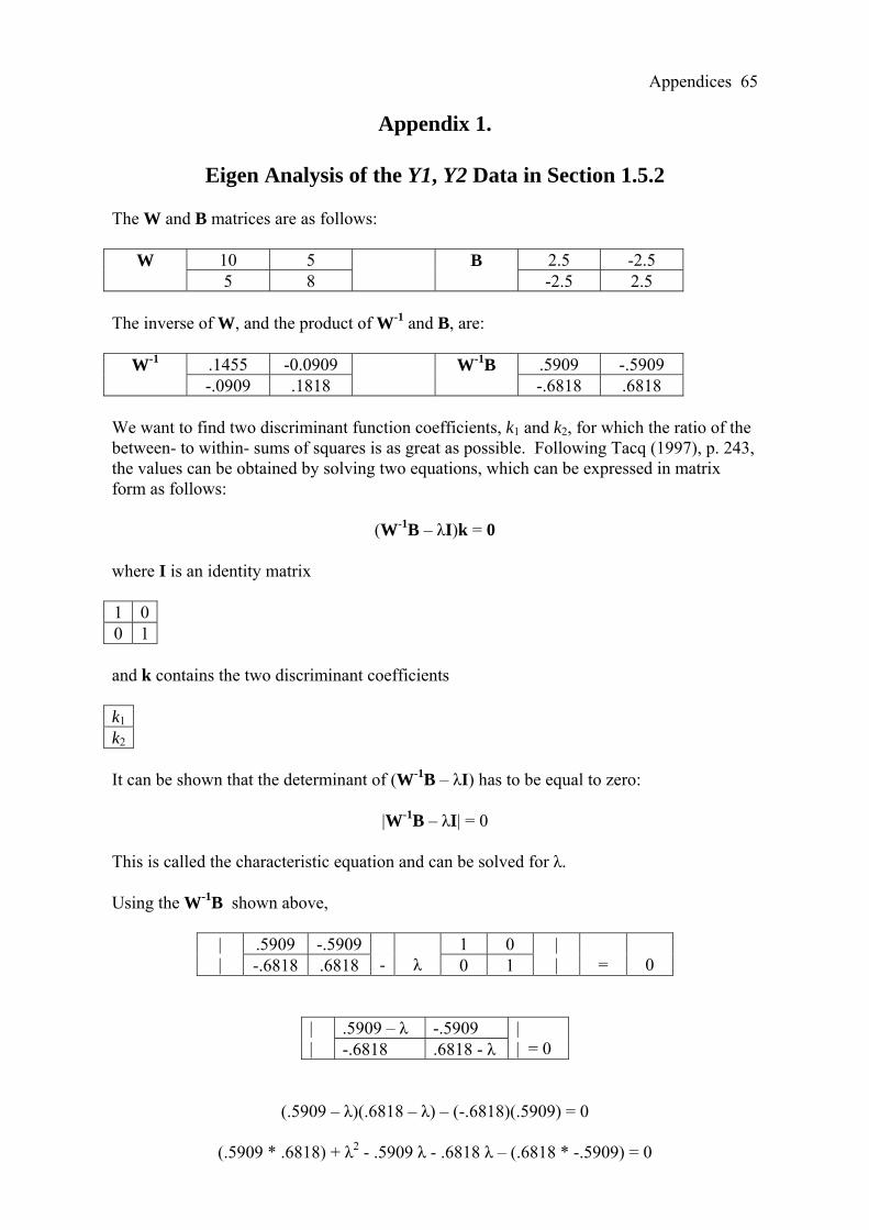
Appendices 65
Appendix 1.
Eigen Analysis of the Y1, Y2 Data in Section 1.5.2 The W and B matrices are as follows:
10 5 2.5 -2.5 W 5 8
B -2.5 2.5
The inverse of W, and the product of W-1 and B, are:
.1455 -0.0909 .5909 -.5909 W-1 -.0909 .1818
W-1B -.6818 .6818
We want to find two discriminant function coefficients, k1 and k2, for which the ratio of the between- to within- sums of squares is as great as possible. Following Tacq (1997), p. 243, the values can be obtained by solving two equations, which can be expressed in matrix form as follows:
(W-1B – λI)k = 0 where I is an identity matrix 1 0 0 1 and k contains the two discriminant coefficients k1
k2
It can be shown that the determinant of (W-1B – λI) has to be equal to zero:
|W-1B – λI| = 0 This is called the characteristic equation and can be solved for λ. Using the W-1B shown above,
.5909 -.5909 1 0 | | -.6818 .6818
-
λ 0 1
| |
=
0
.5909 – λ -.5909 | | -.6818 .6818 - λ
| | = 0
(.5909 – λ)(.6818 – λ) – (-.6818)(.5909) = 0
(.5909 * .6818) + λ2 - .5909 λ - .6818 λ – (.6818 * -.5909) = 0
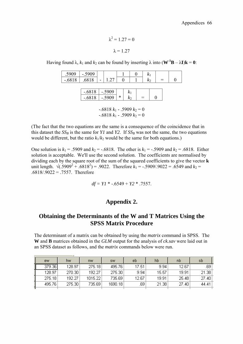
Appendices 66
λ2 = 1.27 = 0
λ = 1.27
Having found λ, k1 and k2 can be found by inserting λ into (W-1B – λI)k = 0:
.5909 -.5909 1 0 -.6818 .6818
-
1.27 0 1
k1
k2
=
0
-.6818 -.5909-.6818 -.5909
*
k1
k2
=
0
-.6818 k1 - .5909 k2 = 0 -.6818 k1 - .5909 k2 = 0
(The fact that the two equations are the same is a consequence of the coincidence that in this dataset the SSB is the same for Y1 and Y2. If SSB was not the same, the two equations would be different, but the ratio k1/k2 would be the same for both equations.) One solution is k1 = .5909 and k2 = -.6818. The other is k1 = -.5909 and k2 = .6818. Either solution is acceptable. We'll use the second solution. The coefficients are normalised by dividing each by the square root of the sum of the squared coefficients to give the vector k unit length. √(.59092 + .68182) = .9022. Therefore k1 = -.5909/.9022 = .6549 and k2 = .6818/.9022 = .7557. Therefore
df = Y1 * -.6549 + Y2 * .7557.
Appendix 2.
Obtaining the Determinants of the W and T Matrices Using the SPSS Matrix Procedure
The determinant of a matrix can be obtained by using the matrix command in SPSS. The W and B matrices obtained in the GLM output for the analysis of ck.sav were laid out in an SPSS dataset as follows, and the matrix commands below were run.
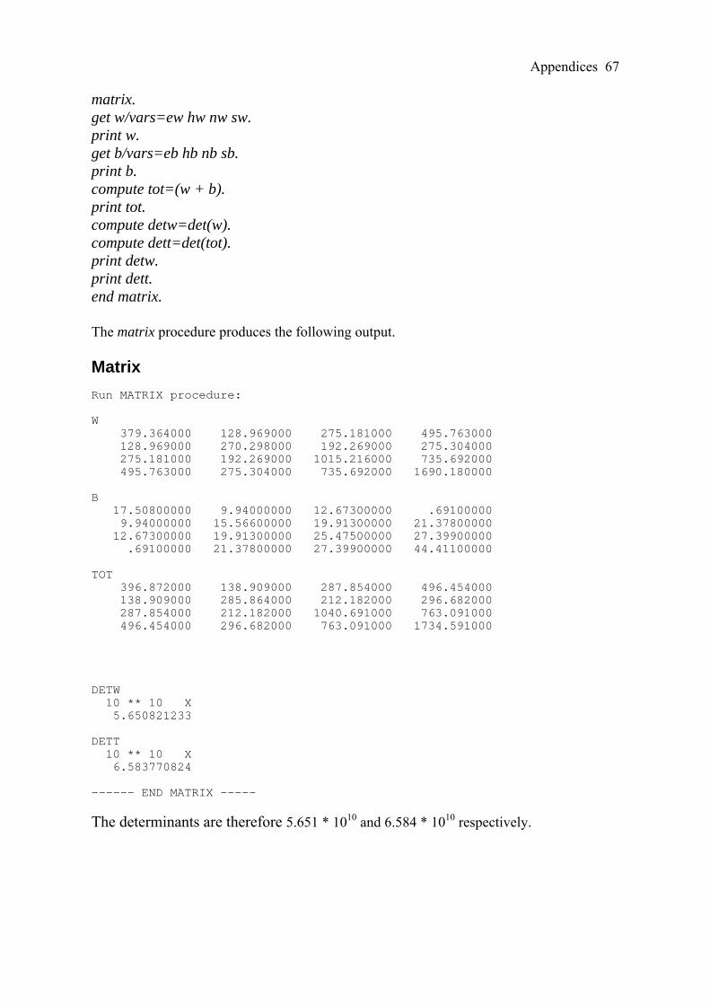
Appendices 67
matrix. get w/vars=ew hw nw sw. print w. get b/vars=eb hb nb sb. print b. compute tot=(w + b). print tot. compute detw=det(w). compute dett=det(tot). print detw. print dett. end matrix. The matrix procedure produces the following output. Matrix Run MATRIX procedure: W 379.364000 128.969000 275.181000 495.763000 128.969000 270.298000 192.269000 275.304000 275.181000 192.269000 1015.216000 735.692000 495.763000 275.304000 735.692000 1690.180000 B 17.50800000 9.94000000 12.67300000 .69100000 9.94000000 15.56600000 19.91300000 21.37800000 12.67300000 19.91300000 25.47500000 27.39900000 .69100000 21.37800000 27.39900000 44.41100000 TOT 396.872000 138.909000 287.854000 496.454000 138.909000 285.864000 212.182000 296.682000 287.854000 212.182000 1040.691000 763.091000 496.454000 296.682000 763.091000 1734.591000 DETW 10 ** 10 X 5.650821233 DETT 10 ** 10 X 6.583770824 ------ END MATRIX -----
The determinants are therefore 5.651 * 1010 and 6.584 * 1010 respectively.