Embed Size (px)
Citation preview
Multivariate Demand: Modeling and Estimation from
Censored Sales
Catalina Stefanescu∗
Abstract
Demand modeling and forecasting is important for inventory management, retail
assortment and revenue management applications. Current practice focuses on univari-
ate demand forecasting, where models are built separately for each product. However,
in many industries there is empirical evidence of correlated product demand. In ad-
dition, demand is usually observed in several periods during a selling horizon, and it
may be truncated due to inventory constraints so that in practice only censored sales
data are recorded. Ignoring the inter-product demand correlation or the serial corre-
lation of demand from one selling period to the next leads to biased and inefficient
estimates of the true demand distributions. In this paper we propose a class of models
for multi-product multiperiod aggregate demand forecasting. We develop an approach
for estimating the parameters of the demand models from censored sales data in a
maximum likelihood framework using the Expectation-Maximization (EM) algorithm.
Through a simulation study, we show that the algorithm is computationally attractive
and leads to maximum likelihood estimates with good properties, under different de-
mand and censoring scenarios. We exemplify the methodology with the analysis of two
booking data sets from the entertainment and the airline industries, and show that the
use of these models in a revenue management setting for airlines increases the revenue
by up to 11% relative to the use of alternative demand forecasting methods.
Key words: Demand estimation; multivariate models; maximum likelihood; EM algo-
rithm; revenue management; retailing; inventory management.
∗Management Science and Operations, London Business School, London NW14SA, United Kingdom.Email: [email protected].
1
1 Introduction
Modeling and forecasting of customer demand is crucial in many application areas, including
revenue management, retail assortment, and inventory management. In revenue management
systems, demand forecasts are needed as inputs to any price optimization module (van
Ryzin 2005), and sources from the airline industry estimate that a 20% reduction in demand
forecast error may translate into a 1% increase in revenues (Talluri and van Ryzin 2003); in
competitive industries with thin margins, such as airlines, a 1% improvement in revenues can
be the difference between a successful and an unsustainable business. In retailing, knowledge
of the true demand distribution and substitution rates is important for a wide range of
category management decisions, such as the ideal assortment to carry, the optimal inventory
to be stocked from each item, and the stock replenishment rates. Inventory management
systems rely on accurate methods for estimating customer demand (Agrawal and Smith
1996), and their efficiency is particularly important for products (such as basic merchandise)
where retailers have had increased competitive pressure.
There are two major challenges in modeling and forecasting customer demand. The first
issue is that in practice different demand streams are often correlated, and demand models
must account for this correlation. Patterns of demand correlation occur along two dimensions
— the time dimension and the product dimension. Both types of demand correlation have
been empirically documented in many industries, and they often arise in the same context.
The time dimension of demand correlation occurs when a firm sells products during
a time horizon over which demand for a product recorded in different periods is related.
For example, this is the case of travel tickets (e.g., train or airlines) sold during a booking
period; tickets for travel during holiday times will be in higher demand throughout the
booking horizon. In retailing, where cyclical demand fluctuations due to promotions occur
commonly, inventory management decisions are often made periodically, hence there is a
need for multi-period models that account for the serial correlation of demand from one
period to the next.
The product dimension of demand correlation occurs when demand for different but
related products is dependent. In magazine retailing, for example, Koschat (2008) finds
evidence that demand for different magazines is correlated, and that a change in inventory
levels of one magazine affects sales of the others. Correlation of product demands sometimes
arises due to customer behavior. In retailing, correlated demand for color or style varieties
of trendy apparel is a result of trend-following behavior. In general, when the retailer offers
different styles, colors or flavors of the same product, substitution by the customer is likely
2
to lead to correlated demands. Other instances of substitution which may induce demand
correlation include buy-up (e.g., buying a higher fare ticket when the lower fares are not
available) and buy-down (e.g., buying a lower fare ticket instead of a higher fare when the
seller offers discounts). Note, however, that product demand correlation may happen not
just due to substitution effects and other features of customer behavior, but also because
products share some common characteristics. For example, demand for airline tickets on
the London – New York route is likely to be high both in economy class and in business
class, not primarily because of customer substitution (the high price difference will usually
preclude this) but mainly since the two cities are both tourist and business destinations.
The second major issue in modeling and forecasting customer demand is estimating the
parameters of demand models from censored sales data. In practice, only the recorded
product sales are often available for estimation. However, actual demand may be greater
than observed sales when a product sells out, hence sales data are just censored rather
than exact observations of demand. Unobservable lost sales are prevalent in retailing where
unmet demand arises when products are out-of-stock, particularly for low-cost, nondurable
merchandise. If customers encounter a stockout for the product they desire, they may
substitute with another product, place an order for delivery in the future, or move on without
recording their request.1 In the latter case, the sales data for the desired product are censored
observations of demand.
Demand predictions based on sales data without accounting for the stockout effect poten-
tially lead to two types of error. First, the forecasts for stocked-out products are negatively
biased and the extent of the bias depends on the stockout incidence frequency. Wecker
(1978) shows that stockouts also affect the estimate of the forecast error variance, and that
the amount and direction of the effect depend on the stockout frequency, the coefficient of
variation and the serial correlation of demand. In particular, he finds that the effect of stock-
outs on prediction accuracy is larger when demand has intertemporal correlation than when
demand is uncorrelated between purchasing periods. The second type of error due to stock-
outs arises when customers purchase an alternative product and hence sales of substitute
products increase. In this case, the estimates of ancillary demand for substitute products are
positively biased.2 Biased forecasts for the true demand based on censored sales data lead to
a systematic decrease over time in the firm’s expected revenue. This iteratively decreasing
revenue pattern is similar to the spiral down effect investigated by Cooper et al. (2006) and
1Exceptions are catalogue ordering where the customer may place an order for a listed item that hasmeanwhile run out-of-stock, and e-retailing where the retailer does not reveal availability of a certain productbefore receiving a customer order. In this case the retailer can record the lost demand due to stockouts.
2As discussed earlier, product substitution by customers due to stockouts is also one potential source forcorrelation among observed sales levels.
3
caused by incorrect customer behavior assumptions inherent in many revenue management
systems.
Demand estimation and forecasting from censored sales data must also be viewed in
light of the price and demand relationship. When a product is not available, its price has
essentially gone up to infinity. Moreover, even if the product is always available, price changes
such as promotions usually have a substantial impact on sales levels. If price changes are not
carefully tracked in the forecasting models, the uncensored demand estimates will suffer from
fluctuations that can be at least partially explained by price changes. This effect is even more
pronounced when considering substitute products and inter-temporal prices offered over a
long sales horizon. It is therefore crucial to develop unconstraining techniques for estimating
the parameters of multivariate demand models from censored sales data.
This paper addresses these issues and makes three contributions. First, we propose a
class of multivariate demand models that capture both the time dimension and the product
dimension of demand correlation. The models use the multivariate normal distribution to
account for product demand correlation, and include a latent random term common to all
time periods that induces the intertemporal demand correlation over the selling horizon. We
discuss the patterns of correlation that can be captured with this class of models and show
that they have the flexibility to cover a range of practical examples.
Second, we develop a methodology for estimating the parameters of demand models
from censored sales data. Estimation is performed in a maximum likelihood framework
using the Expectation-Maximization (EM) algorithm, first outlined by Dempster, Laird and
Rubin (1977). In practice, convergence of the EM algorithm can be slow, particularly with
large numbers of parameters or high degrees of censoring. We conduct a simulation study
to investigate the properties of the EM estimates under different demand and censoring
scenarios, and find that the algorithm converged within a reasonable running time in virtually
all instances.
Third, we illustrate the methodology with applications to two industries, entertainment
and airlines. For our first example, we use the modeling approach for analyzing a booking
data set for performances at a London theatre. With relatively light censoring, we focus
on ticket bookings in four price bands over seven periods, and we find that there is signif-
icant intertemporal demand correlation in each price band. We also document evidence of
correlation of same period demand for tickets in different price bands, likely due to substitu-
tion effects. For our second example, we use the EM algorithm to estimate the parameters
of demand models using airline booking data for two fare classes, over a booking horizon
where many demand observations are censored due to lack of capacity. We find evidence of
4
significant demand correlation for the two fare classes and across all booking periods. As a
consequence of the high censoring incidence, the expected untruncated demand predicted by
the model for all booking periods is much larger (up to 360%) than the estimates based on
average censored sales. We also compare the untruncated demand predictions obtained with
our methodology and with alternative models that ignore inter-temporal or inter-product
correlation, and we find that in general our methodology leads to higher values of untrun-
cated demand. Finally, we show how the multivariate demand models can be used to set
protection levels for revenue management. Through a simulation experiment inspired by the
airline booking data, we show that our demand modeling methodology leads in this setting
to revenues up to 11% higher than those obtained using protection levels based on demand
models that ignore intertemporal and inter-product correlation. In the highly competitive
environment of the airline industry, such an improvement in revenue may be critical to the
success of the company.
This paper is related to several different strands of literature. In biostatistics, reliability
and economics, extensive research has focused on the estimation of distribution parameters
from censored and truncated data — for good reviews see, for example, Lawless (2003) and
Klein and Moeschberger (2005). The Kaplan-Meier estimator (Kaplan and Meier 1958) is
the standard nonparametric procedure for estimating the distribution function of randomly
censored univariate data. The method is statistically efficient and computationally simple,
however it does not have a natural extension to the multivariate case. Moreover, nonpara-
metric estimation methods have the general disadvantages that they cannot easily account
for covariate effects, and they provide no basis for estimating the distribution beyond the
censoring point (the stockout level). This is a major drawback for inventory management
applications, since inventory stocking criteria rely on the tail of the demand distribution.
On the other hand, parametric models can be estimated from censored data using hazard
rate techniques in a lifetime framework, but most of these approaches have been developed
for univariate data and it is difficult to extend them to multivariate distributions.
In the inventory management literature, Tan and Karabati (2004) provide a review on
the estimation of demand distributions with unobservable lost sales. In particular, Nahmias
(1994) assumes a model where demand follows a sequence of independent normal random
variables, and examines three estimators for the mean and standard deviation of the demand
distribution. Agrawal and Smith (1996) develop a parameter estimation method with lost
sales when demand follows a negative binomial distribution, and show that this method
is attractive for use in inventory replenishment applications. Lau and Lau (1996) discuss
a procedure for estimating a univariate demand distribution from unobservable lost sales.
5
Lariviere and Porteus (1999) consider the case of one product with independent demand
in different time periods following a newsvendor distribution, and discuss Bayesian updat-
ing of the demand model parameters at the beginning of each time period based on the
observed sales during the previous period. All these papers assume univariate demand mod-
els and ignore correlation of product demand. A related stream of literature accounts for
product demand correlation, while still ignoring time dependence. McGill (1995) consid-
ers a multivariate setting where single-period demand for different products is dependent.
Anupindi, Dada and Gupta (1998) develop a model of choice between products that allows
for substitution and lost sales in the event of a stock-out. They use an EM algorithm for
estimating the demand parameters by treating the stock-out times as missing data, and find
that demand rates estimated naively by using observed sales rates are biased even for items
that have very few occurrences of stock-outs. Finally, Conlon and Mortimer (2007) estimate
customer choice model parameters using the EM algorithm when no-purchase outcomes are
unobservable.
In the revenue management literature most of the academic research has so far focused
on pricing, assuming that the demand model is known. A few exceptions are van Ryzin and
McGill (2000) who use the Kaplan-Meier method for unconstraining univariate demand,
and Talluri and van Ryzin (2004) and Vulcano, van Ryzin and Ratliff (2008) who estimate
customer choice demand models from sales data in the presence of stock-outs using the EM
algorithm. Ratliff et al. (2008) overview the univariate demand untruncation literature in
revenue management, with a focus on airline applications. Finally, Queenan et al. (2007)
provide a review of unconstraining methods for the univariate demand models that have
been used in revenue management practice.
This paper is also related to the literature on retail assortment planning with substi-
tutable products. In this context, van Ryzin and Mahajan (1999) study a single-period
assortment planning problem with a multinomial logit demand model allowing for assort-
ment based substitution (when consumers substitute if the preferred product is not offered)
but not for stockout-based substitution (when customers substitute when the preferred prod-
uct is offered but temporarily unavailable), while Cachon, Terwiesch and Xu (2005) extend
the model of van Ryzin and Mahajan (1999) to account for consumer search. These papers,
however, do not consider the issue of modelling intertemporal demand correlation, and do
not address the problem of estimating the parameters of the demand models from censored
sales data. A recent paper by Kok and Fisher (2007) focuses on a periodic review inventory
model with lost sales, develops an estimation approach for substitution rates from observed
sales, and uses it to solve an assortment planning problem.
6
Most of the papers that focus on substitutable products in the context of retail assort-
ment or revenue management, account for demand correlation between different products
(but not between different time periods) by using customer choice models. These models
reflect the way in which individual customers make their purchasing decisions, and have
lately been the focus of increased research efforts. Their practical implementation, however,
requires two different kinds of data for model calibration. First, the data must at least
record the alternatives available to each customer at the time of the purchase request, as
well as the final customer choice. This shopping alternatives data is often not available at
the required level of detail; in particular, a capacity provider may not be able to record or
even to observe all the alternatives offered to the customer when some of these alternatives
are owned by competitors. Second, the customer population is usually heterogeneous and
this heterogeneity has implications for customer choice demand modeling, as has long been
documented in the marketing literature (Rossi, Allenby and McCulloch 2006). In such cases
it is also necessary to account for the heterogeneity with good quality data on customer
characteristics such as, for example, demographic variables, purchase history, or even ge-
ographical location. However, this customer specific data is also not always observable or
recorded.
In summary, when the customer level and shopping alternatives data necessary for the
calibration of customer choice models is easily available, these models are useful as they have
great flexibility and forecasting power. When the required data is not available, however,
multivariate models of aggregate demand are very useful as they can still capture both inter-
product and intertemporal dependence patterns. This is the methodology that we investigate
in this paper.
The remaining of the paper is structured as follows: Section 2 discusses the class of
multivariate demand models and develops the estimation methodology. Section 3 presents
the results of a simulation study and Section 4 shows the application of the methodology to
the analysis of two booking data sets from the entertainment and airline industries. Section 5
concludes the paper with a discussion.
2 Model Specification and Estimation
In this section we first propose a class of multivariate demand models and discuss the patterns
of correlation that they can capture. Next, we develop a maximum likelihood estimation
methodology for the demand model parameters from censored sales data.
7
2.1 Model Specification
We consider the setting of a firm which sells n products over a time horizon [0, T ]. Demand
for each product is recorded at discrete time points t over the period t = 1, . . . , T . Note that
the selling periods do not need to be of the same length.3 At any given time a product may
be available for purchase or not, depending on the available inventory and on the product
definition. For example, airlines usually open bookings for a flight up to one year in advance
of the flight date, but certain fare classes have time of purchase restrictions and are no longer
available close to departure. Let Dt = (Dt,1, . . . , Dt,n)′ denote the random vector of demand
in period t, where Dt,i is the demand for product i ∈ {1, . . . , n}.Let Xt be a p × n matrix of variables that influence product demand and that are
directly observable, and let βt = (βt,1, . . . , βt,p)′ ∈ <p denote the vector of covariate effects
parameters in period t. Each row of the Xt matrix corresponds to one of p covariates,
and each column corresponds to one of the n products. These p covariates may include,
for example, indicator variables for product restrictions, prices, as well as other product
attributes and characteristics. The components of X may also be (nonlinear) functions of
the covariates, rather than just the covariates themselves — for example, the logarithm of
price usually gives a better fit to a linear demand model than the price itself. The components
of X may be time-varying (for example, product restrictions may change during the selling
horizon), or constant over time (product attributes such as color or style do not change from
one period to the next). Typically, the first row of Xt will always contain ones, indicating the
presence of an intercept term. Note that the values of some of the covariates are generally
controlled by the product provider (for example, prices), while the values of other covariates
may not be under the provider’s control.4
We consider the following linear mixed effects model for the random demand in any
period:
Dt = X ′tβt + Wt · v + εt, t = 1, . . . T. (1)
The mean demand in period t is a linear function X ′tβt of known attributes. The ran-
dom effects are modelled through an unobserved (latent) common shock v ∈ <n which
3Indeed in practice the selling periods often have variable lengths. Airline flights, for example, usuallyopen for booking a year before the departure date. Flight demand forecasting then often uses bookinginformation recorded during 24 periods over the one-year horizon, where a selling period can be as long assix months (at the beginning of the booking horizon), and as short as a day (close to the departure date).
4In a more general setting, the analysis may consider n products with the aim to forecast demand onlyfor a subset of m products. For example, this is the case when the provider offers the m products whichare related to the remaining n−m products offered by competitors. In this case all the covariates would beobservable, but the provider controls only the covariate values related to the m products that he offers.
8
influences demand in all periods. We assume that v has a multivariate normal distribution
v ∼ N(0, Σv) with covariance matrix Σv and zero mean. The influence of the common
random shock on demand for each product in period t is weighted by the n × n symmetric
matrix Wt. The weighting matrices Wt are determined by the product definitions and are
known by the modelers.5 The error terms εt are normally distributed εt ∼ N(0, Σe) where
Σe is a n × n diagonal matrix of error variances, so that in fact the components of the
error vectors are independent. We also assume that εt are independent across time periods
t = 1, . . . , T , and independent of the random shock v.
With this specification, the latent random shock v induces correlation of demand both
across different periods and across different products within the same period. Indeed, condi-
tionally on v, the demand Dt has the multivariate normal N(X ′tβt + Wtv, Σe) distribution.
Unconditionally, Dt has the Dt ∼ N(X ′tβt, W ′
tΣvWt + Σe) distribution, hence demands at
time t for different products are correlated. Also, for any distinct time periods t 6= s we have
Cov(Dt, Ds) = Cov(Wtv, Wsv) = Wt · E[vv′] ·Ws = WtΣvWs. (2)
Thus the demand vectors Dt and Ds for different time periods are correlated because they
share the influence of the common latent random shock v. To derive expression (2), recall
that Wt is symmetric hence Wt = W ′t for all t, and note that E[vv′] = Cov(v, v) = Σv since
E[v] = 0. From expression (2) it follows that higher diagonal values of Σv lead to stronger
serial correlation of demand for any single product.
Model (1) can therefore account for both the time dimension and the product dimension
of demand correlation. Different specifications of the structure of the covariance matrix Σv
lead to a range of demand correlation patterns. In particular, the case of equal correlation
of product demand can be modeled through the choice of an equicorrelated Σv matrix. The
special case of independent product demand in all periods is obtained in model (1) when the
covariance matrix of the random shock Σv is diagonal. The special case when single product
demand is independent in different periods over the selling horizon is obtained when the
corresponding diagonal component of matrix Σv is zero. Indeed, if (Σv)ii = 0, then product
i demand in different periods does not share a random unobserved component and thus it
has no serial dependence.
5For example, in airline bookings where products are defined as itinerary and fare class combination, therandom shock will affect the demand for economy fare classes to a larger extent at the beginning of thebooking period than at the end. Conversely, the shock will have a larger influence on the business demandcloser to the time of service, rather than at the start of the booking period.
9
For notational convenience, we state the model for the demand over all time periods as
D = X ′β + Wv + ε, (3)
where D, ε ∈ <nT and β ∈ <pT are obtained by concatenating the corresponding vectors
from periods t = 1, . . . , T , X ∈ <pt×nT is the block matrix with matrices X1, . . . , XT on
the main diagonal and zeros elsewhere, and W is the nT × n matrix with rows given by
W1, . . . , WT . Note that ε ∼ NnT (0, IT ⊗ Σe), where ⊗ is the Kronecker product. We thus
have D ∼ NnT (X ′β, WΣvW′ + IT ⊗Σe).
2.2 Model Estimation
Consider a random sample D1, . . . , DK of K independent realizations of the total demand
vector given by expression (3). In practice, demand may be censored by inventory limits or
product availability restrictions imposed by the seller. Unrealized demand is almost always
not recorded, and only actual sales data are available for estimation. Denote by S1, . . . , SK
the corresponding observed sales, with Ski ≤ Dki for all k = 1, . . . , K and i = 1, . . . , nT . Let
δk ∈ {0, 1}nT be the vector of censoring indicators for Dk, defined as δki = 1 if Dki = Ski and
δki = 0 if Dki > Ski, for all i = 1, . . . , nT . In practice, the censoring indicators are recorded
by observing stock or capacity levels. The standard assumption which we make here is that
if there is a stock-out or if capacity is fully utilized by sales in one period, then there is
potential (unobserved) demand that could not be fulfilled and was censored. In such cases
the δ indicator takes the value zero. Otherwise, if there is still stock or capacity available for
sales at the end of the period, we assume that the demand has been entirely fulfilled (and
observed) and the δ indicator takes the value one.
The problem consists in estimating the parameters of demand model (3) in this classic
incomplete data framework, where the latent random shock v is unobservable and the demand
realizations D1, . . . , DK are potentially censored. The complete but unobserved data are the
values of the latent v1, . . . , vK and of the uncensored demand D1, . . . , DK . The observed
but incomplete data consists in the sales variables S1, . . . , SK and the censoring indicators
δ1, . . . , δK . Based on sales and censoring data {Sk, δk}, we require estimates of the attribute
effects β, of the covariance matrix Σv of the latent v, and of the error covariance matrix Σe.
We estimate the parameters of demand model (3) through maximum likelihood inference.
The following proposition gives the expression of the log-likelihood function for the complete
data.
10
Proposition 1 The logarithm of the likelihood function for the complete data is given by
logL(β,Σv,Σe, {vk}) = −(n + 1)TK log(2π)/2−K · (log | Σv | + T log | Σe |)/2
−1
2·
K∑i=1
[(Dk −X ′β −Wvk)′(IT ⊗Σ−1
e )(Dk −X ′β −Wvk) + v′kΣ−1v vk]. (4)
Proof. Since D ∼ NnT (X ′β, WΣvW′+IT⊗Σe), we have that Dk−X ′β ∼ NnT (0, WΣvW
′+
IT ⊗Σe). Also, Cov(vk, Dk −X ′β) = ΣvW′. Therefore, the joint distribution of the uncen-
sored demand and of the random shock is multivariate normal,
[Dk −X ′β
vk
]∼ N(n+1)T (0,Σ),
with covariance matrix given by
Σ =
WΣvW
′ + IT ⊗Σe WΣv
ΣvW′ Σv
. (5)
The likelihood function for the complete data is thus
L(β,Σv,Σe, {vk}) =
(K∏
k=1
1√(2π)(n+1)T · | Σ |
)
× exp
{−1
2·
K∑i=1
[Dk −X ′β
vk
]′Σ−1
[Dk −X ′β
vk
]}. (6)
From equation (5), using results from Schneider and Barker (1989) it follows that
| Σ | = | Σv | · | (WΣvW′ + IT ⊗Σe)− (WΣv) ·Σ−1
v · (ΣvW′) |
= | Σv | · | IT ⊗Σe | = | Σv | · | Σe |T ,
hence
log | Σ | = log | Σv | + T log | Σe | . (7)
11
At the same time, we have
Σ−1 =
IT ⊗Σ−1
e −(IT ⊗Σ−1e ) ·W
−W′ · (IT ⊗Σ−1e ) Σ−1
v + W′ · (IT ⊗Σ−1e ) ·W
. (8)
Equation (4) now follows after some algebra, taking logarithms of both sides in (6) and
replacing log | Σ | and Σ−1 with expressions (7) and (8).
For the rest of this section and in order to simplify notation, we assume that the error
terms variances are all equal to σ2e, so that Σe = σ2
eIn. This is not a restrictive assumption,
as it is straightforward to extend the results to the case of unequal error variances. With
this assumption, we have that IT ⊗Σ−1e = InT /σ2
e.
Proposition 2 The values β, Σv, σ2e and {vk} that maximize the complete data log-likelihood
function satisfy the following equations:
β =1
K(XX ′)−1X
K∑
k=1
(Dk −Wvk) (9)
Σv =1
K
K∑
k=1
vkv′k (10)
σ2e =
1
KnT
K∑
k=1
(Dk −X ′β −Wvk)′(Dk −X ′β −Wvk) (11)
vk = (W′W + σ2eΣ
−1
v )−1W′(Dk −X ′β), for k = 1, . . . , K. (12)
Proof. We first derive the score equations by taking partial derivatives of equation (4). We
have∂ logL
∂β= − 1
σ2e
K∑
k=1
[β′X − (Dk −Wvk)′]X ′, (13)
and equation (9) follows by setting (13) equal to zero. Also,
∂ logL∂Σ−1
v
=K
2·Σv − 1
2
K∑
k=1
v′kvk,
12
hence equation (10) holds. We have
∂ logL∂σ2
e
= −nKT
2· 1
σ2e
+1
2(σ2e)
2
K∑
k=1
(Dk −X ′β −Wvk)′(Dk −X ′β −Wvk),
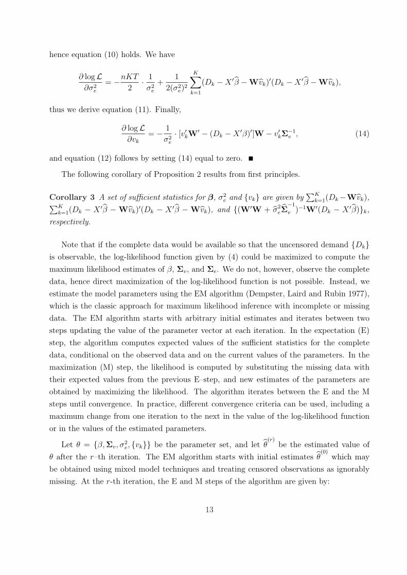
thus we derive equation (11). Finally,
∂ logL∂vk
= − 1
σ2e
· [v′kW′ − (Dk −X ′β)′]W − v′kΣ−1v , (14)
and equation (12) follows by setting (14) equal to zero.
The following corollary of Proposition 2 results from first principles.
Corollary 3 A set of sufficient statistics for β, σ2e and {vk} are given by
∑Kk=1(Dk−Wvk),∑K
k=1(Dk − X ′β − Wvk)′(Dk − X ′β − Wvk), and {(W′W + σ2
eΣ−1
v )−1W′(Dk − X ′β)}k,
respectively.
Note that if the complete data would be available so that the uncensored demand {Dk}is observable, the log-likelihood function given by (4) could be maximized to compute the
maximum likelihood estimates of β, Σv, and Σe. We do not, however, observe the complete
data, hence direct maximization of the log-likelihood function is not possible. Instead, we
estimate the model parameters using the EM algorithm (Dempster, Laird and Rubin 1977),
which is the classic approach for maximum likelihood inference with incomplete or missing
data. The EM algorithm starts with arbitrary initial estimates and iterates between two
steps updating the value of the parameter vector at each iteration. In the expectation (E)
step, the algorithm computes expected values of the sufficient statistics for the complete
data, conditional on the observed data and on the current values of the parameters. In the
maximization (M) step, the likelihood is computed by substituting the missing data with
their expected values from the previous E–step, and new estimates of the parameters are
obtained by maximizing the likelihood. The algorithm iterates between the E and the M
steps until convergence. In practice, different convergence criteria can be used, including a
maximum change from one iteration to the next in the value of the log-likelihood function
or in the values of the estimated parameters.
Let θ = {β,Σv, σ2e, {vk}} be the parameter set, and let θ
(r)be the estimated value of
θ after the r–th iteration. The EM algorithm starts with initial estimates θ(0)
which may
be obtained using mixed model techniques and treating censored observations as ignorably
missing. At the r-th iteration, the E and M steps of the algorithm are given by:
13
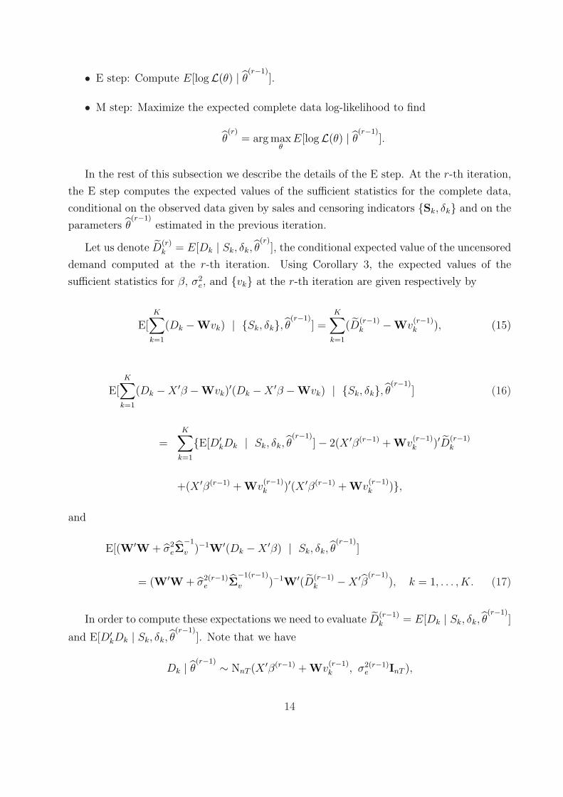
• E step: Compute E[logL(θ) | θ(r−1)].
• M step: Maximize the expected complete data log-likelihood to find
θ(r)
= arg maxθ
E[logL(θ) | θ(r−1)].
In the rest of this subsection we describe the details of the E step. At the r-th iteration,
the E step computes the expected values of the sufficient statistics for the complete data,
conditional on the observed data given by sales and censoring indicators {Sk, δk} and on the
parameters θ(r−1)
estimated in the previous iteration.
Let us denote D(r)k = E[Dk | Sk, δk, θ
(r)], the conditional expected value of the uncensored
demand computed at the r-th iteration. Using Corollary 3, the expected values of the
sufficient statistics for β, σ2e, and {vk} at the r-th iteration are given respectively by
E[K∑
k=1
(Dk −Wvk) | {Sk, δk}, θ(r−1)
] =K∑
k=1
(D(r−1)k −Wv
(r−1)k ), (15)
E[K∑
k=1
(Dk −X ′β −Wvk)′(Dk −X ′β −Wvk) | {Sk, δk}, θ
(r−1)] (16)
=K∑
k=1
{E[D′kDk | Sk, δk, θ
(r−1)]− 2(X ′β(r−1) + Wv
(r−1)k )′D(r−1)
k
+(X ′β(r−1) + Wv(r−1)k )′(X ′β(r−1) + Wv
(r−1)k )},
and
E[(W′W + σ2eΣ
−1
v )−1W′(Dk −X ′β) | Sk, δk, θ(r−1)
]
= (W′W + σ2(r−1)e Σ
−1(r−1)
v )−1W′(D(r−1)k −X ′β
(r−1)), k = 1, . . . , K. (17)
In order to compute these expectations we need to evaluate D(r−1)k = E[Dk | Sk, δk, θ
(r−1)]
and E[D′kDk | Sk, δk, θ
(r−1)]. Note that we have
Dk | θ(r−1) ∼ NnT (X ′β(r−1) + Wv
(r−1)k , σ2(r−1)
e InT ),
14
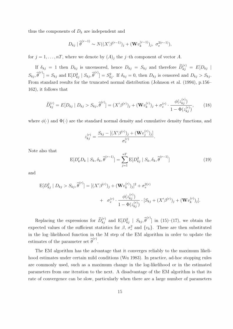
thus the components of Dk are independent and
Dkj | θ(r−1) ∼ N((X ′β(r−1))j + (Wv
(r−1)k )j, σ2(r−1)
e ),
for j = 1, . . . , nT , where we denote by (A)j the j–th component of vector A.
If δkj = 1 then Dkj is uncensored, hence Dkj = Skj and therefore D(r)kj = E[Dkj |
Skj, θ(r)
] = Skj and E[D2kj | Skj, θ
(r)] = S2
kj. If δkj = 0, then Dkj is censored and Dkj > Skj.
From standard results for the truncated normal distribution (Johnson et al. (1994), p.156–
162), it follows that
D(r)kj = E[Dkj | Dkj > Skj, θ
(r)] = (X ′β(r))j + (Wv
(r)k )j + σ(r)
e · φ(z(r)kj )
1− Φ(z(r)kj )
, (18)
where φ(·) and Φ(·) are the standard normal density and cumulative density functions, and
z(r)kj =
Skj − [(X ′β(r))j + (Wv(r)j )j]
σ(r)e
.
Note also that
E[D′kDk | Sk, δk, θ
(r−1)] =
nT∑j=1
E[D2kj | Sk, δk, θ
(r−1)] (19)
and
E[D2kj | Dkj > Skj, θ
(r)] = [(X ′β(r))j + (Wv
(r)k )j]
2 + σ2(r)e
+ σ(r)e · φ(z
(r)kj )
1− Φ(z(r)kj )
· [Skj + (X ′β(r))j + (Wv(r)k )j].
Replacing the expressions for D(r)kj and E[D2
kj | Skj, θ(r)
] in (15)–(17), we obtain the
expected values of the sufficient statistics for β, σ2e and {vk}. These are then substituted
in the log–likelihood function in the M step of the EM algorithm in order to update the
estimates of the parameter set θ(r)
.
The EM algorithm has the advantage that it converges reliably to the maximum likeli-
hood estimates under certain mild conditions (Wu 1983). In practice, ad-hoc stopping rules
are commonly used, such as a maximum change in the log-likelihood or in the estimated
parameters from one iteration to the next. A disadvantage of the EM algorithm is that its
rate of convergence can be slow, particularly when there are a large number of parameters
15

or when a high percentage of the sample data is censored. In the next section, we inves-
tigate the convergence speed of the algorithm under different censoring conditions using a
simulation study.
After convergence of the EM algorithm to the maximum likelihood estimates, the stan-
dard errors of the estimates may be computed using a bootstrap approach (Efron and Tibshi-
rani, 1998, Chapter 6). We illustrate the use of the bootstrap in the applications described
in Section 4.
3 Simulation Experiments
In this section we investigate the performance of the EM algorithm described in Section 2.2
through a series of simulation experiments. The objective of the simulation study is to
examine the effects of demand correlation, degree of censoring and length of selling horizon on
the properties of parameter estimates and on the speed of convergence of the EM algorithm.
We consider the case when the seller offers n = 2 products, with inventory of 40 units
for the first product and 160 units for the second. For example, for airline bookings the
products may correspond to two fare classes (business and economy) on the same itinerary.
The total flight capacity is fixed at 200 seats, with 40 seats allocated to the first fare class
and 160 seats allocated to the second.
We simulated demand for the two products over a time horizon with T = 6, 12, and
20 selling periods. The mean demand βt = (βt,1, βt,2) is uniform across all periods for each
product. The latent shock variances σ2v1 and σ2
v2 are chosen such that the coefficient of
variation of demand is 0.4, and the correlation between demand for the two products takes
values of ρ = 0, 0.3, and 0.6. These choices are typical values in airline demand modelling
(McGill 1995; McGill and van Ryzin 1999). We also choose Wt to be the 2 × 2 identity
matrix for each t = 1, . . . , T , and the error variances to be both equal to σ2e = 1.
The simulation comprised 1000 iterations. At each iteration, we generated K = 500
realizations of demand from model (3) with parameters specified above. The demand vectors
were then censored in order to obtain the sales data, and the percentage of censoring took
the values of 0%, 20% and 40%. The censoring indicators for each demand realization were
also recorded at this stage. We then used the EM algorithm to estimate the parameters of
the demand distribution from the sales data and from the censoring indicators. We assumed
that the algorithm has converged when the maximum relative change in one iteration for all
16

estimates was less than 0.001. Tables 1 and 2 summarize the results of the simulations and
report respectively the empirical bias and the mean squared error of the parameter estimates.
The bias for the estimated parameters is mostly negative, except for the estimate of the
correlation ρ. This shows that the EM algorithm slightly underestimates the true parameter
values. The bias and the mean squared error for all parameters are generally decreasing
with the percentage of censoring. This simply reflects the fact that more information in the
sample naturally leads to better estimates. As expected, the bias and mean squared error
for the estimates of the mean demand in each period β1 and β2 are not affected by either the
length T of the selling horizon, or by the correlation ρ between the components of the latent
random effect v. For estimates of the error variance σ2e and of the random effect variances
σ2v1 and σ2
v2, the bias and the mean squared error decrease with the length of the selling
horizon. For the estimate of the random effect correlation ρ, the bias and the mean squared
error also decrease with T , but they increase with the true value of ρ. The positive impact
of the length T of the selling horizon on the properties of the estimates is to be expected,
since a longer horizon gives more information on the distribution of the latent v, and thus
the estimates should be better.
The results of the simulation study suggest that the estimation approach outlined here
works well in large samples and with relatively long time horizons. This is often the case in
practice; for example, airlines commonly use booking horizons with up to T = 24 snapshots,
and have available sales data for hundreds of previous flights for the purpose of demand
forecasting.
Problems may sometimes arise in the implementation of the EM algorithm. Our simu-
lation experience has shown that in some instances there are singularities in Σv at a given
iteration. In this situation, one could use the estimated value of Σv from the previous it-
eration. For the simulation study reported in this section, we encountered non-convergence
problems in less than 2% of the iterations. Although the EM algorithm has notoriously slow
convergence, it did however converge quite fast in all the simulation scenarios that we con-
sidered, for those iterations where convergence has been achieved. The actual convergence
speed decreased both with increasing percentage of censorship and with increasing demand
correlation.
17
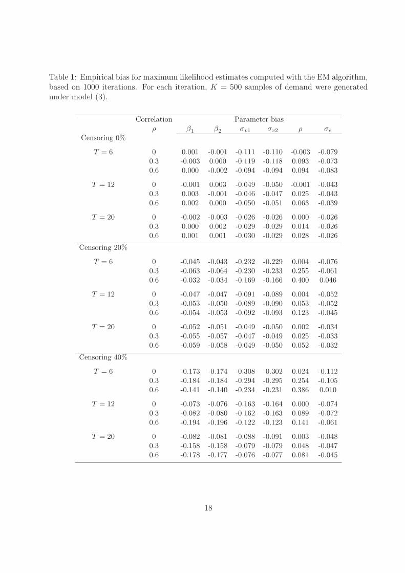
Table 1: Empirical bias for maximum likelihood estimates computed with the EM algorithm,based on 1000 iterations. For each iteration, K = 500 samples of demand were generatedunder model (3).
Correlation Parameter biasρ β1 β2 σv1 σv2 ρ σe
Censoring 0%
T = 6 0 0.001 -0.001 -0.111 -0.110 -0.003 -0.0790.3 -0.003 0.000 -0.119 -0.118 0.093 -0.0730.6 0.000 -0.002 -0.094 -0.094 0.094 -0.083
T = 12 0 -0.001 0.003 -0.049 -0.050 -0.001 -0.0430.3 0.003 -0.001 -0.046 -0.047 0.025 -0.0430.6 0.002 0.000 -0.050 -0.051 0.063 -0.039
T = 20 0 -0.002 -0.003 -0.026 -0.026 0.000 -0.0260.3 0.000 0.002 -0.029 -0.029 0.014 -0.0260.6 0.001 0.001 -0.030 -0.029 0.028 -0.026
Censoring 20%
T = 6 0 -0.045 -0.043 -0.232 -0.229 0.004 -0.0760.3 -0.063 -0.064 -0.230 -0.233 0.255 -0.0610.6 -0.032 -0.034 -0.169 -0.166 0.400 0.046
T = 12 0 -0.047 -0.047 -0.091 -0.089 0.004 -0.0520.3 -0.053 -0.050 -0.089 -0.090 0.053 -0.0520.6 -0.054 -0.053 -0.092 -0.093 0.123 -0.045
T = 20 0 -0.052 -0.051 -0.049 -0.050 0.002 -0.0340.3 -0.055 -0.057 -0.047 -0.049 0.025 -0.0330.6 -0.059 -0.058 -0.049 -0.050 0.052 -0.032
Censoring 40%
T = 6 0 -0.173 -0.174 -0.308 -0.302 0.024 -0.1120.3 -0.184 -0.184 -0.294 -0.295 0.254 -0.1050.6 -0.141 -0.140 -0.234 -0.231 0.386 0.010
T = 12 0 -0.073 -0.076 -0.163 -0.164 0.000 -0.0740.3 -0.082 -0.080 -0.162 -0.163 0.089 -0.0720.6 -0.194 -0.196 -0.122 -0.123 0.141 -0.061
T = 20 0 -0.082 -0.081 -0.088 -0.091 0.003 -0.0480.3 -0.158 -0.158 -0.079 -0.079 0.048 -0.0470.6 -0.178 -0.177 -0.076 -0.077 0.081 -0.045
18
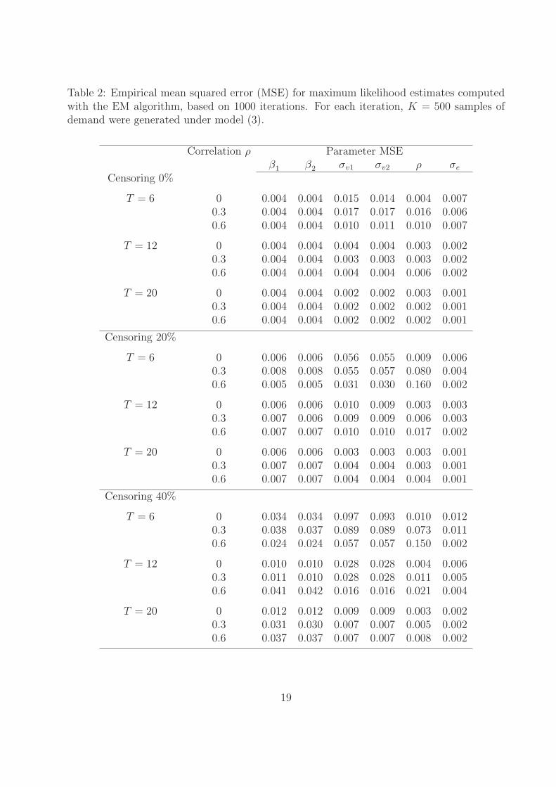
Table 2: Empirical mean squared error (MSE) for maximum likelihood estimates computedwith the EM algorithm, based on 1000 iterations. For each iteration, K = 500 samples ofdemand were generated under model (3).
Correlation ρ Parameter MSEβ1 β2 σv1 σv2 ρ σe
Censoring 0%
T = 6 0 0.004 0.004 0.015 0.014 0.004 0.0070.3 0.004 0.004 0.017 0.017 0.016 0.0060.6 0.004 0.004 0.010 0.011 0.010 0.007
T = 12 0 0.004 0.004 0.004 0.004 0.003 0.0020.3 0.004 0.004 0.003 0.003 0.003 0.0020.6 0.004 0.004 0.004 0.004 0.006 0.002
T = 20 0 0.004 0.004 0.002 0.002 0.003 0.0010.3 0.004 0.004 0.002 0.002 0.002 0.0010.6 0.004 0.004 0.002 0.002 0.002 0.001
Censoring 20%
T = 6 0 0.006 0.006 0.056 0.055 0.009 0.0060.3 0.008 0.008 0.055 0.057 0.080 0.0040.6 0.005 0.005 0.031 0.030 0.160 0.002
T = 12 0 0.006 0.006 0.010 0.009 0.003 0.0030.3 0.007 0.006 0.009 0.009 0.006 0.0030.6 0.007 0.007 0.010 0.010 0.017 0.002
T = 20 0 0.006 0.006 0.003 0.003 0.003 0.0010.3 0.007 0.007 0.004 0.004 0.003 0.0010.6 0.007 0.007 0.004 0.004 0.004 0.001
Censoring 40%
T = 6 0 0.034 0.034 0.097 0.093 0.010 0.0120.3 0.038 0.037 0.089 0.089 0.073 0.0110.6 0.024 0.024 0.057 0.057 0.150 0.002
T = 12 0 0.010 0.010 0.028 0.028 0.004 0.0060.3 0.011 0.010 0.028 0.028 0.011 0.0050.6 0.041 0.042 0.016 0.016 0.021 0.004
T = 20 0 0.012 0.012 0.009 0.009 0.003 0.0020.3 0.031 0.030 0.007 0.007 0.005 0.0020.6 0.037 0.037 0.007 0.007 0.008 0.002
19
4 Applications
In this section we illustrate the modeling methodology developed in Section 2 with the
analysis of two booking data sets from the entertainment and the airline industries.
4.1 Theater Booking Data
Our first illustration uses booking data from a major entertainment venue in London. The
data set records tickets sold during the 2004–2005 season. There are 21 productions staged
on 139 performance dates (hence K = 139), with the number of performances for each pro-
duction varying between three and twelve. We restrict our analysis to evening performances
only, and focus on ticket sales for four parts of the house — the Amphitheater, the Balcony,
the Grand Tier, and the Orchestra Stalls. The tickets are sold in several different price
bands reflecting a decreasing order of prices. In our sample we include sales for four price
bands: PB1 contains tickets for Orchestra Stalls and the Grand Tier, PB2 contains tickets
for Orchestra Stalls only, PB3 contains tickets for the Balcony, and PB4 contains tickets for
the Balcony and the Amphitheater. We define a product as a ticket in one specific price
band, therefore we have n = 4 products. The corresponding capacity limits in each price
band are 490, 177, 112, and 100 seats, and about 15% of the demand observations were
censored.
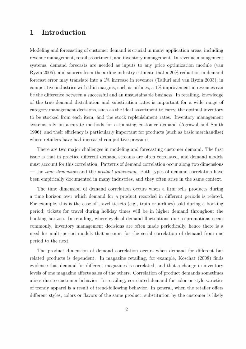
The data set contains a total of 109719 bookings, many of which have been made well
in advance of the performance date. Indeed, the number of advanced purchase days varies
between 0 and 224, with a mean of 88 days, a median of 98 days, and a standard deviation of
54 days. Figure 4.1 gives the histogram of the highly skewed distribution of days of advanced
purchase. An interesting feature of the booking process for theater tickets is that it tends
to be bimodal — a significant proportion of bookings are made three to four months before
the performance, then bookings decline, and finally there is another surge of last-minute
bookings in the week before the performance. For the purpose of our analysis, we aggregate
bookings in seven periods during the horizon, hence T = 7. Period t = 1 is the last week
before the performance, the next period t = 2 is between one month and one week, and the
remaining five periods contain each one month of bookings. This ensures that each period
contains between 10%-20% of the total bookings.
Since tickets in all price bands are normally sold during the entire horizon, we take the
weighting matrices as the 4 × 4 identity matrix, Wt = I4 for t = 1, . . . , 7. No product
attributes were available, so the covariate vector Xt contains only an intercept and the
20
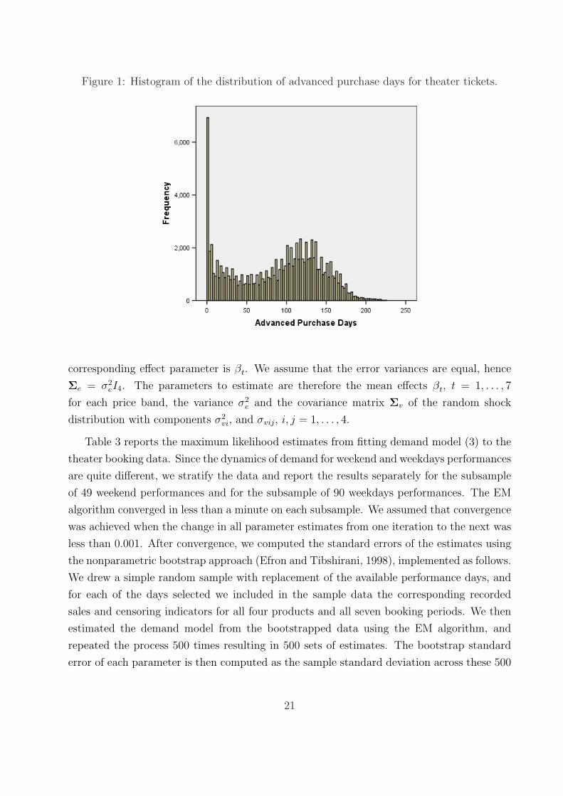
Figure 1: Histogram of the distribution of advanced purchase days for theater tickets.
corresponding effect parameter is βt. We assume that the error variances are equal, hence
Σe = σ2eI4. The parameters to estimate are therefore the mean effects βt, t = 1, . . . , 7
for each price band, the variance σ2e and the covariance matrix Σv of the random shock
distribution with components σ2vi, and σvij, i, j = 1, . . . , 4.
Table 3 reports the maximum likelihood estimates from fitting demand model (3) to the
theater booking data. Since the dynamics of demand for weekend and weekdays performances
are quite different, we stratify the data and report the results separately for the subsample
of 49 weekend performances and for the subsample of 90 weekdays performances. The EM
algorithm converged in less than a minute on each subsample. We assumed that convergence
was achieved when the change in all parameter estimates from one iteration to the next was
less than 0.001. After convergence, we computed the standard errors of the estimates using
the nonparametric bootstrap approach (Efron and Tibshirani, 1998), implemented as follows.
We drew a simple random sample with replacement of the available performance days, and
for each of the days selected we included in the sample data the corresponding recorded
sales and censoring indicators for all four products and all seven booking periods. We then
estimated the demand model from the bootstrapped data using the EM algorithm, and
repeated the process 500 times resulting in 500 sets of estimates. The bootstrap standard
error of each parameter is then computed as the sample standard deviation across these 500
21
sets of estimates. These standard errors are reported in parentheses in Table 3.
The estimated means βt reflect the average bookings for each product in each period.
For tickets in price band PB1 (the most expensive), βt generally increases with t as most of
the bookings tend to be made well in advance of the performance date. This is true for both
weekend and weekdays performances, although for weekdays performances the sequence of
βt has a U-shape pattern; a lot of bookings are made more than four months in advance,
then they decrease, and finally they slightly increase again in the weeks before the perfor-
mance. This is consistent with expectations of customer behaviour; expensive tickets for
weekend performances are mostly purchased four to six months in advance. For weekdays
performances where it may be more difficult to commit so long in advance, most bookings
are clustered either four to six months earlier or in the last few weeks before the performance.
The opposite pattern holds for the less expensive products in price bands PB3 and PB4.
Here relatively few bookings are made in earlier periods t = 6, 7, and a larger proportion
of tickets are purchased in the month before the performance. Note that the values of β1
for tickets in price bands PB3 and PB4 are very similar between weekend and weekdays
performances (11.22 versus 10.98, and 30.23 versus 30.66, respectively), showing that last-
minute demand for cheaper tickets does not depend on whether the performance is on a
weekend or not.
The estimated variances of the latent shock are all statistically significant, showing that
there is significant intertemporal demand dependence for both weekend and weekdays per-
formances. The estimated covariance values are also statistically significant, and lead to
large correlation coefficients between the components of the latent shock. This implies that
there is substantial inter-product demand dependence. The dependence is higher (up to a
correlation coefficient of 0.68) among demand for tickets in price bands PB1 and PB2, likely
due to substitutable demand for the most expensive products.
4.2 Airline Booking Data
The second example of an application of our modeling methodology uses booking data from
a major airline which operates a hub-and-spoke network. The data records tickets sold for
90 departure days of the same flight on a transatlantic route starting from the airline’s hub.
Only flights departing between Monday and Thursday were included in the sample, since
demand for weekend flights may have different characteristics. A product in this setting is
a fare class, and we focus our analysis on bookings for two fare classes (n = 2), which we
22
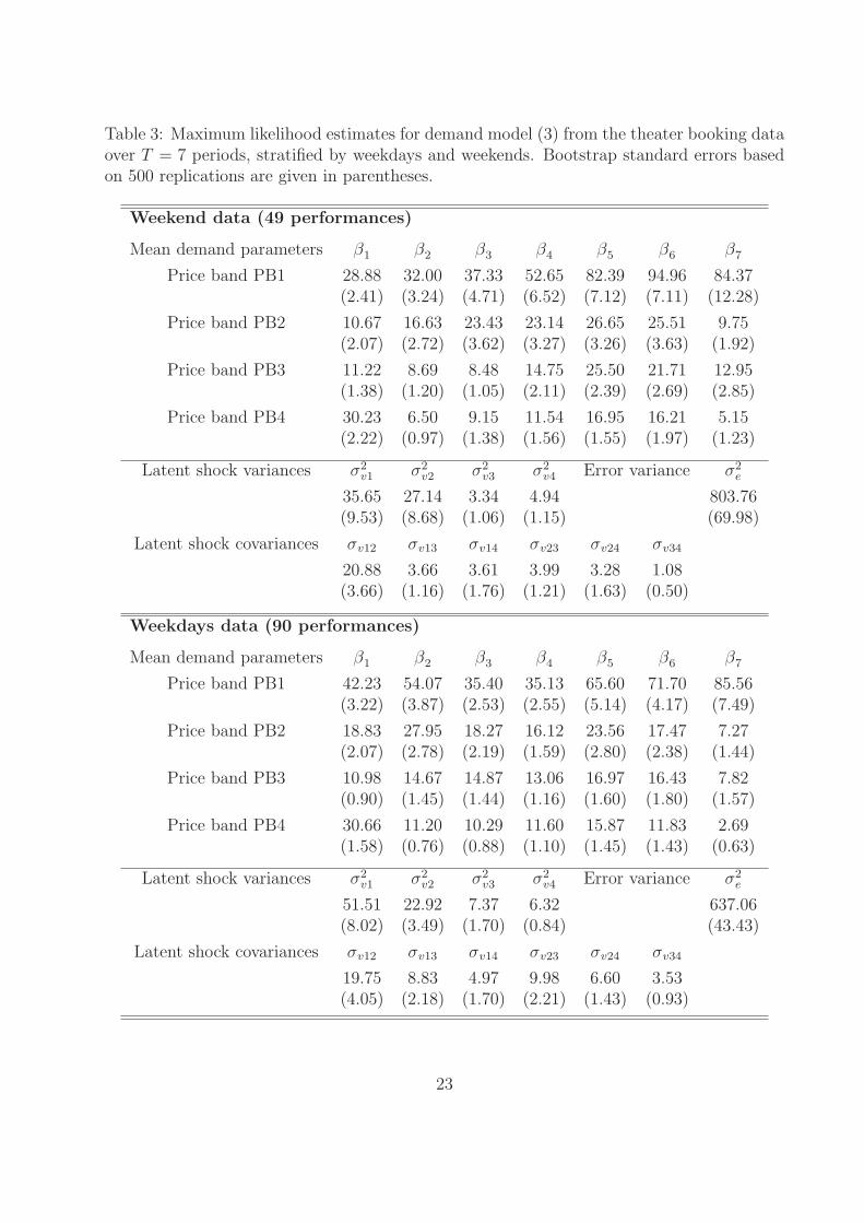
Table 3: Maximum likelihood estimates for demand model (3) from the theater booking dataover T = 7 periods, stratified by weekdays and weekends. Bootstrap standard errors basedon 500 replications are given in parentheses.
Weekend data (49 performances)
Mean demand parameters β1 β2 β3 β4 β5 β6 β7
Price band PB1 28.88 32.00 37.33 52.65 82.39 94.96 84.37(2.41) (3.24) (4.71) (6.52) (7.12) (7.11) (12.28)
Price band PB2 10.67 16.63 23.43 23.14 26.65 25.51 9.75(2.07) (2.72) (3.62) (3.27) (3.26) (3.63) (1.92)
Price band PB3 11.22 8.69 8.48 14.75 25.50 21.71 12.95(1.38) (1.20) (1.05) (2.11) (2.39) (2.69) (2.85)
Price band PB4 30.23 6.50 9.15 11.54 16.95 16.21 5.15(2.22) (0.97) (1.38) (1.56) (1.55) (1.97) (1.23)
Latent shock variances σ2v1 σ2
v2 σ2v3 σ2
v4 Error variance σ2e
35.65 27.14 3.34 4.94 803.76(9.53) (8.68) (1.06) (1.15) (69.98)
Latent shock covariances σv12 σv13 σv14 σv23 σv24 σv34
20.88 3.66 3.61 3.99 3.28 1.08(3.66) (1.16) (1.76) (1.21) (1.63) (0.50)
Weekdays data (90 performances)
Mean demand parameters β1 β2 β3 β4 β5 β6 β7
Price band PB1 42.23 54.07 35.40 35.13 65.60 71.70 85.56(3.22) (3.87) (2.53) (2.55) (5.14) (4.17) (7.49)
Price band PB2 18.83 27.95 18.27 16.12 23.56 17.47 7.27(2.07) (2.78) (2.19) (1.59) (2.80) (2.38) (1.44)
Price band PB3 10.98 14.67 14.87 13.06 16.97 16.43 7.82(0.90) (1.45) (1.44) (1.16) (1.60) (1.80) (1.57)
Price band PB4 30.66 11.20 10.29 11.60 15.87 11.83 2.69(1.58) (0.76) (0.88) (1.10) (1.45) (1.43) (0.63)
Latent shock variances σ2v1 σ2
v2 σ2v3 σ2
v4 Error variance σ2e
51.51 22.92 7.37 6.32 637.06(8.02) (3.49) (1.70) (0.84) (43.43)
Latent shock covariances σv12 σv13 σv14 σv23 σv24 σv34
19.75 8.83 4.97 9.98 6.60 3.53(4.05) (2.18) (1.70) (2.21) (1.43) (0.93)
23
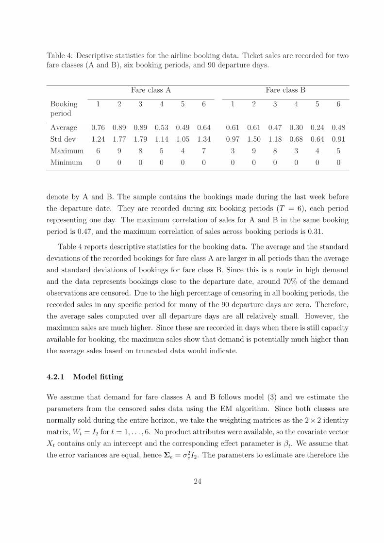
Table 4: Descriptive statistics for the airline booking data. Ticket sales are recorded for twofare classes (A and B), six booking periods, and 90 departure days.
Fare class A Fare class B
Booking 1 2 3 4 5 6 1 2 3 4 5 6period
Average 0.76 0.89 0.89 0.53 0.49 0.64 0.61 0.61 0.47 0.30 0.24 0.48
Std dev 1.24 1.77 1.79 1.14 1.05 1.34 0.97 1.50 1.18 0.68 0.64 0.91
Maximum 6 9 8 5 4 7 3 9 8 3 4 5
Minimum 0 0 0 0 0 0 0 0 0 0 0 0
denote by A and B. The sample contains the bookings made during the last week before
the departure date. They are recorded during six booking periods (T = 6), each period
representing one day. The maximum correlation of sales for A and B in the same booking
period is 0.47, and the maximum correlation of sales across booking periods is 0.31.
Table 4 reports descriptive statistics for the booking data. The average and the standard
deviations of the recorded bookings for fare class A are larger in all periods than the average
and standard deviations of bookings for fare class B. Since this is a route in high demand
and the data represents bookings close to the departure date, around 70% of the demand
observations are censored. Due to the high percentage of censoring in all booking periods, the
recorded sales in any specific period for many of the 90 departure days are zero. Therefore,
the average sales computed over all departure days are all relatively small. However, the
maximum sales are much higher. Since these are recorded in days when there is still capacity
available for booking, the maximum sales show that demand is potentially much higher than
the average sales based on truncated data would indicate.
4.2.1 Model fitting
We assume that demand for fare classes A and B follows model (3) and we estimate the
parameters from the censored sales data using the EM algorithm. Since both classes are
normally sold during the entire horizon, we take the weighting matrices as the 2× 2 identity
matrix, Wt = I2 for t = 1, . . . , 6. No product attributes were available, so the covariate vector
Xt contains only an intercept and the corresponding effect parameter is βt. We assume that
the error variances are equal, hence Σe = σ2eI2. The parameters to estimate are therefore the
24
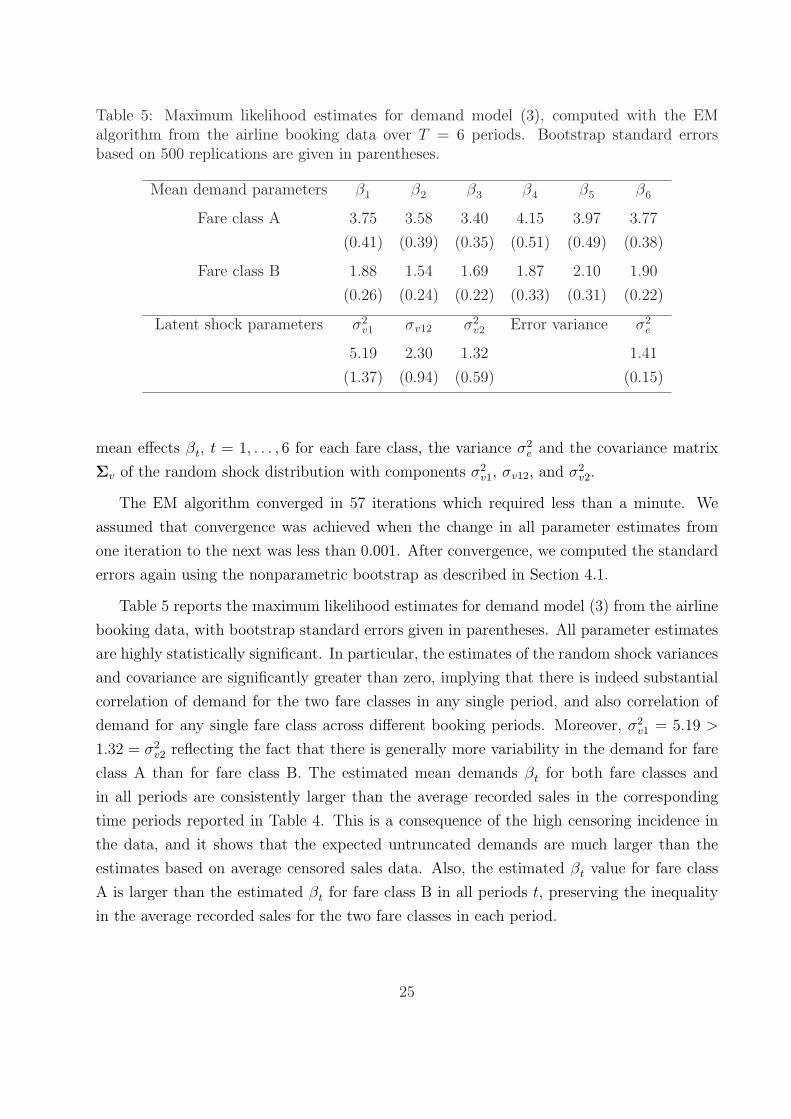
Table 5: Maximum likelihood estimates for demand model (3), computed with the EMalgorithm from the airline booking data over T = 6 periods. Bootstrap standard errorsbased on 500 replications are given in parentheses.
Mean demand parameters β1 β2 β3 β4 β5 β6
Fare class A 3.75 3.58 3.40 4.15 3.97 3.77
(0.41) (0.39) (0.35) (0.51) (0.49) (0.38)
Fare class B 1.88 1.54 1.69 1.87 2.10 1.90
(0.26) (0.24) (0.22) (0.33) (0.31) (0.22)
Latent shock parameters σ2v1 σv12 σ2
v2 Error variance σ2e
5.19 2.30 1.32 1.41
(1.37) (0.94) (0.59) (0.15)
mean effects βt, t = 1, . . . , 6 for each fare class, the variance σ2e and the covariance matrix
Σv of the random shock distribution with components σ2v1, σv12, and σ2
v2.
The EM algorithm converged in 57 iterations which required less than a minute. We
assumed that convergence was achieved when the change in all parameter estimates from
one iteration to the next was less than 0.001. After convergence, we computed the standard
errors again using the nonparametric bootstrap as described in Section 4.1.
Table 5 reports the maximum likelihood estimates for demand model (3) from the airline
booking data, with bootstrap standard errors given in parentheses. All parameter estimates
are highly statistically significant. In particular, the estimates of the random shock variances
and covariance are significantly greater than zero, implying that there is indeed substantial
correlation of demand for the two fare classes in any single period, and also correlation of
demand for any single fare class across different booking periods. Moreover, σ2v1 = 5.19 >
1.32 = σ2v2 reflecting the fact that there is generally more variability in the demand for fare
class A than for fare class B. The estimated mean demands βt for both fare classes and
in all periods are consistently larger than the average recorded sales in the corresponding
time periods reported in Table 4. This is a consequence of the high censoring incidence in
the data, and it shows that the expected untruncated demands are much larger than the
estimates based on average censored sales data. Also, the estimated βt value for fare class
A is larger than the estimated βt for fare class B in all periods t, preserving the inequality
in the average recorded sales for the two fare classes in each period.
25
4.2.2 Demand untruncation
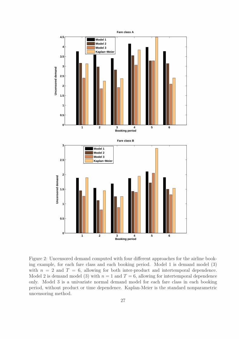
In this subsection we compare the predictions of untruncated demand computed with the
multivariate multiperiod demand model (3) for the airline data to the predictions computed
with three alternative approaches. The goal of this comparison is to assess the impact that
accounting for demand dependence has on the untruncated demand predictions.
We consider the following models: Model 1 is the most general form of expression (3) with
n = 2 and T = 6, accounting for both inter-product and intertemporal dependence. Model 2
is a restricted form of expression (3) with n = 1 and T = 6, allowing for intertemporal
dependence but not inter-product dependence. Model 3 is an univariate normal demand
model for each fare class in each booking period, and it does not capture either inter-
product or intertemporal dependence. Finally, we consider the predictions from the standard
nonparametric uncensoring method developed by Kaplan and Meier (1958).
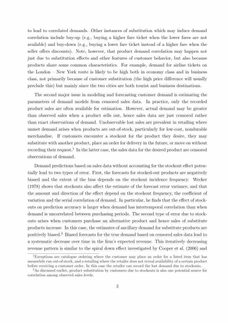
Figure 2 gives the uncensored demand predicted with each of the four methods, for both
fare classes and all six booking periods. The values predicted by Model 1 which accounts
for both inter-product and inter-temporal correlation are larger than those predicted by
Models 2 and 3 which ignore some or all dependence patterns. Predictions from Model 1 are
also generally larger than the uncensored values computed with the nonparametric Kaplan-
Meier method, except for booking period t = 5.
4.2.3 Protection levels with dependent demand
In this subsection we show how, in a revenue management setting, the multivariate multi-
period demand model (3) can influence the computation of protection levels for different fare
products. We then assess the resulting impact on revenue through a small simulation study
that mimics the booking patterns found in the airline booking data in Section 4.2.1.
We focus on a simple and effective heuristic for computing protection levels developed by
Belobaba (1987) for the single-leg problem. This heuristic based on the expected marginal
seat revenue (EMSR-b) is widely used in practice. It considers fare classes 1 through n
sorted in decreasing order of their revenues p1 > . . . > pn−1 > pn, and it computes the
nested protection levels b = (b1, . . . , bn−1), where bi is the capacity to be reserved for all
fare classes 1, . . . , i. A request for fare class i + 1 is then fulfilled only if the remaining
capacity is greater than bi. Brumelle and McGill (1993) showed that this policy is optimal
when demands are independent and when demand for low-fare products arrives earlier then
demand for high-fare products.
26
1 2 3 4 5 60
0.5
1
1.5
2
2.5
3
3.5
4
4.5
Booking period
Unc
enso
red
dem
and
Fare class A
Model 1Model 2Model 3Kaplan−Meier
1 2 3 4 5 60
0.5
1
1.5
2
2.5
3
Booking period
Unc
enso
red
dem
and
Fare class B
Model 1Model 2Model 3Kaplan−Meier
Figure 2: Uncensored demand computed with four different approaches for the airline book-ing example, for each fare class and each booking period. Model 1 is demand model (3)with n = 2 and T = 6, allowing for both inter-product and intertemporal dependence.Model 2 is demand model (3) with n = 1 and T = 6, allowing for intertemporal dependenceonly. Model 3 is a univariate normal demand model for each fare class in each bookingperiod, without product or time dependence. Kaplan-Meier is the standard nonparametricuncensoring method.
27
Specifically, let µi and σ2i be the mean and variance of demand for fare class i, for all
i ∈ {1, . . . , n}. Let p∗i =∑i
j=1 piµi/∑i
j=1 µi be the weighted average revenue from the first
i fare classes. The booking limit bi is defined as the quantile of the normal distribution
that satisfies pi+1 = p∗i Pr(X∗i > bi), where X∗
i ∼ N(∑i
j=1 µi,∑i
j=1 σ2i ) is a normal random
variable that intuitively represents the cumulative demand for the first i fare classes.
We focus our comparison on two demand models which we use in order to estimate
the means and variances µi and σ2i of demand for each fare class. The benchmark is a
simple univariate normal demand model for each fare class in each booking period, that
does not capture either inter-product or intertemporal demand dependence. The second
demand model is the multivariate formulation (3) accounting for both product and serial
correlation of demand. Under this model, the estimated means and variances µi and σ2i in
period t are computed conditional on demand for both products observed up to time t, using
the well-known general formulas for conditional means and variances of multivariate normal
distributions.6 Intuitively, the conditional means and variances contain information about
past demand and, as demand unfolds over the booking horizon, they convey more information
for the computation of protection levels than the estimates based on the univariate demand
model that ignores past demand information.
We ran a small simulation study in order to identify the impact on revenue from using
the multivariate demand model in the computation of protection levels. We endeavored to
mimic the demand patterns from the airline booking data that we analyzed in the previous
subsections. For the simulation design we thus chose a setting with two products (n = 2)
and six booking periods (T = 6). We assumed that random product demand exhibits both
inter-product and intertemporal dependence, however in order to check the robustness of our
methodology we did not assume that demand was generated from model (3). Instead, we
generated demand from the multivariate normal distribution NnT (β, WΣvW′ + σ2
e × InT ),
where W is the nT × n matrix obtained by stacking T times the identity matrix In, and
Σv, σ2e and β have components given by the estimated values from Table 5. This choice of
parameters ensures that random product demand is similar to that recorded in the airline
6For any random vectors X1 and X2 with a multivariate normal distribution such that(
X1
X2
)∼ N
((ν1
ν2
),
(Σ11 Σ12
Σ21 Σ22
)),
we haveE[X1 | X2 = x] = ν1 + Σ12Σ−1
22 (x− ν2),
andV ar[X1 | X2 = x] = Σ11 − Σ12Σ−1
22 Σ21.
28
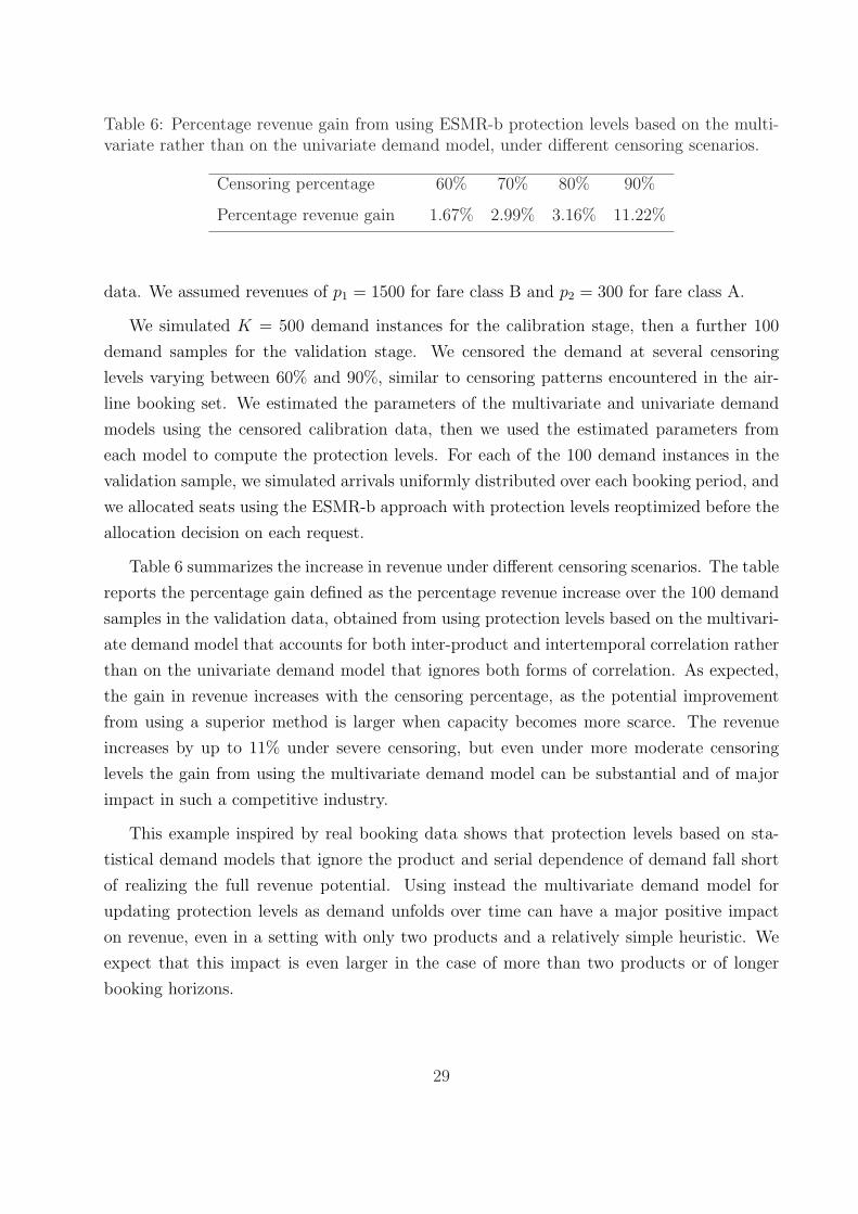
Table 6: Percentage revenue gain from using ESMR-b protection levels based on the multi-variate rather than on the univariate demand model, under different censoring scenarios.
Censoring percentage 60% 70% 80% 90%
Percentage revenue gain 1.67% 2.99% 3.16% 11.22%
data. We assumed revenues of p1 = 1500 for fare class B and p2 = 300 for fare class A.
We simulated K = 500 demand instances for the calibration stage, then a further 100
demand samples for the validation stage. We censored the demand at several censoring
levels varying between 60% and 90%, similar to censoring patterns encountered in the air-
line booking set. We estimated the parameters of the multivariate and univariate demand
models using the censored calibration data, then we used the estimated parameters from
each model to compute the protection levels. For each of the 100 demand instances in the
validation sample, we simulated arrivals uniformly distributed over each booking period, and
we allocated seats using the ESMR-b approach with protection levels reoptimized before the
allocation decision on each request.
Table 6 summarizes the increase in revenue under different censoring scenarios. The table
reports the percentage gain defined as the percentage revenue increase over the 100 demand
samples in the validation data, obtained from using protection levels based on the multivari-
ate demand model that accounts for both inter-product and intertemporal correlation rather
than on the univariate demand model that ignores both forms of correlation. As expected,
the gain in revenue increases with the censoring percentage, as the potential improvement
from using a superior method is larger when capacity becomes more scarce. The revenue
increases by up to 11% under severe censoring, but even under more moderate censoring
levels the gain from using the multivariate demand model can be substantial and of major
impact in such a competitive industry.
This example inspired by real booking data shows that protection levels based on sta-
tistical demand models that ignore the product and serial dependence of demand fall short
of realizing the full revenue potential. Using instead the multivariate demand model for
updating protection levels as demand unfolds over time can have a major positive impact
on revenue, even in a setting with only two products and a relatively simple heuristic. We
expect that this impact is even larger in the case of more than two products or of longer
booking horizons.
29
5 Conclusions
Much research effort has been devoted to building models and developing algorithms to
improve operational decisions in diverse fields such as inventory control, supply chain man-
agement and revenue management. What often stands between models and practice is the
population of model parameters. Accurately estimating parameters and fitting models to
data can make a big difference in revenues and an even bigger difference in profits for many
firms. Yet the problem of model calibration from data and of parameter estimation is usu-
ally not addressed in research papers that focus generally on the stochastic or algorithmic
aspects of the models. This paper aims to bridge the gap between the theoretical develop-
ment of models and their implementation in operations applications that require multivariate
demand formulations. We show how improved demand estimates lead to better decisions
and how statistical calibration is key in deploying and increasing the impact of models and
algorithms.
We have investigated in this paper a class of multivariate demand models that can ac-
count for both time dependence and product dependence of demand. These dependence
features occur often in practice in a wide range of applications, most commonly arising from
substitution and cross–selling effects, or from censoring due to capacity constraints. It is
therefore important to capture these demand dependence patterns in order to obtain un-
biased and efficient estimates of future demand. The class of models that we investigate
here have the flexibility to account for a range of dependence patterns through the inclusion
of the common multivariate latent shock. The models could also be extended to include a
stochastic autocorrelated process (for example a mean-reverting process) for the latent vt.
We have also developed in this paper a methodology for estimating the parameters of
multivariate and multi-period demand models from censored sales data. We have shown
through simulation experiments that our approach based on the EM algorithm is computa-
tionally attractive, and that it leads to maximum likelihood estimates with good properties
under a range of demand and censoring scenarios. Although the convergence of the EM al-
gorithm is notoriously slow, in our numerical experience with simulations and with practical
examples the algorithm has converged relatively fast.
We have illustrated our methodology with the analysis of two booking data sets from
the entertainment and the airline industries. We showed that there is strong evidence of
significant intertemporal and interproduct correlation in bookings of theater tickets, and
uncovered the dynamics of the booking process during the sales horizon for tickets in different
price bands. For the airline booking data, we also showed that the uncensored demand
30
predicted by the multivariate models is generally higher than the uncensored values predicted
by other models which ignore some or all patterns of dependence. In addition, we exemplified
the use of the multivariate demand models for computing protection levels in a revenue
management setting, and found that they lead to a substantial increase in revenue relative
to the use of protection levels based on univariate demand models.
Among other applications, the demand models and estimation methodology investigated
in this paper are useful for the development of inventory management methods for retailing.
In a setting with multiple substitutable products, it is important for manufacturers and
retailers to assess how the absence of one product affects the demand for other similar
products. For example, due to space restrictions, the Macy’s department store chain offers
collections with fewer color variants in small stores than in larger stores. It is then critical
to determine the subset of products that will sell best and the optimal inventory levels, and
the models discussed in this paper can help achieve this.
The methodology that we developed here can also be used for revenue management pur-
poses. We outlined in Section 4.2.3 the use of the multivariate demand models for computing
protection levels and showed that this leads to a substantial increase in revenue even with
a simple protection level policy and in a two-product setting. These demand models have
also been used in connection with multistage stochastic programming in order to compute
optimal product prices — DeMiguel and Mishra (2006) give an early example of their ap-
plication in connection with pricing. The practical implementation of the multivariate and
multi-period demand models in other application areas and the implications of their use for
pricing purposes are potential topics of future research.
Acknowledgment
We are grateful to Victor de Miguel, Guillermo Gallego and Bruce Hardie for their comments
and suggestions at various stages of preparation of this manuscript. The support of an RAMD
grant from London Business School is gratefully acknowledged.
References
Agrawal, N., S.A. Smith 1996. Estimating negative binomial demand for retail inventory manage-
ment with unobservable lost sales. Naval Research Logistics 43 839–861.
31
Anupindi, R., M. Dada, S. Gupta 1998. Estimation of consumer demand with stock-out based
substitution: An application to vending machine products. Marketing Science 17 406–423.
Belobaba, P.P. 1987. Air travel demand and airline seat inventory management. Ph.D. thesis,
Massachusetts Institute of Technology, Cambridge, MA.
Brumelle, S.L., J.I. McGill 1993. Airline seat allocation with multiple nested fare classes. Operations
Research 41 127–137.
Cachon, G.P., C. Terwiesch, Y. Xu 2005. Retail assortment planning in the presence of consumer
search. Manufacturing and Service Operations Management 7 330–346.
Conlon, C.T., J.H. Mortimer 2007. Demand estimation under incomplete product availability.
Working paper, Harvard University.
Cooper, W.L., Homem-de-Mello, T., A.J. Kleywegt 2006. Models of the spiral-down effect in revenue
management. Operations Research 54 968–987.
DeMiguel, V., N. Mishra 2006. What multistage stochastic programming can do for network revenue
management. Working paper, London Business School.
Dempster, A.P., N.M. Laird, D.B. Rubin 1977. Maximum likelihood from incomplete data via the
EM algorithm (with discussion). Journal of the Royal Statistical Society, B 39 1–38.
Efron, B., R.J. Tibshirani 1998. An Introduction to the Bootstrap, Chapman and Hall, Boca Raton.
Johnson, N.L., S. Kotz, N. Balakrishnan 1994. Continuous Univariate Distributions. Volume 1, 2nd
Edition, Wiley, New York.
Kaplan, E.L., P. Meier 1958. Nonparametric estimation from incomplete observations. Journal of
the American Statistical Association 53 457–481.
Klein, J.P., M.L. Moeschberger 2005. Survival Analysis, Springer, New York.
Kok, A.G., M.L. Fisher 2007. Demand estimation and assortment optimization under substitution:
Methodology and application. Operations Research 55 1001–1021.
Koschat, M.A 2008. Store inventory can affect demand: Empirical evidence from magazine retailing.
Journal of Retailing 84 165–179.
Lariviere, M., E.L. Porteus 1999. Stalking information: Bayesian inventory management with un-
observed lost sales. Management Science 45 346–358.
Lau, H.S., A.H. Lau 1996. Estimating the demand distributions of single-period items having
frequent stockouts. European Journal of Operational Research 92 254–265.
Lawless, J.F. 2003. Statistical Models and Methods for Lifetime Data, Wiley, New York.
McGill, J.I 1995. Censored regression analysis of multiclass passenger demand data subject to joint
capacity constraints. Annals of Operations Research 60 209–240.
McGill, J.I., G.J. van Ryzin 1999. Revenue management: Research overview and prospects. Trans-
portation Science 33 233–256.
32
Nahmias, S. 1994. Demand estimation in lost sales inventory systems. Naval Research Logistics 41
739–757.
Queenan, C.C., M. Ferguson, J. Higbie, R. Kapoor 2007. A comparison of unconstraining methods
to improve revenue management systems. Production and Operations Management 16 729–
746.
Ratliff, R.M., B.V. Rao, C.P. Narayan, K. Yellepeddi 2008. A multi-flight recapture heuristic for
estimating unconstrained demand from airline bookings. Journal of Revenue and Pricing Man-
agement 7 153–171.
Rossi, P.E., G. Allenby, R. McCulloch 2006. Bayesian Statistics and Marketing. Wiley, New York.
Schneider, H., G.P. Barker 1989. Matrices and Linear Algebra. Dover, New York.
Talluri, K., G.J. van Ryzin 2003. The Theory and Practice of Revenue Management. Kluwer Aca-
demic Press.
Talluri, K., G.J. van Ryzin 2004. Revenue management under a general discrete choice model of
consumer behaviour. Management Science 50 15–33.
Tan, B., S. Karabati 2004. Can the desired service level be achieved when the demand and lost
sales are unobserved? IIE Transactions 36 345–358.
van Ryzin, G. 2005. Future of revenue management: Models of demand. Journal of Revenue and
Pricing Management 4 204–210.
van Ryzin, G., and S. Mahajan 1999. On the relationship between inventory costs and variety
benefits in retail assortments. Management Science 45 1496–1509.
van Ryzin, G., and J. McGill 2000. Revenue management without forecasting or optimization:
An adaptive algorithm for determining airline seat protection levels. Management Science 50
15–33.
Vulcano, G., G. van Ryzin, R. Ratliff 2008. Estimating primary demand for substitutable products
from sales transaction data. Working paper, Columbia Business School.
Weatherford, L.R., and S. Polt 2002. Better unconstraining of airline demand data in revenue
management systems for improved forecast accuracy and greater revenues. Journal of Revenue
and Pricing Management 1 234–254.
Wecker, W.E. 1978. Predicting demand from sales data in the presence of stockouts. Management
Science 24 1043–1054.
Wu, C.F. 1983. On the convergence properties of the EM algorithm. The Annals of Statistics 11
95–103.
33