MultiWell User Manual-2020 - University of Michigan

i

October 1, 2020

MultiWell Program Suite

User Manual

(MultiWell-2020.3)

John R. Barker, T. Lam Nguyen, John F. Stanton, Chiara Aieta, Michele Ceotto, Fabio Gabas, T. J. Dhilip Kumar,

Collin G. L. Li, Lawrence L. Lohr, Andrea Maranzana, Nicholas F. Ortiz, Jack M. Preses, John M. Simmie,

Jason A. Sonk, and Philip J. Stimac

University of Michigan Ann Arbor, MI 48109-2143

Contact: [email protected]

(734) 763-6239

MultiWell Web site: clasp-research.engin.umich.edu/multiwell

(Copyright 2020, John R. Barker)

ii

CONTENTS

0. Preliminaries 1About the Authors 1MultiWell Literature Citations 2Help! Comments! Bug Reports! 3Acknowledgements 3

1. Getting Started 51.1 Software Tools in the MultiWell Suite 51.2 How the Tools Work Together 91.3 Examples and Models 131.4 Installing and Executing the Codes 161.5 Some Technical Issues on Input/Output Files 19References 20

2. MultiWell Master Equation Code 222.1 Brief Description 222.2 Terminology 222.3 Default Array Dimensions 242.4 Notes on FORTRAN source code and compilation 242.5 MultiWell Input Files and Program Execution 252.6 MultiWell Output Files 262.7 MultiWell Input Data File (FileName.dat) 282.8 Collision Models 372.9 Format of External Data Files 412.10 Fatal Input Errors and Warnings 44References 46

3. Separable Molecular Degrees of Freedom 483.1 Types of Degrees of Freedom 483.2 Format for Input Files 53References 57

4. DenSum: Separable Sums and Densities of States 584.1 DenSum Data File Format 584.2 DenSum in Batch Mode 60

iii

References 62

5. MomInert: Moments of Inertia 635.1 Data File Format 635.2 Computational Approach 65References 65

6. thermo: Thermodynamics 666.1 Introduction 666.2 Data File Format 726.3 MultiWell Thermodynamics Database 76References 76

7. gauss2multi: A Tool for Creating Data Files 78References 80

8. bdens, paradensum, parsctst, and sctst: non-Separable Vibrations 82

8.1 Program bdens 838.2 Program paradensum 898.3 Program sctst 948.4 Program parsctst 99References 104

9. lamm: Effective Mass for Internal Rotation 1069.1 Introduction 1069.2 Compiling and Running lamm 1069.3 Notes and Limits 1079.4 Data File Format 1079.5 Example Data File 1089.6 Example Output: 1089.7 gauss2lamm: A script for generating lamm.dat 109References 111

10. ktools: J-Resolved Variational Transition State Theory 11310.1 Introduction 11310.2 Theory 11410.3 ktools Input File 12110.4 Running ktools 12410.5 ktools Output Files 12510.6 ktools Examples 126References 133

11. TS: J-Resolved Steady-State Master Equation Solver 134

iv

Appendix A. Theoretical Basis 135A.1. Introduction 135A.2. The Active Energy Master Equation 135A.3. Stochastic Method 150A.4. Processes 153A.5. Initial Conditions 179A.6. Input 182A.7. Output 183A.8. Concluding Remarks 184References 186

Appendix B. Technical Notes 188B.1 Conversion Factors (Rotational Data) 188B.2 Anharmonic Vibrations 188B.3 Vibrational Degeneracies 192B.4 External molecular rotations 192B.5 Symmetry numbers, internal rotation, and optical isomers (mirror images) 195B.6 A Handy List of Lennard-Jones Parameters 201B.7 Elements and Isotopes in MomInert and Thermo 202B.8 Eigenstates for large amplitude motions 203B.9 Semi-Classical Transition State Theory (SCTST) 207B.10 Legacy and Current Versions of k0 and k∞ in MultiWell 214

Appendix C. How to … 219C.1 How to set up the double arrays in MultiWell 219C.2 How to test the double-array parameters in MultiWell 220C.3 How estimate Lennard-Jones and energy transfer parameters 220C.4 How to obtain rate constants from MultiWell simulations 221C.5 How to tell if the simulated time is long enough 232C.6 How to deal with Barrierless Reactions 235C.7 Some Questions and Answers 236

Index 240

1

0. Preliminaries

About the Authors JOHN BARKER wrote or contributed to most of the codes. The original set of codes was based

on his 1983 paper and subsequent developments.3-7,9 LAM NGUYEN installed a method for using quantum eigenvalues for hindered internal

rotations, wrote a code for computing the effective mass of large amplitude motions, and helped in developing codes for non-separable vibrations,7 and semi-classical transition state theory (SCTST).8 In addition, he and John Stanton are responsible for the code TS.

JOHN STANTON was a key participant in implementing semi-classical transition state theory 8

and vibrational anharmonicities in his quantum chemistry code CFOUR.10 He and Lam Nguyen also are responsible for the code TS.

CHIARA AIETA, FABIO GABAS, and MICHELE CEOTTO (Università degli Studi di Milano)

developed paradensum, a parallelized code1 for computing sums and densities of states for fully coupled vibrational models, and parsctst a parallelized code2 for computing cumulative reaction probabilies from Semi-Classical Transition State Theory (SCTST).

DHILIP KUMAR wrote several scripts for automatically using output files from electronic

structure programs to build input/output files. COLLIN LI wrote much of the code for program bdens. LARRY LOHR contributed to the development of hindered rotor subroutines. ANDREA MARANZANA (University of Turin) contributed codes for automatically generating

input files for the MultiWell Suite from output files produced in quantum chemical calculations.

NICK ORTIZ (as an undergraduate student) wrote most of the code for MOMINERT. JACK PRESES (Brookhaven Nat'l Lab.) added several helpful features. JOHN SIMMIE (Galway, Ireland) is helping to maintain and extend the MultiWell

Thermodynamics Database. JASON SONK wrote most of the code for ktools and has contributed to other codes as well. PHIL STIMAC implemented 1-dimensional quantum tunneling via an unsymmetrical Eckart

barrier in the multiwell master equation code.

2

MultiWell Literature Citations Please cite the following papers to acknowledge results obtained using this version of the

MultiWell Program Suite:

For citing the MultiWell Program Suite In the following, <version> refers to the version number (e.g. 2020.3) and <year> refers to the year of publication (e.g. 2020): (a) J. R. Barker, T. L. Nguyen, J. F. Stanton, C. Aieta, M. Ceotto, F. Gabas, T. J. D. Kumar,

C. G. L. Li, L. L. Lohr, A. Maranzana, N. F. Ortiz, J. M. Preses, J. M. Simmie, J. A. Sonk, and P. J. Stimac; MultiWell-<version> Software Suite; J. R. Barker, University of Michigan, Ann Arbor, Michigan, USA, <year>; http://clasp-research.engin.umich.edu/multiwell/.

(b) John R. Barker, Int. J. Chem. Kinetics, 33, 232-45 (2001). (c) John R. Barker, Int. J. Chem. Kinetics, 41, 748-763 (2009).

References for program bdens References (a) through (c), above, plus … (d) M. Basire, P. Parneix, and F. Calvo, J. Chem. Phys. 129, 081101 (2008). (e) F. Wang and D. P. Landau, Phys. Rev. Letters 86, 2050 (2001). (f) Thanh Lam Nguyen and John R. Barker, J. Phys. Chem. A., 114, 3718–3730 (2010).

References for program paradensum References (a) through (f), above, plus … (g) C. Aieta, F. Gabas, and M. Ceotto, J. Phys. Chem. A, DOI: 10.1021/acs.jpca.5b12364 (2016).

References for program sctst References (a) through (c), above, plus … (h) W. H. Miller, J. Chem. Phys. 62, 1899 (1975). (i) W. H. Miller, Faraday Discuss. Chem. Soc. 62, 40 (1977). (j) W. H. Miller, R. Hernandez, N. C. Handy, D. Jayatilaka, and A. Willets, Chem. Phys. Letters 172, 62 (1990). (k) R. Hernandez and W. H. Miller, Chem. Phys. Lett. 214 (2), 129 (1993). (l) T. L. Nguyen, J. F. Stanton, and J. R. Barker, Chem. Phys. Letters 499, 9 (2010). (m) T. L. Nguyen, J. F. Stanton, and J. R. Barker, J. Phys. Chem. A 115, 5118 (2011).

References for program parsctst References (a) through (c), above, plus References (h) through (m), above, plus (n) Aieta C.; Gabas, F.; Ceotto, M. Parallel Implementation of Semiclassical Transition State Theory J. Chem. Theory Comput. 2019, DOI: 10.1021/acs.jctc.8b01286.

References for program TS Reference (a), above, plus …

3

(o) "TS is a chemical kinetic program that solves a two-dimensional master-equation for gas-phase reactions in parallel using the Steady-State approach. It is developed, implemented, and maintained by T. L. Nguyen and J. F. Stanton, version 01-03-2017."

(p) T. L. Nguyen and J. F. Stanton, A Steady-State Approximation to the Two-Dimensional Master Equation for Chemical Kinetics Calculations, J. Phys. Chem. A 119, 7627-7636 (2015).

(q) T. L. Nguyen, H. Lee, D. A. Matthews, M. C. McCarthy and J. F. Stanton, Stabilization of the Simplest Criegee Intermediate from the Reaction between Ozone and Ethylene: A High-Level Quantum Chemical and Kinetic Analysis of Ozonolysis, J. Phys. Chem. A 119, 5524-5533 (2015).

Help! Comments! Bug Reports! Please send pleas for help, comments, and bug reports to the "Multiwell and Chemical

Kinetics" question and answer forum: all users are invited to join the forum, where questions can be asked and answered, and future upgrades will be announced. This forum is set up as a Google Group, which you can join at https://groups.google.com/. If for any reason it is difficult for you to use Google, please contact John R. Barker ([email protected]) and he will answer your question or pass it along to the appropriate person.

Acknowledgements Thanks go to the following people for particularly helpful suggestions, discussions, de-

bugging, or other assistance: Amity Andersen Keith Kuwata A. Bencsura George Lendvay Hans-Heinrich Carstensen Robert G. ('Glen') MacDonald Gabriel R. Da Silva David M. Matheu Theodore S. Dibble Nigel W. Moriarty David Edwards William F. Schneider Benj FitzPatrick Colleen Shovelin Michael Frenklach Robert M. Shroll David M. Golden Gregory P. Smith Erin Greenwald Al Wagner John Herbon Ralph E. Weston, Jr. Keith D. King Milad Marinami

Some sections of the computer codes were developed as part of research funded by NSF (Atmospheric Chemistry Division), NASA (Upper Atmosphere Research Program), and NASA (Planetary Atmospheres). JMS thanks the Irish Centre for High-End Computing, ICHEC, for the provision of computational resources, ngche041c.

4

Disclaimer: This material is based in part upon work supported by the U.S. National Science Foundation. Any opinions, findings, and conclusions or recommendations expressed in this material are those of the author(s) and do not necessarily reflect the views of the National Science Foundation.

References (1) Aieta, C.; Gabas, F.; Ceotto, M. An Efficient Computational Approach for the

Calculation of the Vibrational Density of States. J. Phys. Chem. A. 2016, DOI: 10.1021/acs.jpca.1025b12364; DOI: 10.1021/acs.jpca.5b12364.

(2) Aieta, C.; Gabas, F.; Ceotto, M. Parallel Implementation of Semiclassical Transition State Theory. J. Chem. Theory Comput. 2019, 15, 2143-2153; DOI: 10.1021/acs.jctc.8b01286.

(3) Barker, J. R. Monte-Carlo Calculations on Unimolecular Reactions, Energy-Transfer, and IR-Multiphoton Decomposition. Chem. Phys. 1983, 77, 301-318.

(4) Barker, J. R. Radiative Recombination in the Electronic Ground State. J. Phys. Chem. 1992, 96, 7361-7367; DOI: 10.1021/j100197a042.

(5) Barker, J. R. Energy Transfer in Master Equation Simulations: A New Approach. Int. J. Chem. Kinet. 2009, 41, 748-763.

(6) Barker, J. R.; King, K. D. Vibrational Energy Transfer in Shock-Heated Norbornene. J. Chem. Phys. 1995, 103, 4953-4966.

(7) Nguyen, T. L.; Barker, J. R. Sums and Densities of Fully-Coupled Anharmonic Vibrational States: A Comparison of Three Practical Methods. J. Phys. Chem. A 2010, 114, 3718–3730.

(8) Nguyen, T. L.; Stanton, J. F.; Barker, J. R. A Practical Implementation of Semi-Classical Transition State Theory for Polyatomics. Chem. Phys. Letters 2010, 499, 9-15.

(9) Shi, J.; Barker, J. R. Incubation in Cyclohexene Decomposition at High Temperatures. Int. J. Chem. Kinet. 1990, 22, 187-206.

(10) Stanton, J. F.; Gauss, J.; Harding, M. E.; Szalay, P. G.; Auer, A. A.; Bartlett, R. J.; Benedikt, U.; Berger, C.; Bernholdt, D. E.; Bomble, Y. J.; Cheng, L.; Christiansen, O.; Heckert, M.; Heun, O.; Huber, C.; Jagau, T.-C.; Jonsson, D.; Jusélius, J.; Klein, K.; Lauderdale, W. J.; Lipparini, F.; Matthews, D. A.; T. Metzroth; Mück, L. A.; O'Neill, D. P.; Price, D. R.; Prochnow, E.; Puzzarini, C.; K. Ruud, F. S.; Schwalbach, W.; Simmons, C.; Stopkowicz, S.; Tajti, A.; Vázquez, J.; Wang, F.; Watts, J. D.; Almlöf, J.; Taylor, P. R.; Helgaker, T.; Jensen, H. J. A.; Jørgensen, P.; Olsen, J.; Mitin, A. V.; Wüllen., C. v. CFOUR, a quantum chemical program package, 2016.

5

1. Getting Started

1.1 Software Tools in the MultiWell Suite

multiwell (master equation code) Calculates time-dependent concentrations, yields, vibrational distributions, and rate

constants as functions of temperature and pressure for unimolecular reaction systems that consist of multiple stable species, multiple reaction channels interconnecting them, and multiple dissociation channels from each stable species. Reactions can be reversible or irreversible. Can include tunneling and/or the effects of slow intramolecular vibrational energy redistribution (IVR).16,18 NOTE: k(E)'s can be calculated by other programs and read in (see Input file description below).

Is the multiwell master equation right for your problem? Like any other tool, this code has strengths and weaknesses. Therefore, it is more suitable

for some problems than for others. The code is based on Gillespie's stochastic simulation algorithm (SSA),9-11 which uses Monte Carlo sampling ("stochastic trials"). This enables a very flexible approach to simulations, but the precision of a simulation depends on the number of stochastic trials (more trials, more precise results), as does the dynamic range, which is limited by the number of trials. Moreover, stochastic simulations are accompanied by stochastic sampling "noise", which is tolerable for most applications, but perhaps not for all. In multiwell, collisions are treated very accurately and computer execution times are roughly proportional to the number of collisions in a simulated time period. Thus, simulations can become very tedious and time-consuming if high precision is needed in simulations that require very long simulated time periods.

Multiwell is an extremely useful tool for simulating experiments, since no assumptions are made beyond assuming the validity of statistical rate theory (e.g. RRKM theory). In some cases, even the statistical assumption is not necessary, since a model13,15-18 for intramolecular vibrational relaxation (IVR) has also been implemented.3 Multiwell is particularly useful for simulating rapidly evolving systems that are simultaneously undergoing vibrational relaxation and chemical reaction (e.g. photoactivation, shock excitation, chemical activation). It is not as suitable for slowly reacting systems that are gradually approaching equilibrium or at steady state. Note that experiments can be simulated accurately even under conditions when phenomenological rate constants are not well-defined.

On of the principal uses in recent years of master equations has been the prediction of reaction rate constants as functions of temperature and pressure, especially in multi-well, multi-channel unimolecular reaction systems. For any experiment from which rate constants can be obtained, the corresponding rate constants can be extracted from an appropriate master equation simulation of the experiment. The data from the simulation can be analyzed by using least squares fitting and other techniques, just as is done in analyzing experiments.1,2,6,8,19,21,26 This approach is useful and accurate for relatively simple reaction systems, but not convenient for more complicated ones. The most convenient method for extracting rate constants for the reversible isomerization reactions in linked multi-well systems is currently the Bartis-Widom approach,4 which has been implemented in several eigenvalue codes.7,12,20 Because the Bartis-Widom method relies on linear algebra techniques, it is not available for stochastic simulations,

6

which are accompanied by stochastic sampling noise. However, least squares analysis of stochastic simulations can be used to obtain similar results.21 When the details of complicated linked isomerization reactions are not needed, both the eigenvalue and the stochastic methods produce satisfactory results, but if the details of the linked isomerizations are important, then the Bartis-Widom approach is more convenient.

The stochastic method is particularly suited to systems that require high energy resolution, such as photo-activation and chemical activation at moderate and low temperatures, because execution time is only weakly dependent on the energy resolution, while the eigenvalue methods are much slower when the energy grain size is reduced.2

Some information on how to extract rate constants from MultiWell master equation simulations is provided in Sec. C.4.

In summary, the MultiWell master equation code is well suited to addressing many, but not all, demanding problems. Users should consider the various options that are available. Multiwell is intended to be relatively easy to use and hands-on trial runs using multiwell are a good way to assess its utility when it is not clear which method to choose. If you would like to discuss the various options, or have questions that are not addressed in this Manual, please contact John Barker ([email protected]).

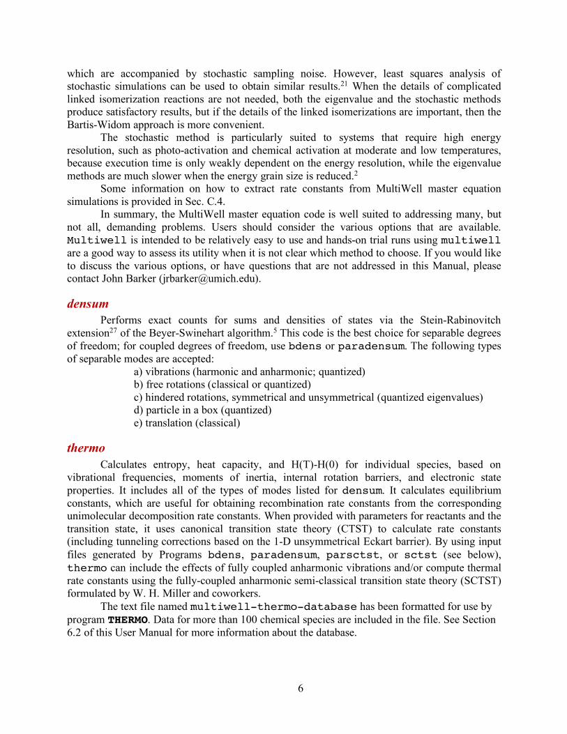
densum Performs exact counts for sums and densities of states via the Stein-Rabinovitch

extension27 of the Beyer-Swinehart algorithm.5 This code is the best choice for separable degrees of freedom; for coupled degrees of freedom, use bdens or paradensum. The following types of separable modes are accepted:

a) vibrations (harmonic and anharmonic; quantized) b) free rotations (classical or quantized) c) hindered rotations, symmetrical and unsymmetrical (quantized eigenvalues) d) particle in a box (quantized) e) translation (classical)

thermo Calculates entropy, heat capacity, and H(T)-H(0) for individual species, based on

vibrational frequencies, moments of inertia, internal rotation barriers, and electronic state properties. It includes all of the types of modes listed for densum. It calculates equilibrium constants, which are useful for obtaining recombination rate constants from the corresponding unimolecular decomposition rate constants. When provided with parameters for reactants and the transition state, it uses canonical transition state theory (CTST) to calculate rate constants (including tunneling corrections based on the 1-D unsymmetrical Eckart barrier). By using input files generated by Programs bdens, paradensum, parsctst, or sctst (see below), thermo can include the effects of fully coupled anharmonic vibrations and/or compute thermal rate constants using the fully-coupled anharmonic semi-classical transition state theory (SCTST) formulated by W. H. Miller and coworkers.

The text file named multiwell-thermo-database has been formatted for use by program THERMO. Data for more than 100 chemical species are included in the file. See Section 6.2 of this User Manual for more information about the database.

7

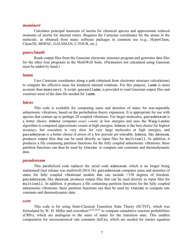
mominert Calculates principal moments of inertia for chemical species and approximate reduced

moments of inertia for internal rotors. Requires the Cartesian coordinates for the atoms in the molecule, as obtained from many software packages in common use (e.g., HyperChem, Chem3D, MOPAC, GAUSSIAN, C-FOUR, etc.).

gauss2multi Reads output files from the Gaussian electronic structure program and generates data files

for the other four programs in the MultiWell Suite. (Parameters not calculated using Gaussian must be added by hand.)

lamm Uses Cartesian coordinates along a path (obtained from electronic structure calculations)

to compute the effective mass for hindered internal rotations. For this purpose, lamm is more accurate than mominert. A script, gauss2lamm, is provided to read Gaussian output files and construct most of the data file needed for lamm.

bdens This code is available for computing sums and densities of states for non-separable

anharmonic vibrations, based on the perturbation theory expansion. It is appropriate for use with species that contain up to perhaps 20 coupled vibrations. For larger molecules, paradensum is a better choice. bdens computes exact counts at low energies and uses the Wang-Landau algorithm to computed approximate counts at high energies. bdens is the best choice for highest accuracy, but execution is very slow for very large molecules at high energies, and paradensum is a better choice if errors of a few percent are tolerable. bdens, like densum, produces output files that can be used directly as input files for multiwell. In addition, it produces a file containing partition functions for the fully coupled anharmonic vibrations; these partition functions can then be used by thermo to compute rate constants and thermodynamic data.

paradensum This parallelized code replaces the serial code adensum, which is no longer being

maintained (last release was multiwell-2014.1b). paradensum computes sums and densities of states for fully coupled vibrational models that can include >150 degrees of freedom. paradensum, like densum, produces output files that can be used directly as input files for multiwell. In addition, it produces a file containing partition functions for the fully coupled anharmonic vibrations; these partition functions can then be used by thermo to compute rate constants and thermodynamic data.

sctst This code is for using Semi-Classical Transition State Theory (SCTST), which was

formulated by W. H. Miller and coworkers14,22,24,25 to compute cumulative reaction probabilities (CRPs), which are analogous to the sums of states for the transition state. This enables computation for microcanonical rate constants (k(E)s), which are needed for master equation

8

simulations (using multiwell). Miller's theory is founded on second order vibrational perturbation theory (VPT2). An additional feature of the code is the implementation of J. F. Stanton's additional correction term, which is based on fourth-order perturbation vibrational theory (VPT4). The code also computes the partition function corresponding to the CRP at a set of temperatures from 50 K to 3400 K and generates a data file that can be used by program thermo to conveniently compute thermal rate constants using SCTST.

parsctst This code is the parallel version of sctst. It can also be run as a serial code and will

replace sctst in a future release. It is for using Semi-Classical Transition State Theory (SCTST), which was formulated by W. H. Miller and coworkers14,22,24,25 to compute cumulative reaction probabilities (CRPs), which are analogous to the sums of states for the transition state. This enables computation for microcanonical rate constants (k(E)s), which are needed for master equation simulations (using multiwell). Miller's theory is founded on second order vibrational perturbation theory (VPT2). An additional feature of the code is the implementation of J. F. Stanton's additional correction term, which is based on fourth-order perturbation vibrational theory (VPT4). The code also computes the partition function corresponding to the CRP at a set of temperatures from 50 K to 3400 K and generates a data file that can be used by program thermo to conveniently compute thermal rate constants using SCTST.

ktools This code implements two varieties of Variational Transition State Theory (VTST):

Canonical (i.e. thermal) and J-resolved Microcanonical (i.e. for fixed internal energies and angular momentum). From molecular vibration frequencies, moments of inertia, and potential energy provided at points along a reaction path to compute variationally optimized sums of states and J-resolved microcanonical rate constants (i.e. k(E,J)) for the reaction. These quantities can be used in 2-dimensional (i.e. depending on both E and J) master equations. By summing over J, it also gives microcanonical VTST rate constants (i.e. k(E) that can be used in 1-D (i.e. depending on E, alone) master equations. An important feature otf the code is that it automatically identifies cases where two or more bottlenecks occur along the same reaction path and then uses W. H. Miller's unified statistical theory23 to compute the over-all effective rae constant.

TS This code features a J-resolved steady-state master equation code that is solved by

eigenvalue methods on large parallel computers. It utilizes the frozen-J approximation.

9

1.2 How the Tools Work Together In this section, we describe the input and output of codes in the MultiWell Program Suite

and indicate how some codes generate output files that are used as input by other codes. In the following table, <species> denotes the name of a chemical species (i.e. a Well or a Transition State).

Table 1. Software Tools Input/Output Information

Tool Input Quantities Output thermo (Chap. 6)

Separable D.O.F. (Chap. 3) Vibrations Rotations Hindered rotors etc. Electronic energies Symmetries

Heat Capacity Entropy Enthalpy function Equilibrium Const. Canonical (Thermal) Rate Constants

Input Files Description Generated by… thermo.dat

<species>.qvib <species>.crp

data file (required) Partition functions Partition functions Cumulative React. Probability

User bdens paradensum sctst parsctst

Output Files Description used by program… thermo.out

thermo.partfxns thermo.details

General output Partition functions Details

(none)

Tool Input Quantities Output densum (Chap. 4)

Separable D.O.F. (Chap. 3) Vibrations Rotations Hindered rotors etc.

G(E), sum of states ρ(E), density of states

Input Files Description Generated by… densum.dat

data file (required) User

Output Files Description used by program… densum.out

<species>.dens

General output G(E) and ρ(E)

User multiwell

10

Tool Input Quantities Output multiwell (Chap. 2) Master equation simulations.

Cartesian coordinates Fractional concentrations vs. time.

Branching fractions, internal energies, etc.

Input Files Description Generated by… multiwell.dat

<species name>.dens <TS name>.crp (other optional

input files)

data file (required) Sums and densities of states Cumulative Reaction

probabilities k(E), initial energy distributions,

etc.

User densum, ktools, paradensum, bdens

sctst User

Output Files Description used by program… multiwell.out

multiwell.sum multiwell.array multiwell.rates multiwell.flux multiwell.dist

General output Output summary Input and meta data Reaction flux coefficients Reactive fluxes Energy distributions

Tool Input Quantities Output mominert (Chap. 5)

Cartesian coordinates External moments of inertia and rotational constants

Reduced moment of inertia and rotational constants for internal rotors

Input Files Description Generated by… mominert.dat

data file (required)

User

Output Files Description used by program… mominert.out

General output

input data used by many of the other codes

Tool Input Quantities Output lamm (Chap. 9)

Cartesian coordinates as a function of dihedral angle for an internal rotation.

Reduced moment of inertia and rotational constant as a function of dihedral angle

Input Files Description Generated by… lamm.dat

data file (required)

User

Output Files Description used by program… lamm.out

General output

thermo densum bdens paradensum sctst parsctst ktools

11

Tool Input Quantities Output ktools (Chap. 10) J-Resolved VTST code

For a Transition State Separable D.O.F. (Chap. 3) Vibrations Rotations Hindered rotors etc. Electronic energies Symmetries

Canonical k(T) and J-resolved microcanonical k(E,J) VTST rate constants; also J-resolved sums G(E,J) and densities ρ(E,J) of states; also J-summed quantities.

Input Files Description Generated by… ktools.dat


Output Files Description used by …

Tool Input Quantities Output bdens (Chap. 8) Fully coupled vibrational models for small species.

Coupled vibrations (Chap. 8) Harmonic frequencies Anharmonicities (Xij) Separable D.O.F. (Chap. 3) Vibrations Rotations Hindered rotors etc.

G(E), sum of states ρ(E), density of states partition functions

Input Files Description Generated by… bdens.dat


Output Files Description used by program… bdens.out

<species>.dens <species>.qvib

General output G(E) and ρ(E)s Partition functions

User multiwell thermo

Tool Input Quantities Output paradensum (Chap. 8) Fully coupled vibrational models for large species.

Coupled vibrations (Chap. 8) Harmonic frequencies Anharmonicities (Xij) Separable D.O.F. (Chap. 3) Vibrations Rotations Hindered rotors, etc.

G(E), sum of states ρ(E), density of states partition functions

Input Files Description Generated by… paradensum.dat


Output Files Description used by … paradensum.out

<species>.dens <species>.qvib

General output G(E) and ρ(E) Partition functions


12

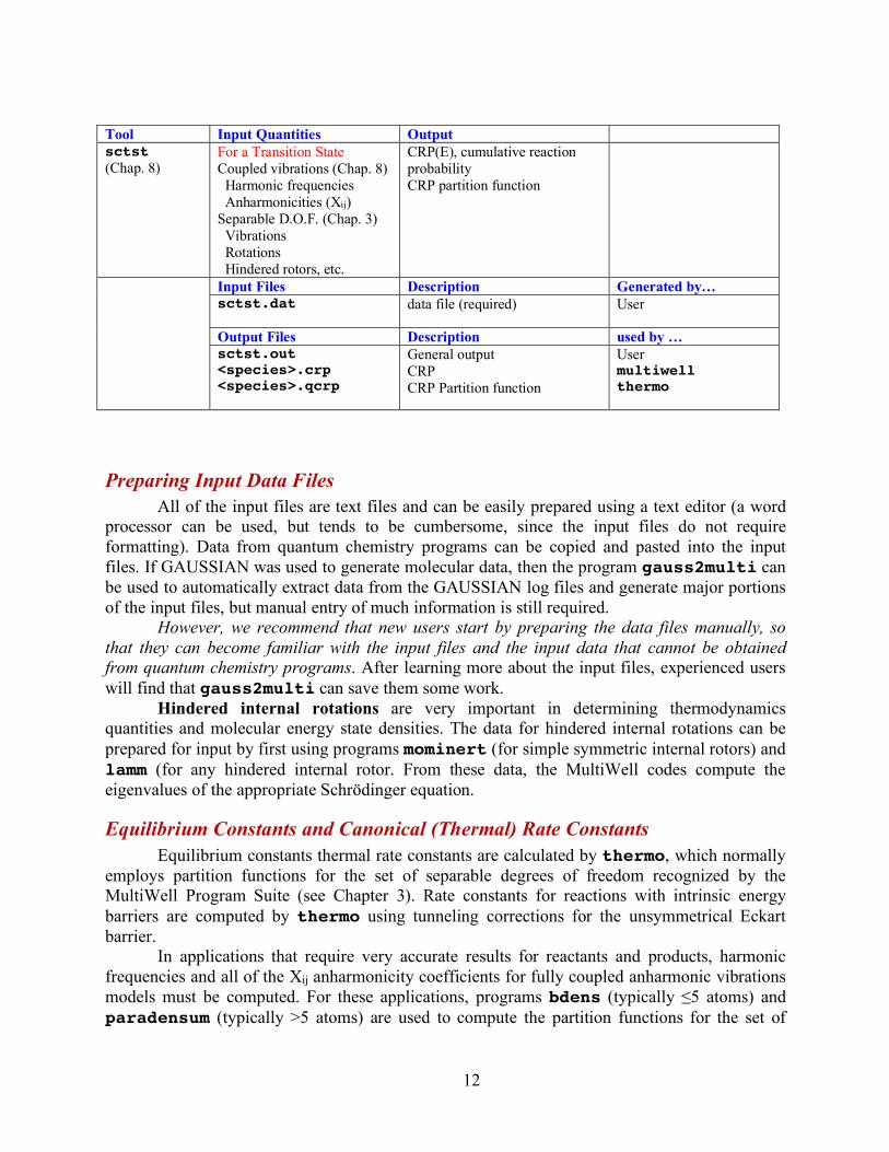
Tool Input Quantities Output sctst (Chap. 8)

For a Transition State Coupled vibrations (Chap. 8) Harmonic frequencies Anharmonicities (Xij) Separable D.O.F. (Chap. 3) Vibrations Rotations Hindered rotors, etc.

CRP(E), cumulative reaction probability CRP partition function

Input Files Description Generated by… sctst.dat


Output Files Description used by … sctst.out

<species>.crp <species>.qcrp

General output CRP CRP Partition function


Preparing Input Data Files All of the input files are text files and can be easily prepared using a text editor (a word

processor can be used, but tends to be cumbersome, since the input files do not require formatting). Data from quantum chemistry programs can be copied and pasted into the input files. If GAUSSIAN was used to generate molecular data, then the program gauss2multi can be used to automatically extract data from the GAUSSIAN log files and generate major portions of the input files, but manual entry of much information is still required.

However, we recommend that new users start by preparing the data files manually, so that they can become familiar with the input files and the input data that cannot be obtained from quantum chemistry programs. After learning more about the input files, experienced users will find that gauss2multi can save them some work.

Hindered internal rotations are very important in determining thermodynamics quantities and molecular energy state densities. The data for hindered internal rotations can be prepared for input by first using programs mominert (for simple symmetric internal rotors) and lamm (for any hindered internal rotor. From these data, the MultiWell codes compute the eigenvalues of the appropriate Schrödinger equation.

Equilibrium Constants and Canonical (Thermal) Rate Constants Equilibrium constants thermal rate constants are calculated by thermo, which normally

employs partition functions for the set of separable degrees of freedom recognized by the MultiWell Program Suite (see Chapter 3). Rate constants for reactions with intrinsic energy barriers are computed by thermo using tunneling corrections for the unsymmetrical Eckart barrier.

In applications that require very accurate results for reactants and products, harmonic frequencies and all of the Xij anharmonicity coefficients for fully coupled anharmonic vibrations models must be computed. For these applications, programs bdens (typically ≤5 atoms) and paradensum (typically >5 atoms) are used to compute the partition functions for the set of

13

coupled vibrations; these two programs generate output files that can be read as input to thermo.

For tight transition states (i.e. with intrinsic energy barriers) with fully-coupled vibrations (including the reaction coordinate), program parsctst (or sctst) calculates the cumulative reaction probability (CRP) and appropriate partition functions, which are placed in an output file that can be read as input to thermo.

For loose transition states (i.e. with little or no intrinsic energy barriers), program ktools is appropriate. This code utilizes separable degrees of freedom and information at points along the reaction path. It automatically identifies situations with multiple transition states along the reaction path and computes the net rate constant.

RRKM Master Equation Calculations These calcualtions are performed using multiwell, the master equation code.

multiwell has a standard input file for many of the required parameters, but it also requires densities of states for Wells and sums of states for Transition States. For standard calculations that adopt separable degrees of freedom, the densities of states for the Wells are computed using densum. For tight Transition States, densum is appropriate, but for loose Transition States, ktools is the proper choice.

For applications that use fully coupled vibrations, bdens and paradensum can be used to calculate the densities of states for the Wells and parsctst (or sctst) can be used for the Transition States; these programs generate output files that can be read by multiwell.

1.3 Examples and Models

Examples Several examples are provided for each of the codes: multiwell, densum,

mominert, thermo, gauss2multi, ktools, bdens, paradensum, sctst, and parsctst. The densum examples include a set of cases discussed in the literature: useful for testing the accuracy of densum. The multiwell examples include various reaction Models.

The input files found in the Examples can be used as templates to construct new input files. Example input files can also be found in the "test" directories, which are located in each source (src) directory (see section 1.4 for the directory structure).

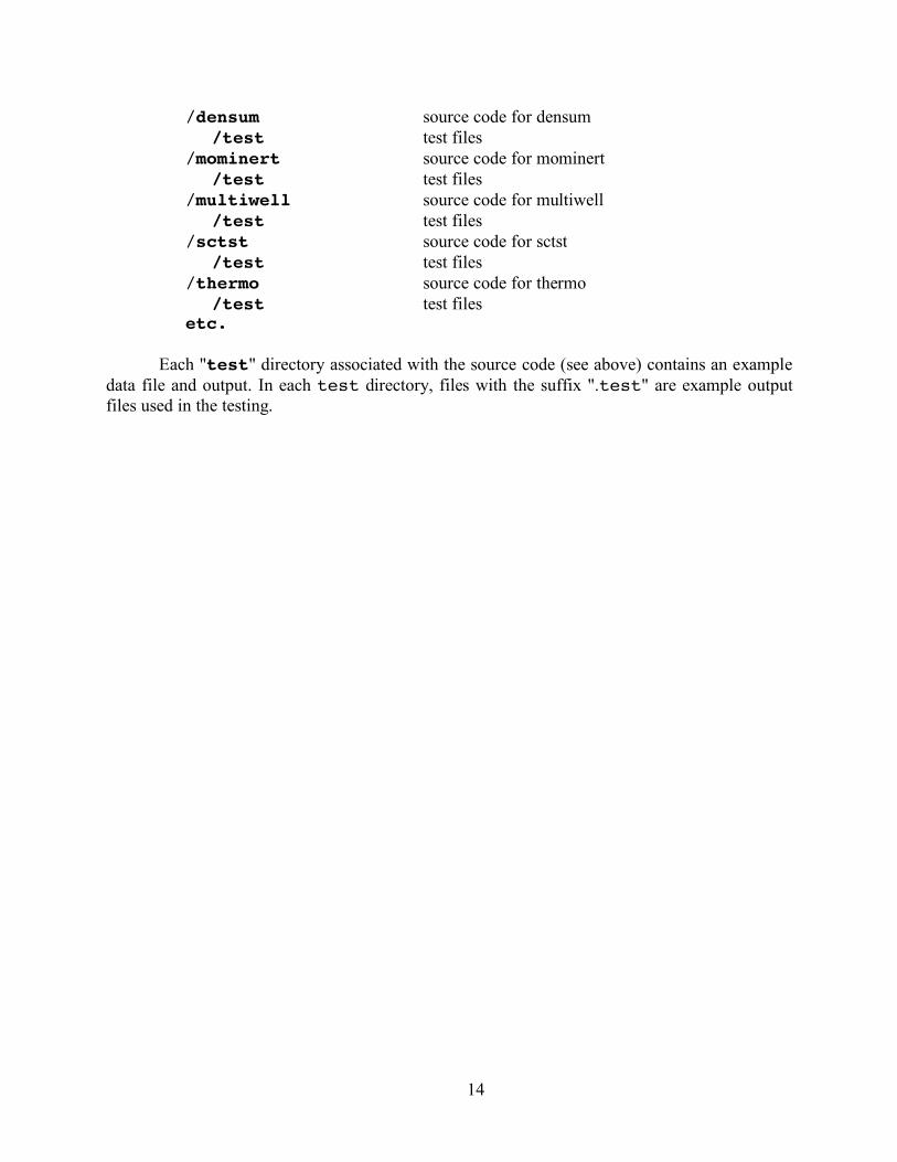
The MultiWell Software Suite directory is organized as follows:

/multiwell-<version> Main MultiWell Directory /bin binary executables /doc version history, license, etc. /scripts admin scripts for running tests and examples /src /bdens source code for bdens /test test files for densum] /test test files /gauss2multi source code for gauss2multi /test [test files for densum] /test test files

14

/densum source code for densum /test [test files for densum] /test test files /mominert source code for mominert /test [test files for mominert] /test test files /multiwell source code for multiwell /test test files /sctst source code for sctst /test test files /thermo source code for thermo /test test files etc.

Each "test" directory associated with the source code (see above) contains an example

data file and output. In each test directory, files with the suffix ".test" are example output files used in the testing.

15

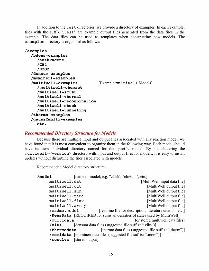
In addition to the test directories, we provide a directory of examples. In each example, files with the suffix ".test" are example output files generated from the data files in the example. The data files can be used as templates when constructing new models. The examples directory is organized as follows:

/examples /bdens-examples /anthracene /CH4 /H2O2 /densum-examples /mominert-examples /multiwell-examples [Example multiwell Models] / multiwell-chemact /multiwell-sctst /multiwell-thermal /multiwell-recombination /multiwell-shock /multiwell-tunneling /thermo-examples /gauss2multi-examples etc.

Recommended Directory Structure for Models Because there are multiple input and output files associated with any reaction model, we

have found that it is most convenient to organize them in the following way. Each model should have its own individual directory named for the specific model. By not cluttering the multiwell-<version> directory with input and output files for models, it is easy to install updates without disturbing the files associated with models.

Recommended Model directory structure: /model [name of model; e.g. "c2h6", "clo+clo", etc.] multiwell.dat [MultiWell input data file] multiwell.out [MultiWell output file] multiwell.sum [MultiWell output file] multiwell.rate [MultiWell output file] multiwell.flux [MultiWell output file] multiwell.array [MultiWell output file] readme.model [read-me file for description, literature citation, etc.] /DensData [REQUIRED for sums an densities of states used by MultiWell] /multidata [for stored multiwell data files] /vibs [densum data files (suggested file suffix: “.vibs”)] /thermodata [thermo data files (suggested file suffix: “.therm”)] /momidata [mominert data files (suggested file suffix: “.mom”)] /results [stored output]

16

1.4 Installing and Executing the Codes

Linux/Unix (and Mac OS X) Versions

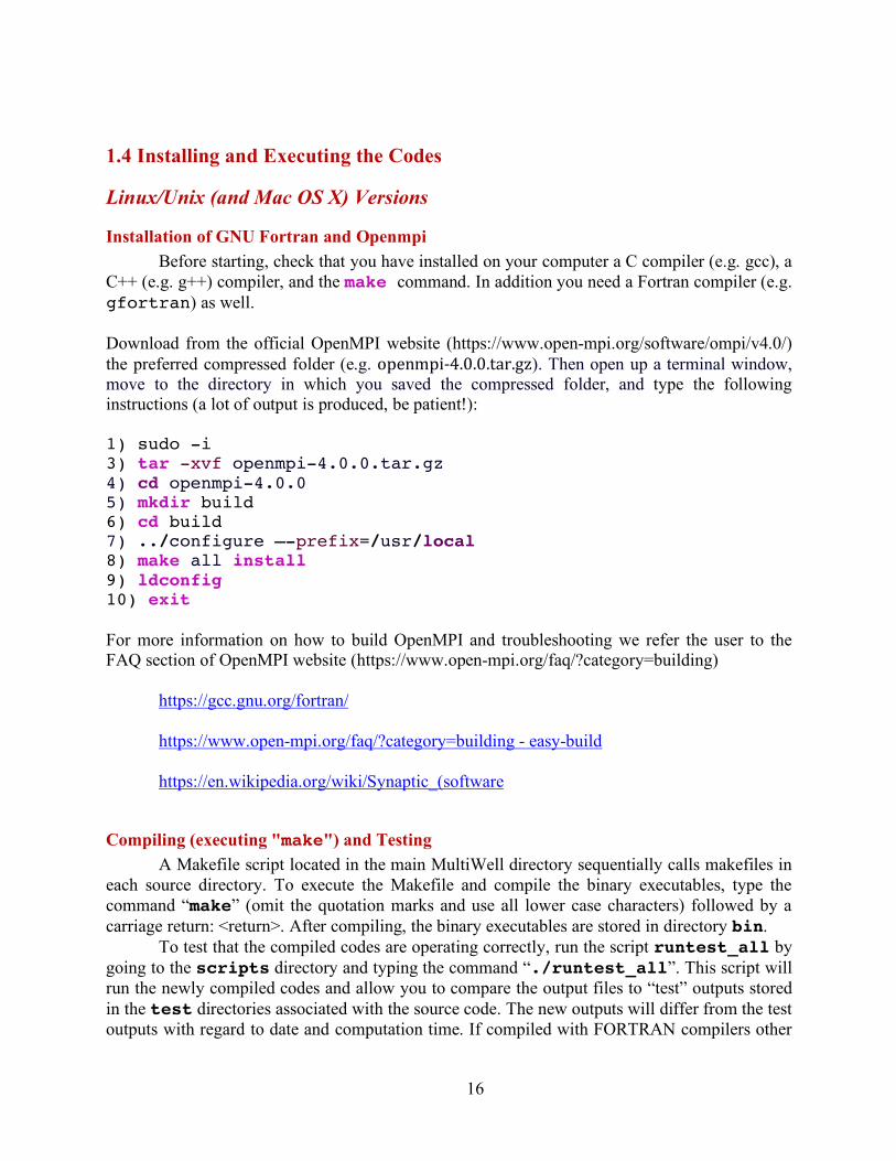
Installation of GNU Fortran and Openmpi Before starting, check that you have installed on your computer a C compiler (e.g. gcc), a

C++ (e.g. g++) compiler, and the make command. In addition you need a Fortran compiler (e.g. gfortran) as well. Download from the official OpenMPI website (https://www.open-mpi.org/software/ompi/v4.0/) the preferred compressed folder (e.g. openmpi-4.0.0.tar.gz). Then open up a terminal window, move to the directory in which you saved the compressed folder, and type the following instructions (a lot of output is produced, be patient!): 1) sudo -i 3) tar -xvf openmpi-4.0.0.tar.gz 4) cd openmpi-4.0.0 5) mkdir build 6) cd build 7) ../configure –-prefix=/usr/local 8) make all install 9) ldconfig 10) exit For more information on how to build OpenMPI and troubleshooting we refer the user to the FAQ section of OpenMPI website (https://www.open-mpi.org/faq/?category=building)

https://gcc.gnu.org/fortran/ https://www.open-mpi.org/faq/?category=building - easy-build https://en.wikipedia.org/wiki/Synaptic_(software

Compiling (executing "make") and Testing A Makefile script located in the main MultiWell directory sequentially calls makefiles in

each source directory. To execute the Makefile and compile the binary executables, type the command “make” (omit the quotation marks and use all lower case characters) followed by a carriage return: <return>. After compiling, the binary executables are stored in directory bin.

To test that the compiled codes are operating correctly, run the script runtest_all by going to the scripts directory and typing the command “./runtest_all”. This script will run the newly compiled codes and allow you to compare the output files to “test” outputs stored in the test directories associated with the source code. The new outputs will differ from the test outputs with regard to date and computation time. If compiled with FORTRAN compilers other

17

than GNU Fortran, there may be minor numerical differences. If significant differences appear, then it is possible that the compiled codes are not working properly.

It is highly recommended that users do not place user data files, etc., in directory /multiwell-<version> (see Section 1.3) Instead, users should create individual directories for user models (see Section 1.5) and execute MultiWell from within those directories. This approach makes it very easy to replace the entire directory /multiwell-<version> with a newer version. Programs in the MultiWell Suite are executed as described in Section 2.5.

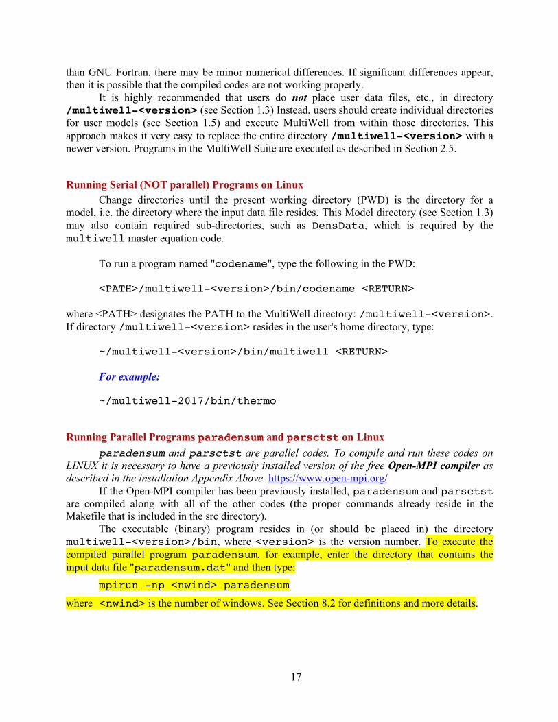
Running Serial (NOT parallel) Programs on Linux Change directories until the present working directory (PWD) is the directory for a

model, i.e. the directory where the input data file resides. This Model directory (see Section 1.3) may also contain required sub-directories, such as DensData, which is required by the multiwell master equation code.

To run a program named "codename", type the following in the PWD: <PATH>/multiwell-<version>/bin/codename <RETURN>

where <PATH> designates the PATH to the MultiWell directory: /multiwell-<version>. If directory /multiwell-<version> resides in the user's home directory, type:

~/multiwell-<version>/bin/multiwell <RETURN> For example: ~/multiwell-2017/bin/thermo

Running Parallel Programs paradensum and parsctst on Linux paradensum and parsctst are parallel codes. To compile and run these codes on

LINUX it is necessary to have a previously installed version of the free Open-MPI compiler as described in the installation Appendix Above. https://www.open-mpi.org/

If the Open-MPI compiler has been previously installed, paradensum and parsctst are compiled along with all of the other codes (the proper commands already reside in the Makefile that is included in the src directory).

The executable (binary) program resides in (or should be placed in) the directory multiwell-<version>/bin, where <version> is the version number. To execute the compiled parallel program paradensum, for example, enter the directory that contains the input data file "paradensum.dat" and then type:

mpirun -np <nwind> paradensum

where <nwind> is the number of windows. See Section 8.2 for definitions and more details.

18

Windows Versions In the Windows version, binary executables (application, or .EXE files) have already

been compiled and are found in the sub-directory "multiwell-<version>/bin".

Running Serial (NOT Parallel) Programs on Windows To run any of the programs in the MultiWell Suite, except for parallel codes like

paradensum and parsctst (for parallel codes, see below), the steps are as follows:

1. Prepare a data file (for instructions, see the User Manual and the Examples directory) and place it in a directory devoted to your Model (see Section 1.3). This "Model" directory may also contain required sub-directories, such as DensData, which is required by the multiwell master equation code.

2. Change directories until the present working directory (PWD) is the directory for a model, i.e. the directory where the input data file resides. For densum calculations, for example, the data file (densum.dat) may reside in the directory Model/vibs.

3. Create an alias of the executable of interest (e.g. densum.exe) and place the alias in the Model directory (folder) as the data file. For densum calculations, for example, if the data file densum.dat resides in the directory Model/vibs, the alias should also be placed in directory Model/vibs.

4. Double-click the alias. The output files (e.g. densum.out, etc.) will be written to the same directory.

Expert Users Expert Users can set the PATH in Windows and run all of the programs, except for

paradensum and parsctst, in a DOS window. From the Model directory where the input data file resides, type: <PATH>/multiwell-<version>/bin/densum.exe <RETURN> For example: ~/multiwell-2017/bin/densum.exe

Running Parallel Programs paradensum and parsctst on Windows

Installation 1. The paradensum and parsctst versions for Windows can be downloaded as a precompiled

executable files paradensum.exe and parsctst.exe. 2. These are parallel codes. To properly run parallel codes it is necessary to have a previously

19

installed version of Microsoft MPI implementation. To download the Microsoft MPI, the reader is referred to the website:

https://www.microsoft.com/en-us/download/details.aspx?id=56727

Download both msmpisdk.msi and MSMpiSetup.exe and execute them.

Execution

1. Put the paradensum.exe or the parsctst.exe executable and parameters.dat input data file in the Model directory.

2. Open the Windows Command Prompt and change directory to the folder that contains paradensum.exe or the parsctst.exe. To run the code with the selected number of windows <nwind>, type:

mpiexec -n <nwind> paradensum.exe or

mpiexec -n <nwind> parsctst.exe 3. All of the output files are automatically generated in the same folder.

1.5 Some Technical Issues on Input/Output Files All input and output files are text. Input files can be created using almost any text editor

that generates unformatted text files. For ease of reading the output files, do not use word-wrapping.

When compiled using GNU and Open-MPI compilers, the following constructs are

allowed in the text datafiles (they may, or may not, be permitted when the codes are compiled using other compilers):

• Numerical entries can be separated by commas, blanks, tabs, and line returns. • Blank lines are ignored. • In most cases, end of line comments can be entered following a "!" symbol. • Character variables may be enclosed in a matched pair of 'single quotation marks', or

"double-quotation marks". Often, character variables that are single words do not require any quotes if separated from other entries by tabs, blanks, or line returns. When in doubt, enclose them in a matched pair of quotes.

• Title lines are separated from other entries by line returns.

20

References

(1) Andraos, J. A Streamlined Approach to Solving Simple and Complex Kinetic Systems

Analytically. J. Chem. Educ. 1999, 76, 1578-1583; DOI: 10.1021/ed076p1578. (2) Barker, J. R.; Frenklach, M.; Golden, D. M. Reply to “Comment on ‘When Rate

Constants Are Not Enough’”. J. Phys. Chem. A 2016, 120, 313−317; DOI: 10.1021/acs.jpca.5b06652.

(3) Barker, J. R.; Stimac, P. J.; King, K. D.; Leitner, D. M. CF3CH3 → HF + CF2CH2: A non-RRKM Reaction? J. Phys. Chem. A 2006, 110, 2944-2954; 10.1021/jp054510x.

(4) Bartis, J. T.; Widom, B. Stochastic models of the interconversion of three or more chemical species. J. Chem. Phys. 1974, 60, 3474-3482; doi: 10.1063/1.1681562.

(5) Beyer, T.; Swinehart, D. F. Number of multiply-restricted partitions. Comm. Assoc. Comput. Machines 1973, 16, 379.

(6) Boyd, S.; Vandenberghe, L. Convex Optimization; Cambridge University Press: Cambridge, UK, 2004.

(7) Duong, M. V.; Nguyen, H. T.; Truong, N.; Le, T. N. M.; Huynh, L. K. Multi-Species Multi-Channel (MSMC): An Ab Initio-based Parallel Thermodynamic and Kinetic Code for Complex Chemical Systems. International Journal of Chemical Kinetics 2015, 47, 564-575; doi: 10.1002/kin.20930.

(8) Frenklach, M.; Packard, A.; Feeley, R. Optimization of Reaction Models with Solution Mapping. In Modeling of Chemical Reactions; Carr, R. W., Ed.; Elsevier: Amsterdam, 2007; Vol. 42; pp 243–291.

(9) Gillespie, D. T. A general method for numerically simulating the stochastic time evolution of coupled chemical reactions. J. Comp. Phys. 1976, 22, 403-434.

(10) Gillespie, D. T. Exact stochastic simulation of coupled chemical reactions. J. Phys. Chem. 1977, 81, 2340-2361.

(11) Gillespie, D. T. A rigorous derivation of the chemical master equation. Physica A: Statistical and Theoretical Physics (Amsterdam) 1992, 188, 404-425.

(12) Glowacki, D. R.; Liang, C. H.; Morley, C.; Pilling, M. J.; Robertson, S. H. MESMER: An Open-Source Master Equation Solver for Multi-Energy Well Reactions. J. Phys. Chem. A 2012, 116, 9545-9560; 10.1021/jp3051033.

(13) Gruebele, M.; Wolynes, P. G. Vibrational energy flow and chemical reactions. Accounts of Chemical Research 2004, 37, 261-267.

(14) Hernandez, R.; Miller, W. H. Semiclassical transition state theory. Chem. Phys. Lett. 1993, 214, 129-136.

(15) Leitner, D. M. Heat Transport in Molecules and Chemical Kinetics: The Role of Quantum Energy Flow and Localization. In Geometric Structures of Phase Space in Multi-Dimensional Chaos: Applications to Chemical Reaction Dynamics in Complex Systems, Adv. Chem. Phys., vol. 130 (Part B); Toda, M., Komatsuzaki, T., Konishi, T., Rice, S. A., Berry, R. S., Eds.; Wiley, 2005; Vol. 130 (Part B); pp 205-256.

(16) Leitner, D. M.; Levine, B.; Quenneville, J.; Martinez, T. J.; Wolynes, P. G. Quantum energy flow and trans-stilbene photoisomerization: an example of a non-RRKM reaction. Journal of Physical Chemistry A 2003, 107, 10706-10716.

21

(17) Leitner, D. M.; Wolynes, P. G. Many-dimensional quantum energy flow at low energy. Phys. Rev. Lett. 1996, 76, 216-219.

(18) Leitner, D. M.; Wolynes, P. G. Quantum energy flow during molecular isomerization. Chemical Physics Letters 1997, 280, 411-418.

(19) Lewis, E. S.; Johnson, M. D. The Reactions of p-Phenylene-bis-diazonium Ion with Water. J. Am. Chem. Soc. 1960, 82, 5399–5407; DOI: 10.1021/ja01505a027.

(20) Miller, J. A.; Klippenstein, S. J. Master Equation Methods in Gas Phase Chemical Kinetics. J. Phys. Chem. A 2006, 110, 10528-10544.

(21) Miller, J. A.; Klippenstein, S. J.; Robertson, S. H.; Pilling, M. J.; Shannon, R.; Zádor, J.; Jasper, A. W.; Goldsmith, C. F.; Burke, M. P. Comment on “When Rate Constants Are Not Enough”. J. Phys. Chem. A 2016, 120, 306−312; DOI: 10.1021/acs.jpca.5b06025.

(22) Miller, W. H. Semiclassical limit of quantum mechanical transition state theory for nonseparable systems. J. Chem. Phys. 1975, 62, 1899-1906.

(23) Miller, W. H. Unified statistical model for "complex" and "direct" reaction mechanisms. J. Chem. Phys. 1976, 65, 2216-2223; https://doi.org/10.1063/1.433379.

(24) Miller, W. H. Semi-Classical Theory for Non-separable Systems: Construction of "Good" Action-Angle Variables for Reaction Rate Constants. Faraday Discuss. Chem. Soc. 1977, 62, 40-46.

(25) Miller, W. H.; Hernandez, R.; Handy, N. C.; Jayatilaka, D.; Willetts, A. Ab initio Calculation of Anharmonic Constants for a Transition-State, with Application to Semiclassical Transition-State Tunneling Probabilities. Chemical Physics Letters 1990, 172, 62-68; Doi 10.1016/0009-2614(90)87217-F.

(26) Mucientes, A. E.; Peña, M. A. d. l. Kinetic Analysis of Parallel-Consecutive First-Order Reactions with a Reversible Step: Concentration–Time Integrals Method. J. Chem. Educ. 2009, 86, 390-392; DOI: 10.1021/ed086p390.

(27) Stein, S. E.; Rabinovitch, B. S. Accurate evaluation of internal energy level sums and densities including anharmonic oscillators and hindered rotors. J. Chem. Phys. 1973, 58, 2438-2445.

22

2. MultiWell Master Equation Code Codes, examples, and this manual are available from the MultiWell Program Suite web site: clasp-research.engin.umich.edu/multiwell

2.1 Brief Description MultiWell calculates time-dependent concentrations, yields, vibrational distributions, and

rate constants as functions of temperature and pressure for unimolecular reaction systems which consist of multiple stable species, multiple reaction channels interconnecting them, and multiple dissociation channels from each stable species. The stochastic method is used to solve the resulting Master Equation. Users may supply unimolecular reaction rates, sums of states and densities of states, or optionally use Forst's Inverse Laplace Transform method10-12 to calculate k(E). For weak collisions, users can select from among many collision models, or provide user-defined functions.

The code is intended to be relatively easy to use. It is designed so that very complicated and very simple unimolecular reaction systems can be handled via the data file. Restructuring of the code and recompiling are NOT necessary to handle even the most complex systems.

MultiWell is most suitable for time-dependent non-equilibrium systems. The real time needed for a calculation depends mostly upon the number of collisions during a simulated time period and on the number of stochastic trials needed to achieve the desired precision. For slow reaction rates and precise yields of minor reaction products, the code will require a long run time, but it will produce results. For long calculation runs, we often just let it run overnight.

MultiWell is based on the Gillespie Exact Stochastic algorithm,13-15 as modified and implemented in our laboratory.1,2,5,22 It has been described in considerable detail in a recent publication.3 An example calculation has also been published.6

In the example,6 chemical activation and shock wave simulations were carried out for a system consisting of six isomers and 49 energy-dependent unimolecular reactions. The isomers were interconnected by reversible isomerization reactions, and each isomer could also decompose, resulting in 14 sets of products. Many of the capabilities of MultiWell are illustrated in that paper.6

2.2 Terminology The following sketch shows the potential energy as a function of reaction coordinate for a

typical unimolecular system with multiple wells.

• Wells are chemical species corresponding to local minima on the potential energy surface (PES). They must have at least one bound vibrational state (i.e., at least the zero point, v=0 state). This definition is precise, sufficient, and economical; we do not find it useful to attach any other conditions.

• Transition states for reaction are defined in the usual way. They may be fixed (i.e. associated with a local maximum on the PES), or variational.

• Product sets are the fragmentation products corresponding to irreversible reaction via a given transition state. In this user Manual, Product Sets and Reactant Sets are synonymous, since they refer to the same reaction channel.

23

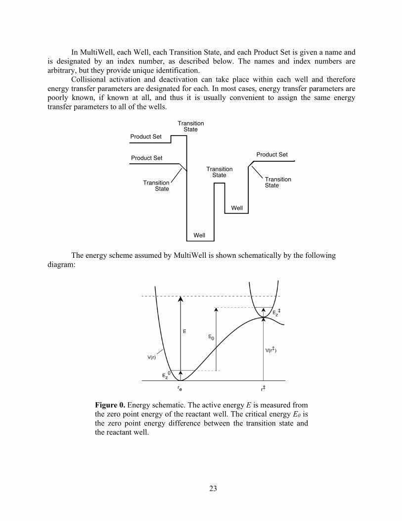
In MultiWell, each Well, each Transition State, and each Product Set is given a name and is designated by an index number, as described below. The names and index numbers are arbitrary, but they provide unique identification.

Collisional activation and deactivation can take place within each well and therefore energy transfer parameters are designated for each. In most cases, energy transfer parameters are poorly known, if known at all, and thus it is usually convenient to assign the same energy transfer parameters to all of the wells.

The energy scheme assumed by MultiWell is shown schematically by the following

diagram:

Figure 0. Energy schematic. The active energy E is measured from the zero point energy of the reactant well. The critical energy E0 is the zero point energy difference between the transition state and the reactant well.

Product Set

Product Set Product Set

TransitionState

TransitionState Transition

StateTransitionState

Well

Well

24

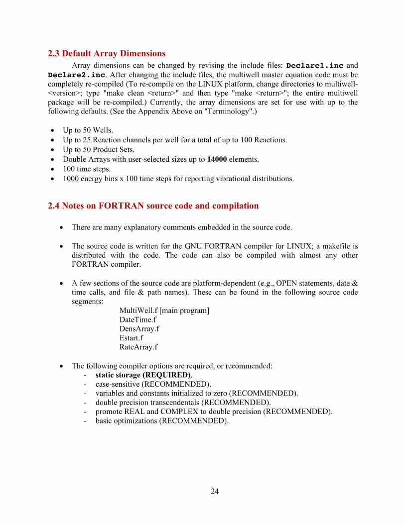
2.3 Default Array Dimensions Array dimensions can be changed by revising the include files: Declare1.inc and

Declare2.inc. After changing the include files, the multiwell master equation code must be completely re-compiled (To re-compile on the LINUX platform, change directories to multiwell-<version>; type "make clean <return>" and then type "make <return>"; the entire multiwell package will be re-compiled.) Currently, the array dimensions are set for use with up to the following defaults. (See the Appendix Above on "Terminology".)

• Up to 50 Wells. • Up to 25 Reaction channels per well for a total of up to 100 Reactions. • Up to 50 Product Sets. • Double Arrays with user-selected sizes up to 14000 elements. • 100 time steps. • 1000 energy bins x 100 time steps for reporting vibrational distributions.

2.4 Notes on FORTRAN source code and compilation

• There are many explanatory comments embedded in the source code.

• The source code is written for the GNU FORTRAN compiler for LINUX; a makefile is distributed with the code. The code can also be compiled with almost any other FORTRAN compiler.

• A few sections of the source code are platform-dependent (e.g., OPEN statements, date & time calls, and file & path names). These can be found in the following source code segments:

MultiWell.f [main program] DateTime.f DensArray.f Estart.f RateArray.f

• The following compiler options are required, or recommended:

- static storage (REQUIRED). - case-sensitive (RECOMMENDED). - variables and constants initialized to zero (RECOMMENDED). - double precision transcendentals (RECOMMENDED). - promote REAL and COMPLEX to double precision (RECOMMENDED). - basic optimizations (RECOMMENDED).

25

2.5 MultiWell Input Files and Program Execution The default input data filename is multiwell.dat (all lower case). Starting with version

2008.1, it is possible to change the input data file name and run multiple sessions in the same directory at the same time, each with a user-selected FileName.

To run MultiWell using the default data filename (multiwell.dat):

LINUX/UNIX: in the directory where the input data file and the auxiliary directory

DensData reside, type: <PATH>/multiwell-<version>/bin/multiwell <RETURN>

where <PATH> designates the PATH to /multiwell-<version>. If directory /multiwell-<version> resides in the user home directory, type:

~/multiwell-<version>/bin/multiwell <RETURN> WINDOWS in a DOS window: in the directory where the input data file and the auxiliary

directory DensData reside, type: <PATH>/multiwell-<version>/bin/multiwell <RETURN> For example: ~/multiwell-2013/bin/multiwell

To run MultiWell using a user-defined filename (FileName.dat):

Follow the same procedures described above, but type: <PATH>/multiwell-<version>/bin/multiwell <FileName> <RETURN>

For example: ~/multiwell-2017/bin/multiwell final.dat All of the resulting output files will take names with the same prefix:

final.out final.sum final.rate final.dist final.flux final.array

26

2.6 MultiWell Output Files Output files with an identical FileName (including the default: 'multiwell') are erased

and written-over for every calculation (for optionally naming of files at run time, see Section 2.5). To be saved, they must be re-named. Use a word processor/editor capable of wide-open (no truncation of lines) output, because the output can be hundreds of characters in width, depending on the number of species and products. In Linux, Xemacs, Emacs, Nedit and other editors are available for this purpose. For Macintosh OS X, "Tex-Edit Plus" (share-ware available at http://www.nearside.com/trans-tex/) and "TextWrangler" (free-ware available at http://www.barebones.com/) are very convenient word processors for text files, although full-featured word processors can be used as well.

FileName.out Time-dependent output of concentrations and average energies. Also includes summaries

of input parameters. The time-dependent quantities are the instantaneous values at the time indicated: they are not averaged over the time interval. Hence, the averages are only over the number of trials.

FileName.sum Summary output file intended for convenient calculations of fall-off curves and other

pressure-dependent quantities. This file gives all of the header material in the full output file, but instead of the time-dependent results, only the final results of each simulation are given in the form of a summary table.

FileName.rate Time-dependent output of average reaction flux coefficients, which vary with time in

non-steady-state systems. (When the energy distributions are independent of time and for the reactions are irreversible, the flux coefficients can be identified with rate constants.) Many trials are needed to accumulate good statistics. To improve statistics, the binned results correspond to the number of visits to the bin (which can be many times larger than the number of trials) and are averaged over the time-bin.

FileName.dist Time-dependent vibrational distributions in Wells (not initial or final products). Only the

non-zero array elements are listed. Many trials are needed to accumulate good statistics. Note that the distributions are normalized according to the number of stochastic trials. Therefore, the sum of the array elements for a chemical species (Well) at a given time is equal to the fractional population of that species at that time. Thus the distributions report not only the relative populations as functions of energy and time, but also the growth and decay of species concentrations.

FileName.array Tabulations of all energy-dependent input data. Includes tables of densities of states,

specific rate constants, collision probabilities and normalization factors, and initial energy distributions.

27

FileName.flux Tabulates the reactive flux via each of the unimolecular channels. The reactive flux is

useful for identifying quasi-equilibrium situations and for tracing chemical pathways.

28

2.7 MultiWell Input Data File (FileName.dat) (See Section 2.5 for optional naming of data files at run time.) The datafile uses free input format. NOTES ON FREE INPUT FORMAT: Fields separated by delimiters. - Standard delimiters on most platforms: commas and spaces. - Additional delimiters acceptable on some platforms: tabs. - CHARACTER constants enclosed in apostrophes (') are accepted on most platforms. Some

platforms will accept CHARACTER constants without their being enclosed in apostrophes, but then they cannot contain any of the delimiter characters.

MULTIWELL MAJOR INPUT OPTIONS 1. Densities of states are read from an external file created by DenSum, or other code. 2. Specific Rate constants: k(E)

a) RRKM theory via sums of states read from an external file (created by DenSum, or other code).

b) k(E) values read from external file. c) Reversible and/or irreversible reactions.

3. Initial energy distributions: a) thermal (with an optional energy offset), calculated internally. b) chemical activation, calculated internally. c) delta function d) distribution can be read from an external file.

4. Separate initial vibrational temperature and translational temperature. 5. Can incorporate the effects of slow intramolecular vibrational energy redistribution (IVR). 6. Can include tunneling via an unsymmetrical Eckart barrier.

29

MULTIWELL INPUT DATA FILE FORMAT Note: Starting with version 2.0, the data file format is no longer compatible with previous versions.

PART A: PHYSICAL PARAMETERS

Line 1 (line count ignores blank lines following TITLE) TITLE (up to 100 characters) Line 2 Egrain1, imax1, Isize , Emax2, IDUM

Egrain1 energy grain size of first segment in "double arrays", see Note (units: cm-1) imax1 size of first segment of double array; selected so that sums or densities of states is

a smooth function of energy (less than ~1% relative fluctuations). Note that imax1 must be less than Isize.

Isize user-selected size of double array. The Default array size starting in version 2.08 is set for a maximum of 14000 elements in the INCLUDE file "declare1.inc". (The array size is defined by Imax=14000 in declare1.inc.) This large maximum array size allows users to select any value of Isize ≤ 14000 elements without having to recompile the code. If array sizes greater than 14000 elements are needed, the Imax can be changed in the Linux/Unix version by deleting old object files (by typing ‘make clean’ in /multiwell/src/multiwell) and then recompiling (by typing ‘make’).

Emax2 maximum energy of 2nd segment of double arrays (units: cm-1) IDUM random number seed (integer); EXAMPLE: "2113989025"

***** NOTE: "Double arrays" have two sections: segment 1 consists of imax1 equally spaced (Egrain1) data ranging from E=0; segment 2 consists of equally spaced values from E=0 to Emax2; the size of the second segment is (Isize - imax1); the energy grain of the second segment is Emax2/(Isize - imax1 - 1).

(Appendix A, continued...)

30

Line 3 Punits, Eunits, Rotatunits [It is required that the three keywords be entered in this exact order!]

Punits one of the following pressure units keywords: 'BAR', 'ATM', or 'MCC'[for molecules/cc] (Note that 'TOR' is no longer

accepted.) Eunits one of the following energy units keywords: 'CM-1', 'KCAL', or 'KJOU' for cm-1, kcal/mole or kJ/mole Rotatunits one of the following keywords for rotational information (upper or lower case): 'AMUA', 'GMCM', 'CM-1', 'MHZ', 'GHZ'(for moments of inertia in units of

amu.Å2 or g.cm2, and rotational constants in units of cm-1. MHz, or GHz) Line 4 Temp , Tvib

Temp translational temperature (units: Kelvin) Tvib initial vibrational temperature (units: Kelvin)

For shock-tube simulations, Temp is set equal to the shock (translational) temperature and Tvib is set equal to the vibrational temperature prior to the shock (usually room temperature).

Line 5 Np number of pressures Line 6 PP(1), PP(2), ..., PP(Np) List of Np pressures

31

PART B: PARAMETERS FOR WELLS AND FOR PRODUCT SETS

Line 7 NWells , NProds

NWells number of "wells" (includes irreversible product sets) NProds number of entrance/exit channels; each channel has a product set associated with

it.

Line 8 IMol , MolName , HMol , MolMom , Molsym , Molele , Molopt (REPEAT NWells times: once for each well.)

IMol index number for well (1 ... NWells) MolName name of well (≤10 characters) HMol enthalpy of formation at 0 K (units defined by keyword) MolMom rotational parameter for 2-dimensional external rotation (moment of inertia or

rotational constant; units defined by keyword on Line 3) Molsym external symmetry number for well (see Appendices B4 and B.5) Molele electronic partition function for well (REAL number); depends on temperature;

can be obtained from THERMO output. Molopt number of chiral stereoisomers (or "optical isomers", or mirror images) for well

(see Appendix B.5)

See Appendices B.4 and B.5 for a discussion of proper input for External Molecular Rotations and number of "optical isomers" (i.e. mirror images).

Line 9 IMol , MolName , Hmol (REPEAT NProds times: once for each entrance/exit channel, i.e. for each product set.)

IMol index for channel (NWells+1...NWells+NProds) MolName name of Product set (max 10 characters) Hmol enthalpy of formation at 0 K (units defined by keyword on Line 3) [ignored unless

tunneling is used] ***** NOTE: the numbering of entrance/exit channels starts with NWells+1.

Line 10 SigM, EpsM, AmuM, Amu

32

SigM Lennard-Jones s (Å) for collider EpsM Lennard-Jones e/kB (Kelvins) for collider AmuM Molecular weight (g/mole) of collider Amu Molecular weight (g/mole) of reactant Optional Line 10a OLDET To change the default treatment of collisional energy transfer from Barker's "New

Approach" (see Ref. 4) to the traditional approach, insert the keyword OLDET (upper or lower case) on a new line. The "New Approach" (the default) attenuates the inelastic collision frequency (and hence the rate of inelastic energy transfer) at low energies, where the densities of states are very sparse. The traditional method was based on the convenient assumption that the inelastic collision frequency is independent of internal energy. This feature facilitates intercomparisons between multiwell and other master equation codes.

Line 11 Mol, Sig, Eps, ITYPE, DC(1), DC(2), ... , DC(8) (REPEAT Lines 11 and 12 NWells times: once for each well.)

Mol index number of Well Sig Lennard-Jones s (Å) for this well Eps Lennard-Jones e/kB (Kelvins) for this well ITYPE selects model type in Subroutine PDOWN (see below for description of collision

models). Model types and explanations are given below. DC(8) eight (8) coefficients for energy transfer model

Line 12 LJQM keyword for type of collision rate constant:

'LJ' for Lennard-Jones collision rate constant. This rate constant is computed using the empirical expression of Neufeld et al. for the collision integral.20

'QM' for quantum mechanical total collision rate constant9

(REPEAT Lines 11 and 12 NWells times: once for each well.)

33

PART C: PARAMETERS FOR TRANSITION STATES AND REACTIONS

Line 13

NForward number of forward unimolecular (not recombination) reactions to be input. Line 14 Mol, ito, TS, RR, j, k, l, AA, EE, KEYWORD, KEYWORD, KEYWORD, KEYWORD, KEYWORD

(REPEAT NForward times: once for each forward reaction.)

Mol index of reactant well ito index of entrance/exit channel or well TS Name of transition state (up to 10 characters) RR 2-D external rotational parameter (moment of inertia or rotational constant; units

defined by keyword on Line 3) ; See Appendix B.4 for a discussion of proper input for External Molecular Rotations.

j external symmetry number for TS (see Appendix B.5 for a discussion) Qel electronic partition function for TS (REAL number) l number of optical isomers for TS (see Appendix B.5 for a discussion) AA A-factor for reaction (units: s-1); only used for ILT method, but ALWAYS read in EE reaction critical energy (E0), relative to ZPE of reactant (Mol) (i.e. the barrier

height with zpe corrections). When using CRP files generated by program SCTST, E0 is set to the larger of zero, or the enthalpy difference (at 0 K) between product and reactant; i.e. E0 = MAX[ 0.0 , (∆H(ito) – ∆H((Mol)].

KEYWORDS ALWAYS SPECIFY FIVE KEYWORDS, IN ANY ORDER. Select one from each of the Five Groups below. See Section 2.10 (FATAL INPUT ERRORS) for a list of incompatible choices.

Group 1 'NOREV' for neglecting the reverse reaction 'REV' for calculating reverse reaction rate (automatically treated as NOREV for

dissociation reactions). Group 2 'FAST' for neglecting limitations due to IVR 'SLOW' for including IVR limitations; line 14b contains parameters (see below). Group 3 'NOTUN' for neglecting tunneling 'TUN' for including tunneling via unsymmetrical Eckart barrier; line 14a contains

parameters (see below). This option cannot be selected if SCTST was used to generate the cumulative reaction probability (~sum of states).

34

Group 4 'NOCENT' for no centrifugal correction 'CENT1' for quasi-diatomic centrifugal correction with 1 adiabatic external rotation

(for special cases) 'CENT2'for quasi-diatomic centrifugal correction with 2 adiabatic external rotations 'CENTX' for legacy centrifugal correction with 2 adiabatic external rotations (not

recommended) [Note: the calculated k∞ is numerically the same for all options in Group 4.] Group 5 'ILT' Inverse Laplace transform method for k(E). 'SUM' External file containing sums of states (i.e. generated by densum, or bdens) 'CRP' External file containing cumulative reaction probability (i.e. generated by

program sctst). 'RKE' External file containing k(E): <TS filename>'.rke' (e.g. 'TS-1.rke').

NOTE: k(E)'s can be calculated by other programs and read in as an external file (see Section 2.9).

Line 14: Supplementary Lines

The following supplementary lines provide additional information corresponding to some of the Keywords in Line 14. The supplementary line immediately follows the line invoking the Keyword. (On the rare occasion when more than one supplementary line is required, they must be entered in the order given here.)

Supplementary Line 14a 'TUN', vimag(Mol,i) This line appears only if KEYWORD 'TUN' was used in Line 14. It gives the imaginary frequency (cm-1) for the specified reaction. It can only be used when 'NOCENT' is invoked. Cannot be used simultaneously with 'ILT' or 'RKE'. Supplementary Line 14b 'SLOW', vivr(Mol,i), vave(Mol,i), kcivr(Mol,i), tivr(Mol,i), civr(Mol,i,1), civr(Mol,i,2), civr(Mol,i,3)

This line appears only if KEYWORD 'SLOW' was used in Line 14. It gives parameters for the IVR transmission coefficient for this reaction:

Transmission Coefficient = kIVR E( ) + kIVRc M[ ]kIVR E( ) + kIVRc M[ ]+ν ivr

35

where nIVR is the characteristic reaction frequency (as in RRK unimolecular reaction rate theory). At energies above the IVR threshold energy (i.e. E ≥ EIVR0), the IVR rate constant kIVR(E) is:

where E (expressed in cm-1) is the energy relative to the reactant zero point energy and E0r is the reaction critical energy (which may include the centrifugal correction).

vivr(Mol,i) Characteristic frequency (cm-1) for the reaction; nIVR/s-1 = vivr*2.9979×1010. vave(Mol,i) Average frequency (cm-1) of the reactant; used to define an upper limit to kIVR,

the IVR rate constant: kIVR ≤ 2*vave*2.9979×1010. kcivr Bimolecular rate constant kcIVR [cm3 molecule-1 sec-1] for collision-induced

IVR. In the absence of other information, kcIVR may be estimated as approximately equal to the quantum mechanical total collision frequency bimolecular rate constant, as obtained from the MultiWell output (see Line #12, above).

tivr(Mol,i) IVR threshold energy (cm-1), measured from the reaction critical energy (i.e. E0IVR-E0r).

civr(Mol,i,..) Three (3) coefficients for second order polynomial fit of kivr (s-1) as a function of E-E0r (cm-1; energy measured from the reaction critical energy).

kIVR E − E0r( ) = civr Mol,i,1( ) + civr Mol,i,2( )× E − E0r( ) + civr Mol,i, 3( )× E − E0r( )2

36

Optional Line 14opt

'BIMOLRXN' This option can be invoked for canonical (i.e. thermal) bimolecular reactions of Mol (a Well) with the bath gas. The second line supplies the needed information for the canonical rate constant, which is assumed to be expressed with Arrhenius parameters: kbim(T) = Afc × exp(–Bbm/T), where T is the translational temperature.

Mol, bto(Mol,n), BimName(Mol,n), Afc(Mol,n), Bbm(Mol,n), dde(Mol,n) (integer, integer, character(len=10), real, real, real)

This feature is useful for bimolecular reaction rate constants that do not have significant dependence on the internal energy of Mol (i.e. kbim(E) for the bimolecular reaction is approximately constant, as in the work of Matthias Oltzmann21). Rate constant kbim(E) is approximately constant when canonical rate constant kbim(T) has little or no dependence on temperature. When the energy dependence cannot be neglected, this BIMOLRXN option should not be used. Instead, the microcanonical kbim(E) obtained from bimolecular microcanonical transition state theory, as described by Maranzana and Barker,18 can be entered as an external RKE type file (see above).

Mol Index number for a Well that reacts with the bath gas.

bto(Mol,n) Index number of the reaction product(s): either a Well, or a terminal product set.

BimName(Mol,n) Name of the reaction

Afc(Mol,n) A-factor (units: cm3 molecule –1 s–1). Note that when the bath gas is a mixture (e.g. air) and only one component is reactive (e.g. O2), parameter Afc must be adjusted accordingly, (e.g. for 21% O2, the adjusted Afc'= 0.21 × Afc).

Bbm(Mol,n) Eactivation/R (units: dimensionless)

dde(Mol,n) When the product is a Well, dde is the energy lost to the bath. This is for modeling electronic quenching (units: cm–1).

37

PART D: CALCULATION SPECIFICATIONS

Line 15 Ntrials, Tspec, Tread, KEYTEMP, Molinit, IR, Einit

Ntrials number of trials Tspec a KEYWORD that specifies meaning of Tread (CHARACTER*4) 'TIME' indicates Tread = max time simulated (Tlim) 'LOGT' indicates Tread = max time simulated (Tlim). Keyword 'LOGT' calls

for a log(t) time scale, so that so that a simulation can be displayed for many orders of magnitude, starting from t = 100 attosecond and ending at the time designated by Tread.

'COLL' indicates Tread = max time simulated is calculated from the specified maximum number of collisions experienced by initial well number (Molinit).

Tread maximum simulated time or maximum number of collisions (see Tspec, above). KEYTEMP a KEYWORD that specifies the type of initial energy distribution 'DELTA': Monoenergetic at energy Einit 'THERMAL': Thermal (Tvib) with energy offset Einit 'CHEMACT': Chemical activation (Tvib) from "product" #IR 'EXTERNAL': Read cumulative energy distribution from external file

"multiwell.pstart" placed in directory " DensData " Molinit index of initial well IR index number of the "product set" which reacts to produce Molinit via

chemical activation; neglected if 'CHEMACT'is not specified. Einit initial energy (relative to ZPE of Molinit); neglected if 'CHEMACT' is

specified; same units as Eunits.

Line 16 BLANK LINE TO INSURE THAT THE LAST LINE IS FOLLOWED BY A CARRIAGE RETURN (needed for all READ statements). THE CARRIAGE RETURN IS EASILY OVERLOOKED!

2.8 Collision Models (see Line 11 in multiwell data file described above)

This selection of collision models includes most of the empirical models discussed in the literature. Function subroutine "Pdown.f" can be revised to include additional models. For general guidance in selecting models and parameters, see Barker et al.8 and King and Barker.16 For the EXPONENTIAL MODEL, use ITYPE=1 with coefficient C(4) set equal to zero so that the second exponential term is equal to zero; Model Types 12 or 13 can also be used

38

with appropriate parameter choices. Note that by default, the MultiWell master equation code uses Barker's "New Approach" (see Ref. 4), but this can be turned off by entering the key word "OLDET" on Optional Line 10a of the multiwell input file (see above).

ITYPE

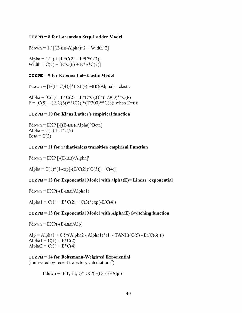
1 Biexponential Model 2 Density-weighted Biexponential Model 3 Off-set Gaussian with constant offset and E-dependent width 4 Biexponential Model with energy-dependent fraction 5 Generalized Gaussian with energy-dependent exponent 6 Generalized Gaussian plus Exponential term 7 Weibull Model 8 Lorentzian Step-Ladder Model 9 Exponential+Elastic Model 10 Klaus Luther's empirical function 11 Radiationless transition empirical function 12 Exponential Model with alpha(E)=linear + exponential 13 Exponential Model with alpha(E) switching function 14 Boltzmann-weighted exponential

39

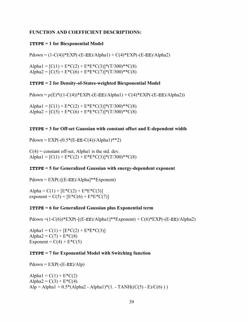
FUNCTION AND COEFFICIENT DESCRIPTIONS: ITYPE = 1 for Biexponential Model Pdown = (1-C(4))*EXP(-(E-EE)/Alpha1) + C(4)*EXP(-(E-EE)/Alpha2) Alpha1 = [C(1) + E*C(2) + E*E*C(3)]*(T/300)**C(8) Alpha2 = [C(5) + E*C(6) + E*E*C(7)]*(T/300)**C(8) ITYPE = 2 for Density-of-States-weighted Biexponential Model Pdown = r(E)*((1-C(4))*EXP(-(E-EE)/Alpha1) + C(4)*EXP(-(E-EE)/Alpha2)) Alpha1 = [C(1) + E*C(2) + E*E*C(3)]*(T/300)**C(8) Alpha2 = [C(5) + E*C(6) + E*E*C(7)]*(T/300)**C(8) ITYPE = 3 for Off-set Gaussian with constant offset and E-dependent width Pdown = EXP(-(0.5*(E-EE-C(4))/Alpha1)**2) C(4) = constant off-set, Alpha1 is the std. dev. Alpha1 = [C(1) + E*C(2) + E*E*C(3)]*(T/300)**C(8) ITYPE = 5 for Generalized Gaussian with energy-dependent exponent Pdown = EXP(-[(E-EE)/Alpha]**Exponent) Alpha = C(1) + [E*C(2) + E*E*C(3)] exponent = C(5) + [E*C(6) + E*E*C(7)] ITYPE = 6 for Generalized Gaussian plus Exponential term Pdown =(1-C(6))*EXP(-[(E-EE)/Alpha1]**Exponent) + C(6)*EXP(-(E-EE)/Alpha2) Alpha1 = C(1) + [E*C(2) + E*E*C(3)] Alpha2 = C(7) + E*C(8) Exponent = C(4) + E*C(5) ITYPE = 7 for Exponential Model with Switching function Pdown = EXP(-(E-EE)/Alp) Alpha1 = C(1) + E*C(2) Alpha2 = C(3) + E*C(4) Alp = Alpha1 + 0.5*(Alpha2 - Alpha1)*(1. - TANH((C(5) - E)/C(6) ) )

40

ITYPE = 8 for Lorentzian Step-Ladder Model Pdown = 1 / [(E-EE-Alpha)^2 + Width^2] Alpha = C(1) + [E*C(2) + E*E*C(3)] Width = C(5) + [E*C(6) + E*E*C(7)] ITYPE = 9 for Exponential+Elastic Model Pdown = [F/(F+C(4))]*EXP(-(E-EE)/Alpha) + elastic Alpha = [C(1) + E*C(2) + E*E*C(3)]*(T/300)**C(8) F = [C(5) + (E/C(6))**C(7)]*(T/300)**C(8); when E=EE ITYPE = 10 for Klaus Luther's empirical function Pdown = EXP [-[(E-EE)/Alpha]^Beta] Alpha = C(1) + E*C(2) Beta = C(3) ITYPE = 11 for radiationless transition empirical Function Pdown = EXP [-(E-EE)/Alpha]' Alpha = C(1)*[1-exp[-(E/C(2))^C(3)] + C(4)] ITYPE = 12 for Exponential Model with alpha(E)= Linear+exponential Pdown = EXP(-(E-EE)/Alpha1) Alpha1 = C(1) + E*C(2) + C(3)*exp(-E/C(4)) ITYPE = 13 for Exponential Model with Alpha(E) Switching function Pdown = EXP(-(E-EE)/Alp) Alp = Alpha1 + 0.5*(Alpha2 - Alpha1)*(1. - TANH((C(5) - E)/C(6) ) ) Alpha1 = C(1) + E*C(2) Alpha2 = C(3) + E*C(4)

ITYPE = 14 for Boltzmann-Weighted Exponential (motivated by recent trajectory calculations7)

Pdown = B(T;EE,E)*EXP( -(E-EE)/Alp )

41

B(T;EE,E) = SQRT(rho(EE)*exp(-(EE-E)/RT)) where rho(EE) = density of states Alp = C(1)

2.9 Format of External Data Files Location: EXTERNAL DATA FILES MUST BE STORED IN FOLDER

(DIRECTORY) "DensData", which is in the folder (directory) from which the MultiWell application is executed.

Densities, Sums and k(E)'s Creation: Typically, the external files for densities of states and sums of states are

generated using the program DenSum, which calculates sums and densities via exact counts. A similar format is used for specific rate constants, as described here.

FILE NAMES

For sums and densities of states: CHARACTER*10 + '.dens'

Example: 'Ethyl-Cl .dens' For specific rate constants [k(E)'s]: CHARACTER*10 + '.rke'

Example: 'HCl+C2H4.rke'

FILE FORMAT

Note: Starting with version 2008.1, " ____.dens" files, which contain sums and densities of states, may have a block of comment lines preceding Line 1 (below). The first and last comment lines in the block must have exactly the following 46 characters:

**************INPUT DATA SUMMARY**************

Line 1 (LINE COUNT IGNORES BLANK LINES FOLLOWING TITLE) Name of species or transition state [CHARACTER*10]: up to 10 characters (skipped when read by MultiWell, and therefore can be left blank) Line 2 Title/Comment line [CHARACTER*100]: up to 100 characters (skipped when read by MultiWell, and therefore can be left blank) Line 3 Egrain1 , imax1 , Emax2 , Isize , Viblo [REAL, INTEGER, REAL, INTEGER, REAL]

42

Note that this ordering of parameters is not the same as in multiwell.dat. If Egrain1, imax1, & Emax2 do not match those for the MultiWell run (see line #2 of the MultiWell data file), then execution terminates with a message. In density and sums of states files, Viblo is the lowest vibrational frequency for a given species; it is used in the collision step routines. In rate constant input files, A real number must be input for Viblo, but it is ignored by MultiWell. Line 4 Column labels (skipped when read by MultiWell, and therefore can be left blank) For sums of states, this line might read: " No. (cm-1) Density Sum"

For a rate constant input file, this line might read: " No. Energy Dummy RateConst" Line 5 (Repeated Isize times) j, A, B, C [INTEGER,REAL,REAL,REAL] FOR FILES CONTAINING SUMS & DENSITIES (these are double arrays) j = array element index (a total of Isize elements) A = energy starting with E = 0.0 (units: cm-1), which corresponds to the zero point energy of the

species or transition state. B = density of states (units: states/cm-1) C = sum of states (dimensionless) FOR FILES CONTAINING SPECIFIC RATE CONSTANTS [k(E)'s] (these are double arrays) j = array element index (a total of Isize elements) A = energy starting with E = 0.0 (units: cm-1). For reactions without tunneling, E=0 corresponds

to the zero point energy of the transition state (i.e. barrier height with zero point energy corrections), relative to the reactant energy (with zero point energy corrections). For reactions with tunneling, E = 0.0 corresponds to the lowest energy considered, which is usually significantly lower than the barrier height with zero point energy corrections (this same energy is entered in the MultiWell data file).

B = dummy real number (ignored by MultiWell) C = k(E) (units: s-1) Line 6 BLANK LINE TO INSURE THAT THE LAST LINE IS FOLLOWED BY A CARRIAGE RETURN (needed for all READ statements). THE CARRIAGE RETURN IS EASILY OVERLOOKED.

43

Initial Energy Distribution Function

File name: "multiwell.pstart" Location: EXTERNAL DATA FILES MUST BE STORED IN FOLDER (DIRECTORY) "DensData", which is in the folder (directory) from which the MultiWell application is executed. Line 1 (BLANK LINES ARE NOT ALLOWED) Jsize, Hstart, Edel

Jsize user-selected array length (≤14000 elements). Jsize must be chosen to be large

enough (for a given Hstart) so that the entire initial energy distribution is represented.

Hstart energy grain (express in cm-1) for initial energy distribution: "Pstart". Hstart should be ≥Egrain1 used to generate sums and densities of states.

Edel energy origin of array, relative to zero point energy of initial excited well (express in cm-1)

Line 2 (REPEAT Jsize times)

DUMMY, Pstart

DUMMY Must be input, but ignored by MultiWell (may be equal to E, for example) Pstart NORMALIZED cumulative initial energy distribution function. Thus,

Pstart(i) ranges monotonically from Pstart(1)=0 (approximately), up to Pstart(Jsize) = 1.0.

(Note that other columns may be present in the data file, but they will be ignored.)

Line 3 BLANK TO INSURE THAT THE LAST LINE IS FOLLOWED BY A CARRIAGE RETURN (needed for all READ statements). THE CARRIAGE RETURN IS EASILY OVERLOOKED.

44

2.10 Fatal Input Errors and Warnings

A FATAL INPUT ERROR is reported and execution is stopped if any of the following parameters for a well or transition state does not match the corresponding value from Line 2 of multiwell.dat:

Egrain1, imax1, Isize , Emax2

Incompatible Keywords or other Options, resulting in a Fatal Error: ILT and CENT1, CENT2, or CENTX ILT and TUN RKE and TUN CRP and TUN CENT and TUN CENT1, CENT2, or CENTX with TSmom(Mol,nchann) ≤ 0 (moment of inertia or rotational constant of the transition state)

Non-Fatal Warnings: "WARNING:numberofenergygrainswhereReactantWellhasstates,butProductWellhasnonetomatch[setk(E)=0]" This warning can arise when the density of states is sparse and some energy grains (“empty grains”) do not contain any ro-vibrational states. This can cause a problem when Well-to-Well reactions (especially tunneling reactions) are important. When reactions occur in MultiWell, population in an energy grain of the reactant Well passes to an energy grain of the product Well, but this process becomes undefined if the product energy grain does not contain any ro-vibrational states. This problem is most common when quantum mechanical tunneling is important, but it may also occur at energies above a reaction critical energy if the density of states in the product Well is particularly sparse. MultiWell handles this problem pragmatically by allowing the reaction to take place as long as the corresponding energy grain in the second Well not empty, and it forbids the reactiono and issues the Warning if the energy grain in the second Well is empty. This procedure is followed because states must be present in order to support population in any given energy grain, while standard barrier-tunneling models (like the Eckart model) implicitly assume that a continuum of (translational) states exists on both sides of the barrier. When the warning is issued, the user must decide whether the simulation is valid, since the “tunneling correction” is affected quantitatively when reactive flux is forbidden to pass into an empty grain. If tunneling is a very important component of the reaction model, then measures can be taken to minimize this problem (although the various measures may introduce other issues). Here are two ways to minimize this problem:

45

1. Larger energy grain sizes might be adopted, since with larger grain size there will be fewer empty energy grains. However, this measure will reduce the energy resolution, which is often (but not always) an important consideration. 2. When centrifugal corrections are being applied to a reaction (i.e. with keyword CENT2), densities of states are often sparse, because they are based only on the vibrations and the external K-rotor. Instead of using centrifugal corrections, one might instead use the Smith and Gilbert method of treating angular momentum17,19,23,24 (see Section A.2.3 in this User Manual). In this method, densities of states are computed based on the vibrations and ALL of the external rotational degrees of freedom, which significantly increases the density of states and greatly reduces the number of empty energy grains. This is a good approach when the Smith-Gilbert method is acceptable.

46

References

(1) Barker, J. R. Monte-Carlo Calculations on Unimolecular Reactions, Energy-Transfer, and

IR-Multiphoton Decomposition. Chem. Phys. 1983, 77, 301-318. (2) Barker, J. R. Radiative Recombination in the Electronic Ground State. J. Phys. Chem.

1992, 96, 7361-7367; DOI: 10.1021/j100197a042. (3) Barker, J. R. Multiple-well, multiple-path unimolecular reaction systems. I. MultiWell

computer program suite. Int. J. Chem. Kinet. 2001, 33, 232-245; https://doi.org/10.1002/kin.1017.



(6) Barker, J. R.; Ortiz, N. F. Multiple-Well, multiple-path unimolecular reaction systems. II. 2-methylhexyl free radicals. Int. J. Chem. Kinet. 2001, 33, 246–261; DOI: 10.1002/kin.1018.

(7) Barker, J. R.; Weston, R. E., Jr. Collisional Energy Transfer Probability Densities P(E,J;E',J') for Monatomics Colliding with Large Molecules. J. Phys. Chem. A 2010, 114, 10619–10633; 10.1021/jp106443d.

(8) Barker, J. R.; Yoder, L. M.; King, K. D. Feature Article: Vibrational Energy Transfer Modeling of Non-Equilibrium Polyatomic Reaction Systems. J. Phys. Chem. A 2001, 105, 796-809.

(9) Durant, J. L.; Kaufman, F. Calculation and use of total collision rates in thermal systems. CPL 1987, 142, 246-251.

(10) Forst, W. Unimolecular rate theory test in thermal reactions. J. Phys. Chem. 1972, 76, 342-348; https://doi.org/10.1021/j100647a012.

(11) Forst, W. Theory of Unimolecular Reactions; Academic Press: New York, 1973. (12) Forst, W. Unimolecular Reactions. A Concise Introduction; Cambridge University Press:

Cambridge, 2003. (13) Gillespie, D. T. A general method for numerically simulating the stochastic time

evolution of coupled chemical reactions. J. Comp. Phys. 1976, 22, 403-434. (14) Gillespie, D. T. Exact stochastic simulation of coupled chemical reactions. J. Phys.

Chem. 1977, 81, 2340-2361. (15) Gillespie, D. T. Monte Carlo simulation of random walks with residence time dependent

transition probability rates. J. Comp. Phys. 1978, 28, 395-407. (16) King, K. D.; Barker, J. R. Experiments on collisional energy transfer. In Unimolecular

Kinetics. Parts 2 and 3: Collisional Energy Transfer and The Master Equation; Robertson, S. H., Ed.; Elsevier, 2019; Vol. 43; pp 3-62.

(17) Klippenstein, S. J.; Harding, L. B. A direct transition state theory based study of methyl radical recombination kinetics. Journal of Physical Chemistry A 1999, 103, 9388-9398.

(18) Maranzana, A.; Barker, J. R.; Tonachini, G. Master Equation Simulations of Competing Unimolecular and Bimolecular Reactions: Application to OH Production in the Reaction

47

of Acetyl Radical with O2. Phys. Chem. Chem. Phys. 2007, 9, 4129 - 4141; DOI:10.1039/b705116f.


(20) Neufeld, P. D.; Janzen, A. R.; Aziz, R. A. Empirical Equations to Calculate 16 of the Transport Collision Integrals Ω(l, s)* for the Lennard‐Jones (12–6) Potential. J. Chem. Phys. 1972, 57, 1100.

(21) Olzmann, M. On the role of bimolecular reactions in chemical activation systems. Phys. Chem. Chem. Phys. 2002, 4, 3614–3618; https://doi.org/10.1039/B203244A.


(23) Smith, S. C.; Gilbert, R. G. Angular momentum conservation in multichannel unimolecular reactions. International Journal of Chemical Kinetics 1988, 20, 979-990.

(24) Smith, S. C.; Gilbert, R. G. Angular momentum conservation in unimolecular and recombination reactions. International Journal of Chemical Kinetics 1988, 20, 307-329.

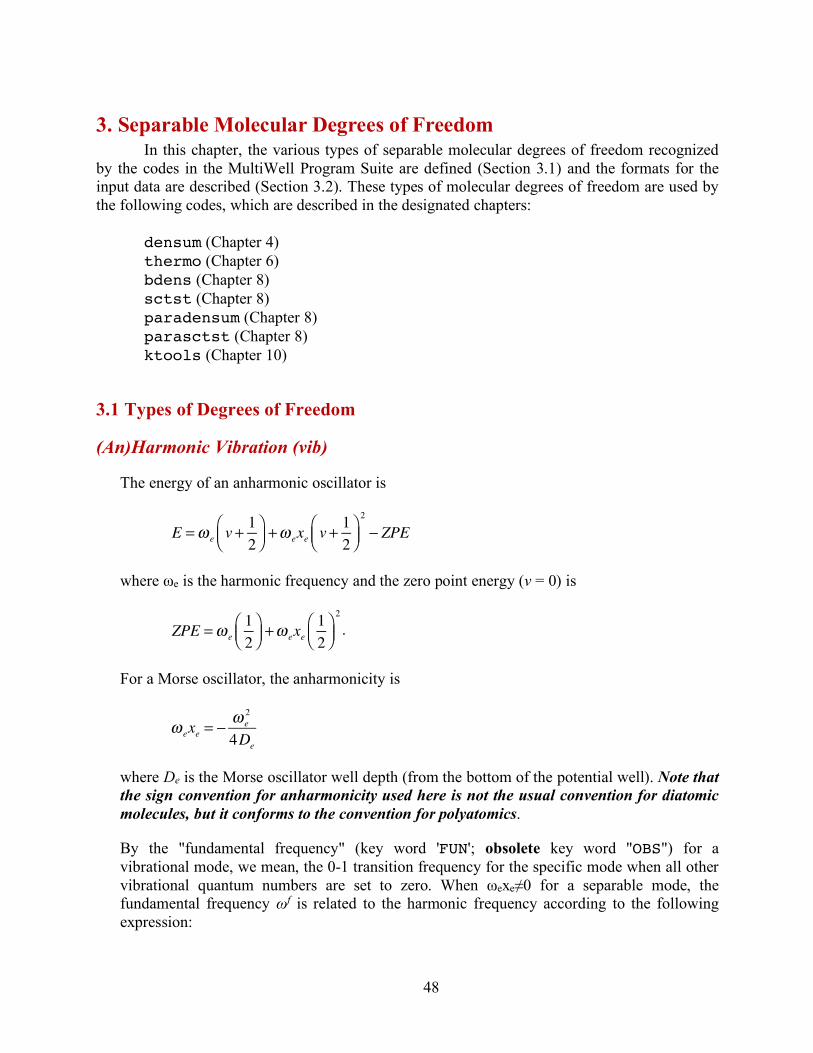
48

3. Separable Molecular Degrees of Freedom In this chapter, the various types of separable molecular degrees of freedom recognized

by the codes in the MultiWell Program Suite are defined (Section 3.1) and the formats for the input data are described (Section 3.2). These types of molecular degrees of freedom are used by the following codes, which are described in the designated chapters:

densum (Chapter 4) thermo (Chapter 6) bdens (Chapter 8) sctst (Chapter 8) paradensum (Chapter 8) parasctst (Chapter 8) ktools (Chapter 10)

3.1 Types of Degrees of Freedom

(An)Harmonic Vibration (vib)

The energy of an anharmonic oscillator is

where ωe is the harmonic frequency and the zero point energy (v = 0) is

.

For a Morse oscillator, the anharmonicity is

where De is the Morse oscillator well depth (from the bottom of the potential well). Note that the sign convention for anharmonicity used here is not the usual convention for diatomic molecules, but it conforms to the convention for polyatomics.

By the "fundamental frequency" (key word 'FUN'; obsolete key word "OBS") for a vibrational mode, we mean, the 0-1 transition frequency for the specific mode when all other vibrational quantum numbers are set to zero. When ωexe≠0 for a separable mode, the fundamental frequency ωf is related to the harmonic frequency according to the following expression:

E =ω e v + 12

⎛⎝⎜

⎞⎠⎟ +ω exe v + 1

2⎛⎝⎜

⎞⎠⎟2

− ZPE

ZPE =ω e12

⎛⎝⎜

⎞⎠⎟ +ω exe

12

⎛⎝⎜

⎞⎠⎟2

ω exe = − ω e2

4De

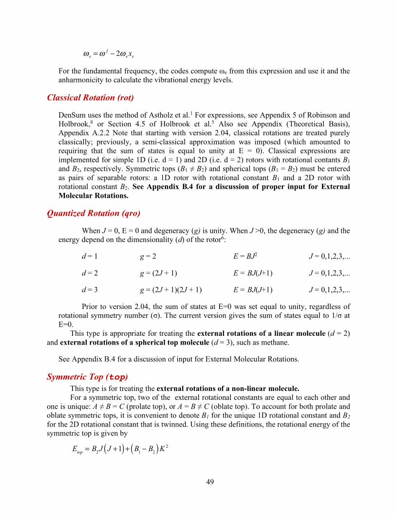
49

For the fundamental frequency, the codes compute ωe from this expression and use it and the anharmonicity to calculate the vibrational energy levels.

Classical Rotation (rot)

DenSum uses the method of Astholz et al.1 For expressions, see Appendix 5 of Robinson and Holbrook,8 or Section 4.5 of Holbrook et al.5 Also see Appendix (Theoretical Basis), Appendix A.2.2 Note that starting with version 2.04, classical rotations are treated purely classically; previously, a semi-classical approximation was imposed (which amounted to requiring that the sum of states is equal to unity at E = 0). Classical expressions are implemented for simple 1D (i.e. d = 1) and 2D (i.e. d = 2) rotors with rotational contants B1 and B2, respectively. Symmetric tops (B1 ≠ B2) and spherical tops (B1 = B2) must be entered as pairs of separable rotors: a 1D rotor with rotational constant B1 and a 2D rotor with rotational constant B2. See Appendix B.4 for a discussion of proper input for External Molecular Rotations.

Quantized Rotation (qro)

When J = 0, E = 0 and degeneracy (g) is unity. When J >0, the degeneracy (g) and the energy depend on the dimensionality (d) of the rotor6:

d = 1 g = 2 E = BJ2 J = 0,1,2,3,...

d = 2 g = (2J + 1) E = BJ(J+1) J = 0,1,2,3,...

d = 3 g = (2J + 1)(2J + 1) E = BJ(J+1) J = 0,1,2,3,...

Prior to version 2.04, the sum of states at E=0 was set equal to unity, regardless of rotational symmetry number (σ). The current version gives the sum of states equal to 1/σ at E=0.

This type is appropriate for treating the external rotations of a linear molecule (d = 2) and external rotations of a spherical top molecule (d = 3), such as methane.

See Appendix B.4 for a discussion of input for External Molecular Rotations.

Symmetric Top (top) This type is for treating the external rotations of a non-linear molecule. For a symmetric top, two of the external rotational constants are equal to each other and

one is unique: A ≠ B = C (prolate top), or A = B ≠ C (oblate top). To account for both prolate and oblate symmetric tops, it is convenient to denote B1 for the unique 1D rotational constant and B2 for the 2D rotational constant that is twinned. Using these definitions, the rotational energy of the symmetric top is given by

ω e =ωf − 2ω exe

Etop = B2J J +1( ) + B1 − B2( )K 2

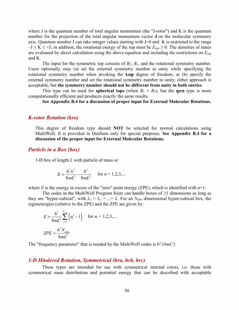
50

where J is the quantum number of total angular momentum (the "J-rotor") and K is the quantum number for the projection of the total angular momentum vector J on the molecular symmetry axis. Quantum number J can take integer values starting with J=0 and K is restricted to the range –J ≤ K ≤ +J; in addition, the rotational energy of the top must be Etop ≥ 0. The densities of states are evaluated by direct calculation using the above equation and including the restrictions on Etop and K.

The input for the symmetric top consists of B2, B1, and the rotational symmetry number. Users optionally may (a) set the external symmetry number to unity while specifying the rotational symmetry number when invoking the top degree of freedom, or (b) specify the external symmetry number and set the rotational symmetry number to unity; either approach is acceptable, but the symmetry number should not be different from unity in both entries.

This type can be used for spherical tops (when B1 = B2), but the qro type is more computationally efficient and produces exactly the same results.

See Appendix B.4 for a discussion of proper input for External Molecular Rotations.

K-rotor Rotation (kro)

This degree of freedom type should NOT be selected for normal calculations using MultiWell. It is provided in DenSum only for special purposes. See Appendix B.4 for a discussion of the proper input for External Molecular Rotations.

Particle in a Box (box)

1-D box of length L with particle of mass m:

for n = 1,2,3,...

where E is the energy in excess of the "zero" point energy (ZPE), which is identified with n=1. The codes in the MultiWell Program Suite can handle boxes of ≥1 dimensions as long as

they are "hyper-cubical", with Lx = Ly = ...= L. For an Ndim dimensional hyper-cubical box, the eigenenergies (relative to the ZPE) and the ZPE are given by:

for ni = 1,2,3,....

The "frequency parameter" that is needed by the MultiWell codes is h2/(8mL2).

1-D Hindered Rotation, Symmetrical (hra, hrb, hrc) These types are intended for use with symmetrical internal rotors, i.e. those with

symmetrical mass distribution and potential energy that can be described with acceptable

E = h2n2

8mL2− h2

8mL2

E = h2

8mL2 ni2 −1{ }

i=1

Ndim

∑

ZPE =

h2Ndim

8mL2

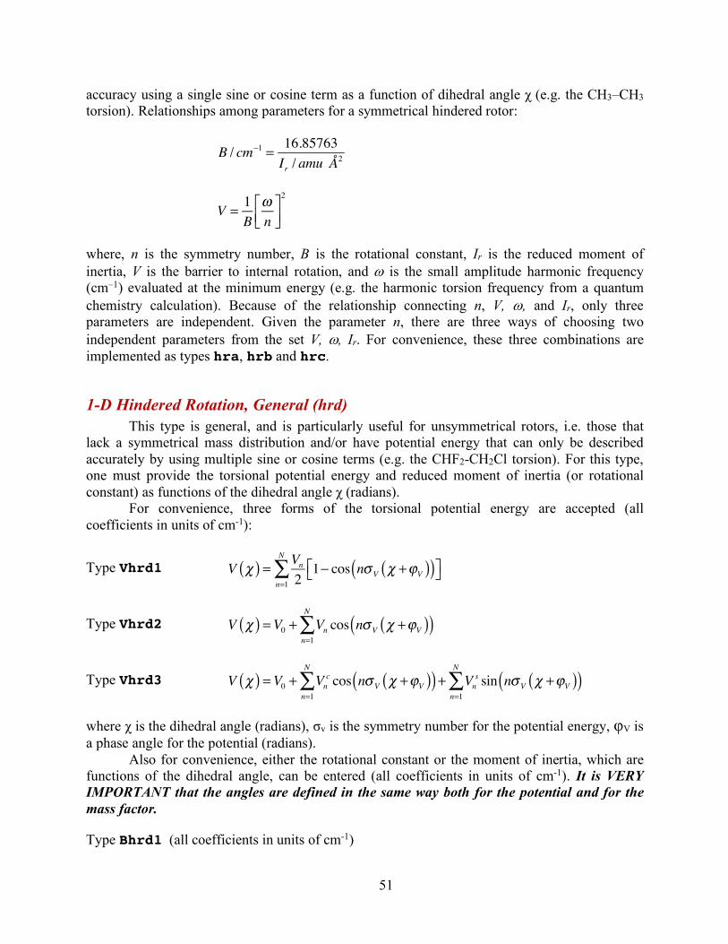
51

accuracy using a single sine or cosine term as a function of dihedral angle χ (e.g. the CH3–CH3 torsion). Relationships among parameters for a symmetrical hindered rotor:

where, n is the symmetry number, B is the rotational constant, Ir is the reduced moment of inertia, V is the barrier to internal rotation, and w is the small amplitude harmonic frequency (cm–1) evaluated at the minimum energy (e.g. the harmonic torsion frequency from a quantum chemistry calculation). Because of the relationship connecting n, V, w, and Ir, only three parameters are independent. Given the parameter n, there are three ways of choosing two independent parameters from the set V, w, Ir. For convenience, these three combinations are implemented as types hra, hrb and hrc.

1-D Hindered Rotation, General (hrd) This type is general, and is particularly useful for unsymmetrical rotors, i.e. those that

lack a symmetrical mass distribution and/or have potential energy that can only be described accurately by using multiple sine or cosine terms (e.g. the CHF2-CH2Cl torsion). For this type, one must provide the torsional potential energy and reduced moment of inertia (or rotational constant) as functions of the dihedral angle χ (radians).

For convenience, three forms of the torsional potential energy are accepted (all coefficients in units of cm-1):

Type Vhrd1

Type Vhrd2

Type Vhrd3

where χ is the dihedral angle (radians), σv is the symmetry number for the potential energy, φV is a phase angle for the potential (radians).

Also for convenience, either the rotational constant or the moment of inertia, which are functions of the dihedral angle, can be entered (all coefficients in units of cm-1). It is VERY IMPORTANT that the angles are defined in the same way both for the potential and for the mass factor.

Type Bhrd1 (all coefficients in units of cm-1)

B / cm−1 = 16.85763Ir / amu Å

2

V = 1B

ωn

⎡⎣⎢

⎤⎦⎥

2

V χ( ) = Vn21− cos nσV χ +ϕV( )( )⎡⎣ ⎤⎦

n=1

N

∑

V χ( ) =V0 + Vn cos nσV χ +ϕV( )( )n=1

N

∑

V χ( ) =V0 + Vnc cos nσV χ +ϕV( )( )

n=1

N

∑ + Vns sin nσV χ +ϕV( )( )

n=1

N

∑

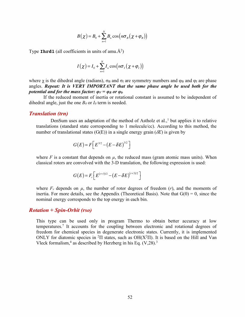
52

Type Ihrd1 (all coefficients in units of amu.Å2)

where χ is the dihedral angle (radians), σB and σI are symmetry numbers and φB and φI are phase angles. Repeat: It is VERY IMPORTANT that the same phase angle be used both for the potential and for the mass factor: φV = φB or φI.

If the reduced moment of inertia or rotational constant is assumed to be independent of dihedral angle, just the one B0 or I0 term is needed.

Translation (trn) DenSum uses an adaptation of the method of Astholz et al.,1 but applies it to relative

translations (standard state corresponding to 1 molecule/cc). According to this method, the number of translational states (G(E)) in a single energy grain (dE) is given by

where F is a constant that depends on µ, the reduced mass (gram atomic mass units). When classical rotors are convolved with the 3-D translation, the following expression is used:

where Fr depends on µ, the number of rotor degrees of freedom (r), and the moments of inertia. For more details, see the Appendix (Theoretical Basis). Note that G(0) = 0, since the nominal energy corresponds to the top energy in each bin.

Rotation + Spin-Orbit (rso)

This type can be used only in program Thermo to obtain better accuracy at low temperatures.7 It accounts for the coupling between electronic and rotational degrees of freedom for chemical species in degenerate electronic states. Currently, it is implemented ONLY for diatomic species in 2Π states, such as OH(X2Π). It is based on the Hill and Van Vleck formalism,4 as described by Herzberg in his Eq. (V,28).3

B χ( ) = B0 + Bn cos nσ B χ +ϕB( )( )n=1

N

∑

I χ( ) = I0 + In cos nσ I χ +ϕ I( )( )n=1

N

∑

G E( ) = F E 3/2 − E −δE( )3/2⎡⎣ ⎤⎦

G E( ) = Fr E r+3( )/2 − E −δE( ) r+3( )/2⎡⎣

⎤⎦

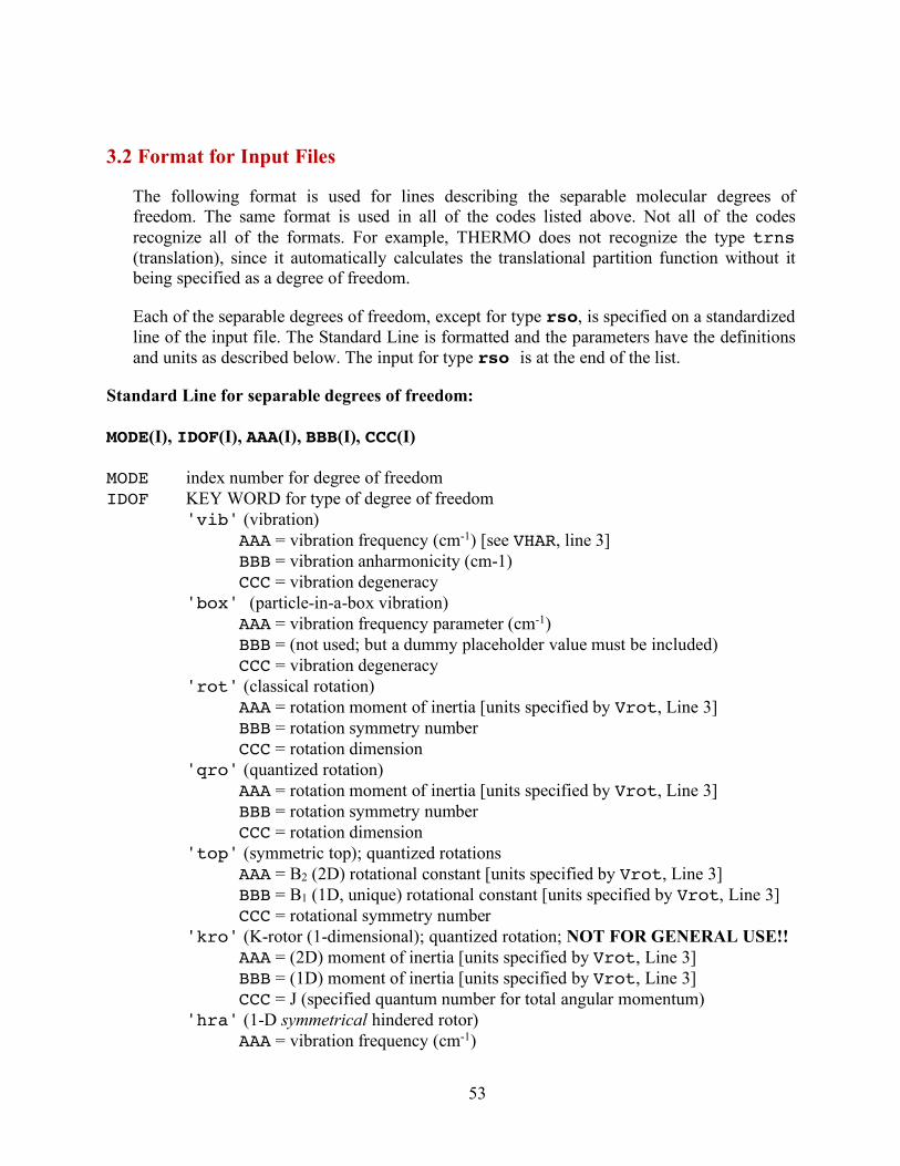
53

3.2 Format for Input Files

The following format is used for lines describing the separable molecular degrees of freedom. The same format is used in all of the codes listed above. Not all of the codes recognize all of the formats. For example, THERMO does not recognize the type trns (translation), since it automatically calculates the translational partition function without it being specified as a degree of freedom.

Each of the separable degrees of freedom, except for type rso, is specified on a standardized line of the input file. The Standard Line is formatted and the parameters have the definitions and units as described below. The input for type rso is at the end of the list.

Standard Line for separable degrees of freedom: MODE(I), IDOF(I), AAA(I), BBB(I), CCC(I)

MODE index number for degree of freedom IDOF KEY WORD for type of degree of freedom

'vib' (vibration) AAA = vibration frequency (cm-1) [see VHAR, line 3] BBB = vibration anharmonicity (cm-1) CCC = vibration degeneracy

'box' (particle-in-a-box vibration) AAA = vibration frequency parameter (cm-1) BBB = (not used; but a dummy placeholder value must be included) CCC = vibration degeneracy

'rot' (classical rotation) AAA = rotation moment of inertia [units specified by Vrot, Line 3] BBB = rotation symmetry number CCC = rotation dimension

'qro' (quantized rotation) AAA = rotation moment of inertia [units specified by Vrot, Line 3] BBB = rotation symmetry number CCC = rotation dimension

'top' (symmetric top); quantized rotations AAA = B2 (2D) rotational constant [units specified by Vrot, Line 3] BBB = B1 (1D, unique) rotational constant [units specified by Vrot, Line 3] CCC = rotational symmetry number

'kro' (K-rotor (1-dimensional); quantized rotation; NOT FOR GENERAL USE!! AAA = (2D) moment of inertia [units specified by Vrot, Line 3] BBB = (1D) moment of inertia [units specified by Vrot, Line 3] CCC = J (specified quantum number for total angular momentum)

'hra' (1-D symmetrical hindered rotor) AAA = vibration frequency (cm-1)

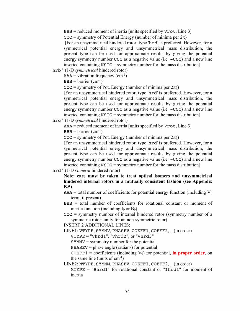
54

BBB = reduced moment of inertia [units specified by Vrot, Line 3] CCC = symmetry of Potential Energy (number of minima per 2p) [For an unsymmetrical hindered rotor, type 'hrd' is preferred. However, for a symmetrical potential energy and unsymmetrical mass distribution, the present type can be used for approximate results by giving the potential energy symmetry number CCC as a negative value (i.e. -CCC) and a new line inserted containing NSIG = symmetry number for the mass distribution]

'hrb' (1-D symmetrical hindered rotor) AAA = vibration frequency (cm-1) BBB = barrier (cm-1) CCC = symmetry of Pot. Energy (number of minima per 2p)) [For an unsymmetrical hindered rotor, type 'hrd' is preferred. However, for a symmetrical potential energy and unsymmetrical mass distribution, the present type can be used for approximate results by giving the potential energy symmetry number CCC as a negative value (i.e. -CCC) and a new line inserted containing NSIG = symmetry number for the mass distribution]

'hrc' (1-D symmetrical hindered rotor) AAA = reduced moment of inertia [units specified by Vrot, Line 3] BBB = barrier (cm-1) CCC = symmetry of Pot. Energy (number of minima per 2p)) [For an unsymmetrical hindered rotor, type 'hrd' is preferred. However, for a symmetrical potential energy and unsymmetrical mass distribution, the present type can be used for approximate results by giving the potential energy symmetry number CCC as a negative value (i.e. -CCC) and a new line inserted containing NSIG = symmetry number for the mass distribution]

'hrd' (1-D General hindered rotor) Note: care must be taken to treat optical isomers and unsymmetrical hindered internal rotors in a mutually consistent fashion (see Appendix B.5). AAA = total number of coefficients for potential energy function (including V0

term, if present). BBB = total number of coefficients for rotational constant or moment of

inertia function (including I0 or B0). CCC = symmetry number of internal hindered rotor (symmetry number of a

symmetric rotor; unity for an non-symmetric rotor) INSERT 2 ADDITIONAL LINES: LINE1: VTYPE, SYMMV, PHASEV, COEFF1, COEFF2, ...(in order) VTYPE = "Vhrd1", "Vhrd2", or "Vhrd3" SYMMV = symmetry number for the potential PHASEV = phase angle (radians) for potential COEFF1 = coefficients (including V0) for potential, in proper order, on

the same line (units of cm-1) LINE2: MTYPE, SYMMM, PHASEV, COEFF1, COEFF2, ...(in order) MTYPE = "Bhrd1" for rotational constant or "Ihrd1" for moment of

inertia

55

SYMMM = symmetry number for Bhrd1 or Ihrd1 PHASEM = phase angle (radians) for Bhrd1 or Ihrd1 COEFF1 = coefficients (including B0 or I0) for Bhrd1 (units of cm-1) or

Ihrd1 (amu•Å2 units), in proper order, on the same line 'trn' (3-dimensional relative translation)

AAA = mass of A (amu) BBB = mass of B (amu) CCC = ignored, but convenient to set it equal to "3"

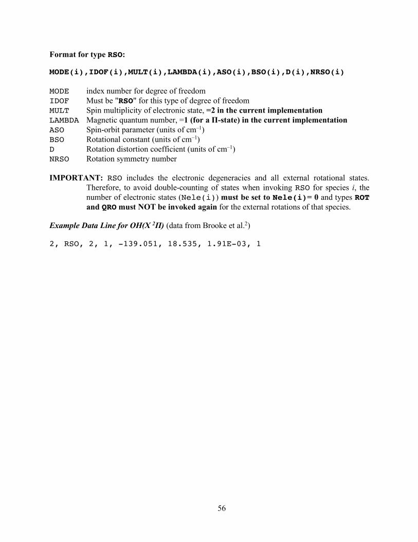
56

Format for type RSO:

MODE(i),IDOF(i),MULT(i),LAMBDA(i),ASO(i),BSO(i),D(i),NRSO(i) MODE index number for degree of freedom IDOF Must be "RSO" for this type of degree of freedom MULT Spin multiplicity of electronic state, =2 in the current implementation LAMBDA Magnetic quantum number, =1 (for a Π-state) in the current implementation ASO Spin-orbit parameter (units of cm–1) BSO Rotational constant (units of cm–1) D Rotation distortion coefficient (units of cm–1) NRSO Rotation symmetry number IMPORTANT: RSO includes the electronic degeneracies and all external rotational states.

Therefore, to avoid double-counting of states when invoking RSO for species i, the number of electronic states (Nele(i)) must be set to Nele(i)= 0 and types ROT and QRO must NOT be invoked again for the external rotations of that species.

Example Data Line for OH(X 2Π) (data from Brooke et al.2) 2, RSO, 2, 1, -139.051, 18.535, 1.91E-03, 1

57

References

(1) Astholz, D. C.; Troe, J.; Wieters, W. Unimolecular processes in vibrationally highly

excited cycloheptatrienes. I. Thermal isomerization in shock waves. J. Chem. Phys. 1979, 70, 5107-5116.

(2) Brooke, J. S. A.; Bernath, P. F.; Western, C. M.; Sneden, C.; Afşar, M.; Li, G.; Gordon, I. E. Line strengths of rovibrational and rotational transitions in the X2Π ground state of OH. J. Quant. Spectrosc. Radiat. Transf. 2016, 168, 142–157; http://dx.doi.org/10.1016/j.jqsrt.2015.07.021.

(3) Herzberg, G. Molecular Spectra and Molecular Structure. I. Spectra of Diatomic Molecules, 2 ed.; Van Nostrand Reinhold Co.: Cincinnati, 1950.

(4) Hill, E.; Van Vleck, J. H. On the Quantum Mechanics of the Rotational Distortion of Multiplets in Molecular Spectra. Phys. Rev. 1929, 32, 250-272.

(5) Holbrook, K. A.; Pilling, M. J.; Robertson, S. H. Unimolecular Reactions, 2 ed.; Wiley: Chichester, 1996.

(6) McHale, J. L. Molecular Spectroscopy; Prentice Hall: Upper Saddle River, 1999. (7) Nguyen, T. L.; Ruscic, B.; Stanton, J. F. A master equation simulation for the ÔH +

CH3OH reaction. J. Chem. Phys. 2019, 150, 084105; doi: 10.1063/1.5081827. (8) Robinson, P. J.; Holbrook, K. A. Unimolecular Reactions; Wiley-Interscience: London;

New York, 1972.

58

4. DenSum: Separable Sums and Densities of States This computer code carries out exact counts for sums and densities of states for separable

degrees of freedom via the Stein-Rabinovitch2 extension of the Beyer-Swinehart algorithm.1 Optionally, the Whitten-Rabinovitch approximation3,4 can be used.

Default array dimensions are easily changed in file src/densum/declare.inc

150 degrees of freedom (enough for a 50 atom molecule) 50000 energy grains (enough for 100000 cm-1 energy maximum, with 2 cm-1

grains) Output Files

densum.out File containing complete output. densum.lev Energy levels of quantized degrees of freedom. <FNAME>.dens File formatted for input into MultiWell.

Example data and output files are given in the examples directory: multiwell/examples/densum-examples.

4.1 DenSum Data File Format Note: Starting with version 2009.0, the data file format is no longer compatible with previous versions.

Line 1 TITLE (CHARACTER*180): up to 180 characters Line 2 FNAME

FNAME (CHARACTER*10): Filename to be created with ".dens" appended (up to 10

characters). Example: "hexadiene" produces file named "hexadiene.dens".

Line 3 N, IWR, VHAR,VROT

N no. of DoF's, IWR (flag) IWR 0: Uses exact state counts (energy grain = Egrain1) 1: Uses Whitten-Rabinovitch state densities VHAR KEYWORD for vibrations 'HAR': for vibrational frequencies input as harmonic frequencies. 'FUN': for vibrational frequencies input as 0-1 fundamental frequencies.

59

VROT KEYWORD for molecular internal and external rotations, except for hindered rotors of type hrd (see special instructions below for type hrd). Entries in upper or lower case:

'AMUA': for moments of inertia input with units of amu Å2. 'GMCM': for moments of inertia input with units of g cm2. 'CM-1': for rotational constant input with units of cm-1. 'MHZ': for rotational constant input with MHz. 'GHZ': for rotational constant input with GHz.

Notes: (a) All of the rotational information in a DenSum data file must be given in the form specified by VROT; (b) VHAR and VROT can be stated in either order on Line 3.

Line 4 Egrain1, Imax1, Isize, Emax2

Egrain1 energy grain in units of cm-1 Imax1 number of array elements in first segment of double array* Isize total size of double array (number of elements) Emax2 maximum energy (cm-1) for calculation

* Starting with MultiWell Version 2.08, densum.out provides information about the number of elements (Imax1) needed to achieve fluctuations of less than 5% in the density of states. If Egrain1 and Imax1 are chosen so that fluctuations in the density of states is greater than 5%, a warning is printed to the screen with a suggestion as to what Imax1 should be increased to. Note that a user can choose to disregard this warning and proceed to run MultiWell.

Line 5..N+3 MODE(I), IDOF(I), AAA(I), BBB(I), CCC(I)

MODE index number for degree of freedom IDOF KEY WORD for type of degree of freedom See Chapter 3 and for descriptions of the types of molecular degrees of freedom recognized by DENSUM.

Line N+4 BLANK LINE TO INSURE THAT THE LAST LINE IS FOLLOWED BY A CARRIAGE RETURN (needed for all READ statements). THE CARRIAGE RETURN IS EASILY OVERLOOKED.

60

4.2 DenSum in Batch Mode In order to run densum with the 'batch' option, one must first prepare a file:

densum.batch. This file lists the names of the DenSum data files (".vibs files") to be processed and the energy grain and double array boundaries. The batch file format is given below.

To use this option, the DenSum data files must all reside in one directory (e.g. directory

/vibs) and each must be named "<name>.vibs", where <name> does not contain any blank spaces. When listed in densum.batch, each file name must be listed on a separate line, including the extension ".vibs".

densum.batch Batch File Format

Line 1 Egrain1, Imax1, Isize, Emax2

Line 2 <name1>.vibs

Line 3 <name2>.vibs

Line 4 <name3>.vibs

.... etc.

<end of file> ------------------------------------- Sample densum.batch for three .vibs files

10. , 400 , 500 , 50000. B1.vibs B2.vibs CH3CO.vibs ------------------------------------

61

Execution

a) On linux:

From within the directory in which densum.batch and the .vibs data files reside,

type '<PATH>densum -batch' in a terminal shell, where PATH is the full path to the densum executable.

or

type 'densum -batch' in a terminal shell, if the PATH variable has been set to include the /bin directory that holds the densum executable.

or

type './densum -batch' in a terminal shell, if a copy of the densum executable resides in the same directory with densum.batch and the .vibs files.

b) On windows

There are two possibilities:

1) type "densum -batch" in a DOS shell

or

2) double-click on "densum-batch.bat". Note that densum.exe and densum-batch.bat must be in the same directory as densum.batch and the .vibs files.

62

References

(1) Beyer, T.; Swinehart, D. F. Number of multiply-restricted partitions. Comm. Assoc.

Comput. Machines 1973, 16, 379. (2) Stein, S. E.; Rabinovitch, B. S. Accurate evaluation of internal energy level sums and

densities including anharmonic oscillators and hindered rotors. J. Chem. Phys. 1973, 58, 2438-2445.

(3) Whitten, G. Z.; Rabinovitch, B. S. Accurate and Facile Approximation for Vibrational Energy‐Level Sums. J. Chem. Phys. 1963, 38, 2466.

(4) Whitten, G. Z.; Rabinovitch, B. S. Approximation for Rotation—Vibration Energy Level Sums. J. Chem. Phys. 1964, 41, 1883.

63

5. MomInert: Moments of Inertia This code was written mostly by Nicholas F. Ortiz under the direction of John R. Barker.

From Cartesian coordinates, it calculates the principal moments of inertia and approximate reduced moment of inertia for an internal rotation.

Example data and output files can be down-loaded from the MultiWell web site: http://aoss.engin.umich.edu/multiwell/.

Note that computer program lamm, described in Chapter 8 is designed to assist in computing moments of inertia as a function of dihedral angle. Thus lamm is more appropriate than MomInert for flexible internal rotations.

5.1 Data File Format Note: Starting with version 2.0, the data file format is no longer compatible with previous versions. To run Mominert using the default filename (mominert.dat):

LINUX/UNIX: in the directory where the input data file resides, type: <PATH>/multiwell-<version>/bin/mominert <RETURN>


~/multiwell-<version>/bin/mominert <RETURN> WINDOWS in a DOS window: in the directory where the input data file resides, type: <PATH>/multiwell-<version>/bin/mominert <RETURN> For example: ~/multiwell-2013/bin/mominert

To run Mominert using a user-defined filename (FileName.dat):

Follow the same procedures described above, but type: <PATH>/multiwell-<version>/bin/mominert <FileName> <RETURN>

For example: ~/multiwell-2013/bin/mominert final.dat The resulting output file will take the same prefix: final.out.

64

Line 1 TITLE A line, up to 100 characters, describing the data. This title is reproduced in the

output file. Line 2 UNITS Keyword designating units of coordinate values. ANGS Angstrom units. BOHR Atomic (Bohr) units (1 Bohr ≈ 0.529 Å) Line 3 NATOMS Total number of atoms in the molecule (up to 100 atoms). Line 4 (Repeat for every atom type [see Appendix B.7]) ATYPE, IA, X, Y, Z

ATYPE case sensitive atomic symbol, e.g. "C", "H", "Br79" (see Sec. 9.7) IA Index number of the atom (1 to NATOMS). X,Y,Z Cartesian coordinates (Å or Bohr; see Line 2) of the atom. To assign an arbitrary mass to an atom:

1. Designate "XX" for ATYPE (instead of e.g. "H" or "C") in Line 3. 2. On the line following the atom type designation, insert a line giving the mass to be

assigned to this particular atom. This must be done each time a special mass is to be assigned. It is not necessary for the mass to always be the same. In other words, atom type "XX" may be designated multiple times in the same molecule, and a different mass may be specified each time.

Line 5 IAI, IAJ Atom indices for the two atoms defining the axis of internal rotation. If the atom indices are set equal to zero, then internal rotor is not calculated and Line 6 and Line 7 can be omitted. Line 6 NR

65

Number of atoms in one of the two rotating moieties. Line 7 List of the atom indices that comprise the rotating moiety containing NR atoms. Line 8 For additional internal rotors, REPEAT lines 5-7. TO TERMINATE, enter two zeros: "0 , 0". Line 9 BLANK LINE TO INSURE THAT THE LAST LINE IS FOLLOWED BY A CARRIAGE RETURN (needed for all READ statements). THE CARRIAGE RETURN IS EASILY OVERLOOKED.

5.2 Computational Approach This code uses the two axis-defining atoms and one other atom to define two

perpendicular planes which intersect at the rotation axis. The distance from all atoms in the molecule to each plane is calculated. The Pythagorean Theorem is then used to define the distance of each atom to the axis. The mass is defined for each atom type, and then the mass and distance are used to calculate the moment of inertia for the internal rotations in amu Å2.

The center-of-mass is then defined. This is used to calculate all external products and moments of inertia. These values are put into the proper matrix, and eigenvalues are found. The eigenvalues are the principle moments of inertia.

For the reduced moment of inertia for internal rotation, MomInert uses the approximation that the reduced moment is calculated for the axis that contains the twisting bond. This approximation is reasonably accurate (errors of less than 5-10%) for many species.1

References

(1) East, A. L. L.; Radom, L. Ab initio statistical thermodynamical models for the computation of third-law entropies. J. Chem. Phys. 1997, 106, 6655-6673.

66

6. thermo: Thermodynamics

6.1 Introduction

thermo calculates equilibrium constants, thermodynamic parameters, and canonical transition state theory (CTST) rate constants (including Eckart tunneling through an unsymmetrical barrier) via standard statistical mechanics formulae. It can also compute canonical rate constants using W. H. Miller's Semiclassical Transition State Theory (SCTST) when used in conjunction with programs sctst and bdens, or paradensum.

Example data and output files are given in the examples directory Note that the data file for Thermo (thermo.dat) is intentionally very similar in

format to the data file for DenSum (densum.dat). Thus major parts of the data files can be copied and pasted.

6.1.1 Thermodynamic Output When given a collection of molecular properties, thermo uses statistical mechanics

formulae to calculate the corresponding thermodynamics parameters. Thermo can also calculate canonical transition state theory rate constants. The input and output are intended to be easily understood, but some items are explained below.

Three output files are generated by THERMO. "thermo.out" is the general output file,

which contains all of the information needed by most users. The following two output files are useful, but of less general interest. "thermo.details" displays contributions from every degree of freedom to the heat capacity, entropy, and enthalpy function for each chemical species at 298.15 K and groupings of degrees of freedom at each temperature. "thermo.partfxns" displays the partition functions for grouped degrees of freedom for each chemical species at each temperature. (The grouped degrees of freedom include electronic, translational, vibrational, free rotational, and hindered rotational.)

Standard State: the standard state must be selected. The conventional standard state for most data tabulations is 1 bar, ideal gas. For analysis involving reaction rate constants, it is usually appropriate to choose the standard state of 1 molecule cm-3. The units and numerical values of entropies, equilibrium constants and other thermodynamic quantities are determined by the selection of the standard state.

Standard States recognized by THERMO: • 1 bar, ideal gas (keyword BAR) • 1 atm, ideal gas (keyword ATM) • 1 molecule cm-3, ideal gas (keyword MCC) • free translations ignored (keyword NOT)

67

Molar Enthalpy: The enthalpy for formation at 0 K is required input. THERMO output echoes the input and also reports the enthalpy of formation at 298.15 K and the standard free energy of formation (DelG(298)).

For convenience, THERMO recognizes several energy units for enthalpy, which can be selected by the user:

• kJ/mol (keyword KJOU) • kcal/mol (keyword KCAL) • cm-1 (wavenumbers) (keyword CM-1)

Equilibrium constant: Note that the numerical value of the equilibrium constant depends on the standard state. Kequil is reported for each temperature listed in the input file. The values of Kequil generally fall on a curved line when plotted on an Arrhenius plot (log (Kequil) vs. 1/T): Kequil = A(T)*exp(B(T)/T). The parameters A(T) and B(T)are based on the local slope: d(ln Keq)/d(1/T). This slope is evaluated by finite differences centered on each T and the results are usually accurate to within 1%, or better, at the specified T. The error is mostly due to round-off error in the value of Arrhenius parameter B. For best accuracy, one should use THERMO to evaluate Kequil at each and every temperature of interest.

Canonical Transition State Theory Rate Constant (CTST): Note that the user must select the standard state of 1 molecule cm-3 (i.e. "MCC") when calculating rate constants. Rate constant "k(T)" is reported for each temperature listed in the input file. In addition, it is reported as the Arrhenius function of temperature: k(T) = A(T)*exp(B(T)/T). The parameters A(T) and B(T)are based on the local slope: d(ln (k(T)))/d(1/T). This slope is evaluated by finite differences centered on each T and the results are usually accurate to within 1%, or better, at the specified T. The error is mostly due to round-off error in the value of Arrhenius parameter B. For best accuracy, one should use THERMO to evaluate k(T) at each and every temperature of interest.

Molar Entropy: the numerical value for the entropy depends on the standard state that is selected, as well as on the enthalpy units that are selected.

Molar Heat Capacity: Cp depends on enthalpy units that are selected.

Enthalpy Function: [H(T)-H(0)] depends on the enthalpy units that are selected.

Accuracy: All accuracies depend on the accuracy of the input data. For a given set of input data, the

accuracies achieved by THERMO are relative to a benchmark based on the same input data. The benchmarks most commonly used are taken from the NIST-JANAF Thermochemical Tables.1 Note that when rotations are treated classically, the entropy, heat capacity, free energy, and equilibrium constant are less accurate at low temperatures.

• molecular weights are accurate to 0.002 g mol-1, or better.

68

• enthalpies and Gibbs free energy for individual species generally agree with the JANAF tables to within 0.05 kJ mol-1, or better.

• entropies computed for individual species are generally accurate to 0.1 J K-1 mol-1 or better.

• electronic partition function is accurate to 0.1% or better.

• enthalpy, entropy, heat capacity, and Gibbs free energy differences for reaction (DelS(rxn), DelH(rxn), DelCp(rxn) and DelG(rxn), respectively) are generally more accurate than the corresponding quantities for the individual species, due to cancellation of errors.

6.1.2 Types of Degrees of Freedom

The following types used by THERMO are described in Chapter 3: Harmonic or Anharmonic Vibration (vib) Classical Rotation (rot) Quantized Rotation (qro) Symmetric Top (top): Particle in a Box (box) 1-D Hindered Rotation, Symmetrical (hra, hrb, hrc) 1-D Hindered Rotation, General (hrd)

The following types are unique to THERMO:

Hindered Gorin Model (gor) and Fitting (fit) Thermo includes the capability to automatically find the hindrance parameters for the

Hindered Gorin transition state.2-7,10,11 One can choose one or both of the following types (IDOF) of degrees of freedom.

1) IDOF = gor selected for one vibrational stretching mode. For a selected potential energy function, Thermo finds the center of mass distance rmax corresponding to maximum of Veffective at temperature T, where the rotational energy in the 2-D pseudo-diatomic rotation is assumed to be RT. From the value of rmax, Thermo computes the 2-D moment of inertia.

2) IDOF = fit selected for two (linear molecule) or three (non-linear) rotational dimensions. Thermo finds the hindrance parameters γ (gamma) and η (eta) that produce a good fit at each temperature to experimental rate constants (one for each temperature) that are entered.

γ = 1−η( )1/2

69

If both IDOF = gor and IDOF = fit are selected, Thermo finds the maximum of Veffective and uses it to find the hindrance parameters (gamma and eta) that produce a good fit to experimental rate constants (one for each of the Nt temperatures) that are entered.

The selectable potential energy functions are:

MORSE (Morse Oscillator)

VARSHNI (Varshni Oscillator12)

sMORSE ("Stiff Morse" Oscillator)

This is a Morse oscillator, but replaces with ; cs is

an empirical parameter and must be ≥0.

The input is assumed to correspond to the following generic recombination reaction:

In the thermo input, A and B are labeled as reactants ("reac") and C‡ is labeled as a transition state ("ctst"). For a barrier-less recombination reaction, the enthalpy of formation at 0 K (DelH) for C‡ must be set equal to the sum of the enthalpies of formation for the two reactants. All of the internal and rotational degrees of freedom for A and B are entered as usual. The internal degrees of freedom for C‡ consist of the combined degrees of freedom (internal and external) of A and B, plus the external rotations for C‡. Thus the number of degrees of freedom (including degeneracies and multiple dimensions) of C‡ is

where nA and nB are the total number of degrees of freedom for A and B, and nCrots is the number of external rotations of C‡.

VMorse r( ) = De 1− exp −βMorse r − re( )⎡⎣ ⎤⎦{ }2 − De

βMorse = 2πνeµ2De

VVarshni (r) = De 1−rer

⎛⎝⎜

⎞⎠⎟ exp −βVarshni r

2 − re2( )⎡⎣ ⎤⎦

⎧⎨⎩

⎫⎬⎭

2

− De

βVarshni =12re

2πν µ2De

− 1re

⎡

⎣⎢

⎤

⎦⎥ =

12re

βMorse −1re

⎡

⎣⎢

⎤

⎦⎥

βMorse βStiff = βMorse 1+ cs r − re( )2⎡⎣

⎤⎦

A + B→C‡

nC = nA + nB + nCrots

70

In order to find the center of mass distance rmax corresponding to maximum of Veffective at temperature T, the external 2-D rotation for C‡ is labeled "gor" (see below). This signals that this particular entry is a dummy and will be adjusted in the process of finding the maximum Veffective. The potential energy function is specified later in the data file (see below).

In order to adjust the "hindrance" to fit specified rate constants, some of the rotations in C‡ that were originally associated with A and B must be multiplied by γ (see above). These are labeled "fit" (see below). These rotations do not include internal rotation about the new bond in C‡, but only the rotations about internal axes perpendicular to the new bond. Later in the data file, the (experimental) rate constants to be fitted are entered... one for each temperature.

Fully Coupled Anharmonic Vibrations (qvb)

This type specifies that program Thermo must read a supplementary data file named <name>.qvib, generated by programs bdens (Section 8.1), or paradensum (Section 8.2). This supplementary file must be present in the same directory as data file thermo.dat.

By using this supplementary data file, Thermo can utilize full intermode vibrational anharmonic coupling when computing thermodynamic data. This coupling is most important at high temperatures. This option is used when computing thermal rate constants with semi-classical transition state theory (SCTST; see Sections 8.3 and B.9 for more details).

IMPORTANT NOTE: Programs bdens and paradensum can optionally include separable degrees of freedom of the types listed in Chapter 3. In this case, the supplementary file <name>.qvib includes these degrees of freedom as well. To avoid double-counting, any separable degrees of freedom included in the bdens or paradensum calculations should not be listed again in the thermo data file.

Thermal Rate Constants from SCTST (crp)

This type specifies that program Thermo reads a supplementary data file named <name>.qcrp, which must be generated previously by program sctst (Section 8.3) or parsctst (Section 8.4). File <name>.qcrp must be present in the same directory as data file thermo.dat. See Sections 8.3, 8.4, and B.9 for more details. By using this supplementary data file, Thermo can utilize the semi-classical transition state theory (SCTST) of W. H. Miller and coworkers. SCTST accounts for fully coupled degrees of freedom, including the reaction coordinate. As a result, the theory incorporates multidimensional quantum tunneling along the curved reaction path, which is very important at low temperatures. To prevent applying a second tunneling correction, the imaginary frequency, vimag, (entered on Line 5, see below) must be given a value of vimag = 0.0 (actually <20 cm-1), or execution of THERMO will be terminated.

Note that in order to obtain the best possible accuracy at both low and high temperatures, a fully coupled vibrational model for a unimolecular reactant is usually used in addition to the crp degree of freedom when computing SCTST rate constants. The fully coupled vibrational model is specified with degree of freedom type "qvb" (see above) and it requires a supplementary data file from program bdens, or paradensum (see Chapter 8).

IMPORTANT NOTE: Programs parsctst and sctst can optionally include separable degrees of freedom of the types listed in Chapter 3. In this case, the supplementary file

71

<name>.qcrp includes these degrees of freedom as well. To avoid double-counting, any separable degrees of freedom included in the parsctst and sctst calculations should not be listed again in the thermo data file.

Rotation Coupled to Spin-Orbit Splitting (rso)

This type accounts for the coupling between electronic and rotational degrees of freedom for chemical species in degenerate electronic states. Currently, it is implemented ONLY for diatomic species in 2Π states, such as OH(X2Π). It is based on the Hill and Van Vleck formalism,9 as described by Herzberg in his Eq. (V,28).8 It is invoked in order to obtain better accuracy at low temperatures.

72

6.2 Data File Format Note: Starting with version 2009.0, the data file format is no longer

compatible with previous versions. To run Thermo using the default filename (thermo.dat):

LINUX/UNIX: in the directory where the input data file resides, type: <PATH>/multiwell-<version>/bin/thermo <RETURN>


~/multiwell-<version>/bin/thermo <RETURN> WINDOWS in a DOS window: in the directory where the input data file resides, type: <PATH>/multiwell-<version>/bin/thermo <RETURN> For example: ~/multiwell-2013/bin/thermo

To run Thermo using a user-defined filename (FileName.dat):

Follow the same procedures described above, but type: <PATH>/multiwell-<version>/bin/thermo <FileName> <RETURN>

For example: ~/multiwell-2013/bin/thermo final.dat The resulting output file will take the same prefix: final.out.

Line 1 EKEY , SSKEY

EKEY Key Word for Enthalpy units: "KCAL" or "KJOU" (upper or lower case). Note that "CM-1" is a reserved keyword to be fully implemented later.

SSKEY Key Word for Standard State: "BAR", "ATM", "MCC" (molecule/cc), or "NOT" (free translations ignored)

73

Line 2 Nt number of temperatures Line 3 T1, T2, T3,... List of Nt temperatures Line 4 Ns number of chemical species Line 5 for reactants, products, or "none"; see below for transition states REPROD, MOLNAME, DelH REPROD key word: "reac" = reactant "prod" = product "none" = not included in equilibrium constant MOLNAME Name of chemical species (up to 32 characters) DelH enthalpy of formation at 0 K (Note that absolute enthalpies are not necessary, as

long as the enthalpy differences between reactants and products are correct.) Line 5' for transition states REPROD, MOLNAME, DelH, vimag, VVR REPROD = "ctst" For transition states, only. This choice calculates the canonical transition state

theory rate constant based on reactant and transition state parameters. It assumes the reaction consists of reactants (each labeled "reac") and a transition state (labeled "ctst"). Note that for bimolecular and termolecular reactions, the standard state should be set to "MCC" for concentration units.

For 1-D quantum mechanical tunneling via an unsymmetrical Eckart energy barrier, enter vimag >0 and VVR >0. Eckart tunneling is neglected when vimag <20 cm-1 and/or VVR = 0.0.

For use with SCTST rate constants, vimag = 0.0 and/or VVR must be set equal to 0.0 in order to prevent including tunneling twice (i.e. once via the SCTST rate constants and again via 1-D Eckart tunneling) vimag = 0.0 and/or VVR = 0.0

MOLNAME Name of transition state (up to 32 characters) DelH enthalpy of formation at 0 K. (Note that absolute enthalpies are not necessary, as

long as the enthalpy differences between reactants and transition state are correct.)

74

vimag magnitude of imaginary frequency (units of cm-1). When using "crp" files from program sctst (see section 8.3), vimag must set to 0.0 cm-1.

VVR Height of barrier for the reverse reaction (energy units specified in Line 1). When using crp files from program sctst (see section 8.3), VVR must be set to 0.0, but must be entered. Eckart tunneling is neglected when VVR = 0.0.

Line 6 FORMULA Empirical chemical formula written in the usual way with atomic symbols. These

symbols include "D" for deuterium and "T" for tritium. Special atomic symbols used for other isotopic species (e.g. "Cl35") are summarized in Section 10.7. Whenever an atomic symbol includes numeric characters (e.g. "Cl35"), it must be enclosed in square brackets, e.g. "[Cl35]". Examples of empirical formulas: C2H6O, CH3CH2OH, (CH3)2OH, (CH3)2(N)O2H, CH[Br79]2(CH3)3, CH3OD, C([C13]H3)4.

Line 7 Up to 20 comment lines. The first non-blank character on each comment line must be "!" (omit the quotation marks). Line 8 Sym, Sopt, Nele Sym external symmetry number (INTEGER); see Appendices B.4 and B.5 Sopt number of optical isomers (INTEGER); see Appendix B.5 Nele number of electronic energy levels (INTEGER) NOTE: Nele ≥ 1, except Nele = 0 (required!) when invoking IDOF(i) = 'RSO'

type for the coupled electronic-rotation degrees of freedom in 2∏ diatomics (like OH radical).

Line 9

Elev, gele (Repeat line for Nele electronic states)

Elev electronic level energies (REAL), always expressed as wavenumbers (cm–1). NOTE: lowest energy level should be at energy Elev = 0.0. gele electronic level degeneracies (INTEGER)

Line 10

N , VHAR , VROT number of vibrations and rotations to be read in

VHAR KEYWORD for vibrations

75

'HAR': for vibrational frequencies input as harmonic frequencies. 'FUN': for vibrational frequencies input as 0-1 fundamental frequencies. VROT KEYWORD for molecular internal and external rotations, except for hindered rotors

of type hrd (see special instructions below for type hrd). Entries in upper or lower case:

'AMUA': for moments of inertia input with units of amu Å2. 'GMCM': for moments of inertia input with units of g cm2. 'CM-1': for rotational constant input with units of cm-1. 'MHZ': for rotational constant input with MHz. 'GHZ': for rotational constant input with GHz.

Note: All of the rotational information for a given molecular species must be given in the form specified by VROT for that species.

Line 11

(repeat N times for the N molecular degrees of freedom)

MODE(I), IDOF(I), AAA(I), BBB(I), CCC(I) MODE index number for degree of freedom IDOF KEY WORD for type of degree of freedom See Section 6.1.2 and Chapter 3 for descriptions of the types of separable molecular degrees of freedom recognized by THERMO.

RETURN TO LINE #5 and REPEAT FOR THE NEXT CHEMICAL SPECIES AFTER ALL CHEMICAL SPECIES HAVE BEEN ENTERED, RESUME HERE:

Line 12 (when 'fit' is used) kexp(1), kexp(2), .... list of Nt experimental recombination rate constants (units of cm3 molecule-1 s-1): one for each of the Nt temperatures.

Line 13-17 (required if 'gor' is used) Line 13 readpot Keyword 'MORSE', 'VARSHNI', or 'sMORSE' (Stiff-Morse).

This is the type of bonding potential energy function. Line 14 freq Harmonic frequency (cm-1) of the normal mode associated with the

forming bond. Line 15 De Dissociation Energy De (units of Eunit) of the forming bond. Line 16 re EQUILIBRIUM center-of-mass distance (Å) between the of the two

fragments that are forming the new bond. Line 17 c Stiff-Morse parameter (needed only for 'sMORSE' type of potential).

Line 18 (BLANK LINE)

76

6.3 MultiWell Thermodynamics Database A database of molecular constants (for use by program thermo) is provided on the

MultiWell website. The chemical species in this database are of interest to us in our research. We add entries from time to time, depending on current research interests.

The following are some excellent sources of molecular constants and enthalpies, which can be used with program thermo to generate thermodynamics data:

• NIST WebBook [http://webbook.nist.gov/chemistry/] • Active Thermochemical Tables [http://atct.anl.gov/] • NIST Computational Chemistry Comparison and Benchmark Database (NIST Standard

Reference Database Number 101 Release 18, October 2016, Editor: Russell D. Johnson III) [http://cccbdb.nist.gov/]

• NIST-JANAF Thermochemical Tables.1

References

(1) Chase, M. W., Jr. NIST-JANAF Thermochemical Tables. Fourth Edition. J. Phys. Chem.

Ref. Data 1998, Monograph No. 9, 1-1951. (2) Golden, D. M. Reaction ClO+ClO--> Products: Modeling and Paremeterization for Use

in Atmospheric Models. International Journal of Chemical Kinetics 2003, 35, 206-211. (3) Golden, D. M. Evaluating data for atmospheric models, an example:

CH3O2+NO2=CH3O2NO2. International Journal of Chemical Kinetics 2005, 37, 625-632.

(4) Golden, D. M. Evaluating data for atmospheric models, an example: IO+NO2=IONO2. Journal of Physical Chemistry A 2006, 110, 2940-2943.

(5) Golden, D. M. The reaction Cl+NO2 -> ClONO and ClNO2. Journal of Physical Chemistry A 2007, 111, 6772-6780.

(6) Golden, D. M.; Barker, J. R.; Lohr, L. L. Master Equation Models for the Pressure- and Temperature-Dependent Reactions HO + NO2 -> HONO2 and HO + NO2 -> HOONO. JPCA 2003, 107, 11057-11071.

(7) Golden, D. M.; Smith, G. P. Reaction of OH + NO2 + M: A new view. JPCA 2000, 104, 3991-3997.

(8) Herzberg, G. Molecular Spectra and Molecular Structure. I. Spectra of Diatomic Molecules, 2 ed.; Van Nostrand Reinhold Co.: Cincinnati, 1950.

(9) Hill, E.; Van Vleck, J. H. On the Quantum Mechanics of the Rotational Distortion of Multiplets in Molecular Spectra. Phys. Rev. 1929, 32, 250-272.

(10) Patrick, R.; Golden, D. M. Int. J. Chem. Kinet. 1983, 15, 1189-1227. (11) Smith, G. P.; Golden, D. M. Application of RRKM Theory to Reactions OH+NO2+N2 =

HONO2+N2 (1) and ClO+NO2+N2 = ClONO2+N2 (2) - Modified Gorin Model Transition-State. IJCK 1978, 10, 489.

77

(12) Varshni, Y. P. Comparative Study of Potential Energy Functions for Diatomic Molecules. Rev. Mod. Phys. 1957, 29, 664-682.

78

7. gauss2multi: A Tool for Creating Data Files

In many cases, one wants to create data files from calculated properties of molecules and transition states. The program gauss2multi is a tool designed to assist in this process. The source code is located in the multiwell/src directory and the executable is located in the multiwell/bin directory. The tool reads vibrational frequencies, coordinates, and energies from the standard .log or .out output files produced by GAUSSIAN 982 and GAUSSIAN 03.1

This tool does not create complete data files: it inserts only the data produced by quantum chemistry codes. It inserts some additional information as placeholders: the user must review the files created by gauss2multi and insert missing data and replace the placeholder data. We recommend that new users create input files manually, so that they will become familiar with the required input data. Experienced users will gain more benefit when using gauss2multi. In order to convert GAUSSIAN output files into multiwell input files you need:

• GAUSSIAN output files with frequency calculation (file extension: .log or .out) • gauss2multi.cfg configuration file, which must reside in the same directory as the

gaussian output files. An example is found in the examples directory The following files will be created for each GAUSSIAN file that is read: FILE NAME DESCRIPTION (see MultiWell User Manual)

name.coords | mominert input file name.coords.out | mominert output file name.vibs | densum input file name.dens | densum output file name.therm| | thermo input file name.therm.out | thermo output file multiwell.dat | rough drat fof multiwell input file ("name" refers to the GAUSSIAN file name, which cannot exceed 10 characters in length)

gauss2multi.cfg Configuration File

You can create and edit the configuration file by yourself or use the step-by-step script to create it. The gauss2multi.cfg configuration file contains the following items (an example file is given below):

Line:

1. Energy units: KCAL , KJOU, or CM-1 (upper or lower case) 2. number of temperatures

79

3. list of temperatures separated by one or more blank spaces 4. Pressure units: TOR, BAR, ATM, or MCC (upper or lower case). [Note: the TOR

pressure unit is not one of the allowed standard states, which are required for setting up data file thermo.dat; therefore, BAR is used as default in creating thermo.dat.]

5. number of pressures 6. list of pressures separated by one or more blank spaces 7. Egrain, imax1, Isize, Emax2 8. index number (ascending order), name of gaussian output file (.log or .out), type

of structure: WELL, PROD, or TS (upper or lower case) 9. Repeat Line-8 for additional species.

TO RUN gauss2multi There are two modes of operation: (a) To set up files for an entire multi-species model.

In this case, the energies (i.e. ∆Hf0(0 K)) for all of the species will be calculated with respect to the energy of the first well (index number = 1) listed in gauss2multi.cfg. In the same directory as the GAUSSIAN files, type 'gauss2multi'

or (b) To generate data files for a single species.

In the same directory as the GAUSSIAN files, type 'gauss2multi <GAUSSIAN _Name_File>'

IMPORTANT:

The conversion to MultiWell data files cannot be completely automated: Many of these files will require manual changes! Be careful!

EXAMPLE CONFIGURATION FILE (gauss2multi.cfg) KCAL 3 298.15 398 498 TOR 5 0.1 1.0 10. 100. 1000. 10. 400 900 50000. 1 A.log WELL 2 B.log WELL 3 TS-A-B.log TS 4 C.log PROD

80

References

(1) Frisch, M. J.; Trucks, G. W.; Schlegel, H. B.; Scuseria, G. E.; Robb, M. A.; Cheeseman,

J. R.; Montgomery, J. A., Jr.; Vreven, T.; Kudin, K. N.; Burant, J. C.; Millam, J. M.; Iyengar, S. S.; Tomasi, J.; Barone, V.; Mennucci, B.; Cossi, M.; Scalmani, G.; Rega, N.; Petersson, G. A.; Nakatsuji, H.; Hada, M.; Ehara, M.; Toyota, K.; Fukuda, R.; Hasegawa, J.; Ishida, M.; Nakajima, T.; Honda, Y.; Kitao, O.; Nakai, H.; Klene, M.; Li, X.; Knox, J. E.; Hratchian, H. P.; Cross, J. B.; Bakken, V.; Adamo, C.; Jaramillo, J.; Gomperts, R.; Stratmann, R. E.; Yazyev, O.; Austin, A. J.; Cammi, R.; Pomelli, C.; Ochterski, J. W.; Ayala, P. Y.; Morokuma, K.; Voth, G. A.; Salvador, P.; Dannenberg, J. J.; Zakrzewski, V. G.; Dapprich, S.; Daniels, A. D.; Strain, M. C.; Farkas, O.; Malick, D. K.; Rabuck, A. D.; Raghavachari, K.; Foresman, J. B.; Ortiz, J. V.; Cui, Q.; Baboul, A. G.; Clifford, S.; Cioslowski, J.; Stefanov, B. B.; Liu, G.; Liashenko, A.; Piskorz, P.; Komaromi, I.; Martin, R. L.; Fox, D. J.; Keith, T.; Al-Laham, M. A.; Peng, C. Y.; Nanayakkara, A.; Challacombe, M.; Gill, P. M. W.; Johnson, B.; Chen, W.; Wong, M. W.; Gonzalez, C.; Pople, J. A. Gaussian 03, Revision C.02; Gaussian, Inc.: Wallingford CT, 2004.

(2) Frisch, M. J.; Trucks, G. W.; Schlegel, H. B.; Scuseria, G. E.; Robb, M. A.; Cheeseman, J. R.; Zakrzewski, V. G.; Montgomery, J.; Stratmann, R. E.; Burant, J. C.; Dapprich, S.; Millam, J. M.; Daniels, A. D.; Kudin, K. N.; Strain, M. C.; Farkas, O.; Tomasi, J.; Barone, V.; Cossi, M.; Cammi, R.; Mennucci, B.; Pomelli, C.; Adamo, C.; Clifford, S.; Ochterski, J.; Petersson, G. A.; Ayala, P. Y.; Cui, Q.; Morokuma, K.; Malick, D. K.; Rabuck, A. D.; Raghavachari, K.; Foresman, J. B.; Cioslowski, J.; Ortiz, J. V.; Baboul, A. G.; Stefanov, B. B.; Liu, G.; Liashenko, A.; Piskorz, P.; Komaromi, I.; Gomperts, R.; Martin, R. L.; Fox, D. J.; Keith, T.; Al-Laham, M. A.; Peng, C. Y.; Nanayakkara, A.; Challacombe, M.; Gill, P. M. W.; Johnson, B.; Chen, W.; Wong, M. W.; Andres, J. L.; González, C.; Head-Gordon, M.; Replogle, E. S.; Pople, J. A. Gaussian 98, Revision A.7 Pittsburgh, 1998.

81

82

8. bdens, paradensum, parsctst, and sctst: non-Separable Vibrations

Program bdens computes sums and densities of states for non-separable vibrations. In addition to fully-coupled non-separable vibrations, the code can also include separable degrees of freedom, such as free rotations and hindered internal rotations. The code combines two fundamentally different algorithms:

a) Brute force direct counting (via a recursive algorithm), which is suitable for both small and large molecules at energies low enough so that the total sum of states is not too large. For some small molecules, direct brute force counting can be carried out even at energies above the dissociation energy.

b) The Wang-Landau algorithm, which his most suitable for large molecules at high energies.4,14,21

Direct counting produces exact sums and densities of states, but it is very slow when the total sum of states is large. The Wang-Landau algorithm is computationally quite efficient, but suffers from stochastic fluctuations unless a very large number of stochastic samples is used. In addition, its sampling is impeded when the density of states is very sparse. In program bdens, the two algorithms are combined in one "smart" code that produces exact (directly counted) results at low energies, where the density of states is sparse, and rapidly computed results of sufficient accuracy at high energies, where the densities and sums of states are very large.

Program paradensum is a parallelized, improved version replacing adensum, which is no longer supported (its last release was in multiwell-2014.1b). paradensum computes sums and densities of states for fully-coupled vibrational models. It utilizes the Wang-Landau algorithm with a flatness criterion and is suitable for fully-coupled vibrational models that consist of from 3 to >100 degrees of freedom.

The third program, parsctst, is for computing rate constants by using semi-classical transition state theory (SCTST) of W. H. Miller and coworkers, as described below. It is a parallelized, improved that will replace the serial code sctst in a future release. At the user's option, parsctst can be executed either as a serial code, or as a parallel code, thus effectively replacing the older code sctst.

Anharmonic vibrations For a brief introduction to non-separable anharmonic vibrations and definitions of

technical terms, see Technical Note #2 (Appendix B.2 of this User Manual). Note that "exact" refers to exact at the level of second order vibrational perturbation theory (VPT2).

NOTE. In VPT2, the zero point energy includes contributions from the harmonic frequencies, the anharmonicities, and an additional term denoted G0 (see Eq. 9 in Appendix B.9).13,19 This term, which cancels-out in spectroscopy applications but must be included for thermochemistry and kinetics, is computed by electronic structure programs that employ VPT2 (e.g. GAUSSIAN and CFOUR), but it is not computed by MultiWell. For ab initio kinetics calculations involving small molecules the term may be significant, but it is very small for molecules with small rotational constants. For high accuracy ab initio kinetics calculations (e.g. 16, G0 can be included manually by modifying the reaction critical energy (E0).

83

Acceptable Vibrational States The vibrational energy Ev in principle can be computed when all acceptable values of v

are known. Acceptable values of v correspond to bound vibrational states. Therefore, the problem reduces to finding all acceptable values of v up to a given total internal energy. For a separable harmonic oscillator, all quantum numbers from v=0 to v=∞ are acceptable. A Morse oscillator, however, can dissociate and thus has a finite number of acceptable vibrational states ranging from v=0 to v=vmax. For a coupled set of anharmonic vibrations, the maximum quantum number allowed for the kth vibration, vD,k, depends on the quantum numbers assigned for all other vibrations; the dissociation energy of the kth vibration corresponds to the energy at which Ev reaches a maximum as uk is increased, i.e. (∂Ev/∂vk) = 0 at vk = vD,k.3,14,16 For a state to be "bound" with respect to the kth degree of freedom, the derivative must be greater than zero for the trial value of quantum number vk: (∂Eu/∂vk)>0. In the codes bdens, paradensum, and parsctst, this criterion must be satisfied for a quantum number to be deemed "acceptable". In addition, quantum numbers in parctst must also satisfy the condition that the amplitude of the effective imaginary frequency (which is affected by coupling to all of the other vibrations) must be greater than zero.

G0 Term in the ZPE from VPT2 In second order vibrational perturbation theory (VPT2), the zero point energy includes

contributions from the harmonic frequencies, the anharmonicities, and an additional term denoted G0 (see Eq. 9 in Appendix B.9).13,19 This term, which cancels-out in spectroscopy applications but must be included for thermochemistry and kinetics, is computed by electronic structure programs that employ VPT2 (e.g. GUSSIAN and CFOUR), but it is not computed by MultiWell. For ab initio kinetics calculations involving small molecules the term may be significant, but it is very small for molecules with small rotational constants. For high accuracy ab initio kinetics calculations (e.g. 16, G0 can be included manually by modifying the reaction critical energy.

8.1 Program bdens Program bdens replaces previous programs adensum, doloops, and ansum, which

were last released in version 2014.1b. For definitions of the terms used in the following, see Technical Note #2 (Appendix B.2 of this User Manual).

Program bdens computes sums and densities of acceptable bound and quasi-bound states as a function of vibrational energy Ev up to a high energy (measured from the zero point energy). The state energies are binned in energy grains specified by user (typically 10 cm-1). Total sums and densities of states can then be computed by convoluting the results for the fully coupled vibrational model with separable degrees of freedom, such as rotations, hindered rotors, etc. (using the combined Beyer-Swinhart5 and Stein-Rabinovitch18 algorithms (the BSSR algorithm)).

Program bdens combines two algorithms: direct count and the Wang-Landau algorithm. The resulting sums and densities of states are exact at low energies (where direct counting is used) and of very high accuracy at high energies (where the Wang-Landau) method is used. For

84

larger species, the combination gives both faster execution times and better accuracy at low energies.

Direct count Algorithm The direct count (DC) algorithm is a recursive version of a set of nested do-loops.

Because it is recursive, it (ideally) can be used for any number of coupled vibrational modes; practically speaking, the default array size limits the number of vibrations to 150, which is large enough for most applications.

Wang-Landau Algorithm Wang and Landau20,21 pioneered an efficient random walk algorithm in energy space to

compute densities of states for use in classical statistical models. Their approach is based on the idea that a density-weighted Monte Carlo sampling of the energy states of the system will produce a flat histogram of samples in equally-spaced energy bins if the density of states function is exact, in the limit of an infinite number of trials. The algorithm is initiated with a trial density of states in every energy bin and the density-weighted Monte Carlo sampling begins. A histogram records every visit to an energy bin. The algorithm is designed to modify the relative density of states G(Ei) on every visit to an energy bin (at energy Ei) in such a way so that G(Ei) approaches exact proportionality with the true density of states after a large number of samples.20,21 The algorithm can be halted by monitoring the "flatness" of the histogram, or by limiting the number of Monte Carlo samples. Basire et al.4 adapted the Wang-Landau algorithm for computing quantum densities of states for fully coupled anharmonic systems using the perturbation theory expansion for vibrational energy. It is a powerful method. For a full description of the algorithm and notation, see the paper by Basire et al. 4 As one of their demonstrations, they computed the density of states for naphthalene, based on the fully-coupled X matrix reported by Cané et al.6

We have modified the Basire et al. version4 of the Wang-Landau algorithm in several minor ways to meet the needs for the density of states in chemical kinetics and master equation applications. In our approach, we compute statistics for the histogram based only on energy bins that contain states. We do not use the "flatness" criterion for halting the algorithm, but instead use the number of Monte Carlo trials per energy bin, since that is the principal factor that controls the relative error (see below). We also apply the tests described above to ensure that selected states are bound or quasi-bound.

We have automated the algorithm by choosing the probability of accepting a move (parameter p; see Basire et al. for notation) according to N, the number of DOF. As discussed by Basire et al., if p is too large, the Monte Carlo selection can sample the entire energy range rapidly, but there may be many wasted samples that fall out of range. On the other hand if p is too small, the entire energy range may not be sampled efficiently, and more trials will be needed. In this work, we adopt p =MIN(1/N, 0.25). This protocol is consistent with the values for p used by Basire et al.4 As discussed in a later section, our results show little sensitivity to the selection of p.

An important new modification we have made to the Basire et al. version4 of the Wang-landau algorithm is to introduce automatic normalization of the density of states. Recall that the Wang-Landau algorithm produces results that are proportional to the exact density of states. The un-normalized G(Ei) may be sufficient for many applications, but the absolute density of states ρ(Ei) is needed for calculating rate constants from statistical rate theories, for example. In our

85

approach, the size of the energy bins (i.e. the energy grain size ∆E) is chosen small enough so that only one state, the lowest energy state (i.e. the zero point energy state), falls in the lowest energy bin. Since we know that only one state resides in the lowest energy bin, the density of states in lowest energy bin must be (∆E)-1, we then obtain the absolute density of states:

For vibrational states, it is easy to choose ∆E small enough so that only the zero point energy state falls within the lowest energy bin.

In the bdens code, this normalization method has been improved by taking advantage of the exact state count obtained from the Direct Count algorithm. The DC algorithm is used to calculate exact densities of states in an energy range that overlaps the energy range in which the WL algorithm is used. The overlapped energy range is approximately from Eswitch to 1.1*Eswitch. Over that overlapped energy range, the ratio of the exact density of states divided by the relative density of states is evaluated in each occupied energy grain and the average is identified with the scale factor that normalizes the WL relative densities. Since this scale factor depends on not just one, but on multiple energy grains, it is not as susceptible to stochastic noise as our original normalization method.

Note that our modified version14 of the Wang-Landau algorithm20,21 draws heavily on that of Basire et al., 4 which should also be cited.

Switching from Direct Count to Wang-Landau At energy Eswitch, the bdens code switches execution from the direct count (DC)

algorithm to the Wang-Landau (WL) algorithm (see next section). Eswitch can be optionally declared manually (by choosing keyword "MAN " and giving the energy Eswitch (cm–1 units)) or automatically (keyword "AUTO"). By carrying out tests, we have determined how the execution time using each algorithm depends on the sum of states as a function of energy. At low energies, DC is faster than the WL, while the reverse is true at high energies. When Eswitch is determined automatically, it is selected in order to minimize total execution time. In other words, the "AUTO" option results nearly optimum over-all execution times.

Running bdens The executable (binary) program resides in the directory

multiwell<version>/bin, where <version> is the version number (e.g. "2010.0") To execute the compiled program, enter the directory that contains the bdens data file ("bdens.dat") and then type ~/multiwell<version>/bin/ bdens. Directory multiwell<version> is assumed to reside in your Home directory. The output file bdens.out is automatically placed in the directory that contains bdens.dat. A second output file <name>.dens, which is designed to be an input file for the MultiWell master equation code, is also generated, where <name> is the name of the chemical species (specified in bdens.dat).

bdens has been designed to run using a "checkpoint file" (<name>.chk), which is generated after the density of states of the fully coupled vibrations have been calculated; this is the most time-consuming section. The following section convolutes the separable degrees of

ρ Ei( ) = G Ei( )

G Ei = 0( )1ΔE

86

freedom, if any are specified. The separable degrees of freedom may include free or hindered rotors, harmonic vibrations, etc. In particular, the K-rotor and possibly other external rotational degrees of freedom may be specified. If desired, the densities of states may be recalculated using various combinations of separable degrees of freedom, but retaining the same set of fully coupled vibrations. Repetitive calculations like these can be restarted using the checkpoint file, which saves considerable computer time.

In addition to the checkpoint file (<name>.chk), three output files are generated by bdens: bdens.out, <name>.dens, and <name>.qvib. The first file (bdens.out) is a standard output file, which summarizes all input and output. The second file (<name>.dens), which takes a chemical species name (<name>) as part of the file name, gives sums and densities of states, formatted as double arrays; it can be used as input for the MultiWell master equation code. By using this input file, master equation calculations can be carried out with densities of states computed by including the fully-coupled vibrations. The third file (<name>.qvib) is formatted as a supplementary input file for program Thermo; it tabulates the partition function and other thermodynamic properties of the coupled vibrational modes at a set of fixed temperatures from 50 K to >3000 K. Thermo can utilize these partition functions to compute and thermodynamics data and canonical rate constants. See Section 6.3 of this User Manual for a description of how the <name>.qvib file is used by Thermo.

bdens.dat Data File Format

For definitions of terms, see Technical Note #9. (Appendix B.2 of this User Manual)

Line 1: Name (species name; ≤10 characters)

Line 2: Title 1 (≤100 characters)

Line 3: Title 2 (≤100 characters) Line 4: ns (number of vibrational modes), NY (number of Y matrix elements), NZ (number of Z matrix elements), WW (a keyword to designate frequencies as ωe or ω0) WW = We for ω WW = Wf for fundamental vibrations (0-1 transitions) WW = W0 for ω0 [note: "0" is a zero]

(The distinction between ω and ω0 is explained by eqs. (II,267) through (II,269) of Herzberg 8. The computer code carries out the conversion between them.)

Lines 5+ (5 to 4+ns): wa(i) [i = 1 , ns] vibrational frequencies (cm-1)

Line 6 (5+ns): KEYWORD for reading the X anharmonicity matrix: = lower (for reading lower half of matrix, plus the diagonal) = upper (for reading upper half of matrix, plus the diagonal)

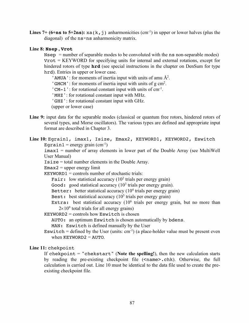
87

Lines 7+ (6+ns to 5+2ns): xa(k,j) anharmonicities (cm-1) in upper or lower halves (plus the diagonal) of the ns×ns anharmonicity matrix.

Line 8: Nsep , Vrot Nsep = number of separable modes to be convoluted with the ns non-separable modes) Vrot = KEYWORD for specifying units for internal and external rotations, except for hindered rotors of type hrd (see special instructions in the chapter on DenSum for type hrd). Entries in upper or lower case.

'AMUA': for moments of inertia input with units of amu Å2. 'GMCM': for moments of inertia input with units of g cm2. 'CM-1': for rotational constant input with units of cm-1. 'MHZ': for rotational constant input with MHz. 'GHZ': for rotational constant input with GHz. (upper or lower case)

Line 9: input data for the separable modes (classical or quantum free rotors, hindered rotors of several types, and Morse oscillators). The various types are defined and appropriate input format are described in Chapter 3.

Line 10: Egrain1, imax1, Isize, Emax2, KEYWORD1, KEYWORD2, Eswitch Egrain1 = energy grain (cm-1) imax1 = number of array elements in lower part of the Double Array (see MultiWell User Manual) Isize = total number elements in the Double Array. Emax2 = upper energy limit KEYWORD1 = controls number of stochastic trials:

Fair: low statistical accuracy (102 trials per energy grain) Good: good statistical accuracy (103 trials per energy grain). Better: better statistical accuracy (104 trials per energy grain) Best: best statistical accuracy (105 trials per energy grain) Extra: best statistical accuracy (106 trials per energy grain, but no more than

2´109 total trials for all energy grains) KEYWORD2 = controls how Eswitch is chosen

AUTO: an optimum Eswitch is chosen automatically by bdens. MAN: Eswitch is defined manually by the User

Eswitch = defined by the User (units: cm-1) (a place-holder value must be present even when KEYWORD2 = AUTO.

Line 11: chekpoint If chekpoint = "chekstart" (Note the spelling!), then the new calculation starts by reading the pre-existing checkpoint file (<name>.chk). Otherwise, the full calculation is carried out. Line 10 must be identical to the data file used to create the pre-existing checkpoint file.

88

Notes

1. Energies are relative to the zero point energy. 2. Be careful when using Gaussian! The Gaussian log file has two sections related to

vibrations. The first section is for the usual vibrational analysis to obtain harmonic frequencies. These frequencies are listed from lowest to highest. The second section is for anharmonicities. In the second section, the harmonic frequencies are listed again (along with the fundamental frequencies), but the ordering may not be the same as in the first section. The input for the codes distributed in MultiWell will accept the frequencies in any order, but the ordering of the harmonic frequencies must be consistent with the ordering used for the anharmonicities. For consistency, the Gaussian user must be sure to use the ordering of the harmonic frequencies as listed in association with the anharmonicities in the Gaussian log file.

89

8.2 Program paradensum

paradensum:1 parallel and improved version of adensum (adensum was last released in multiwell-2014.1b)

Program Authors: paradensum: C. Aieta, F. Gabas, and M. Ceotto adensum: T. L. Nguyen and J. R. Barker

Contact: Michele Ceotto: [email protected] (For definitions, see Technical Note #2. (Appendix B.2 of this User Manual)) Wang and Landau20,21 pioneered an efficient random walk algorithm in energy space to

compute densities of states for use in classical statistical models. Their approach is based on the idea that a density-weighted Monte Carlo sampling of the energy states of the system will produce a flat histogram of samples in equally-spaced energy bins if the density of states function is exact, in the limit of an infinite number of trials. The algorithm is initiated with a trial density of states in every energy bin and the density-weighted Monte Carlo sampling begins. A histogram records every visit to an energy bin. The algorithm is designed to modify the relative density of states G(Ei) on every visit to an energy bin (at energy Ei) in such a way so that G(Ei) approaches exact proportionality with the true density of states after a large number of samples.20,21 The algorithm can be halted by monitoring the "flatness" of the histogram, or by limiting the number of Monte Carlo samples. Basire et al.4 adapted the Wang-Landau algorithm for computing quantum densities of states for fully coupled anharmonic systems using the perturbation theory expansion for vibrational energy. It is a powerful method. For a full description of the algorithm and notation, see the paper by Basire et al. 4 As one of their demonstrations, they computed the density of states for naphthalene, based on the fully-coupled X matrix reported by Cané et al.6

We have modified the Basire et al. version4 of the Wang-Landau algorithm in several minor ways to meet the needs for the density of states in chemical kinetics and master equation applications.14 In our approach, we compute statistics for the histogram based only on energy bins that contain states. In paradensum we use the “flatness” criterion for halting the algorithm (this is in contrast to adensum, which used specified numbers of stochastic trials). We also apply the tests described elsewhere3 to ensure that selected states are bound or quasi-bound.

We have automated the algorithm by choosing the probability of accepting a move (parameter p; see Basire et al. for notation) according to N, the number of coupled DOF.14 As discussed by Basire et al., if p is too large, the Monte Carlo selection can sample the entire energy range rapidly, but there may be many wasted samples that fall out of range. On the other hand if p is too small, the entire energy range may not be sampled efficiently, and more trials will be needed. In this work, we adopt p =MIN(1/N, 0.25). This protocol is consistent with the values for p used by Basire et al.4 Our results show little sensitivity to the selection of p.

The most important new modification we have made to the Basire et al. version4 of the Wang-landau algorithm is to introduce automatic normalization of the density of states.1,14 Recall that the Wang-Landau algorithm produces results that are proportional to the exact density of states. The un-normalized G(Ei) may be sufficient for many applications, but the absolute density

90

of states ρ(Ei) is needed for calculating partition functions and rate constants from statistical rate theories, for example. In our approach, the size of the energy bins (i.e. the energy grain size ∆E) is chosen small enough so that only one state, the lowest energy state (i.e. the zero point energy state), falls in the lowest energy bin. Since we know that only one state resides in the lowest energy bin, the density of states in lowest energy bin must be ρ(0) = 1/∆E, we then obtain the absolute density of states:

For vibrational states, it is easy to choose ∆E small enough so that only the zero point energy state falls within the lowest energy bin. For master equation and chemical kinetics applications, the typical energy grain is ∆E≤10 cm-1 and vibrational frequencies are typically much larger. If rotations were to be included with the vibrations, normalization can still be achieved easily by using one of the other methods described above to count the number of rotational states in the lowest energy grain and normalizing accordingly.

Our modified version of the Wang-Landau algorithm20,21 draws heavily on that of Basire et al., 4 and is summarized elsewhere.1,14 Also see Section 8.1 of this User Manual for a description of program bdens, which also uses the Wang-Landau algorithm.

paradensum is a parallel code that can exploit not only single but also multiple core architectures. In this way the computation of the density of states is significantly accelerated when considering high dimensionality systems. The parallelization strategy is to divide the energy range into energy “windows” and set the calculations of G(Ei) for each window on a single processor. This strategy is dictated by the observation that less random sampling events and reduced computational effort is needed for Monte Carlo to converge in a restricted energy range.

The number of processors is given by the windowing choice and, by default, all windows have the same width. This setting can be changed modifying the appropriate keyword in the input file. If the computational time spent by each window to reach the flatness criterion is unbalanced, the code prints a warning in the Windows_info.txt output file. Then, the user can decide to halve the width of the first two or the last two windows.

Since the Wang-Landau density of states is notoriously biased at the edges of small energy windows, we always keep a percentage of overlap between neighbor windows. This is also necessary for the normalization of the G(Ei) obtained in each window to give the complete function on the whole energy domain.1 The code supports the possibility to run serially multiple walkers in each energy window. This feature improves the statistics of sampling in each window but does not have any impact on the speedup. To run the code the user has to supply the number of processors that is equal to the number of windows and a percentage of overlap between them as input parameters. When the number of processors (windows) is set to unity, then paradensum will run in serial mode (i.e. it can run on a single cpu or core). The set up of the input file for these parameters is described below. For a full description of the paradensum implementation, see the paper by Aieta et al.1

Running paradensum paradensum is a parallel code. To compile and run the code, it is necessary to have

previously installed supplementary software. Details are given in Section 1.4). paradensum has been designed to run using a "checkpoint file" (<name>.chk),

which is generated after the density of states of the fully coupled vibrations have been calculated,

91

which is the most time-consuming section. The next section in the code convolutes the separable degrees of freedom, if any are specified. The separable degrees of freedom may optionally include free or hindered rotors, harmonic vibrations, etc. In particular, the K-rotor and possibly other external rotational degrees of freedom may be specified. If desired, the densities of states may be recalculated using various combinations of separable degrees of freedom, but retaining the same set of fully coupled vibrations, available from the checkpoint file. Repetitive calculations like these can be restarted using the checkpoint file, which saves considerable computer time. Note that when using checkpoint file, it is not necessary to run the code in parallel mode.

The input data file paradensum.dat includes molecular parameters for computing the densities of states, as well as parallel execution parameters. Directory multiwell-<version> is assumed to reside in your Home directory. Execution of paradensum is carried out within the directory that contains the input data file paradensum.dat. All of the output files are automatically placed in the directory that contains paradensum.dat.

Four output files are generated by paradensum: paradensum.out, <name>.dens, <name>.qvib., and Windows_info.txt. The file paradensum.out is a standard output file, which summarizes all input and output. The file <name>.dens, which takes a chemical species name as part of the file name, gives sums and densities of states, formatted as double arrays; it can be used as input for the MultiWell master equation code. By using this input file, master equation calculations can be carried out with densities of states computed by including the fully-coupled vibrations. The file <name>.qvib is formatted as a supplementary input file for program Thermo; it tabulates the partition function and other thermodynamic properties of the coupled vibrational modes at a set of fixed temperatures from 1 K to >3000 K. Thermo can utilize these partition functions to compute thermodynamics data (from statistical mechanics formulae) and canonical rate constants (from statistical rate theory). See Section 6.1.2 of this User Manual for a description of how the <name>.qvib file is used by Thermo. The file Windows_info.txt contains details about windows division, i.e. the total number of energy grains, the number of energy grains in each window after the overlap has been added, and the low and high energy boundaries of each window.

Users may also select a supplementary writing option, which generates a file called Rank<N>.txt for each parallel process (here, <N> is an integer number that identifies the process). These files report all details about the Wang-Landau algorithm executed by each parallel process. Users may freely enable or disable writing the Rank<N>.txt files, which are intended as a user check on parallel execution.

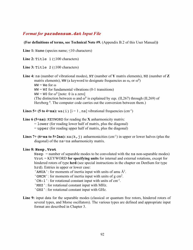
92

Format for paradensum.dat Input File

(For definitions of terms, see Technical Note #9. (Appendix B.2 of this User Manual))

Line 1: Name (species name; ≤10 characters)


Line 3: Title 2 (≤100 characters) Line 4: ns (number of vibrational modes), NY (number of Y matrix elements), NZ (number of Z

matrix elements), WW (a keyword to designate frequencies as ωe or ω0) WW = We for ω WW = Wf for fundamental vibrations (0-1 transitions) WW = W0 for ω0 [note: 0 is a zero] (The distinction between ω and ω0 is explained by eqs. (II,267) through (II,269) of Herzberg 8. The computer code carries out the conversion between them.)




Line 8: Nsep , Vrot Nsep = number of separable modes to be convoluted with the ns non-separable modes) Vrot = KEYWORD for specifying units for internal and external rotations, except for hindered rotors of type hrd (see special instructions in the chapter on DenSum for type hrd). Entries in upper or lower case: 'AMUA': for moments of inertia input with units of amu Å2. 'GMCM': for moments of inertia input with units of g cm2. 'CM-1': for rotational constant input with units of cm-1. 'MHZ': for rotational constant input with MHz. 'GHZ': for rotational constant input with GHz.


93

Line 10: Egrain1, imax1, Isize, Emax2 Egrain1 = energy grain (cm-1) imax1 = number of array elements in lower part of the Double Array (see MultiWell User Manual) Isize = total number elements in the Double Array. Emax2 = upper energy limit

Line 11: chekpoint, <chekname> If chekpoint = "chekstart" (Note the spelling!), then the new calculation

starts by reading the pre-existing checkpoint file (<name>.chk). Otherwise, the full calculation if is carried out. Line 10 must be identical to the data file used to create the pre-existing checkpoint file. <chekname> = filename (≤15 characters) for the checkpoint file to be generated, or

read as input. The filename must contain the suffix, ".chk" and may be different from the name entered on Line 1.

Line 12: (Blank line)

Line 13: nwalkers = number of independent random walks in each window; integer.

Line 14: perc_wind_overlap = percentage of overlap between neighboring windows; real.

Line 15: flatness = flatness criterion for halting the Wang-Landau algorithm: a real number between 0 and 1. The closer to unity, the more accurate is the density of states.

Line 16: writing (writing out Rank<N>.txt files) = 1 (Writing enabled.) = 0 (Writing disabled.)

Line 17: seed_modifier = an integer number which is added to the default random number generator seed in order to get a new random number chain. For usual applications of the code it is set to 0.

Line 18: windbal_key = this keyword sets the windows width. = ”const” (default) windows width is equal for all windows. = ”low” the first two windows are smaller than the others. = ”high” the last two windows are smaller than the others.

Notes

1. Energies are relative to the zero point energy.

2. Be careful when using Gaussian! The Gaussian log file has two sections related to vibrations. The first section is for the usual vibrational analysis to obtain harmonic frequencies. These frequencies are listed from lowest to highest. The second section is for anharmonicities. In the second section, the harmonic frequencies are listed again (along

94

with the fundamental frequencies), but the ordering may not be the same as in the first section. The input for the codes distributed in MultiWell will accept the frequencies in any order, but the ordering of the harmonic frequencies must be consistent with the ordering used for the anharmonicities. For consistency, the Gaussian user must be sure to use the ordering of the harmonic frequencies as listed in association with the anharmonicities in the Gaussian log file.

3. See Sections 1.3 and 1.4 for special instructions for executing paradensum.

8.3 Program sctst (In a future release, sctst will no longer be supported, since it is being replaced by

parsctst, an improved, parallelized version. See Section 8.4.) This program is an implementation16 of the semi-classical transition state theory (SCTST)

formulated by W. H. Miller and coworkers.7,9-11 Our implementation is based on the Wang and Landau algorithm21 and the density of states algorithm of Basire et al.,4 as refined by Nguyen and Barker.14 The literature references should be consulted for further details about the theory, its usefulness, and applications. The literature should be cited as described at the Preface of this User Manual.

The SCTST is a powerful method, since it can be used for computing both thermal (i.e. canonical k(T)) and microcanonical (i.e. k(E)) rate constants, which are essential for master equation calculations. Unlike ordinary transition state theory, the SCTST is fully non-separable: all of the degrees of freedom may be coupled and it is not necessary to assume that the reaction coordinate is separable from the others. It also accounts naturally for zero point energy and for quantum mechanical tunneling along the curved reaction path in hyperdimensional space. In test cases, it is highly accurate.15

The input is similar to that for program bdens (Section 8.1), but it also includes the imaginary frequency and the anharmonicity coefficients associated with the reaction coordinate. The imaginary frequency and the off-diagonal anharmonicity coefficients associated with the reaction coordinate are pure imaginary numbers; the diagonal anharmonicity for the reaction coordinate is a pure real number. These facts affect how the parameters are specified in the input data file sctst.dat. In addition, SCTST as formulated by Miller and coworkers is based on second order vibrational perturbation theory (VPT2).12 Recently, Stanton investigated SCTST based on VPT4 (fourth order perturbation theory) and arrived as a simple correction that is appropriate for symmetrical Eckart barriers.17 To the extent that the actual energy barrier resembles an Eckart barrier, this VPT4 correction improves the performance of SCTST/VPT2. Stanton suggested two slightly different versions of this correction, but the difference between then is small. In program sctst, either of the two corrections (or neither) can be selected by selecting the appropriate key word.

The output files are analogous to the output files from programs bdens and densum. The general output file sctst.out summarizes the input and gives "sums" and "densities" of states for the full energy range specified. These "sums" and "densities" actually correspond to the cumulative reaction probability7,9-11 (CRP) and the corresponding energy derivative, which are equal to the sums and densities in the absence of quantum tunneling. The second output files takes the name of the transition state with ".dens" added: <name>.dens, just as in programs densum and bdens. These files are formatted for use by the MultiWell master equation code. An output file is also generated that gives the thermal partition function (excluding the

95

translations) for the transition state at a set of 100 fixed temperatures (25 K to 3383 K). This file, named <name>.qcrp, is used by program Thermo to calculate canonical rate constants (see Section 6.3 of this User Manual for a description of how the file is used by Thermo).

Running sctst The executable (binary) program resides in the directory

multiwell<version>/bin, where <version> is the version number (e.g. "2014.1b") To execute the compiled program, enter the directory that contains the sctst data file ("sctst.dat") and then type ~/multiwell-<version>/bin/sctst. Directory multiwell<version> is assumed to reside in your Home directory. The output file sctst.out is automatically placed in the directory that contains sctst.dat. A second output file <name>.crp, which is designed to be an input file for the MultiWell master equation code, is also generated, where <name> is the name of the transition state specified in sctst.dat.

sctst has been designed to run using a "checkpoint file" (named <chekname>), which is generated after the density of states of the fully coupled vibrations have been calculated (the most time-consuming part of the calculation). The next part of the calculation convolutes the separable degrees of freedom, if any are specified. The separable degrees of freedom may include free or hindered rotors, harmonic vibrations, etc. In particular, the 1-D external rotation (the K-rotor) and possibly also the 2-D external rotational degrees of freedom may be specified, depending on the application. If desired, the densities of states may be recalculated using various combinations of separable degrees of freedom, but retaining the same set of fully coupled vibrations. Repetitive calculations like these can be restarted using the checkpoint file, which saves considerable computer time.

Another reason for running repetitive calculations by starting with the checkpoint file is because whenever the reaction threshold energy is changed, the SCTST requires that the density of states of the transition state and the cumulative reaction probability be recalculated.16 Adjusting reaction barriers to fit experimental data may require multiple repetitive calculations, and restarting by using the checkpoint file will reduce the computer time by an order of magnitude or more.

In summary, four output files are generated by sctst: sctst.out, <name>.crp, <chekname> (which must include the .chk suffix), and <name>.qcrp. The first file (sctst.out) is a standard output file, which summarizes all input and output. The second file (<name>.chk), which takes a chemical species name as part of the file name, is the checkpoint file, which is an important time-saving measure for subsequent runs using the same vibrational parameters, as described in the preceding paragraph. The third file (<name>.crp), tabulates the cumulative reaction probability (CRP) and its energy derivative (analogous to sums and densities of states), formatted as double arrays; it is formatted for use as input for the MultiWell master equation code. By using this input file, master equation calculations can be carried out with microcanonical rate constants (i.e. k(E)) computed by including the fully-coupled vibrations. The fourth file (<name>.qcrp) is formatted as a supplementary input file for program Thermo; it tabulates the partition function for the CRP and other thermodynamic properties of the coupled vibrational modes at a set of fixed temperatures from 50 K to >3000 K. Thermo can utilize these partition functions to compute thermal rate constants using the SCTST. See Section 6.3 of this User Manual for a description.

96

Data File Format

(For definitions of terms, see Technical Note B.9 and Nguyen et al.16 )

Line 1: Name (transition state name; ≤10 characters)


Line 3: Title 2 (≤100 characters) Line 4: ns (number of orthogonal vibrational modes, not including the reaction coordinate), NY (number of Y matrix elements), NZ (number of Z matrix elements), WW (a keyword to designate frequencies as ωe or ω0) WW = We for ω WW = Wf for fundamental vibrations (0-1 transitions) WW = W0 for ω0 [note: 0 is a zero]





Line 8: Nsep , Vrot Nsep = number of active separable modes (as in Line 5 of Densum) to be convoluted with the ns non-separable modes entered above) Vrot = KEYWORD for specifying units for internal and external rotations, except for hindered rotors of type hrd (see special instructions in the chapter on DenSum for type hrd). Entries in upper or lower case:

Vrot Keywords: 'AMUA': for moments of inertia input with units of amu Å2. 'GMCM': for moments of inertia input with units of g cm2. 'CM-1': for rotational constant input with units of cm-1. 'MHZ': for rotational constant input with MHz. 'GHZ': for rotational constant input with GHz.


97

Line 10: Egrain1, imax1, Isize, Emax2, KEYWORD1 Egrain1 = energy grain (cm-1) imax1 = number of array elements in lower part of the Double Array (see MultiWell User Manual) Isize = total number elements in the Double Array. Emax2 = upper energy limit KEYWORD1 = controls number of stochastic trials (note that execution time is

proportional to the number of trials): Fair: low statistical accuracy (102 trials per energy grain) Good: good statistical accuracy (103 trials per energy grain). Better: better statistical accuracy (104 trials per energy grain) Best: best statistical accuracy (105 trials per energy grain) Extra: best statistical accuracy (106 trials per energy grain, but no more than

2´109 total trials for all energy grains)

Line 11: KEYWORD "checkpoint", <chekname> If "chekpoint" = "chekstart" (Note the spelling!), then the new calculation starts

by reading a pre-existing checkpoint file. Otherwise, the full calculation is carried out, including generation of a new checkpoint file. All data from Line 2 through Line 10, inclusive, must be identical to the data file used to create the pre-existing checkpoint file in the first place.

<chekname> = filename (≤15 characters) for the checkpoint file to be generated, or read as input. The filename must contain the suffix, ".chk" and may be different from the name entered on Line 1.

Line 12: KEYWORD3

KEYWORD3 = controls number of samples for the semi-classical calculation (typically the same as KEYWORD1). The samples are used to compute average quantities employed by the theory.

Fair: low accuracy (102 samples per energy grain) Good: good accuracy (103 samples per energy grain). Better: better accuracy (104 samples per energy grain) Best: best accuracy (105 samples per energy grain) Extra: best accuracy (106 samples per energy grain, but no more than 2´109 total

samples for all energy grains)

Line 13: KEYWORD "VPTx" New Feature in 2017; this line must be added to older files that are run using 2017 version, or newer. VPTx = controls corrections to the basic SCTST/VP2.

VPT2: no correction. VPT4A: Recommended. VPT4 correction (Eq. 42 in the paper by Stanton.17) VPT4B: VPT4 correction (Eq. 37 in the paper by Stanton.17)

Line 14: Vf , Vr , Eunits

98

Barrier heights (including zero point energy corrections) in forward (Vf) and reverse (Vr) directions, and their energy units (Eunits: kcal, kjou, or cm-1)

Line 15: vimag, Xff Imaginary frequency and the diagonal anharmonicity coefficient for the reaction coordinate (units of cm-1)

Line 16: Xkf Off-diagonal anharmonicity coefficients (units of cm-1) multiplied by i = (-1)1/2: ns of them, in order. Since the Xk,F coefficients are pure imaginary, they can be written

, where is a real number. The quantities to be input are

, which is in the same format as GAUSSIAN output. In

contrast, CFOUR output gives Xk,F expressed as followed by the symbol "i", i.e. "

i". These conventions are equivalent, but it is easy to make a sign error. Be careful!

Notes


2. In second order vibrational perturbation theory (VPT2), the zero point energy (ZPE) includes contributions from the harmonic frequencies, the anharmonicities, but it does NOT include the harmonic imaginary frequency or any of the anharmonicity coefficients involving the imaginary frequency. The ZPE also includes an additional term denoted G0 (see Eq. 9 in Appendix B.9),13,19 which cancels-out in spectroscopy applications but must be included for every species in high-accuracy thermochemistry and kinetics calculations. The value of G0 must be computed by electronic structure programs employing VPT2 (e.g. GAUSSIAN and CFOUR), and is not computed by MultiWell itself. For ab initio kinetics calculations involving chemical species and transition states with large rotational constants, G0 may be significant, but it is very small for molecules with small rotational constants. For high accuracy ab initio kinetics calculations (e.g. Ref. 16, G0 can be included manually by modifying the reaction critical energy (which already includes zero point energy corrections).

3. Be careful when using Gaussian! The Gaussian log file has two sections related to vibrations. The first section is for the usual vibrational analysis to obtain harmonic frequencies. These frequencies are listed from lowest to highest. The second section is for anharmonicities. In the second section, the harmonic frequencies are listed again (along with the fundamental frequencies), but the ordering may not be the same as in the first section. The input for the codes distributed in MultiWell will accept the frequencies in any order, but the ordering of the harmonic frequencies must be consistent with the ordering used for the anharmonicities. For consistency, the Gaussian user must be sure to use the ordering of the harmonic frequencies as listed in association with the anharmonicities in the Gaussian log file.

Xk ,F = i Xk ,F

Xk ,F

i ⋅ Xk ,F = i ⋅ i Xk ,F = − Xk ,F

Xk ,F

Xk ,F

99

8.4 Program parsctst parsctst: parallel and improved version of sctst (in a future release, sctst will no

longer be supported.) Program Authors:

parsctst: C. Aieta, F. Gabas, and M. Ceotto sctst: T. L. Nguyen and J. R. Barker

Contact: Michele Ceotto: [email protected] This program is an implementation19 of the semi-classical transition state theory (SCTST)

formulated by W. H. Miller and coworkers.10,12-14 Our implementation is based on the Wang and Landau algorithm25 and the density of states algorithm of Basire et al.,3 as refined by Nguyen and Barker.17 The literature references should be consulted for further details about the theory, its usefulness, and applications. The literature should be cited as described at the Preface of this User Manual.

The SCTST is a powerful method, since it can be used for computing both thermal (i.e. canonical k(T)) and microcanonical (i.e. k(E)) rate constants, which are essential for master equation calculations. Unlike ordinary transition state theory, the SCTST is fully non-separable: all of the degrees of freedom may be coupled and it is not necessary to assume that the reaction coordinate is separable from the others. It also accounts naturally for zero point energy and for quantum mechanical tunneling along the curved reaction path in hyperdimensional space. In test cases, it is highly accurate.18

paradensum is a parallel code2 that can exploit not only single but also multiple core architectures. In this way the computation of the density of states is significantly accelerated when considering high dimensionality systems. The parallelization strategy is to divide the energy range into energy “windows” and set the calculations of G(Ei) for each window on a single processor. This strategy is dictated by the observation that less random sampling events and reduced computational effort is needed for Monte Carlo to converge in a restricted energy range.

The number of processors is given by the windowing choice and, by default, all windows have the same width. This setting can be changed by modifying the appropriate keyword in the input file. If the computational time spent by each window to reach the flatness criterion is unbalanced, the code prints a warning in the Windows_info.txt output file. Then, the user can decide to halve the width of the first two or the last two windows.

Since the Wang-Landau density of states is notoriously biased at the edges of small energy windows, we always keep a percentage of overlap between neighbor windows. This is also necessary for the normalization of the G(Ei) obtained in each window to give the complete function on the whole energy domain. The code supports the possibility to run serially multiple walkers in each energy window. This feature improves the statistics of sampling in each window but does not have any impact on the speedup. To run the code the user has to supply the number of processors that is equal to the number of windows and a percentage of overlap between them as input parameters. When the number of processors (windows) is set to unity, then paradensum will run in serial mode (i.e. it can run on a single cpu or core). The set up of the input file for these parameters is described below. For a full description of the parsctst implementation, see the paper by Aieta, Gabas and Ceotto.2

The input is similar to that for programs bdens (Section 8.1), and paradensum (Section 8.2) but it also includes the imaginary frequency and the anharmonicity coefficients

100

associated with the reaction coordinate. The imaginary frequency and the off-diagonal anharmonicity coefficients associated with the reaction coordinate are pure imaginary numbers; the diagonal anharmonicity for the reaction coordinate is a pure real number. These facts affect how the parameters are specified in the input data file parctst.dat. In addition, SCTST as formulated by Miller and coworkers is based on second order vibrational perturbation theory (VPT2).15 Recently, Stanton investigated SCTST based on VPT4 (fourth order perturbation theory) and arrived as a simple correction that is appropriate for symmetrical Eckart barriers.20 To the extent that the actual energy barrier resembles an Eckart barrier, this VPT4 correction improves the performance of SCTST/VPT2. Stanton suggested two slightly different versions of this correction, but the difference between then is small. In program parctst, either of the two corrections (or neither) can be selected by selecting the appropriate key word.

The output files are analogous to the output files from programs paradensum, bdens and densum. The general output file parctst.out summarizes the input and gives "sums" and "densities" of states for the full energy range specified. These "sums" and "densities" actually correspond to the cumulative reaction probability10,12-14 (CRP) and the corresponding energy derivative, which are identified with the sums and densities in the absence of quantum tunneling. The second output file takes the name of the transition state with ".crp" added: <name>.crp, just as in programs densum, bdens and paradensum. These files are formatted for use by the MultiWell master equation code. An output file is also generated that gives the thermal partition function (excluding the translations) for the transition state at a set of 100 fixed temperatures (1 K to 3383 K). This file, named <name>.qcrp, is used by program Thermo to calculate canonical rate constants (see Section 6.3 of this User Manual for a description of how the file is used by Thermo).

Running parsctst Parsctst is a parallel code. To compile and run the code, it is necessary to have

previously installed supplementary software. Details are given in Section 1.4. sctst has been designed to run using a "checkpoint file" (named <chekname>),

which is generated after the density of states of the fully coupled vibrations have been calculated (the most time-consuming part of the calculation). The next part of the calculation convolutes the separable degrees of freedom, if any are specified. The separable degrees of freedom may include free or hindered rotors, harmonic vibrations, etc. In particular, the 1-D external rotation (the K-rotor) and possibly also the 2-D external rotational degrees of freedom may be specified, depending on the application. If desired, the densities of states may be recalculated using various combinations of separable degrees of freedom, but retaining the same set of fully coupled vibrations. Repetitive calculations like these can be restarted using the checkpoint file, which saves considerable computer time. Note that when using the checkpoint file, it is not necessary to run the code in parallel mode.

Another reason for running repetitive calculations by starting with the checkpoint file is because whenever the reaction threshold energy is changed, the SCTST requires that the cumulative reaction probability be recalculated.19 Adjusting reaction barriers to fit experimental data may require multiple repetitive calculations, and restarting by using the checkpoint file will reduce the computer time by an order of magnitude or more.

The input data file parsctst.dat includes molecular parameters for computing the cumulative reaction probablility, as well as parallel execution parameters. Directory multiwell-<version> is assumed to reside in your Home directory. Execution of

101

parsctst is carried out within the directory that contains the input data file parsctst.dat. All of the output files are automatically placed in the directory that contains parsctst.dat.

In summary, five output files are generated by parctst: parctst.out, <name>.crp, <chekname> (which must include the .chk suffix), and <name>.qcrp. , and Windows_info.txt. The first file (parctst.out) is a standard output file, which summarizes all input and output. The second file (<chkname>), which takes a chemical species name as part of the file name, is the checkpoint file, which is an important time-saving measure for subsequent runs using the same vibrational parameters, as described in the preceding paragraph. The third file (<name>.crp), tabulates the cumulative reaction probability (CRP) and its energy derivative (analogous to sums and densities of states), formatted as double arrays for use as input for the MultiWell master equation code. By using this input file, master equation calculations can be carried out with microcanonical rate constants (i.e. k(E)) computed by including the fully-coupled vibrations. The fourth file (<name>.qcrp) is formatted as a supplementary input file for program Thermo; it tabulates the partition function for the CRP and other thermodynamic properties of the coupled vibrational modes at a set of fixed temperatures from 50 K to >3000 K. Thermo can utilize these partition functions to compute thermal rate constants using the SCTST. See Section 6.3 of this User Manual for a description.

The file Windows_info.txt contains details about windows division, i.e. the total number of energy grains, the number of energy grains in each window after the overlap has been added, and the low and high energy boundaries of each window.

Users may also select a supplementary writing option, which generates a file called Rank<N>.txt for each parallel process (here, <N> is an integer number that identifies the process). These files report all details about the Wang-Landau algorithm executed by each parallel process. Users may freely enable or disable writing the Rank<N>.txt files, which are intended as a user check on parallel execution.

Format for parsctst.dat Input File

(For definitions of terms, see Technical Note B.9 and Nguyen et al.19 )

Line 1: Name (transition state name; ≤10 characters)


Line 3: Title 2 (≤100 characters) Line 4: ns (number of orthogonal vibrational modes, not including the reaction coordinate), NY (number of Y matrix elements), NZ (number of Z matrix elements), WW (a keyword to designate frequencies as ωe or ω0) WW = We for ω WW = Wf for fundamental vibrations (0-1 transitions) WW = W0 for ω0 [note: 0 is a zero]


102




Line 8: Nsep , Vrot Nsep = number of active separable modes (as in Line 5 of Densum) to be convoluted with the ns non-separable modes entered above) Vrot = KEYWORD for specifying units for internal and external rotations, except for hindered rotors of type hrd (see special instructions in the chapter on DenSum for type hrd). Entries in upper or lower case:

Vrot Keywords: 'AMUA': for moments of inertia input with units of amu Å2. 'GMCM': for moments of inertia input with units of g cm2. 'CM-1': for rotational constant input with units of cm-1. 'MHZ': for rotational constant input with MHz. 'GHZ': for rotational constant input with GHz.


Line 10: Egrain1, imax1, Isize, Emax2 Egrain1 = energy grain (cm-1) imax1 = number of array elements in lower part of the Double Array (see MultiWell User Manual) Isize = total number elements in the Double Array. Emax2 = upper energy limit

Line 11: KEYWORD "checkpoint", <chekname> If "chekpoint" = "chekstart" (Note the spelling!), then the new calculation starts

by reading a pre-existing checkpoint file. Otherwise, the full calculation is carried out, including generation of a new checkpoint file. All data from Line 2 through Line 10, inclusive, must be identical to the data file used to create the pre-existing checkpoint file in the first place.

<chekname> = filename (≤15 characters) for the checkpoint file to be generated, or read as input. The filename must contain the suffix, ".chk" and may be different from the name entered on Line 1.

Line 12: KEYWORD "VPTx" New Feature in 2017; this line must be added to older files that are run using 2017 version, or newer. VPTx = controls corrections to the basic SCTST/VP2.

103

VPT2: no correction. VPT4A: Recommended. VPT4 correction (Eq. 42 in the paper by Stanton.20) VPT4B: VPT4 correction (Eq. 37 in the paper by Stanton.20)

Line 14: Vf , Vr , Eunits Barrier heights (including zero point energy corrections) in forward (Vf) and reverse (Vr) directions, and their energy units (Eunits: kcal, kjou, or cm-1)

Line 15: vimag, Xff Imaginary frequency and the diagonal anharmonicity coefficient for the reaction coordinate (units of cm-1)

Line 16: Xkf Off-diagonal anharmonicity coefficients (units of cm-1) multiplied by i = (-1)1/2: ns of them, in order. Since the Xk,F coefficients are pure imaginary, they can be written

, where is a real number. The quantities to be input are

, which is in the same format as GAUSSIAN output. In

contrast, CFOUR output gives Xk,F expressed as followed by the symbol "i", i.e. "

i". These conventions are equivalent, but it is easy to make a sign error. Be careful!

Line 17: (Blank line)

Line 18: nwalkers = number of independent random walks in each window; integer.

Line 19: perc_wind_overlap = percentage of overlap between neighboring windows; real.

Line 20: flatness = flatness criterion for halting the Wang-Landau algorithm: a real number between 0 and 1. The closer to unity, the more accurate is the density of states.

Line 21: writing (writing out Rank<N>.txt files) = 1 (Writing enabled.) = 0 (Writing disabled.)

Line 22: seed_modifier = an integer number which is added to the default random number generator seed in order to get a new random number chain. For usual applications of the code it is set to 0.

Line 23: windbal_key = this keyword sets the windows width. = ”const” (default) windows width is equal for all windows. = ”low” the first two windows are smaller than the others. = ”high” the last two windows are smaller than the others.

Xk ,F = i Xk ,F

Xk ,F

i ⋅ Xk ,F = i ⋅ i Xk ,F = − Xk ,F

Xk ,F

Xk ,F

104

Notes


2. In second order vibrational perturbation theory (VPT2), the zero point energy (ZPE) includes contributions from the harmonic frequencies, the anharmonicities, but it does NOT include the harmonic imaginary frequency or any of the anharmonicity coefficients involving the imaginary frequency. The ZPE also includes an additional term denoted G0 (see Eq. 9 in Appendix B.9),16,23 which cancels-out in spectroscopy applications but must be included for every species in high-accuracy thermochemistry and kinetics calculations. The value of G0 must be computed by electronic structure programs employing VPT2 (e.g. GAUSSIAN and CFOUR), and is not computed by MultiWell itself. For ab initio kinetics calculations involving chemical species and transition states with large rotational constants, G0 may be significant, but it is very small for molecules with small rotational constants. For high accuracy ab initio kinetics calculations (e.g. Ref. 19, G0 can be included manually by modifying the reaction critical energy (which already includes zero point energy corrections).

3. Be careful when using Gaussian! The Gaussian log file has two sections related to vibrations. The first section is for the usual vibrational analysis to obtain harmonic frequencies. These frequencies are listed from lowest to highest. The second section is for anharmonicities. In the second section, the harmonic frequencies are listed again (along with the fundamental frequencies), but the ordering may not be the same as in the first section. The input for the codes distributed in MultiWell will accept the frequencies in any order, but the ordering of the harmonic frequencies must be consistent with the ordering used for the anharmonicities. For consistency, the Gaussian user must be sure to use the ordering of the harmonic frequencies as listed in association with the anharmonicities in the Gaussian log file.

References (1) Aieta, C.; Gabas, F.; Ceotto, M. An Efficient Computational Approach for the

Calculation of the Vibrational Density of States. J. Phys. Chem. A. 2016, DOI: 10.1021/acs.jpca.1025b12364; DOI: 10.1021/acs.jpca.5b12364.

(2) Aieta, C.; Gabas, F.; Ceotto, M. Parallel Implementation of Semiclassical Transition State Theory. J. Chem. Theory Comput. 2019, 15, 2143-2153; DOI: 10.1021/acs.jctc.8b01286.

(3) Barker, J. R. Sums of Quantum States for Non–Separable Degrees of Freedom: Multidimensional Monte Carlo Integration. J. Phys. Chem. 1987, 91, 3849-3854.

(4) Basire, M.; Parneix, P.; Calvo, F. Quantum anharmonic densities of states using the Wang-Landau method. J. Chem. Phys. 2008, 129, 081101.


(6) Cané, E.; Miani, A.; Trombetti, A. Anharmonic Force Fields of Naphthalene-h8 and Naphthalene-d8. J. Phys. Chem. A. 2007, 111, 8218-8222.

105


(8) Herzberg, G. Molecular Spectra and Molecular Structure. II. Infrared and Raman Spectra, 2 ed.; Van Nostrand Reinhold Co.: Cincinnati, 1945.

(9) Miller, J. H. The kinetics of polynuclear aromatic hydrocarbon agglomeration in flames. Proc. Combust. Inst. 1990, 23.



(12) Mills, I. M. Modern Spectroscopy; Modern Research; Academic Press: New York, NY, 1972.

(13) Mills, I. M. Vibration-Rotation Structure in Asymmetric- and Symmetric-Top Molecules. In Molecular Spectroscopy: Modern Research; Rao, K. N., Mathews, C. W., Eds.; Academic Press: New York, 1972; Vol. 1; pp 115-140.


(15) Nguyen, T. L.; Barker, J. R.; Stanton, J. F. Atmospheric Reaction Rate Constants and Kinetic Isotope Effects Computed Using the HEAT Protocol and Semi-Classical Transition State Theory. In Advances in Atmospheric Chemistry; Barker, J. R., Steiner, A. L., Wallington, T. J., Eds.; World Scientific: Singapore, 2017; Vol. 1; pp 403-492.


(17) Stanton, J. F. Semiclassical Transition-State Theory Based on Fourth-Order Vibrational Perturbation Theory: The Symmetrical Eckart Barrier. J. Phys. Chem. Lett. 2016, 7, 2708-2713.


(19) Truhlar, D. G.; Isaacson, A. D. Simple perturbation theory estimates of equilibrium constants from force fields. J. Chem. Phys. 1990, 94, 357-359.

(20) Wang, F.; Landau, D. P. Determining the density of states for classical statistical models: A random walk algorithm to produce a fat histogram. Phys. Rev. E 2001, 64, 056101-056101.

(21) Wang, F.; Landau, D. P. Efficient, Multiple-Range Random Walk Algorithm to Calculate the Density of States. Phys. Rev. Letters 2001, 86, 2050-2053.

106

9. lamm: Effective Mass for Internal Rotation lamm: Large Amplitude Motion Mass Program Author: Thanh Lam Nguyen Contact: [email protected]

9.1 Introduction This program is a tool for obtaining the effective mass (as a function of angle or distance)

for large amplitude motions, such as internal rotation. The output is used as part of the input data file needed for computing sums and densities of states (using program DenSum) and partition functions (program Thermo).

Program lamm uses the ro-vibrational G matrix-based algorithm described in the papers of Harthcock et al.3,4 and others to compute the effective reduced mass for one-dimensional torsions and other large amplitude motions, which are assumed to be separable from the other molecular degrees of freedom.

Molecular geometries can be computed at discrete values of χ by using any of the many available quantum chemistry codes, such as Gaussian,2 Molpro,6 CFour,5 etc. Program lamm is intended to help users compute the torsion rotational constant Bhr(χ) and the potential energy V(χ), based on the output from the quantum chemistry program.

For hindered internal rotation, lamm employs Cartesian coordinates obtained from quantum chemical calculations carried out as a function of the dihedral angle χ (0≤χ<2p). The output of lamm consists of the torsion rotational constant function Bhr(χ) (or the corresponding moment of inertia function I(χ)) tabulated as a function of χ. The potential energy can also be obtained from the quantum chemistry calculations and expressed as a function of χ. These functions must then be fitted by the user to any one of the several truncated Fourier series that are recognized by DenSum and Thermo (see the MultiWell User Manual). The Fourier coefficients are used by programs DenSum and Thermo to solve the Schrödinger equation for the energy eigenstates (see Appendix B.8), which are needed to compute densities of states and partition functions, respectively.

A script is provided to assist users in extracting the required information from Gaussian output files (see Section 9.7).

9.2 Compiling and Running lamm The source directory for lamm resides in the MultiWell src directory. The program is

compiled on Linux by entering the MultiWell directory and typing “make” (omit the quotation marks), followed by a carriage return. The executable file is stored in the MultiWell bin directory. The default compiler is gfortran. The compiler can be changed by revising lines in file src/lamm/Makefile. To remove old object files and executables, enter directory src/lamm and type “make clean”, followed by a carriage return.

To execute the compiled program, enter the directory that contains the lamm data file (“lamm.dat”) and then type ~/multiwell-<version>/bin/lamm, where <version> refers to the multiwell version number (e.g. "2010.0"). This command executes the binary executable file. The output file (“lamm.out”) is automatically placed in the directory that contains lamm.dat.

107

9.3 Notes and Limits For the current version of the lamm program, Cartesian coordinates of optimized

geometries must be obtained by constrained optimizations. When using Gaussian, the keyword “NOSYM” and/or OPT=”Z-Matrix”, or the equivalent must be specified.

The lamm program does not automatically identify the molecular symmetry; it always assumes that the molecule has no symmetry (C1 symmetry). Therefore the effective reduced moment of inertia will be computed only for the number of optimized geometries that are input.

Since the derivatives of the nuclear positions with respect to the torsional coordinate are computed by central finite differences, a fairly small torsional angle step-size must be used in order to achieve numerical accuracy. In our experience, a step-size of ≤10° is a good choice for most purposes.

In addition to torsional motions, the lamm program can be used for computing the effective mass for other separable large-amplitude vibrational motions. Specific implementations will be added in the future.

Users may be interested in program I_Eckart, which was coded in MATLAB by Wong, Thom and Field 7. We would like to thank Dr. Wong and Prof. Field for useful discussions and for providing a copy of their program, which we used for benchmarks.

9.4 Data File Format

Line 1: Name of molecule (≤ 100 characters)

Line 2: Title (≤ 100 characters)

Line 3: Natom (number of atoms in molecule)

Line 4: Amin (lower limit of torsion angle in degrees), M (number of optimized geometries), DELA (step-size of torsion angle in degrees).

Line 5+ (lines 5 to 4 + N): list of atomic masses (in amu)

Line 6+ (lines 5 + N to 4 + N + N*M): list of Cartesian coordinates (in Angstroms) for M optimized geometries as a function of the torsion dihedral angle.

Line 7 (lines 5 + N + N*M): comment line (≤100 characters)

Line 8+ (lines 6 + N + N*M to 5 + N + N*M + M): list of torsional angle (in degrees) and relative energies (in cm-1).

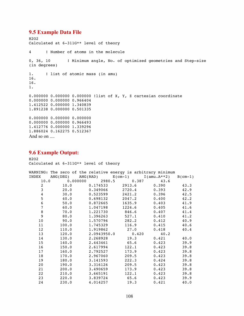
108

9.5 Example Data File H2O2 Calculated at 6-311G** level of theory 4 ! Number of atoms in the molecule 0, 36, 10 ! Minimum angle, No. of optimized geometries and Step-size (in degrees) 1. ! list of atomic mass (in amu) 16. 16. 1. 0.000000 0.000000 0.000000 !list of X, Y, Z cartesian coordinate 0.000000 0.000000 0.966404 1.412522 0.000000 1.340839 1.891238 0.000000 0.501335 0.000000 0.000000 0.000000 0.000000 0.000000 0.966493 1.412776 0.000000 1.339296 1.886024 0.162275 0.512367 And so on ....

9.6 Example Output: H2O2 Calculated at 6-311G** level of theory WARNING: The zero of the relative energy is arbitrary minimum INDEX ANG(DEG) ANG(RAD) E(cm-1) I(amu.A**2) B(cm-1) 10.0 0.000000 2980.5 0.387 43.6 2 10.0 0.174533 2913.6 0.390 43.3 3 20.0 0.349066 2720.4 0.393 42.9 4 30.0 0.523599 2421.2 0.396 42.5 5 40.0 0.698132 2047.2 0.400 42.2 6 50.0 0.872665 1635.9 0.403 41.9 7 60.0 1.047198 1224.6 0.405 41.6 8 70.0 1.221730 846.6 0.407 41.4 9 80.0 1.396263 527.1 0.410 41.2 10 90.0 1.570796 282.2 0.412 40.9 11 100.0 1.745329 116.9 0.415 40.6 12 110.0 1.919862 27.0 0.418 40.4 13 120.0 2.0943950.0 0.420 40.2 14 130.0 2.268928 19.3 0.421 40.0 15 140.0 2.443461 65.6 0.423 39.9 16 150.0 2.617994 122.1 0.423 39.8 17 160.0 2.792527 173.9 0.423 39.8 18 170.0 2.967060 209.5 0.423 39.8 19 180.0 3.141593 222.3 0.424 39.8 20 190.0 3.316126 209.5 0.423 39.8 21 200.0 3.490659 173.9 0.423 39.8 22 210.0 3.665191 122.1 0.423 39.8 23 220.0 3.839724 65.6 0.423 39.9 24 230.0 4.014257 19.3 0.421 40.0

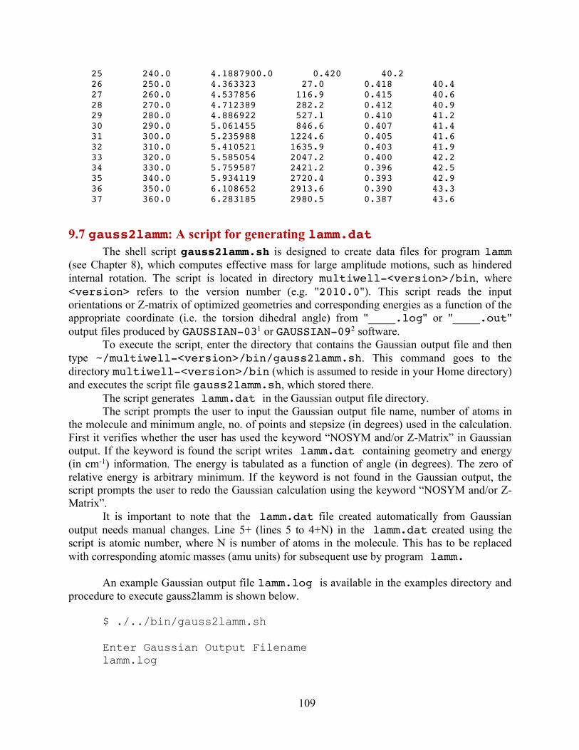
109

25 240.0 4.1887900.0 0.420 40.2 26 250.0 4.363323 27.0 0.418 40.4 27 260.0 4.537856 116.9 0.415 40.6 28 270.0 4.712389 282.2 0.412 40.9 29 280.0 4.886922 527.1 0.410 41.2 30 290.0 5.061455 846.6 0.407 41.4 31 300.0 5.235988 1224.6 0.405 41.6 32 310.0 5.410521 1635.9 0.403 41.9 33 320.0 5.585054 2047.2 0.400 42.2 34 330.0 5.759587 2421.2 0.396 42.5 35 340.0 5.934119 2720.4 0.393 42.9 36 350.0 6.108652 2913.6 0.390 43.3 37 360.0 6.283185 2980.5 0.387 43.6

9.7 gauss2lamm: A script for generating lamm.dat The shell script gauss2lamm.sh is designed to create data files for program lamm

(see Chapter 8), which computes effective mass for large amplitude motions, such as hindered internal rotation. The script is located in directory multiwell-<version>/bin, where <version> refers to the version number (e.g. "2010.0"). This script reads the input orientations or Z-matrix of optimized geometries and corresponding energies as a function of the appropriate coordinate (i.e. the torsion dihedral angle) from "____.log" or "____.out" output files produced by GAUSSIAN-031 or GAUSSIAN-092 software.

To execute the script, enter the directory that contains the Gaussian output file and then type ~/multiwell-<version>/bin/gauss2lamm.sh. This command goes to the directory multiwell-<version>/bin (which is assumed to reside in your Home directory) and executes the script file gauss2lamm.sh, which stored there.

The script generates lamm.dat in the Gaussian output file directory. The script prompts the user to input the Gaussian output file name, number of atoms in

the molecule and minimum angle, no. of points and stepsize (in degrees) used in the calculation. First it verifies whether the user has used the keyword “NOSYM and/or Z-Matrix” in Gaussian output. If the keyword is found the script writes lamm.dat containing geometry and energy (in cm-1) information. The energy is tabulated as a function of angle (in degrees). The zero of relative energy is arbitrary minimum. If the keyword is not found in the Gaussian output, the script prompts the user to redo the Gaussian calculation using the keyword “NOSYM and/or Z-Matrix”.

It is important to note that the lamm.dat file created automatically from Gaussian output needs manual changes. Line 5+ (lines 5 to 4+N) in the lamm.dat created using the script is atomic number, where N is number of atoms in the molecule. This has to be replaced with corresponding atomic masses (amu units) for subsequent use by program lamm.

An example Gaussian output file lamm.log is available in the examples directory and

procedure to execute gauss2lamm is shown below. $ ./../bin/gauss2lamm.sh Enter Gaussian Output Filename lamm.log

110

Keyword NOSYM found in the output Enter total number of atoms in the molecule 5 Enter MIN angle, No. of Points and Stepsize in degrees used in the calculation 0 36 10 Proceeding to collect data from lamm.log Lowest energy in the surface scan: -740.457504043 hartrees

111

References

(1) Frisch, M. J.; Trucks, G. W.; Schlegel, H. B.; Scuseria, G. E.; Robb, M. A.; Cheeseman, J. R.; Montgomery, J. A., Jr.; Vreven, T.; Kudin, K. N.; Burant, J. C.; Millam, J. M.; Iyengar, S. S.; Tomasi, J.; Barone, V.; Mennucci, B.; Cossi, M.; Scalmani, G.; Rega, N.; Petersson, G. A.; Nakatsuji, H.; Hada, M.; Ehara, M.; Toyota, K.; Fukuda, R.; Hasegawa, J.; Ishida, M.; Nakajima, T.; Honda, Y.; Kitao, O.; Nakai, H.; Klene, M.; Li, X.; Knox, J. E.; Hratchian, H. P.; Cross, J. B.; Bakken, V.; Adamo, C.; Jaramillo, J.; Gomperts, R.; Stratmann, R. E.; Yazyev, O.; Austin, A. J.; Cammi, R.; Pomelli, C.; Ochterski, J. W.; Ayala, P. Y.; Morokuma, K.; Voth, G. A.; Salvador, P.; Dannenberg, J. J.; Zakrzewski, V. G.; Dapprich, S.; Daniels, A. D.; Strain, M. C.; Farkas, O.; Malick, D. K.; Rabuck, A. D.; Raghavachari, K.; Foresman, J. B.; Ortiz, J. V.; Cui, Q.; Baboul, A. G.; Clifford, S.; Cioslowski, J.; Stefanov, B. B.; Liu, G.; Liashenko, A.; Piskorz, P.; Komaromi, I.; Martin, R. L.; Fox, D. J.; Keith, T.; Al-Laham, M. A.; Peng, C. Y.; Nanayakkara, A.; Challacombe, M.; Gill, P. M. W.; Johnson, B.; Chen, W.; Wong, M. W.; Gonzalez, C.; Pople, J. A. Gaussian 03, Revision C.02; Gaussian, Inc.: Wallingford CT, 2004.

(2) Frisch, M. J.; Trucks, G. W.; Schlegel, H. B.; Scuseria, G. E.; Robb, M. A.; Cheeseman, J. R.; Scalmani, G.; Barone, V.; Mennucci, B.; Petersson, G. A.; Nakatsuji, H.; Caricato, M.; Li, X.; Hratchian, H. P.; Izmaylov, A. F.; Bloino, J.; Zheng, G.; Sonnenberg, J. L.; Hada, M.; Ehara, M.; Toyota, K.; Fukuda, R.; Hasegawa, J.; Ishida, M.; Nakajima, T.; Honda, Y.; Kitao, O.; Nakai, H.; Vreven, T.; J. A. Montgomery, J.; Peralta, J. E.; Ogliaro, F.; Bearpark, M.; Heyd, J. J.; Brothers, E.; Kudin, K. N.; Staroverov, V. N.; Kobayashi, R.; Normand, J.; Raghavachari, K.; Rendell, A.; Burant, J. C.; Iyengar, S. S.; Tomasi, J.; Cossi, M.; Rega, N.; Millam, J. M.; Klene, M.; Knox, J. E.; Cross, J. B.; Bakken, V.; Adamo, C.; Jaramillo, J.; Gomperts, R.; Stratmann, R. E.; Yazyev, O.; Austin, A. J.; Cammi, R.; Pomelli, C.; Ochterski, J. W.; Martin, R. L.; Morokuma, K.; Zakrzewski, V. G.; Voth, G. A.; Salvador, P.; Dannenberg, J. J.; Dapprich, S.; Daniels, A. D.; Farkas, O.; Foresman, J. B.; Ortiz, J. V.; Cioslowski, J.; Fox, D. J. Gaussian 09, Revision A.1; Revision A.1 ed.; Gaussian, Inc.: Wallingford CT, 2009.

(3) Harthcock, M. A.; Laane, J. Calculation of kinetic energy terms for the vibrational Hamiltonian: Application to large-amplitude vibrations using one-, two-, and three-dimensional models. J. Mol. Spectros. 1982, 91, 300-324.

(4) Harthcock, M. A.; Laane, J. Calculation of two-dimensional vibrational potential energy surfaces utilizing prediagonalized basis sets and Van Vleck perturbation methods. J. Phys. Chem. 1985, 89, 4231–4240.

(5) Stanton, J. F.; Gauss, J.; Harding, M. E.; Szalay, P. G.; Auer, w. c. f. A. A.; Bartlett, R. J.; Benedikt, U.; Berger, C.; Bernholdt, D. E.; Bomble, Y. J.; Christiansen, O.; Heckert, M.; Heun, O.; Huber, C.; Jagan, T.-C.; Jonsson, D.; Jusélius, J.; Klein, K.; Lauderdale, W. J.; Matthews, D. A.; Metzroth, T.; O'Neill, D. P.; Price, D. R.; Prochnow, E.; Ruud, K.; Schiffmann, F.; Stopkowicz, S.; Vázquez, J.; Wang, F.; Watts, J. D. and the integral packages MOLECULE (J. Almlöf and P.R. Taylor); PROPS (P.R. Taylor); ABACUS (T. Helgaker, H.J. Aa. Jensen, P. Jørgensen, and J. Olsen); and ECP routines by A. V. Mitin

112

and C. van Wüllen. CFOUR, a quantum chemical program package (www.cfour.de/), 2009.

(6) Werner, H.-J.; Knowles, P. J.; Lindh, R.; Manby, F. R.; Schütz, M.; Celani, P.; Korona, T.; Rauhut, G.; Amos, R. D.; Bernhardsson, A.; Berning, A.; Cooper, D. L.; Deegan, M. J. O.; Dobbyn, A. J.; Eckert, F.; Hampel, C.; Hetzer, G.; Lloyd, A. W.; McNicholas, S. J.; W. Meyer, W.; Mura, M. E.; Nicklass, A.; Palmieri, P.; Pitzer, R.; Schumann, U.; Stoll, H.; Stone, A. J.; Tarroni, R.; Thorsteinsson, T. MOLPRO version 2006.1 (a package of ab initio programs); version 2006.1 ed.; see http://www.molpro.net., 2006.

(7) Wong, B. M.; Thom, R. L.; Field, R. W. Accurate Inertias for Large-Amplitude Motions: Improvements on Prevailing Approximations. J. Phys. Chem. A. 2006, 110, 7406-7413.

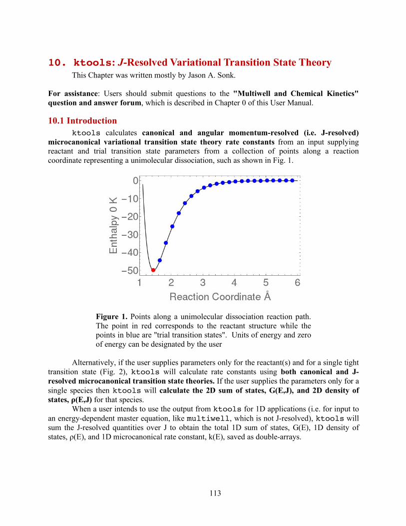
113

10. ktools: J-Resolved Variational Transition State Theory This Chapter was written mostly by Jason A. Sonk.

For assistance: Users should submit questions to the "Multiwell and Chemical Kinetics" question and answer forum, which is described in Chapter 0 of this User Manual.

10.1 Introduction ktools calculates canonical and angular momentum-resolved (i.e. J-resolved)

microcanonical variational transition state theory rate constants from an input supplying reactant and trial transition state parameters from a collection of points along a reaction coordinate representing a unimolecular dissociation, such as shown in Fig. 1.

Figure 1. Points along a unimolecular dissociation reaction path. The point in red corresponds to the reactant structure while the points in blue are "trial transition states". Units of energy and zero of energy can be designated by the user

Alternatively, if the user supplies parameters only for the reactant(s) and for a single tight

transition state (Fig. 2), ktools will calculate rate constants using both canonical and J-resolved microcanonical transition state theories. If the user supplies the parameters only for a single species then ktools will calculate the 2D sum of states, G(E,J), and 2D density of states, ρ(E,J) for that species.

When a user intends to use the output from ktools for 1D applications (i.e. for input to an energy-dependent master equation, like multiwell, which is not J-resolved), ktools will sum the J-resolved quantities over J to obtain the total 1D sum of states, G(E), 1D density of states, ρ(E), and 1D microcanonical rate constant, k(E), saved as double-arrays.

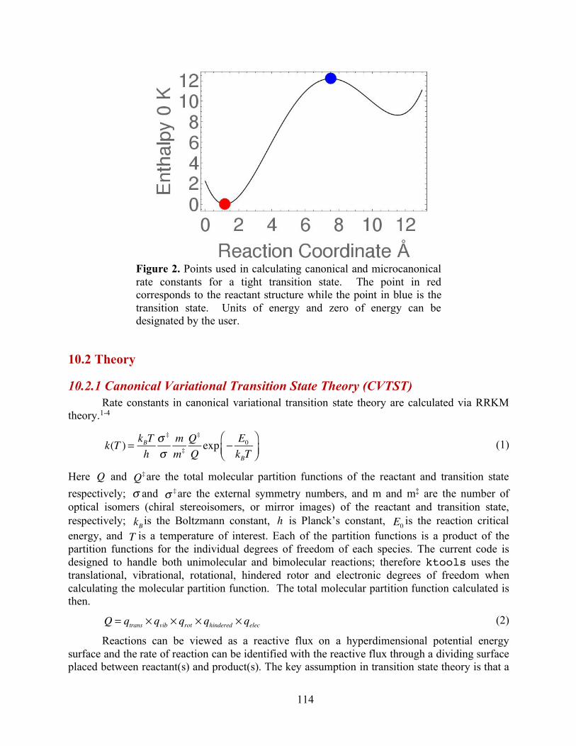
114

Figure 2. Points used in calculating canonical and microcanonical rate constants for a tight transition state. The point in red corresponds to the reactant structure while the point in blue is the transition state. Units of energy and zero of energy can be designated by the user.

10.2 Theory

10.2.1 Canonical Variational Transition State Theory (CVTST) Rate constants in canonical variational transition state theory are calculated via RRKM

theory.1-4

(1)

Here and are the total molecular partition functions of the reactant and transition state respectively; and are the external symmetry numbers, and m and m‡ are the number of optical isomers (chiral stereoisomers, or mirror images) of the reactant and transition state, respectively; is the Boltzmann constant, is Planck’s constant, is the reaction critical energy, and is a temperature of interest. Each of the partition functions is a product of the partition functions for the individual degrees of freedom of each species. The current code is designed to handle both unimolecular and bimolecular reactions; therefore ktools uses the translational, vibrational, rotational, hindered rotor and electronic degrees of freedom when calculating the molecular partition function. The total molecular partition function calculated is then.

(2)

Reactions can be viewed as a reactive flux on a hyperdimensional potential energy surface and the rate of reaction can be identified with the reactive flux through a dividing surface placed between reactant(s) and product(s). The key assumption in transition state theory is that a

k(T ) = kBTh

σ ‡

σmm‡

Q‡

Qexp − E0

kBT⎛⎝⎜

⎞⎠⎟

Q Q‡

σ σ ‡

kB h E0T

Q = qtrans × qvib × qrot × qhindered × qelec

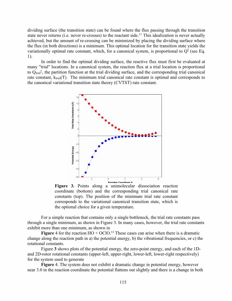
115

dividing surface (the transition state) can be found where the flux passing through the transition state never returns (i.e. never re-crosses) to the reactant side.11 This idealization is never actually achieved, but the amount of re-crossing can be minimized by placing the dividing surface where the flux (in both directions) is a minimum. This optimal location for the transition state yields the variationally optimal rate constant, which, for a canonical system, is proportional to Q‡ (see Eq. 1).

In order to find the optimal dividing surface, the reactive flux must first be evaluated at many "trial" locations. In a canonical system, the reaction flux at a trial location is proportional to Qtrial‡, the partition function at the trial dividing surface, and the corresponding trial canonical rate constant, ktrial(T). The minimum trial canonical rate constant is optimal and corresponds to the canonical variational transition state theory (CVTST) rate constant.

Figure 3. Points along a unimolecular dissociation reaction coordinate (bottom) and the corresponding trial canonical rate constants (top). The position of the minimum trial rate constant corresponds to the variational canonical transition state, which is the optional choice for a given temperature.

For a simple reaction that contains only a single bottleneck, the trial rate constants pass

through a single minimum, as shown in Figure 3. In many cases, however, the trial rate constants exhibit more than one minimum, as shown in

Figure 4 for the reaction HO + OClO.12 These cases can arise when there is a dramatic change along the reaction path in a) the potential energy, b) the vibrational frequencies, or c) the rotational constants.

Figure 3 shows plots of the potential energy, the zero-point energy, and each of the 1D- and 2D-rotor rotational constants (upper-left, upper-right, lower-left, lower-right respectively) for the system used to generate

Figure 4. The system does not exhibit a dramatic change in potential energy, however near 3.0 in the reaction coordinate the potential flattens out slightly and there is a change in both

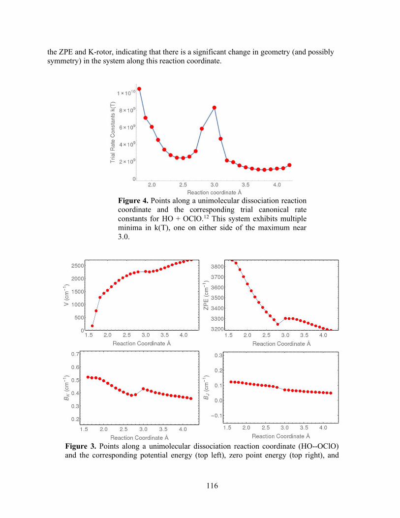
116

the ZPE and K-rotor, indicating that there is a significant change in geometry (and possibly symmetry) in the system along this reaction coordinate.

Figure 4. Points along a unimolecular dissociation reaction coordinate and the corresponding trial canonical rate constants for HO + OClO.12 This system exhibits multiple minima in k(T), one on either side of the maximum near 3.0.

Figure 3. Points along a unimolecular dissociation reaction coordinate (HO--OClO) and the corresponding potential energy (top left), zero point energy (top right), and

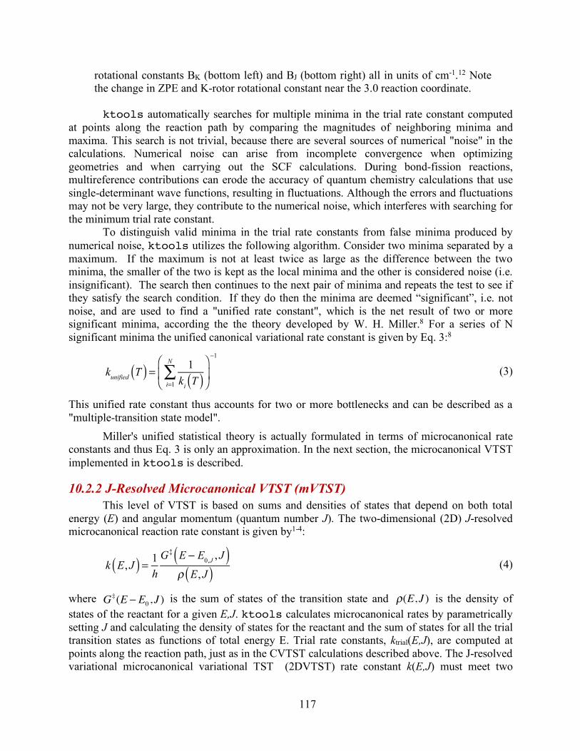
117

rotational constants BK (bottom left) and BJ (bottom right) all in units of cm-1.12 Note the change in ZPE and K-rotor rotational constant near the 3.0 reaction coordinate. ktools automatically searches for multiple minima in the trial rate constant computed

at points along the reaction path by comparing the magnitudes of neighboring minima and maxima. This search is not trivial, because there are several sources of numerical "noise" in the calculations. Numerical noise can arise from incomplete convergence when optimizing geometries and when carrying out the SCF calculations. During bond-fission reactions, multireference contributions can erode the accuracy of quantum chemistry calculations that use single-determinant wave functions, resulting in fluctuations. Although the errors and fluctuations may not be very large, they contribute to the numerical noise, which interferes with searching for the minimum trial rate constant.

To distinguish valid minima in the trial rate constants from false minima produced by numerical noise, ktools utilizes the following algorithm. Consider two minima separated by a maximum. If the maximum is not at least twice as large as the difference between the two minima, the smaller of the two is kept as the local minima and the other is considered noise (i.e. insignificant). The search then continues to the next pair of minima and repeats the test to see if they satisfy the search condition. If they do then the minima are deemed “significant”, i.e. not noise, and are used to find a "unified rate constant", which is the net result of two or more significant minima, according the the theory developed by W. H. Miller.8 For a series of N significant minima the unified canonical variational rate constant is given by Eq. 3:8

(3)

This unified rate constant thus accounts for two or more bottlenecks and can be described as a "multiple-transition state model".

Miller's unified statistical theory is actually formulated in terms of microcanonical rate constants and thus Eq. 3 is only an approximation. In the next section, the microcanonical VTST implemented in ktools is described.

10.2.2 J-Resolved Microcanonical VTST (mVTST) This level of VTST is based on sums and densities of states that depend on both total

energy (E) and angular momentum (quantum number J). The two-dimensional (2D) J-resolved microcanonical reaction rate constant is given by1-4:

(4)

where is the sum of states of the transition state and is the density of states of the reactant for a given E,J. ktools calculates microcanonical rates by parametrically setting J and calculating the density of states for the reactant and the sum of states for all the trial transition states as functions of total energy E. Trial rate constants, ktrial(E,J), are computed at points along the reaction path, just as in the CVTST calculations described above. The J-resolved variational microcanonical variational TST (2DVTST) rate constant k(E,J) must meet two

kunified T( ) = 1

ki T( )i=1

N

∑⎛

⎝⎜

⎞

⎠⎟

−1

k E, J( ) = 1

hG‡ E − E0,J , J( )

ρ E, J( )G‡(E − E0, J ) ρ(E, J )

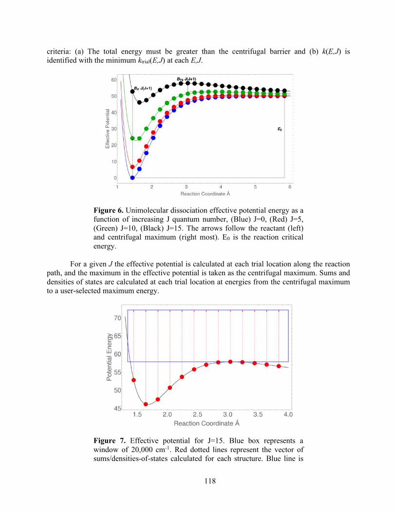
118

criteria: (a) The total energy must be greater than the centrifugal barrier and (b) k(E,J) is identified with the minimum ktrial(E,J) at each E,J.

Figure 6. Unimolecular dissociation effective potential energy as a function of increasing J quantum number, (Blue) J=0, (Red) J=5, (Green) J=10, (Black) J=15. The arrows follow the reactant (left) and centrifugal maximum (right most). E0 is the reaction critical energy.

For a given J the effective potential is calculated at each trial location along the reaction

path, and the maximum in the effective potential is taken as the centrifugal maximum. Sums and densities of states are calculated at each trial location at energies from the centrifugal maximum to a user-selected maximum energy.

Figure 7. Effective potential for J=15. Blue box represents a window of 20,000 cm-1. Red dotted lines represent the vector of sums/densities-of-states calculated for each structure. Blue line is

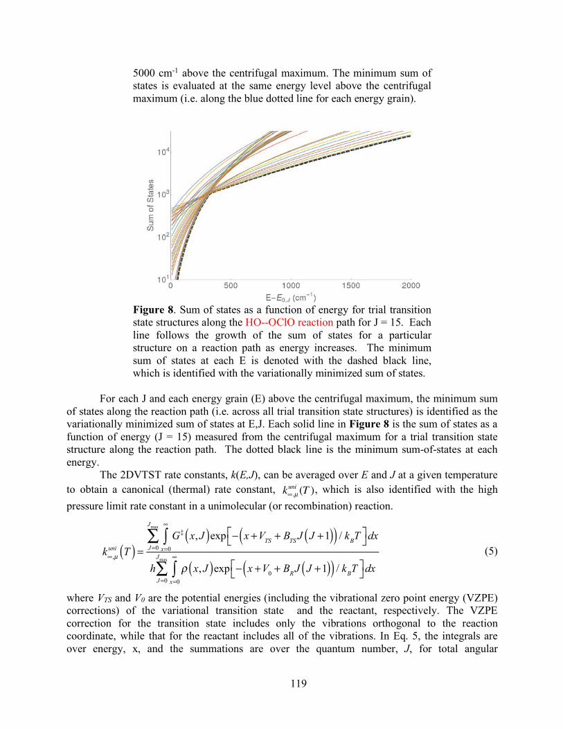
119

5000 cm-1 above the centrifugal maximum. The minimum sum of states is evaluated at the same energy level above the centrifugal maximum (i.e. along the blue dotted line for each energy grain).

Figure 8. Sum of states as a function of energy for trial transition state structures along the HO--OClO reaction path for J = 15. Each line follows the growth of the sum of states for a particular structure on a reaction path as energy increases. The minimum sum of states at each E is denoted with the dashed black line, which is identified with the variationally minimized sum of states.

For each J and each energy grain (E) above the centrifugal maximum, the minimum sum

of states along the reaction path (i.e. across all trial transition state structures) is identified as the variationally minimized sum of states at E,J. Each solid line in Figure 8 is the sum of states as a function of energy (J = 15) measured from the centrifugal maximum for a trial transition state structure along the reaction path. The dotted black line is the minimum sum-of-states at each energy.

The 2DVTST rate constants, k(E,J), can be averaged over E and J at a given temperature to obtain a canonical (thermal) rate constant, , which is also identified with the high pressure limit rate constant in a unimolecular (or recombination) reaction.

(5)

where VTS and V0 are the potential energies (including the vibrational zero point energy (VZPE) corrections) of the variational transition state and the reactant, respectively. The VZPE correction for the transition state includes only the vibrations orthogonal to the reaction coordinate, while that for the reactant includes all of the vibrations. In Eq. 5, the integrals are over energy, x, and the summations are over the quantum number, J, for total angular

k∞,µuni (T )

k∞,µuni T( ) =

G‡ x, J( )exp − x +VTS + BTS J J +1( )( ) / kBT⎡⎣

⎤⎦dx

x=0

∞

∫J=0

Jmax

∑

h ρ x, J( )exp − x +V0 + BR J J +1( )( ) / kBT⎡⎣

⎤⎦dx

x=0

∞

∫J=0

Jmax

∑

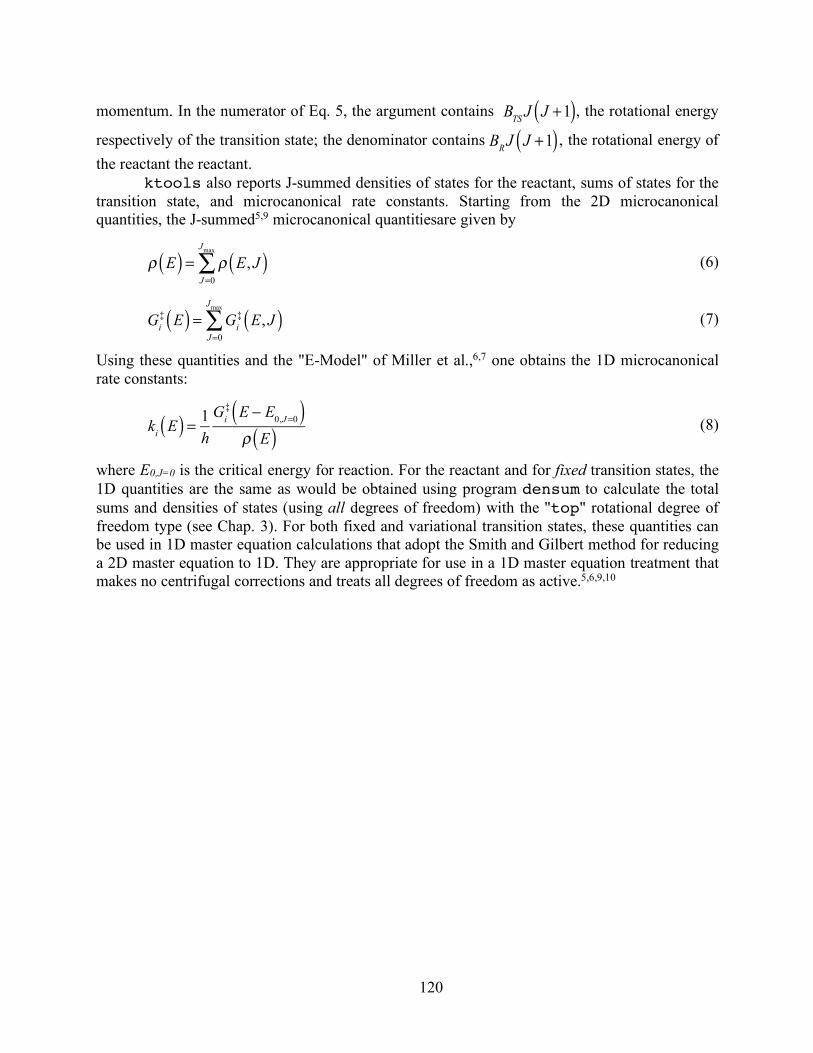
120

momentum. In the numerator of Eq. 5, the argument contains , the rotational energy

respectively of the transition state; the denominator contains , the rotational energy of the reactant the reactant.

ktools also reports J-summed densities of states for the reactant, sums of states for the transition state, and microcanonical rate constants. Starting from the 2D microcanonical quantities, the J-summed5,9 microcanonical quantitiesare given by

(6)

(7)

Using these quantities and the "E-Model" of Miller et al.,6,7 one obtains the 1D microcanonical rate constants:

(8)

where E0,J=0 is the critical energy for reaction. For the reactant and for fixed transition states, the 1D quantities are the same as would be obtained using program densum to calculate the total sums and densities of states (using all degrees of freedom) with the "top" rotational degree of freedom type (see Chap. 3). For both fixed and variational transition states, these quantities can be used in 1D master equation calculations that adopt the Smith and Gilbert method for reducing a 2D master equation to 1D. They are appropriate for use in a 1D master equation treatment that makes no centrifugal corrections and treats all degrees of freedom as active.5,6,9,10

BTS J J +1( ) BR J J +1( )

ρ E( ) = ρ E, J( )

J=0

Jmax

∑

Gi

‡ E( ) = Gi‡ E, J( )

J=0

Jmax

∑

ki E( ) = 1

hGi

‡ E − E0,J=0( )ρ E( )

121

10.3 ktools Input File The input file for a ktools calculation is similar to the input file used by program

thermo, but with several minor additions/changes. The character-based keywords do not depend on case. The code is based on the assumption that the molecular system of interest can be described with sufficient accuracy as a symmetric top (the quasi-symmetric top approximation; see Appendix B.4 of this User Manual). For that reason, the parameters for the external rotations must be specified as a “J-rotor” and “K-rotor” (corresponding respectively to the B2 and B1 rotational constants discussed in Appendix B.4).

Line 1 Title (BLANK LINES FOLLOWING TITLE ARE IGNORED) Title: 180 Character limit title to be used in output files. Line 2 Up to 20 Comment lines, each preceded by "!" (180 character limit, each

line) Line 3 Ekey, Sskey Ekey: keyword for energy units, valid options: kcal, kJ, cm-1 Sskey: keyword for standard state, not currently used (assumed to be MCC) Line 4 WhatDo WhatDo: Flag that controls writing of the large output files containing sums and

densities of states, and microcanonical rate constants ( other output files are allways generated). Valid options: savefiles generates the large output files, while any other word (e.g. nosavefiles) suppresses their output. [Note that the meaning of WhatDo was changed starting with the 2020 version of ktools.]

Line 5 Emax, Egrain Emax: Max energy to calculate sums and densities of states, in units of cm-1 Egrain: energy grain used in microcanonical TST, in units of cm-1; corresponds to Egrain1

in a double array. Line 6 Jmax, Jgrain Jmax: Max J value to calculate sums and densities of state. Jgrain: step size in J used in microcanonical TST, currently step size of 1 is

recommended. Line 7 Imax1, Isize, Emax2 These parameters describe the double arrays (generated by J-summing) for use in the multiwell master equation code (note that Egrain1 is specified on Line 4).

Imax1: Number of array elements in lower part of double array. Isize: Total number of elements in double array. Emax2: Maximum energy of double array.

122

Line 8 Nt Nt: number of temperatures to be read in Line 9 T1, T2, T3 … Tnt

T1, T2,…,Tnt: list of Nt temperatures in kelvin Line 10 RCNT, NTTS, PCNT RCNT: number of reactant molecules to read in (reactant count). Max=2 NTTS: number of trial transition states to read in PCNT: number of products to read in Default Max of RCNT+NTTS+PCNT is set to 100 Structure blocks: repeated RCNT+NTTS+PCNT times This structure of the data block for each species is slightly different than the structure

used in program thermo! Line 11.1 Reprod, molname, delh, dist reprod: species identification. Options: ctst, reac, prod molname: name of species. Used for naming relevant output files delh: enthalpy of formation at 0 K. dist: corresponding distance along reaction path, defined by the user but typically a

bond distance. This allows the canonical variational transition state theory code to report the variationally optimal transition state.

Line 11.2 Formula formula: empirical formula; used only for recombination reactions Line 11.3 Comment line A 1st comment: 150-character limit Line 11.4 Comment line B 2nd comment: 150-character limit Line 11.5 Comment line C 3rd comment: 150-character limit Line 11.6 Sym, Sopt, Nele Sym: external symmetry number; see Appendices B.4 and B.5 Sopt: number of optical isomers; see Appendix B.5 Nele: number of electronic energy levels Line 11.7 Elev, gele (Repeated Nele times) Elev: electronic energy level (lowest should be designated as Elev=0.0) Gele: electronic energy level degeneracies

123

Line 11.8 N, Vhar, Vrot N: number of degrees of freedom to read in Vhar: keyword for vibrations. Options: har Vrot: keyword for molecular internal (hra, hrb, hrc) and external rotations (kro,

jro). Options: amua for moments of inertia in units of amu Å2 gmcm for moments of inertia in units of g cm2 cm-1 for rotational constants in wavenumbers mhz for rotational constants in MHz ghz for rotational constants in GHz Repeat Line 10.9 N times, once for each degree of freedom Line 11.9 Mode(i), Idof(i), AAA(i), BBB(i), CCC(i) mode: index number for degree of freedom idof: keyword for type of degree of freedom. The separable degrees of freedom

(except for the J-rotor and K-rotor) that are recognized by ktools are defined and the data input formats are described in Chapter 3 of this User Manual. The J-rotor and K-rotor parameters used by ktools are described here:

kro: K-rotor 1-dimensional external rotation AAA = rotational moment of inertia/constant in units of Vrot BBB = rotational symmetry number CCC = rotation dimension (should always be set to 1)

jro: J-rotor 2-dimensional external rotation AAA = rotational moment of inertia/constant in units of Vrot BBB = rotational symmetry number CCC = rotation dimension (usually should be set to 2)

Line 12 (Blank Line)

124

10.4 Running ktools By default the program looks for the input file named “ktools.dat” and ktools can

be executed from the command line by simply typing “ktools”, followed by a carriage return Optionally, the user can use custom names for input files. ktools is then executed by typing “ktools filename.dat”. Where filename.dat is the filename as defined by the user. The program expects a 3-letter extension to be used in the naming of the input file name.

Comments on program execution:

A backup file (filename.bck) for the input is saved every time the code is run.

The maximum number of energy grains is limited only by the size of available computer memory (although execution speed will become very slow for extremely large calculations). For accurate canonical rate constants, Users should select emax ≥ 15×kBT ≈ 10*T cm–1 (line 5) and jmax ≥ 500 (Line 6). Typically, Egrain should be set to ~10 cm–1 and Jgrain = 1. For very low temperatures, Egrain can be reduced, but the code has not been tested below 1 cm–1.

If the maximum number of rotational states selected by the user is not large enough, execution will be terminated and an error message will suggest a larger value.

If the maximum number of rotational states selected by the user exceeds the intrinsic upper limit where Veff for the reactant is ≥Veff for all of the trial transition states, the output is automatically limited to the intrinsic limit.

The numbers of energy grains, rotational states, and the intrinsic upper limit are now reported along with the canonical rate constants (filename.canonical).

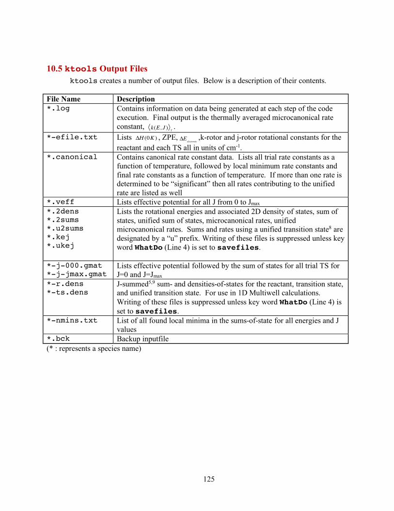
125

10.5 ktools Output Files ktools creates a number of output files. Below is a description of their contents.

File Name Description *.log Contains information on data being generated at each step of the code

execution. Final output is the thermally averaged microcanonical rate constant, .

*-efile.txt Lists , ZPE, ,k-rotor and j-rotor rotational constants for the reactant and each TS all in units of cm-1.

*.canonical Contains canonical rate constant data. Lists all trial rate constants as a function of temperature, followed by local minimum rate constants and final rate constants as a function of temperature. If more than one rate is determined to be “significant” then all rates contributing to the unified rate are listed as well

*.veff Lists effective potential for all J from 0 to Jmax *.2dens *.2sums *.u2sums *.kej *.ukej

Lists the rotational energies and associated 2D density of states, sum of states, unified sum of states, microcanonical rates, unified microcanonical rates. Sums and rates using a unified transition state8 are designated by a “u” prefix. Writing of these files is suppressed unless key word WhatDo (Line 4) is set to savefiles.

*-j-000.gmat *-j-jmax.gmat

Lists effective potential followed by the sum of states for all trial TS for J=0 and J=Jmax

*-r.dens *-ts.dens

J-summed5,9 sum- and densities-of-states for the reactant, transition state, and unified transition state. For use in 1D Multiwell calculations. Writing of these files is suppressed unless key word WhatDo (Line 4) is set to savefiles.

*-nmins.txt List of all found local minima in the sums-of-state for all energies and J values

*.bck Backup inputfile (* : represents a species name)

k(E, J ) T

ΔH (0K ) ΔEelectronic

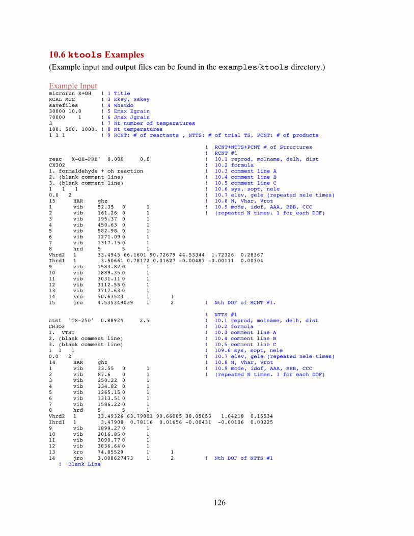
126

10.6 ktools Examples (Example input and output files can be found in the examples/ktools directory.) Example Input microrun X+OH ! 1 Title KCAL MCC ! 3 Ekey, Sskey savefiles ! 4 Whatdo 30000 10.0 ! 5 Emax Egrain 70000 1 ! 6 Jmax Jgrain 3 ! 7 Nt number of temperatures 100. 500. 1000. ! 8 Nt temperatures 1 1 1 ! 9 RCNT: # of reactants , NTTS: # of trial TS, PCNT: # of products ! RCNT+NTTS+PCNT # of Structures ! RCNT #1 reac 'X-OH-PRE' 0.000 0.0 ! 10.1 reprod, molname, delh, dist CX3O2 ! 10.2 formula 1. formaldehyde + oh reaction ! 10.3 comment line A 2. (blank comment line) ! 10.4 comment line B 3. (blank comment line) ! 10.5 comment line C 1 1 1 ! 10.6 sys, sopt, nele 0.0 2 ! 10.7 elev, gele (repeated nele times) 15 HAR ghz ! 10.8 N, Vhar, Vrot 1 vib 52.35 0 1 ! 10.9 mode, idof, AAA, BBB, CCC 2 vib 161.26 0 1 ! (repeated N times. 1 for each DOF) 3 vib 195.37 0 1 4 vib 450.63 0 1 5 vib 582.98 0 1 6 vib 1271.09 0 1 7 vib 1317.15 0 1 8 hrd 5 5 1 Vhrd2 1 33.4945 66.1601 90.72679 44.53344 1.72326 0.28367 Ihrd1 1 3.50661 0.78172 0.01627 -0.00487 -0.00111 0.00304 9 vib 1583.82 0 1 10 vib 1889.35 0 1 11 vib 3031.11 0 1 12 vib 3112.55 0 1 13 vib 3717.63 0 1 14 kro 50.63523 1 1 15 jro 4.535349039 1 2 ! Nth DOF of RCNT #1. ! NTTS #1 ctst 'TS-250' 0.88924 2.5 ! 10.1 reprod, molname, delh, dist CH3O2 ! 10.2 formula 1. VTST ! 10.3 comment line A 2. (blank comment line) ! 10.4 comment line B 3. (blank comment line) ! 10.5 comment line C 1 1 1 ! 109.6 sys, sopt, nele 0.0 2 ! 10.7 elev, gele (repeated nele times) 14 HAR ghz ! 10.8 N, Vhar, Vrot 1 vib 33.55 0 1 ! 10.9 mode, idof, AAA, BBB, CCC 2 vib 87.6 0 1 ! (repeated N times. 1 for each DOF) 3 vib 250.22 0 1 4 vib 334.82 0 1 5 vib 1265.15 0 1 6 vib 1313.51 0 1 7 vib 1586.22 0 1 8 hrd 5 5 1 Vhrd2 1 33.49326 63.79801 90.66085 38.05053 1.04218 0.15534 Ihrd1 1 3.47908 0.78116 0.01656 -0.00431 -0.00106 0.00225 9 vib 1899.27 0 1 10 vib 3016.85 0 1 11 vib 3090.77 0 1 12 vib 3836.64 0 1 13 kro 74.85529 1 1 14 jro 3.008627473 1 2 ! Nth DOF of NTTS #1 ! Blank Line

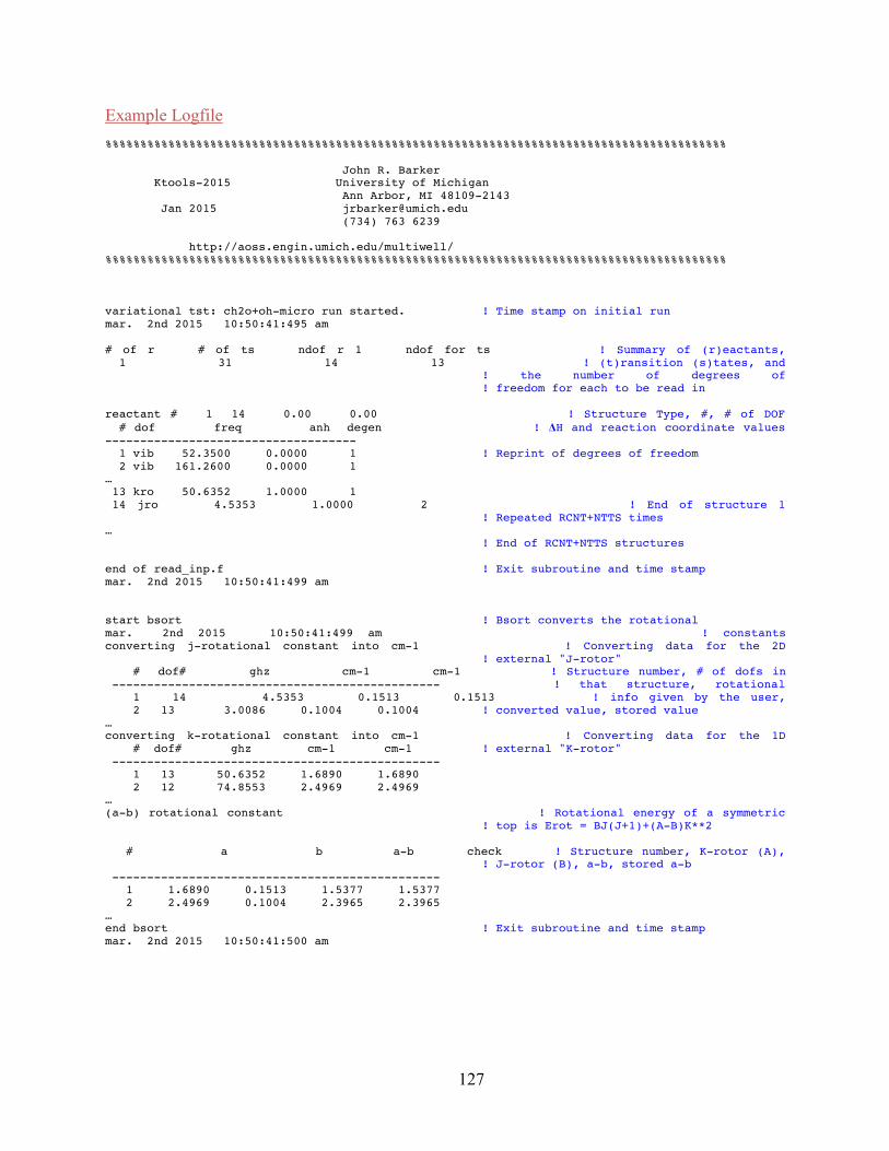
127

Example Logfile %%%%%%%%%%%%%%%%%%%%%%%%%%%%%%%%%%%%%%%%%%%%%%%%%%%%%%%%%%%%%%%%%%%%%%%%%%%%%%%%%%%%%%%%% John R. Barker Ktools-2015 University of Michigan Ann Arbor, MI 48109-2143 Jan 2015 [email protected] (734) 763 6239 http://aoss.engin.umich.edu/multiwell/ %%%%%%%%%%%%%%%%%%%%%%%%%%%%%%%%%%%%%%%%%%%%%%%%%%%%%%%%%%%%%%%%%%%%%%%%%%%%%%%%%%%%%%%%% variational tst: ch2o+oh-micro run started. ! Time stamp on initial run mar. 2nd 2015 10:50:41:495 am # of r # of ts ndof r 1 ndof for ts ! Summary of (r)eactants, 1 31 14 13 ! (t)ransition (s)tates, and ! the number of degrees of ! freedom for each to be read in reactant # 1 14 0.00 0.00 ! Structure Type, #, # of DOF # dof freq anh degen ! ΔH and reaction coordinate values ------------------------------------ 1 vib 52.3500 0.0000 1 ! Reprint of degrees of freedom 2 vib 161.2600 0.0000 1 … 13 kro 50.6352 1.0000 1 14 jro 4.5353 1.0000 2 ! End of structure 1 ! Repeated RCNT+NTTS times … ! End of RCNT+NTTS structures end of read_inp.f ! Exit subroutine and time stamp mar. 2nd 2015 10:50:41:499 am start bsort ! Bsort converts the rotational mar. 2nd 2015 10:50:41:499 am ! constants converting j-rotational constant into cm-1 ! Converting data for the 2D ! external "J-rotor" # dof# ghz cm-1 cm-1 ! Structure number, # of dofs in ----------------------------------------------- ! that structure, rotational 1 14 4.5353 0.1513 0.1513 ! info given by the user, 2 13 3.0086 0.1004 0.1004 ! converted value, stored value … converting k-rotational constant into cm-1 ! Converting data for the 1D # dof# ghz cm-1 cm-1 ! external "K-rotor" ----------------------------------------------- 1 13 50.6352 1.6890 1.6890 2 12 74.8553 2.4969 2.4969 … (a-b) rotational constant ! Rotational energy of a symmetric ! top is Erot = BJ(J+1)+(A-B)K**2 # a b a-b check ! Structure number, K-rotor (A), ! J-rotor (B), a-b, stored a-b ----------------------------------------------- 1 1.6890 0.1513 1.5377 1.5377 2 2.4969 0.1004 2.3965 2.3965 … end bsort ! Exit subroutine and time stamp mar. 2nd 2015 10:50:41:500 am

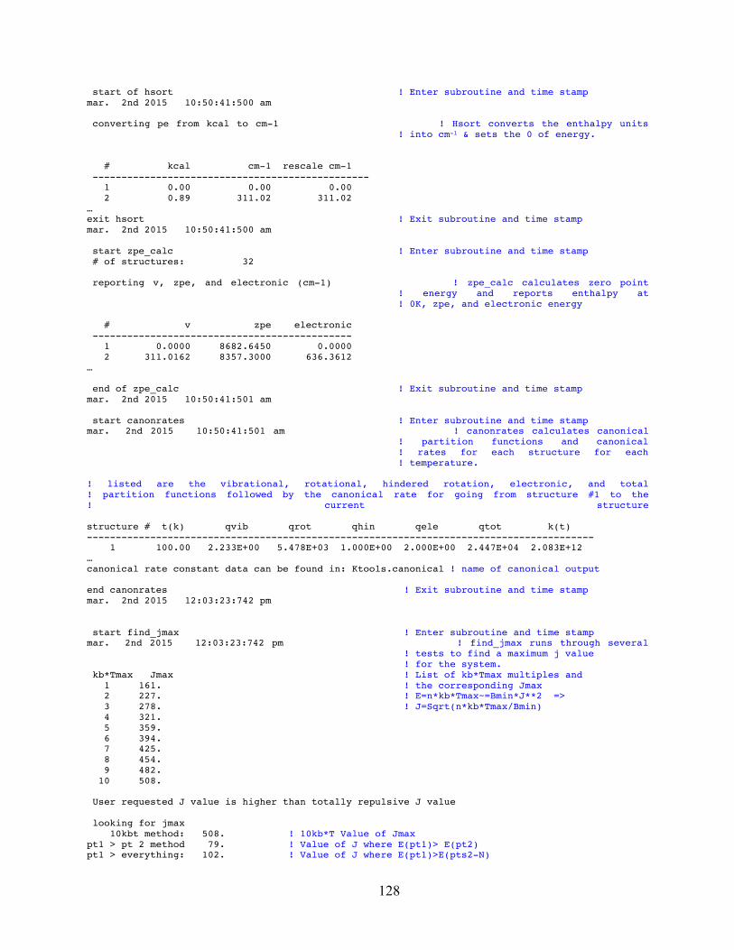
128

start of hsort ! Enter subroutine and time stamp mar. 2nd 2015 10:50:41:500 am converting pe from kcal to cm-1 ! Hsort converts the enthalpy units ! into cm-1 & sets the 0 of energy. # kcal cm-1 rescale cm-1 ------------------------------------------------ 1 0.00 0.00 0.00 2 0.89 311.02 311.02 … exit hsort ! Exit subroutine and time stamp mar. 2nd 2015 10:50:41:500 am start zpe_calc ! Enter subroutine and time stamp # of structures: 32 reporting v, zpe, and electronic (cm-1) ! zpe_calc calculates zero point ! energy and reports enthalpy at ! 0K, zpe, and electronic energy # v zpe electronic --------------------------------------------- 1 0.0000 8682.6450 0.0000 2 311.0162 8357.3000 636.3612 … end of zpe_calc ! Exit subroutine and time stamp mar. 2nd 2015 10:50:41:501 am start canonrates ! Enter subroutine and time stamp mar. 2nd 2015 10:50:41:501 am ! canonrates calculates canonical ! partition functions and canonical ! rates for each structure for each ! temperature. ! listed are the vibrational, rotational, hindered rotation, electronic, and total ! partition functions followed by the canonical rate for going from structure #1 to the ! current structure structure # t(k) qvib qrot qhin qele qtot k(t) ---------------------------------------------------------------------------------------- 1 100.00 2.233E+00 5.478E+03 1.000E+00 2.000E+00 2.447E+04 2.083E+12 … canonical rate constant data can be found in: Ktools.canonical ! name of canonical output end canonrates ! Exit subroutine and time stamp mar. 2nd 2015 12:03:23:742 pm start find_jmax ! Enter subroutine and time stamp mar. 2nd 2015 12:03:23:742 pm ! find_jmax runs through several ! tests to find a maximum j value ! for the system. kb*Tmax Jmax ! List of kb*Tmax multiples and 1 161. ! the corresponding Jmax 2 227. ! E=n*kb*Tmax~=Bmin*J**2 => 3 278. ! J=Sqrt(n*kb*Tmax/Bmin) 4 321. 5 359. 6 394. 7 425. 8 454. 9 482. 10 508. User requested J value is higher than totally repulsive J value looking for jmax 10kbt method: 508. ! 10kb*T Value of Jmax pt1 > pt 2 method 79. ! Value of J where E(pt1)> E(pt2) pt1 > everything: 102. ! Value of J where E(pt1)>E(pts2-N)

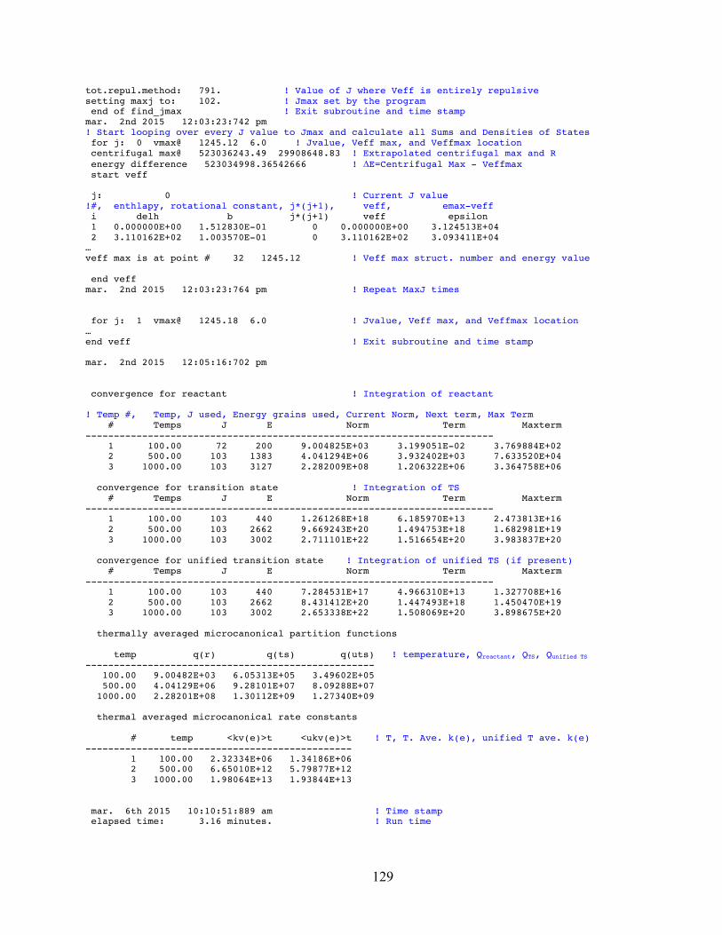
129

tot.repul.method: 791. ! Value of J where Veff is entirely repulsive setting maxj to: 102. ! Jmax set by the program end of find_jmax ! Exit subroutine and time stamp mar. 2nd 2015 12:03:23:742 pm ! Start looping over every J value to Jmax and calculate all Sums and Densities of States for j: 0 vmax@ 1245.12 6.0 ! Jvalue, Veff max, and Veffmax location centrifugal max@ 523036243.49 29908648.83 ! Extrapolated centrifugal max and R energy difference 523034998.36542666 ! ΔE=Centrifugal Max - Veffmax start veff j: 0 ! Current J value !#, enthlapy, rotational constant, j*(j+1), veff, emax-veff i delh b j*(j+1) veff epsilon 1 0.000000E+00 1.512830E-01 0 0.000000E+00 3.124513E+04 2 3.110162E+02 1.003570E-01 0 3.110162E+02 3.093411E+04 … veff max is at point # 32 1245.12 ! Veff max struct. number and energy value end veff mar. 2nd 2015 12:03:23:764 pm ! Repeat MaxJ times for j: 1 vmax@ 1245.18 6.0 ! Jvalue, Veff max, and Veffmax location … end veff ! Exit subroutine and time stamp mar. 2nd 2015 12:05:16:702 pm convergence for reactant ! Integration of reactant ! Temp #, Temp, J used, Energy grains used, Current Norm, Next term, Max Term # Temps J E Norm Term Maxterm ------------------------------------------------------------------------ 1 100.00 72 200 9.004825E+03 3.199051E-02 3.769884E+02 2 500.00 103 1383 4.041294E+06 3.932402E+03 7.633520E+04 3 1000.00 103 3127 2.282009E+08 1.206322E+06 3.364758E+06 convergence for transition state ! Integration of TS # Temps J E Norm Term Maxterm ------------------------------------------------------------------------ 1 100.00 103 440 1.261268E+18 6.185970E+13 2.473813E+16 2 500.00 103 2662 9.669243E+20 1.494753E+18 1.682981E+19 3 1000.00 103 3002 2.711101E+22 1.516654E+20 3.983837E+20 convergence for unified transition state ! Integration of unified TS (if present) # Temps J E Norm Term Maxterm ------------------------------------------------------------------------ 1 100.00 103 440 7.284531E+17 4.966310E+13 1.327708E+16 2 500.00 103 2662 8.431412E+20 1.447493E+18 1.450470E+19 3 1000.00 103 3002 2.653338E+22 1.508069E+20 3.898675E+20 thermally averaged microcanonical partition functions temp q(r) q(ts) q(uts) ! temperature, Qreactant, QTS, Qunified TS --------------------------------------------------- 100.00 9.00482E+03 6.05313E+05 3.49602E+05 500.00 4.04129E+06 9.28101E+07 8.09288E+07 1000.00 2.28201E+08 1.30112E+09 1.27340E+09 thermal averaged microcanonical rate constants # temp <kv(e)>t <ukv(e)>t ! T, T. Ave. k(e), unified T ave. k(e) ----------------------------------------------- 1 100.00 2.32334E+06 1.34186E+06 2 500.00 6.65010E+12 5.79877E+12 3 1000.00 1.98064E+13 1.93844E+13 mar. 6th 2015 10:10:51:889 am ! Time stamp elapsed time: 3.16 minutes. ! Run time

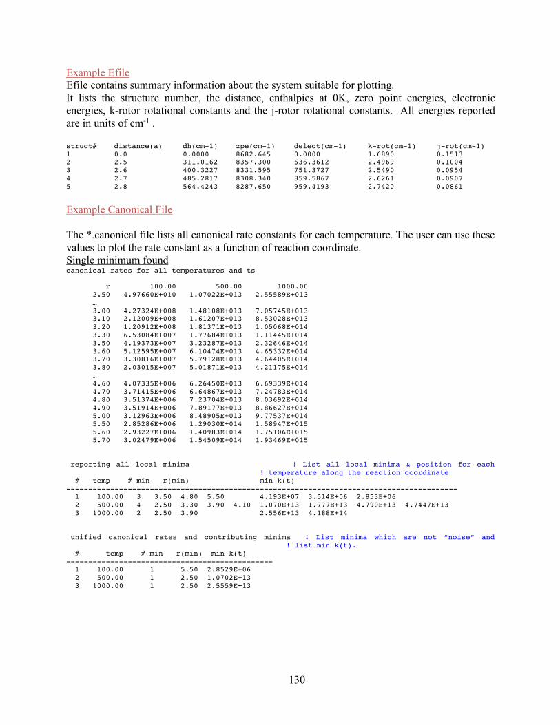
130

Example Efile Efile contains summary information about the system suitable for plotting. It lists the structure number, the distance, enthalpies at 0K, zero point energies, electronic energies, k-rotor rotational constants and the j-rotor rotational constants. All energies reported are in units of cm-1 . struct# distance(a) dh(cm-1) zpe(cm-1) delect(cm-1) k-rot(cm-1) j-rot(cm-1) 1 0.0 0.0000 8682.645 0.0000 1.6890 0.1513 2 2.5 311.0162 8357.300 636.3612 2.4969 0.1004 3 2.6 400.3227 8331.595 751.3727 2.5490 0.0954 4 2.7 485.2817 8308.340 859.5867 2.6261 0.0907 5 2.8 564.4243 8287.650 959.4193 2.7420 0.0861

Example Canonical File The *.canonical file lists all canonical rate constants for each temperature. The user can use these values to plot the rate constant as a function of reaction coordinate. Single minimum found canonical rates for all temperatures and ts r 100.00 500.00 1000.00 2.50 4.97660E+010 1.07022E+013 2.55589E+013 … 3.00 4.27324E+008 1.48108E+013 7.05745E+013 3.10 2.12009E+008 1.61207E+013 8.53028E+013 3.20 1.20912E+008 1.81371E+013 1.05068E+014 3.30 6.53084E+007 1.77684E+013 1.11445E+014 3.50 4.19373E+007 3.23287E+013 2.32646E+014 3.60 5.12595E+007 6.10474E+013 4.65332E+014 3.70 3.30816E+007 5.79128E+013 4.64405E+014 3.80 2.03015E+007 5.01871E+013 4.21175E+014 … 4.60 4.07335E+006 6.26450E+013 6.69339E+014 4.70 3.71415E+006 6.64867E+013 7.24783E+014 4.80 3.51374E+006 7.23704E+013 8.03692E+014 4.90 3.51914E+006 7.89177E+013 8.86627E+014 5.00 3.12963E+006 8.48905E+013 9.77537E+014 5.50 2.85286E+006 1.29030E+014 1.58947E+015 5.60 2.93227E+006 1.40983E+014 1.75106E+015 5.70 3.02479E+006 1.54509E+014 1.93469E+015 reporting all local minima ! List all local minima & position for each ! temperature along the reaction coordinate # temp # min r(min) min k(t) ----------------------------------------------------------------------------------------- 1 100.00 3 3.50 4.80 5.50 4.193E+07 3.514E+06 2.853E+06 2 500.00 4 2.50 3.30 3.90 4.10 1.070E+13 1.777E+13 4.790E+13 4.7447E+13 3 1000.00 2 2.50 3.90 2.556E+13 4.188E+14 unified canonical rates and contributing minima ! List minima which are not “noise” and ! list min k(t). # temp # min r(min) min k(t) ----------------------------------------------- 1 100.00 1 5.50 2.8529E+06 2 500.00 1 2.50 1.0702E+13 3 1000.00 1 2.50 2.5559E+13

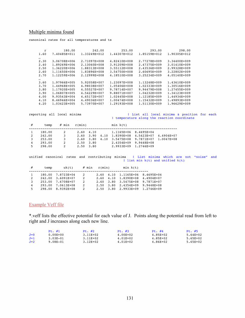
131

Multiple minima found canonical rates for all temperatures and ts r 180.00 242.00 253.00 293.00 298.00 1.60 7.40485E+011 1.33249E+012 1.44307E+012 1.85159E+012 1.90305E+012 … 2.30 3.06708E+006 2.71097E+008 4.82410E+008 2.77278E+009 3.34400E+009 2.40 1.89269E+006 2.13060E+008 3.91209E+008 2.47375E+009 3.01410E+009 2.50 1.36220E+006 1.88313E+008 3.55112E+008 2.43536E+009 2.99328E+009 2.60 1.11650E+006 1.83896E+008 3.54750E+008 2.60695E+009 3.22802E+009 2.70 1.12259E+006 2.12999E+008 4.18510E+008 3.25234E+009 4.05140E+009 … 3.60 1.97966E+005 5.92058E+007 1.23097E+008 1.13248E+009 1.43610E+009 3.70 1.44968E+005 4.98038E+007 1.05406E+008 1.02333E+009 1.30516E+009 3.80 1.17920E+005 4.55527E+007 9.78714E+007 9.94479E+008 1.27455E+009 3.90 1.06807E+005 4.54229E+007 9.88071E+007 1.04232E+009 1.34123E+009 4.00 9.93543E+004 4.65172E+007 1.02445E+008 1.12185E+009 1.44934E+009 4.10 8.46946E+004 4.49036E+007 1.00474E+008 1.15432E+009 1.49893E+009 4.20 1.03423E+005 5.73970E+007 1.29193E+008 1.51130E+009 1.96629E+009 reporting all local minima ! List all local minima & position for each ! temperature along the reaction coordinate # temp # min r(min) min k(t) ----------------------------------------------------------------------------- 1 180.00 2 2.60 4.10 1.1165E+06 8.4695E+04 2 242.00 3 2.60 3.90 4.10 1.8390E+08 4.5423E+07 4.4904E+07 3 253.00 3 2.60 3.80 4.10 3.5475E+08 9.7871E+07 1.0047E+08 4 293.00 2 2.50 3.80 2.4354E+09 9.9448E+08 5 298.00 2 2.50 3.80 2.9933E+09 1.2746E+09 unified canonical rates and contributing minima ! List minima which are not “noise” and ! list min k(t) and unified k(t) # temp uk(t) # min r(min) min k(t) -------------------------------------------------------------- 1 180.00 7.8723E+04 2 2.60 4.10 1.1165E+06 8.4695E+04 2 242.00 3.6091E+07 2 2.60 4.10 1.8390E+08 4.4904E+07 3 253.00 7.6708E+07 2 2.60 3.80 3.5475E+08 9.7871E+07 4 293.00 7.0613E+08 2 2.50 3.80 2.4354E+09 9.9448E+08 5 298.00 8.9392E+08 2 2.50 3.80 2.9933E+09 1.2746E+09

Example Veff file *.veff lists the effective potential for each value of J. Points along the potential read from left to right and J increases along each new line. Pt. #1 Pt. #2 Pt. #3 Pt. #4 Pt. #5 J=0 0.00E+00 3.11E+02 4.00E+02 4.85E+02 5.64E+02 J=1 3.03E-01 3.11E+02 4.01E+02 4.85E+02 5.65E+02 J=2 9.08E-01 3.12E+02 4.01E+02 4.86E+02 5.65E+02

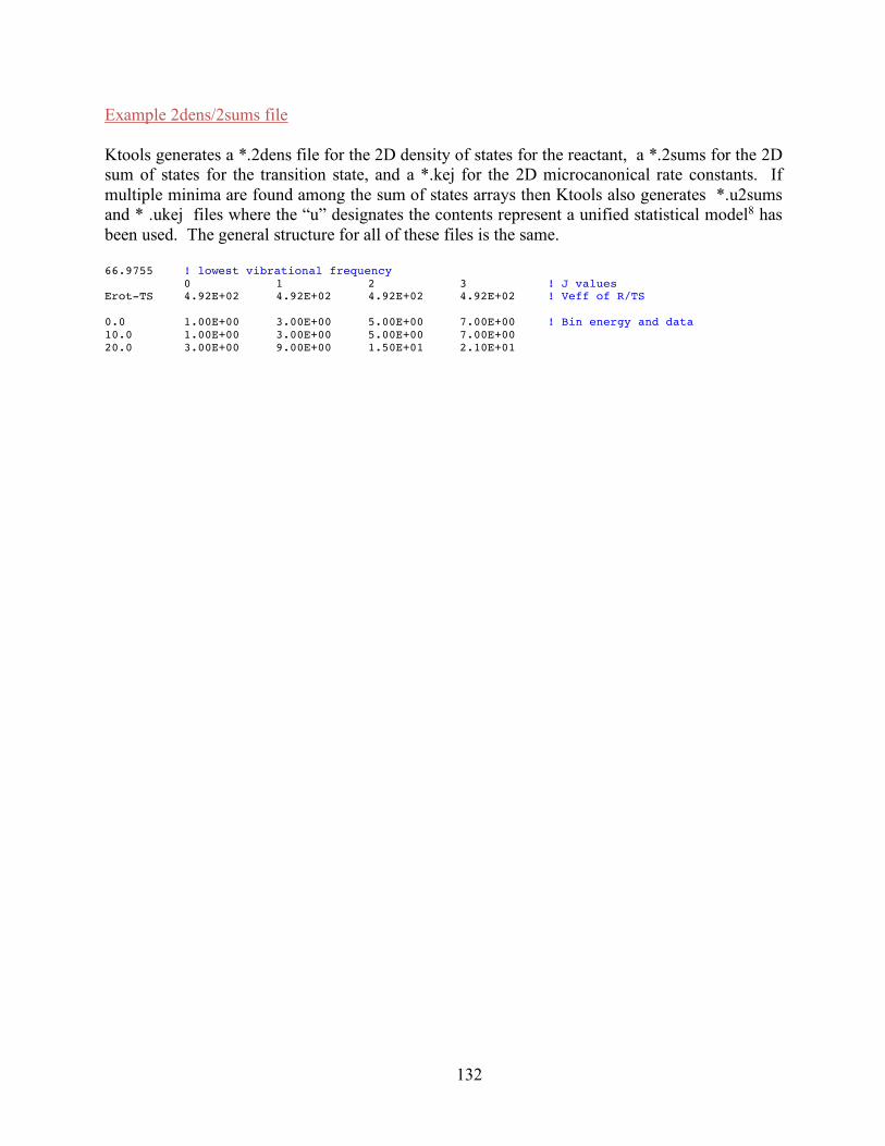
132

Example 2dens/2sums file Ktools generates a *.2dens file for the 2D density of states for the reactant, a *.2sums for the 2D sum of states for the transition state, and a *.kej for the 2D microcanonical rate constants. If multiple minima are found among the sum of states arrays then Ktools also generates *.u2sums and * .ukej files where the “u” designates the contents represent a unified statistical model8 has been used. The general structure for all of these files is the same. 66.9755 ! lowest vibrational frequency 0 1 2 3 ! J values Erot-TS 4.92E+02 4.92E+02 4.92E+02 4.92E+02 ! Veff of R/TS 0.0 1.00E+00 3.00E+00 5.00E+00 7.00E+00 ! Bin energy and data 10.0 1.00E+00 3.00E+00 5.00E+00 7.00E+00 20.0 3.00E+00 9.00E+00 1.50E+01 2.10E+01

133

References

(1) Baer, T.; Hase, W. L. Unimolecular Reaction Dynamics. Theory and Experiments; Oxford University Press: New York, 1996.

(2) Forst, W. Unimolecular Reactions. A Concise Introduction; Cambridge University Press: Cambridge, 2003.

(3) Gilbert, R. G.; Smith, S. C. Theory of Unimolecular and Recombination Reactions; Blackwell Scientific Publications: Oxford, 1990.


(5) Klippenstein, S. J.; Harding, L. B. A direct transition state theory based study of methyl radical recombination kinetics. Journal of Physical Chemistry A 1999, 103, 9388-9398.


(7) Miller, J. A.; Klippenstein, S. J.; Raffy, C. Solution of some one- and two-dimensional master equation models for thermal dissociation: The dissociation of methane in the low pressure limit. JPCA 2002, 106, 4904-4913.

(8) Miller, W. H. Unified statistical model for "complex" and "direct" reaction mechanisms. J. Chem. Phys. 1976, 65, 2216-2223; https://doi.org/10.1063/1.433379.



(11) Truhlar, D. G.; Garrett, B. C. Variational Transition State Theory. Ann. Rev. Phys. Chem. 1984, 35, 159-189.

(12) Yang, L.; Sonk, J. A.; Barker, J. R. HO + OClO Reaction System: Featuring a Barrierless Entrance Channel with Two Transition States. J. Phys. Chem. A 2015, 119, 5723–5731; DOI: 10.1021/acs.jpca.5b03487.

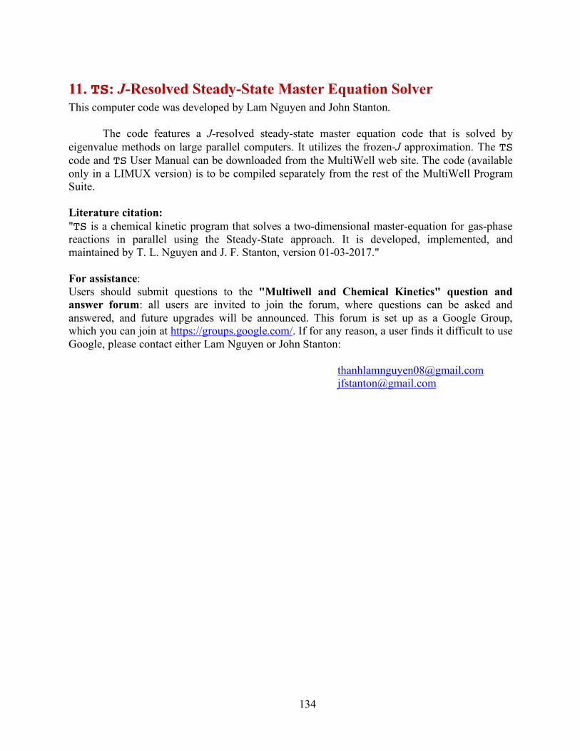
134

11. TS: J-Resolved Steady-State Master Equation Solver This computer code was developed by Lam Nguyen and John Stanton.

The code features a J-resolved steady-state master equation code that is solved by

eigenvalue methods on large parallel computers. It utilizes the frozen-J approximation. The TS code and TS User Manual can be downloaded from the MultiWell web site. The code (available only in a LIMUX version) is to be compiled separately from the rest of the MultiWell Program Suite.

Literature citation: "TS is a chemical kinetic program that solves a two-dimensional master-equation for gas-phase reactions in parallel using the Steady-State approach. It is developed, implemented, and maintained by T. L. Nguyen and J. F. Stanton, version 01-03-2017."

For assistance: Users should submit questions to the "Multiwell and Chemical Kinetics" question and answer forum: all users are invited to join the forum, where questions can be asked and answered, and future upgrades will be announced. This forum is set up as a Google Group, which you can join at https://groups.google.com/. If for any reason, a user finds it difficult to use Google, please contact either Lam Nguyen or John Stanton:

[email protected] [email protected]

135

Appendix A. Theoretical Basis Much of this Appendix is based on an expanded and corrected version of the paper

originally published in the International Journal of Chemical Kinetics: J.R. Barker, Multiple-well, multiple-reaction-path unimolecular reaction systems. I. MultiWell computer program suite. Int. J. Chem. Kinetics, 33, 232-45 (2001). For a recent review of Monte Carlo stochastic methods for simulationg master equations, see Barker.6

A.1. Introduction Here, the theoretical basis for MultiWell is summarized. Inevitably, various

approximations and assumptions must be adopted due to computational limitations and to the absence of physico-chemical knowledge. The numerical approximations are described so that program users can better assess MultiWell's limitations and strengths. The principal assumptions made in formulating the master equation are reviewed.

In the next section, the master equation is described formally. In subsequent sections, the stochastic methodology is described along with a brief discussion of some of the merits and limitations of the hybrid master equation approach relative to other methods. Methods for computing microcanonical unimolecular reaction rates and energy transfer step sizes are described, followed by a description of various initial conditions that can be selected as options. Finally, the calculation input and output are outlined.

A.2. The Active Energy Master Equation The current version of MultiWell is based on the one-dimensional master equation,26 in

which the active (randomizable) internal energy is modeled, but it is planned that future extensions will explicitly include angular momentum (the two-dimensional master equation17,22,25,27,29-32,35,36). The master equation provides the fundamental theoretical basis for modeling systems in which both energy transfer and chemical reaction can occur.4,11,12,14,28 It is comprised of a set of coupled integro-differential equations that describe the rates of production and loss of chemical species at specified energies.

A.2.1 Internal Energy and Active Degrees of Freedom Unless slow intramolecular vibrational energy redistribution (IVR) is specified, the

internal energy E is always assumed to be fully randomized among the active degrees of freedom. The internal energy for a particular species (stable molecule or transition state) includes the energy (measured from the zero point energy; see Figure 0) that resides in the internal modes (vibrations, torsions, and internal rotations) and an active external rotation. Nonlinear polyatomic species have three external rotational degrees of freedom characterized by moments of inertia IA, IB, and IC. The usual pragmatic approach11,12 is to assume the molecule can be approximated as a symmetric top with two of the moments of inertia equal to one another (IB = IC), producing a degenerate two-dimensional external rotation. The third external rotor is associated with the symmetric top figure axis and is sometimes termed the K-rotor. The K-rotor is assumed to exchange energy freely with the other internal degrees of freedom, while the degenerate two-dimensional external rotation is assumed to be inactive.3,11,12,14,28 See Appendix B.4 of this Manual for more discussion. (More sophisticated treatments of rotations can be utilized in the

136

present version of MultiWell by calculating specific rate constants (k(E)) externally and then providing them in data files read by MultiWell.)

Figure 0. Energy schematic. The active energy E is measured from the zero point energy of the reactant well. The critical energy E0 is the zero point energy difference between the transition state and the reactant well.

A.2.2 Sums and Densities of States The MultiWell suite of computer codes includes DenSum, which utilizes the Stein-

Rabinovitch34 version of the Beyer-Swinehart algorithm9 for exact counts of states for species comprised of separable degrees of freedom. The present version of DenSum can accommodate harmonic oscillators, Morse oscillators, and free rotors. The K-rotor is included with the internal degrees of freedom when calculating the sums and densities of states. There are two options for the treatment of rotations. The usual option is to use the convolution method developed by Astholz et al.,1 which is computationally efficient and accurate for rotors with small rotational constants. The second method is to use exact counts of rotational states. The second method is preferred if the rotational constant is larger than ~1 cm-1. DenSum produces an output file that is subsequently used as an input file by MultiWell. The inactive two-dimensional external rotation is specified in the general MultiWell data file.

Hindered Internal Rotations In the MultiWell Program Suite, torsional modes are assumed to be separable from other

motions (i.e. translations, vibrations, external rotations and other internal rotations) and are treated as one-dimensional quantum hindered internal rotations. The Schrödinger equation for such 1-D torsional motions is solved as described in the Technical Notes (see Appendix B).

137

The 1-D torsion coordinate is defined as χ, the torsional dihedral angle (0≤χ<2p). Users must supply the potential energy V(χ) and the torsion rotational constant function Bhr(χ) (or the corresponding moment of inertia function I(χ)). Potential energies V(χ) and molecular geometries can be computed at discrete values of χ by using any of the many available quantum chemistry codes, such as Gaussian,13 Molpro,38 or CFour.33 The results for V(χ) can be fitted to a suitable truncated Fourier series. Program lamm, a module in the MultiWell Program Suite, is intended to help users compute Bhr(χ), based on the output from quantum chemistry programs (see Chapter 8 of this manual).

A.2.3 Master Equation for the Vibrational Quasi-Continuum Because of the difficulties encountered in solving the 2-D master equation, it is usually

reduced to 1-D by making simplifying assumptions, and then solving numerically by one of the standard methods.4,5,20,21,24 However, Marcus showed that the microcanonical RRKM specific rate constant depends on the active energy E, i.e. the energy not constrained by conservation of angular momentum. Thus angular momentum has an effect that must be taken into account for accurate results. The first approach to this problem also originated with Marcus,18 who invoked the concept of adiabatic rotation to make "centrifugal corrections". Marcus' approach has been reviewed by Waage and Rabinovitch37 and is found in standard monographs.12,14,16 In this approach, the RRKM specific rate constant k(Et,J), which is written as depending on total energy Et and the angular momentum quantum number J is reduced to an approximate k(E) (at a given temperature), where E is the active energy of the reactant: all explicit reference to angular momentum quantum number J has been removed from the 2DME, which has thus been reduced to a 1DME. This approach is outlined in the following.

At high vibrational energies, a quasicontinuum of vibrational states exists and intramolecular vibrational redistribution (IVR) is rapid. Experiments show that IVR is slow at low energy, exhibits multiple time scales, and becomes rapid at energies where the vibrational state density is of the order of 102–103 states/cm-1.23 At these state densities, some vibrational states overlap significantly within their natural widths as governed by infrared spontaneous emission rates. At state densities greater than ~107 states/cm-1, most states are overlapped within their natural widths. The onset of "rapid" IVR is a convenient marker for the onset of the vibrational quasicontinuum. However, this criterion leaves some uncertainty because IVR exhibits multiple time constants and thus some modes remain isolated even at higher vibrational state densities.23

A shorter version of the following derivation of centrifugal corrections has been reported elsewhere.39

In the vibrational quasicontinuum, individual quantum states cannot be resolved and the master equation can be written as a function of either of two equivalent sets of independent variables: Et,J or E,J. In terms of active energy E and angular momentum quantum number J, it takes the following form 12,14,20,24:

(2.3-1)

dN ( ′E , ′J ,t)dt

= ′F ′E , ′J ,t( )+ R ′E , ′J ; E, J( ) N E, J ;t( )dE0

∞

∫J∑

− R E, J ; ′E , ′J( ) N ′E , ′J ,t( )dE0

∞

∫J∑ − ki ′E , ′J( )N ′E , ′J ,t( )

i=1

channels

∑

138

where the primed E' and J' refer to the current state and the unprimed quantities refer to a different state of the excited species, which is undergoing reaction. In Eq. 2.3-1, N(E',J',t)dE' is the concentration of a chemical species with active energy in the range E' to E'+dE'; R(E,J;E',J') is the (pseudo-first-order) rate coefficient for collisional energy transfer from initial energy E' to energy E and quantum number J' to J; F'(E',J',t)dE' is a source term (e.g. thermal, chemical, or photo activation, or isomerization); and ki(E',J') is the unimolecular reaction rate constant for molecules at energy E' and rotational quantum number J' reacting via the ith reaction channel.

To reduce the 2DME to a 1DME, we first assume that the rotational population distribution describing the adiabatic rotations is always Boltzmann:

(2.3-2a)

where gJ = 2J+1 for a 2-D symmetric top (which is typically assumed; see Appendix B.4 of this Manual) and other forms for 1-D and spherical tops; the rotational energy EJ and the rotational partition function QJ for the adiabatic rotor(s) are given by Eq. 2.3-2b and 2.3-2c, respectively:

(2.3-2b)

(2.3-2c)

The constant B is the rotational constant. By using these expressions, the concentrations can be written as

(2.3-3)

In the same spirit, we assume the source function produces the same rotational distribution:

(2.3-4)

Although recent trajectory calculations show that the assumption is probably not accurate,8) we follow Smith and Gilbert31 and Miller et al.21 in adopting the pragmatic assumption that the collision rates in Eq. 1 can be written in a separable form:

(2.3-5)

where R(E,E') has no dependence on angular momentum and can be expressed as the product of the total vibrationally inelastic collision frequency (w) multiplied by the "collision step-size distribution", P(E,E'), which expresses the probability that a molecule initially in the energy range from E' to E'+dE' will undergo an inelastic transition to the energy range E to E+dE:

, (2.3-6a)

(2.3-6b)

The first factor on the right hand side of Equation (2.3-6a), the integral over the rates of all inelastic transitions from initial energy E' can be identified with the frequency of inelastic

Pe J( ) = QJ−1gJ exp −EJ / kBT( )

EJ = BJ J +1( )

QJ = gJ exp −EJ / kBT( )

J∑

N E, J ,t( ) = N E,t( )Pe J( )

′F ′E , ′J ,t( ) = F ′E ,t( )Pe J '( )

R E, J ; ′E , ′J( ) = R E, ′E( )Pe J( )

R(E, ′E )dE= R(E, ′E )dE0

∞

∫R(E, ′E )dE

R(E, ′E )dE0

∞

∫

⎧

⎨⎪⎪

⎩⎪⎪

⎫

⎬⎪⎪

⎭⎪⎪

=ω P(E, ′E )dE

139

collisions, w, which may depend on the initial active energy E'. Usually, the collision frequency is calculated from the expression w = kc[M], where kc is the bimolecular rate constant for inelastic collisions and [M] is bath gas concentration. The second factor (in curly brackets) on the right hand side of Equation (2.3-6a) is P(E,E')dE. It is important to emphasize that the factorization of R(E,E') in Equation (2.3-6) is merely for convenience and that kc and P(E,E') never occur independently of one another. Furthermore, P(E,E') is only a proper probability density function when w is exactly equal to the inelastic collision rate constant. With this assumption, P(E,E') is normalized:

(2.3-7)

Note that collision step-size distributions for activating and deactivating collisions are connected via detailed balance:

, (2.3-8)

where r(E) is the density of states at active energy E, Ttrans is the translational temperature, and kB is the Boltzmann constant. The relationships among P(E,E'), kc, and the normalization integral are further discussed below.

Using these definitions, we obtain

(2.3-9)

Smith and Gilbert showed that the master equation can be solved approximately when using this separable form. In MultiWell, this separable form is adopted pragmatically in order to obtain a semi-analytical solution to the master equation. (Miller and coworkers have further generalized the function postulated by Smith and Gilbert,31 and the details may be found in their papers.20,21)

After combining Eq. 2.3-1-9, we obtain

(2.3-10)

In this expression, the sums over J are equal to unity because Pe(J) is normalized. Every term contains the factor Pe(J'). By summing every term in Eq. 2.3-6 over J' and noting that the sum equals unity in each term except the last, we obtain

(2.3-11a)

where <ki(E')>J is the RRKM specific rate constant, averaged over the rotational energy distribution:

P(E, ′E )dE

0

∞

∫ = 1

P(E, ′E )P( ′E , E)

= ρ(E)ρ( ′E )

exp − E − ′EkBTtrans

⎧⎨⎩⎪

⎫⎬⎭⎪

R E, J ; ′E , ′J( ) =ωP E, ′E( )Pe J( )

dN ( ′E ,t)dt

Pe ′J( ) = F ′E ,t( )Pe ′J( ) + Pe J( )ωPe ′J( ) P ′E ; E( ) N E;t( )dE0

∞

∫J∑

− N ′E ,t( )Pe ′J( ) Pe J( )ω P E; ′E( ) dE0

∞

∫J∑ − N ′E ,t( )Pe ′J( ) ki ′E , ′J( )

i=1

channels

∑

dN ( ′E ,t)dt

= F ′E ,t( )+ω P ′E ; E( ) N E,t( )− P E; ′E( ) N ′E ,t( )⎡⎣ ⎤⎦dE0

∞

∫

− N ′E ,t( ) ki ′E( )J

i=1

channels

∑

140

(2.3-11b)

The upper limit of the summation (J'max) in Eq. 2.3-11b corresponds to the largest angular momentum quantum number for which the well still exists. Eq. 2.3-11 summarizes the general form of the 1-D master equation treated by MultiWell.

The averaging of ki(E',J') over the rotational energy distribution may be carried out as follows, using the variables defined in Fig. 2.3-1. The RRKM specific rate constant for a specific J' can be written18

(2.3-12)

where L‡ is the reaction path degeneracy, h is Planck's constant, G‡(E+,J') is the sum of states of the transition state as a function of the active energy E+ in the transition state, and ρ(E',J') is the density of "vibrational" states of the reactant when the rotational quantum number is J'. The various energies are related as follows (see Fig. 2.3-1):

(2.3-13a)

or

(2.3-13b)

where EJ and EJ+ are the energies of the adiabatic rotations in the reactant and in the transition state, respectively, and ∆EJ = EJ+-EJ. The rotational energies are given by Eq. 2.3-2b and by the analogous equation:

(2.3-14)

Using these relationships, ki(E',J') can be written

(2.3-15)

From Eqs. 2.3-2b and 2.3-14 it is apparent that EJ = (B/B+)EJ+, and ∆EJ can be written as a function of EJ+ alone: ∆EJ = (1−B/B+)EJ+.

For reactions involving bond fission, the rotational constant B+ for a rigid rotor transition state is smaller than that for the reactant and ∆EJ < 0. As the angular momentum quantum number J' increases, the quantity (E0 - ∆EJ) approaches zero. In other words, the reactant well and the effective critical energy for reaction both vanish when J' is large enough: J'max is the largest value of J' for which the well still exists. For J' > J'max, k(E',J') is not defined. When B+ ≤ B for rigid rotors, J'max = ∞.

The rate constant must now be averaged over the rotational population distribution:

(2.3-16a)

From the definition of ∆EJ, this expression can also be written

ki ′E( )

J= Pe ′J( )ki ′E , ′J( )

′J =0

′Jmax

∑

k ′E , ′J( ) = L‡

hG‡ E+ , ′J( )ρ ′E , ′J( )

′E + EJ = E+ + E0 + E+J

′E = E+ + E0 + ΔEJ

EJ+ = B+J J +1( )

k ′E , ′J( ) = L‡

hG‡ ′E − E0 − ΔEJ( )

ρ ′E , ′J( )

k ′E , ′J( )

J= QJ

−1 k ′E , ′J( )gJ′J =0

′Jmax

∑ exp −EJ / kBT( )

141

(2.3-16b)

Equations 2.3-16a and 2.3-12b are suitable for directly averaging over the rotational quantum number. Care must be taken however, because the rate constant is only defined at energies E' ≥ (E0+∆EJ). Because ∆EJ ≤ 0, the reaction threshold may be significantly lower in energy than E0, the critical energy for J = 0.

The ad hoc approximate functions postulated by Smith and Gilbert31 and by Miller and coworkers20,21 are almost certainly not accurate.8 Thus we feel that elaborate treatments cannot be justified and have instead adopted the following pragmatic approach.

The active degrees of freedom may include one or more external rotations, which, to a good approximation, may be treated as separable (see Appendix B.4). Typically, for a prolate symmetric top, the K-rotor is regarded as active. For a rigid rotor, the K quantum number is a "good" quantum number and is restricted to the range from −J to +J. However, a highly excited molecule is hardly rigid and K is not conserved, although it may exhibit a "propensity" to be conserved for some period of time. As a result, it is commonly assumed that the K-rotor of a non-rigid top can exchange energy freely with the internal degrees of freedom: i.e. the K-rotor is usually assumed to be an active degree of freedom.

It is common practice to allow K to vary freely, except for conservation of energy, and treat the K-rotor as just one more separable degree of freedom when computing densities of states.11,12,16,28 In fact, treating the K-rotor in this way may be more accurate than restricting K to the range from −J to +J.2 (This separable-rotors approximation10 is discussed in Appendix B.4.) However, there always exist 2J'+1 states with the same value of J', even for a completely asymmetric top. Thus neglecting the restriction on K has the effect of increasing the density and sum of states slightly, but this error is insignificant except for molecules with small rotational constants at very low temperatures.

Here, it is pragmatically assumed that the K-rotor is active and the K quantum number has no restrictions other than conservation of energy. As a result, the approximate density of states of the reactant molecule has no explicit dependence on the J quantum number: ρ(E',J') is replaced by ρ(E') in Eq. 2.3-16 and the average specific rate constant can be written

(2.3-17a)

where the averaged sum of states is given by

(2.3-17b)

where J'max is the largest value of J' for which k(E',J') is defined. Another pragmatic approximation is useful. Marcus showed that by substituting an

average value <∆EJ> = (1−B/B+)<EJ+> in place of ∆EJ in Eq. 2.3-13, a useful approximate expression is obtained,18 which does not retain any explicit dependence on the rotational state J':

(2.3-18)

k ′E , ′J( )

J= QJ

−1 k ′E , ′J( )gJ′J =0

′Jmax

∑ exp − EJ+ − ΔEJ( ) / kBT⎡

⎣⎤⎦

k ′E , ′J( )

J=

L‡ G‡ ′E − E0 − ΔEJ( )J

hρ ′E( )

G‡ ′E − E0 − ΔEJ( )

J= 1

QJ

G‡ ′E − E0 − ΔEJ( )gJ exp −EJ / kBT( )′J =0

′Jmax

∑

ka ′E( ) = L‡

hG‡ ′E − E0 − ΔEJ( )

ρ ′E( )

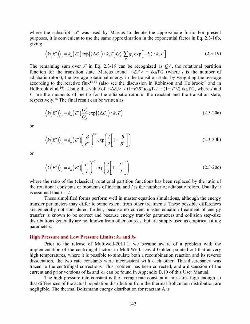
142

where the subscript "a" was used by Marcus to denote the approximate form. For present purposes, it is convenient to use the same approximation in the exponential factor in Eq. 2.3-16b, giving

(2.3-19)

The remaining sum over J' in Eq. 2.3-19 can be recognized as QJ+, the rotational partition function for the transition state. Marcus found <EJ+> = lkBT/2 (where l is the number of adiabatic rotors), the average rotational energy in the transition state, by weighting the average according to the reactive flux18,19 (also see the discussion in Robinson and Holbrook28 and in Holbrook et al.16). Using this value of <∆EJ> ≈ (1−B/B+)lkBT/2 = (1− I+/I) lkBT/2, where I and I+ are the moments of inertia for the adiabatic rotor in the reactant and the transition state, respectively.18 The final result can be written as

(2.3-20a)

or

(2.3-20b)

or

(2.3-20c)

where the ratio of the (classical) rotational partition functions has been replaced by the ratio of the rotational constants or moments of inertia, and l is the number of adiabatic rotors. Usually it is assumed that l = 2.

These simplified forms perform well in master equation simulations, although the energy transfer parameters may differ to some extent from other treatments. These possible differences are generally not considered further, because no current master equation treatment of energy transfer is known to be correct and because energy transfer parameters and collision step-size distributions generally are not known from other sources, but are simply used as empirical fitting parameters.

High Pressure and Low Pressure Limits: k∞ and k0 Prior to the release of Multiwell-2011.1, we became aware of a problem with the

implementation of the centrifugal factors in MultiWell. David Golden pointed out that at very high temperatures, where it is possible to simulate both a recombination reaction and its reverse dissociation, the two rate constants were inconsistent with each other. This discrepancy was traced to the centrifugal corrections. This problem has been corrected, and a discussion of the current and prior versions of k0 and k∞ can be found in Appendix B.10 of this User Manual.

The high pressure rate constant is the average rate constant at pressures high enough so that differences of the actual population distribution from the thermal Boltzmann distribution are negligible. The thermal Boltzmann energy distribution for reactant A is

k ′E( )

J= ka ′E( )exp ΔEJ / kBT( )QJ

−1 gJ′J∑ exp −EJ

+ / kBT⎡⎣ ⎤⎦

k ′E( )

J= ka ′E( )QJ

+

QJ

exp ΔEJ / kBT( )

k ′E( )

J= ka ′E( ) B

B+

⎛⎝⎜

⎞⎠⎟

l /2

expl2

1− BB+

⎡

⎣⎢

⎤

⎦⎥

⎛⎝⎜

⎞⎠⎟

k ′E( )

J= ka ′E( ) I +

I⎛⎝⎜

⎞⎠⎟

l /2

expl2

1− I +

I⎡

⎣⎢

⎤

⎦⎥

⎛

⎝⎜⎞

⎠⎟

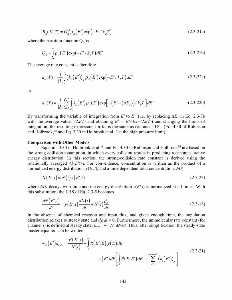
143

(2.3-21a)

where the partition function QA is

(2.3-21b)

The average rate constant is therefore

(2.3-22a)

or

(2.3-22b)

By transforming the variable of integration from E' to E+ (i.e. by replacing ∆EJ in Eq. 2.3-7b with the average value, <∆EJ> and obtaining E+ = E'−E0−<∆EJ>) and changing the limits of integration, the resulting expression for k∞ is the same as canonical TST (Eq. 4.30 of Robinson and Holbrook,28 and Eq. 3.30 in Holbrook et al.16 at the high pressure limit). Comparison with Other Models

Equation 3.30 in Holbrook et al.16 and Eq. 4.30 in Robinson and Holbrook28 are based on the strong collision assumption, in which every collision results in producing a canonical active energy distribution. In this section, the strong-collision rate constant is derived using the rotationally averaged <k(E')>J. For convenience, concentration is written as the product of a normalized energy distribution, y(E',t), and a time-dependent total concentration, N(t):

(2.3-23)

where N(t) decays with time and the energy distribution y(E',t) is normalized at all times. With this substitution, the LHS of Eq. 2.3-5 becomes

(2.3-18)

In the absence of chemical reaction and input flux, and given enough time, the population distribution relaxes to steady state and dy/dt = 0. Furthermore, the unimolecular rate constant (for channel i) is defined at steady state: kuni,i = −N-1dN/dt. Thus, after simplification the steady-state master equation can be written

(2.3-21)

BA( ′E ,T ) = QA−1ρA ′E( )exp − ′E / kBT( )

QA = ρA ′E( )exp − ′E / kBT( )d ′E

0

∞

∫

k∞(T ) = 1

QA

ka ′E( )JρA ′E( )exp − ′E / kBT( )d ′E

ε0′

∞

∫

k∞(T ) = 1

QA

QJ+

QJ

ka ′E( )ρA ′E( )exp − ′E − ΔEJ( ) / kBT⎡⎣

⎤⎦d ′E

ε0′

∞

∫

N ′E ,t( ) = N t( ) y ′E ,t( )

dN ′E ,t( )dt

= y ′E ,t( ) dN t( )dt

+ N t( ) dydt

− y ′E( )kuni,i =F ′E ,t( )

N t( ) + R ′E ; E( ) y E( )dE0

∞

∫

− y ′E( )dE R E; ′E( )dE0

∞

∫ + ki ′E( )J

i=1

channels

∑⎡

⎣⎢⎢

⎤

⎦⎥⎥

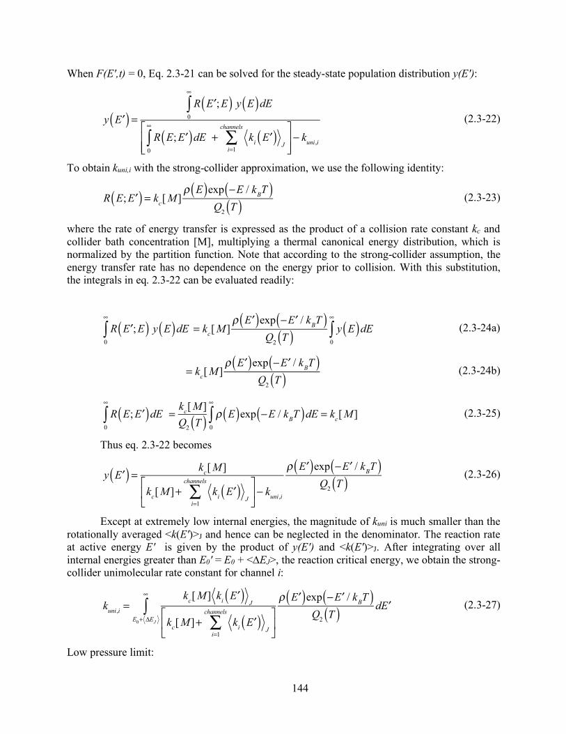
144

When F(E',t) = 0, Eq. 2.3-21 can be solved for the steady-state population distribution y(E'):

(2.3-22)

To obtain kuni,i with the strong-collider approximation, we use the following identity:

(2.3-23)

where the rate of energy transfer is expressed as the product of a collision rate constant kc and collider bath concentration [M], multiplying a thermal canonical energy distribution, which is normalized by the partition function. Note that according to the strong-collider assumption, the energy transfer rate has no dependence on the energy prior to collision. With this substitution, the integrals in eq. 2.3-22 can be evaluated readily:

(2.3-24a)

(2.3-24b)

(2.3-25)

Thus eq. 2.3-22 becomes

(2.3-26)

Except at extremely low internal energies, the magnitude of kuni is much smaller than the rotationally averaged <k(E')>J and hence can be neglected in the denominator. The reaction rate at active energy E' is given by the product of y(E') and <k(E')>J. After integrating over all internal energies greater than E0' = E0 + <∆EJ>, the reaction critical energy, we obtain the strong-collider unimolecular rate constant for channel i:

(2.3-27)

Low pressure limit:

y ′E( ) =R ′E ; E( ) y E( )dE

0

∞

∫

R E; ′E( )dE0

∞

∫ + ki ′E( )J

i=1

channels

∑⎡

⎣⎢⎢

⎤

⎦⎥⎥− kuni,i

R E; ′E( ) = kc[M ]

ρ E( )exp −E / kBT( )Q2 T( )

R ′E ; E( ) y E( )dE

0

∞

∫ = kc[M ]ρ ′E( )exp − ′E / kBT( )

Q2 T( ) y E( )dE0

∞

∫

= kc[M ]

ρ ′E( )exp − ′E / kBT( )Q2 T( )

R E; ′E( )dE

0

∞

∫ =kc[M ]Q2 T( ) ρ E( )exp −E / kBT( )dE

0

∞

∫ = kc[M ]

y ′E( ) = kc[M ]

kc[M ]+ ki ′E( )J

i=1

channels

∑⎡

⎣⎢

⎤

⎦⎥ − kuni,i

ρ ′E( )exp − ′E / kBT( )Q2 T( )

kuni,i =kc[M ] ki ′E( )

J

kc[M ]+ ki ′E( )J

i=1

channels

∑⎡

⎣⎢

⎤

⎦⎥

ρ ′E( )exp − ′E / kBT( )Q2 T( ) d ′E

E0+ ΔEJ

∞

∫

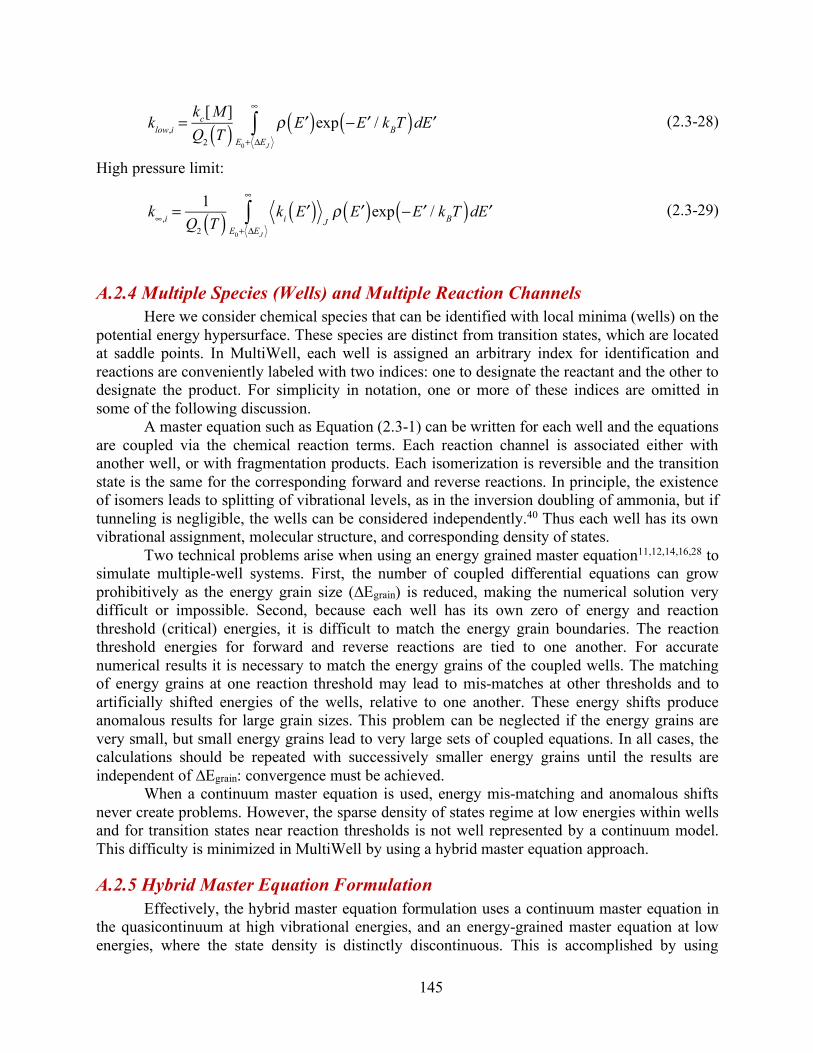
145

(2.3-28)

High pressure limit:

(2.3-29)

A.2.4 Multiple Species (Wells) and Multiple Reaction Channels Here we consider chemical species that can be identified with local minima (wells) on the

potential energy hypersurface. These species are distinct from transition states, which are located at saddle points. In MultiWell, each well is assigned an arbitrary index for identification and reactions are conveniently labeled with two indices: one to designate the reactant and the other to designate the product. For simplicity in notation, one or more of these indices are omitted in some of the following discussion.

A master equation such as Equation (2.3-1) can be written for each well and the equations are coupled via the chemical reaction terms. Each reaction channel is associated either with another well, or with fragmentation products. Each isomerization is reversible and the transition state is the same for the corresponding forward and reverse reactions. In principle, the existence of isomers leads to splitting of vibrational levels, as in the inversion doubling of ammonia, but if tunneling is negligible, the wells can be considered independently.40 Thus each well has its own vibrational assignment, molecular structure, and corresponding density of states.

Two technical problems arise when using an energy grained master equation11,12,14,16,28 to simulate multiple-well systems. First, the number of coupled differential equations can grow prohibitively as the energy grain size (∆Egrain) is reduced, making the numerical solution very difficult or impossible. Second, because each well has its own zero of energy and reaction threshold (critical) energies, it is difficult to match the energy grain boundaries. The reaction threshold energies for forward and reverse reactions are tied to one another. For accurate numerical results it is necessary to match the energy grains of the coupled wells. The matching of energy grains at one reaction threshold may lead to mis-matches at other thresholds and to artificially shifted energies of the wells, relative to one another. These energy shifts produce anomalous results for large grain sizes. This problem can be neglected if the energy grains are very small, but small energy grains lead to very large sets of coupled equations. In all cases, the calculations should be repeated with successively smaller energy grains until the results are independent of ∆Egrain: convergence must be achieved.

When a continuum master equation is used, energy mis-matching and anomalous shifts never create problems. However, the sparse density of states regime at low energies within wells and for transition states near reaction thresholds is not well represented by a continuum model. This difficulty is minimized in MultiWell by using a hybrid master equation approach.

A.2.5 Hybrid Master Equation Formulation Effectively, the hybrid master equation formulation uses a continuum master equation in

the quasicontinuum at high vibrational energies, and an energy-grained master equation at low energies, where the state density is distinctly discontinuous. This is accomplished by using

klow,i =

kc[M ]Q2 T( ) ρ ′E( )exp − ′E / kBT( )d ′E

E0+ ΔEJ

∞

∫

k∞,i =

1Q2 T( ) ki ′E( )

Jρ ′E( )exp − ′E / kBT( )d ′E

E0+ ΔEJ

∞

∫

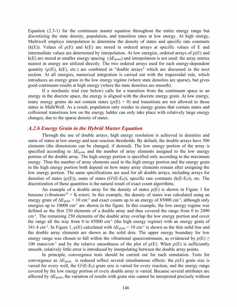
146

Equation (2.3-1) for the continuum master equation throughout the entire energy range but discretizing the state density, population, and transition rates at low energy. At high energy, Multiwell employs interpolation to determine the density of states and specific rate constants (k(E)). Values of r(E) and k(E) are stored in ordered arrays at specific values of E and intermediate values are determined by interpolation. At low energies, ordered arrays of r(E) and k(E) are stored at smaller energy spacing (∆Egrain) and interpolation is not used: the array entries nearest in energy are utilized directly. The two ordered arrays used for each energy-dependent quantity (r(E), k(E), etc.) are combined in "double arrays" which are discussed in the next section. At all energies, numerical integration is carried out with the trapezoidal rule, which introduces an energy grain in the low energy regime (where state densities are sparse), but gives good continuum results at high energy (where the state densities are smooth).

If a stochastic trial (see below) calls for a transition from the continuum space to an energy in the discrete space, the energy is aligned with the discrete energy grain. At low energy, many energy grains do not contain states (r(E) = 0) and transitions are not allowed to those states in MultiWell. As a result, population only resides in energy grains that contain states and collisional transitions low on the energy ladder can only take place with relatively large energy changes, due to the sparse density of states.

A.2.6 Energy Grain in the Hybrid Master Equation Through the use of double arrays, high energy resolution is achieved in densities and

sums of states at low energy and near reaction thresholds. By default, the double arrays have 500 elements (the dimensions can be changed, if desired). The low energy portion of the array is specified according to ∆Egrain and the number of array elements assigned to the low energy portion of the double array. The high energy portion is specified only according to the maximum energy. Thus the number of array elements used in the high energy portion and the energy grain in the high energy portion both depend on how many array elements remain after assigning the low energy portion. The same specifications are used for all double arrays, including arrays for densities of states (r(E)), sums of states (G‡(E-E0)), specific rate constants (k(E-E0)), etc. The discretization of these quantities is the natural result of exact count algorithms.

An example of a double array for the density of states r(E) is shown in Figure 1 for benzene (vibrations15 + K-rotor). In this example, the density of states was calculated using an energy grain of ∆Egrain = 10 cm-1 and exact counts up to an energy of 85000 cm-1, although only energies up to 10000 cm-1 are shown in the figure. In this example, the low energy regime was defined as the first 250 elements of a double array and thus covered the range from 0 to 2490 cm-1. The remaining 250 elements of the double array overlap the low energy portion and cover the range all the way from 0 to 85000 cm-1 (the high energy regime) with an energy grain of 341.4 cm-1. In Figure 1, r(E) calculated with ∆Egrain = 10 cm-1 is shown as the thin solid line and the double array elements are shown as the solid dots. The upper energy boundary for low energy range was chosen to fall within the vibrational quasicontinuum, as evidenced by r(E) ≥ 100 states/cm-1 and by the relative smoothness of the plot of r(E). When r(E) is sufficiently smooth, relatively little error is introduced by interpolating between the double array points.

In principle, convergence tests should be carried out for each simulation. Tests for convergence as ∆Egrain is reduced reflect several simultaneous effects: the r(E) grain size is varied for every well, the G‡(E-E0) grain size is varied for every reaction, and the energy range covered by the low energy portion of every double array is varied. Because several attributes are affected by ∆Egrain, the variation of results with grain size cannot be interpreted precisely without

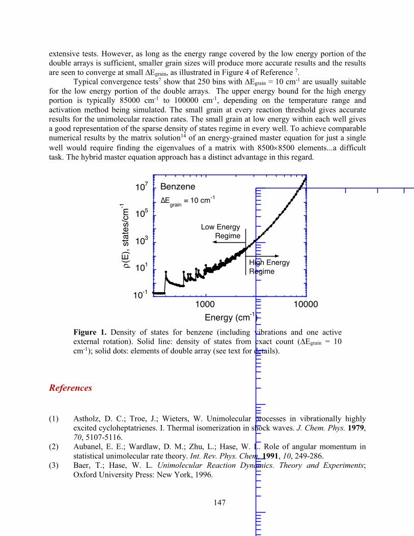
147

extensive tests. However, as long as the energy range covered by the low energy portion of the double arrays is sufficient, smaller grain sizes will produce more accurate results and the results are seen to converge at small ∆Egrain, as illustrated in Figure 4 of Reference 7.

Typical convergence tests7 show that 250 bins with ∆Egrain = 10 cm-1 are usually suitable for the low energy portion of the double arrays. The upper energy bound for the high energy portion is typically 85000 cm-1 to 100000 cm-1, depending on the temperature range and activation method being simulated. The small grain at every reaction threshold gives accurate results for the unimolecular reaction rates. The small grain at low energy within each well gives a good representation of the sparse density of states regime in every well. To achieve comparable numerical results by the matrix solution14 of an energy-grained master equation for just a single well would require finding the eigenvalues of a matrix with 8500´8500 elements...a difficult task. The hybrid master equation approach has a distinct advantage in this regard.

Figure 1. Density of states for benzene (including vibrations and one active external rotation). Solid line: density of states from exact count (∆Egrain = 10 cm-1); solid dots: elements of double array (see text for details).

References

(1) Astholz, D. C.; Troe, J.; Wieters, W. Unimolecular processes in vibrationally highly excited cycloheptatrienes. I. Thermal isomerization in shock waves. J. Chem. Phys. 1979, 70, 5107-5116.

(2) Aubanel, E. E.; Wardlaw, D. M.; Zhu, L.; Hase, W. L. Role of angular momentum in statistical unimolecular rate theory. Int. Rev. Phys. Chem. 1991, 10, 249-286.


10-1

101

103

105

107

1000 10000

ρ(E)

, sta

tes/

cm-1

Energy (cm-1)

Benzene∆Egrain = 10 cm-1

High EnergyRegime

Low EnergyRegime

148


(5) Barker, J. R. Multiple-well, multiple-path unimolecular reaction systems. I. MultiWell computer program suite. Int. J. Chem. Kinet. 2001, 33, 232-245; https://doi.org/10.1002/kin.1017.

(6) Barker, J. R. Monte Carlo stochastic simulation of the master equation for unimolecular reaction systems. In Unimolecular Kinetics. Parts 2 and 3: Collisional Energy Transfer and The Master Equation; Robertson, S. H., Ed.; Elsevier, 2019; Vol. 43; pp 409-463.


(8) Barker, J. R.; Weston, R. E., Jr. Collisional Energy Transfer Probability Densities P(E,J;E',J') for Monatomics Colliding with Large Molecules. J. Phys. Chem. A 2010, 114, 10619–10633; 10.1021/jp106443d.


(10) Current, J. H.; Rabinovitch, B. S. Decomposition of Chemically Activated Ethyl-d3 Radicals. Primary Intramolecular Kinetic Isotope Effect in a Nonequilibrium System. J. Chem. Phys. 1963, 38, 783-795.


Cambridge, 2003. (13) Frisch, M. J.; Trucks, G. W.; Schlegel, H. B.; Scuseria, G. E.; Robb, M. A.; Cheeseman,

J. R.; Scalmani, G.; Barone, V.; Mennucci, B.; Petersson, G. A.; Nakatsuji, H.; Caricato, M.; Li, X.; Hratchian, H. P.; Izmaylov, A. F.; Bloino, J.; Zheng, G.; Sonnenberg, J. L.; Hada, M.; Ehara, M.; Toyota, K.; Fukuda, R.; Hasegawa, J.; Ishida, M.; Nakajima, T.; Honda, Y.; Kitao, O.; Nakai, H.; Vreven, T.; J. A. Montgomery, J.; Peralta, J. E.; Ogliaro, F.; Bearpark, M.; Heyd, J. J.; Brothers, E.; Kudin, K. N.; Staroverov, V. N.; Kobayashi, R.; Normand, J.; Raghavachari, K.; Rendell, A.; Burant, J. C.; Iyengar, S. S.; Tomasi, J.; Cossi, M.; Rega, N.; Millam, J. M.; Klene, M.; Knox, J. E.; Cross, J. B.; Bakken, V.; Adamo, C.; Jaramillo, J.; Gomperts, R.; Stratmann, R. E.; Yazyev, O.; Austin, A. J.; Cammi, R.; Pomelli, C.; Ochterski, J. W.; Martin, R. L.; Morokuma, K.; Zakrzewski, V. G.; Voth, G. A.; Salvador, P.; Dannenberg, J. J.; Dapprich, S.; Daniels, A. D.; Farkas, O.; Foresman, J. B.; Ortiz, J. V.; Cioslowski, J.; Fox, D. J. Gaussian 09, Revision A.1; Revision A.1 ed.; Gaussian, Inc.: Wallingford CT, 2009.


(15) Goodman, L.; Ozkabak, A. G.; Thakur, S. N. A benchmark vibrational potential surface: ground state benzene. J. Phys. Chem. 1991, 95, 9044.


(17) Jeffrey, S. J.; Gates, K. E.; Smith, S. C. Full iterative solution of the two-dimensional master equation for thermal unimolecular reactions. J. Phys. Chem. 1996, 100, 7090-7096.

(18) Marcus, R. A. Dissociation and isomerization of vibrationally excited species. III. J. Chem. Phys. 1965, 43, 2658-2661.

149

(19) Marcus, R. A. Erratum: Dissociation and Isomerization of Vibrationally Excited Species [J. Chem. Phys. 43,2658 (1965)]. J. Chem. Phys. 1970, 52, 1018.


(21) Miller, J. A.; Klippenstein, S. J.; Raffy, C. Solution of some one- and two-dimensional master equation models for thermal dissociation: The dissociation of methane in the low pressure limit. JPCA 2002, 106, 4904-4913.

(22) Penner, A. P.; Forst, W. Transfer of vibrational-rotational energy in thermal reactions: application to polyatomics. Chemical Physics 1976, 13, 51-64.

(23) Perry, D. S. Time scales and mechanisms of intramolecular energy redistribution. In Highly Excited States: Relaxation, Reaction, and Structure; Mullin, A., Schatz, G. C., Eds.; American Chemical Society: Washington DC, 1997; Vol. 678; pp 70-80.

(24) Pilling, M. J.; Robertson, S. H. Master equation models for chemical reactions of importance in combustion. Annual Review of Physical Chemistry 2003, 54, 245-275.

(25) Press, W. H.; Teukolsky, S. A.; Vetterling, W. T.; Flannery, B. P. Numerical Recipes in FORTRAN. The Art of Scientific Computing, 2 ed.; Cambridge University Press: Cambridge, 1992.

(26) Robertson, S. H. Foundations of the master equation. In Unimolecular Kinetics: Parts 2 and 3: Collisional Energy Transfer and the Master Equation; Robertson, S. H., Ed.; Elsevier, 2019; Vol. 43; pp 299-361.

(27) Robertson, S. H.; Shushin, A. I.; Wardlaw, D. M. Reduction of the two dimensional master equation to a Smolouchowsky type differential equation with application to CH4 –> CH3 + H. J. Chem. Phys. 1993, 98, 8673-8679.

(28) Robinson, P. J.; Holbrook, K. A. Unimolecular Reactions; Wiley-Interscience: London; New York, 1972.

(29) Smith, S. C.; Frankcombe, T. J. Numerical Methods. In Unimolecular Kinetics: Parts 2 and 3: Collisional Energy Transfer and the Master Equation; Robertson, S. H., Ed.; Elsevier, 2019; Vol. 43; pp 363-408.



(32) Smith, S. C.; McEwan, M. J.; Gilbert, R. G. The pressure dependence of ion-molecule association rate coefficients. Journal of Chemical Physics 1989, 90, 1630-1640.

(33) Stanton, J. F.; Gauss, J.; Harding, M. E.; Szalay, P. G.; Auer, w. c. f. A. A.; Bartlett, R. J.; Benedikt, U.; Berger, C.; Bernholdt, D. E.; Bomble, Y. J.; Christiansen, O.; Heckert, M.; Heun, O.; Huber, C.; Jagan, T.-C.; Jonsson, D.; Jusélius, J.; Klein, K.; Lauderdale, W. J.; Matthews, D. A.; Metzroth, T.; O'Neill, D. P.; Price, D. R.; Prochnow, E.; Ruud, K.; Schiffmann, F.; Stopkowicz, S.; Vázquez, J.; Wang, F.; Watts, J. D. and the integral packages MOLECULE (J. Almlöf and P.R. Taylor); PROPS (P.R. Taylor); ABACUS (T. Helgaker, H.J. Aa. Jensen, P. Jørgensen, and J. Olsen); and ECP routines by A. V. Mitin and C. van Wüllen. CFOUR, a quantum chemical program package (www.cfour.de/), 2009.


150

(35) Troe, J. Theory of thermal unimolecular reactions at low pressures. I. Solution of the Master Equation. Journal of Chemical Physics 1977, 66, 4745-4757.

(36) Venkatesh, P. K.; Dean, A. M.; Cohen, M. H.; Carr, R. W. Master equation analysis of intermolecular energy transfer in multiple-well, multiple-channel unimolecular reactions. I. Basic Theory. Journal of Chemical Physics 1997, 107, 8904-8916.

(37) Waage, E. V.; Rabinovitch, B. S. Centrifugal effects in reaction rate theory. Chemical Reviews 1970, 70, 377-387.

(38) Werner, H.-J.; Knowles, P. J.; Lindh, R.; Manby, F. R.; Schütz, M.; Celani, P.; Korona, T.; Rauhut, G.; Amos, R. D.; Bernhardsson, A.; Berning, A.; Cooper, D. L.; Deegan, M. J. O.; Dobbyn, A. J.; Eckert, F.; Hampel, C.; Hetzer, G.; Lloyd, A. W.; McNicholas, S. J.; W. Meyer, W.; Mura, M. E.; Nicklass, A.; Palmieri, P.; Pitzer, R.; Schumann, U.; Stoll, H.; Stone, A. J.; Tarroni, R.; Thorsteinsson, T. MOLPRO version 2006.1 (a package of ab initio programs); version 2006.1 ed.; see http://www.molpro.net., 2006.

(39) Weston, R. E., Jr.; Nguyen, T. L.; Stanton, J. F.; Barker, J. R. HO + CO Reaction Rates and H/D Kinetic Isotope Effects: Master Equation Models with ab Initio SCTST Rate Constants. J. Phys. Chem. A 2013, 117, 821-835; http://dx.doi.org/10.1021/jp311928w,.

(40) Wilson, E. B., Jr.; Decius, J. C.; Cross, P. C. Molecular Vibrations. The Theory of Infrared and Raman Vibrational Spectra; McGraw-Hill Book Company, Inc.: New York, 1955.

A.3. Stochastic Method

A.3.1 Gillespie's (Exact) Stochastic Simulation Algorithm Gillespie showed that a stochastic method gives the exact solution to a set of ordinary

differential equations in the limit of an infinite number of stochastic trials.2,4 The algorithm has been described in the context of chemical kinetics.1,3,5 If a Markovian system is in a given state and can make transitions to other states via a set of transition rate coefficients, then for a given step in a stochastic simulation, Gillespie's algorithm gives a prescription for a) finding the duration of the time step and b) selecting the transition from among the choices. This algorithm is repeated step-by-step as long as desired and as long as transitions are possible.

Gillespie's method can be applied to both linear and non-linear systems.3 Equation (2.3-1) is linear in y(E,t), which leads to a particularly convenient result which is described below. If Equation (1) contained non-linear terms to describe energy pooling, for example, the terms would contain factors such as the product y(E,t)ý(E',t). To solve this system numerically requires using an energy-grained master equation with a swarm of stochastic trials and storing an evolving vector of populations as a function of energy. Here, the number of stochastic trials can be identified with a number of pseudo molecules that initially are placed in a set of energy grains. At each time step, a pseudo molecule is moved from one energy grain to another as described by Gillespie and the swarm of pseudo molecules maps out the evolving energy distribution. This approach has been used by Veerecken et al.10,11 to simulate unimolecular and recombination reactions and it can in principle be extended to non-linear systems. The difficulties in this approach are associated with the energy-grained master equation (see above) and with the requirement for storage of the entire vector of y(E,t) at every time step. Given the current availability of inexpensive computer memory, the latter is not a serious limitation for single-well reaction systems. When several wells are involved, the bookkeeping is cumbersome.

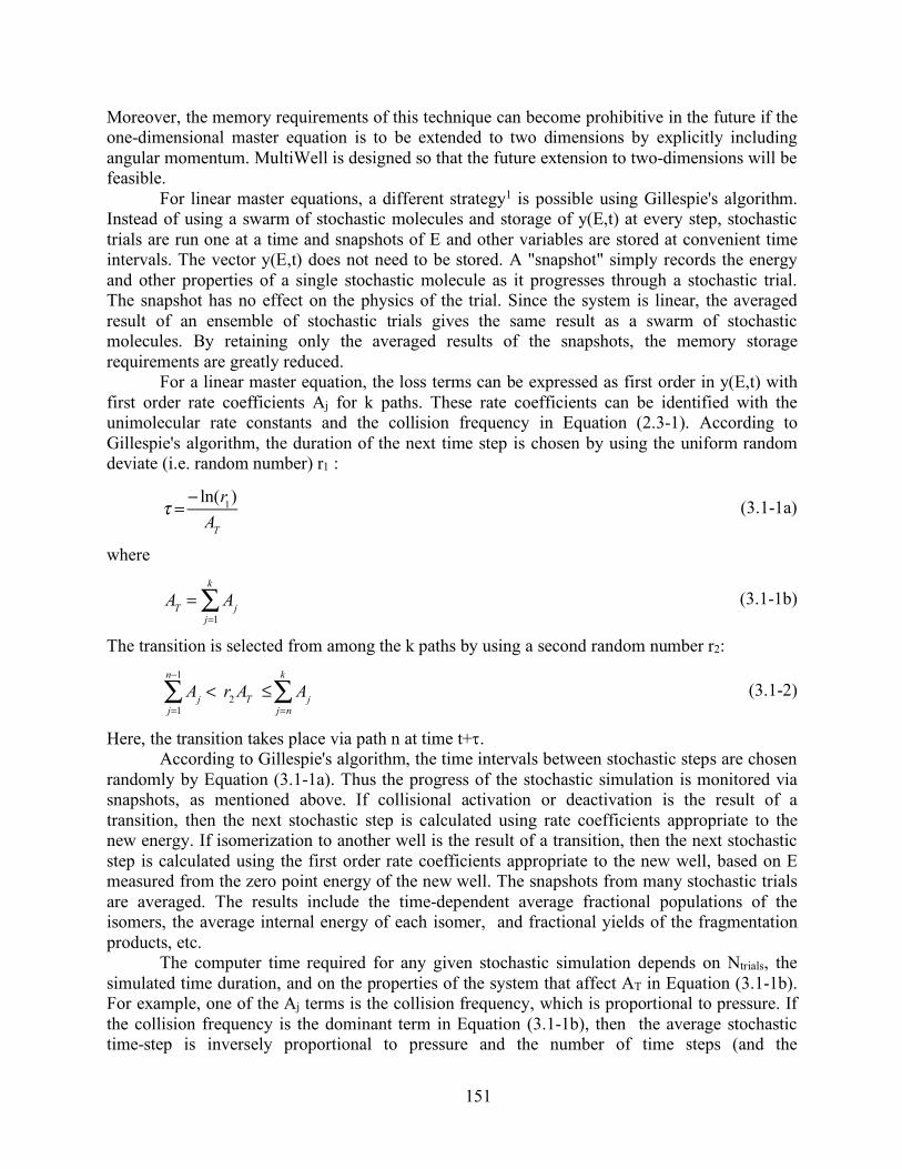
151

Moreover, the memory requirements of this technique can become prohibitive in the future if the one-dimensional master equation is to be extended to two dimensions by explicitly including angular momentum. MultiWell is designed so that the future extension to two-dimensions will be feasible.

For linear master equations, a different strategy1 is possible using Gillespie's algorithm. Instead of using a swarm of stochastic molecules and storage of y(E,t) at every step, stochastic trials are run one at a time and snapshots of E and other variables are stored at convenient time intervals. The vector y(E,t) does not need to be stored. A "snapshot" simply records the energy and other properties of a single stochastic molecule as it progresses through a stochastic trial. The snapshot has no effect on the physics of the trial. Since the system is linear, the averaged result of an ensemble of stochastic trials gives the same result as a swarm of stochastic molecules. By retaining only the averaged results of the snapshots, the memory storage requirements are greatly reduced.

For a linear master equation, the loss terms can be expressed as first order in y(E,t) with first order rate coefficients Aj for k paths. These rate coefficients can be identified with the unimolecular rate constants and the collision frequency in Equation (2.3-1). According to Gillespie's algorithm, the duration of the next time step is chosen by using the uniform random deviate (i.e. random number) r1 :

(3.1-1a)

where

(3.1-1b)

The transition is selected from among the k paths by using a second random number r2:

(3.1-2)

Here, the transition takes place via path n at time t+t. According to Gillespie's algorithm, the time intervals between stochastic steps are chosen

randomly by Equation (3.1-1a). Thus the progress of the stochastic simulation is monitored via snapshots, as mentioned above. If collisional activation or deactivation is the result of a transition, then the next stochastic step is calculated using rate coefficients appropriate to the new energy. If isomerization to another well is the result of a transition, then the next stochastic step is calculated using the first order rate coefficients appropriate to the new well, based on E measured from the zero point energy of the new well. The snapshots from many stochastic trials are averaged. The results include the time-dependent average fractional populations of the isomers, the average internal energy of each isomer, and fractional yields of the fragmentation products, etc.

The computer time required for any given stochastic simulation depends on Ntrials, the simulated time duration, and on the properties of the system that affect AT in Equation (3.1-1b). For example, one of the Aj terms is the collision frequency, which is proportional to pressure. If the collision frequency is the dominant term in Equation (3.1-1b), then the average stochastic time-step is inversely proportional to pressure and the number of time steps (and the

τ =

− ln(r1)AT

AT = Aj

j=1

k

∑

Aj

j=1

n−1

∑ < r2 AT ≤ Ajj=n

k

∑

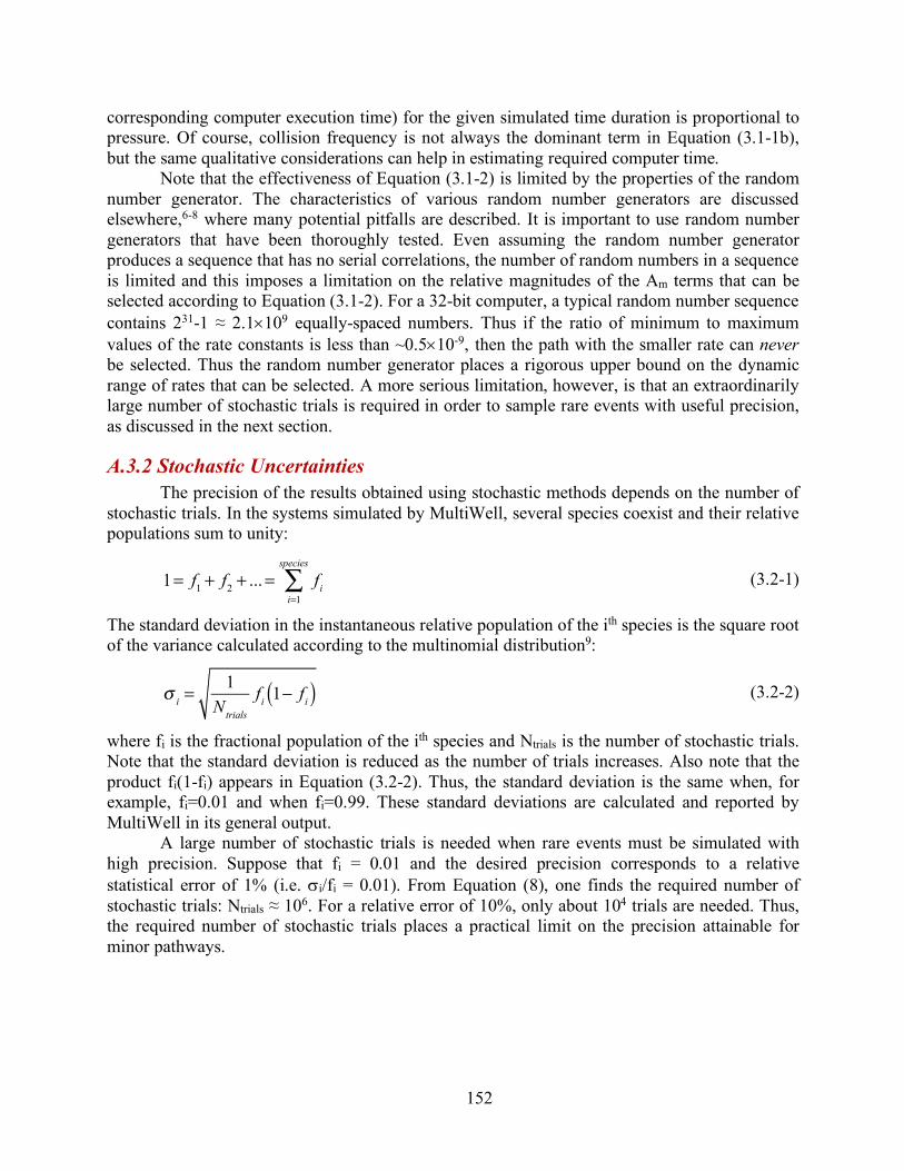
152

corresponding computer execution time) for the given simulated time duration is proportional to pressure. Of course, collision frequency is not always the dominant term in Equation (3.1-1b), but the same qualitative considerations can help in estimating required computer time.

Note that the effectiveness of Equation (3.1-2) is limited by the properties of the random number generator. The characteristics of various random number generators are discussed elsewhere,6-8 where many potential pitfalls are described. It is important to use random number generators that have been thoroughly tested. Even assuming the random number generator produces a sequence that has no serial correlations, the number of random numbers in a sequence is limited and this imposes a limitation on the relative magnitudes of the Am terms that can be selected according to Equation (3.1-2). For a 32-bit computer, a typical random number sequence contains 231-1 ≈ 2.1´109 equally-spaced numbers. Thus if the ratio of minimum to maximum values of the rate constants is less than ~0.5´10-9, then the path with the smaller rate can never be selected. Thus the random number generator places a rigorous upper bound on the dynamic range of rates that can be selected. A more serious limitation, however, is that an extraordinarily large number of stochastic trials is required in order to sample rare events with useful precision, as discussed in the next section.

A.3.2 Stochastic Uncertainties The precision of the results obtained using stochastic methods depends on the number of

stochastic trials. In the systems simulated by MultiWell, several species coexist and their relative populations sum to unity:

(3.2-1)

The standard deviation in the instantaneous relative population of the ith species is the square root of the variance calculated according to the multinomial distribution9:

(3.2-2)

where fi is the fractional population of the ith species and Ntrials is the number of stochastic trials. Note that the standard deviation is reduced as the number of trials increases. Also note that the product fi(1-fi) appears in Equation (3.2-2). Thus, the standard deviation is the same when, for example, fi=0.01 and when fi=0.99. These standard deviations are calculated and reported by MultiWell in its general output.

A large number of stochastic trials is needed when rare events must be simulated with high precision. Suppose that fi = 0.01 and the desired precision corresponds to a relative statistical error of 1% (i.e. si/fi = 0.01). From Equation (8), one finds the required number of stochastic trials: Ntrials ≈ 106. For a relative error of 10%, only about 104 trials are needed. Thus, the required number of stochastic trials places a practical limit on the precision attainable for minor pathways.

1= f1 + f2 + ...= fi

i=1

species

∑

σ i =

1Ntrials

fi 1− fi( )

153

References


(2) Gillespie, D. T. A general method for numerically simulating the stochastic time evolution of coupled chemical reactions. J. Comp. Phys. 1976, 22, 403-434.

(3) Gillespie, D. T. Exact stochastic simulation of coupled chemical reactions. J. Phys. Chem. 1977, 81, 2340-2361.

(4) Gillespie, D. T. Monte Carlo simulation of random walks with residence time dependent transition probability rates. J. Comp. Phys. 1978, 28, 395-407.

(5) Gillespie, D. T. A rigorous derivation of the chemical master equation. Physica A: Statistical and Theoretical Physics (Amsterdam) 1992, 188, 404-425.

(6) Knuth, D. E. Seminumerical Algorithms, 2 ed.; Addison-Wesley: Reading, MA, 1981; Vol. 2.

(7) Press, W. H.; Teukolsky, S. A. [Random number generators]. Computers in Physics 1992, 6, 522-524.


(9) Tsokos, C. P. Probability Distributions: An Introduction to Probability Theory with Applications; Wadsworth Publishing Company Inc.: Belmont CA, 1972.


(11) Vereecken, L.; Huyberechts, G.; Peeters, J. Stochastic simulation of chemically activated unimolecular reactions. J. Chem. Phys. 1997, 106, 6564-6573; https://doi.org/10.1063/1.473656.

A.4. Processes

A.4.1 Unimolecular Reactions The energy-dependent specific unimolecular rate constant k(E) is given by the RRKM

statistical theory12,15,16,20,30:

(4.1-1)

where m‡ and m are the number of optical isomers,16 sext‡ and sext are the external rotation symmetry numbers, and ge‡ and ge are the electronic state degeneracies of the transition state and reactant, respectively; h is Planck's constant, G‡(E-E0) is the sum of states of the transition state, E0 is the reaction threshold energy, and r(E) is the density of states of the reactant molecule. The

k(E) = m‡

mσ ext

σ ext‡

⎡

⎣⎢

⎤

⎦⎥

ge‡

ge

1h

G‡(E − E0 )ρ(E)

154

internal energy E is measured relative to the zero point energy of the reactant molecule and the reaction threshold energy (critical energy) is the difference between the zero point energies of reactant and transition state. Equation (4.1-1) was written by assuming that the rotational external symmetry numbers were not used in calculating the sums and densities of states.16 It is, however, assumed that internal rotor symmetry numbers are used explicitly in the sum and density calculations and hence do not appear in Equation (4.1-1). Note that the quantity set off in square brackets is the reaction path degeneracy.16

At low energies, where densities of states may be very sparse, r(E) may be very small or zero in a given energy grain (lower energy portion of the double array). In MultiWell, this is treated as if there are no reactant states in the energy grain: k(E) is set equal to zero in that grain. During evolution of the population distribution, population never resides in energy grains that do not contain reactant states.

Tight Transition States For a tight transition state, G‡(E-E0) can be calculated from a vibrational-rotational

assignment and the reaction threshold energy can be corrected approximately for angular momentum effects by using a pseudo-diatomic model.13,15,16 All polyatomics are treated by DenSum and MultiWell as SYMMETRIC TOPS with moments of inertia IA, IB = IC and corresponding rotational constants A = ħ2/2IA and B ==ħ2/2IB. The rotational energy of a symmetric top is given by

where quantum numbers J and K refer to the two-dimensional 2-D adiabatic rotor (i.e. the one that conserves angular momentum J) and to one-dimensional rotation about the top axis (projection of J on the top axis), respectively (see Appendix B.4). For a given value of J, quantum number K can take values from -J to +J, inclusive; all such states are doubly degenerate except for K=0, which is singly degenerate. In the present version of DenSum, the K-rotor is normally designated as a simple 1-D rotation (either quantized or classical). The moment of inertia for the K-rotor IK is given by

In many applications, IK ≈ IA. Because the K-rotor is normally designated as a simple rotation in MultiWell simulations,

the range of K is normally not restricted to ±J. When IA < IB (prolate top), then IK > 0. When IA > IB (oblate top), then IK < 0. If the K quantum number is not constrained to K ≤ |J|, then Er(J,K) can be <0. The unrestricted range of K is not serious a approximation for prolate tops, since the rotational energy is >0 for all values of J and K. For oblate tops, however, Er(J,K) can be <0 when K >> J. Thus the approximate treatment of the K-rotor may fail seriously for oblate tops. The kro degree of freedom type (see DenSum) employs the correct treatment for a user-specified value of J.

Thus the three external rotations of a non-linear molecule consist of a 1-dimensional rotor (the 1-D "K-rotor") and a 2-dimensional top (the 2-D adiabatic rotor). The K-ROTOR properties are listed in densum.dat and included in density and sums of states calculations. Pragmatically, IB is usually not equal to IC, since most chemical species are not true symmetric tops. For almost symmetric tops (where IB ≈ IC), one can use either of two reasonable approximations for I2D (see Appendix B.4):

Er J,K( ) = J J +1( )B + (A − B)K 2

IK = IA−1 − IB

−1⎡⎣ ⎤⎦−1

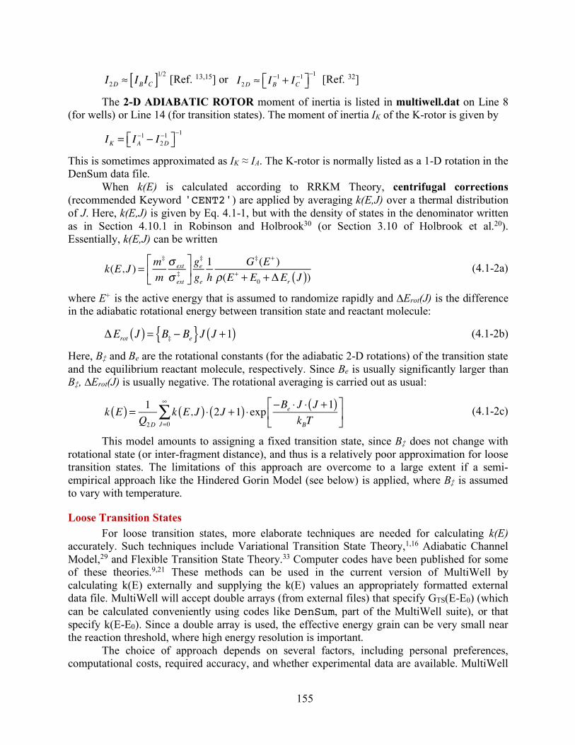
155

[Ref. 13,15] or [Ref. 32]

The 2-D ADIABATIC ROTOR moment of inertia is listed in multiwell.dat on Line 8 (for wells) or Line 14 (for transition states). The moment of inertia IK of the K-rotor is given by

This is sometimes approximated as IK ≈ IA. The K-rotor is normally listed as a 1-D rotation in the DenSum data file.

When k(E) is calculated according to RRKM Theory, centrifugal corrections (recommended Keyword 'CENT2') are applied by averaging k(E,J) over a thermal distribution of J. Here, k(E,J) is given by Eq. 4.1-1, but with the density of states in the denominator written as in Section 4.10.1 in Robinson and Holbrook30 (or Section 3.10 of Holbrook et al.20). Essentially, k(E,J) can be written

(4.1-2a)

where E+ is the active energy that is assumed to randomize rapidly and ∆Erot(J) is the difference in the adiabatic rotational energy between transition state and reactant molecule:

(4.1-2b)

Here, B‡ and Be are the rotational constants (for the adiabatic 2-D rotations) of the transition state and the equilibrium reactant molecule, respectively. Since Be is usually significantly larger than B‡, ∆Erot(J) is usually negative. The rotational averaging is carried out as usual:

(4.1-2c)

This model amounts to assigning a fixed transition state, since B‡ does not change with rotational state (or inter-fragment distance), and thus is a relatively poor approximation for loose transition states. The limitations of this approach are overcome to a large extent if a semi-empirical approach like the Hindered Gorin Model (see below) is applied, where B‡ is assumed to vary with temperature.

Loose Transition States For loose transition states, more elaborate techniques are needed for calculating k(E)

accurately. Such techniques include Variational Transition State Theory,1,16 Adiabatic Channel Model,29 and Flexible Transition State Theory.33 Computer codes have been published for some of these theories.9,21 These methods can be used in the current version of MultiWell by calculating k(E) externally and supplying the k(E) values an appropriately formatted external data file. MultiWell will accept double arrays (from external files) that specify GTS(E-E0) (which can be calculated conveniently using codes like DenSum, part of the MultiWell suite), or that specify k(E-E0). Since a double array is used, the effective energy grain can be very small near the reaction threshold, where high energy resolution is important.

The choice of approach depends on several factors, including personal preferences, computational costs, required accuracy, and whether experimental data are available. MultiWell

I2D ≈ IBIC[ ]1/2 I2D ≈ IB−1 + IC

−1⎡⎣ ⎤⎦−1

IK = IA−1 − I2D

−1⎡⎣ ⎤⎦−1

k(E, J ) = m‡

mσ ext

σ ext‡

⎡

⎣⎢

⎤

⎦⎥ge‡

ge

1h

G‡(E+ )ρ(E+ + E0 +∆ Er J( ))

∆ Erot J( ) = B‡ − Be{ }J J +1( )

k E( ) = 1Q2D

k E, J( ) ⋅ 2J +1( ) ⋅exp −Be ⋅ J ⋅ J +1( )kBT

⎡

⎣⎢

⎤

⎦⎥

J=0

∞

∑

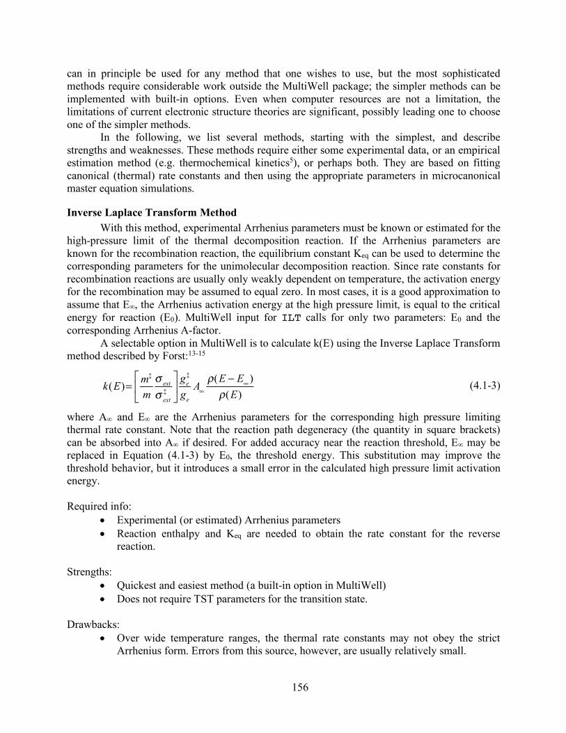
156

can in principle be used for any method that one wishes to use, but the most sophisticated methods require considerable work outside the MultiWell package; the simpler methods can be implemented with built-in options. Even when computer resources are not a limitation, the limitations of current electronic structure theories are significant, possibly leading one to choose one of the simpler methods.

In the following, we list several methods, starting with the simplest, and describe strengths and weaknesses. These methods require either some experimental data, or an empirical estimation method (e.g. thermochemical kinetics5), or perhaps both. They are based on fitting canonical (thermal) rate constants and then using the appropriate parameters in microcanonical master equation simulations.

Inverse Laplace Transform Method With this method, experimental Arrhenius parameters must be known or estimated for the

high-pressure limit of the thermal decomposition reaction. If the Arrhenius parameters are known for the recombination reaction, the equilibrium constant Keq can be used to determine the corresponding parameters for the unimolecular decomposition reaction. Since rate constants for recombination reactions are usually only weakly dependent on temperature, the activation energy for the recombination may be assumed to equal zero. In most cases, it is a good approximation to assume that E∞, the Arrhenius activation energy at the high pressure limit, is equal to the critical energy for reaction (E0). MultiWell input for ILT calls for only two parameters: E0 and the corresponding Arrhenius A-factor.

A selectable option in MultiWell is to calculate k(E) using the Inverse Laplace Transform method described by Forst:13-15

(4.1-3)

where A∞ and E∞ are the Arrhenius parameters for the corresponding high pressure limiting thermal rate constant. Note that the reaction path degeneracy (the quantity in square brackets) can be absorbed into A∞ if desired. For added accuracy near the reaction threshold, E∞ may be replaced in Equation (4.1-3) by E0, the threshold energy. This substitution may improve the threshold behavior, but it introduces a small error in the calculated high pressure limit activation energy.

Required info:

• Experimental (or estimated) Arrhenius parameters • Reaction enthalpy and Keq are needed to obtain the rate constant for the reverse

reaction. Strengths:

• Quickest and easiest method (a built-in option in MultiWell) • Does not require TST parameters for the transition state.

Drawbacks:

• Over wide temperature ranges, the thermal rate constants may not obey the strict Arrhenius form. Errors from this source, however, are usually relatively small.

k(E)= m‡

mσ ext

σ ext‡

⎡

⎣⎢

⎤

⎦⎥

ge‡

ge

A∞

ρ(E − E∞ )ρ(E)

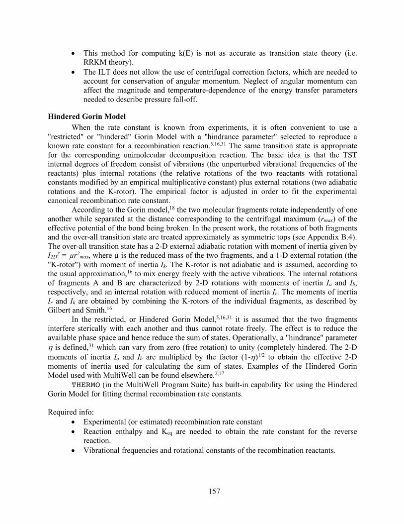
157

• This method for computing k(E) is not as accurate as transition state theory (i.e. RRKM theory).

• The ILT does not allow the use of centrifugal correction factors, which are needed to account for conservation of angular momentum. Neglect of angular momentum can affect the magnitude and temperature-dependence of the energy transfer parameters needed to describe pressure fall-off.

Hindered Gorin Model When the rate constant is known from experiments, it is often convenient to use a

"restricted" or "hindered" Gorin Model with a "hindrance parameter" selected to reproduce a known rate constant for a recombination reaction.5,16,31 The same transition state is appropriate for the corresponding unimolecular decomposition reaction. The basic idea is that the TST internal degrees of freedom consist of vibrations (the unperturbed vibrational frequencies of the reactants) plus internal rotations (the relative rotations of the two reactants with rotational constants modified by an empirical multiplicative constant) plus external rotations (two adiabatic rotations and the K-rotor). The empirical factor is adjusted in order to fit the experimental canonical recombination rate constant.

According to the Gorin model,18 the two molecular fragments rotate independently of one another while separated at the distance corresponding to the centrifugal maximum (rmax) of the effective potential of the bond being broken. In the present work, the rotations of both fragments and the over-all transition state are treated approximately as symmetric tops (see Appendix B.4). The over-all transition state has a 2-D external adiabatic rotation with moment of inertia given by I2D‡ = µr2max, where µ is the reduced mass of the two fragments, and a 1-D external rotation (the "K-rotor") with moment of inertia Ik. The K-rotor is not adiabatic and is assumed, according to the usual approximation,16 to mix energy freely with the active vibrations. The internal rotations of fragments A and B are characterized by 2-D rotations with moments of inertia Ia and Ib, respectively, and an internal rotation with reduced moment of inertia Ir. The moments of inertia Ir and Ik are obtained by combining the K-rotors of the individual fragments, as described by Gilbert and Smith.16

In the restricted, or Hindered Gorin Model,5,16,31 it is assumed that the two fragments interfere sterically with each another and thus cannot rotate freely. The effect is to reduce the available phase space and hence reduce the sum of states. Operationally, a "hindrance" parameter h is defined,31 which can vary from zero (free rotation) to unity (completely hindered. The 2-D moments of inertia Ia and Ib are multiplied by the factor (1-h)1/2 to obtain the effective 2-D moments of inertia used for calculating the sum of states. Examples of the Hindered Gorin Model used with MultiWell can be found elsewhere.2,17

THERMO (in the MultiWell Program Suite) has built-in capability for using the Hindered Gorin Model for fitting thermal recombination rate constants.

Required info:

• Experimental (or estimated) recombination rate constant • Reaction enthalpy and Keq are needed to obtain the rate constant for the reverse

reaction. • Vibrational frequencies and rotational constants of the recombination reactants.

158

• An assumed function for V(r) along the reaction coordinate (usually a Morse or Varshni potential) described by the center-of-mass distance between the two reactants.

Strengths:

• Relatively easy method. • Generates TST parameters that fit the experimental canonical recombination rate

constant at a given temperature. • TST (i.e. RRKM) is a proven method; centrifugal corrections are employed.

Drawbacks: • Experimental or estimated rate constants are required at every temperature. • Fitting of the rate constants must be carried out at each temperature. • TST parameters are different at each temperature. • Separable harmonic oscillator and rigid rotor approximations may not be sufficiently

accurate. Using separable hindered internal rotations is significantly more accurate, but more expensive.

Semi-empirical Canonical Variational Transition State Theory We are currently using Semi-empirical Canonical Variational Transition State Theory

(VTST) for applications where electronic structure methods are not reliable, but can still supply useful information. The basic idea is to use methods like Density Functional Theory (DFT; e.g. B3LYP) and large basis sets to carry out constrained optimizations at fixed distances along a reaction path in order to obtain the rotational constants and the vibrational frequencies orthogonal to the path, but then use empirical expressions for V(r), the potential energy along the path. For example, we have used V(r) = −Cr−n, where C is a constant and n = 6.

The vibrational frequencies, rotational constants, and V(r) vary with position along the path. At each of the fixed points along the path, one can use those quantities as input to THERMO (in the MultiWell Program Suite) for computing a trial rate constant for the thermal reaction. The minimum trial rate constant corresponds to the VTST rate constant. The minimum rate constant is best obtained by interpolation between the fixed points, but for points separated by 0.1 Å or less it is almost as good to use the lowest trial rate constant, without interpolation. We find that by varying the constant C, it is possible to fit the experimental recombination rate constant at a given temperature (e.g. 298 K). According to our limited experience with this method, the value of the constant C fitted at a single temperature is in reasonable agreement with the temperature dependence of the recombination reaction, when known.

For a master equation simulation at temperature T, one uses the transition state parameters (vibrational frequencies, rotational constants, and V(r)) corresponding to the variational transition state at T.

Required info:

• Experimental (or estimated) recombination rate constant • Reaction enthalpy and Keq are needed to obtain the rate constant for the reverse

reaction. • Constrained geometry optimizations at fixed distances along the reaction path; and

corresponding vibrational frequencies and rotational constants.

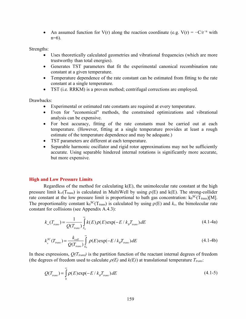
159

• An assumed function for V(r) along the reaction coordinate (e.g. V(r) = −C/r−n with n=6).

Strengths:

• Uses theoretically calculated geometries and vibrational frequencies (which are more trustworthy than total energies).

• Generates TST parameters that fit the experimental canonical recombination rate constant at a given temperature.

• Temperature dependence of the rate constant can be estimated from fitting to the rate constant at a single temperature.

• TST (i.e. RRKM) is a proven method; centrifugal corrections are employed.

Drawbacks: • Experimental or estimated rate constants are required at every temperature. • Even for "economical" methods, the constrained optimizations and vibrational

analysis can be expensive. • For best accuracy, fitting of the rate constants must be carried out at each

temperature. (However, fitting at a single temperature provides at least a rough estimate of the temperature dependence and may be adequate.)

• TST parameters are different at each temperature. • Separable harmonic oscillator and rigid rotor approximations may not be sufficiently

accurate. Using separable hindered internal rotations is significantly more accurate, but more expensive.

High and Low Pressure Limits Regardless of the method for calculating k(E), the unimolecular rate constant at the high

pressure limit k∞(Ttrans) is calculated in MultiWell by using r(E) and k(E). The strong-collider rate constant at the low pressure limit is proportional to bath gas concentration: k0SC(Ttrans)[M]. The proportionality constant k0SC(Ttrans) is calculated by using r(E) and kc, the bimolecular rate constant for collisions (see Appendix A.4.3):

(4.1-4a)

(4.1-4b)

In these expressions, Q(Ttrans) is the partition function of the reactant internal degrees of freedom (the degrees of freedom used to calculate r(E) and k(E)) at translational temperature Ttrans:

(4.1-5)

k∞(Ttrans ) =

1Q(Ttrans )

k(E)ρ(E)exp(−E / kBTtrans )dEE0

∞

∫

k0

SC (Ttrans ) =kcoll

Q(Ttrans )ρ(E)exp(−E / kBTtrans )dE

E0

∞

∫

Q(Ttrans ) = ρ(E)exp(−E / kBTtrans )dE

0

∞

∫

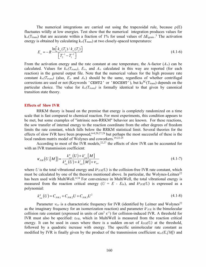
160

The numerical integrations are carried out using the trapezoidal rule, because r(E) fluctuates wildly at low energies. Test show that the numerical integration produces values for k∞(Ttrans) that are accurate within a fraction of 1% for usual values of ∆Egrain .3 The activation energy is obtained by calculating k∞(Ttrans) at two closely-spaced temperatures:

(4.1-6)

From the activation energy and the rate constant at one temperature, the A-factor (A∞) can be calculated. Values for k∞(Ttrans), E∞, and A∞ calculated in this way are reported (for each reaction) in the general output file. Note that the numerical values for the high pressure rate constant k∞(Ttrans) (also, E∞ and A∞) should be the same, regardless of whether centrifugal corrections are used or not (Keywords 'CENT2' or 'NOCENT'), but k0SC(Ttrans) depends on the particular choice. The value for k∞(Ttrans) is formally identical to that given by canonical transition state theory.

Effects of Slow IVR RRKM theory is based on the premise that energy is completely randomized on a time

scale that is fast compared to chemical reaction. For most experiments, this condition appears to be met, but some examples of "intrinsic non-RRKM" behavior are known. For these reactions, the sow transfer of internal energy to the reaction coordinate from the other degrees of freedom limits the rate constant, which falls below the RRKM statistical limit. Several theories for the effects of slow IVR have been proposed,6-8,20,27,28 but perhaps the most successful of these is the local random matrix model of Wolynes and coworkers.19,22-25

According to most of the IVR models,22,27 the effects of slow IVR can be accounted for with an IVR transmission coefficient:

(4.1-7)

where U is the total vibrational energy and kqIVR(U) is the collision-free IVR rate constant, which must be calculated by one of the theories mentioned above. In particular, the Wolynes-Leitner22 has been used with MultiWell.4,34 For convenience in MultiWell, the total vibrational energy is measured from the reaction critical energy (U = E - E0r), and kqIVR(U) is expressed as a polynomial:

(4.1-8)

Parameter nivr is a characteristic frequency for IVR (identified by Leitner and Wolynes22 as the imaginary frequency for an isomerization reaction) and parameter kcIVR is the bimolecular collision rate constant (expressed in units of cm3 s-1) for collision-induced IVR. A threshold for IVR must also be specified: tIVR, which in MultiWell is measured from the reaction critical energy. It can be used in cases where there is a sudden on-set of kIVR(U) at the threshold, followed by a quadratic increase with energy. The specific unimolecular rate constant as modified by IVR is finally given by the product of the transmission coefficient kivr(E,[M]) and

E∞ = −R

ln k∞(T2 ) / k∞(T1)⎡⎣ ⎤⎦T2

−1 −T1−1⎡⎣ ⎤⎦

κ IVR U, M[ ]( ) = kIVR

q U( ) + kIVR

c M[ ]k

IVR

q U( ) + kIVR

c M[ ]+ν ivr

kIVR

q U( ) = CIVR,1 +CIVR,2U +CIVR,3U2

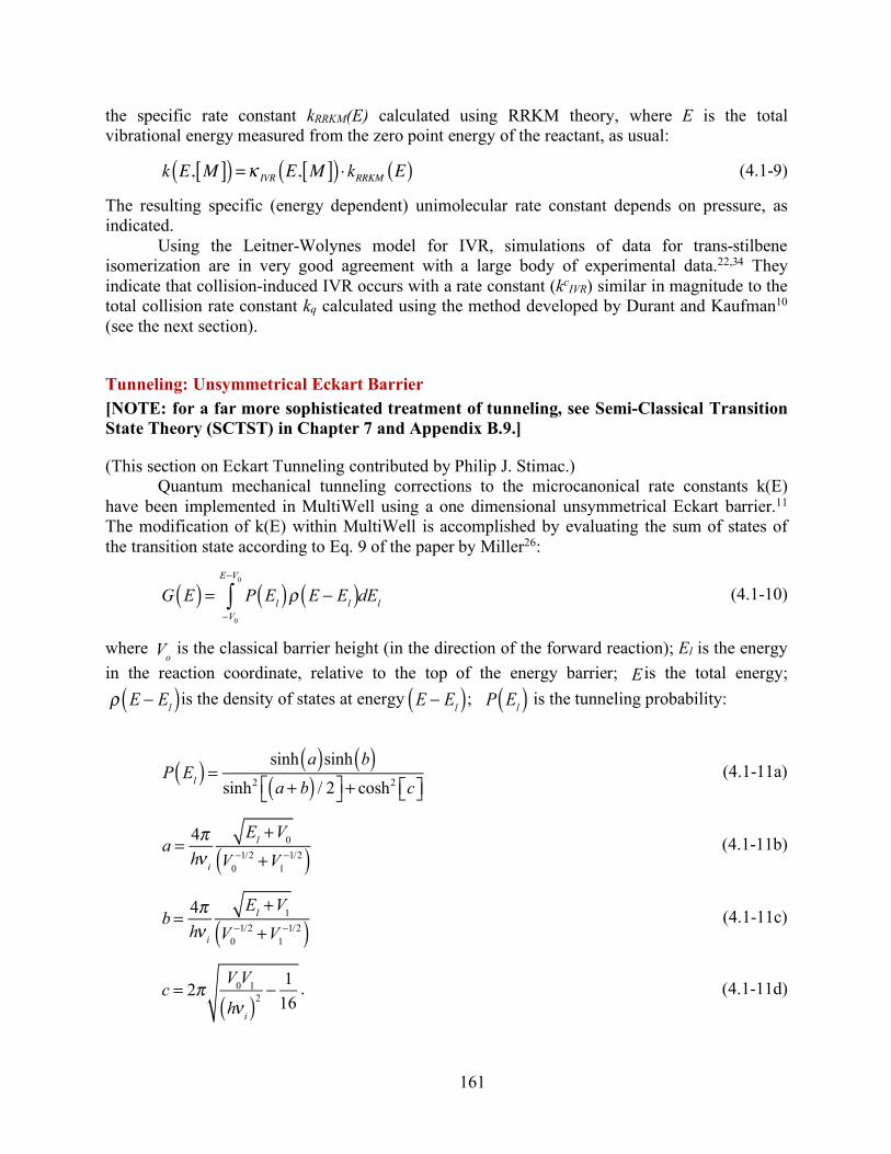
161

the specific rate constant kRRKM(E) calculated using RRKM theory, where E is the total vibrational energy measured from the zero point energy of the reactant, as usual:

(4.1-9)

The resulting specific (energy dependent) unimolecular rate constant depends on pressure, as indicated.

Using the Leitner-Wolynes model for IVR, simulations of data for trans-stilbene isomerization are in very good agreement with a large body of experimental data.22,34 They indicate that collision-induced IVR occurs with a rate constant (kcIVR) similar in magnitude to the total collision rate constant kq calculated using the method developed by Durant and Kaufman10 (see the next section).

Tunneling: Unsymmetrical Eckart Barrier [NOTE: for a far more sophisticated treatment of tunneling, see Semi-Classical Transition State Theory (SCTST) in Chapter 7 and Appendix B.9.]

(This section on Eckart Tunneling contributed by Philip J. Stimac.) Quantum mechanical tunneling corrections to the microcanonical rate constants k(E)

have been implemented in MultiWell using a one dimensional unsymmetrical Eckart barrier.11 The modification of k(E) within MultiWell is accomplished by evaluating the sum of states of the transition state according to Eq. 9 of the paper by Miller26:

(4.1-10)

where is the classical barrier height (in the direction of the forward reaction); El is the energy in the reaction coordinate, relative to the top of the energy barrier; is the total energy;

is the density of states at energy ; is the tunneling probability:

(4.1-11a)

(4.1-11b)

(4.1-11c)

. (4.1-11d)

k E, M[ ]( ) =κ IVR E, M[ ]( ) ⋅ kRRKM E( )

G E( ) = P El( )ρ E − El( )

−V0

E−V0

∫ dEl

Vo

E

ρ E − El( ) E − El( ) P El( )

P El( ) = sinh a( )sinh b( )

sinh2 a + b( ) / 2⎡⎣ ⎤⎦ + cosh2 c⎡⎣ ⎤⎦

a = 4π

hν i

El +V0

V0−1/2 +V1

−1/2( )

b = 4π

hν i

El +V1

V0−1/2 +V1

−1/2( )

c = 2πV0V1

hν i( )2 −1

16

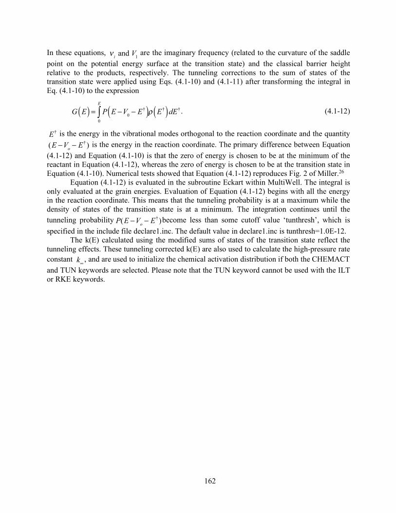
162

In these equations, are the imaginary frequency (related to the curvature of the saddle point on the potential energy surface at the transition state) and the classical barrier height relative to the products, respectively. The tunneling corrections to the sum of states of the transition state were applied using Eqs. (4.1-10) and (4.1-11) after transforming the integral in Eq. (4.1-10) to the expression

. (4.1-12)

is the energy in the vibrational modes orthogonal to the reaction coordinate and the quantity is the energy in the reaction coordinate. The primary difference between Equation

(4.1-12) and Equation (4.1-10) is that the zero of energy is chosen to be at the minimum of the reactant in Equation (4.1-12), whereas the zero of energy is chosen to be at the transition state in Equation (4.1-10). Numerical tests showed that Equation (4.1-12) reproduces Fig. 2 of Miller.26

Equation (4.1-12) is evaluated in the subroutine Eckart within MultiWell. The integral is only evaluated at the grain energies. Evaluation of Equation (4.1-12) begins with all the energy in the reaction coordinate. This means that the tunneling probability is at a maximum while the density of states of the transition state is at a minimum. The integration continues until the tunneling probability become less than some cutoff value ‘tunthresh’, which is specified in the include file declare1.inc. The default value in declare1.inc is tunthresh=1.0E-12.

The k(E) calculated using the modified sums of states of the transition state reflect the tunneling effects. These tunneling corrected k(E) are also used to calculate the high-pressure rate constant , and are used to initialize the chemical activation distribution if both the CHEMACT and TUN keywords are selected. Please note that the TUN keyword cannot be used with the ILT or RKE keywords.

ν i and V1

G E( ) = P E −V0 − E†( )

0

E

∫ ρ E†( )dE†

E†

(E −Vo − E† )

P(E −Vo − E† )

k∞

163

References


(2) Barker, J. R.; Lohr, L. L.; Shroll, R. M.; Reading, S. Modeling the Organic Nitrate Yields in the Reaction of Alkyl Peroxy Radicals with Nitric Oxide. II. Reaction Simulations. J. Phys. Chem. A. 2003, 107, 7434-7444.


(4) Barker, J. R.; Ortiz, N. F.; Preses, J. M.; Lohr, L. L.; Maranzana, A.; Stimac, P. J. MultiWell-1.5.1 Software (Development version) Ann Arbor, Michigan, USA, 2005.

(5) Benson, S. W. Thermochemical Kinetics, 2nd ed.; Wiley: New York, 1976. (6) Bolton, K.; Nordholm, S. Beats in internal vibrational energy redistribution in trans-

stilbene - A study of the quantum and classical correspondence. Chemical Physics 1996, 207, 63-76.

(7) Bolton, K.; Nordholm, S. A classical molecular dynamics study of the intramolecular energy transfer of model trans-stilbene. Chemical Physics 1996, 203, 101-126.

(8) Bolton, K.; Nordholm, S. Classical trajectory study of collision induced intramolecular energy transfer in trans-stilbene. Chemical Physics 1996, 206, 103-128.

(9) Chuang, Y.-Y.; Corchado, J. C.; Fast, P. L.; Villà, J.; Hu, W.-P.; Liu, Y.-P.; Lynch, G. C.; Nguyen, K. A.; Jackels, C. F.; Gu, M. Z.; Rossi, I.; Coitiño, E. L.; Clayton, S.; Melissas, V. S.; Steckler, R.; Garrett, B. C.; Isaacson, A. D.; Truhlar, D. G. POLYRATE-version 8.1; University of Minnesota,: Minneapolis, MN, 1999.


(11) Eckart, C. The Penetration of a Potential Barrier by Electrons. Phys. Rev. 1930, 35, 1303-1309.

(12) Forst, W. Unimolecular rate theory test in thermal reactions. J. Phys. Chem. 1972, 76, 342-348; https://doi.org/10.1021/j100647a012.

(13) Forst, W. Theory of Unimolecular Reactions; Academic Press: New York, 1973. (14) Forst, W. Temperature-dependent A factor in thermal unimolecular reactions. J. Phys.

Chem. 1983, 83, 100-108. (15) Forst, W. Unimolecular Reactions. A Concise Introduction; Cambridge University Press:

Cambridge, 2003. (16) Gilbert, R. G.; Smith, S. C. Theory of Unimolecular and Recombination Reactions;

Blackwell Scientific Publications: Oxford, 1990. (17) Golden, D. M.; Barker, J. R.; Lohr, L. L. Master Equation Models for the Pressure- and

Temperature-Dependent Reactions HO + NO2 -> HONO2 and HO + NO2 -> HOONO. JPCA 2003, 107, 11057-11071.

(18) Gorin, E. Photolysis of acetaldehyde in the presence of iodine. Acta Physicochim., URSS 1938, 9, 681.

(19) Gruebele, M.; Wolynes, P. G. Vibrational energy flow and chemical reactions. Accounts of Chemical Research 2004, 37, 261-267.

164


(21) Klippenstein, S. J.; Wagner, A. F.; Robertson, S. H.; Dunbar, R.; Wardlaw, D. M. VariFlex Software; 1.0 ed.; Argonne National Laboratory, 1999.

(22) Leitner, D. M.; Levine, B.; Quenneville, J.; Martinez, T. J.; Wolynes, P. G. Quantum energy flow and trans-stilbene photoisomerization: an example of a non-RRKM reaction. Journal of Physical Chemistry A 2003, 107, 10706-10716.

(23) Leitner, D. M.; Wolynes, P. G. Many-dimensional quantum energy flow at low energy. Phys. Rev. Lett. 1996, 76, 216-219.

(24) Leitner, D. M.; Wolynes, P. G. Models of intramolecular energy redistribution spanning deterministic and statistical approaches: Comparison with experiment - Comment. ACH Models Chem. 1997, 134, 658-659.

(25) Leitner, D. M.; Wolynes, P. G. Quantum energy flow during molecular isomerization. Chemical Physics Letters 1997, 280, 411-418.

(26) Miller, W. H. Tunneling Corrections to Unimolecular Rate Constants, with Application to Formaldehyde. JACS 1979, 101, 6810-6814.

(27) Nordholm, S.; Back, A. On the role of nonergodicity and slow IVR in unimolecular reaction rate theory - A review and a view. Physical Chemistry Chemical Physics 2001, 3, 2289-2295.

(28) Oref, I.; Rabinovitch, B. S. Do Highly Excited Polyatomic Molecules Behave Ergodically? Accounts of Chemical Research 1979, 12, 166-175.

(29) Quack, M.; Troe, J. Specific rate constants of unimolecular processes. II. Adiabatic channel model. Ber. Bunsen-Ges. Phys. Chem. 1974, 78, 240-252.


(31) Smith, G. P.; Golden, D. M. Application of RRKM Theory to Reactions OH+NO2+N2 = HONO2+N2 (1) and ClO+NO2+N2 = ClONO2+N2 (2) - Modified Gorin Model Transition-State. IJCK 1978, 10, 489.

(32) Townes, C. H.; Schlalow, A. L. Microwave Spectroscopy; McGraw-Hill: New York, 1955.

(33) Wardlaw, D. W.; Marcus, R. A. RRKM reaction rate theory for transition states of any looseness. J. Chem. Phys. 1984, 110, 230-234.

(34) Weston, R. E., Jr.; Barker, J. R. On modeling the pressure-dependent photoisomerization of trans-stilbene by including slow intramolecular vibrational redistribution. J. Phys. Chem. A. 2006, 110, 7888-7897; DOI: 10.1021/jp061630b.

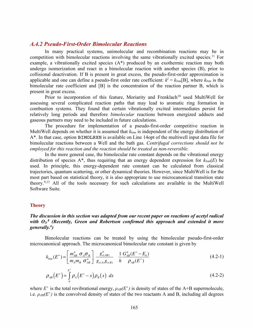
165

A.4.2 Pseudo-First-Order Bimolecular Reactions In many practical systems, unimolecular and recombination reactions may be in

competition with bimolecular reactions involving the same vibrationally excited species.11 For example, a vibrationally excited species (A*) produced by an exothermic reaction may both undergo isomerization and react in a bimolecular reaction with another species (B), prior to collisional deactivation. If B is present in great excess, the pseudo-first-order approximation is applicable and one can define a pseudo-first order rate coefficient: kI = kbim[B], where kbim is the bimolecular rate coefficient and [B] is the concentration of the reaction partner B, which is present in great excess.

Prior to incorporation of this feature, Moriarity and Frenklach10 used MultiWell for assessing several complicated reaction paths that may lead to aromatic ring formation in combustion systems. They found that certain vibrationally excited intermediates persist for relatively long periods and therefore bimolecular reactions between energized adducts and gaseous partners may need to be included in future calculations.

The procedure for implementation of a pseudo-first-order competitive reaction in MultiWell depends on whether it is assumed that kbim is independent of the energy distribution of A*. In that case, option BIMOLRXN is available on Line 14opt of the multiwell input data file for bimolecular reactions between a Well and the bath gas. Centrifugal corrections should not be employed for this reaction and the reaction should be treated as non-reversible.

In the more general case, the bimolecular rate constant depends on the vibrational energy distribution of species A*, thus requiring that an energy dependent expression for kbim(E) be used. In principle, this energy-dependent rate constant can be calculated from classical trajectories, quantum scattering, or other dynamical theories. However, since MultiWell is for the most part based on statistical theory, it is also appropriate to use microcanonical transition state theory.9,13 All of the tools necessary for such calculations are available in the MultiWell Software Suite.

Theory

The discussion in this section was adapted from our recent paper on reactions of acetyl radical with O2.8 (Recently, Green and Robertson confirmed this approach and extended it more generally.6)

Bimolecular reactions can be treated by using the bimolecular pseudo-first-order microcanonical approach. The microcanonical bimolecular rate constant is given by

(4.2-1)

(4.2-2)

where E+ is the total rovibrational energy, ρAB(E+) is density of states of the A+B supermolecule, i.e. ρAB(E+) is the convolved density of states of the two reactants A and B, including all degrees

kbim (E+ ) = mAB≠ σ Aσ B

mAmB σ AB≠

⎡

⎣⎢

⎤

⎦⎥

ge(AB)≠

ge(A)ge(B)

1hGAB

≠ (E+ − E0 )ρAB(E+ )

ρAB E+( ) = ρA E+ − x( )ρB x( ) dx0

E+

∫

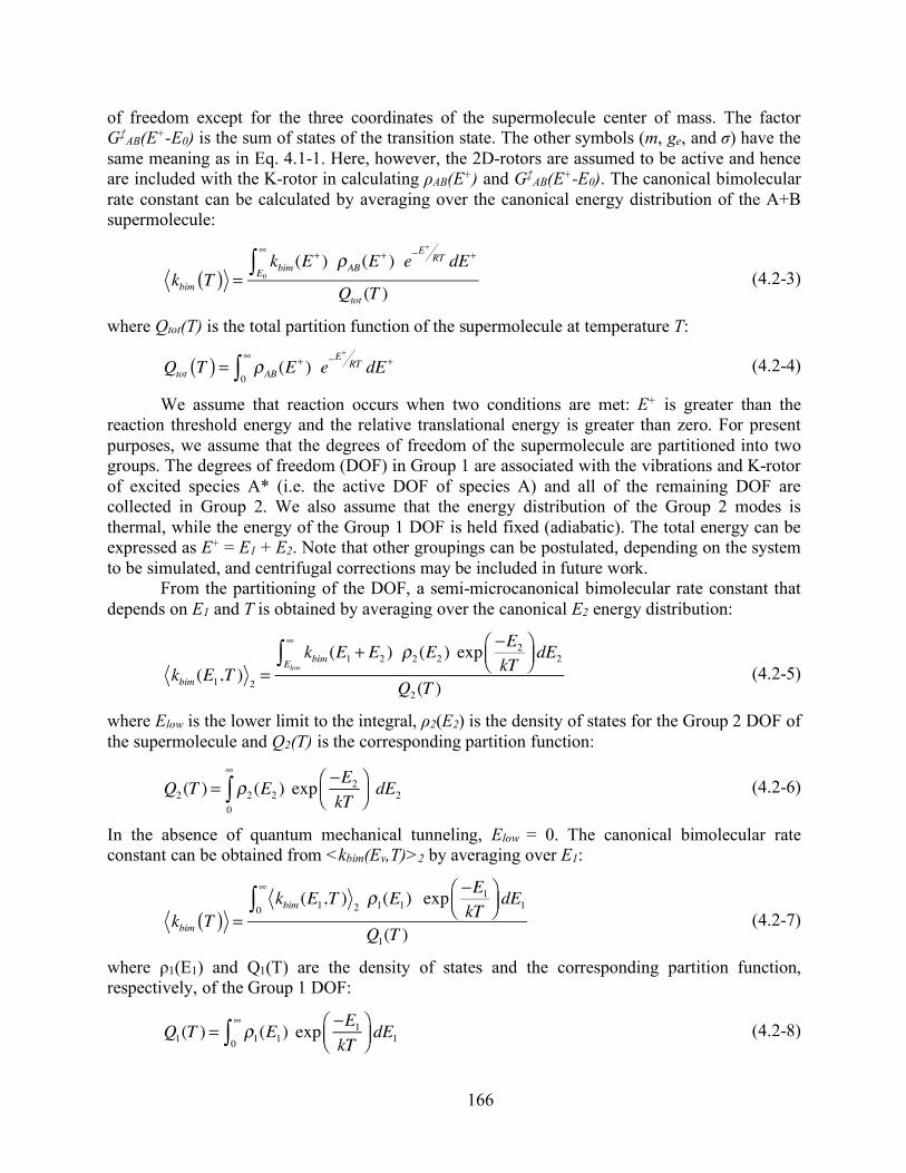
166

of freedom except for the three coordinates of the supermolecule center of mass. The factor G‡AB(E+-E0) is the sum of states of the transition state. The other symbols (m, ge, and σ) have the same meaning as in Eq. 4.1-1. Here, however, the 2D-rotors are assumed to be active and hence are included with the K-rotor in calculating ρAB(E+) and G‡AB(E+-E0). The canonical bimolecular rate constant can be calculated by averaging over the canonical energy distribution of the A+B supermolecule:

(4.2-3)

where Qtot(T) is the total partition function of the supermolecule at temperature T:

(4.2-4)

We assume that reaction occurs when two conditions are met: E+ is greater than the reaction threshold energy and the relative translational energy is greater than zero. For present purposes, we assume that the degrees of freedom of the supermolecule are partitioned into two groups. The degrees of freedom (DOF) in Group 1 are associated with the vibrations and K-rotor of excited species A* (i.e. the active DOF of species A) and all of the remaining DOF are collected in Group 2. We also assume that the energy distribution of the Group 2 modes is thermal, while the energy of the Group 1 DOF is held fixed (adiabatic). The total energy can be expressed as E+ = E1 + E2. Note that other groupings can be postulated, depending on the system to be simulated, and centrifugal corrections may be included in future work.

From the partitioning of the DOF, a semi-microcanonical bimolecular rate constant that depends on E1 and T is obtained by averaging over the canonical E2 energy distribution:

(4.2-5)

where Elow is the lower limit to the integral, ρ2(E2) is the density of states for the Group 2 DOF of the supermolecule and Q2(T) is the corresponding partition function:

(4.2-6)

In the absence of quantum mechanical tunneling, Elow = 0. The canonical bimolecular rate constant can be obtained from <kbim(Ev,T)>2 by averaging over E1:

(4.2-7)

where ρ1(E1) and Q1(T) are the density of states and the corresponding partition function, respectively, of the Group 1 DOF:

(4.2-8)

kbim T( ) =kbim (E+ ) ρAB(E+ ) e−

E+

RT dE+

E0

∞

∫Qtot (T )

Qtot T( ) = ρAB(E+ ) e−E+

RT dE+

0

∞

∫

kbim (E1,T )2=

kbim (E1 + E2 ) ρ2 (E2 )Elow

∞

∫ exp −E2

kT⎛⎝⎜

⎞⎠⎟ dE2

Q2 (T )

Q2 (T ) = ρ2 (E2 ) exp −E2

kT⎛⎝⎜

⎞⎠⎟

0

∞

∫ dE2

kbim T( ) =kbim (E1,T )

2 ρ1(E1) exp −E1

kT⎛⎝⎜

⎞⎠⎟ dE10

∞

∫Q1(T )

Q1(T ) = ρ1(E1) exp −E1

kT⎛⎝⎜

⎞⎠⎟ dE10

∞

∫

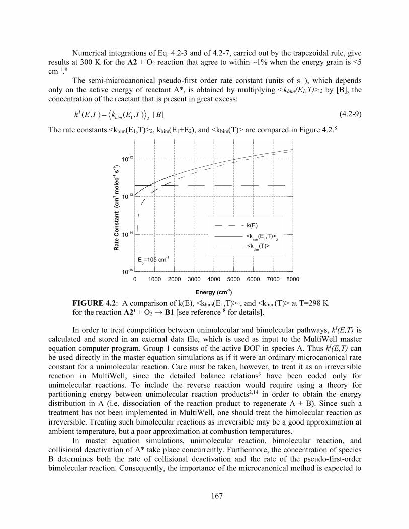
167

Numerical integrations of Eq. 4.2-3 and of 4.2-7, carried out by the trapezoidal rule, give results at 300 K for the A2 + O2 reaction that agree to within ~1% when the energy grain is ≤5 cm-1.8

The semi-microcanonical pseudo-first order rate constant (units of s-1), which depends only on the active energy of reactant A*, is obtained by multiplying <kbim(E1,T)>2 by [B], the concentration of the reactant that is present in great excess:

(4.2-9)

The rate constants <kbim(E1,T)>2, kbim(E1+E2), and <kbim(T)> are compared in Figure 4.2.8

FIGURE 4.2: A comparison of k(E), <kbim(E1,T)>2, and <kbim(T)> at T=298 K for the reaction A2' + O2 → B1 [see reference 8 for details].

In order to treat competition between unimolecular and bimolecular pathways, kI(E,T) is calculated and stored in an external data file, which is used as input to the MultiWell master equation computer program. Group 1 consists of the active DOF in species A. Thus kI(E,T) can be used directly in the master equation simulations as if it were an ordinary microcanonical rate constant for a unimolecular reaction. Care must be taken, however, to treat it as an irreversible reaction in MultiWell, since the detailed balance relations3 have been coded only for unimolecular reactions. To include the reverse reaction would require using a theory for partitioning energy between unimolecular reaction products2,14 in order to obtain the energy distribution in A (i.e. dissociation of the reaction product to regenerate A + B). Since such a treatment has not been implemented in MultiWell, one should treat the bimolecular reaction as irreversible. Treating such bimolecular reactions as irreversible may be a good approximation at ambient temperature, but a poor approximation at combustion temperatures.

In master equation simulations, unimolecular reaction, bimolecular reaction, and collisional deactivation of A* take place concurrently. Furthermore, the concentration of species B determines both the rate of collisional deactivation and the rate of the pseudo-first-order bimolecular reaction. Consequently, the importance of the microcanonical method is expected to

k I (E,T ) = kbim (E1,T ) 2 [B]

10-15

10-14

10-13

10-12

0 1000 2000 3000 4000 5000 6000 7000 8000

k(E)

<kbim

(E1,T)>

2

<kbim

(T)>

Rat

e C

onst

ant

(cm

3 mol

ec-1 s

-1)

Energy (cm-1)

E0=105 cm-1

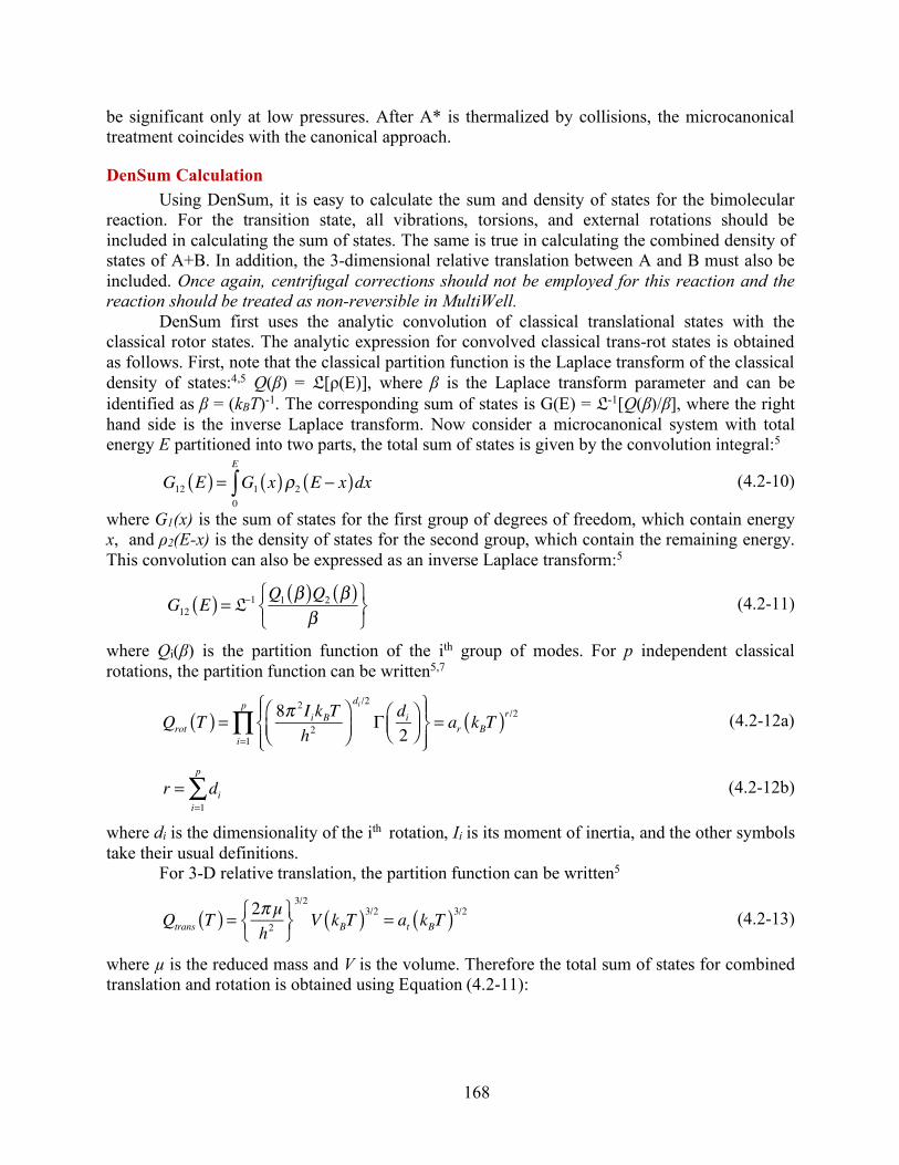
168

be significant only at low pressures. After A* is thermalized by collisions, the microcanonical treatment coincides with the canonical approach.

DenSum Calculation Using DenSum, it is easy to calculate the sum and density of states for the bimolecular

reaction. For the transition state, all vibrations, torsions, and external rotations should be included in calculating the sum of states. The same is true in calculating the combined density of states of A+B. In addition, the 3-dimensional relative translation between A and B must also be included. Once again, centrifugal corrections should not be employed for this reaction and the reaction should be treated as non-reversible in MultiWell.

DenSum first uses the analytic convolution of classical translational states with the classical rotor states. The analytic expression for convolved classical trans-rot states is obtained as follows. First, note that the classical partition function is the Laplace transform of the classical density of states:4,5 Q(β) = L[ρ(E)], where β is the Laplace transform parameter and can be identified as β = (kBT)-1. The corresponding sum of states is G(E) = L-1[Q(β)/β], where the right hand side is the inverse Laplace transform. Now consider a microcanonical system with total energy E partitioned into two parts, the total sum of states is given by the convolution integral:5

(4.2-10)

where G1(x) is the sum of states for the first group of degrees of freedom, which contain energy x, and ρ2(E-x) is the density of states for the second group, which contain the remaining energy. This convolution can also be expressed as an inverse Laplace transform:5

(4.2-11)

where Qi(β) is the partition function of the ith group of modes. For p independent classical rotations, the partition function can be written5,7

(4.2-12a)

(4.2-12b)

where di is the dimensionality of the ith rotation, Ii is its moment of inertia, and the other symbols take their usual definitions.

For 3-D relative translation, the partition function can be written5

(4.2-13)

where µ is the reduced mass and V is the volume. Therefore the total sum of states for combined translation and rotation is obtained using Equation (4.2-11):

G12 E( ) = G1 x( )ρ2 E − x( )dx0

E

∫

G12 E( ) = L−1 Q1 β( )Q2 β( )

β⎧⎨⎩

⎫⎬⎭

Qrot T( ) = 8π 2IikBTh2

⎛⎝⎜

⎞⎠⎟

di /2

Γ di2

⎛⎝⎜

⎞⎠⎟

⎧⎨⎪

⎩⎪

⎫⎬⎪

⎭⎪i=1

p

∏ = ar kBT( )r/2

r = dii=1

p

∑

Qtrans T( ) = 2π µh2

⎧⎨⎩

⎫⎬⎭

3/2

V kBT( )3/2 = at kBT( )3/2

169

(4.2-14)

When no rotations are present, the sum of states is just the sum of translational states:5,13

(4.2-15)

These expressions are used by DenSum to calculate the number of states in each energy bin when initializing the sums of states array, according to the Astholz et al.1 modification of the Stein-Rabinovitch state-counting method.12

Grt E( ) = aratL−1 p−1−(r+3)/2( ) = 2aratEr+3( )/2

r + 3( )Γ r + 3( )2

⎛⎝⎜

⎞⎠⎟

Gt E( ) = 4π 2µE( )3/23h3

V

170

References

(1) Astholz, D. C.; Troe, J.; Wieters, W. Unimolecular processes in vibrationally highly excited cycloheptatrienes. I. Thermal isomerization in shock waves. J. Chem. Phys. 1979, 70, 5107-5116.


(3) Barker, J. R. Multiple-well, multiple-path unimolecular reaction systems. I. MultiWell computer program suite. Int. J. Chem. Kinet. 2001, 33, 232-245; https://doi.org/10.1002/kin.1017.


Cambridge, 2003. (6) Green, N. J. B.; Robertson, S. H. General master equation formulation of a reversible

dissociation/association reaction. Chem. Phys. Letters 2014, 605, 44-46; 10.1016/j.cplett.2014.05.012.


(8) Maranzana, A.; Barker, J. R.; Tonachini, G. Master Equation Simulations of Competing Unimolecular and Bimolecular Reactions: Application to OH Production in the Reaction of Acetyl Radical with O2. Phys. Chem. Chem. Phys. 2007, 9, 4129 - 4141; DOI:10.1039/b705116f.

(9) Marcus, R. A. Chemical-Reaction Cross Sections, Quasiequilibrium, and Generalized Activated Complexes. J. Chem. Phys. 1966, 45, 2138.

(10) Moriarty, N. W.; Frenklach, M. Ab Inito Study of Naphthalene Formation by Addition of Vinylacetylene to Phenyl. Proc. Combust. Inst. 2000, 28, 2563-2568.

(11) Olzmann, M. On the role of bimolecular reactions in chemical activation systems. Phys. Chem. Chem. Phys. 2002, 4, 3614–3618; https://doi.org/10.1039/B203244A.


(13) Steinfeld, J. I.; Francisco, J. S.; Hase, W. L. Chemical Kinetics and Dynamics, 2 ed.; Prentice-Hall, 1998.

(14) Wittig, C.; Nadler, I.; Reisler, H.; Noble, M.; Catanzarite, J.; Radhakrishnan, G. Nascent product excitations in unimolecular reactions: The separate statistical ensembles method. J. Chem. Phys. 1985, 83, 5581-5588.

171

A.4.3 Collisions

Frequency of Inelastic Collisions It is conventionally assumed that the inelastic collision frequency is the same as that

experienced by molecules subject to a Lennard-Jones intermolecular potential. For the Lennard-Jones potential, kc takes the following form:18

(4.3-1)

where <v> is the average speed at the translational temperature, s is the Lennard-Jones diameter, and W(2,2)* is the collision integral,9 which depends on the Lennard-Jones parameters. Since only the product kcP(E,E') appears in the master equation, if kc is underestimated, then normalization of the step-size distribution is not appropriate. If, on the other hand, kc is overestimated, then P(E,E') must include elastic collisions.13 The inclusion of elastic collisions in the master equation causes no problems in principle, except to reduce the efficiency of certain numerical solutions. However, the fundamental question remains: is the frequency of inelastic collisions the same as the Lennard-Jones collision frequency?

Lawrance and Knight12 used single vibrational level fluorescence and found that the observed total cross sections for inelastic collisions are in quantitative agreement with the Lennard-Jones collision frequency for a moderately high density of vibrational states. Classical trajectory calculations support this assumption,17,21 but the argument is somewhat circular in this case since the assumed potential energy functions are often constructed from pair-wise Lennard-Jones potentials. Recently, Xue et al.19 used quantum beat spectroscopy to investigate a single vibrational level of SO2 at high vibrational energy, and found cross sections substantially greater than predicted by the Lennard-Jones interaction potential. However, in the sparse density of states regime at low vibrational energies it is well known that the inelastic collision cross section is small20 and thus the total inelastic collision rate constant is probably smaller than kLJ.

A rigorous upper limit to kc is provided by the total collision rate constant kq, which is based on the total quantum cross section. Because of concern about the proper choice of kc and normalization of the step size distribution (see below), MultiWell provides an option for utilizing the total collision rate constant, which can be estimated from Lennard-Jones parameters by using the method of Durant and Kaufman.4

In a new development,2 it is now assumed in MultiWell that the rate constant for inelastic collisions depends on the internal energy, reflecting the reduced rate constant for inelastic collisions, which is expected at lower energies where the density of states is sparse. This new development is described in the following section. (This new approach optionally can be over-ridden by a keyword in the multiwell input file.)

Normalization The rate coefficient R(x,y) is conventionally written as the product of the total

vibrationally inelastic collision frequency kc(y)[M] multiplied by the "collision step-size distribution", P(x,y), which expresses the probability density that a molecule initially with initial energy y will undergo an inelastic transition to the energy range x to x+dx:

kc = πσ2 v Ω 2,2( )*

172

, (4.3-2a)

(4.3-2b)

The first factor on the right hand side of Equation (4.3-2a), the integral over the rates of all inelastic transitions from initial energy y, is the frequency of inelastic collisions, kc(y)[M] and the second factor (in curly brackets) is P(x,y)dx. Note that P(x,y) is normalized:

(4.3-3)

It is important to emphasize that the factorization of R(x,y) in Equation (4.3-2) is merely for convenience and that kc(y)[M] and P(x,y) never occur independently of one another. Furthermore, P(x,y) only has an unambiguous physical interpretation when kc(y)[M] is exactly equal to the total inelastic collision rate constant. Since the exact inelastic collision frequency is not known, the inevitable errors in kc(y) are compensated in part by errors in P(x,y), when experimental data are fitted to this prescription. Thus it is important to use kc(y) and P(x,y) in a matched pair whenever possible.5,8,10

By considering detailed balance at equilibrium in the absence of reactions, the relationship between R(x,y) and R(y,x) can be found. Detailed balance requires that in every increment of energy, the rates of forward and reverse processes must balance. The Detailed Balance relationship between the probability densities for up- and down-collisions is given by

(4.3-4)

The total probability density for an energy changing collision is normalized (see Eq. 4.3-3) and can be written as the sum of two integrals corresponding to down- and up-collisions:

(4.3-5)

In order to construct a normalized collision step size distribution (the probability density), it is common practice to specify a (dimensionless) non-normalized function f(x,y), which is assumed to be proportional to P(x,y):

(4.3-6)

where N(y) is a normalization constant. With this definition, the normalization equation becomes

(4.3-7)

After rearranging this expression, we obtain a formal expression for the normalization constant N(y), expressed as a sum of integrals:

R x, y( )dx= R x, y( )dx0

∞

∫ R x, y( )dx R x, y( )dx0

∞

∫⎧⎨⎩⎪

⎫⎬⎭⎪

= kc y( )P x, y( )dx

P(x, y)dx = 10

∞

∫

P x, y( )P y, x( ) =

kc x( )kc y( )

ρ x( )ρ y( ) exp − x − y( ) / kBT⎡⎣ ⎤⎦

1= P x, y( )dx0

y

∫ + P x, y( )dxy

∞

∫

P x, y( ) = f x, y( )N y( )

1= f x, y( )N y( ) dx0

y

∫ +f x, y( )N y( ) dxy

∞

∫

173

(4.3-8a)

(4.3-8b)

where subscripts d and u denote down-steps (x<y) and up-steps (x>y), respectively. For convenience, the un-normalized function f(x,y) is usually specified for down-steps,

but one could choose to specify a function for up-steps instead. We will follow convention and specify the function for down-steps, f(x,y) = fd(x,y) with x<y. Thus Nd(y) is easily evaluated:

(4.3-9)

and Nu(y) can be expressed in terms of fd(x,y) by the detailed balance relationship:

(4.3-10)

If we had assumed that f(x,y) was specified for up-steps, an analogous procedure would be followed.

Since N(x) appears in the integral expression for Nu(y), the solution of Eq. 4.3-10 is not completely straightforward. Normalization constant N(y) can be found by using trial values for N(x) and employing an iterative solution1 of Eq. 4.3-10, or by rearranging the equation as follows:

(4.3-11)

Eq. 4.3-11 can be solved with the finite difference algorithm described by Gilbert and coworkers 7,8. Both of these approaches to finding N(y) are based on specifying fd(x,y) and requiring that N(y) first be estimated at very high energies, well above the energies of interest, where Nd(y) and Nu(y) tend to become independent of energy (at least when the average energy transferred per collision is independent of energy).

As discussed in the previous section, kc(y) is expected to depend on the initial energy, y, but it is common practice to assume that the inelastic collision rate constants are independent of internal energy 1,6,7,10. This constant is conventionally identified with kLJ, the bimolecular rate constant for collisions between particles governed by a Lennard-Jones intermolecular potential.6,8,10 An accurate empirical expression for the collision integral has been reported by Neufeld et al.14, which has been cited by, for example, Gilbert and Smith.8

Experience has shown that the assumption the kc is independent of energy leads to problems with normalization.2 Iterative normalization1 converges reasonably rapidly at high energies, but problems emerge at low energies, where the density of states is sparse and has large relative fluctuations. The problems are most severe when an energy grain that contains just a few states is bracketed on both sides by energy grains containing much higher densities of states. For these cases, the normalization factors for some of the energy grains tend to diverge, instead of

N y( ) = f x, y( )dx0

y

∫ + f x, y( )dxy

∞

∫

= Nd y( ) + Nu y( )

Nd y( ) = fd x, y( )dx0

y

∫

Nu y( ) = fd y, x( ) N y( )N x( )

kc x( )kc y( )

ρ x( )ρ y( ) exp − x − y( ) / kBT⎡⎣ ⎤⎦dx

y

∞

∫

N y( ) =fd x, y( )dx

0

y

∫

1− fd y, x( )N x( )

kc x( )kc y( )

ρ x( )ρ y( ) exp − x − y( ) / kBT⎡⎣ ⎤⎦dx

y

∞

∫

174

converging during the iterative calculation. Because of this problem, it was necessary to limit the number of iterations to e.g. 2-5, so that normalization at high energy converges sufficiently, while normalization at low energy does not diverge too much. This strategy, although not completely satisfactory, is reasonably effective in producing steady-state energy distributions that simulate the equilibrium Boltzmann distribution.

Related problems arise at low energies when using the finite difference algorithm of Gilbert and coworkers.7,8 The Gilbert algorithm is quite general, but in practice the pragmatic assumption is made that the collision frequency is independent of excitation energy. These problems result in normalization constants that are negative and therefore un-physical in some energy grains.

Starting with MultiWell v.2009.0, we have incorporated a new treatment of collisions that solves the problems outlined above.2

In principle it should be possible to express kc(y) as a function of N(y), but the specific functional dependence is not known. In the absence of specific knowledge about kc(y), we make the simplest possible assumption: that kc(y) is directly proportional to N(y).2 With this assumption, the following ratio, which appears in Eq. 4.3-10, equals unity

(4.3-12)

The assumption that kc(y) is directly proportional to N(y) requires that the collision frequency for a molecule with excitation energy y be calculated using kc(y) = C•N(y) (see Eq. 4.3-12), where the proportionality constant C must be established by some other means. Since the Lennard-Jones rate constant kLJ conventionally has been used for calculating the low pressure limit of unimolecular and recombination reactions, we have adopted the following form for the total energy-dependent rate constant for the inelastic collision frequency:

(4.3-13)

where Eref is a reference energy. In reaction studies, the rate of energy transfer is most important at energies near the

reaction critical energy. Thus we identify Eref with the critical energy of the lowest reaction threshold energy (when multiple reaction channels are involved) that is higher in energy than the energy boundary (parameter Emax1) between the lower and upper portions of the double array in MultiWell. If no reaction threshold energies are below Emax1, we arbitrarily specify Eref as equal to Emax1. At Emax1, N(y) is a relatively smooth function and the density of states is typically >10-100 states/cm-1. Except at low energies, the numerical results obtained using this new approach are nearly the same as those obtained using the old conventional approach.2

For convenience in the Monte Carlo selection of step sizes, both the normalization factor N(E') and the probability of an activating collision P(E,E') =[Na(E')/N(E')] are stored in double arrays for each well. At low state densities, P(E,E') exhibits random fluctuations and some energy grains may contain no states, while the function is quite smooth at high energies. Since it is desirable to be able to use arbitrary functions for the collision step size distribution, it is not feasible to employ analytic expressions for the integrals in the normalization equation, which would allow much shorter computer execution times. In fact, several approximate analytical expressions were tested, but none was sufficiently accurate in the sparse density of states regime. For this reason, normalization is carried out numerically using the open-ended trapezoidal rule,

N y( )N x( )

kc x( )kc y( ) = 1

N y( )N x( )

kc x( )kc y( ) = 1

175

which is a particularly robust algorithm.16 For low energies, the energy step size is set equal to that used in the lower energy portion of the double arrays (∆Egrain). At higher energies, the energy step size is set equal to a fraction (typically 0.2) of the magnitude of a characteristic energy transfer step:

, for E' > E, (4.3-14a)

, for E' < E, (4.3-14b)

where fa(E,E') and fd(E,E') were defined above. For the exponential model, dEd is equal to a(E), which varies with internal energy. In general, both the characteristic energy length and the integration step size vary with energy.

Collision Step-Size Distribution Many step-size distribution models have been used in energy transfer studies and there is

still considerable uncertainty about the appropriate collision model and functional form of P(E,E').3,15,18 Note that Pd(E,E') for de-activating collisions is expressed in terms of an un-normalized function fd(E,E') and normalization factor N(E):

for E' > E, (4.3-15)

To offer a wide selection, MultiWell includes a number of different optional functional forms for fd(E,E'), including biexponential, Gaussian, Weibull distribution, etc. The best information currently available suggests that a generalized exponential function is most appropriate for deactivation steps:11

, for E' > E, (4.3-15)

where a(E) is a linear function of vibrational energy, and g is a parameter that ranges from ~0.5 to ~1.5. The corresponding expression for activation collisions is obtained from detailed balance. When the parameter g is less than unity, the wings of the step-size distribution have enhanced relative probabilities that qualitatively resemble the bi-exponential distribution. When g=1, Equation (4.3-15) gives the venerable exponential model.

Monte Carlo Selection of Step-Size Two random numbers are used for selecting the collision step size. The first random

number selects activating, or deactivating collisions by comparison to the up-transition probability Pup(E):

up-transition probability (4.3-16)

, activating (4.3-16a)

δ Ed =

d(ln fd (E, ′E ))dE

−1

δ Ea =

d(ln fa ( ′E , E))dE

−1

Pd (E, ′E ) = 1

N ( ′E )fd (E, ′E )

fd (E, ′E ) =exp − ′E − E

α ( ′E )

γ⎧⎨⎪

⎩⎪

⎫⎬⎪

⎭⎪

Pup (E) = Na (E) / N (E)

0 ≤ r3 < Pup (E)

176

, de-activating (4.3-16b)

To select the step-size, the second random number is used with the cumulative distribution for P(E,E') to find the final energy E, given initial energy E':1

, activating (4.3-17a)

, de-activating (4.3-17b)

The integrals are evaluated by the trapezoidal rule, just as described in the preceding section, until the equalities in Equation (4.3-17) are satisfied. In the high energy regime, this is accomplished by integrating step-by-step until an integration step gives a value for the right hand side of Equation (4.3-17) that is larger than r4. Linear interpolation is then used to find the value of final energy E that satisfies the equality. In the low energy regime, the integration is carried out step-by-step to find the energy step which gives the best agreement between the LHS and right hand side of Equation (4.3-17). Note that the normalization integrals in the low energy regime are stored in the lower energy portion of the double arrays. In the high energy regime, the normalization integrals are found by interpolation of values stored the high energy portion of the double arrays.

Occasionally, the normalization integrals are overestimated due to imperfect interpolation and thus the equalities in Equation (4.3-17) cannot be satisfied. In such a case, the integral is evaluated step-by-step until the additional partial sum is less than a selected relative error (typically 10-6). This procedure yields an explicitly calculated value for the normalization integral. The interpolated normalization integral is then replaced with this new value and the energy step selection process is repeated. This procedure is somewhat cumbersome and computationally intensive, but it was found to produce more accurate thermal distribution functions.

References



(3) Barker, J. R.; Yoder, L. M.; King, K. D. Feature Article: Vibrational Energy Transfer Modeling of Non-Equilibrium Polyatomic Reaction Systems. J. Phys. Chem. A 2001, 105, 796-809.



Cambridge, 2003.

Pup (E) ≤ r3 <1

r4 =

1Na ( ′E )

fa (x, ′E )dx′E

E

∫

r4 =

1Nd ( ′E )

fd (x, ′E )dx′E

E

∫

177

(7) Gilbert, R. G.; King, K. D. Gas/Gas and Gas/Wall Average Energy Transfer from Very Low-Pressure Pyrolysis. Chemical Physics 1980, 49, 367-375.


(9) Hirschfelder, J. O.; Curtiss, C. F.; Bird, R. B. Molecular Theory of Gases and Liquids; Wiley: New York, 1964.


(11) Hold, U.; Lenzer, T.; Luther, K.; Reihs, K.; Symonds, A. C. Collisional energy transfer probabilities of highly excited molecules from kinetically controlled selective ionization (KCSI). I. The KCSI technique: Experimental approach for the determination of P(E,E) in the quasicontinuous energy range. Journal of Chemical Physics 2000, 112, 4076-4089.

(12) Lawrance, W. D.; Knight, A. E. W. Collisional deactivation of a selected energy level in S0 p-difluorobenzene embedded in a dense vibrational field: Absolute rate constants for a variety of collision partners. J. Chem. Phys. 1983, 79, 6030-6042.

(13) Lendvay, G.; Schatz, G. C. Choice of gas kinetic rate coefficients in the vibrational relaxation of highly excited polyatomic molecules. J. Phys. Chem. 1992, 96, 3752-3756.

(14) Neufeld, P. D.; Janzen, A. R.; Aziz, R. A. Empirical Equations to Calculate 16 of the Transport Collision Integrals Ω(l, s)* for the Lennard‐Jones (12–6) Potential. J. Chem. Phys. 1972, 57, 1100.

(15) Oref, I.; Tardy, D. C. Energy transfer in highly excited large polyatomic molecules. Chem. Rev. 1990, 90, 1407-1445.


(17) Stace, A. J.; Murrell, J. N. A classical trajectory study of collisional energy transfer in thermal unimolecular reactions. J. Chem. Phys. 1978, 68, 3028-3039.

(18) Tardy, D. C.; Rabinovitch, B. S. Intermolecular vibrational energy transfer in thermal unimolecular systems. Chem. Rev. 1977, 77, 369-408.

(19) Xue, B.; Han, J.; Dai, H.-L. Collision Relaxation Cross Section for Highly Vibrationally Excited Molecules. Physical Review Letters 2000, 84, 2606-2609.

(20) Yardley, J. T. Introduction to Molecular Energy Transfer; Academic Press: New York, 1980.

(21) Yoder, L. M.; Barker, J. R. Quasiclassical Trajectory Simulations of Pyrazine-Argon and Methylpyrazine-Argon van der Waals Cluster Predissociation and Collisional Energy Transfer. JPCA 2000, 104, 10184-10193.

178

A.4.4 Other Processes Additional processes can be incorporated into MultiWell calculations by using the

capability of reading rate constants from external data files. Several processes have been neglected in the present version of MultiWell. For example,

spontaneous infrared emission3 by the vibrationally excited species, which is particularly important at low pressure,2 has not been included. Similarly, stimulated emission, which is important in laser-induced chemical reactions,1,4 has also been neglected. Future versions of MultiWell may include these processes, especially if the kinetics community expresses an interest in them.

References

(1) Barker, J. R. Infrared Multi-Photon Decomposition - a Comparison of Approximate Models and Exact-Solutions of the Energy-Grained Master Equation. Journal of Chemical Physics 1980, 72, 3686-3694.

(2) Barker, J. R. Radiative Recombination in the Electronic Ground State. J. Phys. Chem. 1992, 96, 7361-7367; DOI: 10.1021/j100197a042.

(3) Durana, J. F.; McDonald, J. D. Journal of Chemical Physics 1977, 64, 2518. (4) Golden, D. M.; Rossi, M. J.; Baldwin, A. C.; Barker, J. R. Infrared multiphoton

decomposition: photochemistry and photophysics. Accounts of Chemical Research 1981, 14, 56-62.

179

A.5. Initial Conditions At the start of each stochastic trial, initial conditions must be specified. MultiWell selects

the initial energy via Monte Carlo selection techniques that are based on the cumulative distribution function corresponding to a selected physical process. It is assumed that the reactant is at infinite dilution in a heat bath and thus there are no temperature changes due to reaction exothermicity or energy transfer. For most laboratory experiments, this is an acceptable approximation.

A.5.1 Monte Carlo Selection of Initial Energies Monte Carlo selection of the initial internal energy is carried out by equating random

number r5 to the cumulative distribution function Y0(E) corresponding to a given initial energy density distribution y0(E'):

(5.1-1)

where E' is the integration variable. In MultiWell, Y0(E) is found by rectangular rule in the lower portion of the double array and by trapezoidal integration in the upper portion; the values are stored as a function of initial energy in a linear array. Jsize (which user-selected) array elements are used to cover the relevant energy range. For a thermal distribution (see below), the relevant energy range is assumed to be ~20kBT. The Monte Carlo selection is carried out by interpolating in the stored array to find the value of E at which Y0(E) = r5. Interpolation in this fashion is much more computationally efficient than calculating the integral in Equation (5.1-1) for each stochastic trial.

A.5.2 Optional Initial Energy Density Distributions The initial energy density distributions that are included as options in MultiWell are

described here. In addition to these choices, there is also a provision for providing a user-defined double array of Y0(E) values and for a delta function (which does not require Monte Carlo selection). Examples of user-defined functions include prior distributions10-12 and energy distributions that are the result of bond fission.9

Thermal Activation In an ordinary thermal unimolecular reaction system that takes place at infinite dilution,

the translational and vibrational temperatures are equal and do not change during reaction (Ttrans=Tvib). For shock wave simulations, it is assumed that Ttrans changed instantaneously when the shock occurred and therefore is elevated at t=0, but Tvib remains at the temperature that described the thermal system prior to the shock. Subsequent vibrational energy transfer collisions cause the internal energy to increase. The only difference between shock tube and isothermal simulations is that in the former, the two temperatures are unequal. In both cases, the initial internal energy distribution function is a Boltzmann distribution characterized by Tvib. The probability of the initial energy E falling in the range between E and E+dE is given by the probability density function

r5 = Y0(E) = y0( ′E )

0

E

∫ d ′E

180

(5.2-1)

Single Photon Photo-Activation The energy distribution produced by absorption of a single photon is assumed to be

described by the thermal population at the ambient vibrational temperature added to the energy of the photon (hn). Hence, the probability density function for photo-activation is given by Equation (5.2-1) and the selected thermal energy is then increased by hn.

Chemical Activation and Recombination Reactions Chemical activation is the process by which a single vibrationally excited species C(E) is

produced from the bimolecular reaction of two precursor species (A and B):

A + B ® C(E) (5.2-2) where E is the vibrational energy. The excited molecule C(E) can then react by passing back out of the entrance channel, or proceeding forward through the product channel, as shown in Fig. 5.1. The energy distribution of C(E) before it has a chance to react or be collisionally stabilized is the known as the chemical activation distribution function. It is appropriate for any recombination reaction that takes place under thermal conditions.

Figure 5.1. Energy diagram for chemical activation.

The chemical activation distribution function is obtained from the reverse reaction by using detailed balance.3-6,8 The reverse reaction is the unimolecular decomposition reaction with rate constant ka(E) that produces the product set A+B. The index a specifies the particular unimolecular reaction channel C(E) → A + B. The resulting probability density function is a thermal distribution weighted by ka(E). The probability density function and corresponding Monte Carlo selection expression are as follows:

y0(therm) (E)dE = ρ(E)e

− EkBTvib dE

ρ( ′E )e− ′E

kBTvib d ′E0

∞

∫

181

, for E ≥ E0a (5.2-3)

(5.2-4)

where the lower limits of the above equations are equal to E0a, the unimolecular reaction threshold energy. The density of states ρ(E) is for the molecule C. The trapezoidal rule is used in the selection procedure, as described above for thermal activation.

A recombination reaction produces a recombination product, which is a chemically activated species. The chemically activated recombination product C(E) can react via the reverse of Reaction (5.2-2), and possibly by other unimolecular pathways, in competition with collisional energy transfer. Several quantities may be of interest, including branching ratios, net rates of reaction to produce specific final products, etc. In all cases, the first step is to simulate the reactions of the chemically activated recombination product C(E) under the desired conditions of temperature and pressure. The results of the simulation can be used in various ways to find the quantities of interest.1

The total rate constant for the recombination reaction at the high pressure limit is obtained from detailed balance by using the equilibrium constant K(Ttrans) at translational temperature Ttrans:

(5.2-5)

where krec,∞ and kuni,∞ are the high pressure limiting recombination and unimolecular decomposition rate constants, respectively; the latter of these is calculated and reported in the MultiWell standard output. The equilibrium constant K(Ttrans) is calculated using the program Thermo (part of the MultiWell computer program suite), which employs standard statistical mechanics formulas2,7 for the partition functions of the reactants A and B.

To calculate the over-all rate constant for producing the ith product, the relative population (fraction) fi of that species at the end of the simulation is multiplied by krec,∞:

(4.2-6)

This procedure is appropriate whether or not there is an intrinsic energy barrier for the recombination reaction.

y0(ca,i ) (E)dE = ka (E)ρ(E)e

− EkBTvib dE

ka ( ′E )ρ( ′E )e− ′EkBTvib d ′E

E0a

∞

∫

r5 = y0(ca,i ) (E)

E0a

′E

∫ dE

krec,∞ = kuni,∞ / K(Ttrans )

k = fi krec,∞ = fi kuni,∞ / K(Ttrans )

182

References


(2) Davidson, N. Statistical Mechanics; McGraw-Hill Book Company, Inc.: New York, 1962.


Cambridge, 2003. (5) Gilbert, R. G.; Smith, S. C. Theory of Unimolecular and Recombination Reactions;

Blackwell Scientific Publications: Oxford, 1990. (6) Holbrook, K. A.; Pilling, M. J.; Robertson, S. H. Unimolecular Reactions, 2 ed.; Wiley:

Chichester, 1996. (7) Mayer, J. E.; Mayer, M. G. Statistical Mechanics; John Wiley & Sons, Inc.: New York,

1940. (8) Robinson, P. J.; Holbrook, K. A. Unimolecular Reactions; Wiley-Interscience: London;

New York, 1972. (9) Tsang, W.; Bedanov, V.; Zachariah, M. R. Master equation analysis of thermal activation

reactions: Energy-transfer constraints on falloff behavior in the decomposition of reactive intermediates with low thresholds. J. Phys. Chem. 1996, 100, 4011-4018.

(10) Urbain, P.; Leyh, B.; Remacle, F.; Lorquet, A. J. Unimolecular reaction dynamics from kinetic energy release distributions. III. A comparative study of the halogenobenzene cations. J. Chem. Phys. 1999, 110, 2911.


(12) Vereecken, L.; Huyberechts, G.; Peeters, J. Stochastic simulation of chemically activated unimolecular reactions. J. Chem. Phys. 1997, 106, 6564-6573; https://doi.org/10.1063/1.473656.

A.6. Input

A.6.1 Major Options

A.6.2 Densities of States: r(E) Densities of states for the wells are provided in an external file (in the form of a double

array). DenSum is provided as a tool to calculate sums and densities of states according to the Whitten-Rabinovitch approximation,10,11 or according to the Stein-Rabinovitch method7 of exact counts. Molecular assignments for use in the current version of DenSum can be expressed in any combination of separable harmonic oscillators, Morse oscillators, and free rotors. For non-separable degrees of freedom, other approaches will be needed (see references 3,8,9, for example).

183

The moments of inertia needed for calculating rotational constants are evaluated with the program MomInert. This code requires Cartesian coordinates for the molecular structure. Such structures can be calculated with good accuracy by using quantum chemistry programs.

A.6.3 Specific Unimolecular Rate Constants: k(E) Specific rate constants are needed for each reaction. There are three ways to provide rate

constants: a) they may be calculated internally via the Inverse Laplace Transform (ILT) method, b) the sums of states can be provided in an external file, and c) the k(E) values can be provided in an external file. Data provided in an external file is in the form of a double array with energy origin at the reaction threshold energy. The double array allows high energy resolution near the reaction threshold where it is most important. For most purposes, it is most efficient to use DenSum, which calculates sums of states (G‡(E-E0)) and generates an external file suitable for input into MultiWell. However, Densum is only suitable for fixed transition states with separable degrees of freedom and therefore other methods must be used to calculate G‡(E-E0) or k(E-E0) for non-separable and flexible transition states. If the reaction is a reversible isomerization reaction, MultiWell uses the same external data file to calculate k(E-E0) for both forward and reverse reactions. By using the same external file for both forward and reverse reactions, the reversible isomerization rates are internally self-consistent.

A.6.4 Properties of Wells and Transition States Energies (e.g. ∆Hf° at 0 K) are required for all wells and transition states, in order to

establish the relative energies of isomers and reaction thresholds. Moments of inertia are needed for the inactive degenerate two-dimensional external rotation. Energy transfer parameters are needed for each well and MultiWell does not require that they be the same for all wells. One would expect the energy transfer parameters for a cyclic species to differ from those of a linear isomer. However, to the best of my knowledge the energy transfer parameters are not known for more than one isomer in any system. Until additional information becomes available, it is pragmatic to assume that all isomers have the same energy transfer parameters.

A.7. Output MultiWell generates several output files that summarize the input data and the calculation

results.

A.7.1 multiwell.out This general output file summarizes the input parameters, thermochemistry, high pressure

limit rate constants for each reaction, time-dependent average fractional populations (with standard deviations from Equation (11)), and average vibrational energies. The time-dependent quantities are the instantaneous (snapshot) values averaged over Ntrials stochastic trials: they are not averaged over the time interval, as was done in previous master equation codes from this laboratory.2,4,6

184

A.7.2 multiwell.rate This file stores the time-dependent output of average unimolecular "rate constants" or

flux coefficients1,5,12 (which vary with time in non-steady-state systems) for every reaction pathway:

(7.2-1)

where j designates the reaction channel. Many trials are needed to accumulate good statistics. To improve statistics, the binned results correspond to the number of visits to the bin (which can be many times larger than Ntrials) and thus are averaged over the time-duration of the bin. Note that that this averaging method differs from the snapshot method described above, where the number of snapshots is equal to Ntrials. In a steady-state thermal system with irreversible reactions, <r> is independent of time and equal to the average unimolecular rate constant kuni(T), which obtains when the energy distribution is in a steady state. In non-steady-state systems, <r(t)> varies with time and relaxes to a constant value as the system itself undergoes relaxation. As relaxation takes place, some reactions achieve steady-state, which is apparent as <r(t)> approaches a constant value. Thus, this output file is useful for several purposes, including monitoring relaxation and the approach to steady state.

A.7.3 multiwell.flux This file stores the average time-dependent "reactive flux" through reaction channel j:

(7.3-1)

where freact(t) is the time-dependent average fraction of the reactant species and <rj(t)> is the average flux coefficient described above by Eq. 7.2-1. When two reactions come into pseudo-equilibrium with one another, their reactive fluxes are equal to each other. Thus, this output file is useful for several purposes, including monitoring the evolution toward equilibrium and diagnosing pseudo-equilibrium conditions.

A.7.4 multiwell.dist This file stores time-dependent vibrational distributions within each well. Only the non-

zero array elements are tabulated. Many trials are needed to accumulate good statistics and thus the binned results correspond to the number of visits to the bin (which can be many times larger than Ntrials) and are averaged over the time-bin. To limit the size of this file, each (default) time bin is set at ten times that of the time-bins used for the other time-dependent output.

A.7.5 multiwell.array This file tabulates all energy-dependent input data, including densities of states, specific

rate constants for every reaction, collision up-transition probabilities and normalization factors, and initial energy distributions.

A.8. Concluding Remarks MultiWell calculates time-dependent concentrations, yields, vibrational distributions, and

rate constants as functions of temperature and pressure for unimolecular reaction systems that

rj (t) = 1

Ntrials

k j (Ei(t))i=1

Ntrials

∑

< Fj (t) >= freact t( ) rj (t)

185

consist of multiple stable species and multiple reaction channels interconnecting them. Users may supply unimolecular reaction rates, sums of states and densities of states, or optionally use the Inverse Laplace Transform method. For weak collision effects, users can select different collision models for down-steps including exponential, biexponential, generalized exponential, etc., and user-defined functions.

The code is intended to be relatively easy to use. It is designed so that even the most complicated unimolecular reaction systems can be handled via the data file without restructuring or recompiling the code.

MultiWell is most suitable for time-dependent non-equilibrium systems. The real time needed for a calculation depends mostly upon the number of collisions during a simulated time period and on the number of stochastic trials needed to achieve the desired precision. For slow reaction rates and precise yields of minor reaction products, the code will require considerable computer time, but it will produce results. For long calculation runs, we often just let the simulation run overnight or over a weekend.

186

References

(1) Aguda, B. D.; Pritchard, H. Reversible and irreversible formulation of unimolecular reactions. J. Chem. Phys. 1992, 96, 5908-5914.







(8) Toselli, B. M.; Barker, J. R. Ro-vibrational State Densities Based on Spectroscopic Data for Non-separable Systems. CPL 1989, 159, 499-504.

(9) Toselli, B. M.; Barker, J. R. Symmetry Specific Densities of Rovibrational Energy Levels for Nonseparable Systems. J. Phys. Chem. 1989, 93, 6578-6581.

(10) Whitten, G. Z.; Rabinovitch, B. S. Accurate and Facile Approximation for Vibrational Energy‐Level Sums. J. Chem. Phys. 1963, 38, 2466.

(11) Whitten, G. Z.; Rabinovitch, B. S. Approximation for Rotation—Vibration Energy Level Sums. J. Chem. Phys. 1964, 41, 1883.

(12) Widom, B. Molecular Transitions and Chemical Reaction Rates. Science 1965, 148, 1555-1560.

187

188

Appendix B. Technical Notes

B.1 Conversion Factors (Rotational Data) Moment of Inertia (I):

I(amu Å2) = I(g cm2) / 1.66054´10-40

I(amu*Å2) = 16.85763 / B(cm-1) I(amu*Å2) = 5.0538´105 / B(MHz) I(amu*Å2) = 5.0538´102 / B(GHz)

Rotational Constant

B(cm-1) = B(Hz) / 2.99793´1010 B(cm-1) = B(MHz) / 2.99793´104 B(cm-1) = B(GHz) / 2.99793´101

B.2 Anharmonic Vibrations

Separable Anharmonic Vibrations As described by Herzberg,4 ω (= ν/c, where ν is the harmonic frequency and c is the

speed of light) is used in the following expression for the vibrational energy, where s is the number of separable oscillators, the vibrational energy Ev is expressed in units of cm-1 (relative to the zero point energy Ez), and the other symbols have their usual meanings:

(1)

where the zero point energy is given by

(2)

In DenSum and Thermo, vibrational anharmonicities can be entered directly for each independent vibration. The energy of each oscillator is computed as

Evib = WE*(v+1/2) + ANH*(v+1/2)*(v+1/2), v=0,1,2,3,...

where parameter WE and ANH are the harmonic frequency and anharmonicity, respectively (both expressed in cm-1 units). For a Morse oscillator, ANH < 0 for this convention. DenSum and Thermo assume separable degrees of freedom, where inter-mode couplings are neglected. Thus they can only consider the diagonal elements of the Xij anharmonicity coefficient matrix. Thus parameter ANH is identified with the diagonal Xii element.

Evib = ω i vi +

12

⎛⎝⎜

⎞⎠⎟i=1

s

∑ + Xiii=1

s

∑ vi +12

⎛⎝⎜

⎞⎠⎟

2

Ez =

12

ω ii=1

s

∑ + 14

Xiii=1

s

∑

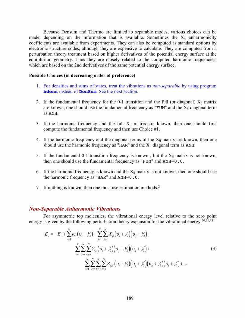
189

Because Densum and Thermo are limited to separable modes, various choices can be made, depending on the information that is available. Sometimes the Xij anharmonicity coefficients are available from experiments. They can also be computed as standard options by electronic structure codes, although they are expensive to calculate. They are computed from a perturbation theory treatment based on higher derivatives of the potential energy surface at the equilibrium geometry. Thus they are closely related to the computed harmonic frequencies, which are based on the 2nd derivatives of the same potential energy surface.

Possible Choices (in decreasing order of preference)

1. For densities and sums of states, treat the vibrations as non-separable by using program bdens instead of DenSum. See the next section.

2. If the fundamental frequency for the 0-1 transition and the full (or diagonal) Xij matrix are known, one should use the fundamental frequency as "FUN" and the Xii diagonal term as ANH.

3. If the harmonic frequency and the full Xij matrix are known, then one should first compute the fundamental frequency and then use Choice #1.

4. If the harmonic frequency and the diagonal terms of the Xij matrix are known, then one should use the harmonic frequency as "HAR" and the Xii diagonal term as ANH.

5. If the fundamental 0-1 transition frequency is known , but the Xij matrix is not known, then one should use the fundamental frequency as "FUN" and ANH=0.0.

6. If the harmonic frequency is known and the Xij matrix is not known, then one should use the harmonic frequency as "HAR" and ANH=0.0.

7. If nothing is known, then one must use estimation methods.2

Non-Separable Anharmonic Vibrations For asymmetric top molecules, the vibrational energy level relative to the zero point

energy is given by the following perturbation theory expansion for the vibrational energy:30,31,43

(3)

Ev = −Ez + ω i υi + 12( )

i=1

N

∑ + Xij υi + 12( )

j=i

N

∑i=1

N

∑ υ j + 12( ) +

Yijk υi + 12( ) υ j + 1

2( )k= j

N

∑j=i

N

∑i=1

N

∑ υk + 12( ) +

Zijkl υi + 12( )

l=k

N

∑k= j

N

∑j=i

N

∑i=1

N

∑ υ j + 12( ) υk + 1

2( ) υl + 12( ) + ...

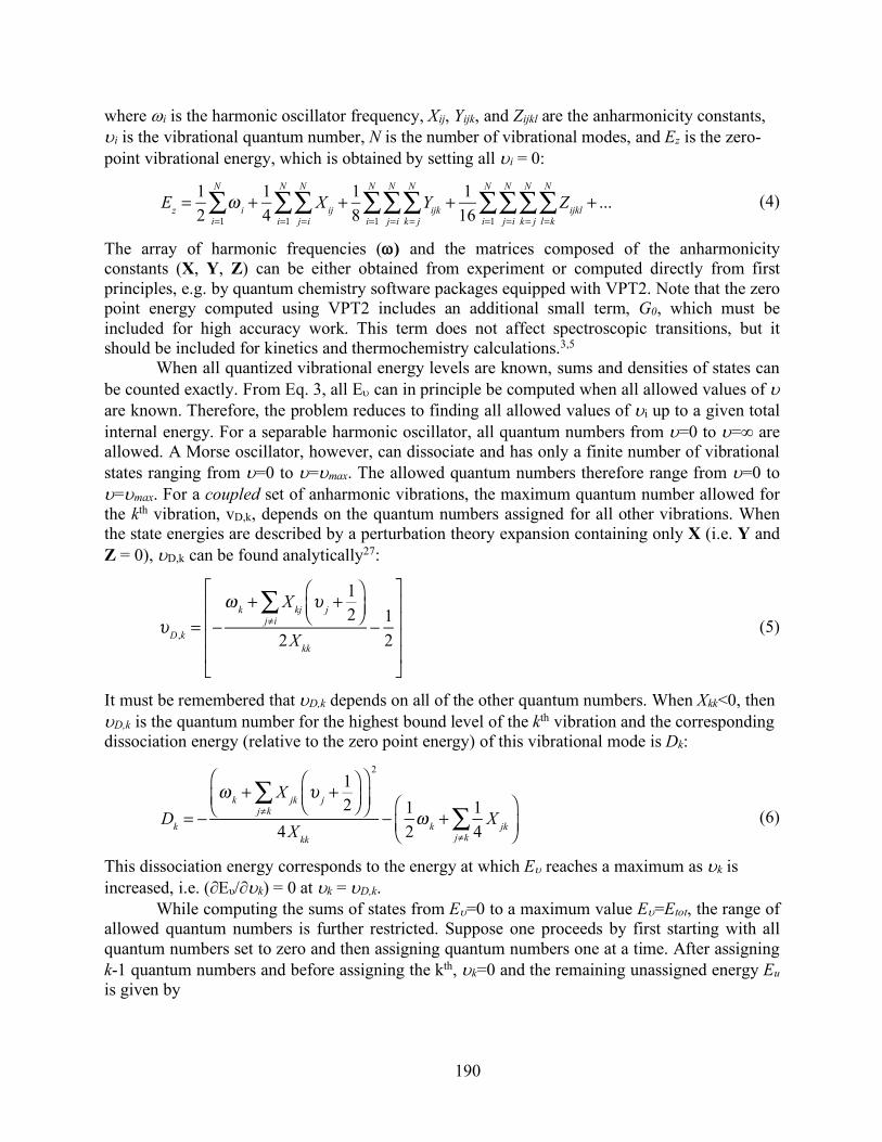
190

where wi is the harmonic oscillator frequency, Xij, Yijk, and Zijkl are the anharmonicity constants, ui is the vibrational quantum number, N is the number of vibrational modes, and Ez is the zero-point vibrational energy, which is obtained by setting all ui = 0:

(4)

The array of harmonic frequencies (w) and the matrices composed of the anharmonicity constants (X, Y, Z) can be either obtained from experiment or computed directly from first principles, e.g. by quantum chemistry software packages equipped with VPT2. Note that the zero point energy computed using VPT2 includes an additional small term, G0, which must be included for high accuracy work. This term does not affect spectroscopic transitions, but it should be included for kinetics and thermochemistry calculations.3,5

When all quantized vibrational energy levels are known, sums and densities of states can be counted exactly. From Eq. 3, all Eu can in principle be computed when all allowed values of u are known. Therefore, the problem reduces to finding all allowed values of ui up to a given total internal energy. For a separable harmonic oscillator, all quantum numbers from u=0 to u=∞ are allowed. A Morse oscillator, however, can dissociate and has only a finite number of vibrational states ranging from u=0 to u=umax. The allowed quantum numbers therefore range from u=0 to u=umax. For a coupled set of anharmonic vibrations, the maximum quantum number allowed for the kth vibration, vD,k, depends on the quantum numbers assigned for all other vibrations. When the state energies are described by a perturbation theory expansion containing only X (i.e. Y and Z = 0), uD,k can be found analytically27:

(5)

It must be remembered that uD,k depends on all of the other quantum numbers. When Xkk<0, then uD,k is the quantum number for the highest bound level of the kth vibration and the corresponding dissociation energy (relative to the zero point energy) of this vibrational mode is Dk:

(6)

This dissociation energy corresponds to the energy at which Eu reaches a maximum as uk is increased, i.e. (∂Eυ/∂uk) = 0 at uk = uD,k.

While computing the sums of states from Eu=0 to a maximum value Eu=Etot, the range of allowed quantum numbers is further restricted. Suppose one proceeds by first starting with all quantum numbers set to zero and then assigning quantum numbers one at a time. After assigning k-1 quantum numbers and before assigning the kth, uk=0 and the remaining unassigned energy Eu is given by

Ez =

12

ω ii=1

N

∑ + 14

Xijj=i

N

∑i=1

N

∑ + 18

Yijkk= j

N

∑j=i

N

∑i=1

N

∑ + 116

Zijkll=k

N

∑k= j

N

∑j=i

N

∑i=1

N

∑ + ...

υD ,k = −ω k + Xkj υ j +

12

⎛⎝⎜

⎞⎠⎟j≠i

∑2Xkk

− 12

⎡

⎣

⎢⎢⎢⎢

⎤

⎦

⎥⎥⎥⎥

Dk = −

ω k + X jk υ j +12

⎛⎝⎜

⎞⎠⎟j≠k

∑⎛

⎝⎜⎞

⎠⎟

2

4Xkk

− 12ω k +

14

X jkj≠k∑

⎛

⎝⎜⎞

⎠⎟

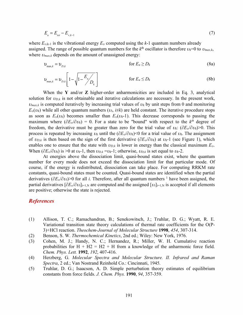
191

(7)

where Eu,k-1 is the vibrational energy Eu computed using the k-1 quantum numbers already assigned. The range of possible quantum numbers for the kth oscillator is therefore uk=0 to umax,k, where umax,k depends on the amount of unassigned energy:

for Eu ≥ Dk (8a)

for Eu ≤ Dk (8b)

When the Y and/or Z higher-order anharmonicities are included in Eq. 3, analytical solution for uD,k is not obtainable and iterative calculations are necessary. In the present work, umax,k is computed iteratively by increasing trial values of uk by unit steps from 0 and monitoring Eu(uk) while all other quantum numbers (ui, i≠k) are held constant. The iterative procedure stops as soon as Eu(uk) becomes smaller than Eu(uk-1). This decrease corresponds to passing the maximum where (∂Eu/∂uk) = 0. For a state to be "bound" with respect to the kth degree of freedom, the derivative must be greater than zero for the trial value of uk: (∂Eu/∂uk)>0. This process is repeated by increasing uk until the (∂Eu/∂uk)<0 for a trial value of uk. The assignment of uD,k is then based on the sign of the first derivative (∂Eu/∂uk) at uk-1 (see Figure 1), which enables one to ensure that the state with uD,k is lower in energy than the classical maximum Eu. When (∂Eu/∂uk) is >0 at uk-1, then uD,k =uk-1; otherwise, uD,k is set equal to uk-2.

At energies above the dissociation limit, quasi-bound states exist, where the quantum number for every mode does not exceed the dissociation limit for that particular mode. Of course, if the energy is redistributed, dissociation can take place. For computing RRKM rate constants, quasi-bound states must be counted. Quasi-bound states are identified when the partial derivatives (∂Eu/∂ui)>0 for all i. Therefore, after all quantum numbers 1 have been assigned, the partial derivatives [∂Eu/∂ui]i=1,N are computed and the assigned [ui]i=1,N is accepted if all elements are positive; otherwise the state is rejected.

References

(1) Allison, T. C.; Ramachandran, B.; Senekowitsch, J.; Truhlar, D. G.; Wyatt, R. E.

Variational transition state theory calculations of thermal rate coefficients for the O(P-3)+HCl reaction. Theochem-Journal of Molecular Structure 1998, 454, 307-314.

(2) Benson, S. W. Thermochemical Kinetics, 2nd ed.; Wiley: New York, 1976. (3) Cohen, M. J.; Handy, N. C.; Hernandez, R.; Miller, W. H. Cumulative reaction

probabilities for H + H2 = H2 + H from a knowledge of the anharmonic force field. Chem. Phys. Lett. 1992, 192, 407-416.

(4) Herzberg, G. Molecular Spectra and Molecular Structure. II. Infrared and Raman Spectra, 2 ed.; Van Nostrand Reinhold Co.: Cincinnati, 1945.


Eu = Etot − Ev ,k−1

υmax,k =υD ,k

υmax,k =υD ,k 1− 1− Eu

Dk

⎡

⎣⎢⎢

⎤

⎦⎥⎥

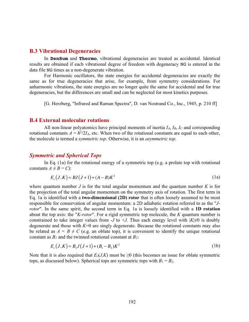
192

B.3 Vibrational Degeneracies In DenSum and Thermo, vibrational degeneracies are treated as accidental. Identical

results are obtained if each vibrational degree of freedom with degeneracy NG is entered in the data file NG times as a non-degenerate vibration.

For Harmonic oscillators, the state energies for accidental degeneracies are exactly the same as for true degeneracies that arise, for example, from symmetry considerations. For anharmonic vibrations, the state energies are no longer quite the same for accidental and for true degeneracies, but the differences are small and can be neglected for most kinetics purposes.

[G. Herzberg, "Infrared and Raman Spectra", D. van Nostrand Co., Inc., 1945, p. 210 ff]

B.4 External molecular rotations All non-linear polyatomics have principal moments of inertia IA, IB, IC and corresponding

rotational constants A = ħ2/2IA, etc. When two of the rotational constants are equal to each other, the molecule is termed a symmetric top. Otherwise, it is an asymmetric top.

Symmetric and Spherical Tops In Eq. (1a) for the rotational energy of a symmetric top (e.g. a prolate top with rotational

constants A ≠ B = C):

(1a)

where quantum number J is for the total angular momentum and the quantum number K is for the projection of the total angular momentum on the symmetry axis of rotation. The first term in Eq. 1a is identified with a two-dimensional (2D) rotor that is often loosely assumed to be most responsible for conservation of angular momentum: a 2D adiabatic rotation referred to as the "J-rotor". In the same spirit, the second term in Eq. 1a is loosely identified with a 1D rotation about the top axis: the "K-rotor". For a rigid symmetric top molecule, the K quantum number is constrained to take integer values from -J to +J. Thus each energy level with |K|≠0 is doubly degenerate and those with K=0 are singly degenerate. Because the rotational constants may also be related as A = B ≠ C (e.g. an oblate top), it is convenient to identify the unique rotational constant as B1 and the twinned rotational constant at B2:

(1b)

Note that it is also required that Er(J,K) must be ≥0 (this becomes an issue for oblate symmetric tops, as discussed below). Spherical tops are symmetric tops with B1 = B2.

Er J,K( ) = BJ J +1( ) + (A − B)K 2

Er J,K( ) = B2J J +1( ) + (B1 − B2 )K 2

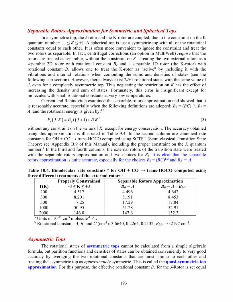
193

Separable Rotors Approximation for Symmetric and Spherical Tops In a symmetric top, the J-rotor and the K-rotor are coupled, due to the constraint on the K

quantum number: –J ≤ K ≤ +J. A spherical top is just a symmetric top with all of the rotatioinal constants equal to each other. It is often more convenient to ignore the constraint and treat the two rotors as separable. In fact, centrifugal corrections (an option in MultiWell) require that the rotors are treated as separable, without the constraint on K. Treating the two external rotors as a separable 2D rotor with rotational constant B2 and a separable 1D rotor (the K-rotor) with rotational constant B1 allows one to treat the K-rotor as "active" by including it with the vibrations and internal rotations when computing the sums and densities of states (see the following sub-section). However, there always exist 2J+1 rotational states with the same value of J, even for a completely asymmetric top. Thus neglecting the restriction on K has the effect of increasing the density and sum of states. Fortunately, this error is insignificant except for molecules with small rotational constants at very low temperatures.

Current and Rabinovitch examined the separable-rotors approximation and showed that it is reasonably accurate, especially when the following definitions are adopted: B2 = (BC)1/2, B1 = A, and the rotational energy is given by:1,2

(3)

without any constraint on the value of K, except for energy conservation. The accuracy obtained using this approximation is illustrated in Table 9.4. In the second column are canonical rate constants for OH + CO → trans-HOCO computed using SCTST (Semi-classical Transition State Theory; see Appendix B.9 of this Manual), including the proper constraint on the K quantum number.4 In the third and fourth columns, the external rotors of the transition state were treated with the separable rotors approximation and two choices for B1. It is clear that the separable rotors approximation is quite accurate, especially for the choices B2 = (BC)1/2 and B2 = A. Table 10.4. Bimolecular rate constants a for OH + CO → trans-HOCO computed using three different treatments of the external rotors b

Properly Constrained Separable Rotors Approximation T(K) -J ≤ K ≤ +J BK = A BK = A – B2D

200 4.517 4.496 4.642 300 8.201 8.191 8.453 500 17.25 17.29 17.84

1000 50.95 51.28 52.91 2000 146.0 147.6 152.3

a Units of 10-13 cm3 molecule-1 s-1. b Rotational constants A, B, and C (cm-1): 3.6640, 0.2264, 0.2132; B2D = 0.2197 cm-1.

Asymmetric Tops The rotational states of asymmetric tops cannot be calculated from a simple algebraic

formula, but partition functions and densities of states can be obtained conveniently to very good accuracy by averaging the two rotational constants that are most similar to each other and treating the asymmetric top as approximately symmetric. This is called the quasi-symmetric top approximation. For this purpose, the effective rotational constant B2 for the J-Rotor is set equal

Er J,K( ) ≈ B2J J +1( ) + B1K 2

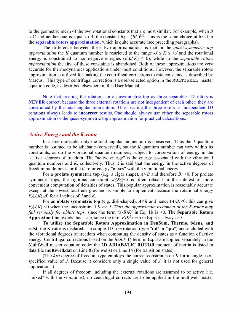
194

to the geometric mean of the two rotational constants that are most similar. For example, when B ≈ C and neither one is equal to A, the constant B2 = (BC)1/2. This is the same choice utilized in the separable rotors approximation, which is quite accurate (see preceding paragraphs).

The difference between these two approximations is that in the quasi-symmetric top approximation the K quantum number is restricted to the range -J ≤ K ≤ +J and the rotational energy is constrained to non-negaive energies (Er(J,K) ≤ 0), while in the separable rotors approximation the first of these constaints is abandoned. Both of these approximations are very accurate for thermodynamics applications under most conditions. However, the separable rotors approximation is utilized for making the centrifugal corrections to rate constants as described by Marcus.3 This type of centrifugal correction is a user-selected option in the MULTIWELL master equation code, as described elsewhere in this User Manual.

Note that treating the rotations in an asymmetric top as three separable 1D rotors is

NEVER correct, because the three external rotations are not independent of each other: they are constrained by the total angular momentum. Thus treating the three rotors as independent 1D rotations always leads to incorrect results. One should always use either the separable rotors approximation or the quasi-symmetric top approximation for practical calcualtions.

Active Energy and the K-rotor In a free molecule, only the total angular momentum is conserved. Thus the J quantum

number is assumed to be adiabatic (conserved), but the K quantum number can vary within its constraints, as do the vibrational quantum numbers, subject to conservation of energy in the "active" degrees of freedom. The "active energy" is the energy associated with the vibrational quantum numbers and K, collectively. Thus it is said that the energy in the active degrees of freedom randomizes, or the K-rotor energy "mixes" with the vibrational energy.

For a prolate symmetric top (e.g. a cigar shape), A>B and therefore B1 >0. For prolate symmetric tops, the rigorous constraint -J≤K≤+J is often relaxed in the interest of more convenient computation of densities of states. This popular approximation is reasonably accurate except at the lowest total energies and is simple to implement because the rotational energy Er(J,K) ≥0 for all values of J and K.

For an oblate symmetric top (e.g. disk-shaped), A<B and hence (A-B)<0; this can give Er(J,K) <0 when the unconstrained K >> J. Thus the approximate treatment of the K-rotor may fail seriously for oblate tops, since the term (A-B)K2 in Eq. 1b is <0. The Separable Rotors Approximation avoids this issue, since the term B1K2 term in Eq. 3 is always >0.

To utilize the Separable Rotors Approximation in DenSum, Thermo, bdens, and sctst, the K-rotor is declared as a simple 1D free rotation (type "rot" or "qro") and included with the vibrational degrees of freedom when computing the density of states as a function of active energy. Centrifugal corrections based on the B2J(J+1) term in Eq. 3 are applied separately in the MultiWell master equation code: the 2D ADIABATIC ROTOR moment of inertia is listed in data file multiwell.dat on Line 8 (for wells) or Line 14 (for transition states).

(The kro degree of freedom type employs the correct constraints on K for a single user-specified value of J. Because it considers only a single value of J, it is not used for general applications.)

If all degrees of freedom including the external rotations are assumed to be active (i.e. "mixed" with the vibrations), no centrifugal corrects are to be applied in the multiwell master

195

equation code (use the NOCENT key word) and the "top" type of degree of freedom for symmetrical tops can be utilized in densum, bdens, and sctst when calculating sums and densities of states.

References

(1) Current, J. H.; Rabinovitch, B. S. Decomposition of Chemically Activated Ethyl-d3

Radicals. Primary Intramolecular Kinetic Isotope Effect in a Nonequilibrium System. J. Chem. Phys. 1963, 38, 783-795.


(3) Marcus, R. A. Dissociation and isomerization of vibrationally excited species. III. J. Chem. Phys. 1965, 43, 2658-2661.

(4) Nguyen, T. L.; Xue, B.; Weston, R. E., Jr.; Barker, J. R.; Stanton, J. F. Reaction of HO with CO: Tunneling is Indeed Important J. Phys. Chem. Letters 2012, 3, 1549–1553; dx.doi.org/10.1021/jz300443a.

B.5 Symmetry numbers, internal rotation, and optical isomers (mirror images)

External Symmetry Numbers External symmetry numbers are based on the geometry of the chemical species).4 For use

in DenSum, MultiWell, and Thermo, we recommend the Gilbert and Smith5 convention for symmetry numbers: The external symmetry number should not contain any contribution from internal rotors and the external symmetry numbers are not used in the calculation of sums and densities of states. INTERNAL ROTOR symmetry numbers are explicitly included in the data lines for the specific internal rotors (DenSum and Thermo data files.

According to the Gilbert and Smith convention, the external symmetry number for Ethane is 3x2 = 6. The symmetry numbers for the external K-rotor and adiabatic 2-D-rotor are set equal to unity in both DenSum and Thermo. (Note that the codes are flexible enough so that other self-consistent conventions may be used instead.)

Hindered Internal Rotation Internal rotors are characterized by both the symmetry of the potential energy (i.e. the

foldedness, or number of minima (and maxima) per 2p rotation), and the symmetry of the mass distribution (or substituents) around the rotor. A potential energy surface computed using the Born-Oppenheimer approximation is independent of the masses of the nuclei. The potential energy surface for ethane internal rotation, for example, is 3-fold symmetric, but isotopic substitution can give either unsymmetrical or symmetrical mass distributions. If both the PES and the mass distribution have identical symmetries, then that is also the symmetry number of the internal rotor. It is also the number of "indistinguishable minima"; the symmetry number

196

compensates for over-counting the number of indistinguishable minima when computing the partition function:3

where σhr is the symmetry number for the hindered rotor and Ei is the ith energy eigenvalue. MultiWell has provision in Thermo and DenSum for both symmetrical and

unsymmetrical hindered internal rotations. For user convenience, the parameters for symmetrical hindered internal rotations may be entered in any one of three ways, designated by degree of freedom types "hra", "hrb", and "hrc". These types assume that the reduced internal moment of inertia is constant (independent of dihedral angle) and the potential energy of the internal rotation is given by a simple cosine function:

where U is the height of the hindrance barrier, and χ is the dihedral angle (for more complex symmetrical potentials, use type "hrd", which is discussed below). If U = 0, then the internal rotation should be modeled using a 1-D free rotor (types "rot" or "qro") with the symmetry number for the internal rotation.

Types "hra", "hrb", and "hrc" offer three convenient methods for entering the identical information. The information is identical because the harmonic frequency, hindrance barrier height, and the reduced moment of inertia for a symmetrical 1-D hindered internal rotation are related by the single equation:

where νt is the harmonic torsion frequency, U is the height of the hindrance barrier, and Ir is the reduced moment of inertia. With any two of these quantities, the third is defined. Note that this equation is only valid for σhr>1.

Unsymmetrical hindered internal rotations (σhr=1) are entered in Thermo and DenSum by designating degree of freedom type "hrd", which is a general treatment of one-dimensional hindered internal rotation. This general treatment can be used to describe internal rotation with just one well, or with two or more distinguishable wells. It can also be used for symmetrical potentials with more complicated potential energy functions. To calculate the internal rotor eigenvalues requires the potential energy function and the reduced moment of inertia (or rotational constant) as a function of dihedral angle. For an example, see the data for ClOOCl in the thermodynamics data base (directory multiwell/thermo-database/).

For convenience, three forms of the torsional potential energy are accepted by DenSum and Thermo (all coefficients in units of cm-1) for using the General hindered internal rotation treatment:

qhr =1σ hr

exp −Ei

kBT⎛⎝⎜

⎞⎠⎟i=1

∞

∑

V (χ ) = U21− cos σ hrχ( )⎡⎣ ⎤⎦

ν t =σ hr

2πU2Ir

⎛⎝⎜

⎞⎠⎟

1/2

197

Type Vhrd1

Type Vhrd2

Type Vhrd3

where χ is the dihedral angle (radians). The parameters σv (symmetry number for the potential energy: SYMMV) and φV (phase angle for the potential: PHASEV (radians)) are merely for convenience in curve-fitting.

Also for convenience, either the rotational constant or the moment of inertia, which are functions of the dihedral angle, can be entered (all coefficients in units of cm-1).

Type Bhrd1 (all coefficients in units of cm-1)

Type Ihrd1 (all coefficients in units of amu.Å2)

where χ is the dihedral angle (radians), σB and σI are symmetry numbers (SYMMM) and φB and φI are phase angles (PHASEM). It is VERY IMPORTANT that the angles are defined in the same way both for the potential and for the mass factor.

"hrd" Also Used for Symmetrical Internal Rotors. This degree of freedom type can also be used for symmetrical hindered internal rotations. The rotor symmetry number (NG) must be given, as well as coefficients for V(χ), which must have the same symmetry as the rotor symmetry number (the parameter SYMMV may equal unity or a convenient multiple of NG; it is only required that V(χ) have the correct symmetry). For an example, see the data for HONO2 in the thermodynamics data base (directory multiwell/thermo-database/).

Optical Isomers The classic example of a chemical species that has "optical isomers" (chiral stereoisomers

or mirror images) is methane substituted with four unique atoms or isotopes. There is no internal rotation in this classic example, but internal rotation can also produce optical isomers. For example, hydrogen peroxide has right-handed and left-handed forms, which are identical in all respects except for their handedness; they are mirror images of each other. The "gauche" structures of hydrocarbons may also be optical isomers. Consider the case of ethane substituted with one deuterium on each carbon: CH2D-CH2D. This molecule has three unique staggered conformers characterized by the D-C-C-D dihedral angle χ: right-handed gauche with χ = +60°, left-handed gauche with χ = -60°, and a conformer with Cs symmetry at χ = 180°. Usually (and maybe always), an internal rotation that connects optical isomers involves an unsymmetrical rotor and therefore care must be taken to treat the optical isomers and unsymmetrical hindered internal rotation in a mutually consistent fashion.

V χ( ) = Vn21− cos nσV χ +ϕV( )( )⎡⎣ ⎤⎦

n=1

N

∑

V χ( ) =V0 + Vn cos nσV χ +ϕV( )( )n=1

N

∑

V χ( ) =V0 + Vnc cos nσV χ +ϕV( )( )

n=1

N

∑ + Vns sin nσV χ +ϕV( )( )

n=1

N

∑

B χ( ) = B0 + Bn cos nσ B χ +ϕB( )( )n=1

N

∑

I χ( ) = I0 + In cos nσ I χ +ϕ I( )( )n=1

N

∑

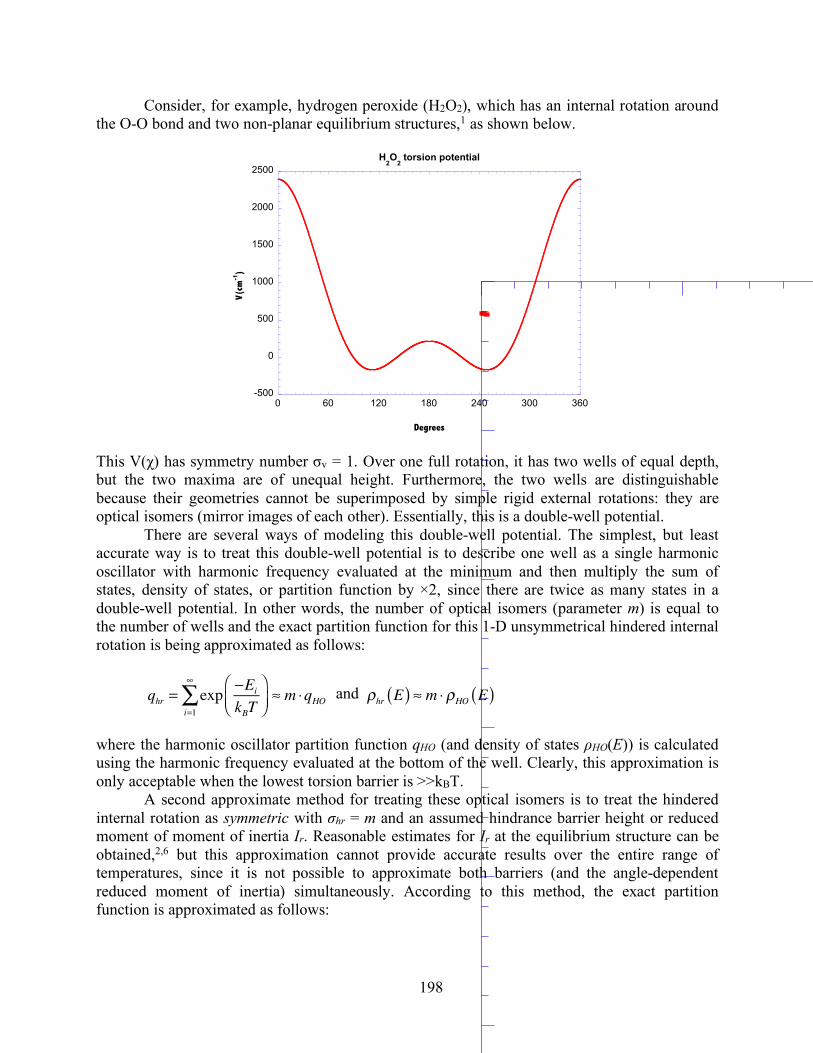
198

Consider, for example, hydrogen peroxide (H2O2), which has an internal rotation around the O-O bond and two non-planar equilibrium structures,1 as shown below.

This V(χ) has symmetry number σv = 1. Over one full rotation, it has two wells of equal depth, but the two maxima are of unequal height. Furthermore, the two wells are distinguishable because their geometries cannot be superimposed by simple rigid external rotations: they are optical isomers (mirror images of each other). Essentially, this is a double-well potential.

There are several ways of modeling this double-well potential. The simplest, but least accurate way is to treat this double-well potential is to describe one well as a single harmonic oscillator with harmonic frequency evaluated at the minimum and then multiply the sum of states, density of states, or partition function by ×2, since there are twice as many states in a double-well potential. In other words, the number of optical isomers (parameter m) is equal to the number of wells and the exact partition function for this 1-D unsymmetrical hindered internal rotation is being approximated as follows:

and

where the harmonic oscillator partition function qHO (and density of states ρHO(E)) is calculated using the harmonic frequency evaluated at the bottom of the well. Clearly, this approximation is only acceptable when the lowest torsion barrier is >>kBT.

A second approximate method for treating these optical isomers is to treat the hindered internal rotation as symmetric with σhr = m and an assumed hindrance barrier height or reduced moment of moment of inertia Ir. Reasonable estimates for Ir at the equilibrium structure can be obtained,2,6 but this approximation cannot provide accurate results over the entire range of temperatures, since it is not possible to approximate both barriers (and the angle-dependent reduced moment of inertia) simultaneously. According to this method, the exact partition function is approximated as follows:

-500

0

500

1000

1500

2000

2500

0 60 120 180 240 300 360

H2O

2 torsion potential

V(cm

-1)

Degrees

qhr = exp −Ei

kBT⎛⎝⎜

⎞⎠⎟i=1

∞

∑ ≈ m ⋅qHO ρhr E( ) ≈ m ⋅ ρHO E( )

199

where the "shr" subscript designates the symmetric hindered rotor, Ei are the exact eigenfunctions for the unsymmetrical internal rotation, and Es,i are the eigenfunctions for the symmetric rotor. Although not accurate over the entire temperature range, this approximation performs slightly better than the harmonic oscillator approach at low to intermediate temperatures.

In both of the above approximations, m (the number of optical isomers) is used as a multiplier and must be entered in the MultiWell and Thermo input files.

The most accurate approach is to calculate the eigenvalues for the double-well potential and use them directly in calculating the partition function for the hindered internal rotor. This is done by specifying the "hrd" type of degree of freedom, entering the coefficients for the angle-dependent potential energy function and angle-dependent reduced moment of inertia6 (or rotational constant). For this calculation, m must be set equal to m = 1, since the resulting partition function (and density of states) already has the requisite number of levels and should not be multiplied by an additional factor. For example, see the data for HOOH in the thermodynamics data base (directory multiwell/thermo-database/).

Of course, not all optical isomers are associated with hindered internal rotation. Those optical isomers that are not associated with a hindered rotation should still be included in m and entered in the data files.

Note that the external symmetry number is not affected by the hindered rotor treatment and is the same for any treatment of internal rotation, including a harmonic oscillator approximation. When CH2D-CH2D, HOOH, or any other unsymmetrical internal rotations are treated using the "hrd" degree of freedom type (general hindered internal rotation), then usuers should set the internal rotor symmetry to NG=1 and the number of optical isomers to m=1, but the external molecular symmetry number should simply describe the over-all molecular symmetry, which is not affected by the internal rotor treatment. Determining the external symmetry number is usually easiest for the global minimum energy conformation.

Examples

σV: Potential Symmetry

σM: Mass Symmetry

σhr: Rotor Symmetry

m: Optical Isomers

External Symmetry

CH3-CD3 3 3 3 1 3 CH3-CD2H 3 3 3 1 1 CH3-CDH2 3 3 3 1 1 CH3-CH3 3 3 3 1 6 CH2D-CH2D 3 1 1 2 2 CH2D-CD2H 3 1 1 2 1 CD3-CD3 3 3 3 1 6 HOOH 1 1 1 2 2

qhr = exp −Ei

kBT⎛⎝⎜

⎞⎠⎟i=1

∞

∑ ≈ m ⋅qshr = m ⋅ 1m

exp−Es,i

kBT⎛⎝⎜

⎞⎠⎟i=1

∞

∑⎡

⎣⎢

⎤

⎦⎥ = exp

−Es,i

kBT⎛⎝⎜

⎞⎠⎟i=1

∞

∑

ρhr E( ) ≈ m ⋅ ρshr E( )

200

CHFClBr — — — 2 1

References

(1) Dorofeeva, O. V.; Iorish, V. S.; Novikov, V. P.; Neuman, D. B. NIST-JANAF

Thermochemical Tables. II Three Molecules Related to Atmospheric Chemistry: HNO3, H2SO4, H2O2. J. Phys. Chem. Ref. Data 2003, 32, 879-901.

(2) East, A. L. L.; Radom, L. Ab initio statistical thermodynamical models for the computation of third-law entropies. J. Chem. Phys. 1997, 106, 6655-6673.

(3) Ellingson, B. A.; Lynch, V. A.; Mielke, S. L.; Truhlar, D. G. Statistical thermodynamics of bond torsional modes: Tests of separable, almost-separable, and improved Pitzer-Gwinn approximations. Journal of Chemical Physics 2006, 125.

(4) Fernández-Ramos, A.; Ellingson, B. A.; Meana-Pañeda, R.; Marques, J. M. C.; Truhlar, D. G. Symmetry numbers and chemical reaction rates. Theor. Chem. Account. 2007, 118, 813–826; DOI 10.1007/s00214-007-0328-0.



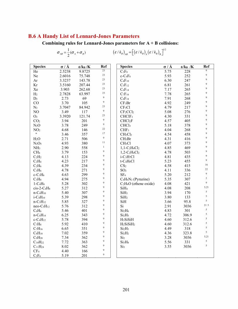
201

B.6 A Handy List of Lennard-Jones Parameters Combining rules for Lennard-Jones parameters for A + B collisions:

Species s / Å e/kB /K Ref Species s / Å e/kB /K Ref He 2.5238 9.8725 23 C3F8 5.75 228 9 Ne 2.6016 75.748 23 c-C4F8 5.93 252 9 Ar 3.3237 143.78 23 C4F10 6.30 247 9 Kr 3.5160 207.44 23 C5F12 6.81 261 9 Xe 3.903 262.68 23 C6F14 7.17 265 9 H2 2.7828 63.997 23 C7F16 7.78 265 9 D2 2.73 69 9 C8F18 7.91 268 9 CO 3.70 105 9 CF3Br 4.92 249 9 N2 3.7047 84.942 23 CF3Cl 4.79 217 9 NO 3.49 117 9 CF2CCl2 5.08 276 9 O2 3.3920 121.74 23 CHClF2 4.30 331 9 CO2 3.94 201 9 CHCl2F 4.57 405 9 N2O 3.78 249 9 CHCl3 5.18 378 9 NO2 4.68 146 22 CHF3 4.04 268 9 " 3.46 357 17 CH2Cl2 4.54 458 9 H2O 2.71 506 9 CH3Br 4.31 416 9 N2O5 4.93 380 11 CH3Cl 4.07 373 9 NH3 2.90 558 1 1,1-C2H4Cl2 4.85 469 9 CH4 3.79 153 9 1,2-C2H4Cl2 4.78 503 9 C2H2 4.13 224 9 i-C3H7Cl 4.81 435 9 C2H4 4.23 217 9 t-C4H8Cl 5.23 455 9 C2H6 4.39 234 9 CS2 4.58 415 16 C3H6 4.78 271 9 SO2 4.11 336 22 c-C3H6 4.63 299 9 SF6 5.20 212 9 C3H8 4.94 275 9 C4H4N2 (Pyrazine) 5.35 307 2 1-C4H8 5.28 302 9 C2H4O (ethene oxide) 4.08 421 9 cis-2-C4H8 5.27 312 9 SiH4 4.08 208 5,21 n-C4H10 5.40 307 9 SiH3 3.94 170 5 i-C4H10 5.39 298 9 SiH2 3.80 133 5 n-C5H12 5.85 327 9 SiH 3.66 95.8 5 neo-C5H12 5.76 312 9 Si 2.91 3036 21 5 C6H6 5.46 401 9 Si2H6 4.83 301 5 n-C6H14 6.25 343 9 Si2H5 4.72 306.9 5 c-C6H12 5.78 394 9 H3SiSiH 4.60 312.6 5 C7H8 5.92 410 9 H2SiSiH2 4.60 312.6 5 C7H16 6.65 351 9 Si2H3 4.49 318 5 C8H18 7.02 359 9 Si2H2 4.36 323.8 5 C9H20 7.34 362 9 Si2 3.28 3036 5,21 C10H22 7.72 363 9 Si3H8 5.56 331 5 C11H24 8.02 362 9 Si3 3.55 3036 5 CF4 4.40 166 9 C2F6 5.19 201 9

σ AB =12(σ A +σ B ) ε / kB( )AB = ε / kB( )A ε / kB( )B⎡⎣ ⎤⎦

1/2

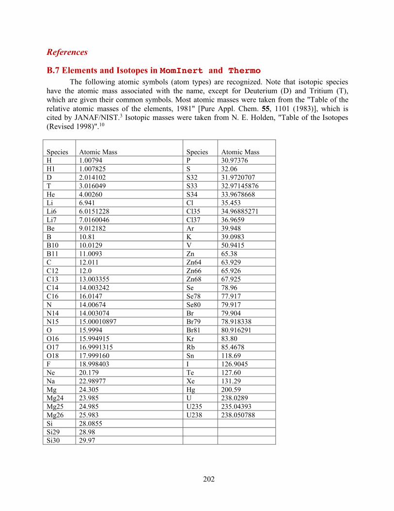
202

References

B.7 Elements and Isotopes in MomInert and Thermo The following atomic symbols (atom types) are recognized. Note that isotopic species

have the atomic mass associated with the name, except for Deuterium (D) and Tritium (T), which are given their common symbols. Most atomic masses were taken from the "Table of the relative atomic masses of the elements, 1981" [Pure Appl. Chem. 55, 1101 (1983)], which is cited by JANAF/NIST.3 Isotopic masses were taken from N. E. Holden, "Table of the Isotopes (Revised 1998)".10

Species Atomic Mass Species Atomic Mass H 1.00794 P 30.97376 H1 1.007825 S 32.06 D 2.014102 S32 31.9720707 T 3.016049 S33 32.97145876 He 4.00260 S34 33.9678668 Li 6.941 Cl 35.453 Li6 6.0151228 Cl35 34.96885271 Li7 7.0160046 Cl37 36.9659 Be 9.012182 Ar 39.948 B 10.81 K 39.0983 B10 10.0129 V 50.9415 B11 11.0093 Zn 65.38 C 12.011 Zn64 63.929 C12 12.0 Zn66 65.926 C13 13.003355 Zn68 67.925 C14 14.003242 Se 78.96 C16 16.0147 Se78 77.917 N 14.00674 Se80 79.917 N14 14.003074 Br 79.904 N15 15.00010897 Br79 78.918338 O 15.9994 Br81 80.916291 O16 15.994915 Kr 83.80 O17 16.9991315 Rb 85.4678 O18 17.999160 Sn 118.69 F 18.998403 I 126.9045 Ne 20.179 Te 127.60 Na 22.98977 Xe 131.29 Mg 24.305 Hg 200.59 Mg24 23.985 U 238.0289 Mg25 24.985 U235 235.04393 Mg26 25.983 U238 238.050788 Si 28.0855 Si29 28.98 Si30 29.97

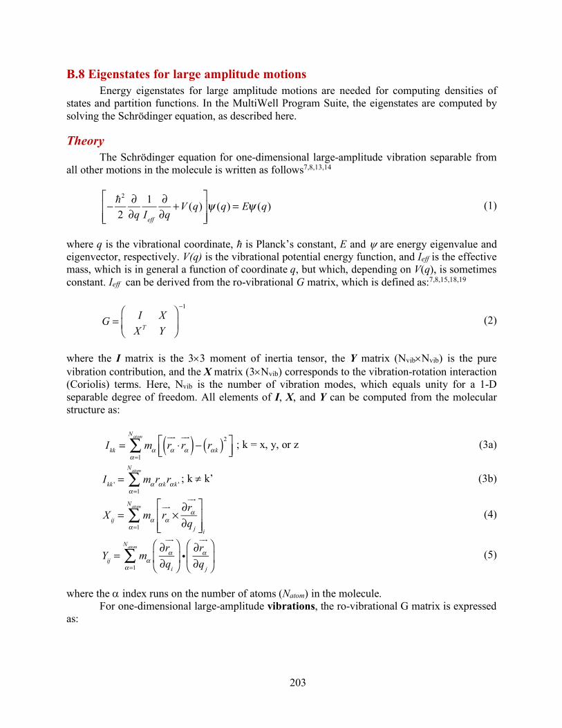
203

B.8 Eigenstates for large amplitude motions Energy eigenstates for large amplitude motions are needed for computing densities of

states and partition functions. In the MultiWell Program Suite, the eigenstates are computed by solving the Schrödinger equation, as described here.

Theory The Schrödinger equation for one-dimensional large-amplitude vibration separable from

all other motions in the molecule is written as follows7,8,13,14

(1)

where q is the vibrational coordinate, ħ is Planck’s constant, E and y are energy eigenvalue and eigenvector, respectively. V(q) is the vibrational potential energy function, and Ieff is the effective mass, which is in general a function of coordinate q, but which, depending on V(q), is sometimes constant. Ieff can be derived from the ro-vibrational G matrix, which is defined as:7,8,15,18,19

(2)

where the I matrix is the 3´3 moment of inertia tensor, the Y matrix (NvibŃvib) is the pure vibration contribution, and the X matrix (3Ńvib) corresponds to the vibration-rotation interaction (Coriolis) terms. Here, Nvib is the number of vibration modes, which equals unity for a 1-D separable degree of freedom. All elements of I, X, and Y can be computed from the molecular structure as:

; k = x, y, or z (3a)

; k ¹ k’ (3b)

(4)

(5)

where the a index runs on the number of atoms (Natom) in the molecule. For one-dimensional large-amplitude vibrations, the ro-vibrational G matrix is expressed

as:

−

2

2∂∂q

1Ieff

∂∂q

+V (q)⎡

⎣⎢⎢

⎤

⎦⎥⎥ψ (q) = Eψ (q)

G = I X

X T Y

⎛

⎝⎜⎞

⎠⎟

−1

Ikk = mα rα

⋅rα( )− rαk( )2⎡

⎣⎢⎤⎦⎥α=1

Natom

∑

Ikk ' = mαrαkrαk '

α=1

Natom

∑

Xij = mα rα

×∂rα

∂qj

⎡

⎣⎢⎢

⎤

⎦⎥⎥α=1

Natom

∑i

Yij = mα

∂rα!"

∂qi

⎛

⎝⎜

⎞

⎠⎟ i

α=1

Natom

∑ ∂rα!"

∂qj

⎛

⎝⎜

⎞

⎠⎟

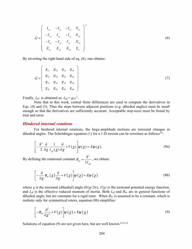
204

(6)

By inverting the right hand side of eq. (6), one obtains:

(7)

Finally, Ieff is obtained as: Ieff = g44-1. Note that in this work, central finite differences are used to compute the derivatives in

Eqs. (4) and (5). Thus the steps between adjacent positions (e.g. dihedral angles) must be small enough so that the derivatives are sufficiently accurate. Acceptable step-sizes must be found by trial and error.

Hindered internal rotations For hindered internal rotations, the large-amplitude motions are torsional changes in

dihedral angles. The Schrödinger equation (1) for a 1-D torsion can be rewritten as follows14:

. (8a)

By defining the rotational constant , we obtain:

(8b)

where χ is the torsional (dihedral) angle (0≤χ<2p), V(χ) is the torsional potential energy function, and Ieff is the effective reduced moment of inertia. Both Ieff and Bhr are in general functions of dihedral angle, but are constants for a rigid rotor. When Bhr is assumed to be a constant, which is realistic only for symmetrical rotors, equation (8b) simplifies:

(9)

Solutions of equation (9) are not given here, but are well known.4,12,14

G =

Ixx − Ixy − Ixz X11

− I yx I yy − I yz X12

− Izx − Izy Izz X13

X11 X12 X13 Y11

⎛

⎝

⎜⎜⎜⎜⎜⎜

⎞

⎠

⎟⎟⎟⎟⎟⎟

−1

G =

g11 g12 g13 g14

g21 g22 g23 g24

g31 g32 g33 g34

g41 g42 g43 g44

⎛

⎝

⎜⎜⎜⎜⎜

⎞

⎠

⎟⎟⎟⎟⎟

−

2

2∂∂χ

1Ieff (χ )

∂∂χ

+V (χ )⎡

⎣⎢⎢

⎤

⎦⎥⎥ψ (χ ) = Eψ (χ )

Bhr =

2

2Ieff

− ∂∂χ

Bhr χ( ) ∂∂χ

+V χ( )⎡

⎣⎢

⎤

⎦⎥ψ χ( ) = Eψ χ( )

−Bhr∂2

∂χ 2 +V χ( )⎡

⎣⎢

⎤

⎦⎥ψ χ( ) = Eψ χ( )

205

For the purpose of calculating densities of states and computing partition functions in the MultiWell Suite, Eq. (8b) is diagonalized to obtain energy eigenvalues, whether or not Bhr is assumed to be constant. The solutions are obtained by using the method described by Meyer.14 The Hamiltonian matrix of Eq. (8b) is given by:

(10)

where D is the matrix of the first-order derivative (∂/∂χ) operator of the internal rotation angle, DT is the transpose of D (i.e. DT(i,j) = D(j,i)), V(i,i) is the diagonal matrix of the potential energy operator, and Bhr(i,i) is the diagonal matrix element of the rotational constant; the indices are for equally spaced torsion angle grid points. For 2N +1 grid points, the elements of D are:

(11a)

for i ≠ j (11b)

To construct the symmetric matrix H, one requires both V(χ) and Bhr(χ). Several common representations of V(χ) and B(χ) (or the corresponding moment of inertia function I(χ)) can be understood by MultiWell, as explained elsewhere in this manual. The matrix H is diagonalized in order to obtain a vector of energy eigenvalues, which are convoluted with states from the other degrees of freedom to compute ro-vibrational densities of states or partition functions.

Users must supply the functions V(χ) and Bhr(χ) (or moment of inertia function I(χ)). Potential energies V(χ) and molecular geometries can be computed at discrete values of χ by obtained by using any of the many available quantum chemistry codes, such as Gaussian,6 C-Four,20, and Molpro.24. The results for V(χ) can be fitted to a suitable truncated Fourier series, and one may use codes like the I_Eckart program25 (written for use with MatLab) or LAMM program given in the MultiWell Suite to compute Bhr(χ) or Ihr(χ).

H = −DBhrD+V = DT BhrD+V

D i,i( ) = 0

D(i, j) = −1( )i− j 2sin i − j( )π / 2N −1( )⎡⎣ ⎤⎦{ }−1

206

References

(1) Barker, J. R.; Toselli, B. M. Infrared Emission Studies of the Vibrational Deactivation of Benzene Derivatives. Int. Rev. Phys. Chem. 1993, 12, 305-338.

(2) Bevilacqua, T. J.; Weisman, R. B. Collisional vibrational relaxation of a triplet state: Energy dependent energy loss from T1 pyrazine. J. Chem. Phys. 1993, 98, 6316.

(3) Chase, M. W., Jr. NIST-JANAF Thermochemical Tables. Fourth Edition. J. Phys. Chem. Ref. Data 1998, Monograph No. 9, 1-1951.

(4) Colbert, D. T.; Miller, W. H. J. Chem. Phys. 1992, 96, 1982-1991. (5) Coltrin, M. E.; Kee, R. J.; Miller, J. A. Electrochem. Soc. 1986, 133, 1206-1213. (6) Frisch, M. J.; Trucks, G. W.; Schlegel, H. B.; Scuseria, G. E.; Robb, M. A.; Cheeseman,

J. R.; Scalmani, G.; Barone, V.; Mennucci, B.; Petersson, G. A.; Nakatsuji, H.; Caricato, M.; Li, X.; Hratchian, H. P.; Izmaylov, A. F.; Bloino, J.; Zheng, G.; Sonnenberg, J. L.; Hada, M.; Ehara, M.; Toyota, K.; Fukuda, R.; Hasegawa, J.; Ishida, M.; Nakajima, T.; Honda, Y.; Kitao, O.; Nakai, H.; Vreven, T.; J. A. Montgomery, J.; Peralta, J. E.; Ogliaro, F.; Bearpark, M.; Heyd, J. J.; Brothers, E.; Kudin, K. N.; Staroverov, V. N.; Kobayashi, R.; Normand, J.; Raghavachari, K.; Rendell, A.; Burant, J. C.; Iyengar, S. S.; Tomasi, J.; Cossi, M.; Rega, N.; Millam, J. M.; Klene, M.; Knox, J. E.; Cross, J. B.; Bakken, V.; Adamo, C.; Jaramillo, J.; Gomperts, R.; Stratmann, R. E.; Yazyev, O.; Austin, A. J.; Cammi, R.; Pomelli, C.; Ochterski, J. W.; Martin, R. L.; Morokuma, K.; Zakrzewski, V. G.; Voth, G. A.; Salvador, P.; Dannenberg, J. J.; Dapprich, S.; Daniels, A. D.; Farkas, O.; Foresman, J. B.; Ortiz, J. V.; Cioslowski, J.; Fox, D. J. Gaussian 09, Revision A.1; Revision A.1 ed.; Gaussian, Inc.: Wallingford CT, 2009.

(7) Harthcock, M. A.; Laane, J. Calculation of kinetic energy terms for the vibrational Hamiltonian: Application to large-amplitude vibrations using one-, two-, and three-dimensional models. J. Mol. Spectros. 1982, 91, 300-324.

(8) Harthcock, M. A.; Laane, J. Calculation of two-dimensional vibrational potential energy surfaces utilizing prediagonalized basis sets and Van Vleck perturbation methods. J. Phys. Chem. 1985, 89, 4231–4240.

(9) Hippler, H.; Troe, J.; Wendelken, H. J. Collisional deactivation of vibrationally highly excited polyatomic molecules II. Direct observations for excited toluene. J. Chem. Phys. 1983, 78, 6709-6717.

(10) Lide, D. R. CRC Handbook of Chemistry and Physics, 81 ed.; CRC Press: Boca Raton, 2000.

(11) Makko, M. W.; Troe, J. Int. J. Chem. Kinet. 1982, 14, 399-416. (12) Marston, C. C.; Balint-Kurti, G. G. J. Chem. Phys. 1989, 91, 3571-3576. (13) Meyer, A.; Schroeder, J.; Troe, J. Photoisomerization of trans-stilbene in moderately

compressed gases: Pressure-dependent effective barriers. J. Phys. Chem. A 1999, 103, 10528-10539.

(14) Meyer, R. Trigonometric Interpolation Method for One-Dimensional Quantum-Mechanical Problems. J. Chem. Phys. 1970, 52, 2053-2059.

(15) Meyer, R.; Günthard, H. H. General Internal Motion of Molecules, Classical and Quantum-Mechanical Hamiltonian. J. Chem. Phys. 1968, 49, 1510-1520.

207

(16) Mourits, F. M.; Rummens, F. H. A. A critical evaluation of Lennard-Jones and Stockmayer potential parameters and of some correlation methods. Can. J. Chem. 1977, 55, 3007.

(17) Patrick, R.; Golden, D. M. Int. J. Chem. Kinet. 1983, 15, 1189-1227. (18) Pickett, H. M. Vibration—Rotation Interactions and the Choice of Rotating Axes for

Polyatomic Molecules. J. Chem. Phys. 1972, 56, 1715-1723. (19) Podolsky, B. Quantum-Mechanically Correct Form of Hamiltonian Function for

Conservative Systems. Phys. Rev. E 1928, 32, 812-816. (20) Stanton, J. F.; Gauss, J.; Harding, M. E.; Szalay, P. G.; Auer, w. c. f. A. A.; Bartlett, R. J.;

Benedikt, U.; Berger, C.; Bernholdt, D. E.; Bomble, Y. J.; Christiansen, O.; Heckert, M.; Heun, O.; Huber, C.; Jagan, T.-C.; Jonsson, D.; Jusélius, J.; Klein, K.; Lauderdale, W. J.; Matthews, D. A.; Metzroth, T.; O'Neill, D. P.; Price, D. R.; Prochnow, E.; Ruud, K.; Schiffmann, F.; Stopkowicz, S.; Vázquez, J.; Wang, F.; Watts, J. D. and the integral packages MOLECULE (J. Almlöf and P.R. Taylor); PROPS (P.R. Taylor); ABACUS (T. Helgaker, H.J. Aa. Jensen, P. Jørgensen, and J. Olsen); and ECP routines by A. V. Mitin and C. van Wüllen. CFOUR, a quantum chemical program package (www.cfour.de/), 2009.

(21) Svehla, R. A. NASA-TR 132, NASA 1962, (22) Troe, J. Theory of thermal unimolecular reactions at low pressures. II. Strong collision

rate constants. Applications. Journal of Chemical Physics 1977, 66, 4758-4775. (23) Weaver, A. B.; Alexeenko, A. A. J. Phys. Chem. Ref. Data 2015, 44, 023103;

http://dx.doi.org/10.1063/1.4921245. (24) Werner, H.-J.; Knowles, P. J.; Lindh, R.; Manby, F. R.; Schütz, M.; Celani, P.; Korona,

T.; Rauhut, G.; Amos, R. D.; Bernhardsson, A.; Berning, A.; Cooper, D. L.; Deegan, M. J. O.; Dobbyn, A. J.; Eckert, F.; Hampel, C.; Hetzer, G.; Lloyd, A. W.; McNicholas, S. J.; W. Meyer, W.; Mura, M. E.; Nicklass, A.; Palmieri, P.; Pitzer, R.; Schumann, U.; Stoll, H.; Stone, A. J.; Tarroni, R.; Thorsteinsson, T. MOLPRO version 2006.1 (a package of ab initio programs); version 2006.1 ed.; see http://www.molpro.net., 2006.


B.9 Semi-Classical Transition State Theory (SCTST) Much of this section was adapted from Ref. 15. Program parsctst (or older program sctst) uses a new algorithm15 developed for

computing rate constants with semi-classical transition state theory (SCTST), which was formulated by Miller and coworkers.8-11 SCTST incorporates non-separable coupling among all degrees of freedom and multi-dimensional quantum mechanical tunneling along the curved reaction path. The algorithm, which is practical for reactants containing dozens of atoms, predicts both microcanonical and canonical rate constants. In addition, the quantum chemistry code CFOUR has been extended to efficiently compute fully coupled vibrational anharmonicities for transition states at the CCSD(T) level of theory.

Semi-classical transition state theory (SCTST), has been described by W. H. Miller and coworkers.8-11 In combination with second-order vibrational perturbation theory (VPT2),12 the SCTST accounts explicitly for non-separable coupling among all degrees of freedom (including

208

the reaction coordinate) in the transition state region and multidimensional semi-classical tunneling.8,11 Miller, Handy and coworkers have shown that the SCTST thermal rate constants are in close agreement with those of full quantum dynamic calculations and experiments.5,6,11 However, the SCTST method has been limited to small reaction systems having only 3-4 atoms because of the large number of quantum states that must be computed for larger systems.5,6,11

The new computer code parsctst (or older program sctst) makes it practical to apply the theory to polyatomic reactions. The new algorithm is based on an extension of methods for computing sums and densities of states for fully-coupled anharmonic vibrations, which were described recently.13 In addition, an extension of the CFOUR electronic structure code 17 is described for computing the anharmonicity constants of transition states at the CCSD(T) level of theory. This new extension has enabled rate constant predictions based on a high level of theory.15

Theory According to the SCTST of W. H. Miller and coworkers,11 the microcanonical and

canonical rate constants are written:

(1)

(2a)

where h is Planck’s constant, kB is Boltzmann’s constant, T is the temperature, r(E) is the density of states of the reactant, Qre is the total partition function of the reactant(s), and G‡(E) is the cumulative reaction probability (CRP).9. The center of mass translations are rigorously separable. At temperatures that are not too high, it is a good approximation to treat the overall rotations as separable from the vibrations (including internal rotations), so that Eq. (2a) can be written:

(2b)

in which vibrational energy Ev is the variable of integration and the vibrational CRP is given by:

(3)

In Eq. 3, F-1 is the total number of vibrational degrees of freedom orthogonal to the reaction path. The semi-classical tunneling probability Pn is given by11

(4)

where

(5)

k(E) = 1

hG‡(E)ρ(E)

k(T ) = 1

h

G‡(E)exp(−E / kBT )dE−∞

+∞

∫Qre(T )

k(T ) = 1

hQt

‡Qr‡

QtQr

Gv‡(Ev )exp(−Ev / kBT )dEv−∞

+∞

∫Qv (T )

Gv

‡(Ev ) = ... Pn(Ev )nF−1=0∑

nF−2=0∑

n2=0∑

n1=0∑

Pn(E) = 1

1+ exp[2θ(n, E)]

θ(n, E) = −πΔE

ΩF

2

1+ 1− 4xFFΔE / ΩF2

209

(6a)

with and (7)

In these expressions, wk is the harmonic vibrational frequency, wF is the imaginary frequency of the reaction barrier, xij are the anharmonicity constants that describe coupling among the orthogonal degrees of freedom, xkF are the (pure imaginary) coupling terms between the reaction coordinate and the orthogonal degrees of freedom, and xFF is the real-valued anharmonicity constant for the reaction path, and DVo is the classical barrier height. [Note that the definition of ∆E used here and in a review article14 has the opposite sign from the definition given in the original papers; this also affects the Eq. 5.] Note that ΩF is the amplitude of the effective imaginary frequency, which is affected by coupling to all of the other vibrations (Eq. 7) and must always satisfy ΩF > 0 for acceptable states; unacceptable states are discarded. The term G0 is a constant, which is irrelevant in spectroscopic measurements (where only energy differences are important), but which must be included for thermochemistry and kinetics.5,18

For convenience, the reaction barrier height is often expressed as the difference between the zero point energy of the transition state and that of the reactant(s) (i.e. the vibrationally adiabatic ground-state potential energy difference DVaG‡), giving the following expressions:

(2c)

(6b)

(8)

and Go is incorporated into the zero-point vibrational energy of the orthogonal modes:

(9)

There are three known scenarios where SCTST/VPT2 is not sufficient.14,19 Two of these scenarios start to be come important only at extremely high and extremely low energies and temperatures. The third scenario becomes significant only at very high energies. None of these scenarios significantly affects rate constants at the temperatures that are important for most atmospheric and combustion applications.

Because the VPT2 approach is used, the SCTST/VPT2 model is subject to failures. In Eq. (5), SCTST/VPT2 will fail catastrophically when the term 1 − 4𝑥&&∆𝐸/Ω&+] becomes negative, or Ω&+ < 4𝑥&&Δ𝐸. In such a case, the quadratic equation that governs the barrier penetration integral has no physically meaningful solutions. Two possible scenarios lead to this failure: (i) First, when 𝑥&& < 0 (as is usually the case in calculations on real systems), it can happen when DE is less than Ω&+/4𝑥&& and becomes negative (DE < Ω&+/4𝑥&&< 0). This case, which corresponds to DE values being “too negative”, occurs in the deep-tunneling regime below the

ΔE = E − ΔVo −Go − ω k nk +

12

⎛⎝⎜

⎞⎠⎟k=1

F−1

∑ − xij ni +12

⎛⎝⎜

⎞⎠⎟

nj +12

⎛⎝⎜

⎞⎠⎟j=i

F−1

∑i=1

F−1

∑

ΩF =ω F − xkF nk +

12

⎛⎝⎜

⎞⎠⎟k=1

F−1

∑ ω F = −iω F xkF = ixkF

k(T ) = 1

hQt

‡Qr‡

QtQr

Gv‡(Ev )exp(−Ev / kBT )dEv−∞

+∞

∫Qv (T )

ΔE = ΔVaG‡ − E + Ev

‡

Ev

‡ = ω k nk +12

⎛⎝⎜

⎞⎠⎟k=1

F−1

∑ + xij ni +12

⎛⎝⎜

⎞⎠⎟

nj +12

⎛⎝⎜

⎞⎠⎟j=i

F−1

∑i=1

F−1

∑ − 12

ω k −14k=1

F−1

∑ xijj=i

F−1

∑i=1

F−1

∑

Ezpe = G0 +

12

ω kk=1

F−1

∑ + 14

xijj=i

F−1

∑i=1

F−1

∑

210

TS, and Wagner19 has given an extensive analysis of the problem, along with a suggested solution. When this occurs in our implementation, Pn(E) is set to zero; (ii) Second, when 𝑥&& >0 (which is very uncommon), leading to DE > Ω&+/4𝑥&&> 0. This case, which corresponds to DE values being “too positive”, can be seen in the high-energy regime above the TS. Our practical workaround to this case is to set Pn(E) to unity.

The SCTST/VPT2 approach can also experience a third type of failure. When the energy is high enough, the quantum numbers of the orthogonal degrees of freedom may be quite large. If, in addition, the off-diagonal anharmonicities (i.e., the xkF terms) that couple the reaction coordinate to the orthogonal modes are negative, ΩF may be reduced to zero, or even to negative values (see Eq. 7). Since ΩF is the effective magnitude of the imaginary frequency, a reduced value of ΩF suggests that the barrier thickness has increased and the probability of tunneling has therefore decreased. When ΩF = 0, the barrier is essentially infinite and there is no tunneling. The "negative omega" scenario (for ΩF ≤ 0) is considered to be unphysical: SCTST/VPT2 breaks down because there is no effective maximum. Possibly a higher order of vibrational perturbation theory can remedy this failure in future, but for present purposes a practical workaround is needed for the "negative omega" scenario. Our practical approach is to regard the barrier is infinitely thick if ΩF ≤ 0 and we thus assume in that case that the system behaves classically: the tunneling probability Pn = 0 when ∆E ≤ 0, and Pn = 1 when ∆E > 0.

In the next section, the new algorithm for computing the CRP is presented. For canonical (thermal) systems, Hernandez and Miller have described an efficient method for computing the rate constants directly from SCTST without the necessity for computing the CRP.8 A small modification of the new algorithm presented below can be used for this purpose, but will not be described here because we are primarily interested in computing k(E), the microcanonical rate constant, which requires the use of the CRP. However, with the CRP in hand, thermal rate constants can easily be obtained by averaging k(E) over the thermal energy distribution function. With minor extensions, the methods described here are also appropriate for computing k(E,J), the microcanonical rate constant for a specified total angular momentum quantum number J.

New Algorithm In Eqs. (1) and (2c), the CRP is obtained by summing over all states of the transition

state. When the state energies can be estimated from harmonic frequencies and anharmonicity constants, the summations in Eq. 3 can be evaluated exactly. In this "exact count" method, a realization of the vector [nk] of the vibrational quantum numbers is first determined for every quantum state of the transition state and the CRP is obtained via nested DO-loops using Eqs. (3)-(8). Such calculations are quite fast for systems with 3-4 atoms, but they become impossibly slow for systems containing more atoms. The same obstacle is encountered when computing densities of states for coupled vibrational states.13

Recently, three practical methods for computing vibrational sums and densities of states were compared.13 These included the brute force direct method, an "efficient" Monte Carlo method,1 and an extended version of the algorithm published by Basire et al.,4 which is based on the Wang-Landau algorithm.20 The extended algorithm is particularly useful for large molecular systems. As explained elsewhere,13 all three of the algorithms are based on a perturbation theory expansion of the state energies expressed as functions of the vibrational quantum numbers. (These algorithms are implemented in programs paradensum, parsctst (or older program sctst), and bdens.) A logical extension of these algorithms allows computation of the CRP.

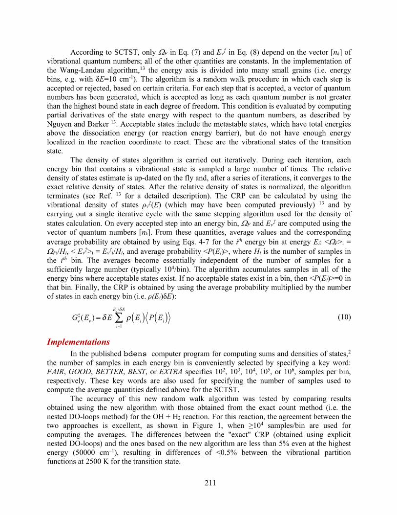
211

According to SCTST, only WF in Eq. (7) and Ev‡ in Eq. (8) depend on the vector [nk] of vibrational quantum numbers; all of the other quantities are constants. In the implementation of the Wang-Landau algorithm,13 the energy axis is divided into many small grains (i.e. energy bins, e.g. with δE=10 cm-1). The algorithm is a random walk procedure in which each step is accepted or rejected, based on certain criteria. For each step that is accepted, a vector of quantum numbers has been generated, which is accepted as long as each quantum number is not greater than the highest bound state in each degree of freedom. This condition is evaluated by computing partial derivatives of the state energy with respect to the quantum numbers, as described by Nguyen and Barker 13. Acceptable states include the metastable states, which have total energies above the dissociation energy (or reaction energy barrier), but do not have enough energy localized in the reaction coordinate to react. These are the vibrational states of the transition state.

The density of states algorithm is carried out iteratively. During each iteration, each energy bin that contains a vibrational state is sampled a large number of times. The relative density of states estimate is up-dated on the fly and, after a series of iterations, it converges to the exact relative density of states. After the relative density of states is normalized, the algorithm terminates (see Ref. 13 for a detailed description). The CRP can be calculated by using the vibrational density of states ρv‡(E) (which may have been computed previously) 13 and by carrying out a single iterative cycle with the same stepping algorithm used for the density of states calculation. On every accepted step into an energy bin, WF and Ev‡ are computed using the vector of quantum numbers [nk]. From these quantities, average values and the corresponding average probability are obtained by using Eqs. 4-7 for the ith energy bin at energy Ei: <WF>i = WFi/Hi, < Ev‡>i = Ev‡i/Hi, and average probability <P(Ei)>, where Hi is the number of samples in the ith bin. The averages become essentially independent of the number of samples for a sufficiently large number (typically 104/bin). The algorithm accumulates samples in all of the energy bins where acceptable states exist. If no acceptable states exist in a bin, then <P(Ei)>=0 in that bin. Finally, the CRP is obtained by using the average probability multiplied by the number of states in each energy bin (i.e. ρ(Ei)δE):

(10)

Implementations In the published bdens computer program for computing sums and densities of states,2

the number of samples in each energy bin is conveniently selected by specifying a key word: FAIR, GOOD, BETTER, BEST, or EXTRA specifies 102, 103, 104, 105, or 106, samples per bin, respectively. These key words are also used for specifying the number of samples used to compute the average quantities defined above for the SCTST.

The accuracy of this new random walk algorithm was tested by comparing results obtained using the new algorithm with those obtained from the exact count method (i.e. the nested DO-loops method) for the OH + H2 reaction. For this reaction, the agreement between the two approaches is excellent, as shown in Figure 1, when ≥104 samples/bin are used for computing the averages. The differences between the "exact" CRP (obtained using explicit nested DO-loops) and the ones based on the new algorithm are less than 5% even at the highest energy (50000 cm–1), resulting in differences of <0.5% between the vibrational partition functions at 2500 K for the transition state.

Gv

‡(Ev ) = δ E ρ Ei( ) P Ei( )i=1

Ev /δ E

∑

212

Program parsctst (Section 8.4; or older program sctst, Section 8.3) generates a supplementary data filed named <name>.qcrp, which is required when using program Thermo to compute thermal rate constants using the SCTST. This data file contains the partition function corresponding to the CRP.

(11)

where ρ‡v(Ev) is the derivative of G‡v(Ev) with respect to Ev. The integral on the right hand side of Eq. 11 is needed for Eq. 2c. The expression for Q‡v(T) is more convenient for use with program Thermo.

VPT2/CCSD(T) for Transition States All of the harmonic vibrational frequencies and xij anharmonicity coefficients can be

obtained for stable species from first principles by using second order vibrational perturbation theory (VPT2), which has been implemented for stable molecules in quantum chemical software packages such as GAUSSIAN 7 and CFOUR 17. The anharmonicity coefficients are obtained from the full cubic force field together with the semi-diagonal quartic force field, which can be computed by finite differences from the analytic first and second derivatives 3,17. For highly accurate methods such as CCSD(T), analytic second derivatives are only available in CFOUR 17. For this work, VPT2 computation of the anharmonicities was implemented for transition states at the CCSD(T) level of theory in CFOUR. Whenever Fermi resonances are detected, deperturbation was applied using a criterion of 100 cm-1 for the frequency difference. The combination of the new algorithm for the SCTST and implementation of VPT2 for transition states constitutes an effective tool for computing the CRP and/or thermal rate constants from first principles with high accuracy.

Reaction Critical Energy In the absence of quantum mechanical tunneling, the critical energy E0 for a unimolecular

reaction (or a bimolecular reaction according to microcanonical TST) is the difference between the enthalpies at 0 K of the transition state and the reactant(s):

E0 = ∆fHTS(0) - ∆fHreac(0) (12) This definition of the reaction critical energy is not appropriate when quantum

mechanical tunneling occurs, because tunneling takes place at lower energies. Tunneling occurs whenever the energy is below the top of the barrier (i.e. E < E0, where E0 is defined as above) but above that of the zero point energy of the product. Thus when tunneling is included the appropriate value to be utilized for "E0" depends on whether the reaction is endothermic or exothermic (including zero point energy corrections), regardless of the reaction barrier height.

In the MultiWell master equation code, the critical energy is defined as in Eq. 12 even when tunneling through an Eckart barrier is invoked (keyword 'tun' on Line 14 in the multiwell.dat data file), because the reactant and product enthalpies are employed automatically to account for tunneling below the top of the barrier. When using an external file containing the CRP generated by Program sctst, this step is NOT automated and the user must enter the value for critical energy obtained from the following:

Endothermic reactions: E0 = ∆fHprod(0) - ∆fHreac(0) (13a)

Qv

‡ T( ) = ρv‡(Ev )exp(−Ev / kBT )dEv0

+∞

∫ = kBT( )−1Gv

‡(Ev )exp(−Ev / kBT )dEv0

+∞

∫

213

Exothermic reactions: E0 = 0 (13b)

(Note: the keyword 'tun' only applies to tunneling through an Eckart barrier and must NOT be employed when using the CRP, since tunneling is already included in the CRP.)

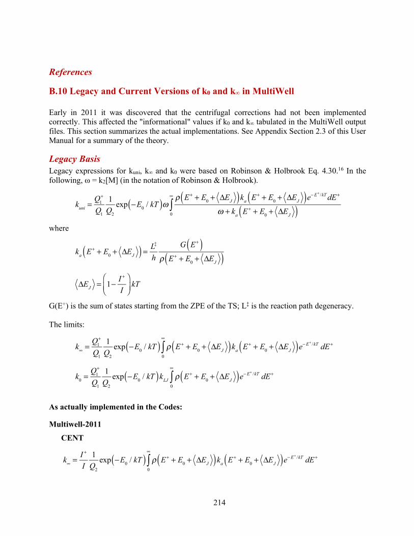
214

References

B.10 Legacy and Current Versions of k0 and k∞ in MultiWell Early in 2011 it was discovered that the centrifugal corrections had not been implemented correctly. This affected the "informational" values if k0 and k∞ tabulated in the MultiWell output files. This section summarizes the actual implementations. See Appendix Section 2.3 of this User Manual for a summary of the theory.

Legacy Basis Legacy expressions for kuni, k∞ and k0 were based on Robinson & Holbrook Eq. 4.30.16 In the following, ω = k2[M] (in the notation of Robinson & Holbrook).

where

G(E+) is the sum of states starting from the ZPE of the TS; L‡ is the reaction path degeneracy. The limits:

As actually implemented in the Codes:

Multiwell-2011

CENT

kuni =

Q1+

Q1

1Q2

exp −E0 / kT( )ω ρ E+ + E0 + ΔEJ( )ka E+ + E0 + ΔEJ( )e−E+ /kT dE+

ω + ka E+ + E0 + ΔEJ( )0

∞

∫

ka E+ + E0 + ΔEJ( ) = L‡

hG E+( )

ρ E+ + E0 + ΔEJ( )

ΔEJ = 1− I +

I⎛⎝⎜

⎞⎠⎟

kT

k∞ =

Q1+

Q1

1Q2

exp −E0 / kT( ) ρ E+ + E0 + ΔEJ( )ka E+ + E0 + ΔEJ( )e−E+ /kT dE+

0

∞

∫

k0 =

Q1+

Q1

1Q2

exp −E0 / kT( )kLJ ρ E+ + E0 + ΔEJ( )e−E+ /kT dE+

0

∞

∫

k∞ = I +

I1

Q2

exp −E0 / kT( ) ρ E+ + E0 + ΔEJ( )ka E+ + E0 + ΔEJ( )e−E+ /kT dE+

0

∞

∫

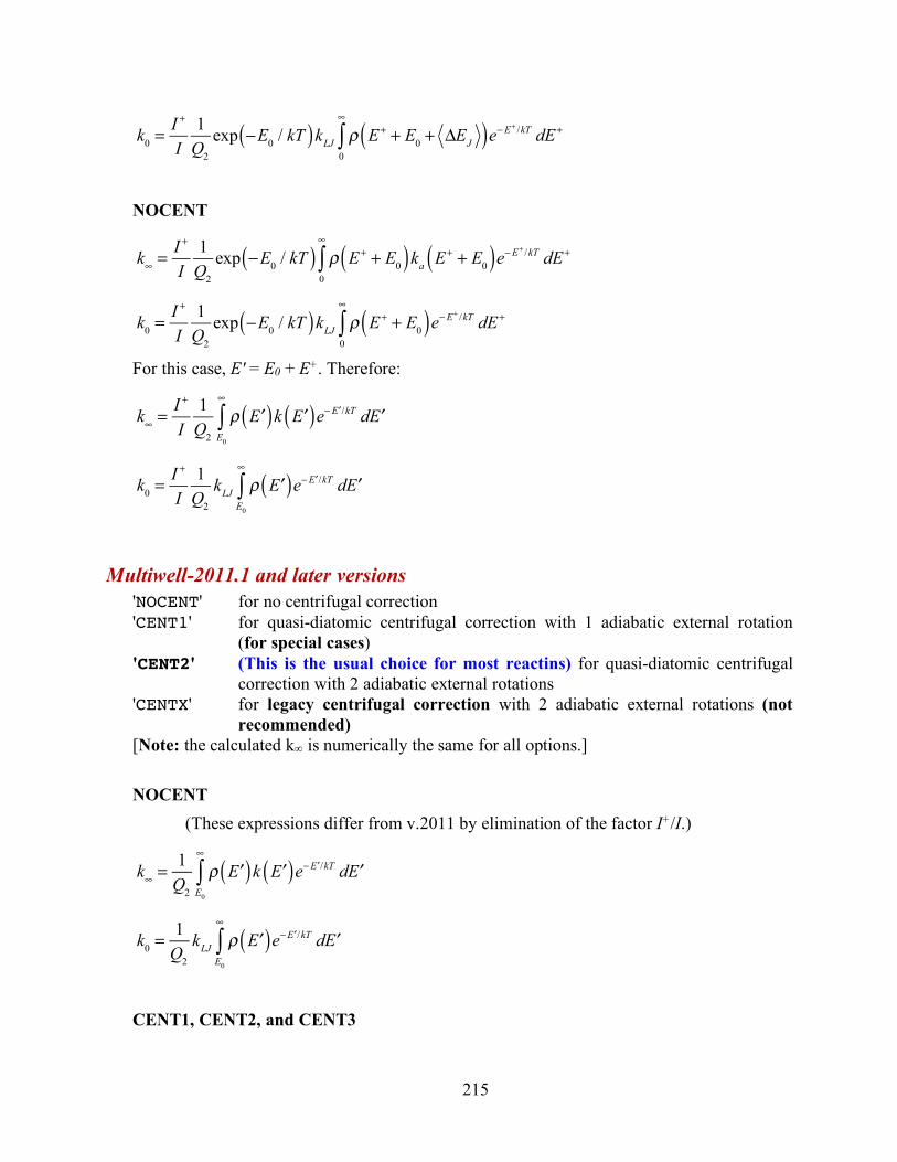
215

NOCENT

For this case, E' = E0 + E+. Therefore:

Multiwell-2011.1 and later versions 'NOCENT' for no centrifugal correction 'CENT1' for quasi-diatomic centrifugal correction with 1 adiabatic external rotation

(for special cases) 'CENT2' (This is the usual choice for most reactins) for quasi-diatomic centrifugal

correction with 2 adiabatic external rotations 'CENTX' for legacy centrifugal correction with 2 adiabatic external rotations (not

recommended) [Note: the calculated k∞ is numerically the same for all options.]

NOCENT (These expressions differ from v.2011 by elimination of the factor I+/I.)

CENT1, CENT2, and CENT3

k0 =

I +

I1

Q2

exp −E0 / kT( )kLJ ρ E+ + E0 + ΔEJ( )e−E+ /kT dE+

0

∞

∫

k∞ = I +

I1

Q2

exp −E0 / kT( ) ρ E+ + E0( )ka E+ + E0( )e−E+ /kT dE+

0

∞

∫

k0 =

I +

I1

Q2

exp −E0 / kT( )kLJ ρ E+ + E0( )e−E+ /kT dE+

0

∞

∫

k∞ = I +

I1

Q2

ρ ′E( )k ′E( )e− ′E /kT d ′EE0

∞

∫

k0 =

I +

I1

Q2

kLJ ρ ′E( )e− ′E /kT d ′EE0

∞

∫

k∞ = 1

Q2

ρ ′E( )k ′E( )e− ′E /kT d ′EE0

∞

∫

k0 =

1Q2

kLJ ρ ′E( )e− ′E /kT d ′EE0

∞

∫

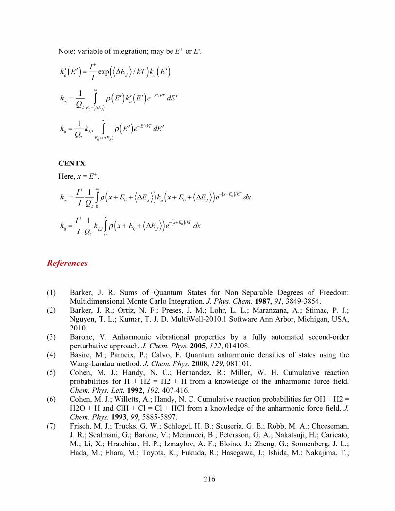
216

Note: variable of integration; may be E+ or E'.

CENTX Here, x = E+.

References


(2) Barker, J. R.; Ortiz, N. F.; Preses, J. M.; Lohr, L. L.; Maranzana, A.; Stimac, P. J.; Nguyen, T. L.; Kumar, T. J. D. MultiWell-2010.1 Software Ann Arbor, Michigan, USA, 2010.

(3) Barone, V. Anharmonic vibrational properties by a fully automated second-order perturbative approach. J. Chem. Phys. 2005, 122, 014108.

(4) Basire, M.; Parneix, P.; Calvo, F. Quantum anharmonic densities of states using the Wang-Landau method. J. Chem. Phys. 2008, 129, 081101.

(5) Cohen, M. J.; Handy, N. C.; Hernandez, R.; Miller, W. H. Cumulative reaction probabilities for H + H2 = H2 + H from a knowledge of the anharmonic force field. Chem. Phys. Lett. 1992, 192, 407-416.

(6) Cohen, M. J.; Willetts, A.; Handy, N. C. Cumulative reaction probabilities for OH + H2 = H2O + H and ClH + Cl = Cl + HCl from a knowledge of the anharmonic force field. J. Chem. Phys. 1993, 99, 5885-5897.

(7) Frisch, M. J.; Trucks, G. W.; Schlegel, H. B.; Scuseria, G. E.; Robb, M. A.; Cheeseman, J. R.; Scalmani, G.; Barone, V.; Mennucci, B.; Petersson, G. A.; Nakatsuji, H.; Caricato, M.; Li, X.; Hratchian, H. P.; Izmaylov, A. F.; Bloino, J.; Zheng, G.; Sonnenberg, J. L.; Hada, M.; Ehara, M.; Toyota, K.; Fukuda, R.; Hasegawa, J.; Ishida, M.; Nakajima, T.;

′ka ′E( ) = I +

Iexp ΔEJ / kT( )ka ′E( )

k∞ = 1

Q2

ρ ′E( ) ′ka ′E( )e− ′E /kT d ′EE0+ ΔEJ

∞

∫

k0 =

1Q2

kLJ ρ ′E( )e− ′E /kT d ′EE0+ ΔEJ

∞

∫

k∞ = I +

I1

Q2

ρ x + E0 + ΔEJ( )ka x + E0 + ΔEJ( )e− x+E0( )/kT dx0

∞

∫

k0 =

I +

I1

Q2

kLJ ρ x + E0 + ΔEJ( )e− x+E0( )/kT dx0

∞

∫

217

Honda, Y.; Kitao, O.; Nakai, H.; Vreven, T.; J. A. Montgomery, J.; Peralta, J. E.; Ogliaro, F.; Bearpark, M.; Heyd, J. J.; Brothers, E.; Kudin, K. N.; Staroverov, V. N.; Kobayashi, R.; Normand, J.; Raghavachari, K.; Rendell, A.; Burant, J. C.; Iyengar, S. S.; Tomasi, J.; Cossi, M.; Rega, N.; Millam, J. M.; Klene, M.; Knox, J. E.; Cross, J. B.; Bakken, V.; Adamo, C.; Jaramillo, J.; Gomperts, R.; Stratmann, R. E.; Yazyev, O.; Austin, A. J.; Cammi, R.; Pomelli, C.; Ochterski, J. W.; Martin, R. L.; Morokuma, K.; Zakrzewski, V. G.; Voth, G. A.; Salvador, P.; Dannenberg, J. J.; Dapprich, S.; Daniels, A. D.; Farkas, O.; Foresman, J. B.; Ortiz, J. V.; Cioslowski, J.; Fox, D. J. Gaussian 09, Revision A.1; Revision A.1 ed.; Gaussian, Inc.: Wallingford CT, 2009.




(11) Miller, W. H.; Hernandez, R.; Handy, N. C.; Jayatilaka, D.; Willetts, A. Ab initio Calculation of Anharmonic Constants for a Transition-State, with Application to Semiclassical Transition-State Tunneling Probabilities. Chemical Physics Letters 1990, 172, 62-68; Doi 10.1016/0009-2614(90)87217-F.

(12) Mills, I. M. Vibration-Rotation Structure in Asymmetric- and Symmetric-Top Molecules. In Molecular Spectroscopy: Modern Research; Rao, K. N., Mathews, C. W., Eds.; Academic Press: New York, 1972; Vol. 1; pp 115-140.


(14) Nguyen, T. L.; Barker, J. R.; Stanton, J. F. Atmospheric Reaction Rate Constants and Kinetic Isotope Effects Computed Using the HEAT Protocol and Semi-Classical Transition State Theory. In Advances in Atmospheric Chemistry; Barker, J. R., Steiner, A. L., Wallington, T. J., Eds.; World Scientific: Singapore, 2017; Vol. 1; pp 403-492.



(17) Stanton, J. F.; Gauss, J.; Harding, M. E.; Szalay, P. G.; Auer, w. c. f. A. A.; Bartlett, R. J.; Benedikt, U.; Berger, C.; Bernholdt, D. E.; Bomble, Y. J.; Christiansen, O.; Heckert, M.; Heun, O.; Huber, C.; Jagan, T.-C.; Jonsson, D.; Jusélius, J.; Klein, K.; Lauderdale, W. J.; Matthews, D. A.; Metzroth, T.; O'Neill, D. P.; Price, D. R.; Prochnow, E.; Ruud, K.; Schiffmann, F.; Stopkowicz, S.; Vázquez, J.; Wang, F.; Watts, J. D. and the integral packages MOLECULE (J. Almlöf and P.R. Taylor); PROPS (P.R. Taylor); ABACUS (T. Helgaker, H.J. Aa. Jensen, P. Jørgensen, and J. Olsen); and ECP routines by A. V. Mitin and C. van Wüllen. CFOUR, a quantum chemical program package (www.cfour.de/), 2009.


218

(19) Wagner, A. F. Improved Multidimensional Semiclassical Tunneling Theory. J. Phys. Chem. A 2013, 117, 13089−13100; dx.doi.org/10.1021/jp409720s.

(20) Wang, F.; Landau, D. P. Efficient, Multiple-Range Random Walk Algorithm to Calculate the Density of States. Phys. Rev. Letters 2001, 86, 2050-2053.

219

Appendix C. How to … This section outlines how to carry out various tasks needed by many users. It is under

development and more sections will be added in future releases of this User Manual.

C.1 How to set up the double arrays in MultiWell The double arrays consist of two arrays in one. The lower energy portion ranges in

energy from E = 0 up to Emax1; the upper energy portion ranges in energy from E = 0 up to Emax2. The total size of the double array is Isize and the number of "energy grains" (i.e. energy bins) in the lower and upper parts of the double array are Imax1 and Imax2, respectively, and the respective energy grain sizes are Egrain1 and Egrain2. The relationships among these quantities are as follows:

Emax1 = (Imax1-1)*Egrain1 Emax2 = (Imax2-1)*Egrain2

Isize = Imax1 + Imax2 To set up double arrays, users must specify Egrain1, Imax1, Emax2, and Isize; the

remaining parameters are determined by the program from the relationships given above. The following guidelines are useful for deciding on the values for the parameters.

Egrain1

• Should be small enough so that further reductions in its size do not significantly affect the numerical results (i.e. it should achieve numerical convergence).

• Should be ~10% of kBT, or less (for good accuracy in computing k∞). • Should not be too small, since that adds a computational burden. • Typical choices: 5 or 10 cm-1 (usually 10 cm-1).

Imax1 • Should be large enough so that the density of states in adjacent energy grains near

Emax1 differ by less than 5%. DenSum will give a warning if the grain-to-grain fluctuations are too large.

• Typically, Imax should be large enough so that Emax1 is greater than the highest vibrational wavenumber (typically greater than ~3000 cm-1).

• Typical choice: 400 (for Egrain1 = 10 cm-1). Emax2

• Should be high enough so that none of the stochastic trials attempt to reach a higher energy. If that occurs, MultiWell execution will halt and a Fatal Error will be reported.

• Typical choices: 50000 cm-1 for T ≤300 K; 85000 cm-1 for T≤3000 K. Isize

• Should be chosen large enough so that Egrain2 ≤ kBT/2 (for good convergence on the numerical computation of k∞).

• Typical choices: 1000 for simulations at 300 K, 1500 for very high temperatures.

220

C.2 How to test the double-array parameters in MultiWell In principle, it is wise to test your choices of parameters to determine whether the

calculations are reaching numerical convergence. In other words, one should determine whether the choices of Egrain1 and Egrain2 are small enough and that Emax1 and Emax2 are high enough.

The tests are carried out on a small subset of representative simulations with pressures and temperatures at the middle and at the extremes of their ranges, for a total of nine simulations. For narrow pressure ranges and temperature ranges, only one representative set of conditions may be necessary. Thus the amount of testing depends on the system and on experience with similar simulations.

Numerical convergence has been achieved when the grain sizes are small enough and the maximum energies are high enough so that further grain size reductions and/or further maximum energy increases do not result in significant differences in the calculations.

The most important measure of convergence is to ascertain whether the fractional yields computed for the same simulated time duration are independent of the grain size.

Two additional key quantities affected by grain size and maximum energy are kinf and kosc (i.e. the high pressure limit k∞ and the low pressure limit k0), which are printed by MultiWell for information purposes in the table summarizing transition state and reaction properties (preceding the table summarizing the stochastic simulations). These rate constants are not actually used by MultiWell in the simulations, but they are useful to users. The value for k∞ should agree within a few percent with the corresponding canonical rate constant calculated by Thermo with the same input parameters.

C.3 How estimate Lennard-Jones and energy transfer parameters It is very difficult to compute proper energy transfer parameters. Instead, they are usually

obtained by fitting experimental rate constant data. There are two parts to the problem: obtaining Lennard-Jones (LJ) parameters and estimating energy transfer parameter α for the exponential-down model, which is recommended for most purposes.

The LJ parameters can be estimated by using the critical properties of the compound, which may in turn be estimated using various empirical correlations. However, it is almost always sufficiently accurate to estimate the parameters, based on analogy. A table of LJ parameters can be found in Appendix B.6 of this User Manual.

Experience shows that parameter α in the exponential model (i.e. a single component of the bi-exponential model) usually is in the range from 100 cm-1 to 1000 cm-1; 250 cm-1 is a good first guess.

Experimental rate constant data can be fitted by varying the value of parameter α until a good fit has been achieved. It is efficient to start by computing results for several values of α that cover the whole range expected (typically 100, 250, 500, and 1000 cm-1). For most molecular species, the "true" value is probably somewhere in this range. By examining a plot of the data superimposed on a plot of this family of simulations, it will be possible to get a better estimate of the fitted value. The plot will also demonstrate the sensitivity of the simulations to the assumed value.

221

C.4 How to obtain rate constants from MultiWell simulations Master equation simulations are accurate at all time-scales over which statistical rate

theory is valid, but "rate constants" are valid only after an initial energy relaxation has been completed. When simulating experiments (in which intermediates might never be thermalized), it is not necessary to define rate constants. In that case, the master equation results are employed directly. However, master equations are also used to compute rate constants for predictions and for comparisons with experimental values.

MultiWell does not calculate conventional reaction rate constants directly; the output must be analyzed further. The data from the simulation can be analyzed by using least squares fitting and other techniques, just as is done in analyzing experiments.1,6,8,11,13,15,16 In the following, several pragmatic approaches are described.

Single-well Unimolecular Reactions Single-well reaction systems may have multiple channels and all of the reaction channels

are irreversible unimolecular reactions in multiwell simulations. To find kuni in the pressure fall-off regime, you need to carry out simulations at the temperature and pressure of interest. Then, you can find kuni in one of two ways (outlined below), both of which depend on the population distribution reaching STEADY STATE. The population distribution will approach steady-state after an initial transient period if the reaction rates are slower than the energy relaxation rates. As the population distributions approach steady state, the average vibrational energy of the system (Evib in output file multiwell.out) and the reaction flux coefficients (in output file multiwell.rates) will asymptotically approach constant values. Due to the stochastic simulation noise that accompanies stochastic simulations, these values will usually display fluctuations.

Here are the two methods for finding unimolecular rate constants: a) Reaction Flux Coefficients: the output file 'multiwell.rate' gives reaction flux

coefficients for all the reactions, based on the instantaneous population distributions and on k(E) for each reaction. When the population distribution in the well is AT STEADY STATE, the flux coefficient for each irreversible channel is equal to kuni for that channel; the total kuni is equal to the sum of the channel-specific rate constants. To use this feature, however, requires many, many stochastic trials in a single simulation in order to reduce the stochastic sampling noise. This technique should not be used for multi-well reaction systems, because the reactions are reversible and the unimolecular rate constants therefore depend algebraically on more than one reaction flux coefficient.

b) Curve fitting: the decay of population in a SINGLE-WELL reaction is exponential with total rate constant kuni, which may obtained from a semi-log plot: natural logarithm of population ("fraction") vs. time; the slope of the plot is equal to -kuni. For multi-channel reactions, the branching ratios of the individual channels can be obtained from the relative rates of producing products or relative product yields ("fractions"), evaluated for the period over which the population is in steady-state.

It is important to note that if the analysis requires time periods longer than needed for more than a few thousand collisions, the simulations become very time-consuming. MultiWell is not designed for computing slow, steady-state unimolecular reactions. The factors affecting computation time are discussed in the following sub-section.

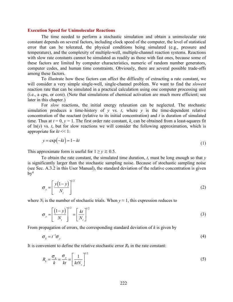
222

Execution Speed for Unimolecular Reactions The time needed to perform a stochastic simulation and obtain a unimolecular rate

constant depends on several factors, including clock speed of the computer, the level of statistical error that can be tolerated, the physical conditions being simulated (e.g., pressure and temperature), and the complexity of multiple-well, multiple-channel reaction systems. Reactions with slow rate constants cannot be simulated as readily as those with fast ones, because some of these factors are limited by computer characteristics, numeric of random number generators, computer codes, and human time constraints. Obviously, there are several possible trade-offs among these factors.

To illustrate how these factors can affect the difficulty of extracting a rate constant, we will consider a very simple single-well, single-channel problem. We want to find the slowest reaction rate that can be simulated in a practical calculation using one computer processing unit (i.e., a cpu, or core). (Note that simulations of chemical activation are much more efficient; see later in this chapter.)

For slow reactions, the initial energy relaxation can be neglected. The stochastic simulation produces a time-history of y vs. t, where y is the time-dependent relative concentration of the reactant (relative to its initial concentration) and t is duration of simulated time. Thus at t = 0, y = 1. The first order rate constant, k, can be obtained from a least-squares fit of ln(y) vs. t, but for slow reactions we will consider the following approximation, which is appropriate for kt << 1:

(1)

This approximate form is useful for 1 ≥ y ≳ 0.5. To obtain the rate constant, the simulated time duration, t, must be long enough so that y

is significantly larger than the stochastic sampling noise. Because of stochastic sampling noise (see Sec. A.3.2 in this User Manual), the standard deviation of the relative concentration is given by4

(2)

where Nt is the number of stochastic trials. When y ≈ 1, this expression reduces to

(3)

From propagation of errors, the corresponding standard deviation of k is given by

(4)

It is convenient to define the relative stochastic error Rk in the rate constant:

(5)

y = exp −kt( ) ≈1− kt

σ y =

y 1− y( )Nt

⎡

⎣⎢⎢

⎤

⎦⎥⎥

1/2

σ y ≈

1− y( )Nt

⎡

⎣⎢⎢

⎤

⎦⎥⎥

1/2

= ktNt

⎡

⎣⎢

⎤

⎦⎥

1/2

σ k = t−1σ y

Rk =

σ k

k=σ y

kt= 1

ktNt

⎡

⎣⎢

⎤

⎦⎥

1/2

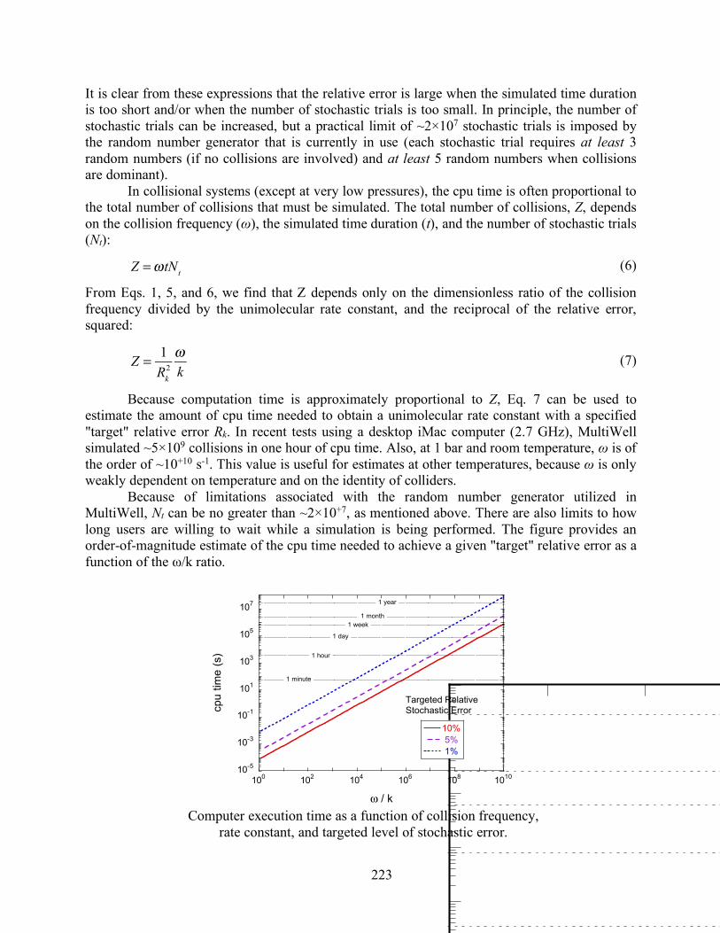
223

It is clear from these expressions that the relative error is large when the simulated time duration is too short and/or when the number of stochastic trials is too small. In principle, the number of stochastic trials can be increased, but a practical limit of ~2×107 stochastic trials is imposed by the random number generator that is currently in use (each stochastic trial requires at least 3 random numbers (if no collisions are involved) and at least 5 random numbers when collisions are dominant).

In collisional systems (except at very low pressures), the cpu time is often proportional to the total number of collisions that must be simulated. The total number of collisions, Z, depends on the collision frequency (ω), the simulated time duration (t), and the number of stochastic trials (Nt):

(6)

From Eqs. 1, 5, and 6, we find that Z depends only on the dimensionless ratio of the collision frequency divided by the unimolecular rate constant, and the reciprocal of the relative error, squared:

(7)

Because computation time is approximately proportional to Z, Eq. 7 can be used to estimate the amount of cpu time needed to obtain a unimolecular rate constant with a specified "target" relative error Rk. In recent tests using a desktop iMac computer (2.7 GHz), MultiWell simulated ~5×109 collisions in one hour of cpu time. Also, at 1 bar and room temperature, ω is of the order of ~10+10 s-1. This value is useful for estimates at other temperatures, because ω is only weakly dependent on temperature and on the identity of colliders.

Because of limitations associated with the random number generator utilized in MultiWell, Nt can be no greater than ~2×10+7, as mentioned above. There are also limits to how long users are willing to wait while a simulation is being performed. The figure provides an order-of-magnitude estimate of the cpu time needed to achieve a given "target" relative error as a function of the ω/k ratio.

Computer execution time as a function of collision frequency,

rate constant, and targeted level of stochastic error.

Z =ωtNt

Z = 1

Rk2

ωk

10-5

10-3

10-1

101

103

105

107

100 102 104 106 108 1010

10% 5% 1%

cpu

time

(s)

ω / k

Targeted Relative Stochastic Error

1 hour

1 day

1 week 1 month

1 minute

1 year

224

From the figure, it is clear that "slow reactions" (i.e., slow compared to collision

frequency) require long simulation times in order to achieve small relative stochastic errors. Obviously, very long simulations can be performed. In our research, we sometimes run simulations that require ~24 hrs of wall-clock time, but rarely longer than that. Stochastic simulations are best suited to cases where the pressure (and thus the collision frequency ω) is small and the rate constant is large. At very low pressures, the cpu times reach a small but finite lower limit (due to computational overhead) that is not described by Eq. 7.

Multiple-Well Unimolecular Reactions A least squares analysis of the simulation results is useful and accurate for reaction

systems that include reversible isomerization reactions. Such systems may also include irreversible reactions (e.g. fragmentation reactions). For very complicated reaction systems that include reversible isomerization reactions, the most convenient method for extracting rate constants is currently the Bartis-Widom approach,7 which has been implemented in several eigenvalue codes.9,12,14 Because the Bartis-Widom method relies on linear algebra techniques, it is not available for stochastic simulations, which are accompanied by stochastic sampling noise. However, for systems that are not too complicated, least squares analysis of stochastic simulations can be used to obtain similar results.15

The basic approach is to carry out simulations at various temperatures and pressures. Just as when analyzing experimental data, the time-dependent output (fractions vs. time) can be fitted by using a postulated mechanism with unknown rate constants (the fitting parameters). For a postulated mechanism similar to the "phenomenological rate constants" described by Bartis-Widom, the postulated mechanism should neglect energy transfer processes and include only chemical transformations. For phenomena involving vibrational relaxation (e.g. incubation times following a shock wave), the chemical mechanism can be augmented by including vibrationally excited species and their activation/deactivation steps. The analysis will require a computer code that can carry out a least squares analysis using an embedded numerical integration of the coupled rate equations as a function of time (e.g. the Kintecus package by James Ianni: www.kintecus.com). For simple cases, analytical expressions for concentration vs. time can be fitted using standard least-squares packages.

Recombination and Chemical Activation Rate Constants

General Discussion of Chemical Activation As explained elsewhere,2,4 the stochastic simulations of chemical activation are carried

out for a large ensemble of chemical activation events, taken one at a time, in order determine the probabilities of all possible outcomes of the chemical activation process. Chemical activation (which includes recombination reactions) is the result of a bimolecular association reaction that produces an internally excited species; in the following, we refer to this as a "capture event". The excited species produced in the capture event subsequently may re-dissociate back along the entrance channel, react further via other reaction channels, or be stabilized by collisions (and by other means3). The average chemical activation rate constant for producing products other than the initial reactants is a bimolecular rate constant:

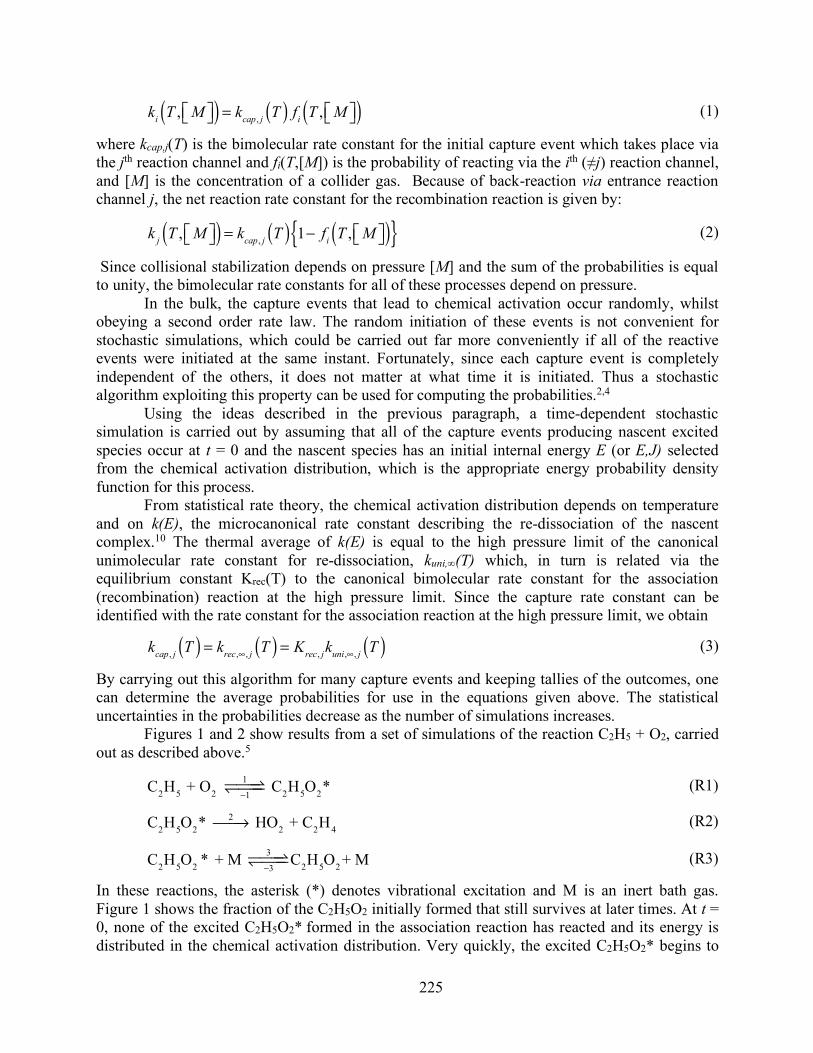
225

(1)

where kcap,j(T) is the bimolecular rate constant for the initial capture event which takes place via the jth reaction channel and fi(T,[M]) is the probability of reacting via the ith (≠j) reaction channel, and [M] is the concentration of a collider gas. Because of back-reaction via entrance reaction channel j, the net reaction rate constant for the recombination reaction is given by:

(2)

Since collisional stabilization depends on pressure [M] and the sum of the probabilities is equal to unity, the bimolecular rate constants for all of these processes depend on pressure.

In the bulk, the capture events that lead to chemical activation occur randomly, whilst obeying a second order rate law. The random initiation of these events is not convenient for stochastic simulations, which could be carried out far more conveniently if all of the reactive events were initiated at the same instant. Fortunately, since each capture event is completely independent of the others, it does not matter at what time it is initiated. Thus a stochastic algorithm exploiting this property can be used for computing the probabilities.2,4

Using the ideas described in the previous paragraph, a time-dependent stochastic simulation is carried out by assuming that all of the capture events producing nascent excited species occur at t = 0 and the nascent species has an initial internal energy E (or E,J) selected from the chemical activation distribution, which is the appropriate energy probability density function for this process.

From statistical rate theory, the chemical activation distribution depends on temperature and on k(E), the microcanonical rate constant describing the re-dissociation of the nascent complex.10 The thermal average of k(E) is equal to the high pressure limit of the canonical unimolecular rate constant for re-dissociation, kuni,∞(T) which, in turn is related via the equilibrium constant Krec(T) to the canonical bimolecular rate constant for the association (recombination) reaction at the high pressure limit. Since the capture rate constant can be identified with the rate constant for the association reaction at the high pressure limit, we obtain

(3)

By carrying out this algorithm for many capture events and keeping tallies of the outcomes, one can determine the average probabilities for use in the equations given above. The statistical uncertainties in the probabilities decrease as the number of simulations increases.

Figures 1 and 2 show results from a set of simulations of the reaction C2H5 + O2, carried out as described above.5

(R1)

(R2)

(R3)

In these reactions, the asterisk (*) denotes vibrational excitation and M is an inert bath gas. Figure 1 shows the fraction of the C2H5O2 initially formed that still survives at later times. At t = 0, none of the excited C2H5O2* formed in the association reaction has reacted and its energy is distributed in the chemical activation distribution. Very quickly, the excited C2H5O2* begins to

ki T , M⎡⎣ ⎤⎦( ) = kcap, j T( ) fi T , M⎡⎣ ⎤⎦( )

k j T , M⎡⎣ ⎤⎦( ) = kcap, j T( ) 1− fi T , M⎡⎣ ⎤⎦( ){ }

kcap, j T( ) = krec,∞, j T( ) = Krec, jkuni,∞, j T( )

C2H5 + O2 1

−1! ⇀!!↽ !!! C2H5O2*

C2H5O2* 2⎯→⎯ HO2 + C2H4

C2H5O2 * + M 3

−3! ⇀!!↽ !!! C2H5O2 + M

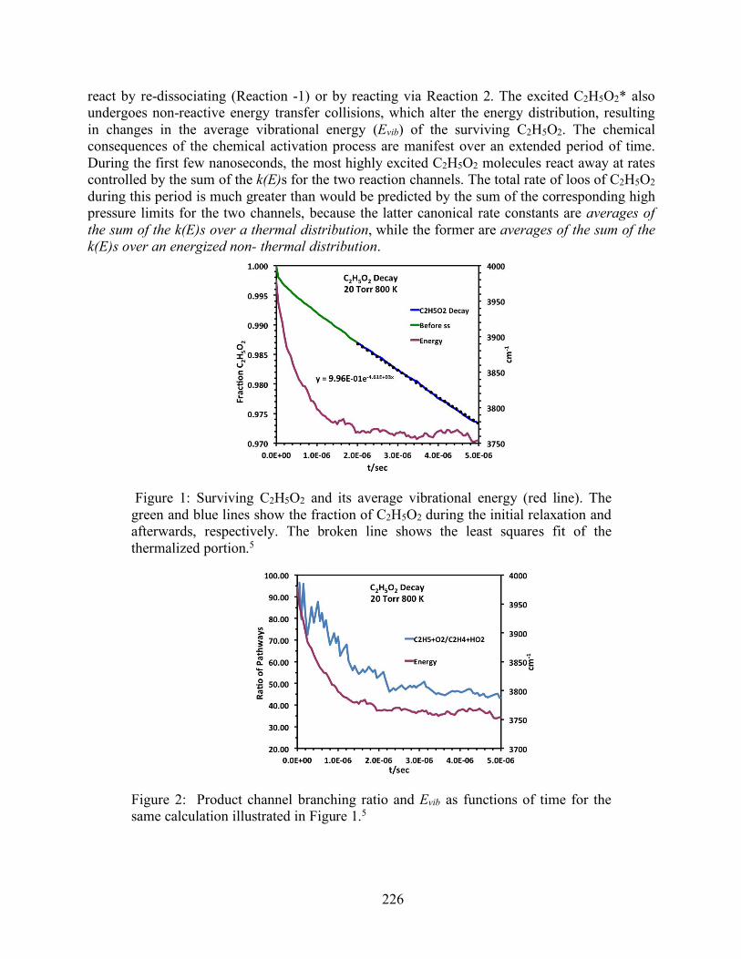
226

react by re-dissociating (Reaction -1) or by reacting via Reaction 2. The excited C2H5O2* also undergoes non-reactive energy transfer collisions, which alter the energy distribution, resulting in changes in the average vibrational energy (Evib) of the surviving C2H5O2. The chemical consequences of the chemical activation process are manifest over an extended period of time. During the first few nanoseconds, the most highly excited C2H5O2 molecules react away at rates controlled by the sum of the k(E)s for the two reaction channels. The total rate of loos of C2H5O2 during this period is much greater than would be predicted by the sum of the corresponding high pressure limits for the two channels, because the latter canonical rate constants are averages of the sum of the k(E)s over a thermal distribution, while the former are averages of the sum of the k(E)s over an energized non- thermal distribution.

Figure 1: Surviving C2H5O2 and its average vibrational energy (red line). The green and blue lines show the fraction of C2H5O2 during the initial relaxation and afterwards, respectively. The broken line shows the least squares fit of the thermalized portion.5

Figure 2: Product channel branching ratio and Evib as functions of time for the same calculation illustrated in Figure 1.5

227

After the first few nanoseconds, the most highly excited C2H5O2* molecules have already reacted away and surviving molecules react away more slowly. During the period up to ~2 µs, the C2H5O2 decay is almost, but not quite, first order, suggesting that the chemical activation event has concluded. A more sensitive diagnostic, Evib for the surviving C2H5O2 molecules, shows that the energy distribution is still evolving and the chemical activation process is still underway up to ~2 µs. Figure 2 shows that the branching ratio between the two dissociation pathways changes by about a factor of two during this period. This change is due to the changes in the energy distribution function that are taking place during this initial energy relaxation period.

From simulations such as these, it is convenient to define the bimolecular chemical activation rate constants in terms of the probabilities evaluated at the end of the initial relaxation period. Subsequent reaction of the thermalized species takes place at a rate controlled by the thermal reaction. Thus a single simulation can be used to obtain both the chemical activation rate constant and the thermal rate constant.

When the time scales of energy relaxation and the subsequent reactions of the thermalized intermediate in a single channel reaction (e.g. C2H5O2) are widely separated, it is easy to identify the end of the initial relaxation as the time when Evib and the reaction flux coefficients become constant.5 For multi-channel reactions, the end of the initial relaxation is less distinct even under favorable circumstances, since isomerization reactions can affect both Evib and the reaction flux coefficients.6,15 Under most conditions, the initial relaxation seldom requires more than a few hundred collisions (when using typical Lennard-Jones and energy transfer parameters).

At the High Pressure Limit The best way to compute the infinite pressure limit rate constants for recombination and unimolecular reaction is to use THERMO, which has the capability to compute canonical transition state theory rate constants (CTST), which uses the standard separable approximation (and can include quantum tunneling through an unsymmetrical Eckart barrier), and semi-classical transition state theory (SCTST), which includes full inter-mode coupling and multidimensional quantum tunneling. You will need to supply vibration/rotational constants and relative energies for the reactant(s) and transition state. Note that krec(T,[M]) and kuni(T,[M]), the recombination and unimolecular rate constants at concentration [M] (which is proportional to pressure) and temperature T, are related according to equilibrium constant:

A + B ⇌ C

This relation ship applies at all values of [M].

In the Pressure Fall-Off To compute fall-off rate constants as a function of pressure, two or three steps are

required. The choice of procedure must account for the fact that both forward and reverse

Keq =

krec T , M⎡⎣ ⎤⎦( )kuni T , M⎡⎣ ⎤⎦( )

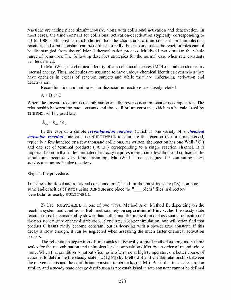
228

reactions are taking place simultaneously, along with collisional activation and deactivation. In most cases, the time constant for collisional activation/deactivation (typically corresponding to 50 to 1000 collisions) is much shorter than the characteristic time constant for unimolecular reaction, and a rate constant can be defined formally, but in some cases the reaction rates cannot be disentangled from the collisional thermalization process. Multiwell can simulate the whole range of behaviors. The following describes strategies for the normal case when rate constants can be defined.

In MultiWell, the chemical identity of each chemical species (MOL) is independent of its internal energy. Thus, molecules are assumed to have unique chemical identities even when they have energies in excess of reaction barriers and while they are undergoing activation and deactivation.

Recombination and unimolecular dissociation reactions are closely related:

A + B ⇌ C Where the forward reaction is recombination and the reverse is unimolecular decomposition. The relationship between the rate constants and the equilibrium constant, which can be calculated by THERMO, will be used later

In the case of a simple recombination reaction (which is one variety of a chemical activation reaction) one can use MULTIWELL to simulate the reaction over a time interval, typically a few hundred or a few thousand collisions. As written, the reaction has one Well ("C") and one set of terminal products ("A+B") corresponding to a single reaction channel. It is important to note that if the unimolecular decay requires more than a few thousand collisions, the simulations become very time-consuming. MultiWell is not designed for computing slow, steady-state unimolecular reactions. Steps in the procedure: 1) Using vibrational and rotational constants for "C" and for the transition state (TS), compute sums and densities of states using DENSUM and place the "____.dens" files in directory DensData for use by MULTIWELL.

2) Use MULTIWELL in one of two ways, Method A or Method B, depending on the reaction system and conditions. Both methods rely on separation of time scales: the steady-state reaction must be considerably slower than collisional thermalization and associated relaxation of the non-steady-state energy distribution. If one runs a longer simulation, one will often find that product C hasn't really become constant, but is decaying with a slower time constant. If this decay is slow enough, it can be neglected when assessing the much faster chemical activation process.

The reliance on separation of time scales is typically a good method as long as the time scales for the recombination and unimolecular decomposition differ by an order of magnitude or more. When that condition is not satisfied, as is often true at high temperatures, a better course of action is to determine the steady-state kuni(T,[M]) by Method B and use the relationship between the rate constants and the equilibrium constant to obtain krec(T,[M]). But if the time scales are too similar, and a steady-state energy distribution is not established, a rate constant cannot be defined

Keq = krec / kuni

229

and it will not be possible to separate the reaction rate from the effects of collisional thermalization. Method A: When the unimolecular decomposition reaction rate is much slower than collisional "thermalizaton", initiate the simulations using the chemical activation energy distribution (key word CHEMACT) for Well "C". Run the simulations for a simulated time duration tmax corresponding to a number of collisions sufficient for thermalizing all of the surviving population of excited "C" (typically 50 to 1000 collisions). Over the course of time, the population of C is affected simultaneously by both collisional deactivation and bond fission back to the initial reactants. Thus the energy of C decreases monotonically until it reaches steady state. At the same time, the yield of C (its "fraction") asymptotically decreases toward a constant value. When the energy of C is low enough, the subsequent very slow steady-state unimolecular bond fission can be neglected. MULTIWELL will report f(C, tmax), the fraction of initial "C" that survives to the end of the simulation (conveniently reported in output file multiwell.sum). If tmax is large enough and bond fission is slow, the numerical value of f(C, tmax) will remain constant even if tmax is increased. The recombination and unimolecular reaction rate constants at that pressure and temperature are given by:

When the reaction is just one of several in a multi-channel reaction system, it is necessary to use the following method. Method B: At high T, when kuni(T,[M]) is fast (i.e. when the time scale for reaction is shorter than the time corresponding to roughly 104 collisions), it is more effective to simulate the unimolecular decomposition reaction. This is accomplished by initiating the reaction of "C" with the thermal energy distribution (key word THERMAL). Multiwell will report f(C,t) the fraction of C that survives to time t in output file multiwell.out. The fraction f(C,t) is proportional to the concentration of species "C" as a function of time. Initially, f(C,t) decays very rapidly as the initial population distribution evolves and converges to the steady-state distribution, which is called the "fall-off" distribution for a simple unimolecular reaction. Once the steady-state distribution has been established, f(C,t) decays exponentially and a plot of ln[f(C,t)] v.s t will give a straight line with slope = −kuni(T,[M]). Thus this method requires plotting the results vs. time and extracting the rate constant. This is easily done using spreadsheets, or data plotting applications.

For chemical activation reactions, the procedures are similar to those for recombination reactions.

A + B ⇌ C → D In a chemical activation reaction, the excited intermediate C initially has enough energy to react and produce product D. The yield ("fraction") of D depends on the competition between collisional deactivation and unimolecular reactions involving the intermediate C. The effective chemical activation rate constant describing the production of D is obtained from the yield of D , which is reported by MULTIWELL as the fraction f(D,t) at the end of the simulation:

krec T , M⎡⎣ ⎤⎦( ) = krec,∞ T( ) ⋅ f C,tmax( )

kA+B→D T , M⎡⎣ ⎤⎦( ) = krec,∞(T ) ⋅ f (D,∞)

230

where krec,∞(T) is the high pressure limit for A + B recombination. With all of these methods, one must bear in mind that the presence of competing

reactions (e.g. reverse reaction and other reaction channels) may strongly influence the steady-state energy distribution, which ultimately controls the reaction rates and derived rate constants. The separation of time scales is often, but not always, sufficient to simplify the analysis. But sometimes it is only possible to determine individual rate constants by analyzing the simulation output just like analyzing experimental kinetics data.

Sometimes, steady state is never established and rate constants cannot be rigorously defined. Even under non-steady-state conditions, however, the Multiwell simulations can be used to accurately model the time-dependent fractions and the final product yields.

231

References

(1) Andraos, J. A Streamlined Approach to Solving Simple and Complex Kinetic Systems

Analytically. J. Chem. Educ. 1999, 76, 1578-1583; DOI: 10.1021/ed076p1578. (2) Barker, J. R. Monte-Carlo Calculations on Unimolecular Reactions, Energy-Transfer, and

IR-Multiphoton Decomposition. Chem. Phys. 1983, 77, 301-318. (3) Barker, J. R. Radiative Recombination in the Electronic Ground State. J. Phys. Chem.

1992, 96, 7361-7367; DOI: 10.1021/j100197a042. (4) Barker, J. R. Multiple-well, multiple-path unimolecular reaction systems. I. MultiWell

computer program suite. Int. J. Chem. Kinet. 2001, 33, 232-245; https://doi.org/10.1002/kin.1017.

(5) Barker, J. R.; Frenklach, M.; Golden, D. M. When Rate Constants Are Not Enough. J. Phys. Chem. A 2015, 119, 7451−7461; DOI: 10.1021/acs.jpca.5b00640

. (6) Barker, J. R.; Frenklach, M.; Golden, D. M. Reply to “Comment on ‘When Rate

Constants Are Not Enough’”. J. Phys. Chem. A 2016, 120, 313−317; DOI: 10.1021/acs.jpca.5b06652.

(7) Bartis, J. T.; Widom, B. Stochastic models of the interconversion of three or more chemical species. J. Chem. Phys. 1974, 60, 3474-3482; doi: 10.1063/1.1681562.

(8) Boyd, S.; Vandenberghe, L. Convex Optimization; Cambridge University Press: Cambridge, UK, 2004.

(9) Duong, M. V.; Nguyen, H. T.; Truong, N.; Le, T. N. M.; Huynh, L. K. Multi-Species Multi-Channel (MSMC): An Ab Initio-based Parallel Thermodynamic and Kinetic Code for Complex Chemical Systems. International Journal of Chemical Kinetics 2015, 47, 564-575; doi: 10.1002/kin.20930.

(10) Forst, W. Unimolecular Reactions. A Concise Introduction; Cambridge University Press: Cambridge, 2003.

(11) Frenklach, M.; Packard, A.; Feeley, R. Optimization of Reaction Models with Solution Mapping. In Modeling of Chemical Reactions; Carr, R. W., Ed.; Elsevier: Amsterdam, 2007; Vol. 42; pp 243–291.

(12) Glowacki, D. R.; Liang, C. H.; Morley, C.; Pilling, M. J.; Robertson, S. H. MESMER: An Open-Source Master Equation Solver for Multi-Energy Well Reactions. J. Phys. Chem. A 2012, 116, 9545-9560; 10.1021/jp3051033.

(13) Lewis, E. S.; Johnson, M. D. The Reactions of p-Phenylene-bis-diazonium Ion with Water. J. Am. Chem. Soc. 1960, 82, 5399–5407; DOI: 10.1021/ja01505a027.


(15) Miller, J. A.; Klippenstein, S. J.; Robertson, S. H.; Pilling, M. J.; Shannon, R.; Zádor, J.; Jasper, A. W.; Goldsmith, C. F.; Burke, M. P. Comment on “When Rate Constants Are Not Enough”. J. Phys. Chem. A 2016, 120, 306−312; DOI: 10.1021/acs.jpca.5b06025.

(16) Mucientes, A. E.; Peña, M. A. d. l. Kinetic Analysis of Parallel-Consecutive First-Order Reactions with a Reversible Step: Concentration–Time Integrals Method. J. Chem. Educ. 2009, 86, 390-392; DOI: 10.1021/ed086p390.

232

C.5 How to tell if the simulated time is long enough

Experiments When simulating actual experiments, the simulated time should match the experiment

times. Bear in mind, however, that Multiwell is not intended for simulating slow steady state reactions. Because it simulates every individual collision, it is most suitable for simulated times corresponding to a few thousand collisions, or less. This is quite sufficient for many kinds of experiments with short timescales.

For longer simulations, it is better to use Multiwell to determine individual rate constants and then use those rate constants in an elementary reaction mechanism, which can be solved using a suitable stiff differential equation code. One such code is KINTECUS, which was designed for chemical kinetics and is free of charge for users at academic institutions (available from www.kintecus.com).

Unimolecular Reactions In general, the initial energy distribution assumed in the simulation must relax to the

steady-state distribution. The relaxation time, which depends on the initial energy distribution, is minimized when the assumed initial energy distribution is most similar to the steady-state distribution. For example, if the pressure is high enough so that the reaction is near the high pressure limit, the relaxation time will be minimal if the initial energy distribution is assumed to be thermal (THERMAL). Generally, the initial transient (when the initial distribution is relaxing to the steady-state distribution) is quite manageable when using an initial energy distribution with average energy close to the reaction critical energy. The final steady state distribution does not depend on the particular choice of the initial distribution, whether it is a delta function (DELTA), thermal distribution (THERMAL), or chemical activation distribution (CHEMACT).

The simulation must be run for a simulated time that is sufficient for steady state to be achieved and for the rate constant to be determined. If the rate constant is to be determined by plotting ln(fraction) vs. time (see Section C.4), then plot initially will be non-linear during the transient period when steady state is being established, and subsequently will become linear with slope equal to the desired rate constant. The simulation must be long enough to enable determination of the slope of the straight line portion.

Chemical Activation or Recombination Reactions When simulating chemical activation or recombination reactions, one should run the

simulations long enough to satisfy two criteria:

a) The average energy of a product molecule (C) is well below any of its reaction thresholds (also remember that the distribution of internal energy extends well above the average)

b) The yield of C becomes independent of time (when time-scale separation is sufficient). It is best to carry out some preliminary calculations (using a smaller number of trials) to determine the time duration (or number of collisions) that will be needed for the excited species

233

to be deactivated sufficiently. At low temperatures, this may require only a few dozen collisions, but at high temperatures it may require several hundred.

234

235

C.6 How to deal with Barrierless Reactions Treating barrier-less reactions with "loose transition states" is more complicated than

reactions that have intrinsic energy barriers. There are several choices of methods. Generally, there is a trade-off between ease of use and predictive accuracy. If the method is not being used to predict rate constants, but is instead being used to fit experimental rate constants, then the simpler methods are usually sufficient. For all of the methods, vibrational and rotational constants are usually obtained from quantum chemistry calculations.

In order, starting with the best (and most difficult) method:

1. Microcanonical variational transition state theory (mVTST): In the MultiWell Software Suite, this method has been implemented in program ktools, which computes canonical (thermal) VTST rate constants (cVTST rate constants) as well as microcanonical sums and densities of states, which are appropritate for master equation simulations. 2. Canonical transition state theory (CTST), which uses molecular constants to compute partition functions: CTST is implemented in thermo, which can be used with molecular constants along a reaction path to find the canonical variational transition state and a corresponding cVTST rate constant. The molecular data required for this calculation are exactly the same as those used by ktools, but the ktools calculations are preferred, because they are significantly more accurate.

3. Hindered Gorin model: see Index of this User Manual. 4. Inverse Laplace transform method: a built-in option in MULTIWELL (key word ILT). This method is often investigated first, because it is the easiest and least expensive, but alos the least accurate. Methods #1 to #4 can be employed relatively easily in Multiwell. Method #1 is preferred. Typically, #3 and #4 are used empirically by fitting a known (or estimated) thermal rate constant at a given temperature. Several applications of methods #2, #3, and #4 are described in recent articles.1-4

References

(1) Ali, M. A.; Barker, J. R. Comparison of Three Isoelectronic Multiple-Well Reaction

Systems: OH + CH2O, OH + CH2CH2, and OH + CH2NH. J. Phys. Chem. A 2015, 119, 7578−7592; DOI: 10.1021/acs.jpca.5b00910.

(2) Ali, M. A.; Sonk, J. A.; Barker, J. R. Predicted Chemical Activation Rate Constants for HO2 + CH2NH: The Dominant Role of a Hydrogen-Bonded Pre-reactive Complex. J. Phys. Chem. A 2016, 120, 7060−7070; DOI: 10.1021/acs.jpca.6b06531.

(3) Golden, D. M.; Barker, J. R. Pressure- and Temperature-Dependent Combustion Reactions. Combust. Flame 2011, 158, 602–617.

(4) Yang, L.; Sonk, J. A.; Barker, J. R. HO + OClO Reaction System: Featuring a Barrierless Entrance Channel with Two Transition States. J. Phys. Chem. A 2015, 119, 5723–5731; DOI: 10.1021/acs.jpca.5b03487.

236

C.7 Some Questions and Answers (Most of the answers were written by JRB; Some questions and answers are rather old!)

1. QUESTION: Every molecule has a 2 dimensional external inactive rotor and an external active rotor (the K-rotor). I can see where the external inactive rotor goes but I'm not sure about the external active rotor.

ANSWER: The parameters "MolMom" on line #8 and "RR" on line #15 of the data file are moments of inertia for the 2-dimensional external (inactive) rotors for the reactant and the transitions state, respectively. The external active rotor is included with the other degrees of freedom in the density and sum of states calculation. Therefore it is included in the data file for SumDen. For example, O3 (ozone) has 3 vibrations and 3 rotations. The SumDen data file should include 4 degrees of freedom: 3 vibrations + 1 rotor (the active external rotation, which I usually label the "K-rotor"). The moment of inertia for the remaining 2-D external (inactive) rotor appears on line #15.

2. QUESTION: If there is an internal active rotor, do I remove the vibration associated with it from the Densum input?

ANSWER: An internal degree of freedom is either a rotor, or a vibration...not both. Thus, if you have a vibrational assignment (from Gaussian, say), you may wish to replace a low frequency vibrational mode with a free rotor mode. Then you remove the vibration and insert the rotor in its place, so that the number of internal degrees of freedom is preserved.

3. QUESTION: In all your examples you use an energy spacing of 10 cm-1 and when I use 1 cm-1 the code freezes. Do you recommend using 1 cm-1 and if so should I increase the size of the array, which is currently 14000?

ANSWER: We usually recommend 10 cm-1, because we have found that for most systems it gives excellent numerical convergence at room temperature and above, and because few thermochemical values are known to better accuracy. In previous work, 25 cm-1 spacing also worked very well. If you want to use a smaller grain size, then the arrays should be increased in size. In principle, one should always test to make sure that the grain size is small enough so that it does not affect the results significantly.

4. QUESTION: In using DenSum, when should one use quantum state counting for rotors ("qro") and when should one use classical state densities ("rot")?

ANSWER: As a rough rule of thumb, if the rotational constant is greater than B = 1 cm-1, use "qro"; if it is less than 0.1 cm-1, use "rot"; in between, you can try it both ways and then decide if the difference will affect your calculations. If you use "qro" for a case where the rotational constant is extremely small, there may be computational problems... this limit has not been tested thoroughly … and it would be better to use "rot".

237

5. QUESTION: What will happen if the density of states function is not a smooth, continuous function at energies corresponding to the upper half of the double array?

ANSWER: Subroutine COLSTEP assumes that the density of states is smooth in the upper portion of the double array. In general, you should plot the density of states vs. E to confirm that the energy dividing the two portions of the double array is high enough so that the density of states does not fluctuate more than, say, 5%. If the fluctuations are larger, they will cause problems in selecting the step sizes, resulting in anomalously large probabilities of large activating steps.

6. QUESTION: Why does my compiler have trouble reading the example data files that contain names (CHARACTER CONSTANTS)?

ANSWER: If your compiler does not accept the CHARACTER CONSTANTS in the example data files, enclose the CHARACTER CONSTANTS in apostrophes (') and try again. "Free format" (list directed input) is used by the MultiWell suite. Different compilers may choose to use different delimiters to separate the input fields in free format. Most compilers use commas and spaces, but some also will recognize tabs, returns, linefeeds, and other characters. Most compilers will recognize CHARACTER CONSTANTS (e.g. file names and chemical species names) when they are contained in apostrophes (e.g. 'xyz'). Other compilers will also accept quotes (e.g. "xyz"), or text without any special enclosing delimiters (e.g. xyz).

7. QUESTION: How can the 2-D hindered rotations in loose transition states be handled using DenSum?

ANSWER: There are at least three different ways 2D-hindered rotors for loose transition states can be handled by DenSum. The first is by using the restricted Gorin prescription of Smith and Golden6 (see Benson's discussion1 of the Hindered Gorin Model), which is based on a modified version of the Gorin Model.2 The second is to replace the restricted rotor formulation with one based on particle-in-a-box. The third is to use two 1-D hindered rotors (implemented in DenSum) instead of one 2-D hindered rotor (2-D hindered rotors are not implemented in DenSum).

Smith and Golden6 use a "hindrance parameter" to modify the moment of inertia of a 2-D free rotor: the Hindered Gorin Model. They find the value of the hindrance empirically by varying it until they achieve a fit with experimental rate constant data. In my opinion, a potential drawback of the Smith and Golden approach is that the rotor model has no zero point energy, and restricting the range of rotational motion results in a model that is more like a particle-in-a-box, which has a finite zero point energy. It is for this reason that I added the particle-in-a-box degree of freedom type to DenSum. The zero point energy is important because of the role it plays in isotopic reactions. To use particle-in-a-box energy levels (instead of free rotor levels), one can empirically vary the "frequency" parameter until agreement with experiment is achieved, just as done by Smith and Golden.

The third alternative is to use two 1-D hindered rotors for each 2-D internal rotation. Here, the moment of inertia can be used directly in DenSum and the hindrance potential is then varied until agreement with the rate constant data is achieved. I've done a few brief tests of this

238

approach and it seems to work well. The use of an actual hindered rotor is attractive to me, because it seems more physically realistic (one of these days we'll investigate this using quantum chemical calculations). The drawback is that state degeneracies may not be calculated correctly.

I don't know if there is a significant difference among rate constants calculated using the methods described above. Each of the methods is probably quite adequate in fitting almost any experimental data (a detailed comparison of the methods would be quite interesting). However, making predictions for temperatures where no experimental data are available requires formulation of an ad hoc model for hindrance as a function of temperature. Jordan, Smith, and Gilbert3 have formulated such a model (based on free rotors) and have tested it for a few cases; it is possible that their method could be used with Densum. The Marcus and Wardlaw approach7,8 is more predictive, but only if an accurate multi-dimensional potential energy surface is available. Miller and Klippenstein5 have used VariFlex software,4 which implements an extended version of the Marcus-Wardlaw approach.

8. QUESTION: Why is the output "noisy" and what is the meaning of the columns labeled "+/-error"?

ANSWER: Multiwell works by carrying out stochastic trials, each of which is a random walk governed by the physics of the reaction system. In each trial, one or more wells may be "visited' during the random walk and the random walker will be found in a well or reaction product at the end of the trial. Multiwell carries out stochastic trials one at a time and sums up the results. But it is convenient to discussed the summed result as if a whole "swarm" of random walkers was released at the same time... an equivalent procedure. During a set f trials, each of the time steps records a "snapshot" of the number of walkers in each well or product set at the instant of the time step. The fractions are based on these snapshots.

For a set of, say, N=100 stochastic trials, there are 100 random walkers. If only one random walker out of the whole set is in a well at the time of a snapshot, then the corresponding fraction is 0.01. If 37 are in the well, then the fraction is 0.37. The smallest possible non-zero fraction (greater than zero) is equal to 1/N. Furthermore, for a finite number of stochastic trials, a statistical error is associated with each fraction. The estimated statistical error (specifically, 1 standard deviation) is reported by multiwell in the columns labeled "+/-Error". As the number of stochastic trials is increased, the smallest non-zero fraction decreases and the statistical error decreases. Thus changing the number of trials will produce small changes in the fractions... changes that should be consistent with the actual statistical fluctuations. (The theory behind the estimated statistical errors is presented in Appendix A.3.2 of the User Manual.)

When carrying out longer trials, the last "snapshot" occurs at a later time and the fraction recorded by the final snapshot (reported in output file multiwell.sum) may vary with time. Even if equilibrium has been achieved and no further time variation is expected, the stochastic "noise" (i.e. statistical errors) associated with the finite number of stochastic trials may be observed, but it should be consistent with the estimated statistical errors.

It is not possible to completely eliminate the stochastic noise for a finite number of trials. You should decide what level of noise is tolerable... i.e. what statistical precision is needed... and set the number of trials accordingly. A very large number (millions) of stochastic trials may be needed to obtain high precision results for a reaction product that is produced with a very small fractional yield. The required computer time is proportional both to the number of trials and to

239

the length of simulated time (see Appendix A.3.2). As a result, certain simulations are simply not feasible, or they may be feasible if creative alternative approaches are devised.

References

(1) Benson, S. W. Thermochemical Kinetics, 2nd ed.; Wiley: New York, 1976. (2) Gorin, E. Photolysis of acetaldehyde in the presence of iodine. Acta Physicochim., URSS

1938, 9, 681. (3) Jordan, M. J. T.; Smith, S. C.; Gilbert, R. G. Variational transition state theory: a simple

model for dissociation and recombination reactions of small species. Journal of Physical Chemistry 1991, 95, 8685-8694.

(4) Klippenstein, S. J.; Wagner, A. F.; Robertson, S. H.; Dunbar, R.; Wardlaw, D. M. VariFlex Software; 1.0 ed.; Argonne National Laboratory, 1999.

(5) Miller, J. A.; Klippenstein, S. J. Theoretical Considerations in the NH2+ NO Reaction. J. Phys. Chem. A 2000, 104, 2061-2069.

(6) Smith, G. P.; Golden, D. M. Application of RRKM Theory to Reactions OH+NO2+N2 = HONO2+N2 (1) and ClO+NO2+N2 = ClONO2+N2 (2) - Modified Gorin Model Transition-State. IJCK 1978, 10, 489.

(7) Wardlaw, D. M.; Marcus, R. A. Unimolecular Reaction-Rate Theory for Transition-States of Any Looseness. 3. Application to Methyl Radical Recombination. Journal of Physical Chemistry 1986, 90, 5383-5393.

(8) Wardlaw, D. W.; Marcus, R. A. RRKM reaction rate theory for transition states of any looseness. J. Chem. Phys. 1984, 110, 230-234.

240

Index

<name>.dens, 95 <name>.qcrp, 95 2 dimensional rotor, 236 2-D adiabatic rotor, 154 2-D hindered rotations, 237 2-dimensional external rotation, 31 3-D relative translation, 168 Accuracy

Thermo, 67 active energy, 23, 194 active rotor, 236 adensum, 83 Adiabatic Channel Model, 155 adiabatic rotor, 192 A-factor, 33 angular momentum, 154 ANH, 188 Anharmonic oscillator, 48 anharmonicity coefficients, 94, 189 anharmonicity constants, 190 ansum, 83 asymmetric top, 193 atom type, 64 atom types, 202 atomic mass, 202 ATYPE, 64 average vibrational energy, 226 averaged results, 151 barrier-less reactions, 235 batch option, 60 bdens, 11, 12, 48, 83

program, 66 bdens, 211 BEST, 211 BETTER, 211 Beyer-Swinehart algorithm, 58 Biexponential Model, 38 bimolecular, 165 bimolecular microcanonical transition state theory,

36 bimolecular reaction, 36 bimolecular reactions

competing with unimolecular, 165 BIMOLRXN, 36 BIMOLRXN option, 165 BJ, 50 BK, 50 canonical bimolecular rate constant, 166 canonical rate constant

trial, 115 canonical transition state theory, 6, 160

Canonical transition state theory, 235 Canonical Transition State Theory, 67 capture rate constant, 225 CENT1, 34, 215 CENT2, 34, 160, 215 centrifugal corrections, 137, 160, 194 CENTX, 34, 215 CFOUR, 208, 212 checkpoint file, 95 CHEMACT, 37 chemical activation, 224 Chemical activation, 37 Chemical Activation, 180 chiral stereoisomer, 197 COLL, 37 collision frequency, 139, 171, 174 collision integral, 32, 171, 173 collision models, 32, 37 collision step-size distribution, 138, 171 collision-induced IVR, 35, 160 competition between unimolecular and bimolecular

reactions, 167 compiler options, 24 computation time, 223 computer time, 151, 238 convergence tests, 147 Conversion Factors, 188 convolution, 168 cpu time, 224 critical energy, 23, 33, 154, 212 CRP, 94, 210, 211 CTST, 235 cumulative reaction probabilities, 7 cumulative reaction probability, 34, 94 cVTST, 235 data files, 78 defaults, 24 definitions, 22 degeneracies, 192 degrees of freedom, 69 DELTA, 37 DensData, 37 DensData, 41 densities of states, 41, 146 Density Functional Theory, 158 density of states, 237 densum, 9, 48 DenSum, 136, 236 densum.batch, 60

Batch file format, 60 densum.lev, 58 densum.out, 58

241

detailed balance, 139, 172 directory DensData, 25, 37

dissociation energy, 190 dividing surface, 115 doloops, 83 DO-loops, 211 double array, 121 Double array, 29, 146 double-well potential, 198 Eckart barrier, 6, 33, 73, 161 Egrain1, 29, 44, 59 Einit, 37 Elements, 202 Emax2, 29, 44, 59 energy grain, 146 energy relaxation, 221 Energy schematic, 23, 136 energy transfer, 32 energy transfer parameter, 220 energy units, 30 energy units for THERMO, 67 enthalpy for formation, 67 Enthalpy function

[H(T)-H(0)], 67 enthalpy of formation, 31 entropy, 67 equilibrium constant, 66 Equilibrium constant, 67 Eunits, 30 exact counts, 136 Example multiwell Models, 15 exponential Model, 38 Exponential model, 37 exponential-down model, 220 EXTERNAL, 37 external file, 34 external symmetry number, 50 EXTRA, 211 FAIR, 211 fall-off, 229 FAST, 33 filename

user-defined, 25, 63, 72 FileName, 25, 26, 28 fit, 68 Fitting Experimental Rate Constants, 68 Flexible Transition State Theory, 155 flux coefficient, 26, 184 FUN, 48, 58, 75, 189 fundamental frequency, 48 gauche structures, 197 gauss2multi, 12, 78 GAUSSIAN, 212 Gaussian 03, 78 Gaussian 98, 78

getting started, 5 Gillespie Exact Stochastic algorithm, 22 Gillespie's Exact Stochastic Method, 150 GOOD, 211 gor, 68 Gorin model, 157 Gorin Model, 237 grain size, 236 HAR, 58, 59, 75, 87, 96 harmonic frequency, 48, 188 Harmonic oscillator, 48 Heat Capacity, 67 high pressure limit, 159 high pressure rate constant, 160 Hindered Gorin model, 235 Hindered Gorin Model, 68, 155, 157, 237 hindered internal rotation, 106, 136, 196 Hindered internal rotation

General, 51, 54, 196 Optical isomers, 197 symmetrical, 51

hindered rotor symmetrical, 53

hindrance parameter, 68, 237 Hmol, 31 HMol, 31 hybrid master equation, 145 hydrogen peroxide, 197 IDUM, 29 ILT, 34 imaginary frequency, 34, 94, 162 imax1, 29, 44 Imax1, 59 IMol, 31 inelastic collision frequency, 172, 174 inelastic collisions, 172 initial conditions, 179 initial energy relaxation, 221 initial relaxation, 227 initial well, 37 INPUT ERRORS, 44 internal rotation, 136

optical isomers, 197 unsymmetrical, 196

internal rotor symmetry, 195 internal rotors, 51 Internal rotors, 195 intrinsic upper limit, 124 Inverse Laplace Transform (ILT) Method, 156 Inverse Laplace transform method, 235 Isize, 29, 44, 59 isomerization, 145 IVR, 137, 160 IVR threshold energy, 35 IVR transmission coefficient, 34, 160 J-summed, 11

242

densities of states, 120 sums of states, 120

J-summing, 120, 121 K quantum number restrictions, 50 k(E), 183 KEYWORD, 33, 37 Klaus Luther's empirical function, 40 K-rotor, 53, 135, 136, 154, 193, 236 ktools, 11, 48, 113, 235 ktools.dat, 124 lamm, 12, 106, 137 Laplace transform, 168 large amplitude motions, 106 Lennard-Jones parameters, 32, 171, 220

Table, 201 linear master equation, 151 LOGT, 37 loose transition state, 155, 235 loose transition states, 237 low pressure limit, 159 master equation, 135

J-resolved, 8, 134 steady-state, 8, 134

maximum number of collisions, 37 microcanonical, 165 microcanonical bimolecular rate constant, 165 microcanonical rate constant, 94 microcanonical transition state theory, 165 Miller, W. H., 207 Miller, W. H., 94 Miller, W. H., 208 mirror image, 197 molecular constants

sources, 76 Molele, 31 Molinit, 37 MolMom, 31 MolName, 31 Molopt, 31 Molsym, 31 moment of inertia, 31 Moment of Inertia, 188 moments of inertia, 63 mominert, 10, 12 MORSE, 69 Morse oscillator, 48, 188 Morse Oscillator, 69 Morse oscillator anharmonicity, 48 Morse Potential, 158 multinomial distribution, 152 multiple-transition state model, 117 multiple-well systems, 145 multiwell, 13 MultiWell, 22

Data files, external, 41, 43

Examples, 157, 179 Input File, 5, 182 Input file format, 29, 58 Output files, 58, 183 Symmetry Examples, 199

MultiWell input options, 28 multiwell.array, 26, 184 multiwell.dist, 26, 184 multiwell.flux, 27, 184 multiwell.out, 26, 183 multiwell.rate, 26, 184 multiwell.sum, 26 mVTST, 235 NOCENT, 34, 160, 215 noise, 222 non-RRKM, 160 non-separable degrees of freedom, 94 non-separable vibrations, 189 NOREV, 33 normalization, 172, 173 normalization problems, 173 normalization, finite difference algorithm, 174 NOTUN, 33 Np, 30 NProds, 31 number of trials, 37 numerical convergence, 220, 236 NWells, 31 oblate symmetric top, 194 oblate top, 154 obs, 48 OLDET, 32 optical isomer, 197 optical isomers, 31, 33 Optical isomers

Hindered internal rotation, 197 output files, 26 paradensum, 7, 11, 12, 48, 89, 90

program, 66 Particle in a Box, 50 particle-in-a-box, 53, 237 partition function, 94, 168 perturbation theory expansion, 189 Photo-Activation, 180 precision, 152 pressure units, 30 Product set, 31 Product sets, 31 Product sets, defined, 22 Program Execution, 25 prolate symmetric top, 194 prolate top, 154 pseudo-diatomic model, 154 pseudo-first-order, 165 Punits, 30 qro, 236

243

quantum mechanical tunneling, 212 Quantum mechanical tunneling, 161 quasi-bound states, 191 quasicontinuum, 137 quasi-symmetric top approximation, 193 Questions and Answers, 236 radiationless transitions, 40 random number generator, 152 random walkers, 238 rate constant

canonical, 208 chemical activation, 230 microcanonical, 208 unimolecular, 228

Reactant Sets, 22 reaction flux coefficient, 26, 184 reaction flux coefficients, 227 reactive flux, 142, 184 recombination, 224 recombination reaction, 69 Recombination Reactions, 180 re-crossing, 115 reduced moment of inertia, 63, 107 relative translation, 52 restricted Gorin model, 157 REV, 33 RKE, 34 rot, 236 rotation, 53, 135

quantized, 53 Rotation, 49 rotational, 30 Rotational Constant, 188 rotational constants, 30 rotational degrees of freedom, 69 rotations of a linear molecule, 49 rotations of a non-linear molecule, 49 rotations of a spherical top molecule, 49, 50 Rotatunits, 30 RRKM theory, 153 Schrödinger equation, 106 sctst

program, 66 sctst, 12, 13, 48 SCTST, 66, 70, 94, 95, 193, 207, 211 SCTST, limitations, 209 sctst.out, 94, 95 selection of step sizes, 174 semi-classical transition state theory, 70, 94, 207 Semi-Classical Transition State Theory (SCTST), 7 Semi-empirical Canonical Variational Transition

State Theory, 158 semi-microcanonical bimolecular rate constant, 166 semi-microcanonical pseudo-first order rate constant,

167 separable rotors approximation, 194

separable-rotors approximation, 141, 193 separation of time scales, 228 shock-tube simulations, 30 simulated time, 232 SLOW, 33, 34 Slow IVR, 160 sMORSE, 69 source code, 24 specific rate constants, 41, 146 spherical top, 49, 50, 192, 193

separable rotors approximation, 193 standard state, 66 statistical errors, 238 statistical fluctuations, 238 steady-state distribution, 229 step-size distribution, 175 Stiff Morse Oscillator, 69 Stochastic Method, 150 stochastic noise, 238 stochastic sampling noise, 222 stochastic trials, 238 SUM, 34 sums and densities of states, 210 sums of states, 41, 146 symmetric top, 49, 53, 192

separable rotors approximation, 193 symmetric tops

almost symmetric, 155, 193 symmetry

internal rotation, 195 potential energy, 195

symmetry number, 31, 33 hindered internal rotation, 54

symmetry numbers, 154 Symmetry Numbers, external, 195 symmetry numbers, internal rotors, 195 Temp, 30 terminology, 22 THERMAL, 37 Thermal Activation, 179 thermo

program, 66 thermo, 9, 12, 48 THERMO, 158 thermodynamics database, 76 threshold energy, 154 tight transition state, 154 time, 37 TIME, 37 time step, 151 top, 53 torsion, 136 torsion rotational constant function, 137 torsions, 106 total collision rate constant, 32 total collision frequency, 35

244

total collision rate constant, 161, 171 transition state, 73

loose, 155 tight, 154

Transition state parameter entry, 33 transition state theory, 66, 94, 207 transition states, 145 Transition states, 22 translation, 55 Translation, 52 translational states, 169 translational temperature, 30 trial transition states, 113 trn, 55 TS computer code, 134 tun, 213 TUN, 33, 34 tunneling, 33, 73, 94, 161, 208 tunneling corrections, 6 tunneling probability, 161 Tvib, 30 Uncertainties, 152 unified rate constant, 117 Unimolecular Reactions, 153 unsymmetrical hindered internal rotation, 51 utilities, 78 utilities for creating data files, 78 variational transition state theory, 235

canonical, 113, 114 J-resolved, 113, 117 microcanonical, 113, 117

Variational Transition State Theory, 155 VariFlex software, 238 VARSHNI, 69 Varshni Oscillator, 69 Viblo, 41 vibration, 53 vibrational

anharmonicity, 188 vibrational anharmonicity, 70, 207 vibrational energy, 188

perturbation theory expansion, 189 vibrational perturbation theory, 212 vibrational temperature, 30 vibrations

non-separable, 189 separable, 188

vimag(Mol,i), 34 VPT2, 97, 212 VPT4 correction, 97 VPT4A, 97 VPT4B, 97 VPTx, 97 Wang-Landau algorithm, 94 Warnings, 44 wells, 145 Wells, 31 Wells, defined, 22 Whitten-Rabinovitch approximation, 58 Xij anharmonicity coefficient matrix, 188

Documents

MultiWell User Manual-2020 - University of Michigan