- Munich Personal RePEc Archive - Is there any relationship between … · 2019-09-26 · Munich Personal RePEc Archive Is there any relationship between Economic Growth and Human

Munich Personal RePEc Archive

Is there any relationship between

Economic Growth and Human

Development? Evidence from Indian

States

Mukherjee, Sacchidananda and Chakraborty, Debashis

National Institute of Public Finance and Policy (NIPFP), NewDelhi, Indian Institute of Foreign Trade (IIFT), New Delhi

31 May 2010

Online at https://mpra.ub.uni-muenchen.de/22997/

MPRA Paper No. 22997, posted 01 Jun 2010 17:30 UTC

Is there any relationship between Economic Growth and Human

Development? Evidence from Indian States#

Sacchidananda Mukherjee1*

and Debashis Chakraborty2

* Corresponding author

1 Assistant Professor, National Institute of Public Finance and Policy (NIPFP), 18/2, Satsang Vihar Marg,

Special Institutional Area, New Delhi – 110 067, INDIA. Telephone: +91 11 2656 9780; +91 11 2696

3421; Mobile: +91 9868421239; Facsimile: +91 11 2685 2548. E-mail: [email protected]

2 Assistant Professor, Indian Institute of Foreign Trade (IIFT), IIFT Bhawan, B-21, Qutab Institutional

Area, New Delhi 110016, India. Fax: +91-11-2685-3956. E-mail: [email protected]

Abstract

The paper attempts to analyse the relationship between economic growth and human

development for 28 major Indian States during four time periods ranging over last two decades:

1983, 1993, 1999-00 and 2004-05. To construct Human Development Index for Indian States, we

consider the National Human Development Report 2001 Methodology. The objective of this

exercise to understand at what degree and extent the per capita income (as an indicator of

economic growth) has influenced the human development across Indian States. To understand

the rural – urban disparity in the achievement of human development, the Human Development

Index is constructed for rural and urban areas separately for each of the States. The result shows

that that per capita income is not translating into human well being. This perhaps in another

way might signify the rising influence of other variables in determination of the HD achievements

of a state. The result shows the need for further investigation to determine the underlying

factors (other than per capita income) which influence HD achievements of a State.

Keywords: Economic Growth, Human Development, Human Development Index

Methodology, Economic Liberalisation, Indian States.

JEL Classification Codes: O47, O15, E21, H75, C01,

��

1

Is there any relationship between Economic Growth and Human

Development? Evidence from Indian States

Sacchidananda Mukherjee Debashis Chakraborty

Assistant Professor Assistant Professor

National Institute of Public Finance and Policy Indian Institute of Foreign Trade

18/2, Satsang Vihar Marg, Special Institutional Area B-21, Qutab Institutional Area

New Delhi – 110 067, India. New Delhi - 110016, India

Phone: +91 11 2656 9780; +91 11 2696 3421 Phone: +91 11 2696 5051

Mobile: +91 9868421239; Fax: +91 11 2685 2548 Fax: +91-11-2685-3956

E-mail: [email protected] E-mail: [email protected]

1. Introduction

The economic reform process initiated since 1991 has played a major role in

determining India’s overall economic growth path. Among the major changes

undertaken during this period, shift in emphasis on export-oriented economic

philosophy, encouragement to FDI inflow, unshackling of industrial licensing, ongoing

tariff reforms (unilaterally as well as part of WTO obligation) need to be mentioned. The

collective influence of these measures has ensured a steady growth path for the country

over the last decade.

The enhanced economic growth (EG), thus generated, is also likely to create

important repercussion effects in the economy, which would further propel the growth

trajectory in the long run. For instance, the rising income level would be instrumental in

expanding the capacity of the government to raise the general level of human

development (HD) in the current period (through provision of health and educational

achievements), which in turn would influence the future EG potential positively.

Over the last decade, India has initiated a number of policy measures for

augmenting HD achievements. For instance, the Sarva Shiksha Abhiyan (SSA) started for

2

universalising elementary education among children aged 6-14 across the states has

been a commendable initiative. Similarly, on the health front the goals of National Rural

Health Mission (NRHM, 2005-12) includes: reduction in Infant Mortality Rate (IMR) and

Maternal Mortality Ratio (MMR), universal access to public health services such as

women’s health, child health, water, sanitation & hygiene, immunisation, and nutrition,

prevention and control of communicable and non-communicable diseases, including

locally endemic diseases etc. The introduction of National Rural Employment Guarantee

Act (NREGA) in rural areas and initiation of provisions like Right to Education Act and

Food Security Act in the Parliament are geared for empowering the people with right to

employment, food and education. All these measures are expected to enable India to

move closer to fulfillment of the related Millennium Development Goals by the

stipulated deadline, 2015. On the economic front, the growing size of the healthy and

educated population in the working age group, resulting from the aforesaid policy

measures, is expected to enable the country to reap the benefits of Demographic

Dividend more vigourously.

In this background, on the basis of a secondary data analysis, the current paper

attempts to analyse the relationship between EG and HD for 28 major Indian States

during four time periods ranging over last two decades: 1983, 1993, 1999-00 and 2004-

05. The objective of this exercise to understand at what degree and extent the per

capita income (as an indicator of economic growth) has influenced the human

development across Indian States. To understand the rural – urban disparity in the

achievement of human development, the Human Development Index is constructed for

rural and urban areas separately for each of the States. While 1983 marks the pre-

liberalisation era, 1993 captures the scenario shortly after initiation of the reform

exercises. Though the reform process was almost a decade old during 1999-00, the EG in

the preceding period was influenced by several external and internal events (e.g.

Southeast Asian Crisis during 1997-98, three General Elections over 1996-99 etc.). On

the other hand, 2004-05 marked a period of relative stability.

3

The paper is organised as follows. A brief literature survey on the relationship

between EG and HD is followed by a discussion on the methodology adopted in this

paper, the empirical results and the policy observations respectively.

2. Economic Growth and Human Development

The existing literature suggests the presence of a two-way relationship between

EG and HD, implying that nations / states may enter either into a virtuous cycle of high

growth and large HD gains, or a vicious cycle of low growth and low HD improvement

(Ranis, 2004; 2000). Higher initial level of HD may also lead to positive effects on

institutional quality and indirectly on EG (Costantini and Salvatore, 2008). It has been

observed that India displays a two-way causality between EG and HD, indicating

possibilities of vicious cycles (Ghosh, 2006).

The existing governance mechanism or institutions in a country can play a key

role in strengthening the EG-HD relationship. Amin (undated) noted that institutions

contribute significantly in EG by expanding the capabilities and by creating an conducive

environment, which ensures proper functioning of the socio-politico-economic life of

societies and economies. Similarly Joshi (2007) concludes that good governance explains

more of HD outcomes (in education, health and longevity) than EG, per capita

investment or per capita income for Indian states during 1980s to the early 2000s. The

study also noted that though there exist positive relationships between HD and EG, they

may not be automatic in either direction.

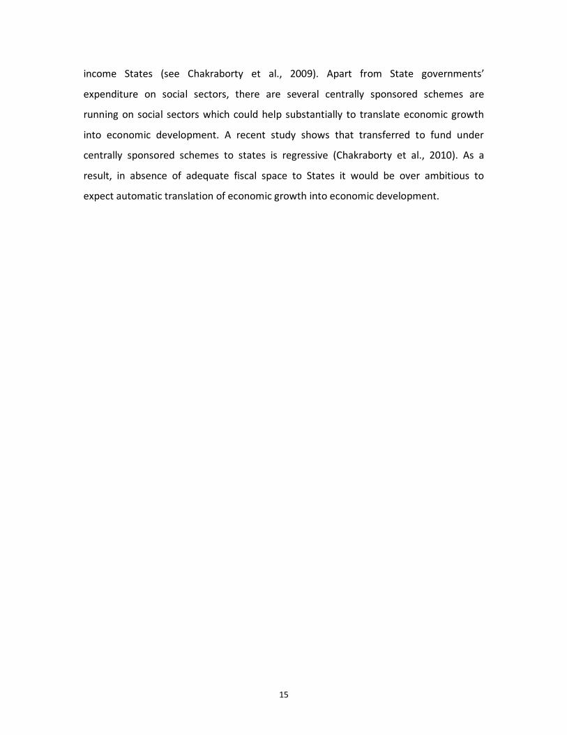
The relationship between Per Capita GDP (in PPP USD) and HDI score (obtained

from UNDP 2009) across countries is presented in Figure 1. The figure shows that, from

cross-country perspective, as per capita income increases the HDI score increases upto a

level and then reaches a plateau. The result indicates that in a multi-country framework,

4

per capita income is necessarily an ingredient for achieving a higher level of human

wellbeing. The cross-country analysis of Mukherjee and Chakraborty (2010) noted that

HD is positively and linearly related to both democracy and income level, indicating that

the countries characterised by higher levels of income and better democratic set up are

likely to witness higher HD achievements.1

An extensive analysis of global HD situation as well as country rankings can be

obtained from the UNDP annual publication of Human Development Report (HDR), from

where India’s achievements on HR front can be ascertained. While India remained in the

low HD category throughout nineties, in 2002 it graduated to medium HD category. In

2005 it secured a composite HDI score of 0.619, as compared to the corresponding

figure of 0.439 in 1990. India’s global HDI rank has also changed from 132 in 1999 to 134

in 2007, while the number of countries covered also increased during this period.

Recently in association with UNDP, the Government of India has started analysing the

State-wise HD status. The National Human Development Report 2001 (Government of

India, 2002), brought out by the Planning Commission, is worth mentioning in this

regard. While the report ranked Kerala, Punjab and Tamil Nadu as the toppers; Bihar,

Madhya Pradesh and Uttar Pradesh were at the other extreme in HD scale. The

alternate index developed by Guha and Chakraborty (2003), in line with Nagar and Basu

(2001), however showed that inclusion of other socio-economic variables changes the

State rankings to some extent.

3 Methodology and Data

3.1 Human Development Index (HDI)

Following the principle of the NHDR 2001 methodology, for calculation of the

Human Development Index (HDI) for Indian States, the current paper consider three

1 The regression results on the relationship between HD and corruption confirms presence of a non-

linearity and suggests that with decline in corruption, HD level rises, but declines marginally for a few

countries characterised by a less corrupt regime (Mukherjee and Chakraborty, 2010).

5

variables, namely - per capita consumption expenditure; composite index of educational

attainment and health attainment respectively. With this formulation, following the HDI

method, the HDI score for the jth

State is given by the average of the normalised values

of the three indicators, namely - inflation and inequality adjusted per capita

consumption expenditure (1

X ); composite indicator on educational attainment (2

X )

and composite indicator on health attainment (3

X ). The normalisation is done by

dividing the difference between any variable ( ijX ) within these categories and the

minimum value of i

X to the difference between the maximum and the minimum value

ofi

X .

Although UNDP considers Real GDP Per Capita in PPP USD for generating the

HDI, the NHDR 2001 has preferred inflation and inequality adjusted average monthly

per capita consumption expenditure (MPCE) of a State over that for the analysis. Here

the monthly per capita consumption expenditure data, obtained from National Sample

Survey Organisation (NSSO)’s quinquennial surveys (38th

Round: 1983, 50th

Round: 1993-

94, 55th

Round: 1999-2000 and 61st

Round: 2004-05), first adjusted for inequality using

State-wise Gini Ratios (also provided in the quinquennial rounds), and further adjusted

for inflation to bring them to 1983 prices by using deflators derived from State specific

poverty line (Government of India, 2002).

For average MPCE it is not only the level of expenditure for a State that is

important to assess the economic attainment, but also the distribution of average MPCE

across population of the State (which is captured through Gini Ratio). A State with high

average MPCE with lower Gini Ratio is better than a State with higher average MPCE

with higher Gini Ratio. Therefore, average MPCE for a State is adjusted for inequality to

make correction for prevailing level of inequality in consumption expenditure of the

population even at sub-regional level of a State. The adjustment is carried out for rural

and urban population separately. The inequality adjusted MPCE is further adjusted for

6

inflation, by considering State-specific poverty line, for the period of our consideration

to make it amenable to inter-temporal and inter-spatial comparisons.

The adjustment was done in the following manner. If ijGR is the Gini Ratio for

the jth State for the ith period and ijMPCE is the average monthly per capita

consumption expenditure for the jth State for the ith period, inequality adjusted

average monthly per capita expenditure for the jth state for the ith period ( ijIMPCE ) is

expressed as ijij MPCEGR Χ− )1( , where 10 ≤≤ ijGR . After adjustment for inequality

for each of the states, we carried out adjustment for inflation. If ijPL is the poverty line

(in Rs. per capita per month) for the jth State for the ith period and jPL1983 is the

poverty line of the jth State for 1983, then inflation and inequality adjusted average

monthly consumption expenditure for the jth State for the ith period ( ijIIMPCE ) is

expressed as ijijj IMPCEPLPL Χ)( 1983 .2 Hence inflation and inequality adjusted MPCE

of a state is considered as an indicator of consumption (1

X ) to construct HDI. The

analysis carried out for rural and urban areas of a State separately.

The composite indicator on educational attainment (2

X ) is arrived at by

considering two variables, namely: literacy rate for the age group of 7 years and above

(1

e ) and adjusted intensity of formal education (2

e ). The idea is that literacy rate being

an overall ratio alone may not indicate the actual scenario, and the drop-out rate, needs

to be incorporated in the formula. We consider the data on literacy rate for three

periods – 1981, 1991 and 2001 corresponding to the Population Census. The adjusted

Intensity of Formal Education data is used for four periods – 1978 (4th

All India

Educational Survey, NCERT, 1982); 1993 (6th

All India Educational Survey: NCERT, 1999),

2002 (7th

All India Educational Survey: NCERT, 2002) and 2005-06. For 2005-06, we have

2 State-specific poverty lines for the three periods (1983, 1993-94 and 1999-00) have been taken from

Government of India (2002) and for 2004-05 we referred the estimates provided by Himanshu (2009).

7

taken the Intensity of Formal Education (IFE) from NCERT (2002) and used the Total

Enrolment Figures as given in Government of India (undated).3 The entire analysis is

carried out for rural and urban separately. Estimation of State-wise population between

6 to 18 age group (rural and urban separately) has been taken from the data released by

the Registrar General of India and Census Commissioner (RGI&CC 2006) for 2001. It is to

be mentioned here that RGI&CC (2006) data does not provide population data for 6-18

age group for rural and urban separately, so we used the rural and urban 6-18 age group

population ratio in 2001 and estimated the state-wise projected rural and urban 6-18

age group population for 2002 and 2005. The current analysis assigns weightage of 0.35

to 1

e and 0.65 to 2

e to estimate2

X , in line with the NHDR 2001 methodology.

The Intensity of Formal Education (IFE) is estimated as a ratio between Weighted

Average of Enrollment (WAE) of students from class I to class XII (where weights being

assigned 1 for Class I, 2 for Class II and so on) to the Total Enrolment (TE) in Class I to

Class XII. IFE is multiplied with the proportion of Total Enrolment to Population in the

age group 6-18 (C

P ) (Government of India, 2002). According to the formula suppose i

E

be the number of children (rural and urban combined) enrolled in ith

standard in 2002, i

= 1 for Class I to 12 for Class XII). Then Weighted Average of the Enrolment (WAE) from

Class I to Class XII is calculated as the weighted average of enrolment (i

E ) in a particular

Class where weights are i = 1 for Class I to 12 for Class XII.

Now, suppose i

TE is the total enrolment of Children from Class I to Class XII in

2002. Then the Intensity of Formal Education (IFE) for children (rural and urban

combined) in 2002 becomes WAE expressed as a percentage of TE. Suppose C

P

represents the Population of Children (rural and urban combined) in the age group 6 to

18 years in 2001. Then we can determine the Adjusted Intensity of formal education

3

For 2005-06, we estimated the adjusted intensity of formal education as on September 30, 2005.

8

(AIFE) for children (for rural and urban separately) in 2002, as the ratio of IFE multiplied

by TE and the Population of Children in the age group 6 to 18 years in 2001.

Finally the Composite indicator on health attainment (3

X ) is arrived at by

considering two variables, namely Life Expectancy (LE) at age one (1

h ) and the inverse of

Infant Mortality Rate (IMR) as the second variable (2

h ). For1

h , which measures the life

expectancy at age 1 (Person – rural and urban separately), the four data periods

considered for our analysis are: 1981-85 (for 1983), 1991-95 (for 1993-94), 2000-04 (for

1999-00) and 2001-06 (for 2001-05). For the first two periods we have taken data (rural

and urban separately) from Government of India (2002) and for other two periods we

have taken data from Ministry of Health & Family Welfare and the Office of the

Registrar General (1999). The data on IMR (per thousand) for rural and urban is

considered for four data points, namely – 1981 (for 1983), 1991 for (1993-94), 1999 for

(1999-00) and 2004 (for 2004-05). The IMR data for 1981 and 1991 are taken from

Government of India (2002) and for other two data points we have taken data from SRS

Bulletins (RGI 2001). The current analysis assigns weightage of 0.65 and 0.35 to 1

h and

2h respectively to determine the composite indicator (

3X ), in line with the NHDR 2001

methodology. The entire analysis is carried out for rural and urban separately.

3.2 Economic Growth (EG)

EG in the current analysis is measured by the Per Capita Gross State Domestic

Product (PCGSDP) at constant (1999-00) prices (Comparable 1999-2000 Series), as

reported by EPW Research Foundation database (EPWRF 2009). To understand the size

of the economy and growth pattern of each of the states, we have classified them in

three categories with respect to their PCGSDP at constant prices in the following

manner: high income States (PCGSDP: greater than 3rd

Quartile), medium income States

(PCGSDP: 1st

to 3rd

Quartile) and low income States (PCGSDP: less than 1st

Quartile).

9

To even out the yearly fluctuations in per capita GSDP, we have taken three

years’ average per capita GSDP in our analysis. For 1981 it is average of 1981-82 to

1983-84, for 1993 it is average of 1992-93 to 1994-95, for 1999-2000 it is average of

1998-99 to 2000-01, and for 2004-05 it is average of 2003-04 to 2005-06.

4. Results and Policy Observations

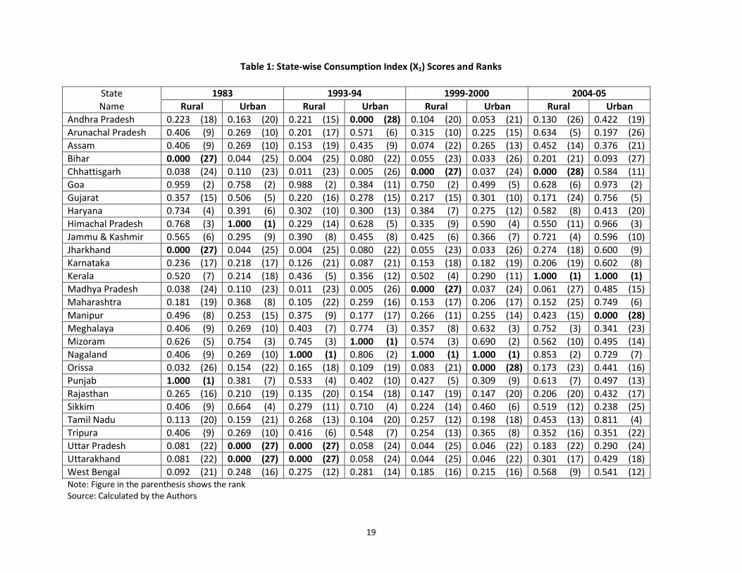
State-wise Consumption Index (X1), generated by following the methodology

described earlier is reported in Table 1. It is observed from the table that Kerala, Goa,

Himachal, Tamil Nadu and Gujarat are among the toppers in terms of urban

consumption in 2004-05, while Arunachal Pradesh, Bihar, Manipur and Sikkim are at the

bottom. The stark difference in terms of consumption pattern within states becomes

quite clear from the table. For instance in 2004-05, while Arunachal Pradesh ranks 26th

in terms of urban consumption, it is ranked 5th

in terms of rural consumption scores. On

the other hand in the same year, while Tamil Nadu ranks 4th

in terms of urban

consumption, it is ranked 13th

in terms of rural consumption scores. The comparison of

rankings of the states over the period reveals that the relative position of the states has

witnessed varying changes over the period. For instance, while Kerala’s ranking has

improved and the same for Haryana has deteriorated over 1983-2005.

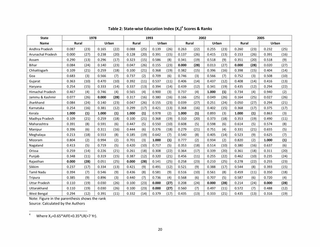
Table 2 reports the state-wise scenario on education index (X2). Like the case of

consumption, the states have witnessed differing level of success in the urban and rural

belt. For instance in 2004-05, Assam obtains 9th

ranking in terms of urban educational

achievements, but it is in 20th

position in terms of performance in the rural belt. On the

whole, Mizoram, Kerala, Himachal Pradesh, Tripura etc. are among the toppers, while

UP, Bihar, Jammu and Kashmir are at the other end of the spectrum. It is observed that

states like Tamil Nadu slide down the ladder over 1983-2005.

10

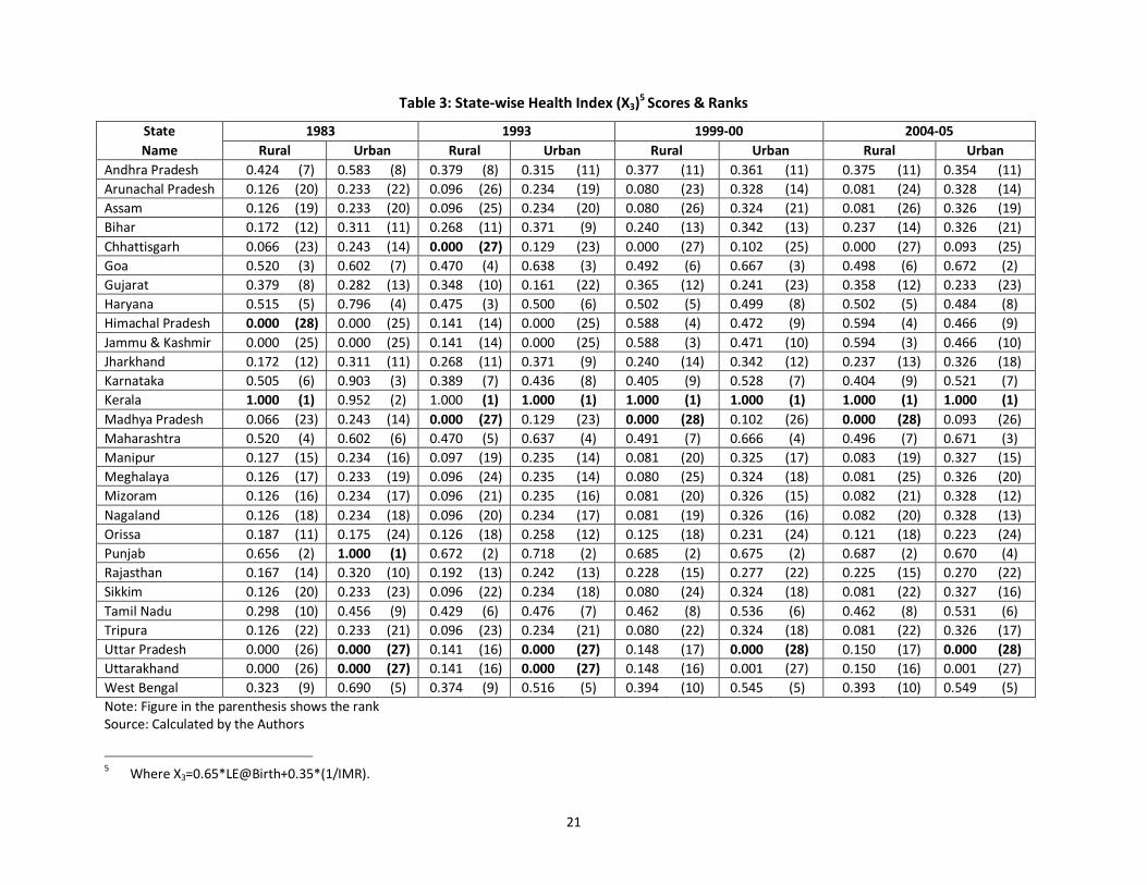
Table 3 shows the state-wise health Index (X3) for the four periods under

consideration. Intra-state divergence in terms of achievements is found to be the

defining feature in this front as well. For instance in 2004-05, while Gujarat ranks 23rd

in

terms of urban health achievements, it is ranked 12th

in terms of rural health scores.

Looking at the overall performance in 2004-05, it is observed that Kerala, Goa, Punjab

are among the toppers, while Chhattisgarh and Madhya Pradesh are at the bottom. By

comparing the 1983 and 2004-05 performance of the states, it is observed that

Himachal Pradesh and Jammu and Kashmir have improved their performance

commendably, while Gujarat has witnessed a declined both in the terms of rural and

urban rankings.

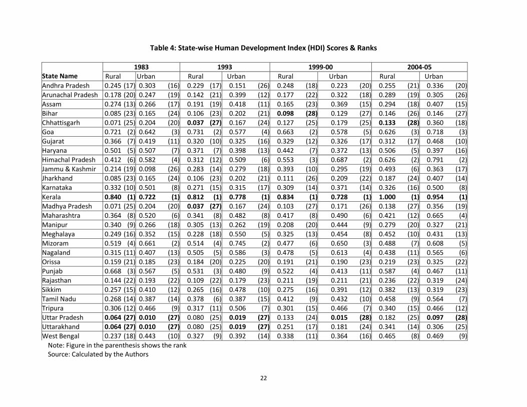
The overall HD scores for the states generated following the above methodology

is presented in Table 4. It is observed from the table that HD level is consistently high for

states like Kerala, Goa, Mizoram, Himachal Pradesh etc., who are otherwise performing

well in constituent categories. On the other hand, Chhattisgarh, Uttar Pradesh,

Uttarakhand, Bihar, Orissa etc. have always been among the bottom liners. Some

interesting movement across the states is noticed over the period of analysis. For

instance, Punjab and Haryana start with an appreciable HD scenario in 1983, but their

performance in the urban areas decline considerably during the last period. A similar

worsening effect is noticed for Arunachal Pradesh at the bottom as well. On the other

hand, Jammu & Kashmir and West Bengal has managed to improve their HD level to

some extent over the period. Interestingly Jharkhand has shown marked improvement

in terms of HD achievements after separation from Bihar.

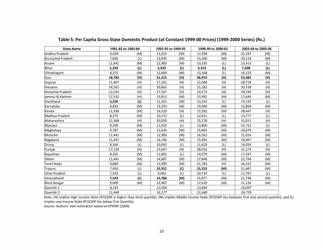
The changing income scenario across the states is explained with the help of

Table 5. The income quartiles during the years under observation are defined and the

states falling under different income categories during a period are mentioned in the

parenthesis. It is observed from the table that while Punjab, Haryana, Goa, Gujarat and

Maharashtra remained in the high income category throughout the period, Bihar, Orisa

11

and Uttar Pradesh stayed on the other extreme. States witnessing a growth in the

service sector of late, i.e., Andhra Pradesh, Karnataka, Tamil Nadu and West Bengal

remained in the mid-income category. The position of Kerala kept fluctuating between

high and middle-income category. A fluctuating trend between low and middle-income

category is noticed for some Northeastern states as well. It becomes clear that

liberalisation exercise has affected the growth path of the states in different manner.

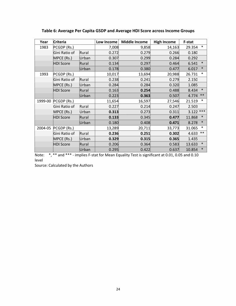
Before exploring the relationship between HD and EG, a deeper analysis on the

quality of income growth across Indian states would not be irrelevant here. The concern

here is that the inequality in the growth process may adversely influence the pace of HD

formation in a state. Table 6 compares the HD level of the states in the rural and the

urban belt with the respective Gini ratios. It is observed from the table that the rise in

income level over the study period is associated with rise in inequality in the high

income states during 1983 to 1993 (both for rural and urban). For high income states,

the inequality marginally fall (both for rural and urban) during 1993 to 1999-00, but

again gone up during 1999-00 to 2004-05. Except for urban areas under low income

states during 1993 to 1999-00, the inequality (both for rural and urban) gradually

declined during 1983 to 1999-00. However, urban inequality is found to be gone up for

low income States during 1993 to 1999-00. For all income states, both for rural and

urban, the inequality has gone up during 1999-00 to 2004-05.

Understandably, the increase in the HDI score for the low income states over

1983 to 2004-05 has been moderate as compared to the corresponding figures for the

high-income states. Average HDI score of the States is significantly different across

income categories. The existing literature suggests that the rising inequality has affected

the growth process and livelihood of the citizens of different states differently, though

HD level has improved across all income groups. However, the improvement is not

smooth. For middle income States, both for rural and urban, HDI score in 1993 is lower

than 1983. For lower income States, for urban areas, HDI score in 1999-00 is lower than

12

1993 and for high income States, for rural and urban, the HDI score in 1999-00 is lower

than 1993.

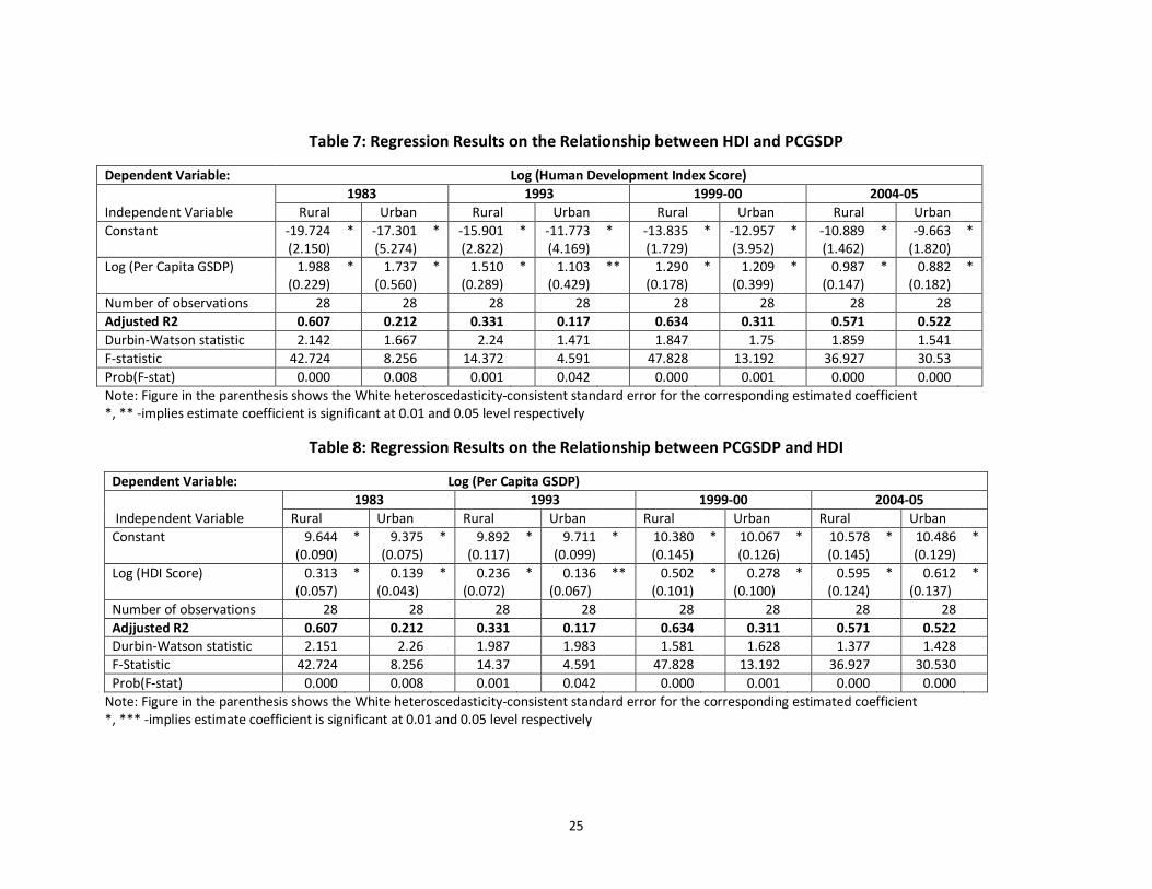
Finally, in order to understand the relationship between EG and HD, a regression

analysis has been undertaken, involving the logarithm of the HDI score as dependent

variable and the logarithm of the PCGSDP of the states as independent variable. The

cross-section regressions are separately estimated for the four periods under study. In

addition to capture the rural-urban divergence, separate regression models are

estimated on that account as well.

It is observed from the results reported in Table 7 that the HDI formation process

of the states is positively influenced by the growing income levels, as reflected from the

positive value and significance level of the coefficients of logarithms of Per Capita GSDP

for all four periods and for rural and urban areas. However, a point of concern is that

the value of the coefficients of the log (PCGSDP) (which measures the income elasticity

of human development), both for rural and urban areas, is declining over the period.

The result implies that per capita income (as an indicator of economic growth) is not

translating into human well being. This perhaps in another way might signify the rising

influence of other variables in determination of the HD achievements of a state. The

result shows the need for further investigation to determine the underlying factors

(other than per capita income) which influence HD achievements of a State. Another

interesting observation is worth mention here. For all the years the income elasticity of

human development is higher for rural areas as compared to urban areas. This implies

that an increase in per capita income results higher human development in rural areas

as compared to their urban counterparts, which underlines the importance of the

schemes like NREGA in no uncertain terms.

A second set of regression is undertaken involving the logarithm of PCGSDP as

dependent variable and the logarithm of the HDI score of the states as independent

13

variable, to understand the dependence pattern the other way round. The regression

results reported in Table 8 shows that HD significantly influences EG level of a state.

Looking at the coefficients of the logarithmic transformation of HDI, it is observed that

before 1999-00, the HD elasticity of EG was smaller and the rural HD is found to

influence EG in a more significant manner as compared to urban HD. However, in 2004-

05, urban HD surpasses the rural HD level in influencing EG. Larger influence of HD on

EG in recent period suggests that investment in HD will have larger impact on EG, and

hence the long run implications of introducing SSA and NRHM becomes all the more

important.

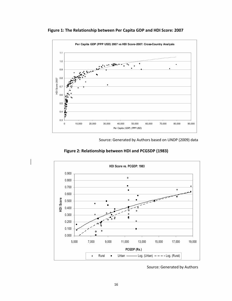
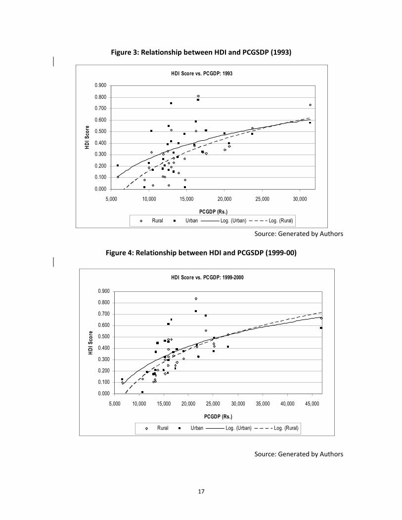
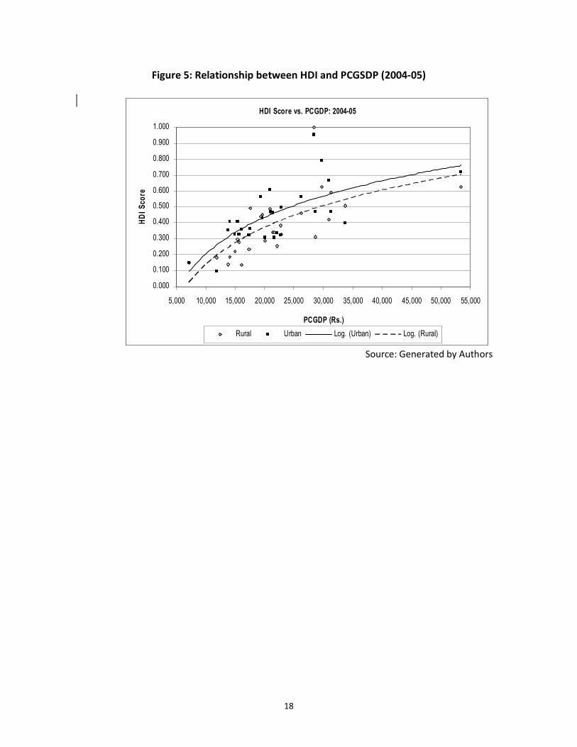
Figures 2-5 pictorially depict the cross-state relationship between HD and EG

during the four periods under observation across the states. The rural and urban income

levels and HD achievements are considered separately in the diagrams. A couple of

observations emerge from the figures. First, the positive relationship between EG and

HD holds good for all four periods under consideration. Second, the relationship

between EG and HD is non-linear in nature; rising level of income is associated with

lesser degree of increase in terms of HD achievements beyond a critical level. Third,

despite rising income inequality in the last period under consideration (2004-05), as

reflected from the divergence of the rural and urban curves, this non-linear structural

relationship is not affected in any significant manner. Except for a few States, the urban

HDI score is generally higher than rural HDI score for all the periods of our analysis. For

instance in case of Goa, a high income State, rural HDI score is higher than urban HDI

score for 1983, 1993 and 1999, but an opposite scenario emerges in 2004-05. On the

other hand, for high income states like Punjab and Haryana (1999-00, 2004-05), rural

HDI score is higher than urban HDI score. The same is true for middle income States like

Kerala, Jammu & Kashmir, Andhra Pradesh (1993, 1999-00) as well as low income States

Uttar Pradesh and Uttarakhand.

14

Over the last decade the contribution of the service sector in India’s GDP has

increased tremendously. Health and education sector are part to that growth trajectory

in a two-way process: on one hand they form part of the service sector, and on the

other hand healthy and educated population stand to augment the GDP in a more

productive manner not only in the service sector but also within agriculture and

manufacturing segment. It is observed from the current analysis that EG and HD levels

in India are positively related, and the relationship works in both directions. While this is

a comforting observation, indirectly implying that the HD formation process resulting

from the rising income level in the current period would continue to provide growth

impetus in the subsequent period, the rising inequality level in the recent period is a

major area of concern. One important policy response for the Government would

therefore be to ensure a balanced growth process across the states on one hand, and to

bridge the gap between the rural and urban areas within a state on the other. Only then

the benefits of the EG and HD augmentation process would cumulatively lead to

sustainable economic development path.

Last but not the least, the role of governance and institutions is important to

translate the economic growth into economic development. There are several routes

through which economic growth could influence economic development, but the most

obvious route where government policies and institutions could play an important role

is through economic growth – tax revenue generation of the governments and

expenditure on social sector and developmental activities. Higher economic growth will

result in larger tax revenue generations to the State governments which could provide

larger fiscal space for State governments to spend on social sector programmes and

developmental activities. It is expected that States having higher tax-GSDP ratio have

larger fiscal space to translate economic growth into economic development. However,

States having larger outstanding debt leave with eroded fiscal space as a substantial part

of revenue goes to debt-financing (Chakraborty et al., 2009). It is the low per capita

income States who have larger outstanding public debt as compared high and middle

15

income States (see Chakraborty et al., 2009). Apart from State governments’

expenditure on social sectors, there are several centrally sponsored schemes are

running on social sectors which could help substantially to translate economic growth

into economic development. A recent study shows that transferred to fund under

centrally sponsored schemes to states is regressive (Chakraborty et al., 2010). As a

result, in absence of adequate fiscal space to States it would be over ambitious to

expect automatic translation of economic growth into economic development.

16

��

��

��

��

��

��

��

��

��

��

��

��

��

��

��

��

��

Per Capita GDP (PPP USD) 2007 vs HDI Score-2007: Cross-Country Analysis

0.3

0.4

0.5

0.6

0.7

0.8

0.9

1.0

1.1

0 10,000 20,000 30,000 40,000 50,000 60,000 70,000 80,000 90,000

Per Capita (GDP) (PPP USD)

HD

I S

core

-2007

Figure 1: The Relationship between Per Capita GDP and HDI Score: 2007

Source: Generated by Authors based on UNDP (2009) data

Figure 2: Relationship between HDI and PCGSDP (1983)

Source: Generated by Authors

17

��

��

��

��

��

��

��

��

��

��

��

��

��

��

��

��

��

��

��

��

��

��

��

��

��

��

��

��

��

��

��

��

��

��

Figure 3: Relationship between HDI and PCGSDP (1993)


Figure 4: Relationship between HDI and PCGSDP (1999-00)


18

��

��

��

��

��

��

��

��

��

��

��

��

��

��

��

��

��

��

Figure 5: Relationship between HDI and PCGSDP (2004-05)


19

Table 1: State-wise Consumption Index (X1) Scores and Ranks

State 1983 1993-94 1999-2000 2004-05

Name Rural Urban Rural Urban Rural Urban Rural Urban

Andhra Pradesh 0.223 (18) 0.163 (20) 0.221 (15) 0.000 (28) 0.104 (20) 0.053 (21) 0.130 (26) 0.422 (19)

Arunachal Pradesh 0.406 (9) 0.269 (10) 0.201 (17) 0.571 (6) 0.315 (10) 0.225 (15) 0.634 (5) 0.197 (26)

Assam 0.406 (9) 0.269 (10) 0.153 (19) 0.435 (9) 0.074 (22) 0.265 (13) 0.452 (14) 0.376 (21)

Bihar 0.000 (27) 0.044 (25) 0.004 (25) 0.080 (22) 0.055 (23) 0.033 (26) 0.201 (21) 0.093 (27)

Chhattisgarh 0.038 (24) 0.110 (23) 0.011 (23) 0.005 (26) 0.000 (27) 0.037 (24) 0.000 (28) 0.584 (11)

Goa 0.959 (2) 0.758 (2) 0.988 (2) 0.384 (11) 0.750 (2) 0.499 (5) 0.628 (6) 0.973 (2)

Gujarat 0.357 (15) 0.506 (5) 0.220 (16) 0.278 (15) 0.217 (15) 0.301 (10) 0.171 (24) 0.756 (5)

Haryana 0.734 (4) 0.391 (6) 0.302 (10) 0.300 (13) 0.384 (7) 0.275 (12) 0.582 (8) 0.413 (20)

Himachal Pradesh 0.768 (3) 1.000 (1) 0.229 (14) 0.628 (5) 0.335 (9) 0.590 (4) 0.550 (11) 0.966 (3)

Jammu & Kashmir 0.565 (6) 0.295 (9) 0.390 (8) 0.455 (8) 0.425 (6) 0.366 (7) 0.721 (4) 0.596 (10)

Jharkhand 0.000 (27) 0.044 (25) 0.004 (25) 0.080 (22) 0.055 (23) 0.033 (26) 0.274 (18) 0.600 (9)

Karnataka 0.236 (17) 0.218 (17) 0.126 (21) 0.087 (21) 0.153 (18) 0.182 (19) 0.206 (19) 0.602 (8)

Kerala 0.520 (7) 0.214 (18) 0.436 (5) 0.356 (12) 0.502 (4) 0.290 (11) 1.000 (1) 1.000 (1)

Madhya Pradesh 0.038 (24) 0.110 (23) 0.011 (23) 0.005 (26) 0.000 (27) 0.037 (24) 0.061 (27) 0.485 (15)

Maharashtra 0.181 (19) 0.368 (8) 0.105 (22) 0.259 (16) 0.153 (17) 0.206 (17) 0.152 (25) 0.749 (6)

Manipur 0.496 (8) 0.253 (15) 0.375 (9) 0.177 (17) 0.266 (11) 0.255 (14) 0.423 (15) 0.000 (28)

Meghalaya 0.406 (9) 0.269 (10) 0.403 (7) 0.774 (3) 0.357 (8) 0.632 (3) 0.752 (3) 0.341 (23)

Mizoram 0.626 (5) 0.754 (3) 0.745 (3) 1.000 (1) 0.574 (3) 0.690 (2) 0.562 (10) 0.495 (14)

Nagaland 0.406 (9) 0.269 (10) 1.000 (1) 0.806 (2) 1.000 (1) 1.000 (1) 0.853 (2) 0.729 (7)

Orissa 0.032 (26) 0.154 (22) 0.165 (18) 0.109 (19) 0.083 (21) 0.000 (28) 0.173 (23) 0.441 (16)

Punjab 1.000 (1) 0.381 (7) 0.533 (4) 0.402 (10) 0.427 (5) 0.309 (9) 0.613 (7) 0.497 (13)

Rajasthan 0.265 (16) 0.210 (19) 0.135 (20) 0.154 (18) 0.147 (19) 0.147 (20) 0.206 (20) 0.432 (17)

Sikkim 0.406 (9) 0.664 (4) 0.279 (11) 0.710 (4) 0.224 (14) 0.460 (6) 0.519 (12) 0.238 (25)

Tamil Nadu 0.113 (20) 0.159 (21) 0.268 (13) 0.104 (20) 0.257 (12) 0.198 (18) 0.453 (13) 0.811 (4)

Tripura 0.406 (9) 0.269 (10) 0.416 (6) 0.548 (7) 0.254 (13) 0.365 (8) 0.352 (16) 0.351 (22)

Uttar Pradesh 0.081 (22) 0.000 (27) 0.000 (27) 0.058 (24) 0.044 (25) 0.046 (22) 0.183 (22) 0.290 (24)

Uttarakhand 0.081 (22) 0.000 (27) 0.000 (27) 0.058 (24) 0.044 (25) 0.046 (22) 0.301 (17) 0.429 (18)

West Bengal 0.092 (21) 0.248 (16) 0.275 (12) 0.281 (14) 0.185 (16) 0.215 (16) 0.568 (9) 0.541 (12)

Note: Figure in the parenthesis shows the rank

Source: Calculated by the Authors

20

Table 2: State-wise Education Index (X2)4 Scores & Ranks



4 Where X2=0.65*AIFE+0.35*LR(>7 Yr).

State 1978 1993 2002 2005


Andhra Pradesh 0.087 (23) 0.165 (22) 0.088 (25) 0.139 (26) 0.263 (22) 0.255 (23) 0.260 (23) 0.232 (25)


Assam 0.290 (13) 0.296 (17) 0.323 (15) 0.586 (8) 0.341 (19) 0.518 (9) 0.351 (20) 0.518 (9)

Bihar 0.084 (24) 0.140 (23) 0.047 (26) 0.155 (23) 0.000 (28) 0.013 (27) 0.000 (28) 0.020 (27)

Chhattisgarh 0.109 (21) 0.259 (18) 0.100 (21) 0.368 (19) 0.382 (15) 0.396 (16) 0.398 (15) 0.404 (14)

Goa 0.683 (3) 0.566 (7) 0.737 (2) 0.709 (6) 0.746 (3) 0.566 (7) 0.752 (3) 0.508 (10)

Gujarat 0.363 (10) 0.470 (10) 0.392 (11) 0.537 (11) 0.406 (14) 0.437 (12) 0.408 (14) 0.416 (13)

Haryana 0.254 (15) 0.333 (14) 0.337 (13) 0.394 (14) 0.439 (12) 0.341 (19) 0.435 (12) 0.294 (22)


Jammu & Kashmir 0.077 (26) 0.000 (28) 0.317 (16) 0.380 (16) 0.166 (25) 0.049 (26) 0.164 (25) 0.027 (26)

Jharkhand 0.084 (24) 0.140 (23) 0.047 (26) 0.155 (23) 0.039 (27) 0.251 (24) 0.050 (27) 0.294 (21)

Karnataka 0.254 (16) 0.381 (12) 0.299 (17) 0.421 (13) 0.368 (16) 0.402 (15) 0.368 (17) 0.375 (17)

Kerala 1.000 (1) 1.000 (1) 1.000 (1) 0.978 (2) 1.000 (1) 0.893 (3) 1.000 (1) 0.863 (3)

Madhya Pradesh 0.109 (21) 0.259 (18) 0.100 (21) 0.368 (19) 0.310 (20) 0.373 (18) 0.353 (19) 0.490 (11)

Maharashtra 0.391 (8) 0.591 (6) 0.447 (5) 0.550 (10) 0.608 (5) 0.598 (6) 0.614 (5) 0.574 (8)

Manipur 0.396 (6) 0.311 (16) 0.444 (6) 0.376 (18) 0.279 (21) 0.751 (4) 0.331 (21) 0.655 (5)

Meghalaya 0.213 (18) 0.553 (8) 0.185 (19) 0.642 (7) 0.540 (8) 0.405 (14) 0.523 (9) 0.625 (7)

Mizoram 0.804 (2) 0.994 (2) 0.701 (3) 1.000 (1) 0.777 (2) 0.934 (2) 0.820 (2) 1.000 (1)

Nagaland 0.413 (5) 0.719 (5) 0.420 (10) 0.717 (5) 0.353 (18) 0.514 (10) 0.380 (16) 0.637 (6)

Orissa 0.259 (14) 0.226 (21) 0.261 (18) 0.308 (22) 0.364 (17) 0.339 (20) 0.361 (18) 0.311 (20)

Punjab 0.348 (11) 0.319 (15) 0.387 (12) 0.320 (21) 0.456 (11) 0.255 (22) 0.462 (10) 0.235 (24)

Rajasthan 0.000 (28) 0.051 (25) 0.000 (28) 0.141 (25) 0.258 (23) 0.210 (25) 0.278 (22) 0.255 (23)

Sikkim 0.237 (17) 0.334 (13) 0.421 (9) 0.491 (12) 0.521 (9) 0.388 (17) 0.544 (8) 0.393 (15)

Tamil Nadu 0.394 (7) 0.546 (9) 0.436 (8) 0.581 (9) 0.516 (10) 0.561 (8) 0.459 (11) 0.350 (18)

Tripura 0.385 (9) 0.896 (3) 0.440 (7) 0.736 (4) 0.568 (6) 0.707 (5) 0.587 (6) 0.720 (4)

Uttar Pradesh 0.110 (19) 0.030 (26) 0.100 (23) 0.000 (27) 0.208 (24) 0.000 (28) 0.214 (24) 0.000 (28)

Uttarakhand 0.110 (19) 0.030 (26) 0.100 (23) 0.000 (27) 0.560 (7) 0.497 (11) 0.572 (7) 0.488 (12)

West Bengal 0.294 (12) 0.391 (11) 0.332 (14) 0.379 (17) 0.435 (13) 0.333 (21) 0.435 (13) 0.316 (19)

21

Table 3: State-wise Health Index (X3)5

Scores & Ranks

State 1983 1993 1999-00 2004-05


Andhra Pradesh 0.424 (7) 0.583 (8) 0.379 (8) 0.315 (11) 0.377 (11) 0.361 (11) 0.375 (11) 0.354 (11)


Assam 0.126 (19) 0.233 (20) 0.096 (25) 0.234 (20) 0.080 (26) 0.324 (21) 0.081 (26) 0.326 (19)

Bihar 0.172 (12) 0.311 (11) 0.268 (11) 0.371 (9) 0.240 (13) 0.342 (13) 0.237 (14) 0.326 (21)

Chhattisgarh 0.066 (23) 0.243 (14) 0.000 (27) 0.129 (23) 0.000 (27) 0.102 (25) 0.000 (27) 0.093 (25)

Goa 0.520 (3) 0.602 (7) 0.470 (4) 0.638 (3) 0.492 (6) 0.667 (3) 0.498 (6) 0.672 (2)

Gujarat 0.379 (8) 0.282 (13) 0.348 (10) 0.161 (22) 0.365 (12) 0.241 (23) 0.358 (12) 0.233 (23)

Haryana 0.515 (5) 0.796 (4) 0.475 (3) 0.500 (6) 0.502 (5) 0.499 (8) 0.502 (5) 0.484 (8)


Jammu & Kashmir 0.000 (25) 0.000 (25) 0.141 (14) 0.000 (25) 0.588 (3) 0.471 (10) 0.594 (3) 0.466 (10)

Jharkhand 0.172 (12) 0.311 (11) 0.268 (11) 0.371 (9) 0.240 (14) 0.342 (12) 0.237 (13) 0.326 (18)

Karnataka 0.505 (6) 0.903 (3) 0.389 (7) 0.436 (8) 0.405 (9) 0.528 (7) 0.404 (9) 0.521 (7)

Kerala 1.000 (1) 0.952 (2) 1.000 (1) 1.000 (1) 1.000 (1) 1.000 (1) 1.000 (1) 1.000 (1)

Madhya Pradesh 0.066 (23) 0.243 (14) 0.000 (27) 0.129 (23) 0.000 (28) 0.102 (26) 0.000 (28) 0.093 (26)

Maharashtra 0.520 (4) 0.602 (6) 0.470 (5) 0.637 (4) 0.491 (7) 0.666 (4) 0.496 (7) 0.671 (3)

Manipur 0.127 (15) 0.234 (16) 0.097 (19) 0.235 (14) 0.081 (20) 0.325 (17) 0.083 (19) 0.327 (15)

Meghalaya 0.126 (17) 0.233 (19) 0.096 (24) 0.235 (14) 0.080 (25) 0.324 (18) 0.081 (25) 0.326 (20)

Mizoram 0.126 (16) 0.234 (17) 0.096 (21) 0.235 (16) 0.081 (20) 0.326 (15) 0.082 (21) 0.328 (12)

Nagaland 0.126 (18) 0.234 (18) 0.096 (20) 0.234 (17) 0.081 (19) 0.326 (16) 0.082 (20) 0.328 (13)

Orissa 0.187 (11) 0.175 (24) 0.126 (18) 0.258 (12) 0.125 (18) 0.231 (24) 0.121 (18) 0.223 (24)

Punjab 0.656 (2) 1.000 (1) 0.672 (2) 0.718 (2) 0.685 (2) 0.675 (2) 0.687 (2) 0.670 (4)

Rajasthan 0.167 (14) 0.320 (10) 0.192 (13) 0.242 (13) 0.228 (15) 0.277 (22) 0.225 (15) 0.270 (22)

Sikkim 0.126 (20) 0.233 (23) 0.096 (22) 0.234 (18) 0.080 (24) 0.324 (18) 0.081 (22) 0.327 (16)

Tamil Nadu 0.298 (10) 0.456 (9) 0.429 (6) 0.476 (7) 0.462 (8) 0.536 (6) 0.462 (8) 0.531 (6)

Tripura 0.126 (22) 0.233 (21) 0.096 (23) 0.234 (21) 0.080 (22) 0.324 (18) 0.081 (22) 0.326 (17)

Uttar Pradesh 0.000 (26) 0.000 (27) 0.141 (16) 0.000 (27) 0.148 (17) 0.000 (28) 0.150 (17) 0.000 (28)

Uttarakhand 0.000 (26) 0.000 (27) 0.141 (16) 0.000 (27) 0.148 (16) 0.001 (27) 0.150 (16) 0.001 (27)

West Bengal 0.323 (9) 0.690 (5) 0.374 (9) 0.516 (5) 0.394 (10) 0.545 (5) 0.393 (10) 0.549 (5)



5 Where X3=0.65*LE@Birth+0.35*(1/IMR).

22

Table 4: State-wise Human Development Index (HDI) Scores & Ranks

1983 1993 1999-00 2004-05

State Name Rural Urban Rural Urban Rural Urban Rural Urban

Andhra Pradesh 0.245 (17) 0.303 (16) 0.229 (17) 0.151 (26) 0.248 (18) 0.223 (20) 0.255 (21) 0.336 (20)


Assam 0.274 (13) 0.266 (17) 0.191 (19) 0.418 (11) 0.165 (23) 0.369 (15) 0.294 (18) 0.407 (15)

Bihar 0.085 (23) 0.165 (24) 0.106 (23) 0.202 (21) 0.098 (28) 0.129 (27) 0.146 (26) 0.146 (27)

Chhattisgarh 0.071 (25) 0.204 (20) 0.037 (27) 0.167 (24) 0.127 (25) 0.179 (25) 0.133 (28) 0.360 (18)

Goa 0.721 (2) 0.642 (3) 0.731 (2) 0.577 (4) 0.663 (2) 0.578 (5) 0.626 (3) 0.718 (3)

Gujarat 0.366 (7) 0.419 (11) 0.320 (10) 0.325 (16) 0.329 (12) 0.326 (17) 0.312 (17) 0.468 (10)

Haryana 0.501 (5) 0.507 (7) 0.371 (7) 0.398 (13) 0.442 (7) 0.372 (13) 0.506 (5) 0.397 (16)


Jammu & Kashmir 0.214 (19) 0.098 (26) 0.283 (14) 0.279 (18) 0.393 (10) 0.295 (19) 0.493 (6) 0.363 (17)

Jharkhand 0.085 (23) 0.165 (24) 0.106 (23) 0.202 (21) 0.111 (26) 0.209 (22) 0.187 (24) 0.407 (14)

Karnataka 0.332 (10) 0.501 (8) 0.271 (15) 0.315 (17) 0.309 (14) 0.371 (14) 0.326 (16) 0.500 (8)

Kerala 0.840 (1) 0.722 (1) 0.812 (1) 0.778 (1) 0.834 (1) 0.728 (1) 1.000 (1) 0.954 (1)

Madhya Pradesh 0.071 (25) 0.204 (20) 0.037 (27) 0.167 (24) 0.103 (27) 0.171 (26) 0.138 (27) 0.356 (19)

Maharashtra 0.364 (8) 0.520 (6) 0.341 (8) 0.482 (8) 0.417 (8) 0.490 (6) 0.421 (12) 0.665 (4)

Manipur 0.340 (9) 0.266 (18) 0.305 (13) 0.262 (19) 0.208 (20) 0.444 (9) 0.279 (20) 0.327 (21)

Meghalaya 0.249 (16) 0.352 (15) 0.228 (18) 0.550 (5) 0.325 (13) 0.454 (8) 0.452 (10) 0.431 (13)

Mizoram 0.519 (4) 0.661 (2) 0.514 (4) 0.745 (2) 0.477 (6) 0.650 (3) 0.488 (7) 0.608 (5)

Nagaland 0.315 (11) 0.407 (13) 0.505 (5) 0.586 (3) 0.478 (5) 0.613 (4) 0.438 (11) 0.565 (6)

Orissa 0.159 (21) 0.185 (23) 0.184 (20) 0.225 (20) 0.191 (21) 0.190 (23) 0.219 (23) 0.325 (22)

Punjab 0.668 (3) 0.567 (5) 0.531 (3) 0.480 (9) 0.522 (4) 0.413 (11) 0.587 (4) 0.467 (11)

Rajasthan 0.144 (22) 0.193 (22) 0.109 (22) 0.179 (23) 0.211 (19) 0.211 (21) 0.236 (22) 0.319 (24)

Sikkim 0.257 (15) 0.410 (12) 0.265 (16) 0.478 (10) 0.275 (16) 0.391 (12) 0.382 (13) 0.319 (23)

Tamil Nadu 0.268 (14) 0.387 (14) 0.378 (6) 0.387 (15) 0.412 (9) 0.432 (10) 0.458 (9) 0.564 (7)

Tripura 0.306 (12) 0.466 (9) 0.317 (11) 0.506 (7) 0.301 (15) 0.466 (7) 0.340 (15) 0.466 (12)

Uttar Pradesh 0.064 (27) 0.010 (27) 0.080 (25) 0.019 (27) 0.133 (24) 0.015 (28) 0.182 (25) 0.097 (28)

Uttarakhand 0.064 (27) 0.010 (27) 0.080 (25) 0.019 (27) 0.251 (17) 0.181 (24) 0.341 (14) 0.306 (25)

West Bengal 0.237 (18) 0.443 (10) 0.327 (9) 0.392 (14) 0.338 (11) 0.364 (16) 0.465 (8) 0.469 (9)



23

Table 5: Per Capita Gross State Domestic Product (at Constant 1999-00 Prices) (1999-2000 Series) (Rs.)

State Name 1981-82 to 1983-84 1992-93 to 1994-95 1998-99 to 2000-01 2003-04 to 2005-06

Andhra Pradesh 9,439 (M) 13,252 (M) 17,358 (M) 22,247 (M)

Arunachal Pradesh 7,836 (L) 13,935 (M) 15,246 (M) 20,119 (M)

Assam 11,441 (M) 12,983 (M) 13,335 (L) 15,413 (L)

Bihar 5,259 (L) 5,929 (L) 6,553 (L) 7,208 (L)

Chhattisgarh 8,275 (M) 12,600 (M) 13,168 (L) 16,225 (M)

Goa 18,782 (H) 31,315 (H) 46,919 (H) 53,485 (H)

Gujarat 11,467 (H) 17,101 (H) 22,068 (H) 28,719 (H)

Haryana 14,501 (H) 20,662 (H) 25,182 (H) 33,728 (H)

Himachal Pradesh 12,554 (H) 17,567 (H) 23,573 (H) 29,749 (H)

Jammu & Kashmir 12,332 (H) 13,815 (M) 15,992 (M) 17,644 (M)

Jharkhand 5,259 (L) 12,101 (M) 13,245 (L) 14,192 (L)

Karnataka 8,832 (M) 13,253 (M) 19,090 (M) 22,858 (M)

Kerala 11,336 (M) 16,520 (H) 21,592 (M) 28,447 (H)

Madhya Pradesh 8,275 (M) 10,572 (L) 12,911 (L) 13,777 (L)

Maharashtra 12,368 (H) 20,050 (H) 25,278 (H) 31,011 (H)

Manipur 9,296 (M) 11,922 (L) 13,800 (M) 15,712 (L)

Meghalaya 9,787 (M) 12,634 (M) 15,963 (M) 19,679 (M)

Mizoram 11,441 (M) 12,983 (M) 16,562 (M) 21,014 (M)

Nagaland 11,441 (M) 16,196 (M) 15,992 (M) 19,467 (M)

Orissa 8,164 (L) 10,042 (L) 11,629 (L) 14,924 (L)

Punjab 17,134 (H) 23,697 (H) 28,016 (H) 31,273 (H)

Rajasthan 8,202 (M) 11,842 (L) 14,979 (M) 17,337 (M)

Sikkim 11,441 (M) 14,687 (M) 17,648 (M) 22,794 (M)

Tamil Nadu 9,800 (M) 15,999 (M) 21,783 (H) 26,222 (M)

Tripura 7,456 (L) 10,351 (L) 15,255 (M) 21,487 (M)

Uttar Pradesh 7,543 (L) 9,460 (L) 10,734 (L) 11,797 (L)

Uttarakhand 7,543 (L) 14,786 (M) 15,877 (M) 21,738 (M)

West Bengal 9,009 (M) 12,487 (M) 17,010 (M) 21,126 (M)

Quartile 1 8,193 12,056 13,684 16,097

Quartile 3 11,448 16,277 21,640 26,778

Note: (H) implies High Income State (PCGSDP is higher than third quartile); (M) implies Middle Income State (PCGSDP lies between first and second quartile); and (L)

implies Low Income State (PCGSDP lies below First Quartile).

Source: Authors’ own estimation based on EPWRF (2009)

24

Table 6: Average Per Capita GSDP and Average HDI Score across Income Groups

Year Criteria Low Income Middle Income High Income F-stat

1983 PCGDP (Rs.) 7,008 9,858 14,163 29.354 *

Gini Ratio of Rural 0.272 0.279 0.266 0.180

MPCE (Rs.) Urban 0.307 0.299 0.284 0.292

HDI Score Rural 0.134 0.297 0.464 6.541 *

Urban 0.178 0.380 0.477 6.017 *

1993 PCGDP (Rs.) 10,017 13,694 20,988 26.731 *


MPCE (Rs.) Urban 0.284 0.284 0.320 1.085

HDI Score Rural 0.163 0.254 0.488 8.434 *

Urban 0.223 0.363 0.507 4.774 **

1999-00 PCGDP (Rs.) 11,654 16,597 27,546 21.519 *


MPCE (Rs.) Urban 0.313 0.273 0.311 3.122 ***

HDI Score Rural 0.133 0.345 0.477 11.868 *

Urban 0.180 0.408 0.471 8.278 *

2004-05 PCGDP (Rs.) 13,289 20,711 33,773 31.065 *

Gini Ratio of Rural 0.236 0.251 0.302 4.633 **

MPCE (Rs.) Urban 0.329 0.315 0.365 1.435

HDI Score Rural 0.206 0.364 0.583 13.633 *

Urban 0.295 0.422 0.637 10.854 *

Note: *, ** and *** - implies F-stat for Mean Equality Test is significant at 0.01, 0.05 and 0.10

level


25

Table 7: Regression Results on the Relationship between HDI and PCGSDP

Dependent Variable: Log (Human Development Index Score)

1983 1993 1999-00 2004-05

Independent Variable Rural Urban Rural Urban Rural Urban Rural Urban

Constant -19.724 * -17.301 * -15.901 * -11.773 * -13.835 * -12.957 * -10.889 * -9.663 *

(2.150) (5.274) (2.822) (4.169) (1.729) (3.952) (1.462) (1.820)

Log (Per Capita GSDP) 1.988 * 1.737 * 1.510 * 1.103 ** 1.290 * 1.209 * 0.987 * 0.882 *

(0.229) (0.560) (0.289) (0.429) (0.178) (0.399) (0.147) (0.182)

Number of observations 28 28 28 28 28 28 28 28

Adjusted R2 0.607 0.212 0.331 0.117 0.634 0.311 0.571 0.522

Durbin-Watson statistic 2.142 1.667 2.24 1.471 1.847 1.75 1.859 1.541

F-statistic 42.724 8.256 14.372 4.591 47.828 13.192 36.927 30.53

Prob(F-stat) 0.000 0.008 0.001 0.042 0.000 0.001 0.000 0.000

Note: Figure in the parenthesis shows the White heteroscedasticity-consistent standard error for the corresponding estimated coefficient

*, ** -implies estimate coefficient is significant at 0.01 and 0.05 level respectively

Table 8: Regression Results on the Relationship between PCGSDP and HDI

Dependent Variable: Log (Per Capita GSDP)

1983 1993 1999-00 2004-05

Independent Variable Rural Urban Rural Urban Rural Urban Rural Urban

Constant 9.644 * 9.375 * 9.892 * 9.711 * 10.380 * 10.067 * 10.578 * 10.486 *

(0.090) (0.075) (0.117) (0.099) (0.145) (0.126) (0.145) (0.129)

Log (HDI Score) 0.313 * 0.139 * 0.236 * 0.136 ** 0.502 * 0.278 * 0.595 * 0.612 *

(0.057) (0.043) (0.072) (0.067) (0.101) (0.100) (0.124) (0.137)

Number of observations 28 28 28 28 28 28 28 28

Adjjusted R2 0.607 0.212 0.331 0.117 0.634 0.311 0.571 0.522

Durbin-Watson statistic 2.151 2.26 1.987 1.983 1.581 1.628 1.377 1.428

F-Statistic 42.724 8.256 14.37 4.591 47.828 13.192 36.927 30.530

Prob(F-stat) 0.000 0.008 0.001 0.042 0.000 0.001 0.000 0.000

Note: Figure in the parenthesis shows the White heteroscedasticity-consistent standard error for the corresponding estimated coefficient

*, *** -implies estimate coefficient is significant at 0.01 and 0.05 level respectively

26

References

Amin, A.A. (undated), “Economic Growth and Human Development with Capabilities

Expansion”, available at http://www-3.unipv.it/deontica/sen/papers/Amin.pdf (last

accessed on May 10, 2010).

Boozer, M., G. Ranis, F. Stewart and T. Suri (2003), “Path to Success: The relationship between

human development and economic growth”, Discussion Paper No. 874, Economic Growth

Center, Yale University.

Chakraborty, Pinaki, Anit Nath Mukherjee and H.K. Amar Nath (2010), “Interstate Distribution of

Central Expenditure and Subsidies”, Working Paper No. 2010-66, National Institute of Public

Finance and Policy, New Delhi.

Chakraborty, Pinaki, Anit Nath Mukherjee and H.K. Amar Nath (2009), “Macro Policy Reform and

Sub-National Finance: Why Is the Fiscal Space of the States Shrinking?”, Economic and

Political Weekly, Vol. XLVI, No. 14, pp. 38-44, April 04, 2009.

Chamarbagwala, Rubina (2009), “Economic liberalization and urban-rural inequality in India: a

quintile regression analysis”, Empirical Economics (forthcoming).

Costantini, Valeria and Salvatore Monni (2008), “Environment, human development and

economic growth”, Ecological Economics, Vol. 64, No. 4, pp. 867-880.

EPWRF (2009), “Domestic Product of States of India: 1960-61 to 2006-07”, EPWRF, Mumbai.

Ghosh, M. (2006) “Economic growth and human development in Indian States”, Economic and

Political Weekly, Vol. 41, No. 30, pp.3321–3329.

Government of India (undated), “Annual Report - 2007-08”, Department of School Education

and Literacy, Department of Education, Ministry of Human Resources Development,

Government of India, New Delhi.

Government of India (2002), “National Human Development Report 2001”, Planning

Commission, Government of India, New Delhi.

Guha, A. and D. Chakraborty (2003), “Relative Positions of Human Development Index Across

Indian States: Some Exploratory Results”, Artha Beekshan, Vol. 11, No. 4, pp. 166-181.

Himanshu (2009), “Towards new poverty lines for India”, Chapter 3 in Report of the Expert

Group to Review the Methodology for Estimation of Poverty, Planning Commission,

December 2009.

Joshi, Devin (2007), “The Relative Unimportance of Economic Growth for Human Development

in Developing Democracies: Cross-Sectional Evidence from the States of India”, Paper

presented at the 2007 Annual Meeting of the American Political Science Association, August

30th-September 2nd, 2007.

27

Mukherjee, S. and D. Chakraborty (2010), “Is there any Relationship between Environment,

Human Development, Political and Governance Regimes? Evidences from a Cross-Country

Analysis", MPRA Paper 19968, University Library of Munich, Germany.

Nagar, A.L., and Basu, S. R. (2001), “Weighing Socio-Economic Indicators of Human

Development: A Latent Variable Approach”, National Institute of Public Finance and Policy,

New Delhi.

NSSO (1986), “Levels and Pattern of Consumer Expenditure”, NSS 38th Round (January 1983 –

December 1983), NSSO, CSO, MoS&PI, GoI, New Delhi.

NSSO (1996), “Levels and Pattern of Consumer Expenditure”, NSS 50th Round (July 1993 - June

1994), Report No. 402, NSSO, CSO, MoS&PI, GoI, New Delhi.

NSSO (2002), “Levels and Pattern of Consumer Expenditure”, NSS 55th Round (July 1999 - June


NSSO (2007), “Levels and Pattern of Consumer Expenditure”, NSS 61st Round (July 2004 - June


Ranis, G. (2004), “Human development and economic growth”, Center Discussion Paper No. 887,

Economic Growth Center, Yale University, May, Available at:

http://www.econ.yale.edu/growth_pdf / cdp887.pdf (last accessed on April 7, 2010)

Ranis, G., F. Stewart and A. Ramirez (2000), “Economic Growth and Human Development”,

World Development, Vol. 28, No. 2, pp. 197-219.

Registrar General of India & Census Commissioner (2006), “Report of the Technical Group on

Population Projections Constituted by the National Commission on Population”, Registrar

General of India & Census Commissioner, Government of India, New Delhi.

Registrar General of India (1999), “Compendium of India’s Fertility and Mortality Indicators 1971

to 1997, based on Sample Registration System”, RGI, Government of India, New Delhi.

Registrar General of India (RGI) (2001), “Sample Registration System (SRS) Bulletin”, Volume 35,

No. 2, October 2001, RGI, Government of India, New Delhi.

United Nations Development Programme (UNDP) (2009), “Human Development Report 2009 -

Overcoming barriers: Human mobility and development”, New York: Palgrave Macmillan.

Documents

- Munich Personal RePEc Archive - Is there any relationship between … · 2019-09-26 · Munich Personal RePEc Archive Is there any relationship between Economic Growth and Human