MPRAMunich Personal RePEc Archive

Two Sides of a Medal: The ChangingRelationship between Religious Diversityand Religiosity

Matthias Opfinger

University Trier

September 2013

Online at https://mpra.ub.uni-muenchen.de/50152/MPRA Paper No. 50152, posted 30 September 2013 13:29 UTC

Two Sides of a Medal: The Changing Relationship between

Religious Diversity and Religiosity

Matthias Opfinger ∗

University Trier

Abstract

Religious Market Theory assigns basic market principles to the market for religion. The derived

supply side model proposes that religiosity is higher on a competitive market, characterized by high

religious diversity. Churches will provide higher quality goods compared to monopolistic churches.

The demand side model, originating from the Secularization Hypothesis, suggests that the establish-

ment of new churches casts doubt on the existing religion, which reduces overall religiosity. I find a

negative linear relationship between religious diversity and religiosity which supports the demand side

model. However, high levels of income, education, and democracy mitigate this effect. The relation-

ship becomes positive in the most developed countries. The demand side model seems to dominate

in less developed countries, while the supply side model better describes the market for religion after

Secularization has occurred.

JEL-classification: D4, O1, Z12

Keywords: Supply side, Demand side, interaction, attenuating effects

∗University Trier, Department of Economics. Universitaetsring 15, 54286 Trier, Germany. Phone: +49-(0)651-201 2714.Fax: +49-(0)651-201 3968. E-Mail: opfinger@uni-trier.de. I thank Ludwig von Auer, Claude Diebolt, Erich Gundlach,Martin Paldam, seminar participants in Hannover, and participants of the ACDD 2011 in Strasbourg for helpful commentson an earlier version.

1

1 Introduction

Religion is a good which is produced and supplied on markets. People in many of nowadays’ societies

are free to choose if they want to engage in religiosity and if so, in which faith they want to believe.

However, we can also observe that this freedom of choice is restricted in other countries or that adherence

to specific denominations is forbidden. At the same time, levels of religiosity appear to differ across the

world. Especially, the importance of religiosity seems to be lower in the Western and more developed

countries. The question arises whether there is a relationship between religious diversity and the level of

religiosity.

This question, or rather the possible answers to it, splits the scholars in this field of study in two camps.

On the one hand there is the Religious Market Theory, which is based on an influential article by Iannaccone

(1991). The market for religion is regarded similarly to any other market from a microeconomic perspective.

It follows that monopolistic churches want to increase profits which they achieve by reducing effort. The

quality of the produced good decreases, which leads to lower demand for this inferior good. Competition

between churches is promoted when religious diversity is high, that is, many different churches operate in

one country. These are forced to produce religion goods of high quality to attract more consumers to their

respective faith. The religious needs of the consumers are satisfied which raises their overall involvement

with religion. Consequently, this model implies that a large supply of religions goes along with higher

levels of religiosity.

On the other hand, the demand side model predicts a negative relationship between religious diversity

and religiosity. The argumentation is based on the Secularization Hypothesis which is prominent in the

social sciences, compare e.g. Martin (1978). Higher religious diversity induces believers to doubt the

correctness of their own faith, which weakens the ties with their respective denomination. Bar-El et al.

(2013) call this phenomenon disaffiliation and present a model of cultural transmission to investigate the

factors which influence the process of secularization. Instead of switching faiths, people reduce their overall

involvement with religion.

The aim of this analysis is to evaluate empirically the relationship between religious diversity and

religiosity without prior judgment of the underlying hypotheses. I want to derive conclusions on whether

the demand side or the supply side model of religion is better able to describe the market for religion.

It might appear to be a microeconomic problem as it would be interesting to see the effect of changing

religious diversity on one person’s religiosity. A similar approach is taken by Hanson and Xiang (2011)

who present a model to determine the market power of each religion. But unfortunately, religious diversity

and religiosity are rather slow moving variables. Consequently, I focus my analysis on the societal level

2

which means that I will compare different countries at different stages of economic development and with

different levels of religious diversity.

A main contribution of this analysis is that I extend the empirical estimations to investigate the factors

which mediate the role of religious diversity. I include interaction terms between the different explanatory

variables to measure if religious diversity might have different influences on religiosity, depending on the

stage of development. The results of this extension help to shed new light on the functioning of the market

for religion.

Furthermore, religiosity is measured differently and more comprehensively than in earlier studies. Most

studies use church attendance rates as a proxy variable for religious participation. This is obviously a

rather rough measure for actual religiosity as there might be many different reasons to go to church which

might not necessarily reflect actual religiosity. I will use a comprehensive measure of religiosity which is

proposed by Paldam and Gundlach (2012). They generate a measure of religiosity which is based on 14

different characteristics and people’s attitudes towards the church and faith itself. Interestingly, McCleary

and Barro (2006) only find a positive effect of religious diversity on religiosity when they use church

attendance rates as a proxy for religiosity. Using other measures related to religiosity, contained in Paldam

and Gundlach’s (2012) religiosity score, delivers inconclusive results. Glock and Stark (1965) also argue

against using church attendance rates as a measure for religiosity, stating that "[i]t is evident that to equate

the two [churchgoers] on the grounds of their actual participation in worship services is to obscure a major

difference in their involvement in ritualistic activity. This illustrates the inherent weakness of relying on a

single indicator to distinguish individuals on this, as well as other dimensions of religiosity."(p.29).

The results gained in this paper show that there is a negative relationship between religious diversity

and religiosity as proposed by the demand side model. The relationship between income and religiosity is

found to be negative as well which further supports the underlying Secularization Hypothesis. However, the

results on the interaction terms reveal that high levels of income, education, and democracy can mitigate

the negative influence of religious diversity on religiosity. The relationship even turns to positive for the

most developed countries. Apparently, the supply side model, derived from the Religious Market Theory

is a suitable description of the market for religion in the most developed societies.

The paper is organized as follows. The next Section will give an overview of the underlying Religious

Market Theory and the Secularization Hypothesis. Section 3 describes data and methodology. The results

are presented in Section 4 before they are discussed with regards to the underlying theories in Section 5.

Section 6 briefly concludes.

3

2 Theoretical Background

Iannaccone (1991) develops the Religious Market Theory by assigning basic microeconomic principles to

the market for religion. Monopolistic churches and their employees, similar to regular enterprises, try to

maximize their profits. However, the employees are civil servants and they are paid a fixed income by

the government. Hence their only possibility to increase profits is to reduce effort. The good which they

produce will be of minor quality, so that the demand for this inferior good declines. In contrast, churches

which operate in a competitive market cannot afford to produce goods of minor quality. They would loose

market shares and profits would decrease. This induces employees of churches in competitive markets to

exert optimal effort and raise the quality of their product. It follows that the demand for religion is higher

if different churches compete for the favor of the believers. In other words, higher religious diversity leads

to higher demand for religion goods which should be measurable as an increase in religiosity.

Iannaccone (1991) presents another argument in favor of a positive relationship between religious

diversity and religiosity. He states that monopolistic churches can only serve a fraction of people’s beliefs.

”[A single church] cannot be monotheistic and polytheistic; it cannot proclaim both that Jesus is the

Christ and that the messiah is yet to come”(p.163). On a monopolistic market for religion people can

only choose between accepting the existing faith and dropping out. If several religions coexist side by

side, i.e. if religious diversity is high, there is a higher probability that everyone in the society can find

a faith which fits his own preferences. This leads to higher religiosity in societies with more different

religious denominations. In his empirical validation of the theory Iannaccone (1991) finds that his theory

fits particularly for predominantly Protestant countries.

Franck and Iannaccone (2009) compare this supply side model of religion to the demand side model of

the Secularization Hypothesis using church attendance rates in ten Western economies from the 1920’s to

the 1990’s. They find that income, education, or urbanization do not affect the level of religiosity. They

argue that the formation of welfare states reduces church participation rates. People do not have to rely

on churches any longer because social benefits are granted by the government. This effect is stronger in

countries with a monopolistic church because on a competitive market churches offer social benefits of

higher quality which can compete with government welfare and attract more people.

Finke and Stark (1988) analyze the impact of urbanization and religious pluralism on religious mobi-

lization using the US Census of Religious Bodies from 1906. They find that religious adherence is higher

in cities compared to rural areas and argue that religious diversity explains why religiosity is higher in

urban areas. Gruber (2005) also finds that religious participation increases with market density. Barro and

McCleary (2002) investigate the correlation between religion and economic development in both directions

4

of causation. In their comprehensive study they find, amongst other things, that religious pluralism has

a positive effect on religious inputs, such as church attendance, and religious outcomes, such as belief in

heaven and hell.

However, in a follow-up study McCleary and Barro (2006) do not find a significant impact of religious

diversity on religiosity, but show that income affects religiosity negatively. They conclude that "this

finding supports the secularization view...[although] the proponents of secularization have been in retreat

over the last couple of decades." The Secularization Hypothesis refers originally to the relationship between

religiosity and human development. Proponents of the Secularization Hypothesis argue that the importance

of, and also the interest in, religion decreases as countries develop economically. In early times life on earth

was lived in a manner to maximize the probability of being allowed to live an afterlife in heaven. However,

since the late Middle Ages humans seem to focus on worldly matters, such as higher income and wealth

(compare Inglehart and Baker, 2000). Today we also see that religion plays a more prominent role in

less developed countries than in the industrialized world (Paldam and Gundlach, 2012). Paldam and

Gundlach (2012) present causality tests which show that in the long run higher income causes the decline

of religiosity. Although the way of causation is less clear over shorter periods of time, it appears to be a

fact that higher levels of economic development correlate with lower levels of religiosity.

The Secularization Hypothesis also allows to draw conclusions regarding the relationship between re-

ligious diversity and religiosity. The proponents of this demand side model argue that higher levels of

religious diversity reduce religiosity. The main argument is that the establishment of new churches casts

doubt on the correctness of one’s own belief. As long as there is only the monopoly religion, believers will

accept the validity of the preachings. But if they become aware of the existence of different faiths, trust

in the correctness of their belief might vanish. When many different churches compete for believers, which

means religious diversity is high, people do not know in which religion they should actually believe. In-

stead of switching denominations, as the Religious Market Theory would suggest, they reduce their overall

religious involvement and drop out of religion altogether. This would result in a measurable reduction of

religiosity.

Olson (1999) supports this idea and additionally proposes another channel for the negative relationship.

To signal conformance it can be socially optimal to reduce one’s own revealed religiosity once the rest of the

society starts to decrease their religious involvement. Hence, the channels via development and diversity

might be self-enforcing processes. If parts of the population start to decrease their religious involvement

because they doubt the correctness of their faith, others might feel inclined to do so as well.

Using survival models Sherkat (1991) shows that a higher supply of religious goods tends to decrease

5

the ties to one’s own religion. Breault (1989) and Blau et al. (1993) also support the demand side model

of the Secularization Hypothesis, while Bruce (2000) shows that religious participation in the Nordic

states declined continuously although the level of religious diversification has remained stable. He argues

that ethnicity and national identity are more important in explaining religiosity than the structure of the

market for religious goods. Bar-El et al. (2013) find that the relationship between religious diversity and

religiosity follows an inverted U. When religious diversity is low, increasing it leads to rising religiosity.

At some point the relationship is reversed and further increases in religious diversity reduce religiosity. In

a summary of the literature, Chaves and Gorski (2001) find support for the positive, as well as, for the

negative relationship.

3 Data and Methodology

In earlier studies church attendance rates have often been used as a proxy variable for religiosity. However,

it appears feasible to assume that religiosity is a multi-dimensional phenomenon rather than the desire to

just visit a church. Religiosity reflects religious practices, such as praying and people’s beliefs in God and

the church. For this reason Paldam and Gundlach (2012) construct a comprehensive measure of religiosity.

They analyze answers to 14 different questions concerning religion from the World Values Survey, which

ask, for example, about subjective attitudes towards religion, such as if the individual believes in God

or thinks that religion is important in life, and about revealed religious behavior, such as how often the

individual goes to church or if he adheres to a specific denomination. Paldam and Gundlach (2012)

calculate a religiosity score, which ranges from 0 to 100, for 93 countries by using factor analysis. Their

index can be interpreted as a measure for the importance of religion in people’s lives, similar to what other

authors have termed ”neo-secularization” (Yamane (1997), Tschannen (1994), Casanova (1994), Chaves

(1994)). However, I will stick to the term religiosity throughout this analysis.

The explanatory variables of main interest are religious diversity and income. Commonly, religious di-

versity is measured by a concentration index, called the Herfindahl-Index, which is gained by H =∑n

i=1 s2i

where s is the share of adherents to each religious denomination i and n is the number of denominations.

This is transformed to the index of religious diversity by 1 −H. It measures the probability that two ran-

domly drawn persons belong to different denominations. It equals 0 if every person in a country adheres

to the same faith and would equal 1 if everyone belonged to a different denomination.

Alesina et al. (2003) offer data on this variable. However, their data is unfortunately available for only

one point in time. I rely on data from the World Christian Encyclopedia (Barrett, Kurian, Johnson, 2002)

to calculate the index of religious diversity. Data is available for the years 1990, 1995, and 2000 which

6

coincides with the second, third, and fourth wave of the World Values Survey. Those countries which

participate in the World Values Survey only in the last wave and for which the religiosity score would

be available are consequently left out of the analysis. The index of religious diversity I calculate is very

similar to the values of Alesina et al. (2003), the correlation between the two measures is 0.86. I will test

the robustness of the empirical results by including religious diversity from Alesina et al. (2003).

Voas et al. (2002) show that an improperly estimated index of religious diversity can cause biased

results. They present evidence that this mathematical fallacy can be resolved if, and only if, every person

in a country belongs to a religious denomination. Hence, I also include atheists and non-religious people

as separate denominations in the calculation of this index. In most cases it should be a free decision not

to belong to a specific church so that there is no reason to exclude these groups. Furthermore, the World

Christian Encyclopedia distinguishes many Christian denominations, such as Roman Catholic, Protestant,

Anglican, Baptist etc. It also includes Islam, Judaism, Buddhism, Hinduism, Taoism, Shintoism, and

indigenous religions. When there is a considerable Shiite population I separate Islam into Sunni and Shiite

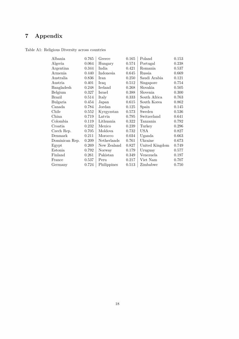
Islam. In this sample this applies to Iran, Iraq, Pakistan, Saudi Arabia, and Turkey. Table A1 in the

appendix presents the calculated index of religious diversity for those countries included in the empirical

analysis.

Since we have information on the religiosity score and religious diversity for three different points

of time, it would obviously be desirable to use panel estimation methods. However, religious diversity

is a very slow moving variable. Including country fixed effects will therefore eliminate every possibly

significant relationship between religiosity and religious diversity. Hence I will present the results of a

random effects estimation in the section on empirical results. However, the main insights will be drawn

from OLS regressions of the mean value of religiosity on the mean values of religious diversity, income, and

other control variables Xi, so that the estimated regressions are of the form:

religiosityi = α+ β · diversityi + γ · incomei + δ ·Xi + εi, (1)

where εi are robust standard errors.

In order to reduce the risk of reverse causality income should be used from a year before the first obser-

vation on religiosity, which is 1990. Only the Maddison (2010) online database offers income information

on the single former Soviet nations before the dissolution of the USSR. This data is available only for the

year 1973. I test the robustness of the results with income data from the Penn World Tables (Heston et

al., 2011). When income is used from 1973 the former Soviet and Yugoslav nations are dropped so that I

repeat the robustness test with all countries which is possible when income is taken from the year 1993.

7

Income is transformed into log terms because Paldam and Gundlach (2012) suggest that secularization is

a non-linear process.

I control for ethnic and linguistic diversity to take into account other possible cultural dimensions

apart from religious diversity. The information is taken from the afore mentioned paper by Alesina et al.

(2003) and is calculated equivalently to religious diversity. In addition I control for secondary education.

Information is taken from the World Bank Databank, based on the results from Barro and Lee (2010)

and measures the percentage of the population which completed secondary education. The Secularization

Hypothesis suggests a negative relationship with religiosity. As people become better informed, miraculous

explanations of scientific phenomena become insufficient or might be proven to be wrong. I include the

Polity IV score to test for possible effects of democratic institutions. Population size enters as another

control variable.

It might be argued that religious diversity is not exogenous to the level of religion. Therefore, I run an

instrumental variable regression to test the results gained by the OLS estimation. Fincher and Thornhill

(2008) propose that the disease environment can explain the distribution of religions across countries.

Harttgen and Opfinger (2012) show that these variables might be used as instruments for religious diversity.

In order to work as instrument in this analysis the disease environment must explain religious diversity but

must not be correlated with the level of religiosity. The first condition holds, as presented in Fincher and

Thornhill (2008). The authors argue that people separate themselves from groups with which they do not

share the same immunity pattern against contagious diseases. As a consequence separate cultures emerge

of which religion is an integral part. The more different immunity patterns existed, the more different

religions emerged as an evolutionary reaction which explains why there are different levels of religious

diversity today.

Fincher and Thornhill (2008) use the number of diseases and the number of pathogens as variables

in their study. The exclusion restriction requires that these variables do not affect religiosity through

another channel but religious diversity. It appears not immediately obvious how this should be the case.

The number of contagious diseases in a country which has led to an evolutionary emergence of different

cultures should not influence people’s perception of religiosity today. The questions used to calculate the

religiosity score ask about intrinsic involvement with the church and practiced religiosity. These should

be independent of the disease variables. One might argue that an increasing number of deaths due to a

disease might reduce faith due to disappointment or a feeling on unfairness. But however, this should lead

to a drop-out of religion which puts these people in the non-religious category. Or people form another

religion when they are disappointed with their old faith. Either way the reaction of religiosity should be

8

through religious diversity so that the exclusion restriction should hold unviolated.

Table 1: Summary statistics

Variable Mean Median Stan.Dev. Min MaxReligiosity score 57.43 56.20 19.66 15.18 89.99Religious Diversity 0.48 0.51 0.24 0.03 0.86Log Income 1973 8.49 8.61 0.90 6.21 9.81Secondary Education 37.53 37.40 18.34 1.40 80.13Ethnic Diversity 0.34 0.32 0.22 0.00 0.93Linguistic Diversity 0.30 0.22 0.26 0.00 0.92Polity Score 1973 -0.64 -7 8.17 -10 10Population in million 69.39 22.78 184.06 1.46 1200.90

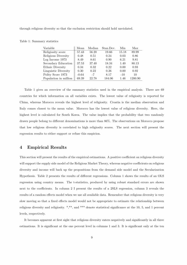
Table 1 gives an overview of the summary statistics used in the empirical analysis. There are 69

countries for which information on all variables exists. The lowest value of religiosity is reported for

China, whereas Morocco reveals the highest level of religiosity. Croatia is the median observation and

Italy comes closest to the mean value. Morocco has the lowest value of religious diversity. Here, the

highest level is calculated for South Korea. The value implies that the probability that two randomly

drawn people belong to different denominations is more than 86%. The observations on Morocco propose

that low religious diversity is correlated to high religiosity scores. The next section will present the

regression results to either support or refuse this suspicion.

4 Empirical Results

This section will present the results of the empirical estimations. A positive coefficient on religious diversity

will support the supply side model of the Religious Market Theory, whereas negative coefficients on religious

diversity and income will back up the propositions from the demand side model and the Secularization

Hypothesis. Table 2 presents the results of different regressions. Column 1 shows the results of an OLS

regression using country means. The t-statistics, produced by using robust standard errors are shown

next to the coefficients. In column 2 I present the results of a 2SLS regression, column 3 reveals the

results of a random effects model when we use all available data. Remember that religious diversity is very

slow moving so that a fixed effects model would not be appropriate to estimate the relationship between

religious diversity and religiosity. *,**, and *** denote statistical significance at the 10, 5, and 1 percent

levels, respectively.

It becomes apparent at first sight that religious diversity enters negatively and significantly in all three

estimations. It is significant at the one percent level in columns 1 and 3. It is significant only at the ten

9

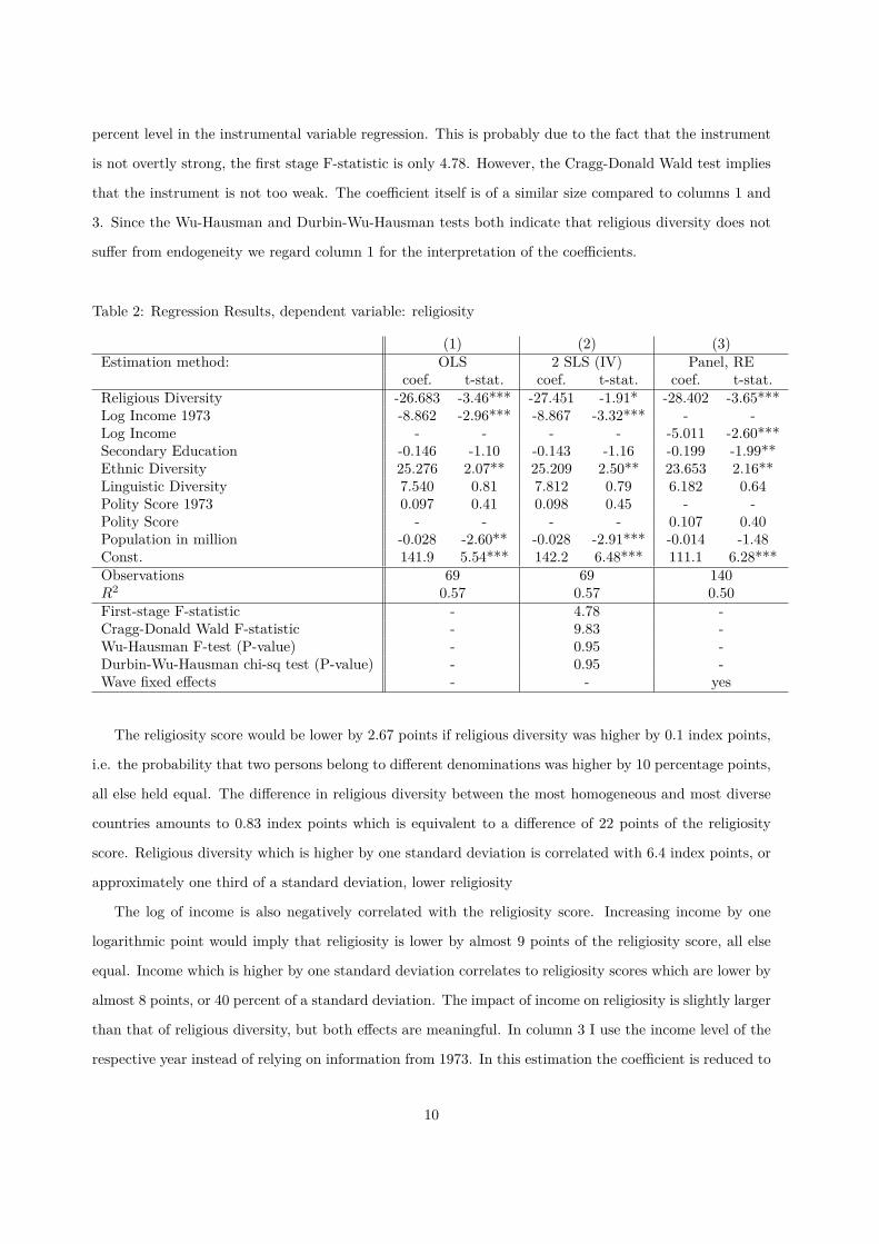
percent level in the instrumental variable regression. This is probably due to the fact that the instrument

is not overtly strong, the first stage F-statistic is only 4.78. However, the Cragg-Donald Wald test implies

that the instrument is not too weak. The coefficient itself is of a similar size compared to columns 1 and

3. Since the Wu-Hausman and Durbin-Wu-Hausman tests both indicate that religious diversity does not

suffer from endogeneity we regard column 1 for the interpretation of the coefficients.

Table 2: Regression Results, dependent variable: religiosity

(1) (2) (3)Estimation method: OLS 2 SLS (IV) Panel, RE

coef. t-stat. coef. t-stat. coef. t-stat.Religious Diversity -26.683 -3.46*** -27.451 -1.91* -28.402 -3.65***Log Income 1973 -8.862 -2.96*** -8.867 -3.32*** - -Log Income - - - - -5.011 -2.60***Secondary Education -0.146 -1.10 -0.143 -1.16 -0.199 -1.99**Ethnic Diversity 25.276 2.07** 25.209 2.50** 23.653 2.16**Linguistic Diversity 7.540 0.81 7.812 0.79 6.182 0.64Polity Score 1973 0.097 0.41 0.098 0.45 - -Polity Score - - - - 0.107 0.40Population in million -0.028 -2.60** -0.028 -2.91*** -0.014 -1.48Const. 141.9 5.54*** 142.2 6.48*** 111.1 6.28***Observations 69 69 140R2 0.57 0.57 0.50First-stage F-statistic - 4.78 -Cragg-Donald Wald F-statistic - 9.83 -Wu-Hausman F-test (P-value) - 0.95 -Durbin-Wu-Hausman chi-sq test (P-value) - 0.95 -Wave fixed effects - - yes

The religiosity score would be lower by 2.67 points if religious diversity was higher by 0.1 index points,

i.e. the probability that two persons belong to different denominations was higher by 10 percentage points,

all else held equal. The difference in religious diversity between the most homogeneous and most diverse

countries amounts to 0.83 index points which is equivalent to a difference of 22 points of the religiosity

score. Religious diversity which is higher by one standard deviation is correlated with 6.4 index points, or

approximately one third of a standard deviation, lower religiosity

The log of income is also negatively correlated with the religiosity score. Increasing income by one

logarithmic point would imply that religiosity is lower by almost 9 points of the religiosity score, all else

equal. Income which is higher by one standard deviation correlates to religiosity scores which are lower by

almost 8 points, or 40 percent of a standard deviation. The impact of income on religiosity is slightly larger

than that of religious diversity, but both effects are meaningful. In column 3 I use the income level of the

respective year instead of relying on information from 1973. In this estimation the coefficient is reduced to

10

5. But it still remains significant at the one percent level. The findings on religious diversity and income

both appear to favor the demand side model over the supply side model of the Religious Market Theory.

Table A2 in the appendix shows that the results hold when I use religious diversity from Alesina et al.

(2003) and income from the Penn World Tables (Heston et al., 2011).

The Secularization Hypothesis proposes that higher levels of education should lead to lower levels

of religiosity. In all three estimations the coefficient on secondary education is negative. However, this

finding is only statistically significant in the random effects estimation in column 3. Ethnic diversity enters

positively in the estimations. The size of the coefficient is similar to that of religious diversity but in the

opposite direction. That is not to mean that religious diversity is only significant because ethnic diversity

is included. Eliminating ethnic diversity from the list of control variables leaves the coefficient and the

significance level of religious diversity more or less unchanged1.

Population size enters negatively and significantly in the first two columns. However, the effect is fairly

small. Population which is larger by 1 million inhabitants is correlated to only 0.03 points lower religiosity

scores. Linguistic diversity and the Polity Score do not come close to statistical significance at conventional

levels.

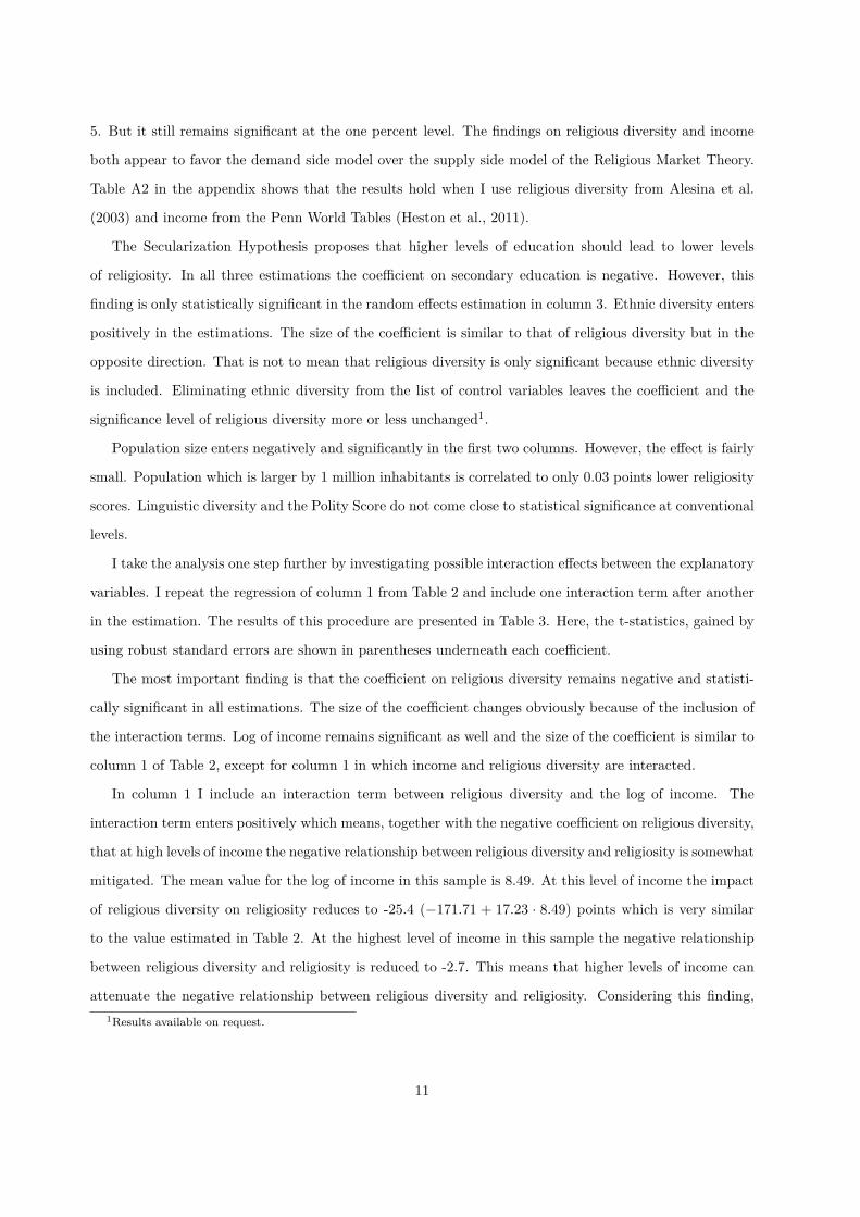
I take the analysis one step further by investigating possible interaction effects between the explanatory

variables. I repeat the regression of column 1 from Table 2 and include one interaction term after another

in the estimation. The results of this procedure are presented in Table 3. Here, the t-statistics, gained by

using robust standard errors are shown in parentheses underneath each coefficient.

The most important finding is that the coefficient on religious diversity remains negative and statisti-

cally significant in all estimations. The size of the coefficient changes obviously because of the inclusion of

the interaction terms. Log of income remains significant as well and the size of the coefficient is similar to

column 1 of Table 2, except for column 1 in which income and religious diversity are interacted.

In column 1 I include an interaction term between religious diversity and the log of income. The

interaction term enters positively which means, together with the negative coefficient on religious diversity,

that at high levels of income the negative relationship between religious diversity and religiosity is somewhat

mitigated. The mean value for the log of income in this sample is 8.49. At this level of income the impact

of religious diversity on religiosity reduces to -25.4 (−171.71 + 17.23 · 8.49) points which is very similar

to the value estimated in Table 2. At the highest level of income in this sample the negative relationship

between religious diversity and religiosity is reduced to -2.7. This means that higher levels of income can

attenuate the negative relationship between religious diversity and religiosity. Considering this finding,1Results available on request.

11

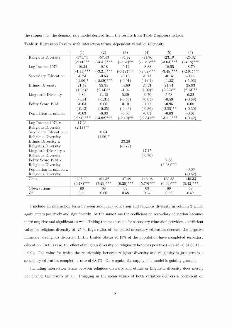
the support for the demand side model derived from the results from Table 2 appears to fade.

Table 3: Regression Results with interaction terms, dependent variable: religiosity

(1) (2) (3) (4) (5) (6)Religious Diversity -171.71 -57.43 -34.92 -31.76 -23.19 -25.32

(-2.60)** (-3.41)*** (-2.52)** (-2.79)*** (-3.03)*** (-3.18)***Log Income 1973 -16.34 -9.18 -9.12 -8.88 -10.55 -8.79

(-4.11)*** (-3.21)*** (-3.18)*** (-3.02)*** (-3.45)*** (-2.91)***Secondary Education -0.23 -0.63 -0.13 -0.13 -0.15 -0.14

(-1.90)* (-2.89)*** (-0.91) (-1.01) (-1.23) (-1.06)Ethnic Diversity 21.42 22.35 14.69 24.21 24.74 25.93

(1.98)* (2.14)** -1.04 (1.92)* (2.22)** (2.13)**Linguistic Diversity 9.89 11.15 5.89 -0.70 5.58 6.32

(-1.14) (-1.31) (-0.56) (-0.05) (-0.59) (-0.69)Polity Score 1973 -0.03 0.06 0.10 0.09 -0.95 0.08

(-0.13) (-0.25) (-0.43) (-0.36) (-2.55)** (-0.30)Population in million -0.03 -0.03 -0.03 -0.03 -0.03 -0.01

(-2.90)*** (-3.82)*** (-2.40)** (-2.34)** (-3.11)*** (-0.42)Log Income 1973 x 17.23Religious Diversity (2.17)**Secondary Education x 0.84Religious Diversity (1.96)*Ethnic Diversity x 23.26Religious Diversity (-0.72)Linguistic Diversity x 17.15Religious Diversity (-0.70)Polity Score 1973 x 2.38Religious Diversity (2.98)***Population in million x -0.03Religious Diversity (-0.52)Cons. 208.20 161.52 147.48 143.98 155.38 140.33

(6.78)*** (7.29)*** (6.20)*** (5.79)*** (6.09)*** (5.42)***Observations 69 69 69 69 69 69R2 0.60 0.60 0.58 0.57 0.62 0.57

I include an interaction term between secondary education and religious diversity in column 2 which

again enters positively and significantly. At the same time the coefficient on secondary education becomes

more negative and significant as well. Taking the mean value for secondary education provides a coefficient

value for religious diversity of -25.9. High ratios of completed secondary education decrease the negative

influence of religious diversity. In the United States 80.13% of the population have completed secondary

education. In this case, the effect of religious diversity on religiosity becomes positive (−57.43+0.84·80.13 =

+9.9). The value for which the relationship between religious diversity and religiosity is just zero is a

secondary education completion rate of 68.4%. Once again, the supply side model is gaining ground.

Including interaction terms between religious diversity and ethnic or linguistic diversity does merely

not change the results at all. Plugging in the mean values of both variables delivers a coefficient on

12

religious diversity of -27 and -26.6, respectively. The interaction term between the Polity Score and

religious diversity enters positively in column 5. The interpretation is similar to that on income and

education. In highly autocratic regimes with negative values of the Polity Score the negative relationship

between religious diversity and religiosity even becomes reinforced. In democratic countries the negative

relationship between religious diversity and religiosity can be overcome. Using the mean value of the Polity

score implies a coefficient on religious diversity of -24.7. For the most autocratic regimes the Polity Score

is -10. In this case the negative relationship between religious diversity and religiosity amounts to -47. The

Polity Score assigns a value of +10 to full democracies. Here, the relationship between religious diversity

and religiosity becomes marginally positive.

In the final column of Table 3 an interaction term between religious diversity and population is included.

It seems that this does not change the results much. However plugging in very high values for the population

size leads to large negative coefficients on religious diversity. A population size of 1.2 billion which is

observed for China in this sample implies a value of -61.3 for the relationship between religious diversity

and religiosity. It appears that in very large countries the negative relationship becomes stronger. However,

this appears to be only relevant for China and India. For the United States, the third largest country in

this sample the coefficient amounts to only -33.3 in column 6.

The results presented above deliver a mixed picture concerning the underlying models. The results

from Table 2 support the demand side model as religious diversity and religiosity appear to be negatively

correlated. However, including interaction terms reveals that income, education, and democracy can

mitigate this effect. For the most developed countries the relationship can even turn positive which

favors the supply side model. Nevertheless, the results on income appear to support the Secularization

Hypothesis.

5 Discussion

This paper is supposed to reassess the relationship between religious diversity and religiosity and thereby

finding support for either the demand side or supply side model. Bar-El et al. (2013) propose that both

mechanisms might be at work at the same time but that one dominates the other. However, the ranking

of mechanisms may change over time.

The results gained above leave room for a similar explanation. The baseline results from Table 2

propose that there is a negative linear relationship between religious diversity and the level of religiosity

which supports the demand side model of the Secularization Hypothesis. However, the results on the

interaction terms which are presented in Table 3 reveal that this straight-forward solution would be overtly

13

simple. High levels of income, secondary education, and democracy can turn the coefficient on religious

diversity from negative to positive which in turn supports the supply side model of the Religious Market

Theory.

It appears that different mechanisms are in force at different stages of economic development. The

structure of the market for religion does not seem to play an important role in less developed countries.

Religion is more prominent in these societies for everyday decision making. If the trust in the respective

belief is shaken due to the uprising of new churches, people will reduce their overall level of religiosity. This

reaction looses power if religion itself is not as important as it has been before. This is the case in the more

developed nations. As Hirschle (2011) shows, religiosity is substituted for other activities when income

rises. Due to higher education religious myths are no longer necessary to explain certain experiences but

there are scientific explanations for most of nature’s phenomena. Consequently, people may become more

liberal towards switching denominations and looking for a faith which fits best their values and beliefs.

Another explanation may be that people concentrate more on the maximization of their own utility. This

is maximized when they switch to another belief. It follows that the consumers choose the denomination

which offers the religious good with the highest quality. According to the Religious Market Theory, the

quality increases when more churches compete for believers and therefore we can explain why there might

be a positive relationship between religious diversity and religiosity in the most developed countries.

As Bar-El et al. (2013) propose, both mechanisms seem to be present at the same time. But one

force always dominates the other. The demand side forces are stronger at low stages of economic devel-

opment. People who doubt the correctness of their faith reduce their religious involvement. As economic

development proceeds the supply side forces become stronger. Believers feel attracted to churches whose

preachings fit their own preferences. They become more liberal to switching religions, instead of reducing

religious involvement, which is probably due to the fact that religion itself is not as important anymore in

the developed countries.

The results on democracy give further interesting insights. Diversity has a negative effect on religiosity

in highly autocratic regimes. Put the other way, the finding proposes that religiosity is higher and probably

more important if one sticks to the majority faith, which might itself be chosen by the autocratic leader.

This together with the oppression of other religions may make it socially advantageous to be highly

involved in the chosen religion. On the other hand, people are free to choose their religion in democratic

countries. This makes switching denominations easier and more attractive. Once people find the faith

which maximizes their utility, they increase their overall religious involvement.

The results on income provide evidence for the existence and validity of the Secularization Hypothesis.

14

It appears that ongoing economic development decreases the importance of religiosity for people’s lives.

This might be the reason for why the supply side forces dominate in the most developed societies once

Secularization has occurred.

Using the above argument can also explain why Iannaccone (1991) finds strong support for his Religious

Market Theory. He explains that he uses data on ”17 Western industrialized countries”. The supply side

effect should have a strong influence on those because Secularization has already happened. In fact,

running the regression from Table 2 column 1 with the countries included in Iannaccone’s (1991) study

reveals a coefficient on religious diversity of only -4, which is statistically not significantly different from

zero. Although the supply side model still would not be endorsed in this case, neither would be the

demand side model. It appears that the demand side model dominates for the less developed countries

before Secularization takes place. In the course of Secularization, whose existence is proven by the results

on income, the importance of religiosity decreases. In the secularized, developed societies the supply side

forces take over and competition between churches increases the level of religiosity. This hypothesis of

supply side factors coming into force after Secularization should be evaluated further in future research.

6 Conclusion

The Religious Market Theory proposes a supply side model for the market of religion. Basic microeconomic

modeling implies that monopoly churches reduce effort in producing the religion good in order to increase

profits. However, consumers will demand less of the inferior goods. Churches in competitive markets

provide goods of higher quality for which demand is higher. It follows that higher religious diversity

should lead to higher levels of religiosity.

In contrast, the demand side model which originates from the Secularization Hypothesis proposes that

people reduce the ties to religiosity when they start to doubt the correctness of their faith. Hence, the

existence of many different churches, i.e. high religious diversity will lead to low levels of religiosity.

This paper reassesses the relationship between religious diversity and religiosity. For this purpose

I rely on a new measure for religiosity from Paldam and Gundlach (2012) which should produce more

accurate results than earlier studies which rely on church attendance rates. The results indicate that

both models might be in force at the same time, but that one effect dominates the other depending on

the level of economic development. At low stages of economic development we find that the demand side

model better describes people’s behavior, as there is a negative relationship between religious diversity and

religiosity. However, high levels of income, education, and democracy can alleviate this effect, so that the

relationship turns to positive in the most developed societies. The supply side model seems to dominate

15

once Secularization has occurred.

References

Alesina, A., Devleeschauwer, A., Easterly, W., Kurlat, S., Wacziarg, R. (2003), ’Fractionalization’, Journal

of Economic Growth 8,155-194.

Bar-El, R., Garcia-Munoz, T., Neuman, S., Tobol, Y. (2012), ’The evolution of secularization: cultural

transmission, religion and fertility - theory, simulations and evidence’, Journal of Population

Economics doi: 10.1007/s00148-011-0401-9.

Barrett, D.B., Kurian, G.T., Johnson, T.M. (2001), World Christian Encyclopedia, Oxford University

Press, Oxford.

Barro, R.J., Lee, J.W. (2010), ’A New Data Set of Educational Attainment in the World, 1950-2010’,

NBER Working Paper 15902

Barro, R.J., McCleary, R. (2002), ’Religion and Political Economy in an International Panel’, Journal for

the Scientific Study of Religion 45,149-175.

Blau, J.R., Redding, K., Land, K.C. (1993), ’Ethnocultural Cleavages and the Growth of Church

Membership in the United States, 1860-1930’, Sociological Forum 8,609-637.

Breault, K.D. (1989), ’New Evidence on Religious Pluralism, Urbanism, and Religious Participation’,

American Sociologiacal Review 54,1048-1053.

Bruce, S. (2000), ’The Supply-Side Model of Religion: The Nordic and Baltic States’, Journal for the

Scientific Study of Religion 39,32-46.

Casanova, J. (1994), Public religions in the modern world. University of Chicago Press, Chicago.

Chaves, M. (1994), ’Secularization as declining religious authority’, Social Forces 72,749-774.

Chaves, M., Gorski, P.S. (2001), ’Religious Pluralism and Religious Participation’, Annual Review

Sociology 27,261-281.

Fincher, C.L., Thornhill, R. (2008), ’Assortative sociality, limited dispersal, infectious disease and the

genesis of the global pattern of religious diversity’, Proceedings of the Royal Society B: Biological

Sciences.

Finke, R., Stark, R. (1988), ’Religious Economies and Sacred Canopies: Religious Mobilization in

American Cities, 1906’, American Sociological Review 53,41-49.

Franck, R., Iannaccone, L.R. (2009), ’Why did religiosity decrease in the Western World during the

twentieth century?’, Bar-Ilan University Discussion Paper.

Gruber, J. (2005), ’Religious Market Structure, Religious Participation, and Outcomes: Is Religion Good

16

For You?’ NBER Working Paper 11377.

Glock, C.Y., Stark, R. (1965), Religion and Society in Tension. Rand McNally & Company, Chicago.

Hanson, G.H., Xiang, C. (2011), ’Exporting Christianity: Governance and Doctrine in the Globalization

of US Denominations’, NBER Working Paper 16964.

Harttgen, K., Opfinger, M. (2012), ’National Identity and Religious Diversity’, Research Papers in

Economics, University Trier, 07/12

Heston, A., Summers, R., Aten, B. (2011), ’Penn World Table Version 7.0’, Center for International

Comparisons of Production, Income and Prices at the University of Pennsylvania, June 2011.

Hirschle, J. (2011), ’The affluent society and its religious consequences: an empirical investigation of 20

European countries’, Socio-Economic Review 9,261-285.

Iannaccone, L.R. (1991), ’The Consequences of Religious Market Structure’, Rationality and Society

3,156-177.

Inglehart, R., Baker, W.E. (2000), ’Modernization, Cultural Change, and the Persistence of Traditional

Values’, American Sociological Review 65,19-51.

Maddison, A. (2010), ’Statistics on World Population, GDP and Per Capita GDP, 1-2008 AD’.

Martin, D. (1978), A General theory of Secularization. Harper & Row, New York.

McCleary, R., Barro, R.J. (2006), ’Religion and Economy’, Journal of Economic Perspectives 20,49-72.

Olson, D.V.A. (1999), ’Religious Pluralism and US Church Membership: A Reassessment’, Sociology of

Religion 60,149-173.

Paldam, M., Gundlach, E. (2012), ’The religious transition: A long-run perspective’, Public Choice, doi:

10.1007/s11127-012-9934-z.

Sherkat, D.E. (1991), ’Leaving the Faith: Testing Theories of Religious Switching Using Survival Models’,

Social Science Research 20,171-187.

Tschannen, O. (1994), ’Sociological controversies in perspective’, Review of Religious Research 36,70-86.

Voas, D., Crockett, A., Olson, D.V.A. (2002), ’Religious Pluralism and Participation: Why Previous

Research Is Wrong’, American Sociological Review 67,212-230.

Yamane, D. (1997), ’Secularization on trial: In defense of a neosecularization paradigm’, Journal for the

Scientific Study of Religion 36,109-122.

17

7 Appendix

Table A1: Religious Diversity across countries

Albania 0.765 Greece 0.165 Poland 0.153Algeria 0.064 Hungary 0.574 Portugal 0.238Argentina 0.344 India 0.421 Romania 0.537Armenia 0.440 Indonesia 0.645 Russia 0.669Australia 0.836 Iran 0.250 Saudi Arabia 0.121Austria 0.401 Iraq 0.512 Singapore 0.754Bangladesh 0.248 Ireland 0.268 Slovakia 0.505Belgium 0.327 Israel 0.388 Slovenia 0.300Brazil 0.514 Italy 0.333 South Africa 0.763Bulgaria 0.454 Japan 0.615 South Korea 0.862Canada 0.784 Jordan 0.125 Spain 0.145Chile 0.552 Kyrgyzstan 0.573 Sweden 0.536China 0.719 Latvia 0.795 Switzerland 0.641Colombia 0.119 Lithuania 0.322 Tanzania 0.792Croatia 0.232 Mexico 0.239 Turkey 0.296Czech Rep. 0.705 Moldova 0.732 USA 0.827Denmark 0.211 Morocco 0.034 Uganda 0.663Dominican Rep. 0.209 Netherlands 0.761 Ukraine 0.673Egypt 0.269 New Zealand 0.827 United Kingdom 0.749Estonia 0.792 Norway 0.179 Uruguay 0.577Finland 0.261 Pakistan 0.349 Venezuela 0.197France 0.537 Peru 0.217 Viet Nam 0.707Germany 0.724 Philippines 0.513 Zimbabwe 0.750

18

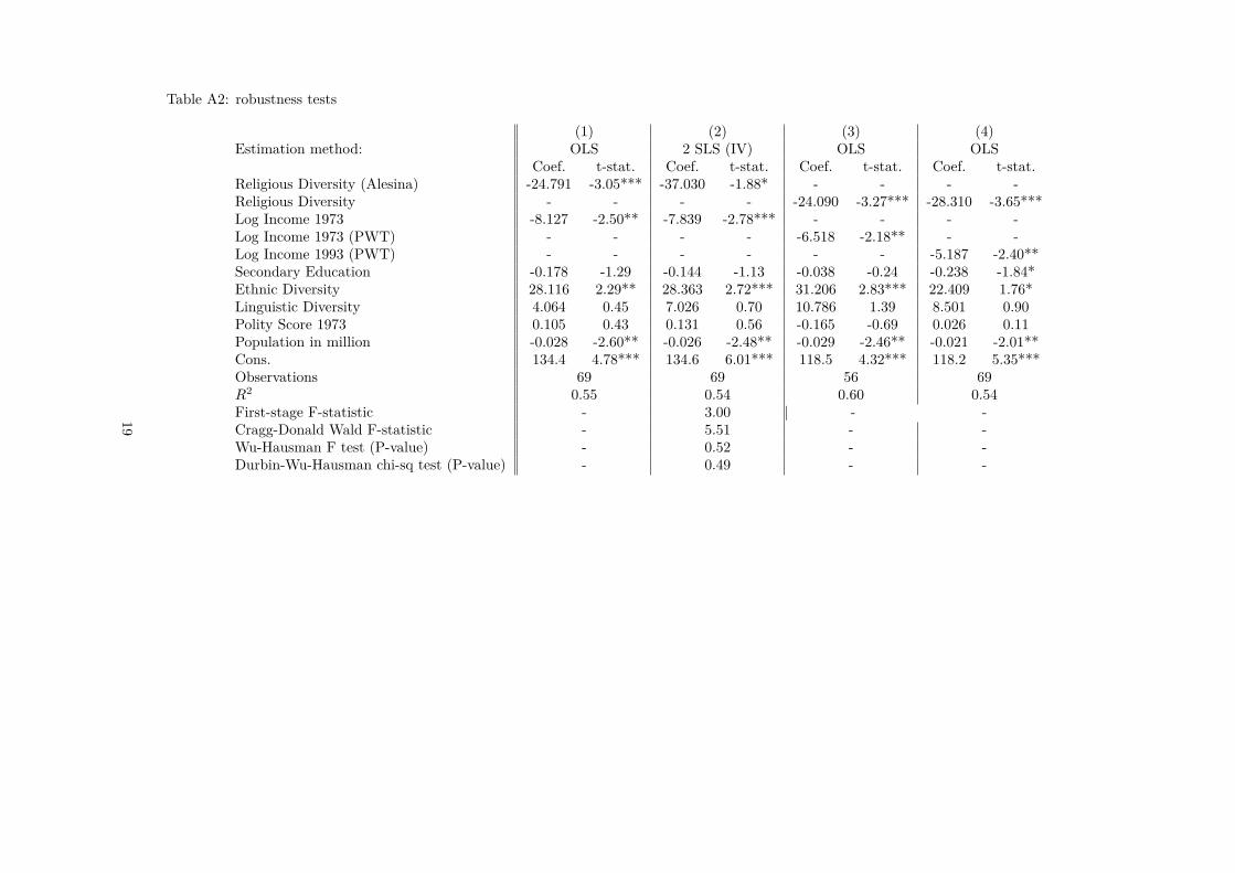
Table A2: robustness tests

(1) (2) (3) (4)Estimation method: OLS 2 SLS (IV) OLS OLS

Coef. t-stat. Coef. t-stat. Coef. t-stat. Coef. t-stat.Religious Diversity (Alesina) -24.791 -3.05*** -37.030 -1.88* - - - -Religious Diversity - - - - -24.090 -3.27*** -28.310 -3.65***Log Income 1973 -8.127 -2.50** -7.839 -2.78*** - - - -Log Income 1973 (PWT) - - - - -6.518 -2.18** - -Log Income 1993 (PWT) - - - - - - -5.187 -2.40**Secondary Education -0.178 -1.29 -0.144 -1.13 -0.038 -0.24 -0.238 -1.84*Ethnic Diversity 28.116 2.29** 28.363 2.72*** 31.206 2.83*** 22.409 1.76*Linguistic Diversity 4.064 0.45 7.026 0.70 10.786 1.39 8.501 0.90Polity Score 1973 0.105 0.43 0.131 0.56 -0.165 -0.69 0.026 0.11Population in million -0.028 -2.60** -0.026 -2.48** -0.029 -2.46** -0.021 -2.01**Cons. 134.4 4.78*** 134.6 6.01*** 118.5 4.32*** 118.2 5.35***Observations 69 69 56 69R2 0.55 0.54 0.60 0.54First-stage F-statistic - 3.00 | - -Cragg-Donald Wald F-statistic - 5.51 - -Wu-Hausman F test (P-value) - 0.52 - -Durbin-Wu-Hausman chi-sq test (P-value) - 0.49 - -

19