Mutual Funds and Mispriced Stocks

Mutual Funds and Mispriced Stocks*

By Doron Avramov, Si Cheng, and Allaudeen Hameed

January 25, 2019

Abstract

We propose a new measure of fund investment skill, Active Fund Overpricing (AFO), encapsulating

the fund’s active share of investments, the direction of fund active bets with regard to mispriced stocks,

and the dispersion of mispriced stocks in the fund’s investment opportunity set. We find that fund

activeness is not sufficient for outperformance: high (low) AFO funds take active bets on the wrong

(right) side of stock mispricing achieve inferior (superior) fund performance. However, high AFO funds

receive higher flows during periods of high investor sentiment, when performance-flow relation

becomes weaker.

Keywords: Mutual funds; Managerial Skills; Mispricing

__________________________________________

* Doron Avramov (email: [email protected]) is from IDC Herzliya; Si Cheng (email: [email protected]) is from

Chinese University of Hong Kong, and Allaudeen Hameed (email: [email protected]) is from National University of

Singapore. We thank two anonymous referees, the associate editor, Yakov Amihud, Scott Cederburg, Alexander Chinco,

Martin Cremers, Karl Diether (editor), Joni Kokkonen, Lin Peng, Jianfeng Shen, Ashley Wang, Hong Zhang, and seminar

participants at INSEAD, Queen’s University Belfast, Shanghai Advanced Institute of Finance (SAIF), Tel Aviv University,

The Chinese University of Hong Kong, Tsinghua University, University College Dublin, University of New South Wales,

University of Sydney, University of Technology Sydney, 2015 Luxembourg Asset Management Summit, 2015 Tel Aviv

Finance Conference, 2016 China International Conference on Finance, and 2016 FMA European Conference for helpful

comments. Hameed gratefully acknowledges the financial support from NUS Academic Research Grant.

mailto:[email protected]



Mutual Funds and Mispriced Stocks

Abstract

We propose a new measure of fund investment skill, Active Fund Overpricing (AFO), encapsulating

the fund’s active share of investments, the direction of fund active bets with regard to mispriced stocks,

and the dispersion of mispriced stocks in the fund’s investment opportunity set. We find that fund

activeness is not sufficient for outperformance: high (low) AFO funds that take active bets on the wrong

(right) side of stock mispricing achieve inferior (superior) fund performance. However, high AFO funds

receive higher flows during periods of high investor sentiment, when performance-flow relation

becomes weaker.

Keywords: Mutual funds; Managerial Skills; Mispricing

1

1. Introduction

Recent statistics from the Investment Company Institute show that the total net assets managed by

3,193 U.S. domestic equity mutual funds exceed 7.4 trillion dollar as of April 2018. Funds aim to create

value for their investors through their skills in stock picking and market timing (e.g., Fama (1972), and

Daniel, Grinblatt, Titman, and Wermers (DGTW) (1997)). As mutual funds typically undertake long-

only positions, stock picking skills involve identifying mispriced stocks and actively overweighting

undervalued assets and underweighting (or avoiding) overpriced assets. There is also a large body of

evidence in support of mispricing identified by market anomalies. For example, Stambaugh, Yu, and

Yuan (2012, 2015) and Avramov, Chordia, Jostova, and Philipov (2013) show that many market

anomalies extract their profitability from selling short overpriced stocks. Their findings are consistent

with impediments to arbitrage such as short-sale constraints giving rise to stock prices that reflect the

views of the more optimistic investors in the presence of heterogeneous beliefs about fundamental

values (Miller (1977)). In the context of mutual funds, Akbas, Armstrong, Sorescu, and Subrahmanyam

(2015) and Edelen, Ince, and Kadlec (2016) show that funds do not exploit predictability in the cross

section of equity returns. Perhaps surprisingly, the mutual funds, in aggregate, tend to buy the stocks

belonging to the short-leg of anomalies and appear to exacerbate cross-sectional mispricing.1

In this paper, we develop a new measure of fund investment skill based on the active positions

undertaken by funds with regard to mispriced stocks. To do this, we start with the identification of

relatively overpriced stocks using the eleven well-known stock market anomalies in Stambaugh, Yu,

and Yuan (2012). The overpricing measure is based on the notion that anomalies reflect mispricing and

averaging across many anomalies identifies mispriced stocks. We propose an active fund overpricing

(AFO) measure as the active deviation of mutual fund investment in overpriced stocks relative to the

investment weights implied by their benchmark portfolio. In other words, AFO is the difference between

the fund level investment-value-weighted average of stock-level overpricing and the average

overpricing implied by the stocks in the fund’s benchmark portfolio. To be precise, 𝐴𝐹𝑂𝑓,𝑞 for fund f

1 There are some, albeit limited, evidence that mutual funds profit from anomalies. For example, the top ten percent of mutual

funds that actively follow the accrual strategy earn positive alphas (Ali, Chen, Yao, and Yu (2008)). Furthermore, others show

that anomalies such as momentum survive reasonable transaction costs incurred by institutions (Korajczyk and Sadka (2004)).

2

at time q describes the covariance between fund f’s active portfolio weights (i.e., fund f’s active

deviation from benchmark implied weights) and overpricing of the stocks in the fund’s investment

universe. We hypothesize that high (low) AFO funds are associated with low (high) stock picking skills

as they actively overweight (underweight) overpriced stocks and are expected to earn low (high) future

returns as the mispricing in stocks get corrected in the next period.

We construct quarterly AFO for the actively managed U.S. equity funds that meet our data

requirements for the period 1981 to 2010. We find that higher AFO funds display higher total net assets,

higher expense ratio, higher turnover, and hold less liquid stocks. In addition, the cross-sectional

difference in the active exposure of mutual funds to mispriced stocks is highly persistent: the propensity

of a fund to actively hold overpriced stocks in a quarter continues into subsequent quarters. For example,

more than half of the high (low) AFO funds remain in the top (bottom) decile after one year.

We focus our investigation on the relation between AFO and future fund performance. We find that

the cross-sectional variation in the risk-adjusted future performance of active mutual funds is

significantly related to the fund’s AFO. Funds in the top decile of AFO-sorted portfolios underperform

those in the bottom decile by 2.27% in benchmark-adjusted return and by 1.8% in Fama-French-Carhart

(FFC) four-factor adjusted return per annum. The performance gap widens considerably during episodes

of high market sentiment: the highest AFO funds underperform the lowest AFO funds by 4.86% in

benchmark-adjusted return and by 2.56% in FFC-adjusted return per annum.

The cross-sectional negative relation between AFO and future fund returns is robust. Our main

finding remains intact when we control for fund-specific characteristics (such as fund size and fund

expenses) in panel and Fama-MacBeth regressions. We also consider if there are time-series variations

in the predictive relation between the fund’s AFO and future performance. We do this by incorporating

fund fixed effects in panel regressions of fund performance (i.e., fund returns adjusted by various

performance models) on past AFO and other fund characteristics. Again, we find significant predictable

time-series variations in fund performance linked to AFO: a one standard deviation higher AFO predicts

a reduction of benchmark-adjusted (annualized) return of 1.03% for the fund. The cross-sectional and

time-series variations in the AFO-fund performance relation we document are qualitatively similar

when we use difference fund performance metrics.

3

To better understand the sources of fund skill, AFO is decomposed into the product of three

components: (i) the correlation between the fund’s active investment weights (i.e., relative to the fund’s

benchmark weights) and stock overpricing (denoted as COROP), (ii) standard deviation of the fund’s

active investment weights (denoted as STDAS), and (iii) standard deviation of stock overpricing

(denoted as STDOP). High values of COROP reflects the fund’s lack of skill in active portfolio

management, as a positive or high correlation indicates the fund overweighting overpriced stocks

relative to the benchmark. The second component, STDAS, reflects active share in the spirit of Cremers

and Petajisto (2009) and Petajisto (2013). When a fund has a high STDAS, it implies that the fund takes

active positions in stocks by deviating from the benchmark portfolio weights. The final component,

STDOP, defines the potential investment opportunity set encountered by the fund in terms of dispersion

in stock level overpricing. In sum, AFO integrates three elements into one unified metric: the fund’s

active stock picking skill, the degree of activeness of the fund, and the potential investment

opportunities among mispriced stocks.

When we break down AFO into the above three components, the correlation between active fund

investment weights and stock overpricing (COROP) is the strongest and most consistent predictor of

fund performance. While high STDAS funds (i.e., funds with high active share) appear to be associated

positively with future performance, the association is weak. Specifically, controlling for COROP,

activeness of the fund does not contain substantial predictive content for future fund returns. Finally,

we find that the stock level overpricing represented by STDOP plays a minor role in predicting fund

returns. Consequently, the source of return predictability of AFO comes from the ability of funds to

deviate from their benchmark weights in the direction against overpricing, beyond merely being active.

Our findings make a significant contribution to the debate in the literature on the relation between

active share (which is related to our STDAS component) and fund performance. For example, Frazzini,

Friedman, and Pomorski (2016) argue that active share correlates with the returns on the fund’s

benchmark portfolio reported in Cremers and Petajisto (2009) and does not predict actual fund returns.

AFO provides an improvement to the active share measure presented in Cremers and Petajisto (2009)

by better isolating the fund manager’s active management skill. Our findings highlight the intuition that

high active share (or STDAS) funds may earn high or low future returns depending on whether the fund

4

is underweighting (negative COROP) or overweighting (positive COROP) overpriced stocks. In other

words, fund activeness is not a sufficient measure of skill, as fund managers could deviate from

benchmark in the wrong direction by overweighting overpriced stocks. Hence, our AFO based results

emphasize the importance of funds being active in the right direction. Our AFO measure is also closely

related to the Active Fundamental Performance proposed by Jiang and Zheng (2018). Active

Fundamental Performance identifies skilled managers if they overweight stocks with high cumulative

abnormal returns surrounding the quarterly earnings announcement, while our AFO measure identifies

skilled managers if they overweight underpriced stocks.

Our findings also emphasize the joint effects of stock mispricing and investor sentiment on fund

performance and complement the stock-level findings in Stambaugh, Yu, and Yuan (2012). We provide

statistically and economically significant evidence that AFO is inversely related to fund performance

after controlling for other predictors of fund performance including tracking error (Wermers (2003),

Cremers and Petajisto (2009)), industry concentration index (Kacperczyk, Sialm, and Zheng (2005)),

active share (Cremers and Petajisto (2009), Petajisto (2013)), and R-squared (Amihud and Goyenko

(2013)).2 The negative AFO-fund performance relation is primarily driven by the active stock picking

skill of the fund manager, which is enhanced when sentiment is high.

An alternative interpretation of the AFO-fund performance relation is that there are mispricing

factors excluded from the risk-adjustment specification commonly used in the literature. If so, alpha

variation across funds reflects different exposures of fund returns to mispricing factors with high AFO

funds exhibiting lower exposures. Empirical support for mispricing factors is provided by Kogan and

Tian (2015) and Stambaugh and Yuan (2017). They show that characteristics-based anomalies share

common return co-movement and factors created from anomalies capture much of the cross-sectional

variation in average stock returns. Notice also that Kozak, Nagel, and Santosh (2018) imply that alphas

due to mispricing related to investor sentiment are indistinguishable from exposures to mispricing

factors. Our empirical evidence indeed shows that mispricing factors play an important role in capturing

2 Our evidence on the cross-sectional relation between fund overpricing and performance adds to Pástor, Stambaugh, and

Taylor (2017)’s findings on the relation between time variation in fund trading activity and manager skill. They find that funds

trade more when investor sentiment is high, consistent with funds trading heavily when stocks are more mispriced.

5

the cross-sectional fund returns based on AFO. However, we find (albeit weak) relation between AFO

and mispricing factor-adjusted fund performance during periods of high sentiment. An interesting

implication of our findings is that the four-factor model (market, size, and two mispricing factors)

proposed in Stambaugh and Yuan (2017) provides an additional metric to evaluate the performance of

mutual fund managers, as actively managed mutual funds often bet on mispriced stocks.

Miller’s (1977) basic assertion implies that overpriced funds are likely to be held by optimistic

investors. In high sentiment periods, overpriced funds could attract additional flows as optimistic

investors, buoyed by positive market sentiment, pour more money into such funds. On the other hand,

prior studies have also shown that fund flows are influenced by other fund characteristics, particularly

past fund returns, as investors are known to chase past performance (e.g., Chevalier and Ellison (1997))

and overpriced funds are typically recent underperformers. Interestingly, we find a significant positive

relation between AFO and future flows, particularly during periods of high investor sentiment. The

increase in flows to high AFO funds is explained by considerably weaker sensitivity of fund flows to

past performance when sentiment is high. Our findings imply that during high sentiment periods,

optimistic mutual fund investors are less sensitive to past fund performance, and are more likely to

invest in active funds. As the results are robust to benchmark-adjusted fund flows, the positive AFO-

fund flow relationship is not driven by investor demand in a particular style or benchmark. Hence,

despite poor stock picking skills, high AFO (active) funds are able to attract flows, especially during

high sentiment periods.

The rest of the paper is organized as follows. Section 2 describes the data and the construction of

the variables of interest. Section 3 presents some stylized patterns of AFO. Section 4 studies the

implications of active fund overpricing for future performance. Section 5 relates active fund overpricing

to investor response in terms of flows. Section 6 concludes.

2. Variable Construction and Data Description

2.1. Active Fund Overpricing (AFO) Measure

We measure the degree of mutual fund level active overpricing by aggregating the overpricing of

stocks held by the fund in excess of the overpricing implied by the stocks in the fund’s benchmark

6

portfolio. Following Stambaugh, Yu, and Yuan (2012), we construct stock-level overpricing based on

eleven anomalies that survive exposures to the three factors of Fama and French (1993). Each anomaly

reflects mispriced stocks and by combining the eleven anomalies, we obtain mispricing information

that is common across all these anomalies (Stambaugh, Yu, and Yuan (2015)). The eleven anomalies

consist of failure probability (e.g., Campbell, Hilscher, and Szilagyi (2008), Chen, Novy-Marx, and

Zhang (2011)), O-Score (Ohlson (1980), Chen, Novy-Marx, and Zhang (2011)), net stock issuance

(Ritter (1991), Loughran and Ritter (1995)), composite equity issuance (Daniel and Titman (2006)),

total accruals (Sloan (1996)), net operating assets (Hirshleifer, Hou, Teoh, and Zhang (2004)),

momentum (Jegadeesh and Titman (1993)), gross profitability (Novy-Marx (2013)), asset growth

(Cooper, Gulen, and Schill (2008)), return on assets (Fama and French (2006)), and abnormal capital

investment (Titman, Wei, and Xie (2004)). We simply adopt the set of anomalies in Stambaugh, Yu,

and Yuan (2012) to avoid any perceived bias in the selection of anomalies.

Stock-level overpricing is constructed as follows. For each anomaly, we rank the stocks in each

quarter with the highest rank indicating the most overpriced stock. Ranks are normalized to follow a [0,

1] uniform distribution. For example, more overpriced stocks, or stocks with higher failure probability,

higher O-Score, higher net stock issuance, higher composite equity issuance, higher total accruals,

higher net operating assets, lower past six-month returns, lower gross profitability, higher asset growth,

lower return on assets, and higher abnormal capital investment receive higher ranks (closer to 1). A

stock’s composite rank is the equal-weighted average of its ranks across all eleven anomalies, and we

denote this stock-level overpricing measure for stock 𝑖 in quarter 𝑞 as 𝑂𝑖,𝑞.

We proceed to construct fund-level active overpricing as the investment value-weighted average of

stock-level overpricing minus the average overpricing implied by the stocks in the fund’s benchmark

portfolio. In particular, using stocks in fund f’s most recently reported portfolio holdings in quarter q,

we define the active fund overpricing measure (𝐴𝐹𝑂𝑓,𝑞) as follows:

𝐴𝐹𝑂𝑓,𝑞 = ∑ (𝑤𝑖,𝑓,𝑞 − 𝑤𝑖,𝑓,𝑞𝑏 )𝑂𝑖,𝑞𝑖 , (1)

7

where 𝑤𝑖,𝑓,𝑞 is the investment weight of stock i in fund f in quarter q and 𝑤𝑖,𝑓,𝑞𝑏 is the investment weight

of stock i in fund f’s benchmark portfolio in the same quarter.3 Thus, our fund-level overpricing measure

is related to the activeness of the fund’s investment in mispriced stocks. A high 𝐴𝐹𝑂𝑓,𝑞 implies that

fund f actively overweights (underweights) overpriced (underpriced) stocks relative to the benchmark

portfolio weights. Similarly, funds that invest less than their benchmarks in overpriced stocks display

low 𝐴𝐹𝑂𝑓,𝑞. To better understand the active fund overpricing measure, 𝐴𝐹𝑂𝑓,𝑞 is decomposed into the

product of three components:

𝐴𝐹𝑂𝑓,𝑞 = 𝑁𝑓,𝑞𝐶𝑜𝑣(𝑤𝑖,𝑓,𝑞 − 𝑤𝑖,𝑓,𝑞𝑏 , 𝑂𝑖,𝑞) = 𝜌(𝑤𝑖,𝑓,𝑞 − 𝑤𝑖,𝑓,𝑞

𝑏 , 𝑂𝑖,𝑞)𝑁𝑓,𝑞𝜎(𝑤𝑖,𝑓,𝑞 − 𝑤𝑖,𝑓,𝑞𝑏 )𝜎(𝑂𝑖,𝑞), (2)

where 𝑁𝑓,𝑞 is the number of stocks in fund f’s investment universe, including the stocks held by the

fund and those in the fund’s benchmark portfolio. All other variables are defined in Equation (1). The

decomposition of the AFO measure is similar in spirit to the separation of the Active Fundamental

Performance metric into multiple parts in Jiang and Zheng (2018). In particular, the first component in

Equation (2), 𝜌(𝑤𝑖,𝑓,𝑞 − 𝑤𝑖,𝑓,𝑞𝑏 , 𝑂𝑖,𝑞) , measures the correlation between the benchmark-adjusted

investment weight of stock i in fund f and overpricing of stock i, which we label as 𝐶𝑂𝑅𝑂𝑃𝑓,𝑞 . A

positive 𝐶𝑂𝑅𝑂𝑃𝑓,𝑞 means that the deviation of fund f’s investment relative to the fund’s benchmark is

positively correlated with the level of stock overpricing. In other words, positive 𝐶𝑂𝑅𝑂𝑃𝑓,𝑞 implies that

fund f actively deviates from benchmark portfolio weights by tilting its holdings towards more

overpriced stocks and away from less overpriced stocks. A negative 𝐶𝑂𝑅𝑂𝑃𝑓,𝑞 is obtained when a fund

overweights less overpriced stocks relative to the benchmark weights. Thus, a positive (negative)

𝐶𝑂𝑅𝑂𝑃𝑓,𝑞 indicates poor (good) managerial skill with respect to picking mispriced stocks as defined

by the anomalies. Hence, the 𝐶𝑂𝑅𝑂𝑃𝑓,𝑞 component of 𝐴𝐹𝑂𝑓,𝑞 proxies for the active stock picking skill

of the fund manager.

The second component in Equation (2), 𝑁𝑓,𝑞𝜎(𝑤𝑖,𝑓,𝑞 − 𝑤𝑖,𝑓,𝑞𝑏 ), measures the standard deviation of

benchmark-adjusted investment weight, and is labelled as 𝑆𝑇𝐷𝐴𝑆𝑓,𝑞. This is similar to the active share

3 As most anomalies are formed annually and do not vary within a quarter, we also construct the overpricing measure at the

annual frequency. Our findings are similar across these sampling frequencies.

8

proxy in Cremers and Petajisto (2009) and Petajisto (2013), which is defined as the absolute difference

in investment weights of fund f relative to its benchmark weights. A higher 𝑆𝑇𝐷𝐴𝑆𝑓,𝑞 stands for greater

deviation from the corresponding benchmark weights and hence more active investment. Notice that

the product of the first two components (i.e., 𝐶𝑂𝑅𝑂𝑃𝑓,𝑞 and 𝑆𝑇𝐷𝐴𝑆𝑓,𝑞) indicates that high active share

could generate positive performance only if the activeness is in the right direction, i.e., in

underweighting overpriced stocks. Otherwise, high active share could hurt performance when high

active share is accompanied by positive 𝐶𝑂𝑅𝑂𝑃𝑓,𝑞. Hence, our AFO measure provides an important

improvement is relating fund activeness to performance in that it takes into account both the fund’s

deviation of holdings relative to the benchmark (i.e., active share) and the direction of the bet (with

regard to mispricing).4

The final component in Equation (2), 𝜎(𝑂𝑖,𝑞), represents the cross-sectional standard deviation of

stock-level overpricing among the stocks in the universe of fund f, and is labelled as 𝑆𝑇𝐷𝑂𝑃𝑓,𝑞 . It

broadly defines the investment opportunities in terms of stock overpricing among all the stocks that

mutual funds can potentially invest.

Taking together all the three components, a high AFO for a fund can be attributed to an active

deviation of the fund holdings towards highly overpriced stocks (high COROP), an active investment

strategy (high STDAS), and high cross-sectional variation in overpricing among stocks in the fund’s

investment universe (high STDOP). As noted earlier, unlike the Cremers and Petajisto (2009) measure

of fund active share, AFO incorporates both the activeness of the fund (i.e., deviation from the

benchmark portfolio) as well as the fund’s active exposure to overpriced stocks. We investigate if the

variation in AFO proxies for managerial skill and helps to explain cross-fund differences in future

performance. As the mispricing-based profit opportunities captured by the AFO measure is likely to be

time-varying, we also explore if the evolution of a fund’s active exposure to mispriced stocks over time

predicts fund performance.

2.2. Data Sources and Sample Description

4 Frazzini, Friedman, and Pomorski (2016), for example, assert that “active share is a measure of active risk, and simply taking

on more risk is unlikely, by itself, to lead to outperformance”.

9

Daily and monthly common stock data are from the CRSP database while quarterly and annual

financial statement data come from the COMPUSTAT database. We use these data to construct the

eleven anomalies in Stambaugh, Yu, and Yuan (2012). The details on the construction of each firm

specific variables underlying the eleven market anomalies are described in Appendix A. Most anomalies

are constructed on an annual basis, while the failure probability, O-Score, and return on assets are

computed quarterly, and momentum is updated monthly. For anomalies based on information from

financial statements, we use the fiscal year-end but consider the accounting variables as observable in

June of the next calendar year.

We obtain quarterly institutional equity holdings from Thomson-Reuters’s mutual fund holdings

database. The database contains quarter-end security holding information for all registered mutual funds

that report their holdings to the U.S. Securities and Exchange Commission (SEC). We match the

holdings database to the Center for Research in Security Prices (CRSP) mutual fund database, which

reports monthly net-of-fee returns and total net assets (TNA). We focus on U.S. equity mutual funds

and include all CRSP/CDA-merged general equity funds that have one of the following Lipper

objectives: “EI”, “EMN”, “G”, “GI”, “I”, “LSE”, “MC”, “MR”, or “SG”. Although two of these fund

objectives, “EMN” and “LSE”, may involve long-short trading strategies, our main findings are

unaffected by excluding these two categories of funds. We eliminate index funds by deleting those

whose name includes any of the following strings: “Index”, “Ind”, “Ix”, “Indx”, “S&P”, “500”, “Dow”,

“DJ”, “Nasdaq”, “Mkt”, “Barra”, “Wilshire”, and “Russell”. In unreported results, we confirm that our

findings are robust to excluding the closet indexers, defined as funds with active share below 60%,

following Cremers and Petajisto (2009) and Cremers, Ferreira, Matos, and Starks (2016). We

consolidate multiple share classes into portfolios by adding together share-class TNA and by value-

weighting share-class characteristics (e.g., returns, fees) based on lagged share-class TNA. Similar to

Elton, Gruber, and Blake (1996) and Amihud and Goyenko (2013), funds are required to have TNA of

at least USD 15 million. We consider Lipper objectives from CRSP to define the benchmark of the

mutual funds, and our findings are robust to using Morningstar 3×3 style box to define fund style groups.

We conduct our analyses accounting for similarities among funds within the same fund benchmark.

Whenever available, data on the index holdings of the Russell indexes and S&P indexes come from the

10

FTSE Russell and COMPUSTAT, respectively. We employ the holdings from index funds as a proxy

for index holdings for the remaining indexes and sample periods (e.g., Jiang and Sun (2014), Jiang and

Zheng (2018)). Our final sample consists of 1,648 unique actively managed equity mutual funds and

covers the period from 1981 to 2010. On average, our sample includes 442 funds per quarter.

Our AFO measure at the fund level mirrors the selection of mispriced stocks by funds and, hence,

reflects the stock picking skills of fund managers. To control for the effects of fund characteristics that

may influence our findings, we construct a list of fund-specific variables, including Log(Fund TNA),

defined as the logarithm of the fund TNA; Expense Ratio, defined as the annualized fund expense ratio;

Turnover, defined as the annualized fund turnover ratio; Log(Fund Age), defined as the logarithm of

the age of the fund; Log(Manager Tenure), defined as the logarithm of manager tenure, and Log(Stock

Illiquidity), defined as the logarithm of the illiquidity of stocks in a fund’s holding portfolio. Fund

attributes formed based on stock characteristics (e.g., illiquidity) are computed as the investment value-

weighted average of stock characteristics. Furthermore, to ensure that our AFO measure is different

from other managerial skill proxies documented in the literature, our empirical investigations also

controls for Active Share (Cremers and Petajisto (2009), Petajisto (2013)),5 R-square (Amihud and

Goyenko (2013)), Industry Concentration Index (Kacperczyk, Sialm, and Zheng (2005)), and Tracking

Error (Wermers (2003), Cremers and Petajisto (2009)). Detailed descriptions of all variables are

provided in Appendix A.

Table 1 provides the summary statistics of stocks sorted into deciles based on the overpricing

measure. It is apparent that stock overpricing is negatively related to future performance: stocks in the

most overpriced decile earn about 2% less per month than the least overpriced stocks, over the next

quarter. In addition, overpriced stocks are more illiquid, less covered by analysts, have higher

idiosyncratic volatility, and they record lower market capitalization. The most overpriced stocks display

characteristics that are consistent with high short-sale constraints and difficulty to arbitrage (see e.g.,

Stambaugh, Yu, and Yuan (2012, 2015)).

5 We thank Antti Petajisto for making the active share data publicly available: http://www.petajisto.net/data.html.

11

Interestingly, mutual funds tend to hold less overpriced stocks. Mutual funds hold only 6.3% of

stocks in the highest decile of overpriced stocks, significantly less than the unconditional expected

holdings of 10%. On the other hand, mutual fund ownership of the less overpriced stocks is slightly

above 10% in the lowest few overpricing deciles. This accords with the finding that mutual funds have

a significant preference towards large, liquid stocks (Falkenstein (1996)). While mutual fund ownership

monotonically diminishes with stock overpricing, mutual funds are positively exposed to overpriced

stocks in their portfolios (see, e.g., Edelen, Ince, and Kadlec (2016)).

3. Stylized Patterns of Active Fund Overpricing

Table 2 reports the characteristics of mutual funds with varying propensity to actively hold

overpriced stocks. We sort mutual funds into ten groups based on the fund’s average active fund

overpricing (AFO) at the end of each quarter q, and report average fund characteristics during quarter q

and subsequent quarters.

As laid out in Equation (2), AFO can be decomposed into stock picking skill (COROP), the

activeness of the fund (STDAS), and the diversity of the investment opportunity set (STDOP). Table 2

shows a U-shaped pattern in STDAS: the funds in the extreme AFO deciles exhibit high active share.

On the other hand, COROP monotonically increases with AFO. While both high and low AFO funds

tend to actively deviate from the benchmark portfolio weights, high (low) AFO funds have high (low)

active exposure to overpriced stocks, and hence their active bets are in the wrong (right) direction of

stock mispricing. Consequently, the activeness of low AFO funds corresponds to the managerial stock

picking skill in identifying underpriced stocks and taking active positions in these stocks. High AFO

funds, on the other hand, actively overweight overpriced stocks and this active deviation from the

benchmark does not suggest better skill. These observation further reinforces the importance of

differentiating the quality of active management (i.e., betting on the right direction of mispricing,

proxied by COROP) from the quantity of active management (proxied by STDAS). The third component,

STDOP, is marginally higher in the extreme deciles, suggesting that there is smaller variation in the

universe of mispriced stocks available to these funds. Moreover, we find a low unconditional correlation

of −6% between STDOP and AFO.

12

The propensity of a fund to actively hold overpriced stocks continues into subsequent quarters,

indicating persistence in the active exposure of funds to overpricing in the stocks held. The average

active fund overpricing across the deciles is similar in one quarter or one year ahead. Specifically, the

difference in the average AFO of funds in the lowest and the highest AFO deciles after one (four)

quarter(s) is highly significant at −11.2% (−9%). In unreported results, we find that more than 50% of

the high (low) AFO funds remain in the top (bottom) AFO decile one year later.

As shown in Table 2, high AFO funds also display relatively higher total net assets, higher expense

ratio, higher turnover, and lower stock liquidity, yet they have similar age and manager tenure as other

funds. Unconditionally, there is an insignificant difference in subsequent flows between the most and

the least actively overpriced funds. Unreported results show that the correlation between AFO and

overpricing of the benchmark portfolio is −0.3, reinforcing that AFO is different from overpricing in

the benchmark portfolio.

The univariate findings in Table 2 are further supported by multivariate Fama-MacBeth regressions

of the fund’s AFO on its lagged value as well as a set of control variables, including Lag(Fund Return),

Lag(Fund Flow), Log(Fund TNA), Expense Ratio, Turnover, Log(Fund Age), Log(Manager Tenure)

and Log(Stock Illiquidity). As reported in Table 3, funds with high active exposure to overpriced stocks

display low past fund returns and are larger, have high expenses and turnover, and they hold more

illiquid stocks. Controlling for these fund characteristics, there is strong persistence in active fund

overpricing in both quarterly and annual frequencies. The quarterly (annual) correlation of a fund’s

AFO with its lagged value is highly significant at 0.895 (0.719) in Model 1 (Model 6). We also examine

the persistence in overpricing focusing on funds in the highest and the lowest AFO decile. As reported

in Models 4 and 9, the quarterly (annual) persistence in AFO exists for both deciles.

In Models 3 and 8, we observe stronger persistence among funds with less turnover, implying that

funds that trade more often tend to decrease the persistence in AFO. Fund turnover here is based on the

annual fund turnover ratio reported by the funds. The diminishing persistence in AFO for funds that

turn over their holdings comes from the highest AFO funds. In contrast, for the low AFO decile funds,

the persistence in fund overpricing is unaffected by fund turnover (see Models 5 and 10). The finding

13

that high trading by funds, on average, lowers AFO is consistent with the evidence in Pastor, Stambaugh,

and Taylor (2017) that active funds exhibit an ability to identify time-varying profit opportunities and

adjust their trading activities to take advantage of such opportunities, especially when mispricing is

more likely. In sum, the propensity of mutual funds to actively overweight overpriced stocks relative to

the benchmark is correlated with several prominent fund characteristics and is highly persistent.

4. Active Fund Overpricing and Fund Performance

In this section, we conduct a comprehensive set of tests to examine whether active overpricing by

mutual funds (AFO) predicts future fund performance. There are several reasons why a fund’s AFO

may be unrelated to its future performance. First, the results in Tables 1 and 2 show that cross-fund

differences in overpricing are smaller than the cross-sectional variation in stock overpricing measures,

i.e., mutual funds have lower exposure to overpriced stocks. Second, the aggregate mutual fund

exposure to stock overpricing document by Edelen, Ince, and Kadlec (2016) and others may be driven

by funds passive holdings (i.e., benchmark index holdings). Third, fund managers may respond to stock

overpricing by dynamically adjusting their holdings to mitigate the effects of stock overpricing. On the

other hand, if AFO is related to fund managers’ ability to select stocks, AFO should predict the fund’s

performance in terms of risk-adjusted, benchmark-adjusted and style-adjusted fund returns. Hence, the

relation between active overpricing and managerial skill is an empirical question that we explore in

what follows. We start with investigating the cross-sectional relation between AFO and future fund

performance. Since a fund may also dynamically adjust the active exposure to overpriced stocks, we

also investigate (in panel regressions) if there are significant within-fund time-series variations in the

AFO-performance relation.

4.1. Portfolio Analyses

Our portfolio approach relies on sorting mutual funds into deciles according to lagged active fund

overpricing (AFO) in month m, and examines the value-weighted (i.e., lagged fund TNA-weighted)

average (net-of-fee) fund return realized in month m+1. In unreported results, we obtain qualitatively

and quantitatively similar returns when funds in each decile are equally weighted. We assess fund

performance through fund returns, benchmark-adjusted fund returns (BMK-adjusted), style-adjusted

14

returns, factor-adjusted returns per the CAPM and the Fama-French-Carhart (FFC) four-factor model,

as well as characteristic-adjusted returns per Daniel, Grinblatt, Titman, and Wermers (DGTW) (1997).

These performance adjustment models are representative of those used in the literature on mutual fund

performance evaluation. The adjustment of fund returns for exposure to size and value risk factors or

characteristics is advocated in Fama and French (1993), Daniel, Grinblatt, Titman, and Wermers (1997)

and others. The adjustment of fund returns for price momentum effects comes from the evidence in

Carhart (1997). We do not take a stand on whether these factors or characteristics arise from rational or

behavioral sources. As argued in Kozak, Nagel, and Santosh (2018), it is difficult to distinguish between

risk and behavioral sources of these factors (see also Section 4.4 below). More importantly, we consider

a range of models in our assessment of the performance of funds.

Table 4 reports the average fund (abnormal) return in each active fund overpricing (AFO) decile as

well as the differential return between the least and the most overpriced funds (“LMH”). It is evident

from Panel A of Table 4 that the highest AFO funds underperform the lowest AFO funds by an

economically significant 0.194% per month (or 2.33% per annum) in raw return over the sample period

from 1981 to 2010. 6 Although differences in fund performance could result from differential

performance of the benchmark index associated with the fund, we find that this is not the case. The

highest AFO funds generate a benchmark-adjusted return which is 2.27% per annum lower than the

funds with the lowest AFO. We also obtain similar differential fund return in excess of the fund-style

portfolio returns of about 2.1% per annum between the extreme AFO deciles. We also consider several

alternative risk-adjustment models commonly used in the literature on mutual fund performance

evaluation. When future fund performance is measured by the CAPM-adjusted returns, difference in

returns between funds in the lowest and highest AFO decile increases to an economically larger

magnitude of 3.56% per annum. Considering the Fama-French-Carhart (FFC) four-factor model, the

return spread between the two extreme deciles is significant at 1.8% per year. The only exception is that

when fund returns are adjusted using the DGTW characteristics model, the difference in the cross-

sectional fund returns becomes insignificant.

6 In Table 4, the monthly return difference between the least and the most active overpriced funds is 0.194%, which translates

to an annualized return of 0.194% × 12 = 2.33%.

15

In Figure 1, we present the performance effects associated with low and high AFO fund deciles as

well as the difference in the returns between low and high AFO funds in subsequent months, from month

m+1 to month m+12. The figure shows that funds in the highest AFO decile continue to perform poorly

in the subsequent months. The benchmark-adjusted returns displayed in Figure 1 is significantly

negative for the high AFO decile in months up to t+8. For the lowest AFO decile, we observe continued

positive benchmark-adjusted returns in months up to t+10. The difference in benchmark-adjusted

returns between the low and the high AFO decile is positive in all 12 months. Hence, the evidence

suggest a drift in the performance of low minus high AFO fund portfolio, which decays slowly over the

12 months period.

In sum, we find evidence of unconditional cross-sectional variation in fund performance that is

attributable to the fund’s active exposure to overpricing: high AFO funds underperform low AFO

funds.7 Next, we examine if the return differential between the AFO sorted funds varies with investor

sentiment and find economically larger differences (ranging from 2.21% to 6.08% per year) during

episodes of high sentiment.

4.1.1 The Effect of Investor Sentiment

Stambaugh, Yu, and Yuan (2012) document that the stock level relation between overpricing and

future returns varies over time. Specifically, overpricing based on market anomalies exhibits a stronger

negative relation to future returns during high sentiment periods. They attribute the sentiment effect to

binding short-sale constraints, which are especially at work during episodes of high investor sentiment.

Also, the argument in Miller (1977) predicts that overvaluation prevails during high sentiment periods

when investors may disagree about fundamental valuations and short-sale constraints bind.

Consequently, we examine whether the mutual fund AFO-performance relation also depends on the

state of investor sentiment. If individual mutual funds deviate from the benchmark portfolio weights by

overweighting (underweighting) more overpriced stocks, this active strategy is likely to have a stronger

negative (positive) effect on future fund performance when the market as a whole is overpriced. We

7 Notice that the average risk and style adjusted (net-of-fee) return of mutual funds is generally found to be negative (e.g.,

Malkiel (1995), Gruber (1996), Carhart (1997), Wermers (2000), Christoffersen and Musto (2002), Gil-Bazo and Ruiz-Verdú

(2009)). Similarly, in our entire sample of mutual funds, unreported results show that the annualized CAPM-adjusted alpha is

−0.22% (t=−0.62) and the FFC-adjusted alpha is −0.48% (t=−1.38).

16

thus conjecture that in periods of high (low) investor sentiment, there is stronger (weaker) cross-

sectional relation between AFO and fund performance.

To examine the impact of investor sentiment on the AFO-fund performance relation, we split the

sample into high (above median) and low (below median) sentiment periods based on the Baker and

Wurgler (2006, 2007) investor sentiment index.8 Panels B and C of Table 4 report the findings.

Evidently, AFO predicts fund performance only during high sentiment periods. Following high

sentiment periods, the most overpriced funds underperform the least overpriced funds by 4.73% (4.86%,

4.13%) per year in raw (benchmark-adjusted, style-adjusted) return. The DTGW-adjusted return

difference between funds with high and low AFO is now significant at 2.21% per annum in high

sentiment periods. Furthermore, when fund returns are adjusted using the CAPM, the annual return

differential between the low and the high AFO deciles increases to a high 6.08%. In contrast, there is

no difference in the performance of funds with high and low AFO following low sentiment periods

across all fund performance metrics.9 The results here are consistent with the notion that taking active

positions in mispriced stocks is less likely to predict performance when the investor sentiment is low.

4.2 Regression Analyses

To further examine the relation between AFO and future fund performance, we employ multivariate

regressions that allow us to control for fund characteristics which might also influence fund

performance. By including fund-specific variables in the regressions, we ensure that these variables do

not fully explain the AFO-performance relation we document. Following the extant literature, the

regression includes the following set of lagged fund characteristics as control variables: Lag(Fund

Flow), Log(Fund TNA), Expense Ratio, Turnover, Log(Fund Age), Log(Manager Tenure) and

Log(Stock Illiquidity). We estimate the following panel regression:

𝑃𝑒𝑟𝑓𝑓,𝑞 = 𝛼0 + 𝛽1𝐴𝐹𝑂𝑓,𝑞−1 + 𝑐𝑀𝑓,𝑞−1 + 𝑒𝑓,𝑞, (3)

8 We thank Jeffry Wurgler for making their index of investor sentiment publicly available. Following recent studies, we use

the raw version of the Baker-Wurgler sentiment index which excludes the NYSE turnover variable. 9 In related work, Moskowitz (2000) shows that actively managed funds perform better during economic recessions when the

marginal utility of wealth is high (see also Avramov and Wermers (2006), Kosowski (2011), and Kacperczyk, Van

Nieuwerburgh, and Veldkamp (2014)).

17

where 𝑃𝑒𝑟𝑓𝑓,𝑞 is the performance of fund f in quarter q, 𝐴𝐹𝑂𝑓,𝑞−1 is the active fund overpricing

measure, and the vector M stacks all the fund-specific characteristics listed above as control variables.

In our base analyses, we use three measures of fund performance ( 𝑃𝑒𝑟𝑓𝑓,𝑞 ): total fund returns,

benchmark-adjusted returns, and Fama-French-Carhart (FFC) adjusted returns.10

We start with panel regression estimate of the model in Equation (3) with quarter and fund fixed

effects to account for the time-series as well as fund-specific variation in aggregate fund returns (see

Table 5). Allowing for fund fixed effects enables the evaluation of the time-series variation in the active

investment weights of funds in mispriced stocks, capturing an additional dimension of the effect of

within-fund time-series variation in AFO on fund performance. The standard errors are clustered at both

fund and year level to address the across-time and across-fund correlations in the regression residuals.

We also perform a series of robustness check in Section 4.3 with regard to model specification,

estimation method and fund performance measures. Specifically, we consider panel regression models

without fund fixed effects and Fama-MacBeth regressions to focus only on the cross-sectional relation

between AFO and future fund performance, similar in spirit to the portfolio analyses in the above sub-

section. Finally, we explore the sensitivity of the findings to other metrics to adjust for fund performance.

As a preview, our main findings on the relation between AFO and future fund performance are robust

across all these variations.

4.2.1 Time Series Regression Analyses

As presented in Table 5, AFO is negatively related to future fund performance, and this time-series

relation is significant for all fund performance measures and regression specifications. Focusing on

Models 1, 5, and 9, AFO has a slope coefficient ranging between −1.041 and −2.528 across the three

fund performance measures, all of these are statistically significant. To gauge the economic magnitude

of the relation between AFO and future fund performance, a one standard deviation increase in AFO

reduces the annualized raw (benchmark-adjusted, FFC-adjusted) fund returns by an economically

10 Empirically, we estimate the FFC-adjusted alpha in a given month as the difference between the fund return and its realized

risk premium, defined as the vector of beta ─ estimated from a rolling Fama-French-Carhart four-factor model for the five

years preceding the month in question ─ times the vector of realized factors for that month. We then compute the average of

monthly alpha values of funds within a given quarter.

18

significant 1.06% (1.03%, 0.44%) after controlling for fund characteristics.11 The slope coefficients

corresponding to the fund characteristics are generally consistent with those reported in the literature.

For example, fund performance is negatively related to lagged fund size (Wermers (2000), Chen, Hong,

Huang, and Kubik (2004)), and positively related to lagged stock illiquidity (Chen, Ibbotson, and Hu

(2010) and Idzorek, Xiong, and Ibbotson (2012)), and these findings are robust to alternative fund

performance measures (see Models 1 to 12 in Table 5). Fund expense ratio also affects fund

performance in some regression specifications. More importantly, the predictive effect of AFO on

mutual fund performance is robust to inclusion of these fund characteristics and across different

performance models.

As illustrated in Equation (2), AFO can be broken down into three components: stock picking skill

(COROP), the active share of the fund (STDAS), and the potential investment opportunity set reflected

in the stock level overpricing (STDOP). Given that STDOP lacks cross-sectional variation as

demonstrated in Table 2, we re-estimate the regression in Equation (3) by replacing AFO with its first

two components and report the results in Models 2, 6, and 10 in Table 5. We find that COROP is

consistently an important contributor to the negative return predictability of AFO, with significant

negative slope coefficients of between −0.4 to −0.868 across all performance measures. The effect is

economically large: a one standard deviation higher COROP reduces annualized raw (benchmark-

adjusted, FFC-adjusted) fund returns by 0.82% (0.8%, 0.38%) in Model 2 (Model 6, Model 10). The

activeness of the fund (STDAS) affects fund performance positively, consistent with the findings in

Cremers and Petajisto (2009) that funds with greater active share in their holdings tend to have better

performance. However, the relation between STDAS and fund return is not robust. For instance, the

benchmark- and FFC-adjusted fund returns are not predicted by fund activeness in Models 6 and 10

when we account for the direction of bets with regard to overpricing. Unreported results including all

three components, i.e., COROP, STDAS, and STDOP, are qualitatively and quantitatively similar. In

particular, mutual fund exposure to dispersion in stock level overpricing, STDOP, is not significantly

related to fund alphas. The latter finding also suggests that the negative effect of AFO on fund

11 The annual impact of the fund return is −1.06%, computed as −2.528% × 0.035 × 12, where −2.528% is the regression

coefficient in Model 1 and 0.035 is the standard deviation of AFO (as reported in Internet Appendix Table IA1).

19

performance is not explained by overpriced stocks in the fund’s investment universe, emphasizing the

uniqueness of the role played by active fund overpricing (i.e., COROP and STDAS) in predicting fund

performance.

To summarize, the panel regression results in Table 5 show that within-fund variation in AFO

predicts future fund performance, after controlling for fund characteristics. This relation is driven by

the funds being skilled in underweighting (relative to the benchmark portfolio) the overpriced stocks

which is represented by two key components: low correlation between the fund’s active weights and

stock overpricing (low COROP) and, to a lesser extent, high activeness of the fund (high STDAS). In

other words, a highly active fund with high STDAS delivers high future performance if the fund also

displays high skill by actively investing in less overpriced stocks (low COROP).

Our previous analyses show that AFO has a stronger effect on fund performance particularly during

periods of high sentiment. We re-examine this finding using the panel regression set-up in Equation (3)

by interacting AFO with investor sentiment:

𝑃𝑒𝑟𝑓𝑓,𝑞 = 𝛼0 + 𝛽1𝐴𝐹𝑂𝑓,𝑞−1 + 𝛽2𝐴𝐹𝑂𝑓,𝑞−1 × 𝑆𝑒𝑛𝑡𝑖𝑚𝑒𝑛𝑡𝑞−1 + 𝑐𝑀𝑓,𝑞−1 + 𝑒𝑓,𝑞, (4)

where 𝑆𝑒𝑛𝑡𝑖𝑚𝑒𝑛𝑡𝑞−1 is the average monthly Baker and Wurgler (2007) market sentiment index, and

all other variables are as defined in Equation (3). To be consistent with the stronger effect of AFO during

periods of high sentiment, we expect the slope coefficient capturing the interaction between fund

overpricing and investor sentiment (𝛽2) to be negative. Indeed, we find that the impact of AFO on fund

performance is the largest during high sentiment periods. Specifically, in Models 3, 7, and 11 of Table

5, 𝛽2 is negative and significant ranging from −3.375 to −1.997. Hence, active fund overpricing reduces

future fund performance, and especially so when sentiment is high.

The existing literature has also proposed various proxies for mutual fund managerial skills. As

discussed above, Cremers and Petajisto (2009) and Petajisto (2013) show that Active Share ─ the sum

of the absolute deviations of the fund’s portfolio holdings from its benchmark index holdings ─ predicts

superior fund performance. Additionally, Amihud and Goyenko (2013) employ an alternative active

share measure ─ the R-squared obtained from a regression of fund returns on a multifactor benchmark

model. They show that lower R-squared (TR2) is associated with greater selectivity and better

20

performance. Kacperczyk, Sialm, and Zheng (2005) find that mutual funds with holdings concentrated

in only a few industries outperform their more diverse counterparts. Their Industry Concentration Index

(ICI) is defined as the sum of the squared deviations of the fund’s portfolio holdings in each industry

from the industry weights of the total stock market. Finally, Tracking Error ─ the volatility of the

difference between a portfolio return and its benchmark index return ─ also measures the activeness of

fund management (e.g., Cremers and Petajisto (2009)).

As a robustness check on the predictive effect of AFO on fund performance, we add these

managerial skill proxies as controls in our regression analyses. As reflected in the estimates of Models

4, 8, and 12 in Table 5, we continue to find that AFO significantly predicts lower future fund

performance following high sentiment periods, across all three performance specifications. Among the

four managerial skill proxies we employ, the fund activeness measured by higher Active Share generates

the most consistent effect on future fund performance. Overall, our findings so far suggest that mutual

funds that actively deviate from their benchmark holdings and take positions in the right (wrong) side

of mispricing deliver high (low) future fund performance, emphasizing that AFO is a novel measure of

managerial skill.

4.3 AFO and Fund Performance: Robustness Checks

In the first set of robustness checks, we use the regression approach to estimate the cross-sectional

relation between AFO and fund returns and report the results in Internet Appendix Table IA2. We

estimate the panel regression in Equation (4), with quarter fixed effects only. By removing the fund

fixed effects, the panel regression focuses on the cross-fund differences in fund returns. As an

alternative, the cross-fund relation between AFO and fund performance is estimated using Fama-

MacBeth regression. As shown in Table IA2, we find a strong, negative relation between AFO and

future fund performance across all specifications. Together with the portfolio analyses in the Section

4.1, these findings confirm an economically strong cross-sectional relation between active fund

overpricing and mutual fund returns, especially following high sentiment periods.

We also consider the relation between AFO and two other fund performance measures based on the

DGTW characteristics model and the dollar-value-added adjustment in the Berk and van Binsbergen

(2015) model. Berk and van Binsbergen (2015) employ a measure of skill that is based on the dollar

21

value that a mutual fund adds. They argue that the expected value the fund adds (defined as the product

of the benchmark-adjusted fund gross return and lagged asset under management (adjusted by inflation))

is a better measure of skill than the fund’s return or alpha. We estimate the same set of panel regressions

in Equations (3) and (4), and find that our results are robust to DGTW-adjusted return and dollar-value-

added-adjusted measures (see Models 1 to 8 in Table IA3 of the Internet Appendix). For instance, a one

standard deviation increase in AFO reduces the fund value by $1.22 million per month, after controlling

for other fund characteristics. Overall, our key findings on the negative relation between AFO and fund

performance is pervasive.

Next, we examine if AFO is related to fund performance measure that is unrelated to fund holdings.

We do this by employing the return gap measure in Kacperczyk, Sialm, and Zheng (2008) ─ the

difference between the gross-of-fee fund return and the holding-based fund return. As return gap uses

the return of the fund’s prior holdings as a benchmark, it adjusts for any performance effects from the

fund holdings and captures the impact of interim trading benefits and trading costs in the subsequent

quarter. Following Kacperczyk, Sialm, and Zheng (2008), we construct abnormal return gap using a

four-factor model (market, size, book-to-market, and momentum). To reduce the noise in fund returns,

we take the average monthly abnormal return gap during 3-year intervals (the results are similar if we

use 1-year abnormal return gap or raw return gap). As reported in the Internet Appendix Table IA3 (see

Models 9 to 12), we find that AFO and return gap are unrelated. This suggests that the AFO-performance

relation is driven by the fund’s prior (active) holdings of mispriced stocks rather than the fund

manager’s unobserved actions in the subsequent quarter.

Overall, our active fund overpricing measure predicts lower future fund performance in the cross-

section and time-series, and our findings are robust to various performance measures and model

specifications.

4.4 Mispricing Factors

Kogan and Tian (2015) and Stambaugh and Yuan (2017) show that characteristics-based anomalies

share common return co-movement and factors created from anomalies capture much of the cross-

sectional variation in average stock returns. Specifically, Stambaugh and Yuan (2017) propose a four-

22

factor model consisting of the market factor (RMRF), the size factor (SMB), and two mispricing factors

arising from cluster of anomalies related to firms’ managements (MGMT) and performance (PERF).

They show that the four-factor model outperforms alternative models in explaining a large set of

anomalies. As Kozak, Nagel, and Santosh (2018) demonstrate, alphas due to mispricing related to

investor sentiment are indistinguishable from exposures to mispricing factors. Hence, parsimonious

factor models are useful in explaining the cross-sectional variations in expected stock returns due to

risk or mispricing. If fund managers actively exploit the return anomalies, do mispricing factors help

explain the cross-sectional variation in fund returns? Our purpose here is to explore if the variation in

fund returns that is predicted by the fund’s AFO is better explained by the fund’s exposure to these

mispricing factors.

We start by constructing monthly-rebalanced decile portfolios according to lagged AFO as in Table

4. Holding-period portfolio returns are adjusted by the Stambaugh and Yuan (2017) four-factor model.

Panel A of Table 6 presents the portfolio alphas and factor loadings in the four-factor model for each

of the decile portfolios as well as the differential return between the least and the most overpriced fund

deciles (“LMH”). We find that the mispricing factors play an important role in capturing the cross-

sectional fund returns based on AFO. The factor loading on MGMT (PERF) is statistically significant

in 8 (4) out of 10 portfolio returns sorted on AFO. In addition, high AFO funds display significant

negative exposure to both mispricing factors, while the low AFO funds show significant positive

exposure to MGMT factor. As a result, the investment strategy that takes a long position in low AFO

funds and short position in high AFO funds exhibits significant positive factor loadings on both

mispricing factors and has significant negative loadings on the SMB factor. Interestingly, the predictive

effect of AFO on unconditional fund returns is adequately captured by the Stambaugh and Yuan (2017)

factors, resulting in an insignificant average alpha for the “LMH” portfolio.

In Panel B of Table 6, we report the results from quarterly panel regressions as in Equations (3) and

(4), where the dependent variable is the average monthly Stambaugh and Yuan (2017) four-factor-

adjusted return in each quarter. We include quarter and fund fixed effects to capture within fund

variations in AFO-performance relation. Unreported results are qualitatively and quantitatively similar

when we only include the quarter fixed effects and apply Fama-MacBeth regressions. In line with the

23

portfolio results in Panel A, the level of AFO and COROP do not predict mispricing factor-adjusted

fund returns. This is consistent with the notion that the return predictability of AFO is related to the

fund’s holdings of mispriced stocks. Since fund managers actively bet on mispriced stocks, it is also

not surprising that the four-factor model proposed by Stambaugh and Yuan (2017) provides an adequate

approach to evaluate the unconditional performance of mutual fund managers. However, the

predictability of AFO on mispricing factor-adjusted fund performance emerges during periods of high

investor sentiment (see Models 3 and 4 of Table 6). The latter is consistent with AFO also reflecting the

manager’s (time-varying) preference for overpriced stocks, which is not fully explained by the

mispricing factors. Nevertheless, the superior ability of the Stambaugh and Yuan (2017) mispricing

factor model in explaining the AFO effect on funds suggests that mispricing-based models of expected

fund returns might be an interesting avenue to explain delegated portfolio returns in future work.

5. Active Fund Overpricing and Fund Flows

Our findings suggest that mutual funds vary in their propensity to actively expose to overpriced

stocks, leading to an economically significant impact on the payoff received by their investors. In this

section, we investigate how mutual fund investors react to active fund overpricing, as measured by

subsequent net fund flows. Interestingly, the assertion in Miller (1977) is consistent with actively

overpriced funds being most likely held by optimistic investors. Specifically, in periods of high

sentiment, overpriced funds could attract additional flows as optimistic investors, buoyed by positive

market sentiment, pour more money into these funds. On the other hand, mutual fund investors are

known to chase past performance (e.g., Chevalier and Ellison (1997)) and overpriced funds are typically

recent underperformers. Hence, we examine the empirical relation between fund overpricing and future

flows, after controlling for the effects of past fund performance.

To assess the relation between active fund overpricing and fund flows, we estimate the quarterly

panel regressions of the following form:

𝐹𝑙𝑜𝑤𝑓,𝑞 = 𝛼0 + 𝛽1𝐴𝐹𝑂𝑓,𝑞−1 + 𝛽2𝐴𝐹𝑂𝑓,𝑞−1 × 𝑆𝑒𝑛𝑡𝑖𝑚𝑒𝑛𝑡𝑞−1 + 𝛽3𝑃𝑒𝑟𝑓𝑓,𝑞−1 + 𝑐𝑀𝑓,𝑞−1 + 𝑒𝑓,𝑞, (5)

where 𝐹𝑙𝑜𝑤𝑓,𝑞 refers to the average monthly flow or benchmark-adjusted flow of fund f in quarter q,

𝑃𝑒𝑟𝑓𝑓,𝑞−1 refers to the average monthly return of fund f in quarter q−1, and all other variables are

24

defined as in Equations (3) and (4). We include quarter and fund fixed effects, with standard errors

clustered at both fund and time level.

Table 7 presents the results, with Models 1 to 4 on fund flows and Models 5 to 8 on benchmark-

adjusted flows. As expected, past performance is a strong predictor of flows as slope coefficients of

past fund return variables are positive and economically large. Consistent with the well-documented

flow-performance relation, a one standard deviation increase in past quarter fund return increases fund

flows by 10.67% (Model 1). The effect of past fund returns applies to fund returns measured over the

past one quarter and the previous three quarters. Additionally, fund flows are also higher when fund

manager tenure is higher and older funds are associated with lower flows. Focusing on the predictive

power of AFO, which is the core of our analysis, several findings are noteworthy. First, there is a

positive relationship between AFO and fund flow and this result is unaffected by controlling for various

fund characteristics (including past fund returns). A one standard deviation increase in AFO is

associated with a higher annual flow of 0.74% (Model 1), although the economic magnitude is

considerably smaller than the effect of past returns. Second, the AFO-fund flow relation is sensitive to

the state of market sentiment. In particular, the positive AFO-flow relationship is amplified when

investor sentiment is high, as the interaction between overpricing and sentiment is positive and highly

significant in Model 2. Moreover, the level of AFO no longer predicts fund flow with the inclusion of

the interaction term, suggesting that high AFO funds attract additional flows only during periods of high

sentiment. Finally, when we interact past fund returns with the sentiment indicator in Model 3, we find

that the positive effect of past returns on flows is weaken during high sentiment periods. This is in

contrast to the strengthening of overpricing effect on flows in high sentiment periods. The empirical

evidence implies that mutual fund investors are less sensitive to past fund performance during high

sentiment periods, which generates the positive relation between high AFO and future flows. This is

not surprising since fund-level overpricing is not directly observable by investors. This finding is also

unaffected by the control for other managerial skill measures. In unreported results, we also obtain a

similar positive cross-sectional relation between AFO and subsequent fund flows as reflected in the

panel regression with only quarter fixed effects and Fama-MacBeth regression.

25

The positive relation between active fund overpricing and future flows is robust to alternative

specifications. Since fund flows could be driven by investor demand in a particular style or benchmark,

Models 5 to 8 of Table 7 investigate the benchmark-adjusted flow, where the fund flows are adjusted

by netting out their benchmark average flows. The tests based on benchmark-adjusted flow provide

confirming evidence that overpriced funds attract more investor capitals, especially during periods of

high sentiment when flows are less sensitive to past performance. Moreover, our findings are not simply

driven by mutual fund investors chasing a particular style. In unreported results, we also confirm that

the findings are qualitatively similar when we focus on the first component of AFO, i.e., COROP, which

proxies for the stock picking skill. Hence, high AFO funds attract additional flows during high sentiment

periods despite their poor recent performance since optimistic investors are less sensitive to past

performance.

The overall evidence suggests that although managers of high AFO funds exhibit low stock picking

skills, they seem to be rewarded with positive flows during high sentiment periods, consistent with

investor optimism reducing flow-performance sensitivity and perpetuating active fund overpricing. Our

findings imply that skilled managers compete on performance and attract capital through their attempts

to outperform benchmarks (i.e., betting on the right direction of mispricing), while less skilled or

sentiment-driven managers attract investor flows due to investor optimism, particularly during high

sentiment periods. We also note that more overpriced funds charge high (fixed) fees (see Table 2),

therefore low skilled managers are better off by remaining active instead of adopting a passive, low-fee

strategy. The latter findings are also consistent with the mutual fund sector trading on the wrong side

of the mispricing (Edelen, Ince, and Kadlec (2016)).

VI. Conclusion

In this paper, we propose a new measure of fund investment skill, Active Fund Overpricing (AFO),

measuring the fund’s holding of mispriced stocks relative to their benchmark portfolio. More precisely,

AFO captures the covariance between the fund’s active portfolio weights (i.e., the fund’s active

deviation of stock holdings from the benchmark implied investment weights) and overpricing of the

stocks in the fund’s investment universe. We identify the stock-level overpricing by averaging the

26

overpricing implied by eleven prominent stock market anomalies in Stambaugh, Yu, and Yuan (2012).

AFO predicts future fund returns under the premise that skilled (unskilled) fund managers actively

underweight (overweight) overpriced stocks and realize superior (inferior) performance as the stock

overpricing subsides in the future.

We find strong evidence of low AFO funds outperforming high AFO funds in the subsequent quarter.

In particular, funds that rank in the top decile in terms of AFO underperform funds in the bottom AFO

decile by 2.27% (2.1%) per year in benchmark-adjusted (style-adjusted) returns. Adjusting for risk

exposures based on commonly employed factor models, the difference in low and high AFO decile

alphas ranges from 1.8% (Fama-French-Carhart four-factor model) to 3.56% (CAPM) per annum. We

obtain qualitatively similar predictable cross-sectional variation in fund returns related to AFO after

accounting for differences in the fund characteristics as well as other known measures of fund manager

skill. We also document significant time-series variation in the fund level AFO-performance relation.

Moreover, the negative AFO-performance relation is enhanced when investor sentiment is high,

consistent with AFO being more impactful when investors are optimistic.

Additional evidence based on the decomposition of AFO sheds light on the mechanism that links

AFO and subsequent fund returns. AFO is the product of three elements: (i) the fund’s active stock

picking skill reflected in the correlation between active fund holdings and stock overpricing (COROP);

(ii) the degree of activeness of the fund (equivalent to its active share) (STDAS) and (iii) the fund’s

investment opportunity in terms of mispriced stocks (STDOP). We find that the first component,

COROP, is the strongest and most consistent predictor of fund returns. The weak evidence on the

predictability of fund returns based on STDAS reveals the inadequacy of fund activeness as a measure

of investment skill as high activeness does not account for the quality of the fund’s investment bets

(Cremers and Petajisto (2009) and Frazzini, Friedman, and Pomorski (2016)). Our results highlight the

notion that a high active share fund (high STDAS) may be expected to earn high or low future returns

depending on whether the fund is actively under- or over-weighting overpriced stocks. Hence, AFO

provides an improvement to the active share measure by incorporating the ex-ante stock picking ability

of the fund.

27

While recent evidence show that mutual funds as a whole are on the wrong side of anomalies (e.g.,

Akbas, Armstrong, Sorescu, and Subrahmanyam (2015), and Edelen, Ince, and Kadlec (2016)), we find

that there are significant cross-sectional variations in mutual funds’ active exposure to stock mispricing

which in turn predicts fund future performance. Collectively, our evidence is consistent with the

persistent exposure of active mutual funds to overpriced stocks revealing an aspect of stock selection

skills. Moreover, as our proposed active fund overpricing measure combines the active management

with manager’s ability to identify mispriced stocks, it generates additional power to identify skilled

managers.

28

References

Akbas, F., W. J. Armstrong, S. Sorescu, and A. Subrahmanyam. 2015. Smart Money, Dumb Money,

and Capital Market Anomalies. Journal of Financial Economics 118:355−382.

Ali, A., X. Chen, T. Yao, and T. Yu. 2008. Do Mutual Funds Profit from the Accruals Anomaly?

Journal of Accounting Research 46:1−26.

Amihud, Y. 2002. Illiquidity and Stock Returns: Cross-Section and Time-Series Effects. Journal of

Financial Markets 5:31−56.

Amihud, Y., and R. Goyenko. 2013. Mutual Fund’s R2 as Predictor of Performance. Review of Financial

Studies 26:667−694.

Ang, A., R. Hodrick, Y. Xing, and X. Zhang. 2006. The Cross-Section of Volatility and Expected

Returns. Journal of Finance 61:259–299.

Avramov, D., T. Chordia, G. Jostova, and A. Philipov. 2013. Anomalies and Financial Distress. Journal

of Financial Economics 108:139–159.

Avramov D., and R. Wermers. 2006. Investing in Mutual Funds when Returns are Predictable. Journal


Baker, M., and J. Wurgler. 2006. Investor Sentiment and the Cross-Section of Stock Returns. Journal

of Finance 61:1645–1680.

Baker, M., and J. Wurgler. 2007. Investor Sentiment in the Stock Market. Journal of Economic

Perspectives 21:129–151.

Berk, J. B., and J. H. van Binsbergen. 2015. Measuring Skill in the Mutual Fund Industry. Journal of

Financial Economics 118:1–20.

Campbell, J. Y., J. Hilscher, and J. Szilagyi. 2008. In Search of Distress Risk. Journal of Finance

63:2899–2939.

Carhart, M. M. 1997. On Persistence in Mutual Fund Performance. Journal of Finance 52:57–82.

Chen, J., H. Hong, M. Huang, and J. D. Kubik. 2004. Does Fund Size Erode Mutual Fund Performance?

The Role of Liquidity and Organization. American Economic Review 94:1276–1302.

Chen, Z., R. G. Ibbotson, and W. Y. Hu. 2010. Liquidity as an Investment Style. Working Paper.

Chen, L., R. Novy-Marx, and L. Zhang. 2011. An Alternative Three-Factor Model. Working Paper.

Chevalier, J., and G. Ellison. 1997. Risk Taking by Mutual Funds as a Response to Incentives. Journal

of Political Economy 105:1167−1200.

Christoffersen, S. E. K., and D. K. Musto. 2002. Demand Curves and the Pricing of Money Management.

Review of Financial Studies 15:1499–1524.

Cooper, M. J., H. Gulen, and M. J. Schill. 2008. Asset Growth and the Cross-Section of Stock Returns.

Journal of Finance 63:1609–1651.

Cremers, M., M. A. Ferreira, P. Matos, and L. Starks. 2016. Indexing and Active Fund Management:

International Evidence. Journal of Financial Economics 120:539−560.

29

Cremers, K. J. M., and A. Petajisto. 2009. How Active Is Your Fund Manager? A New Measure That

Predicts Performance. Review of Financial Studies 22:3329–3365.

Daniel, K., M. Grinblatt, S. Titman, and R. Wermers. 1997. Measuring Mutual Fund Performance with

Characteristic-based Benchmarks. Journal of Finance 52:1035–1058.

Daniel, K. D., and S. Titman. 2006. Market Reactions to Tangible and Intangible Information. Journal

of Finance 61:1605–1643.

Edelen, R. M., O. S. Ince, and G. B. Kadlec. 2016. Institutional Investors and Stock Return Anomalies.

Journal of Financial Economics 119:472−488.

Elton, E. J., M. J. Gruber, and C. R. Blake. 1996. Survivorship Bias and Mutual Fund Performance.

Review of Financial Studies 9:1097–1120.

Falkenstein, E. G. 1996. Preferences for Stock Characteristics As Revealed by Mutual Fund Portfolio

Holdings. Journal of Finance 51:111–135.

Fama, E. F. 1972. Components of Investment Performance. Journal of Finance 27:551–567.

Fama, E. F., and K. R. French. 1993. Common Risk Factors in the Returns on Stocks and Bonds. Journal


Fama, E. F., and K. R. French. 2006. Profitability, Investment and Average Returns. Journal of

Financial Economics 82:491–518.

Fama, E. F., and J. MacBeth. 1973. Risk, Return, and Equilibrium: Empirical Tests. Journal of Political

Economy 71:607–636.

Frazzini, A., J. Friedman, and L. Pomorski. 2016. Deactivating Active Share. Financial Analysts

Journal 72:14–21.

Gil-Bazo, J., and P. Ruiz-Verdú. 2009. The Relation between Price and Performance in the Mutual

Fund Industry. Journal of Finance 64:2153–2183.

Gruber, M. J. 1996. Another Puzzle: The Growth in Actively Managed Mutual Funds. Journal of

Finance 51:783–810.

Hirshleifer, D., K. Hou, S. H. Teoh, and Y. Zhang. 2004. Do Investors Overvalue Firms With Bloated

Balance Sheets? Journal of Accounting and Economics 38:297–331.

Idzorek, T. M., J. X. Xiong, and R. G. Ibbotson. 2012. The Liquidity Style of Mutual Funds. Working

Paper.

Jegadeesh, N., and S. Titman. 1993. Returns to Buying Winners and Selling Losers: Implications for

Market Efficiency. Journal of Finance 48:65–91.

Jiang, H., and Z. Sun. 2014. Dispersion in Beliefs among Active Mutual Funds and the Cross-Section

of Stock Returns. Journal of Financial Economics 114:341–365.

Jiang, H., and L. Zheng. 2018. Active Fundamental Performance. Review of Financial Studies 31:4688–

4719.

Kacperczyk, M., C. Sialm, and L. Zheng. 2005. On The Industry Concentration of Actively Managed

Equity Mutual Funds. Journal of Finance 60:1983–2012.

30

Kacperczyk, M., C. Sialm, and L. Zheng. 2008. Unobserved Actions of Mutual Funds. Review of

Financial Studies 21:2379–2416.

Kacperczyk, M., S. Van Nieuwerburgh, and L. Veldkamp. 2014. Time-Varying Fund Manager Skill.


Kogan, L., and M. Tian. 2015. Firm Characteristics and Empirical Factor Models: A Model-Mining

Experiment. Working Paper.

Korajczyk, R. A., and R. Sadka. 2004. Are Momentum Profits Robust to Trading Costs? Journal of

Finance 59:1039−1082.

Kosowski, R. 2011. Do Mutual Funds Perform When It Matters Most to Investors? US Mutual Fund

Performance and Risk in Recessions and Expansions. Quarterly Journal of Finance 1:607–664.

Kozak, S., S. Nagel, and S. Santosh. 2018. Interpreting Factor Models. Journal of Finance 73:1183–

1223.

Loughran, T., and J. R. Ritter. 1995. The New Issues Puzzle. Journal of Finance 50:23–51.

Malkiel, B. G. 1995. Returns from Investing In Equity Mutual Funds 1971 To 1991. Journal of Finance

50:549–572.

Miller, E. M. 1977. Risk, Uncertainty, and Divergence of Opinion. Journal of Finance 32:1151–1168.

Moskowitz, T. J. 2000. Mutual Fund Performance: An Empirical Decomposition Into Stock-Picking

Talent, Style, Transactions Costs, and Expenses: Discussion. Journal of Finance 55:1695–1703.

Newey, W. K., and K. D. West. 1987. A Simple Positive-Definite Heteroskedasticity and

Autocorrelation Consistent Covariance Matrix. Econometrica 55:703–708.

Novy-Marx, R. 2013. The Other Side of Value: The Gross Profitability Premium. Journal of Financial

Economics 108:1–28.

Ohlson, J. A. 1980. Financial Ratios and the Probabilistic Prediction of Bankruptcy. Journal of

Accounting Research 18:109–131.

Pástor, L., R. F. Stambaugh, and L. A. Taylor. 2017. Do Funds Make More When They Trade More?


Petajisto, A. 2013. Active Share and Mutual Fund Performance. Financial Analysts Journal 69:73–93.

Ritter, J. R. 1991. The Long-Run Performance of Initial Public Offerings. Journal of Finance 46:3–27.

Sloan, R. G. 1996. Do Stock Prices Fully Reflect Information in Accruals and Cash Flows about Future

Earnings? Accounting Review 71:289–315.

Stambaugh, R. F., J. Yu, and Y. Yuan. 2012. The Short of It: Investor Sentiment and Anomalies. Journal


Stambaugh, R. F., J. Yu, and Y. Yuan. 2015. Arbitrage Asymmetry and the Idiosyncratic Volatility

Puzzle. Journal of Finance 70:1903–1948.

Stambaugh, R. F., J. Yu, and Y. Yuan. 2017. Mispricing Factors. Review of Financial Studies 30:1270–

1315.

31

Titman, S., K. Wei, and F. Xie. 2004. Capital Investments and Stock Returns. Journal of Financial and

Quantitative Analysis 39:677–700.

Wermers, R. 2000. Mutual Fund Performance: An Empirical Decomposition into Stock-Picking Talent,

Style, Transactions Costs, and Expenses. Journal of Finance 55:1655–1695.

Wermers, R. 2003. Are Mutual Fund Shareholders Compensated for Active Management Bets?

Working Paper.

32

Appendix A: Variable Definitions

Variables Definitions

A. Anomaly Measures

Failure Probability Failure probability in a given month 𝑡 is computed as follows: 𝐷𝑖𝑠𝑡𝑟𝑒𝑠𝑠𝑖,𝑡 = −9.164 −

20.264 × 𝑁𝐼𝑀𝑇𝐴̅̅ ̅̅ ̅̅ ̅̅ ̅̅𝑖,𝑡 + 1.416 × 𝑇𝐿𝑀𝑇𝐴𝑖,𝑡 − 7.129 × 𝐸𝑋𝑅𝐸𝑇̅̅ ̅̅ ̅̅ ̅̅ ̅̅

𝑖,𝑡 + 1.411 × 𝑆𝐼𝐺𝑀𝐴𝑖,𝑡 −

0.045 × 𝑅𝑆𝐼𝑍𝐸𝑖.𝑡 − 2.132 × 𝐶𝐴𝑆𝐻𝑀𝑇𝐴𝑖,𝑡 + 0.075 × 𝑀𝐵𝑖,𝑡 − 0.058 × 𝑃𝑅𝐼𝐶𝐸𝑖,𝑡 , where

𝑇𝐿𝑀𝑇𝐴𝑖,𝑡 is the ratio of total liabilities (COMPUSTAT quarterly item LTQ) divided by the

sum of market equity and total liabilities of stock 𝑖 in month 𝑡, 𝑆𝐼𝐺𝑀𝐴𝑖,𝑡 is the annualized

three-month rolling sample standard deviation, 𝑅𝑆𝐼𝑍𝐸𝑖.𝑡 is the logarithm of the ratio of the

stock market equity to that of the S&P 500 index, 𝐶𝐴𝑆𝐻𝑀𝑇𝐴𝑖,𝑡 is the ratio of cash and

short-term investments (item CHEQ) divided by the sum of market equity and total

liabilities, 𝑀𝐵𝑖,𝑡 is the market-to-book ratio, 𝑃𝑅𝐼𝐶𝐸𝑖,𝑡 is the logarithm of the price per share

and truncated above at 15 USD. 𝑁𝐼𝑀𝑇𝐴̅̅ ̅̅ ̅̅ ̅̅ ̅̅𝑖,𝑡 and 𝐸𝑋𝑅𝐸𝑇̅̅ ̅̅ ̅̅ ̅̅ ̅̅

𝑖,𝑡 are further computed as follows:

𝑁𝐼𝑀𝑇𝐴̅̅ ̅̅ ̅̅ ̅̅ ̅̅𝑖,𝑡 =

1−𝜙3

1−𝜙12(𝑁𝐼𝑀𝑇𝐴𝑖,𝑡−3:𝑡−1 + ⋯ + 𝜙9𝑁𝐼𝑀𝑇𝐴𝑖,𝑡−12:𝑡−10),

𝐸𝑋𝑅𝐸𝑇̅̅ ̅̅ ̅̅ ̅̅ ̅̅𝑖,𝑡 =

1−𝜙

1−𝜙12 (𝐸𝑋𝑅𝐸𝑇𝑖,𝑡−1 + ⋯ + 𝜙11𝐸𝑋𝑅𝐸𝑇𝑖,𝑡−12),

𝐸𝑋𝑅𝐸𝑇𝑖,𝑡 = log(1 + 𝑅𝑖,𝑡) − log(1 + 𝑅𝑆&𝑃500,𝑡), where 𝜙 = 2−1/3, 𝑁𝐼𝑀𝑇𝐴𝑖,𝑡−3:𝑡−1 is the

ratio of net income (item NIQ) divided by the sum of market equity and total liabilities, 𝑅𝑖,𝑡

is the return of stock 𝑖 in month 𝑡, and 𝑅𝑆&𝑃500,𝑡 is the return of S&P 500 index, following

Campbell, Hilscher, and Szilagyi (2008) and Chen, Novy-Marx, and Zhang (2011).

O-Score O-Score in a given quarter 𝑞 is computed as follows: 𝑂𝑆𝑐𝑜𝑟𝑒𝑖,𝑞 = −1.32 − 0.407 ×

log(𝐴𝐷𝐽𝐴𝑆𝑆𝐸𝑇𝑖,𝑞/𝐶𝑃𝐼𝑞) + 6.03 × 𝑇𝐿𝑇𝐴𝑖,𝑞 − 1.43 × 𝑊𝐶𝑇𝐴𝑖,𝑞 + 0.076 × 𝐶𝐿𝐶𝐴𝑖,𝑞 −

1.72 × 𝑂𝐸𝑁𝐸𝐺𝑖,𝑞 − 2.37 × 𝑁𝐼𝑇𝐴𝑖,𝑞 − 1.83 × 𝐹𝑈𝑇𝐿𝑖,𝑞 + 0.285 × 𝐼𝑁𝑇𝑊𝑂𝑖,𝑞 − 0.521 ×

𝐶𝐻𝐼𝑁𝑖,𝑞 , where 𝐴𝐷𝐽𝐴𝑆𝑆𝐸𝑇𝑖,𝑞 is the adjusted total assets of stock 𝑖 in quarter 𝑞, defined as

total assets (COMPUSTAT quarterly item ATQ) plus 10% of the difference between market

equity and book equity, 𝐶𝑃𝐼𝑞 is the consumer price index, 𝑇𝐿𝑇𝐴𝑖,𝑞 is the leverage ratio

defined as the book value of debt (item DLCQ plus item DLTTQ) divided by 𝐴𝐷𝐽𝐴𝑆𝑆𝐸𝑇𝑖,𝑞 ,

𝑊𝐶𝑇𝐴𝑖,𝑞 is the ratio of working capital (item ACTQ − item LCTQ) divided by

𝐴𝐷𝐽𝐴𝑆𝑆𝐸𝑇𝑖,𝑞 , 𝐶𝐿𝐶𝐴𝑖,𝑞 is the ratio of current liabilities (item LCTQ) divided by current

assets (item ACTQ), 𝑂𝐸𝑁𝐸𝐺𝑖,𝑞 is a dummy variable taking a value of one if total liabilities

(item LTQ) exceeds total assets and zero otherwise, 𝑁𝐼𝑇𝐴𝑖,𝑞 is the ratio of net income (item

NIQ) divided by 𝐴𝐷𝐽𝐴𝑆𝑆𝐸𝑇𝑖,𝑞, 𝐹𝑈𝑇𝐿𝑖,𝑞 is the ratio of fund provided by operations (item

PIQ) divided by total liabilities, and 𝐼𝑁𝑇𝑊𝑂𝑖,𝑞 is a dummy variable taking a value of one

if net income is negative for the last two quarters and zero otherwise. 𝐶𝐻𝐼𝑁𝑖,𝑞 is further

computed as follows: 𝐶𝐻𝐼𝑁𝑖,𝑞 = (𝑁𝐼𝑖,𝑞 − 𝑁𝐼𝑖,𝑞−1)/(|𝑁𝐼𝑖,𝑞| + |𝑁𝐼𝑖,𝑞−1|) , where 𝑁𝐼𝑖,𝑞 is

the net income of stock 𝑖 in quarter 𝑞, following Ohlson (1980) and Chen, Novy-Marx, and

Zhang (2011).

Net Stock Issuance Net stock issuance in a given year 𝑡 is computed as follows: 𝑁𝑒𝑡𝑆𝑡𝑘𝑖,𝑡 = log(𝑆𝐻𝑅𝑂𝑈𝑇𝑖,𝑡/

𝑆𝐻𝑅𝑂𝑈𝑇𝑖,𝑡−1), where 𝑆𝐻𝑅𝑂𝑈𝑇𝑖,𝑡 is the split-adjusted number of shares outstanding of

stock 𝑖 in year 𝑡.

Composite Equity Issuance Composite equity issuance in a given year 𝑡 is computed as follows: 𝐶𝑜𝑚𝑝𝐸𝑞𝑢𝑖,𝑡 =

log(𝑀𝐸𝑖,𝑡/𝑀𝐸𝑖,𝑡−5) − 𝐿𝑅𝑖,𝑡−5:𝑡 , where 𝑀𝐸𝑖,𝑡 is the market equity of stock 𝑖 in year 𝑡 ,

𝐿𝑅𝑖,𝑡−5:𝑡 is the cumulative log return on stock 𝑖 over the previous five years, following

Daniel and Titman (2006).

Total Accruals Total accruals in a given year 𝑡 is computed as follows: 𝐴𝑐𝑐𝑟𝑢𝑎𝑙𝑠𝑖,𝑡 = [(∆𝐶𝐴𝑖,𝑡 −

∆𝐶𝑎𝑠ℎ𝑖,𝑡) − (∆𝐶𝐿𝑖,𝑡 − ∆𝑆𝑇𝐷𝑖,𝑡 − ∆𝑇𝑃𝑖,𝑡) − 𝐷𝑒𝑝𝑖,𝑡]/𝐴𝑆𝑆𝐸𝑇̅̅ ̅̅ ̅̅ ̅̅�̅�,𝑡, where ∆𝐶𝐴𝑖,𝑡 is the change

in current assets (COMPUSTAT annual item ACT) of stock 𝑖 in year 𝑡, ∆𝐶𝑎𝑠ℎ𝑖,𝑡 is the

change in cash and short-term investments (item CHE), ∆𝐶𝐿𝑖,𝑡 is the change in current

liabilities (item LCT), ∆𝑆𝑇𝐷𝑖,𝑡 is the change in debt included in current liabilities (item

DLC), ∆𝑇𝑃𝑖,𝑡 is the change in income taxes payable (item TXP), 𝐷𝑒𝑝𝑖,𝑡 is the depreciation

and amortization expense (item DP), and 𝐴𝑆𝑆𝐸𝑇̅̅ ̅̅ ̅̅ ̅̅�̅�,𝑡 is the average total assets (item AT) of

the beginning and end of year 𝑡, following Sloan (1996).

Net Operating Assets Net operating assets in a given year 𝑡 is computed as follows: 𝑁𝑂𝐴𝑖,𝑡 = [(𝐴𝑆𝑆𝐸𝑇𝑖,𝑡 −

𝐶𝑎𝑠ℎ𝑖,𝑡) − (𝐴𝑆𝑆𝐸𝑇𝑖,𝑡 − 𝑆𝑇𝐷𝑖,𝑡 − 𝐿𝑇𝐷𝑖,𝑡 − 𝑀𝐼𝑖,𝑡 − 𝑃𝑆𝑖,𝑡 − 𝐶𝐸𝑖,𝑡)]/𝐴𝑆𝑆𝐸𝑇𝑖,𝑡−1,

where 𝐴𝑆𝑆𝐸𝑇𝑖,𝑡 is the total assets (COMPUSTAT annual item AT) of stock 𝑖 in year 𝑡,

𝐶𝑎𝑠ℎ𝑖,𝑡 is the cash and short-term investments (item CHE), 𝑆𝑇𝐷𝑖,𝑡 is the debt included in

current liabilities (item DLC), 𝐿𝑇𝐷𝑖,𝑡 is the long term debt (item DLTT), 𝑀𝐼𝑖,𝑡 is the

minority interests (item MIB), 𝑃𝑆𝑖,𝑡 is the preferred stocks (item PSTK), and 𝐶𝐸𝑖,𝑡 is the

common equity (item CEQ), following Hirshleifer, Hou, Teoh, and Zhang (2004).

33

Momentum Formation period return in a given month 𝑚 is computed as the cumulative six-month

return from month 𝑚 − 6 to month 𝑚 − 1, following Jegadeesh and Titman (1993).

Gross Profitability Gross profitability in a given year 𝑡 is computed as follows: 𝐺𝑃𝑖,𝑡 = (𝑅𝐸𝑉𝑇𝑖,𝑡 − 𝐶𝑂𝐺𝑆𝑖,𝑡)/

𝐴𝑆𝑆𝐸𝑇𝑖,𝑡, where 𝑅𝐸𝑉𝑇𝑖,𝑡 is the total revenue (COMPUSTAT annual item REVT) of stock

𝑖 in year 𝑡, 𝐶𝑂𝐺𝑆𝑖,𝑡 is the cost of goods sold (item COGS), 𝐴𝑆𝑆𝐸𝑇𝑖,𝑡 is the total assets (item

AT), following Novy-Marx (2013).

Asset Growth Asset growth in a given year 𝑡 is computed as follows: 𝐴𝑆𝑆𝐸𝑇𝐺𝑖,𝑡 = (𝐴𝑆𝑆𝐸𝑇𝑖,𝑡 −

𝐴𝑆𝑆𝐸𝑇𝑖,𝑡−1)/𝐴𝑆𝑆𝐸𝑇𝑖,𝑡−1, where 𝐴𝑆𝑆𝐸𝑇𝑖,𝑡 is the total assets (COMPUSTAT annual item

AT) of stock 𝑖 in year 𝑡, following Cooper, Gulen, and Schill (2008).

Return on Assets Return on assets in a given quarter 𝑞 is computed as follows: 𝑅𝑂𝐴𝑖,𝑞 = 𝐼𝑁𝐶𝑂𝑀𝐸𝑖,𝑞/

𝐴𝑆𝑆𝐸𝑇𝑖,𝑞−1, where 𝐼𝑁𝐶𝑂𝑀𝐸𝑖,𝑞 is the income before extraordinary items (COMPUSTAT

quarterly item IBQ) of stock 𝑖 in quarter 𝑞, and 𝐴𝑆𝑆𝐸𝑇𝑖,𝑞−1 is the total assets (item ATQ).

Abnormal Capital Investment Abnormal capital investment in a given year 𝑡 is computed as follows:

𝐶𝐼𝑖,𝑡 =𝐶𝐸𝑖,𝑡

(𝐶𝐸𝑖,𝑡−1+𝐶𝐸𝑖,𝑡−2+𝐶𝐸𝑖,𝑡−3)/3− 1 , where 𝐶𝐸𝑖,𝑡 is the ratio of capital expenditures

(COMPUSTAT annual item CAPX) divided by sales (item SALE) of stock 𝑖 in year 𝑡,

following Titman, Wei and Xie (2004).

Overpricing For each of the eleven anomalies above, we rank the stocks in each quarter with the highest

rank indicating the most overpriced stock (lowest future return), and the ranks are

normalized to follow a [0, 1] uniform distribution. A stock’s composite rank is the equal-

weighted average of its ranks for all anomalies, following Stambaugh, Yu, and Yuan

(2015).

B. Managerial Skill Measures

AFO Active fund overpricing in a given quarter 𝑞 is computed as follows: 𝐴𝐹𝑂𝑓,𝑞 =

∑ (𝑤𝑖,𝑓,𝑞 − 𝑤𝑖,𝑓,𝑞𝑏 )𝑂𝑖,𝑞𝑖 , where 𝑤𝑖,𝑓,𝑞 is the investment weight of stock 𝑖 by fund 𝑓 in

quarter 𝑞, 𝑤𝑖,𝑓,𝑞𝑏 is the investment weight of stock 𝑖 in fund 𝑓’s benchmark portfolio in the

same quarter, 𝑂𝑖,𝑞 is the mispricing measure (Overpricing as defined above) for stock 𝑖 in

the same quarter. This measure can be further decomposed to three components, 𝐴𝐹𝑂𝑓,𝑞 =

𝜌(𝑤𝑖,𝑓,𝑞 − 𝑤𝑖,𝑓,𝑞𝑏 , 𝑂𝑖,𝑞)𝑁𝑓,𝑞𝜎(𝑤𝑖,𝑓,𝑞 − 𝑤𝑖,𝑓,𝑞

𝑏 )𝜎(𝑂𝑖,𝑞) = 𝐶𝑂𝑅𝑂𝑃𝑓,𝑞 × 𝑆𝑇𝐷𝐴𝑆𝑓,𝑞 ×

𝑆𝑇𝐷𝑂𝑃𝑓,𝑞.

COROP The active stock picking skill in a given quarter 𝑞 is computed as follows: 𝐶𝑂𝑅𝑂𝑃𝑓,𝑞 =

𝜌(𝑤𝑖,𝑓,𝑞 − 𝑤𝑖,𝑓,𝑞𝑏 , 𝑂𝑖,𝑞), where all variables are defined as in AFO.

STDAS The degree of activeness in a given quarter 𝑞 is computed as follows: 𝑆𝑇𝐷𝐴𝑆𝑓,𝑞 =

𝑁𝑓,𝑞𝜎(𝑤𝑖,𝑓,𝑞 − 𝑤𝑖,𝑓,𝑞𝑏 ), where 𝑁𝑓,𝑞 is the number of stocks in fund 𝑓’s investment universe,

including those held by the fund and those in the fund’s benchmark index. All other

variables are defined as in AFO.

STDOP The standard deviation of overpricing in a given quarter 𝑞 is computed as follows:

𝑆𝑇𝐷𝑂𝑃𝑓,𝑞 = 𝜎(𝑂𝑖,𝑞), where all variables are defined as in AFO.

Active Share Active share in a given quarter 𝑞 is computed as follows: 𝐴𝑆𝑓,𝑞 =1

2∑ |𝑤𝑖,𝑓,𝑞 − 𝑤𝑖,𝑓,𝑞

𝑏 |𝑖 ,

following Cremers and Petajisto (2009), and Petajisto (2013). All variables are defined as

in AFO.

TR2 R-square of fund 𝑓 in a given month 𝑚, 𝑅𝑓,𝑚2 is obtained from the Fama-French-Carhart

four-factor model with a twenty-four-month estimation period. More specifically, we

regress monthly fund excess return on the market, size, book-to-market, and momentum

factor returns. The logistic transformation of R-square in a given month 𝑚 is then computed

as follows: 𝑇𝑅𝑓,𝑚2 = log [√𝑅𝑓,𝑚

2 + 𝑐/ (1 − √𝑅𝑓,𝑚2 + 𝑐)], where 𝑐 = 0.5/𝑛, and 𝑛 is the

sample size (𝑛 = 24), following Amihud and Goyenko (2013).

ICI Industry concentration index in a given quarter 𝑞 is computed as follows: 𝐼𝐶𝐼𝑓,𝑞 =

∑ (𝜔𝑗,𝑓,𝑞 − �̅�𝑗,𝑞)210

𝑗=1 , where 𝜔𝑗,𝑓,𝑞 is the investment weight of industry 𝑗 in fund 𝑓 in

quarter 𝑞, �̅�𝑗,𝑞 is the investment weight of industry 𝑗 in the market portfolio in the same

quarter, following Kacperczyk, Sialm, and Zheng (2005).

Return Gap Return gap is computed as the difference between fund gross-of-fee return and holding-

based return, where gross-of-fee return is the fund total return plus one-twelfth of the

annualized expense ratio, and holding-based return is the investment value-weighted

34

average of stock returns of a fund’s most recently reported holding portfolio, following

Kacperczyk, Sialm, and Zheng (2008).

Tracking Error (in %) Tracking error in a given quarter 𝑞 is computed as the standard deviation of the difference

between monthly fund gross-of-fee return and its gross-of-fee benchmark index return.

C. Fund Performance and Flow Measures (in %)

Fund Return The monthly return reported by CRSP survivorship bias free mutual fund database. When

a portfolio has multiple share classes, its total return is computed as the share class TNA-

weighted return of all share classes, where the TNA values are one-month lagged.

Benchmark-adjusted Return Fund returns minus the average return of the funds in the same benchmark, defined as Lipper objective in CRSP mutual fund database.

Style-adjusted Return Fund returns minus the average return of the funds in the same style, defined as the 3×3

Morningstar style box.

Fama-French-Carhart (FFC)-

adjusted Return

Fund return minus the productions between a fund’s four-factor betas multiplied by the

realized four factor returns in a given month. The four Fama-French-Carhart factors include

market, size, book-to-market, and momentum. The betas of the fund are estimated as the

exposures of the fund to the relevant risk factors with a five-year estimation period.

DGTW-adjusted Return The investment-value weighted average of stock-level DGTW adjusted returns, according

to a fund’s most recently reported holding information. More specifically, stock returns are

adjusted by the style average, where stock styles are created by double-sorting stocks into

25 independent book-to-market and size portfolios, following Daniel, Grinblatt, Titman,

and Wermers (1997).

Fund Flow Fund flow in a given month 𝑚 is computed as follows: 𝐹𝑙𝑜𝑤𝑓,𝑚 = [𝑇𝑁𝐴𝑓,𝑚 −

𝑇𝑁𝐴𝑓,𝑚−1 × (1 + 𝑟𝑓,𝑚)]/𝑇𝑁𝐴𝑓,𝑚−1 , where 𝑇𝑁𝐴𝑓,𝑚 refers to the total net asset of fund

𝑓 in month 𝑚, and 𝑟𝑓,𝑚 refers to fund total return in the same month.

D. Stock Characteristics

Log (Stock Illiquidity) The logarithm of the stock illiquidity, and the stock illiquidity measure in a given month 𝑚

is computed as follows: 𝐼𝐿𝐿𝐼𝑄𝑖,𝑚 = (∑ |𝑅𝑖,𝑑,𝑚|/𝑉𝑂𝐿𝐷𝑖,𝑑,𝑚𝑑∈𝑚 )/𝐷𝑖,𝑚 × 108, where 𝑅𝑖,𝑑,𝑚

refers to the percentage return of stock 𝑖 in day 𝑑 of month 𝑚, 𝑉𝑂𝐿𝐷𝑖,𝑑,𝑚 refers to the

dollar trading volume at the same time, and 𝐷𝑖,𝑚 is the number of trading days for stock 𝑖 in month 𝑚, following Amihud (2002).

Mutual Fund Ownership

(in %) The mutual fund ownership in a given quarter 𝑞 is computed as follows: 𝐼𝑂𝑖,𝑞 =∑ 𝑆𝐻𝑅𝑖,𝑓,𝑞/𝑆𝐻𝑅𝑂𝑈𝑇𝑖,𝑞𝑓 , where 𝑆𝐻𝑅𝑖,𝑓,𝑞 refers to the number of shares of stock 𝑖 held by

fund 𝑓 in quarter 𝑞, and 𝑆𝐻𝑅𝑂𝑈𝑇𝑖,𝑞 refers to the shares outstanding at the same time.

Analyst Coverage The number of analyst following the firm as reported in I/B/E/S in each quarter.

Stock IdioVol (in %) For each stock 𝑖, a Fama and French three-factor model is estimated using daily returns in

each month 𝑚: 𝑅𝑖,𝑑,𝑚𝑒 = 𝛼𝑖 + 𝛽𝑀𝐾𝑇,𝑖𝑀𝐾𝑇𝑑,𝑚 + 𝛽𝑆𝑀𝐵,𝑖𝑆𝑀𝐵𝑑,𝑚 + 𝛽𝐻𝑀𝐿,𝑖𝐻𝑀𝐿𝑑,𝑚 + 𝑒𝑖,𝑑,𝑚,

where 𝑅𝑖,𝑑,𝑚𝑒 refers to the excess return of stock 𝑖 in day 𝑑 of month 𝑚, 𝑀𝐾𝑇𝑑,𝑚, 𝑆𝑀𝐵𝑑,𝑚,

and 𝐻𝑀𝐿𝑑,𝑚 refer to the three Fama and French factors (market, size and book-to-market).

The idiosyncratic volatility for stock 𝑖 in month 𝑚 is computed as the standard deviation of

the residual 𝑒𝑖,𝑑,𝑚, following Ang, Hodrick, Xing, and Zhang (2006).

E. Other Fund Characteristics

Log (Fund TNA) The logarithm of total net asset as reported in CRSP survivorship bias free mutual fund

database, in millions.

Expense Ratio (in %) The annualized expense ratio as reported in CRSP survivorship bias free mutual fund

database.

Turnover The annualized turnover ratio as reported in CRSP survivorship bias free mutual fund

database.

Log (Fund Age) The logarithm of number of operational months since inception.

Log (Manager Tenure) The logarithm of number of months since the current portfolio manager took control.

The logarithm of the investment value-weighted average of illiquidity of stocks in a fund’s

most recently reported holding portfolio. The Amihud stock illiquidity measure is computed

as in Log(Stock Illiquidity) above. Log (Stock Illiquidity)

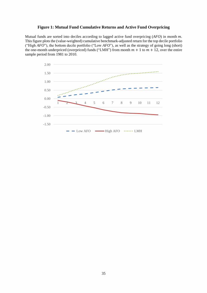
35

Figure 1: Mutual Fund Cumulative Returns and Active Fund Overpricing

Mutual funds are sorted into deciles according to lagged active fund overpricing (AFO) in month 𝑚.

This figure plots the (value-weighted) cumulative benchmark-adjusted return for the top decile portfolio

(“High AFO”), the bottom decile portfolio (“Low AFO”), as well as the strategy of going long (short)

the one-month underpriced (overpriced) funds (“LMH”) from month 𝑚 + 1 to 𝑚 + 12, over the entire

sample period from 1981 to 2010.

-1.50

-1.00

-0.50

0.00

0.50

1.00

1.50

2.00

1 2 3 4 5 6 7 8 9 10 11 12

Low AFO High AFO LMH

36

Table 1: Stock Overpricing and Stock Characteristics

Stocks are sorted into deciles according to lagged overpricing in quarter 𝑞. This table reports, for each decile portfolio, the average overpricing (Overpricing),

Log(Stock Price), Log(Stock Size), Log(Illiquidity), mutual fund ownership, analyst coverage, idiosyncratic volatility and the market share represented by each

decile portfolio in formation quarter 𝑞, as well as the average stock return in the following quarter 𝑞 + 1 over the entire sample period from 1981 to 2010. The

rows “LMH” report the difference in values between low and high overpricing portfolios (“Bottom 10% − Top 10%”). Appendix A provides the detailed

definition of each variable. Newey-West adjusted t-statistics are shown in parentheses. Numbers with “*”, “**” and “***” are significant at the 10%, 5% and

1% level, respectively.

Overpricing and Stock Characteristics

Rank of

Overpricing Overpricingq Stock Returnq+1 Market Shareq

Log (Stock

Price)q

Log (Stock

Size)q

Log (Stock

Illiquidity)q

Mutual Fund

Ownershipq

Analyst

Coverageq IdioVolq

Low 0.295 1.968 0.252 3.007 5.794 6.043 10.549 3.201 2.002

2 0.368 1.729 0.181 2.859 5.655 6.251 10.629 3.093 2.160

3 0.412 1.583 0.133 2.733 5.485 6.463 10.522 2.925 2.281

4 0.447 1.590 0.111 2.594 5.284 6.720 10.233 2.797 2.437

5 0.480 1.515 0.089 2.449 5.078 7.004 9.832 2.593 2.625

6 0.513 1.386 0.073 2.313 4.892 7.282 9.413 2.406 2.814

7 0.547 1.263 0.060 2.175 4.718 7.512 8.908 2.266 2.987

8 0.586 1.010 0.046 2.021 4.557 7.743 8.354 2.087 3.190

9 0.634 0.827 0.035 1.815 4.366 7.990 7.715 1.908 3.475

High 0.726 -0.048 0.020 1.474 4.049 8.405 6.331 1.592 4.021

LMH -0.431 2.016*** 0.232*** 1.533*** 1.745*** -2.362*** 4.219*** 1.609*** -2.019***

(7.11) (16.26) (23.46) (15.77) (-13.75) (7.81) (9.00) (-14.43)

37

Table 2: Active Fund Overpricing and Other Fund Characteristics

Mutual funds are sorted into deciles according to lagged overpricing in quarter 𝑞. This table reports, for each decile portfolio, the average active fund overpricing

(AFO) and its three components, fund return, Log(Fund TNA), Expense Ratio, Log(Fund Age), Log(Manager Tenure) and Log(Stock Illiquidity) in formation

quarter 𝑞, the average active fund overpricing (AFO) and fund flow in the following quarter 𝑞 + 1, as well as the average active fund overpricing (AFO) in

quarter 𝑞 + 4 over the entire sample period from 1981 to 2010. The rows “LMH” report the difference in values between low and high overpricing portfolios

(“Bottom 10% − Top 10%”). Appendix A provides the detailed definition of each variable. Newey-West adjusted t-statistics are shown in parentheses. Numbers

with “*”, “**” and “***” are significant at the 10%, 5% and 1% level, respectively.

Active Fund Overpricing and Other Fund Characteristics

Rank of

AFO AFOq COROPq STDASq STDOPq

Log (Fund

TNA)q

Expense

Ratioq Turnoverq

Log (Fund

Age)q

Log (Manager

Tenure)q

Log (Stock

Illiquidity)q AFOq+1

Fund

Flowq+1 AFOq+4

Low -0.043 -0.091 4.528 0.114 5.360 1.082 0.588 5.243 4.475 3.752 -0.037 0.305 -0.027

2 -0.019 -0.052 3.805 0.111 5.506 1.012 0.616 5.286 4.398 3.254 -0.016 0.256 -0.009

3 -0.009 -0.027 3.492 0.111 5.766 0.969 0.623 5.284 4.363 3.116 -0.007 0.229 -0.003

4 -0.001 -0.004 3.441 0.111 5.897 0.961 0.623 5.303 4.387 3.177 0.001 0.277 0.002

5 0.006 0.017 3.429 0.111 5.913 0.971 0.679 5.331 4.367 3.166 0.007 0.129 0.006

6 0.014 0.038 3.641 0.111 5.889 0.987 0.737 5.336 4.356 3.362 0.014 0.203 0.013

7 0.022 0.059 3.784 0.111 5.814 1.018 0.772 5.293 4.381 3.553 0.022 0.478 0.020

8 0.032 0.081 3.938 0.111 5.883 1.032 0.791 5.230 4.360 3.738 0.031 0.265 0.026

9 0.047 0.106 4.287 0.112 5.792 1.119 0.807 5.164 4.359 4.077 0.043 0.379 0.036

High 0.082 0.158 4.990 0.112 5.649 1.210 0.792 5.151 4.459 4.727 0.074 0.336 0.064

LMH -0.125 -0.250*** -0.461*** 0.002** -0.289*** -0.128*** -0.204*** 0.092 0.017 -0.974*** -0.112*** -0.031 -0.090***

(-49.53) (-4.69) (2.51) (-2.81) (-4.08) (-7.40) (1.27) (0.45) (-5.30) (-32.72) (-0.18) (-24.51)

38

Table 3: Persistence of Active Fund Overpricing

In this table, Models 1 to 5 present the results of the following quarterly Fama-MacBeth regressions, as

well as their corresponding Newey-West adjusted t-statistics,

𝐴𝐹𝑂𝑓,𝑞 = 𝛼0 + 𝛽1𝐴𝐹𝑂𝑓,𝑞−1 + 𝑐𝑀𝑓,𝑞−1 + 𝑒𝑓,𝑞,

where 𝐴𝐹𝑂𝑓,𝑞 is the active fund overpricing of fund 𝑓 in quarter 𝑞, and the vector M stacks all other

control variables, including the Lag(Fund Return), Lag(Fund Flow), Log(Fund TNA), Expense Ratio,

Turnover, Log(Fund Age), Log(Manager Tenure) and Log(Stock Illiquidity). 𝐴𝐹𝑂𝑓,𝑞−1 can be further

replaced with two dummy variables, 𝐷𝑢𝑚𝑚𝑦(𝑈𝑛𝑑𝑒𝑟𝑝𝑟𝑖𝑐𝑖𝑛𝑔)𝑓,𝑞−1 (takes a value of one if the

𝐴𝐹𝑂𝑓,𝑞−1 is in the bottom decile across all funds in that quarter and zero otherwise) and

𝐷𝑢𝑚𝑚𝑦(𝑂𝑣𝑒𝑟𝑝𝑟𝑖𝑐𝑖𝑛𝑔)𝑓,𝑞−1 (takes a value of one if the 𝐴𝐹𝑂𝑓,𝑞−1 is in the top decile across all funds

in that quarter and zero otherwise). Models 6 to 10 report similar regression parameters of the following

quarterly Fama-MacBeth regressions,

𝐴𝐹𝑂𝑓,𝑞 = 𝛼0 + 𝛽1𝐴𝐹𝑂𝑓,𝑞−4 + 𝑐𝑀𝑓,𝑞−1 + 𝑒𝑓,𝑞,

where all variables are defined as above. Appendix A provides detailed definitions for each variable.

Numbers with “*”, “**” and “***” are significant at the 10%, 5% and 1% level, respectively.

39

Table 3—Continued

Active Fund Overpricing (in %) Regressed on Lagged Active Fund Overpricing (in %)

Quarter 𝑞 − 1 Quarter 𝑞 − 4

Model 1 Model 2 Model 3 Model 4 Model 5 Model 6 Model 7 Model 8 Model 9 Model 10

AFO 0.895*** 0.878*** 0.910*** 0.719*** 0.673*** 0.736***

(106.76) (98.76) (104.42) (33.60) (29.32) (34.09) Dummy (Underpricing) -4.623*** -4.713*** -3.614*** -3.870***

(-23.06) (-19.56) (-14.81) (-13.39)

Dummy (Overpricing) 5.547*** 5.986*** 4.482*** 5.044***

(27.51) (27.65) (21.93) (24.27)

AFO × Turnover -0.049*** -0.096***

(-4.37) (-4.95) Dummy (Underpricing) × Turnover 0.116 0.310

(0.44) (1.06)

Dummy (Overpricing) × Turnover -0.514*** -0.772***

(-3.43) (-3.61)

Lag (Fund Return) -0.081*** -0.075*** -0.220*** -0.220*** -0.318*** -0.309*** -0.329*** -0.330***

(-3.27) (-3.23) (-4.48) (-4.54) (-6.04) (-6.23) (-4.96) (-4.99)

Lag (Fund Flow) 0.021*** 0.021*** 0.023** 0.023** 0.039*** 0.041*** 0.034*** 0.033***

(4.37) (4.27) (2.49) (2.44) (4.05) (4.07) (3.11) (3.05)

Log (Fund TNA) 0.027*** 0.027*** 0.159*** 0.161*** 0.101*** 0.105*** 0.193*** 0.197***

(2.74) (2.72) (4.04) (4.06) (3.49) (3.44) (4.41) (4.36)

Expense Ratio 0.129** 0.132** 0.511*** 0.536*** 0.296** 0.322** 0.600*** 0.642***

(2.24) (2.21) (4.22) (4.15) (2.12) (2.21) (3.84) (3.93)

Turnover 0.088*** 0.173*** 0.384*** 0.449*** 0.207*** 0.388*** 0.427*** 0.476***

(3.61) (4.02) (6.56) (7.26) (3.32) (4.52) (6.25) (7.24)

Log (Fund Age) -0.017 -0.013 -0.113 -0.113 -0.041 -0.041 -0.097 -0.103

(-0.75) (-0.55) (-1.59) (-1.54) (-0.73) (-0.76) (-1.15) (-1.19)

Log (Manager Tenure) 0.007 0.012 -0.025 -0.021 0.005 0.021 -0.027 -0.014

(0.44) (0.73) (-0.58) (-0.49) (0.13) (0.56) (-0.54) (-0.27)

Log (Stock Illiquidity) 0.050*** 0.051*** 0.268*** 0.266*** 0.181*** 0.176*** 0.331*** 0.329***

(3.60) (3.74) (6.23) (6.26) (4.98) (4.99) (6.16) (6.21)

Intercept 0.131*** -0.233 -0.343** -0.655 -0.733* 0.322*** -0.894** -1.086** -1.212** -1.330**

(4.31) (-1.66) (-2.09) (-1.57) (-1.70) (3.52) (-2.08) (-2.38) (-2.07) (-2.23)

R-squared 0.803 0.825 0.829 0.589 0.596 0.524 0.591 0.599 0.459 0.469

Obs 51,751 51,751 51,751 51,751 51,751 51,751 51,751 51,751 51,751 51,751

40

Table 4: Mutual Fund Returns Sorted by Active Fund Overpricing

Mutual funds are sorted into deciles according to lagged active fund overpricing (AFO) in month 𝑚.

Panel A reports the month 𝑚 + 1 (value-weighted) return for each decile portfolio as well as the

strategy of going long (short) the one-month underpriced (overpriced) funds (“LMH”) over the entire

sample period from 1981 to 2010. Fund returns are further adjusted by the benchmark return of funds,

the Morningstar style return of funds, the Daniel, Grinblatt, Titman and Wermers (1997) model, CAPM,

and Fama-French-Carhart (FFC) model. Panels B and C report similar statistics in the sub-period when

investor sentiment is high (above median) and low (below median) in month 𝑚, respectively. Appendix

A provides the detailed definition of each variable. Newey-West adjusted t-statistics are shown in

parentheses. Numbers with “*”, “**” and “***” are significant at the 10%, 5% and 1% level,

respectively.

Panel A: Returns to Investment Strategies Sorted by Active Fund Overpricing (1981 ─ 2010)

Rank of AFO Return BMK-adjusted Style-adjusted DGTW CAPM FFC

Low 0.964*** 0.089 0.093 0.078* 0.130* 0.048

(4.15) (1.38) (1.59) (1.66) (1.86) (0.79)

2 0.892*** 0.028 0.046 0.062* 0.032 -0.021

(3.69) (0.67) (1.02) (1.66) (0.74) (-0.49)

3 0.882*** 0.016 0.018 0.045 0.018 -0.034

(3.61) (0.44) (0.42) (1.33) (0.39) (-0.96)

4 0.872*** 0.036 0.044 0.012 0.016 -0.032

(3.61) (0.96) (0.93) (0.33) (0.32) (-0.80)

5 0.831*** -0.028 -0.021 -0.010 -0.033 -0.059

(3.42) (-0.76) (-0.44) (-0.28) (-0.69) (-1.27)

6 0.895*** 0.040 0.026 0.083** 0.006 -0.038

(3.47) (1.20) (0.51) (2.17) (0.12) (-0.91)

7 0.846*** -0.009 -0.019 0.022 -0.041 -0.065

(3.20) (-0.25) (-0.40) (0.54) (-0.91) (-1.44)

8 0.863*** -0.009 -0.019 0.035 -0.032 -0.037

(3.23) (-0.21) (-0.40) (0.80) (-0.61) (-0.70)

9 0.822*** -0.033 -0.034 -0.016 -0.077 -0.047

(3.01) (-0.69) (-0.65) (-0.34) (-1.14) (-0.67)

High 0.770*** -0.100* -0.081 0.018 -0.167** -0.102

(2.61) (-1.79) (-1.44) (0.36) (-2.36) (-1.52)

LMH 0.194* 0.189* 0.175* 0.060 0.297*** 0.150*

(1.73) (1.80) (1.83) (0.87) (2.97) (1.83)

41

Table 4—Continued

Panel B: Returns to Investment Strategies Sorted by Active Fund Overpricing (High Sentiment)


Low 1.096*** 0.208** 0.239*** 0.189*** 0.302*** 0.141*

(3.65) (2.11) (2.66) (2.70) (3.35) (1.94)

2 0.944*** 0.050 0.111* 0.121** 0.108* 0.034

(2.79) (0.90) (1.73) (2.35) (1.74) (0.58)

3 0.934*** 0.028 0.057 0.110** 0.099 0.007

(2.71) (0.53) (0.88) (2.23) (1.35) (0.11)

4 1.004*** 0.129** 0.175*** 0.066 0.175** 0.082

(2.98) (2.58) (2.78) (1.24) (2.35) (1.36)

5 0.876** -0.012 0.012 0.045 0.033 -0.033

(2.56) (-0.27) (0.19) (0.82) (0.47) (-0.48)

6 0.986*** 0.094* 0.145* 0.163*** 0.122* 0.007

(2.69) (1.73) (1.91) (2.67) (1.74) (0.11)

7 0.873** 0.008 0.029 0.060 0.020 -0.037

(2.39) (0.15) (0.50) (1.01) (0.29) (-0.51)

8 0.866** -0.011 0.015 0.085 0.004 -0.022

(2.37) (-0.20) (0.21) (1.38) (0.06) (-0.28)

9 0.736** -0.082 -0.075 -0.023 -0.121 -0.053

(2.03) (-1.33) (-1.12) (-0.34) (-1.33) (-0.54)

High 0.702* -0.197** -0.105 0.006 -0.205* -0.071

(1.68) (-2.27) (-1.17) (0.08) (-1.82) (-0.66)

LMH 0.394** 0.405** 0.344** 0.184* 0.507*** 0.213*

(2.07) (2.43) (2.21) (1.67) (3.19) (1.68)

Panel C: Returns to Investment Strategies Sorted by Active Fund Overpricing (Low Sentiment)


Low 0.832** -0.030 -0.052 -0.033 -0.067 -0.076

(2.34) (-0.41) (-0.81) (-0.63) (-0.92) (-1.10)

2 0.840** 0.005 -0.019 0.002 -0.049 -0.062

(2.43) (0.09) (-0.34) (0.04) (-0.94) (-1.15)

3 0.830** 0.004 -0.022 -0.020 -0.072 -0.071*

(2.37) (0.09) (-0.39) (-0.44) (-1.58) (-1.81)

4 0.740** -0.056 -0.087 -0.042 -0.152*** -0.153***

(2.13) (-1.19) (-1.44) (-0.93) (-3.28) (-3.54)

5 0.787** -0.043 -0.053 -0.066 -0.101 -0.097

(2.31) (-0.76) (-0.82) (-1.30) (-1.52) (-1.56)

6 0.805** -0.014 -0.093* 0.002 -0.112** -0.119***

(2.22) (-0.42) (-1.70) (0.06) (-2.56) (-2.85)

7 0.818** -0.025 -0.066 -0.016 -0.111** -0.108**

(2.15) (-0.58) (-0.99) (-0.27) (-2.19) (-2.08)

8 0.859** -0.006 -0.053 -0.015 -0.074 -0.089

(2.24) (-0.11) (-0.89) (-0.27) (-1.11) (-1.37)

9 0.908** 0.016 0.008 -0.009 -0.044 -0.047

(2.25) (0.23) (0.11) (-0.14) (-0.51) (-0.54)

High 0.838** -0.003 -0.057 0.030 -0.124 -0.123

(2.05) (-0.05) (-0.87) (0.51) (-1.42) (-1.52)

LMH -0.006 -0.027 0.006 -0.064 0.057 0.047

(-0.05) (-0.24) (0.06) (-0.84) (0.65) (0.55)

42

Table 5: Active Fund Overpricing and Mutual Fund Performance: Regression Analysis

This table presents the results of the following quarterly panel regressions with quarter and fund fixed

effects and their corresponding t-statistics with standard errors clustered by fund and time,

𝑃𝑒𝑟𝑓𝑓,𝑞 = 𝛼0 + 𝛽1𝐴𝐹𝑂𝑓,𝑞−1 + 𝛽2𝐴𝐹𝑂𝑓,𝑞−1 × 𝑆𝑒𝑛𝑡𝑖𝑚𝑒𝑛𝑡𝑞−1 + 𝑐𝑀𝑓,𝑞−1 + 𝑒𝑓,𝑞,

where 𝑃𝑒𝑟𝑓𝑓,𝑞 is the average monthly performance of fund 𝑓 in quarter 𝑞, 𝐴𝐹𝑂𝑓,𝑞−1 is the active fund

overpricing, 𝑆𝑒𝑛𝑡𝑖𝑚𝑒𝑛𝑡𝑞−1 is the average monthly Baker and Wurgler (2007) market sentiment index,

and the vector M stacks all other control variables, including the Active Share, (logistic transformation

of) R-square, Industry Concentration Index, Tracking Error, Lag(Fund Flow), Log(Fund TNA),

Expense Ratio, Turnover, Log(Fund Age), Log(Manager Tenure) and Log(Stock Illiquidity). 𝐴𝐹𝑂𝑓,𝑞−1

can be further replaced with its two components, 𝐶𝑂𝑅𝑂𝑃𝑓,𝑞−1 and 𝑆𝑇𝐷𝐴𝑆𝑓,𝑞−1. The dependent variable

𝑃𝑒𝑟𝑓𝑓,𝑞 is measured by raw return (Models 1 to 4) and further adjusted by the benchmark return (Models

5 to 8), as well as the Fama-French-Carhart (FFC) model (Models 9 to 12). Appendix A provides

detailed definitions for each variable. Numbers with “*”, “**”, and “***” are significant at the 10%,

5%, and 1% levels, respectively.

43

Table 5—Continued

Fund Performance (in %) Regressed on Lagged Active Fund Overpricing

Return Benchmark-adjusted Return FFC-adjusted Return

Model 1 Model 2 Model 3 Model 4 Model 5 Model 6 Model 7 Model 8 Model 9 Model 10 Model 11 Model 12

AFO -2.528** -1.484* -1.639 -2.450** -1.419* -1.482 -1.041* -0.423 -0.385

(-2.36) (-1.72) (-1.67) (-2.35) (-1.79) (-1.63) (-1.91) (-0.89) (-0.67)

COROP -0.868** -0.839* -0.400*

(-2.05) (-2.03) (-1.79) STDAS 0.033** 0.021 0.003

(2.37) (1.42) (0.29) AFO × Sentiment -3.375*** -3.281** -3.333*** -3.232** -1.997*** -1.721***

(-3.14) (-2.37) (-3.01) (-2.29) (-3.51) (-2.87)

Active Share 0.656* 0.595* 0.148

(1.75) (1.95) (0.74)

TR2 -0.027 -0.001 0.003

(-0.89) (-0.06) (0.23)

ICI 0.322 0.379 -0.455

(0.40) (0.58) (-1.24)

Tracking Error -0.014 -0.003 0.005

(-0.60) (-0.12) (0.27)

Lag (Fund Flow) -0.003 -0.003 -0.003 -0.005 -0.002 -0.002 -0.001 -0.002 -0.000 -0.000 -0.000 -0.001

(-1.51) (-1.48) (-1.44) (-1.14) (-1.06) (-1.02) (-0.99) (-0.60) (-0.49) (-0.47) (-0.45) (-0.30)

Log (Fund TNA) -0.267*** -0.266*** -0.263*** -0.267*** -0.241*** -0.241*** -0.237*** -0.242*** -0.149*** -0.149*** -0.147*** -0.156***

(-5.75) (-5.72) (-5.64) (-5.90) (-6.18) (-6.17) (-6.04) (-6.36) (-8.88) (-8.63) (-8.83) (-8.75)

Expense Ratio -0.117** -0.114** -0.119** -0.145** -0.083 -0.079 -0.084* -0.103* -0.022 -0.020 -0.023 -0.051

(-2.25) (-2.16) (-2.32) (-2.20) (-1.66) (-1.56) (-1.75) (-1.78) (-0.65) (-0.58) (-0.69) (-1.39)

Turnover 0.023 0.024 0.022 0.019 0.021 0.021 0.020 0.018 -0.013 -0.012 -0.013 -0.019

(1.06) (1.14) (1.08) (0.68) (0.94) (0.99) (0.95) (0.68) (-0.55) (-0.53) (-0.57) (-0.68)

Log (Fund Age) 0.040 0.045 0.038 0.043 0.050 0.054 0.048 0.065 0.002 0.003 0.001 0.001

(0.69) (0.77) (0.64) (0.65) (1.25) (1.34) (1.19) (1.39) (0.06) (0.10) (0.02) (0.03)

Log (Manager Tenure) -0.004 -0.006 -0.003 0.001 -0.006 -0.007 -0.005 -0.002 -0.000 -0.000 0.001 0.004

(-0.24) (-0.35) (-0.15) (0.05) (-0.42) (-0.50) (-0.32) (-0.10) (-0.03) (-0.05) (0.06) (0.45)

Log (Stock Illiquidity) 0.121*** 0.112** 0.116*** 0.104*** 0.094** 0.087** 0.089** 0.077** 0.028** 0.027*** 0.025** 0.027**

(2.90) (2.76) (2.89) (2.79) (2.54) (2.45) (2.52) (2.41) (2.66) (2.77) (2.75) (2.60)

R-squared 0.852 0.852 0.852 0.845 0.072 0.072 0.076 0.079 0.137 0.137 0.140 0.146

Obs 53,765 53,756 53,765 45,092 53,765 53,756 53,765 45,092 53,765 53,756 53,765 45,092

44

Table 6: Mutual Fund Returns Adjusted by Mispricing Factors

In Panel A, mutual funds are sorted into deciles according to lagged active fund overpricing (AFO) in month 𝑚. We report the month 𝑚 + 1 (value-weighted)

performance for each decile portfolio as well as the strategy of going long (short) the one-month underpriced (overpriced) funds (“LMH”) over the entire sample

period from 1981 to 2010. Fund returns are adjusted by the Stambaugh and Yuan (2017) model, including the market factor (RMRF), the size factor (SMB),

and two mispricing factors arising from cluster of anomalies related to firms’ managements (MGMT) and performance (PERF). Panel B Models 1 to 4 present

the results of the following quarterly panel regressions with quarter and fund fixed effects and their corresponding t-statistics with standard errors clustered by

fund and time,


where 𝑃𝑒𝑟𝑓𝑓,𝑞 is the average monthly Stambaugh and Yuan (2017) four-factor-adjusted return of fund 𝑓 in quarter 𝑞, 𝐴𝐹𝑂𝑓,𝑞−1 is the active fund overpricing,

𝑆𝑒𝑛𝑡𝑖𝑚𝑒𝑛𝑡𝑞−1 is the average monthly Baker and Wurgler (2007) market sentiment index, and the vector M stacks all other control variables, including the

Active Share, (logistic transformation of) R-square, Industry Concentration Index, Tracking Error, Lag(Fund Flow), Log(Fund TNA), Expense Ratio, Turnover,

Log(Fund Age), Log(Manager Tenure) and Log(Stock Illiquidity). 𝐴𝐹𝑂𝑓,𝑞−1 can be further replaced with its two components, 𝐶𝑂𝑅𝑂𝑃𝑓,𝑞−1 and 𝑆𝑇𝐷𝐴𝑆𝑓,𝑞−1.

Appendix A provides detailed definitions for each variable. Numbers with “*”, “**”, and “***” are significant at the 10%, 5%, and 1% levels, respectively.

Panel A: Mispricing Factor-Adjusted Returns to Investment Strategies Sorted by Active Fund Overpricing

Low 2 3 4 5 6 7 8 9 High LMH

Intercept -0.045 -0.076* -0.090** -0.088* -0.088* -0.102** -0.078 -0.034 -0.002 0.033 -0.078

(-0.66) (-1.65) (-2.22) (-1.93) (-1.77) (-2.28) (-1.45) (-0.60) (-0.02) (0.50) (-0.92)

RMRF 0.895*** 0.941*** 0.954*** 0.937*** 0.937*** 0.995*** 0.960*** 0.958*** 0.932*** 0.941*** -0.047

(40.73) (59.51) (68.34) (61.67) (61.83) (60.64) (61.78) (61.56) (32.64) (46.03) (-1.53)

SMB 0.108*** -0.010 -0.027 -0.030 -0.045* 0.019 0.033 0.058 0.079*** 0.185*** -0.077**

(3.07) (-0.29) (-1.18) (-1.42) (-1.66) (0.61) (1.09) (1.61) (2.70) (5.50) (-1.98)

MGMT 0.137*** 0.092*** 0.101*** 0.105*** 0.053** 0.077*** 0.017 -0.010 -0.083** -0.188*** 0.325***

(4.30) (4.18) (4.59) (4.03) (2.39) (3.07) (0.62) (-0.40) (-2.55) (-7.71) (8.25)

PERF 0.024 0.032* 0.028* 0.022 0.023 0.036** 0.013 -0.007 -0.027 -0.094*** 0.117***

(1.13) (1.95) (1.83) (1.33) (1.24) (2.14) (0.75) (-0.49) (-1.38) (-5.03) (3.59)

Obs 348 348 348 348 348 348 348 348 348 348 348

45

Table 6—Continued

Panel B: Mispricing Factor-Adjusted Fund Performance (in %) Regressed on Lagged Active Fund Overpricing

Model 1 Model 2 Model 3 Model 4

AFO -0.535 -0.003 0.104

(-0.95) (-0.01) (0.18)

COROP -0.188

(-0.82)

STDAS 0.008

(0.50)

AFO × Sentiment -1.717*** -1.440*

(-2.95) (-1.93)

Active Share -0.012

(-0.04)

TR2 0.019

(1.12)

ICI 0.138

(0.25)

Tracking Error 0.008

(0.36)

Lag (Fund Flow) -0.002 -0.002 -0.002 -0.003

(-1.43) (-1.44) (-1.39) (-1.12)

Log (Fund TNA) -0.148*** -0.147*** -0.146*** -0.155***

(-9.58) (-9.55) (-9.37) (-9.76)

Expense Ratio -0.084* -0.083* -0.084* -0.130**

(-1.79) (-1.75) (-1.84) (-2.46)

Turnover -0.031 -0.031 -0.031 -0.031

(-0.92) (-0.91) (-0.93) (-0.83)

Log (Fund Age) 0.001 0.003 0.000 0.001

(0.04) (0.08) (0.01) (0.02)

Log (Manager Tenure) 0.006 0.006 0.007 0.011

(0.50) (0.46) (0.56) (0.98)

Log (Stock Illiquidity) 0.017 0.015 0.014 0.020

(1.12) (1.08) (0.96) (1.53)

R-squared 0.149 0.149 0.151 0.158

Obs 53,765 53,756 53,765 45,092

46

Table 7: Active Fund Overpricing and Flows

This table presents the results of the following quarterly panel regressions with quarter and fund fixed effects and their

corresponding t-statistics with standard errors clustered by fund and time,

𝐹𝑙𝑜𝑤𝑓,𝑞 = 𝛼0 + 𝛽1𝐴𝐹𝑂𝑓,𝑞−1 + 𝛽2𝐴𝐹𝑂𝑓,𝑞−1 × 𝑆𝑒𝑛𝑡𝑖𝑚𝑒𝑛𝑡𝑞−1 + 𝛽3𝑃𝑒𝑟𝑓𝑓,𝑞−1 + 𝑐𝑀𝑓,𝑞−1 + 𝑒𝑓,𝑞,

where 𝐹𝑙𝑜𝑤𝑓,𝑞 refers to the average monthly flow (Models 1 to 4) and benchmark-adjusted flow (Models 5 to 8) of fund

𝑓 in quarter 𝑞, 𝐴𝐹𝑂𝑓,𝑞−1 is the active fund overpricing, 𝑆𝑒𝑛𝑡𝑖𝑚𝑒𝑛𝑡𝑞−1 is the average monthly Baker and Wurgler (2007)

market sentiment index, 𝑃𝑒𝑟𝑓𝑓,𝑞−1 is the average monthly fund return, and the vector M stacks all other control variables,

including the Active Share, (logistic transformation of) R-square, Industry Concentration Index, Tracking Error,

Lag(Fund Flow), Log(Fund TNA), Expense Ratio, Turnover, Log(Fund Age) and Log(Manager Tenure). Appendix A

provides detailed definitions for each variable. Numbers with “*”, “**”, and “***” are significant at the 10%, 5%, and

1% levels, respectively.

Fund Flow (in %) Regressed on Lagged Active Fund Overpricing

Flow Benchmark-adjusted Fund Flow

Model 1 Model 2 Model 3 Model 4 Model 5 Model 6 Model 7 Model 8

AFO 1.770* 1.045 1.572* 1.206 1.980** 1.319 1.805* 1.445*

(1.99) (1.15) (1.81) (1.58) (2.17) (1.45) (2.03) (1.85)

AFO × Sentiment 2.688** 0.969 2.453** 0.737

(2.50) (0.91) (2.30) (0.72)

Fund Returnq-1 × Sentiment -0.157*** -0.141*** -0.139*** -0.125***

(-6.41) (-7.62) (-7.30) (-8.20)

Active Share 0.510 0.534

(1.26) (1.36)

TR2 0.057** 0.072***

(2.69) (2.99)

ICI -1.072 -0.733

(-1.03) (-0.73)

Tracking Error -0.031 -0.035*

(-1.40) (-1.71)

Lag (Fund Flow) 0.126 0.125 0.124 0.317*** 0.127 0.127 0.126 0.324***

(1.58) (1.58) (1.58) (13.30) (1.57) (1.57) (1.57) (13.08)

Fund Returnq-1 0.275*** 0.278*** 0.356*** 0.322*** 0.249*** 0.252*** 0.321*** 0.293***

(4.26) (4.36) (7.81) (8.91) (4.70) (4.80) (8.12) (9.11)

Fund Returnq-4:q-2 0.565*** 0.573*** 0.596*** 0.438*** 0.550*** 0.557*** 0.577*** 0.424***

(4.26) (4.36) (4.84) (4.93) (4.41) (4.50) (4.91) (4.90)

Log (Fund TNA) -0.598*** -0.601*** -0.615*** -0.670*** -0.600*** -0.603*** -0.615*** -0.665***

(-8.26) (-8.28) (-8.73) (-9.00) (-8.55) (-8.56) (-8.97) (-9.06)

Expense Ratio 0.093 0.093 0.115 -0.184 0.084 0.084 0.104 -0.192

(0.45) (0.45) (0.55) (-1.17) (0.40) (0.40) (0.49) (-1.21)

Turnover -0.021 -0.021 -0.022 -0.060 -0.039 -0.038 -0.039 -0.070

(-0.35) (-0.34) (-0.36) (-1.09) (-0.60) (-0.59) (-0.61) (-1.24)

Log (Fund Age) -1.212*** -1.212*** -1.205*** -0.820*** -1.100*** -1.100*** -1.094*** -0.724***

(-5.49) (-5.49) (-5.55) (-5.20) (-5.20) (-5.20) (-5.25) (-4.55)

Log (Manager Tenure) 0.115*** 0.114*** 0.119*** 0.097** 0.122*** 0.121*** 0.126*** 0.102***

(2.94) (2.92) (3.14) (2.68) (3.23) (3.21) (3.40) (2.89)

R-squared 0.276 0.276 0.280 0.344 0.266 0.266 0.269 0.335

Obs 55,901 55,901 55,901 45,092 55,901 55,901 55,901 45,092

47

Table IA1: Summary Statistics

This table presents the summary statistics for the data used in the paper during the 1981–2010 period.

We report the mean, median, standard deviation, and the quantile distribution of quarterly fund

overpricing, monthly fund return, monthly fund flow, and other quarterly stock and fund characteristics.

Appendix A provides the detailed definition of each variable.

Quantile Distribution of Fund Characteristics

Mean Std.Dev. Quantile Distribution

10% 25% Median 75% 90%

AFO 0.008 0.035 -0.030 -0.012 0.005 0.025 0.049

COROP 0.015 0.079 -0.078 -0.033 0.012 0.060 0.110

STDAS 3.883 1.717 2.202 2.789 3.604 4.606 5.841

STDOP 0.113 0.009 0.102 0.108 0.114 0.119 0.124

Fund Return 0.575 3.233 -3.770 -1.008 0.892 2.494 4.356

BMK-adjusted 0.001 1.144 -1.217 -0.564 -0.016 0.553 1.241

DGTW-adjusted -0.015 1.043 -1.144 -0.503 -0.013 0.477 1.109

FFC-adjusted -0.128 0.879 -1.156 -0.610 -0.129 0.353 0.895

Mispricing-adjusted -0.110 0.935 -1.210 -0.611 -0.100 0.397 0.949

Fund Flow 0.037 3.420 -2.660 -1.392 -0.409 0.847 3.076

BMK-adjusted -0.562 3.392 -3.377 -2.063 -0.901 0.333 2.424

Active Share 0.787 0.154 0.573 0.685 0.812 0.918 0.967

TR2 3.794 1.254 2.396 2.955 3.625 4.453 5.424

ICI 0.042 0.048 0.008 0.017 0.031 0.051 0.082

Tracking Error 1.372 1.176 0.364 0.626 1.067 1.745 2.683

Log (Fund TNA) 5.862 1.641 3.726 4.610 5.795 6.994 8.084

Expense Ratio 1.190 0.397 0.720 0.947 1.168 1.423 1.718

Turnover 0.774 0.656 0.167 0.310 0.600 1.020 1.590

Log (Fund Age) 4.979 0.716 4.111 4.440 4.877 5.407 6.094

Log (Manager Tenure) 4.315 0.734 3.296 3.932 4.367 4.764 5.176

Log (Stock Illiquidity) 2.323 2.236 -0.209 0.435 1.848 3.821 5.537

48

Table IA2: Active Fund Overpricing and Mutual Fund Performance: Robustness

Checks

Models 1 to 6 present the results of the following quarterly panel regressions with quarter fixed effects

and their corresponding t-statistics with standard errors clustered by fund and time,






Expense Ratio, Turnover, Log(Fund Age), Log(Manager Tenure) and Log(Stock Illiquidity). The

dependent variable 𝑃𝑒𝑟𝑓𝑓,𝑞 is measured by raw return (Models 1 to 2) and further adjusted by the

benchmark return (Models 3 to 4), as well as the Fama-French-Carhart (FFC) model (Models 5 to 6).

Models 7 to 12 report similar regression parameters of the quarterly Fama-MacBeth regressions as well

as their corresponding Newey-West adjusted t-statistics. Appendix A provides detailed definitions for

each variable. Numbers with “*”, “**”, and “***” are significant at the 10%, 5%, and 1% levels,

respectively.

49

Table IA2—Continued

Fund Performance (in %) Regressed on Lagged Active Fund Overpricing

Return BMK-adjusted FFC-adjusted Return BMK-adjusted FFC-adjusted


AFO -0.702 -0.858 -0.327 -0.486 0.005 -0.017 -0.450 -0.817 -0.265 -0.698 -0.379 -0.654

(-0.66) (-0.76) (-0.37) (-0.51) (0.01) (-0.03) (-0.78) (-1.34) (-0.46) (-1.12) (-1.12) (-1.59)

AFO × Sentiment -3.878*** -3.744*** -3.943*** -3.775*** -2.438*** -2.163*** -0.957** -0.731* -0.900** -0.661* -0.597** -0.450*

(-3.64) (-2.83) (-3.73) (-2.89) (-4.45) (-3.87) (-2.39) (-1.97) (-2.24) (-1.82) (-2.57) (-1.98)

Active Share 0.457* 0.341* 0.080 -0.064 -0.124 -0.002

(1.81) (1.80) (0.42) (-0.27) (-0.58) (-0.01)

TR2 -0.029 -0.015 -0.016 -0.004 -0.007 -0.011

(-0.85) (-0.50) (-1.26) (-0.19) (-0.31) (-1.00)

ICI -0.078 0.172 -0.143 0.377 0.526 -0.244

(-0.18) (0.38) (-0.60) (0.83) (1.12) (-0.82)

Tracking Error -0.016 -0.001 0.003 -0.007 -0.011 -0.015

(-0.56) (-0.05) (0.15) (-0.39) (-0.69) (-1.28)

Lag (Fund Flow) 0.002 0.005 0.003 0.007* 0.003 0.007*** 0.005 0.008 0.008* 0.008 0.007** 0.006

(0.60) (1.03) (1.02) (1.71) (1.52) (2.81) (1.09) (1.41) (1.82) (1.47) (2.10) (1.61)

Log (Fund TNA) -0.015 -0.011 -0.016 -0.014 -0.004 -0.004 0.002 0.007 -0.000 0.005 0.008 0.013*

(-1.31) (-1.07) (-1.66) (-1.56) (-0.99) (-0.76) (0.28) (0.88) (-0.06) (0.64) (1.17) (1.72)

Expense Ratio -0.086** -0.131*** -0.084*** -0.111*** -0.059*** -0.074*** -0.038 -0.029 -0.046 -0.023 -0.046 -0.034

(-2.67) (-3.27) (-3.14) (-3.07) (-2.77) (-3.88) (-1.09) (-0.67) (-1.43) (-0.52) (-1.62) (-1.07)

Turnover -0.007 -0.004 -0.032 -0.030 -0.049 -0.050 0.052 0.065 0.031 0.044 -0.017 -0.011

(-0.15) (-0.07) (-0.79) (-0.62) (-1.49) (-1.31) (1.26) (1.42) (0.96) (1.16) (-0.79) (-0.41)

Log (Fund Age) 0.014 0.014 0.025* 0.029** 0.000 0.002 0.007 0.005 0.014 0.013 -0.013 -0.002

(1.12) (1.14) (1.91) (2.18) (0.00) (0.23) (0.45) (0.33) (0.88) (0.89) (-1.06) (-0.14)

Log (Manager Tenure) -0.009 -0.012 0.000 -0.002 0.007 0.005 -0.018 -0.019 -0.015 -0.018 -0.008 -0.011

(-0.71) (-0.86) (0.02) (-0.12) (0.64) (0.54) (-1.29) (-1.23) (-1.02) (-1.26) (-0.80) (-1.00)

Log (Stock Illiquidity) 0.081** 0.061** 0.036** 0.020 0.005 0.000 0.049* 0.058*** 0.026 0.037** 0.023** 0.031***

(2.66) (2.10) (2.14) (1.26) (0.56) (0.05) (1.82) (2.74) (1.33) (2.32) (2.45) (2.79)

Regression Panel Fama-MacBeth

R-squared 0.845 0.837 0.025 0.028 0.087 0.093 0.223 0.316 0.156 0.248 0.118 0.197

Obs 53,782 45,112 53,782 45,112 53,782 45,112 53,782 45,112 53,782 45,112 53,782 45,112

50

Table IA3: Active Fund Overpricing and Alternative Mutual Fund Performance

This table presents the results of the following quarterly panel regressions with quarter and fund fixed

effects and their corresponding t-statistics with standard errors clustered by fund and time,






Expense Ratio, Turnover, Log(Fund Age), Log(Manager Tenure) and Log(Stock Illiquidity). 𝐴𝐹𝑂𝑓,𝑞−1

can be further replaced with its two components, 𝐶𝑂𝑅𝑂𝑃𝑓,𝑞−1 and 𝑆𝑇𝐷𝐴𝑆𝑓,𝑞−1. The dependent variable

𝑃𝑒𝑟𝑓𝑓,𝑞 is measured by Daniel, Grinblatt, Titman and Wermers (1997) characteristics adjusted return

(Models 1 to 4), the product of gross-of-fee benchmark-adjusted return in quarter 𝑞 and the assets under

management (adjusted by inflation, expressed in January 1, 2000 USD) in quarter 𝑞 − 1, following

Berk and van Binsbergen (2015) (Models 5 to 8), and the average monthly abnormal return gap during

3-year interval (Models 9 to 12). The monthly return gap is computed as the difference between fund

gross-of-fee return and holding-based return, where gross-of-fee return is the fund total return plus one-

twelfth of the annualized expense ratio, and holding-based return is the investment value-weighted

average of stock returns of a fund’s most recently reported holding portfolio. Furthermore, the monthly

abnormal return gap is computed using a four-factor (market, size, book-to-market, and momentum)

model, following Kacperczyk, Sialm, and Zheng (2008). Appendix A provides detailed definitions for

each variable. Numbers with “*”, “**”, and “***” are significant at the 10%, 5%, and 1% levels,

respectively.

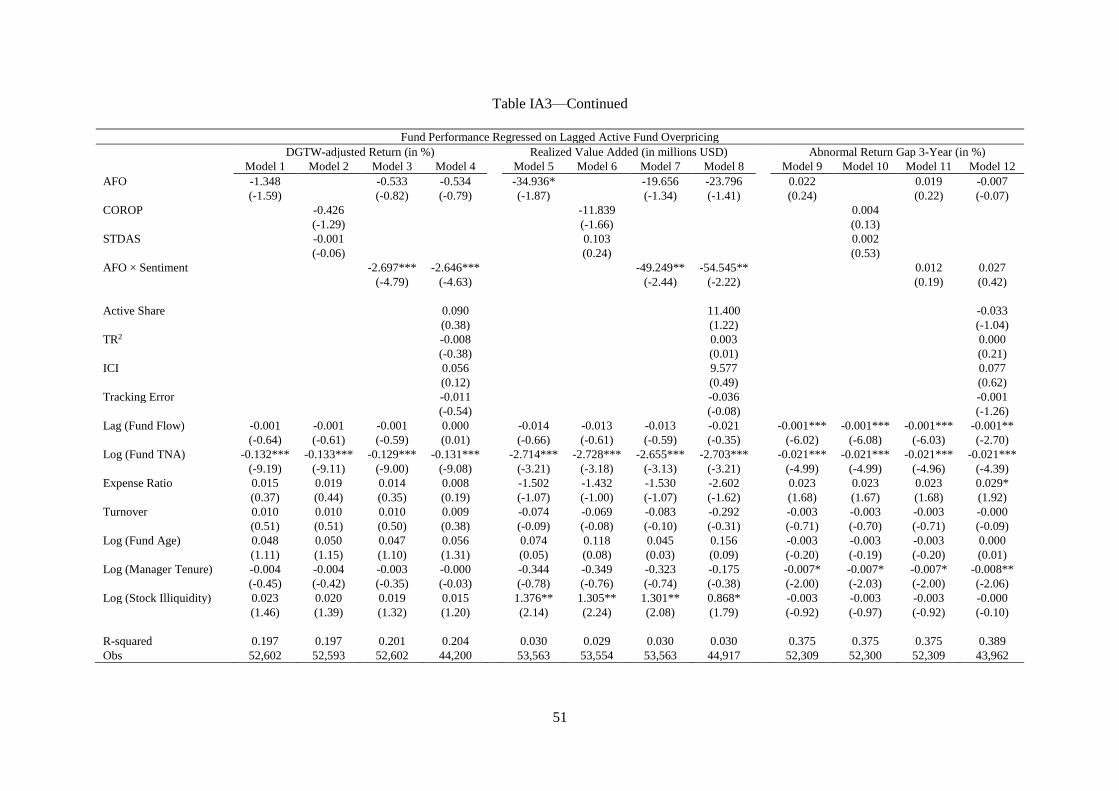
51

Table IA3—Continued

Fund Performance Regressed on Lagged Active Fund Overpricing

DGTW-adjusted Return (in %) Realized Value Added (in millions USD) Abnormal Return Gap 3-Year (in %)


AFO -1.348 -0.533 -0.534 -34.936* -19.656 -23.796 0.022 0.019 -0.007

(-1.59) (-0.82) (-0.79) (-1.87) (-1.34) (-1.41) (0.24) (0.22) (-0.07)

COROP -0.426 -11.839 0.004

(-1.29) (-1.66) (0.13) STDAS -0.001 0.103 0.002

(-0.06) (0.24) (0.53) AFO × Sentiment -2.697*** -2.646*** -49.249** -54.545** 0.012 0.027

(-4.79) (-4.63) (-2.44) (-2.22) (0.19) (0.42)

Active Share 0.090 11.400 -0.033

(0.38) (1.22) (-1.04)

TR2 -0.008 0.003 0.000

(-0.38) (0.01) (0.21)

ICI 0.056 9.577 0.077

(0.12) (0.49) (0.62)

Tracking Error -0.011 -0.036 -0.001

(-0.54) (-0.08) (-1.26)

Lag (Fund Flow) -0.001 -0.001 -0.001 0.000 -0.014 -0.013 -0.013 -0.021 -0.001*** -0.001*** -0.001*** -0.001**

(-0.64) (-0.61) (-0.59) (0.01) (-0.66) (-0.61) (-0.59) (-0.35) (-6.02) (-6.08) (-6.03) (-2.70)

Log (Fund TNA) -0.132*** -0.133*** -0.129*** -0.131*** -2.714*** -2.728*** -2.655*** -2.703*** -0.021*** -0.021*** -0.021*** -0.021***

(-9.19) (-9.11) (-9.00) (-9.08) (-3.21) (-3.18) (-3.13) (-3.21) (-4.99) (-4.99) (-4.96) (-4.39)

Expense Ratio 0.015 0.019 0.014 0.008 -1.502 -1.432 -1.530 -2.602 0.023 0.023 0.023 0.029*

(0.37) (0.44) (0.35) (0.19) (-1.07) (-1.00) (-1.07) (-1.62) (1.68) (1.67) (1.68) (1.92)

Turnover 0.010 0.010 0.010 0.009 -0.074 -0.069 -0.083 -0.292 -0.003 -0.003 -0.003 -0.000

(0.51) (0.51) (0.50) (0.38) (-0.09) (-0.08) (-0.10) (-0.31) (-0.71) (-0.70) (-0.71) (-0.09)

Log (Fund Age) 0.048 0.050 0.047 0.056 0.074 0.118 0.045 0.156 -0.003 -0.003 -0.003 0.000

(1.11) (1.15) (1.10) (1.31) (0.05) (0.08) (0.03) (0.09) (-0.20) (-0.19) (-0.20) (0.01)

Log (Manager Tenure) -0.004 -0.004 -0.003 -0.000 -0.344 -0.349 -0.323 -0.175 -0.007* -0.007* -0.007* -0.008**

(-0.45) (-0.42) (-0.35) (-0.03) (-0.78) (-0.76) (-0.74) (-0.38) (-2.00) (-2.03) (-2.00) (-2.06)

Log (Stock Illiquidity) 0.023 0.020 0.019 0.015 1.376** 1.305** 1.301** 0.868* -0.003 -0.003 -0.003 -0.000

(1.46) (1.39) (1.32) (1.20) (2.14) (2.24) (2.08) (1.79) (-0.92) (-0.97) (-0.92) (-0.10)

R-squared 0.197 0.197 0.201 0.204 0.030 0.029 0.030 0.030 0.375 0.375 0.375 0.389

Obs 52,602 52,593 52,602 44,200 53,563 53,554 53,563 44,917 52,309 52,300 52,309 43,962

Documents

Mutual Funds and Mispriced Stocks