Embed Size (px)
Citation preview

MWANGI STANLEY NJENGA
BANDLIMITED DIGITAL PREDISTORTION OF WIDEBAND
RF POWER AMPLIFIERS
Master of Science Thesis
Examiner: Prof. Mikko ValkamaExaminer and topic approved by theFaculty Council of the Faculty ofComputing and Electrical Engineeringon 31st May 2017

i
ABSTRACT
MWANGI STANLEY NJENGA: BandLimited Digital Predistortion of WidebandRF Power AmplifiersTampere University of TechnologyMaster of Science Thesis, 68 pages, 2 Appendix pagesMaster’s Degree Programme in Electrical EngineeringMajor: Wireless CommunicationsExaminer: Prof. Mikko ValkamaKeywords: Adaptive filters, behavioral modeling, carrier aggregation, digital predistor-tion, LTE/LTE-A, nonlinear distortion, power amplifiers.
The increase in the demand for high data rates has led to the deployment of widerbandwidths and complex waveforms in wireless communication systems. Multicar-rier waveforms such as orthogonal frequency division multiplexing (OFDM) em-ployed in modern systems are very sensitive to the transmitter chain nonideali-ties due to their high peak-to-average-power-ratio (PAPR) characteristic. Theyare therefore affected by nonlinear transmitter components particularly the poweramplifier (PA). Moreover, to enhance power efficiency, PAs typically operate nearsaturation region and hence become more nonlinear. Power efficiency is highly de-sirable especially in battery powered and portable devices as well as in base stations.Hence there is a clear need for efficient linearization algorthms which improve powerefficiency while maintaining high spectral efficiency.
Digital predistortion (DPD) has been recognized as one of the most effective meth-ods in mitigating PA nonlinear distortions. The method involves the applicationof inverse PA nonlinear function upstream of the PA such that the overall systemoutput has a linear amplification. The computation of the nonlinearity profile andthe inversion of the PA function are particularly difficult and complicated especiallywhen involving wideband radio access waveforms, and therefore memory effects,which are being employed in modern communication systems, such as in Long TermEvolution/Advanced (LTE/LTE-A). In the recent technical literature, different ap-proaches which focus on the linearization of specific frequency bands or sub-bandsonly have been developed to alleviate this problem, thereby reducing the complexityof DPD.
In this thesis, we focus on the development and characterization of a bandlimited

ii
DPD solution specifically tailored towards the linearization at and around the maincarrier(s) in single carrier deployment or contiguous carrier aggregation of two ormore component carriers. In terms of parameter identification, the solution is basedon the reduced-complexity closed-loop decorrelation-based parameter learning prin-ciple, which is also able to track time-varying changes in the transmitter componentsadaptively. The proposed bandlimited solution is designed to linearize the inbandand out-of-band (OOB) distortions in the immediate vicinity of the main carrier(s)while assuming the distortions more far away in the spectrum are suppressed bytransmit or duplex filters. This is implemented using FIR filters to limit the band-width expansion during basis functions generation and to restrain the bandwidth ofthe feedback observation signal, thus reducing the DPD sample rates in both themain path processing and the parameter learning. The performance of the proposedbandlimited DPD solution is evaluated using comprehensive simulations involvingmemoryless and memory-based PA models, as well as true RF measurements us-ing commercial LTE-A base station and mobile device PAs. The achieved resultsvalidate and demonstrate efficient suppression of inband and OOB distortions inreal-world application scenarios. Furthermore, the bandlimited DPD consistentlyoutperforms the conventional DPD solutions in the memory-based PA model andpractical PA scenarios in suppressing the OOB distortion in the immediate vicin-ity of the main carrier(s) by approximately 1 - 2 dB. The results provide sufficientgrounds for the application of the bandlimited DPD solution in the classical singlecarrier deployment or in contiguous carrier aggregation of two or more componentcarriers where conventional DPD solutions would otherwise be highly complex.

iii
PREFACE
This thesis work was carried out at the Department of Electronics and Communica-tion Engineering, Tampere University of Technology, Finland. First of all, I wouldlike to thank Prof. Mikko Valkama for accepting me to join his research group andguiding me through the research work. I am also very grateful to MSc. MahmoudAbdelaziz and Dsc. Adnan Kiayani for the advice, guidance, support, and patiencethey gave me in the entire period of the work. Special thanks to my colleaguesZeeshan Waheed and Weijie Zhu for their company and assistance during the thesisperiod and course work.
My study in Finland was generously supported by my parents, Mr. Sammy Mbuguaand Mrs. Ann Mwangi, and I will always be indebted for their love and care duringmy education. I am also glad to my brothers for the unwaning encouragement andsupport. This thesis work was also supported by Nokia Bells Labs and Tekes throughthe 5G-TRX research project.
Special thanks go to all my friends I met in Tampere and overall in Finland; Ferdi-nand Muriyesu, Alain Itangishaka, Eunice Kamau, Simon Kamau, Joseph Gichuru,and Edward Amayo, among others.
I will forever be grateful to Finland and Tampere University of Technology for of-fering me an opportunity to study and enjoy tuition-free yet high-quality education.
Tampere, 6.9.2017
Stanley Mwangi

iv
TABLE OF CONTENTS
1. Introduction . . . . . . . . . . . . . . . . . . . . . . . . . . . . . . . . . . . 1
1.1 Background and Motivation . . . . . . . . . . . . . . . . . . . . . . . 1
1.2 Scope and Outline of the Thesis . . . . . . . . . . . . . . . . . . . . . 5
2. Power Amplifier Behavioral Modeling . . . . . . . . . . . . . . . . . . . . . 7
2.1 Memoryless Nonlinear Models . . . . . . . . . . . . . . . . . . . . . . 7
2.1.1 Memoryless Polynomial Model . . . . . . . . . . . . . . . . . . . 9
2.1.2 Saleh Model . . . . . . . . . . . . . . . . . . . . . . . . . . . . . 10
2.1.3 Ghorbani Model . . . . . . . . . . . . . . . . . . . . . . . . . . . 11
2.1.4 Rapp Model . . . . . . . . . . . . . . . . . . . . . . . . . . . . . 11
2.1.5 White Model . . . . . . . . . . . . . . . . . . . . . . . . . . . . . 11
2.2 Memory-Based Nonlinear Models . . . . . . . . . . . . . . . . . . . . 12
2.2.1 Volterra Series . . . . . . . . . . . . . . . . . . . . . . . . . . . . 13
2.2.2 Memory Polynomial Model . . . . . . . . . . . . . . . . . . . . . 16
2.2.3 Wiener Model . . . . . . . . . . . . . . . . . . . . . . . . . . . . 17
2.2.4 Hammerstein Model . . . . . . . . . . . . . . . . . . . . . . . . . 18
2.2.5 Wiener - Hammerstein Model . . . . . . . . . . . . . . . . . . . . 19
2.2.6 Saleh Memory-Based Model . . . . . . . . . . . . . . . . . . . . . 20
2.3 Discussion . . . . . . . . . . . . . . . . . . . . . . . . . . . . . . . . . 20
3. Effects and Mitigation of Power Amplifiers Nonlinearity . . . . . . . . . . . 22
3.1 Effects of Power Amplifier Nonlinearity . . . . . . . . . . . . . . . . . 22
3.2 Feedback Linearization . . . . . . . . . . . . . . . . . . . . . . . . . . 25
3.3 Feedforward Linearization . . . . . . . . . . . . . . . . . . . . . . . . 27
3.4 LINC . . . . . . . . . . . . . . . . . . . . . . . . . . . . . . . . . . . . 28
3.5 CALLUM . . . . . . . . . . . . . . . . . . . . . . . . . . . . . . . . . 29
3.6 Digital Predistortion . . . . . . . . . . . . . . . . . . . . . . . . . . . 30

v
3.6.1 Direct Learning Architecture . . . . . . . . . . . . . . . . . . . . 30
3.6.2 Indirect Learning Architecture . . . . . . . . . . . . . . . . . . . 32
3.6.3 Closed Loop Adaptive Digital Predistortion . . . . . . . . . . . . 32
3.7 Discussion . . . . . . . . . . . . . . . . . . . . . . . . . . . . . . . . . 33
4. BandLimited Digital Predistortion . . . . . . . . . . . . . . . . . . . . . . 35
4.1 Basics of Sampling and Filtering Theory . . . . . . . . . . . . . . . . 36
4.2 Digital Predistortion Modeling . . . . . . . . . . . . . . . . . . . . . . 39
4.2.1 Basis Functions Generation and Orthogonalization . . . . . . . . 39
4.2.2 Basis Functions and Receiver Feedback Filtering . . . . . . . . . 40
4.2.3 Distortion Components Modeling . . . . . . . . . . . . . . . . . . 41
4.3 DPD Parameter Learning Algorithm . . . . . . . . . . . . . . . . . . 43
4.3.1 Sample-Adaptive Decorrelation Based Learning . . . . . . . . . . 44
4.3.2 Block Adaptive Decorrelation-Based Learning . . . . . . . . . . . 45
5. Simulation and Measurement Results . . . . . . . . . . . . . . . . . . . . . 47
5.1 Matlab Simulations . . . . . . . . . . . . . . . . . . . . . . . . . . . . 47
5.1.1 Simulation Parameters . . . . . . . . . . . . . . . . . . . . . . . . 47
5.1.2 Simulation Results . . . . . . . . . . . . . . . . . . . . . . . . . . 49
5.2 RF Measurements . . . . . . . . . . . . . . . . . . . . . . . . . . . . . 51
5.2.1 Hardware Description and Measurement Setup . . . . . . . . . . 53
5.2.2 UE Measurement Results . . . . . . . . . . . . . . . . . . . . . . 55
5.2.3 Base Station Measurement Results . . . . . . . . . . . . . . . . . 56
5.3 Discussion . . . . . . . . . . . . . . . . . . . . . . . . . . . . . . . . . 58
6. Conclusion . . . . . . . . . . . . . . . . . . . . . . . . . . . . . . . . . . . . 61
Bibliography . . . . . . . . . . . . . . . . . . . . . . . . . . . . . . . . . . . . 63
APPENDIX A . . . . . . . . . . . . . . . . . . . . . . . . . . . . . . . . . . . 69

vi
LIST OF FIGURES
1.1 A High level block diagram of a wireless transmission system . . . . . 2
1.2 An illustration Diagram of Band-limited DPD . . . . . . . . . . . . . 4
2.1 A simple block diagram illustrating the Volterra model . . . . . . . . 13
2.2 An Illustration of the band-limited Volterra model . . . . . . . . . . . 16
2.3 A block diagram of the Wiener model . . . . . . . . . . . . . . . . . . 17
2.4 A block diagram of the Hammerstein model . . . . . . . . . . . . . . 18
2.5 A block diagram of the Wiener-Hammerstein model . . . . . . . . . . 20
3.1 Frequency domain output of a third order nonlinear system driven bytwo-toned signal . . . . . . . . . . . . . . . . . . . . . . . . . . . . . . 24
3.2 Transmitter RF spectrum of an multicarrier signal. . . . . . . . . . . 25
3.3 A basic structure of a feedback system. . . . . . . . . . . . . . . . . . 26
3.4 A simplied structure of an envelope feedback system. . . . . . . . . . 26
3.5 A block diagram of a feedforward linearization system and its essentialcomponents. . . . . . . . . . . . . . . . . . . . . . . . . . . . . . . . 27
3.6 A simplified Linearization structure using the LINC Concept. . . . . 28
3.7 A simplified Linearization structure using CALLUM Principle. . . . . 30
3.8 A functional block diagram of Baseband DPD Linearization systemof predistorter and PA. . . . . . . . . . . . . . . . . . . . . . . . . . . 31
3.9 Direct learning Architecture. . . . . . . . . . . . . . . . . . . . . . . . 31
3.10 Indirect learning Architecture. . . . . . . . . . . . . . . . . . . . . . . 32

vii
3.11 Closed Loop Adaptive learning Architecture. . . . . . . . . . . . . . . 33
4.1 The effects of sampling rates on the predistorted signal. . . . . . . . . 37
4.2 The effect of bandlimiting the DPD output on the sampling rate. . . 38
4.3 Block diagram of adaptive closed loop sample decorrelation-basedLearning. . . . . . . . . . . . . . . . . . . . . . . . . . . . . . . . . . 42
5.1 The spectral density of a LTE-A transmit signal, before and after PA. 48
5.2 The normalized frequency response of the filter functions used in re-ducing the DPD running bandwidth. . . . . . . . . . . . . . . . . . . 50
5.3 The normalized Power spectral density of the Memoryless PA outputs,With and Without DPD, and the bandlimited DPD using variablenumber of taps. . . . . . . . . . . . . . . . . . . . . . . . . . . . . . . 51
5.4 The normalized Power spectral density of the Memory-based PA out-puts, With and Without DPD, and the bandlimited DPD using vari-able number of taps. . . . . . . . . . . . . . . . . . . . . . . . . . . . 52
5.5 Convergence of the the DPD filter coefficients of the 21-tap bandlim-ited DPD for the memory-based PA model. . . . . . . . . . . . . . . . 54
5.6 Hardware setup used in the laboratory RF measurement. . . . . . . . 55
5.7 The normalized PA output power spectral density of the conventionalDPD compared to the 21-tap bandlimited DPD for a UE LTE-A PAfor a single 20 MHz component carrier . . . . . . . . . . . . . . . . . 57
5.8 The normalized PA output power spectral density of the conventionalDPD compared to the 21-tap bandlimited DPD for a BS HPA for asingle 20 MHz component carrier . . . . . . . . . . . . . . . . . . . . 58

viii
LIST OF TABLES
5.1 Comparison of the linearization performance of the bandlimited DPDwith the Conventional DPD using the EVM and ACLR measures, forthe memoryless PA model. . . . . . . . . . . . . . . . . . . . . . . . . 53
5.2 Comparison of the linearization performance of the bandlimited DPDwith the Conventional DPD using the EVM and ACLR measures, forthe memory-based PA model. . . . . . . . . . . . . . . . . . . . . . . 53
5.3 Comparison of the linearization performance of the bandlimited DPDwith the Conventional DPD using the EVM and ACLR measures, forthe LTE-A mobile device PA. . . . . . . . . . . . . . . . . . . . . . . 56
5.4 Comparison of the linearization performance of the bandlimited DPDwith the Conventional DPD using the EVM and ACLR measures fora Commercial Base Station PA. . . . . . . . . . . . . . . . . . . . . . 58

ix
LIST OF ABBREVIATIONS
ACLR Adjacent Channel Leakage RatioADC Analog-to-Digital ConverterAM/AM Amplitude-to-AmplitudeAM/PM Amplitude-to-PhaseBS Base StationCA Carrier AggregationCC Component CarrierDAC Digital-to-Analog ConverterDPD Digital PredistortionDSP Digital Signal ProcessingEVM Error Vector MagnitudeFDD Frequency Division DuplexFIR Finite Impulse ResponseFLOPS Floating Point Operations per SecondGMP Generalized Memory PolynomialILA Indirect Learning ArchitectureIMD Inter Modulation DistortionLPF Low Pass FilterLS Least SquaresLTE-A Long Term Evolution - AdvancedOFDM Orthogonal Frequency Division MultiplexingPA Power AmplifierPAPR Peak to Average Power RatioPH Parallel HammersteinPSD Power Spectral DensitySNL Static Non-LinearUE User Equipment

1
1. INTRODUCTION
1.1 Background and Motivation
The evolution of the internet technologies has led to the demand for higher data ratesin mobile communication networks due to the ever-increasing number of users andonline services. By contrast, spectrum scarcity is a true challenge in achieving ex-pected data rates, while maintaining low-cost and reliable transmitter architectures.Advances in signal processing and wireless communication methods have steadilyimproved the cellular communication standards since the advent of digital mobilecommunication in the late 1980s and early 1990s. The development and subsequentadoption of multicarrier modulation (MCM) schemes, such as orthogonal frequencydivision multiplexing (OFDM), have offered significant improvements in the perfor-mance of wireless systems under challenging channel conditions. The bandwidthof the radio channels has consequently expanded from 200 kHz in Global Systemof Mobile (GSM) to a theoretical maximum of 100 MHz in contiguous carrier ag-gregation (CA) of component carriers (CCs) case of long term evolution advanced(LTE-A) [1].
Wireless communication systems involve signal transmission and reception whichentails both analog and digital signal processing (DSP). In the transmission chain,a digital baseband signal is generated and converted to analog form for radio prop-agation. This consists of three crucial operations namely: digital signal generation,digital-to-analog (DAC) conversion, and RF front-end processing [2]. Figure 1.1shows a conceptual block diagram of a digital transmission system illustrating thesignal processing stages before radio propagation. The power amplification is the lastprocessing stage the signal undergoes before transmission. While DSP at the signalgeneration offers high data rates, flexibility, and spectral efficiency, the impairmentsin the analog RF front-end can cause substantial signal degradation, and thus con-stitute one major challenge [3]. In LTE-A systems, the effects of RF Impairmentsbecome more challenging due to the high peak-to-average-power-ratio (PAPR) pro-

1.1. Background and Motivation 2
DigitalSignal
Generator
ChannelCoding and
DataModulation
DAC RFModulation
PowerAmplification
Antenna
Figure 1.1 A High level block diagram of a wireless transmission system.
file of OFDM waveforms [4], which further increase the signal degradation. TheRF impairments are caused by, among others, the power amplifier (PA) that is em-ployed in the RF front-end to achieve the needed transmission power levels. PAsare inherently nonlinear [5], and introduce unwanted emissions when operated nearthe saturation region, interfering with adjacent frequency bands and the main chan-nel band. The emissions emanate from harmonic and intermodulation distortions(IMD) which are integer multiples and linear combinations of the input frequen-cies, respectively. The unwanted emission limits in wireless systems are defined inthe 3GPP standard on LTE/LTE-A and are strictly regulated by the Internationaltelecommunication union radio communication sector (ITU-R) and other regulatorybodies [1, 6]. Furthermore, in frequency division duplex (FDD), the IMD and har-monic components may fall in the own receiver band, thus possibly desensitizing it[7, 8].
The straight forward and simple method of reducing the spectral emissions is apply-ing back-off to the input signal [1]. However, this compromises the power amplifierefficiency and reduces the coverage distance and throughput of the transmitter.These are highly undesirable consequences given the need to reduce the operationalcost of base stations, and increase the battery life of mobile user equipment (UE).Therefore, better linearization solutions are necessitated by these unfavorable ef-fects. Linear filtering methods are easily employed in the transmitter to removeunwanted emissions that are far from the channel spectrum. A problematic situa-tion arises in the case of inband distortion and spectral regrowth, where nonlinearcomponents fall in the immediate vicinity of the assigned channel bands. Linearfilters cannot be used to alleviate inband distortions, while very high order filterswould be required to effectively reduce the spectral regrowth below the emissionlimits, thereby increasing the computational complexity and cost of the transmitterdesign.

1.1. Background and Motivation 3
In [9] and [10], better linearization solutions have been proposed and extensivelystudied. Digital predistortion (DPD) has been identified and adopted as the de-facto linearization method due to its accuracy, low-complexity, and cost-effectivenessas well as high linearity near the saturation region[11, 12, 13]. DPD involves theinversion of the PA input/output relationship/transfer function and applying it be-fore the PA such that the overall output of the cascaded system has a linear gain.The success of a predistorter is dependent on the accuracy of behavioral modelingof the PA in terms of representing the nonlinearities under wide range of condi-tions, and the estimation of the inverse function of the DPD. Among the conditionsthat are considered during modeling include complexity, stability, memory effects,time-invariance, and causality. However, due to amplifier aging and other inevitablechanges, the behavioral model may changes over time. Hence, fixed DPD solutionsmay not be applicable in modern radio systems which employ waveforms that havehigh PAPR profiles [9], where a slight change in phase or gain may violate emissionspecifications by 3GPP.
Adaptive DPD is developed to track RF circuitry aging process, environmental con-ditions, as well as stimulus changes, and consequently adjust the parameters, espe-cially in high power and linearity applications [9, 10]. The inverse of the PA transferfunction is computed adaptively by observing the output and applying it to the pre-distorter to maintain linear amplification. Different variants of adaptive DPD havebeen developed in the literature. Conventional DPD, also known as full-band DPD,aims at suppressing all the unwanted emissions in the entire transmission band, whilesubband DPD methods are tailored to linearize predetermined frequencies [14]. In[15], a flexible full-band DPD is proposed and it provides improved linearization at atargeted range of frequency bands, by optimizing DPD coefficients. Subband DPDis particularly attractive in battery powered devices where computational complex-ity may prohibit the deployment of full-band DPD in carrier aggregation with widecarrier spacing [16].
In [17, 18, 19], different behavioral models have been presented and their corre-sponding accuracy and complexity analyzed. The volterra series has demonstratedbest performance in representing PA nonlinearities [18]. To reduce its complex-ity, truncated versions of the model have been developed by relaxing some of theabove conditions. They include, among others, the generalized memory polyno-mial (GMP), parallel hammerstein (PH), and dynamic deviation reduction-basedVolterra series (DDR) models. For instance, the GMP model is shown to have the

1.1. Background and Motivation 4
highest accuracy vs. floating point operations per second (FLOPS) followed by thePH model, hence a low computational cost [17].
Volterra series and its truncated versions are, in general, based on polynomial func-tions to represent PA nonlinearity orders. Thus, higher order representations of thePA nonlinearities result in an increase in the bandwidth required for feedback obser-vation receiver and basis functions generation. This is particularly prohibitive whenthe transmit signal bandwidth is extremely wide, e.g. in the case of LTE-A wherefive, 20 MHz component carriers (CCs) are concatenated for 100 MHz bandwidth incontiguous carrier aggregation (CA) transmission scenario [1]. The required band-width for feedback observation would be 500 MHz (for fifth order nonlinearity),which would require very high speed ADCs and highly wideband transceivers, com-plicating the DPD system design. In most instances, the nonlinearity suppressionperformance may be relaxed when the bandwidth is very wide, and only a certainportion of distortion in the immediate vicinity of the input channel needs to be lin-earized, e.g. two or three times the channel bandwidth. Besides, a bandpass filtermay be used at the PA output or a cavity filter at the duplexer of a FDD transceiver,to filter out the spectral regrowth beyond the band, as illustrated in figure 1.2.
PowerAmplifier
Linearized by DPD RF filteringRF filtering
f f
PA Output SignalPA Input Signal
Figure 1.2 An illustration Diagram of Band-limited DPD. The DPD linearization isperformed in the immediate vicinity of the carrier signal, and the rest of the nonlinearityis suppressed by an RF transmit filter.
In [20], a general volterra model is modified into a bandlimited Volterra-based seriesby using a filtering function in time domain to transform the volterra operatorsinto bandlimited functions before been multiplied by their respective coefficients,yielding a bandlimited output. The algorithm is then employed on a conventionalDPD system in [21] to produce a bandlimited version, whose flexibility, performance,

1.2. Scope and Outline of the Thesis 5
and practicality are enhanced, from the bandwidth constraint point of view.
1.2 Scope and Outline of the Thesis
In this thesis, a low-complexity bandlimited DPD concept is introduced for thelinearization of wideband single carrier or contiguous CA transmission scenarios.The proposed bandlimited DPD solution is based on designing a predistorter beforethe PA which injects the unwanted emissions within and in the immediate vicinity ofthe Tx band into the PA input, with opposite phase, such that the PA output signalis free from unwanted emissions introduced by the PA in the linearized band. Thisis achieved by applying the bandlimited concept proposed in [21] and adopting theclosed-loop decorrelation-based learning principle for parameter learning, instead ofthe indirect learning architecture (ILA). The bandlimiting is done to control thebandwidth expansion of the DPD parameters prior to the learning process. This isachieved by employing a low pass filter (LPF) to filter out the unwanted frequenciesof the baseband equivalent signals.
The decorrelation-based learning aims at minimizing the correlation between thenonlinear basis functions generated from the input signal and the feedback nonlin-ear distortion signal computed from output signal observed by a feedback receiver,such that the nonlinear distortion at the PA output is reduced. The decorrelation-based principle has been demonstrated to offer similar or even better linearizationperformance compared to ILA-based learning methods in suppressing the unwantedemissions at and around main carrier(s) as well as in the spurious region [22, 23].
Static nonlinear (SNL) basis functions are generated from the input signal using thePH model in [19]. These are then filtered and decimated by a LPF whose band-width is less than the maximum nonlinearity order of the PA, and used for DPDparameter learning. Similar LPF is also used to filter and decimate the feedbackobservation signal. This results in the reduction of the sample rates and the band-width required for the entire DPD, both in the basis functions generation and DPDparameter learning. The proposed bandlimited DPD solution linearization perfor-mance is evaluated in comparison with the conventional DPD solutions using thewell known metrics, namely the error vector magnitude (EVM) and the adjacentchannel leakage ratio (ACLR).
The rest of the thesis is organized as follows. Chapter 2 of the thesis reviews the most

1.2. Scope and Outline of the Thesis 6
popular PA behavioral models, both memory-less and memory based. In Chapter 3,an overview of methods used in the mitigation of power amplifier nonlinear distortionis presented whereas in Chapter 4, a comprehensive mathematical and theoreticalframework of the bandlimited DPD concept and system is presented. Simulation andRF measurement results of the developed DPD solution are presented in Chapter 5.Finally, Chapter 6 concludes the thesis.

7
2. POWER AMPLIFIER BEHAVIORAL
MODELING
Behavioral modeling, also known as black-box modeling approach, builds on therigorous acquisition of the input and output signal observations of the PA. The PAis considered a black box with only input and output signals been measured underappropriate PA excitation. Mathematical relations are then formulated to suitablydescribe all signal interactions between the input and output signal relations [24].As such, there is a simplification of the entire process of characterizing the PA, asonly limited prior information of the PA is required while ignoring the details of theRF circuitry.
Behavioral modeling, therefore, provides the necessary PA information which isrequired for a complete system level simulation, before the actual measurement setupis implemented. Behavioral models are broadly classified as neural networks (NNs)or Volterra models [19]. The Volterra type of models are in the form of a Taylorseries with selected amount of nonlinear order terms with memory. Furthermore,the Volterra series may have many parameters and become very large or convergeslowly, hence becoming extremely difficult to identify and formulate the behavioralmodel. In some cases, the PA is not driven deep into saturation, and hence onlymoderate nonlinearity terms and memory effect are present in the PA output [25].Moreover, in [17], the pruned Volterra series models have been shown to accuratelyrepresent the PA nonlinear behavior at considerably low identification complexity.Hence, simplified versions of the Volterra series have been developed. In this chapter,we discuss the widely used memoryless and memory-based PA behavioral models.
2.1 Memoryless Nonlinear Models
In this section, the modeling and mathematical representation of the memorylessmodels are presented. Memoryless nonlinear models map the PA input to the output
2.1. Memoryless Nonlinear Models 8
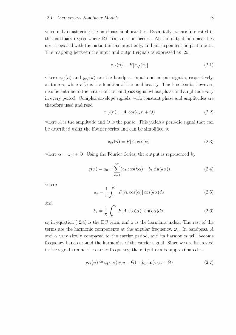
when only considering the bandpass nonlinearities. Essentially, we are interested inthe bandpass region where RF transmission occurs. All the output nonlinearitiesare associated with the instantaneous input only, and not dependent on past inputs.The mapping between the input and output signals is expressed as [26]
yrf (n) = F [xrf (n)] (2.1)
where xrf (n) and yrf (n) are the bandpass input and output signals, respectively,at time n, while F (.) is the function of the nonlinearity. The function is, however,insufficient due to the nature of the bandpass signal whose phase and amplitude varyin every period. Complex envelope signals, with constant phase and amplitudes aretherefore used and read
xrf (n) = A. cos(ωcn+Θ) (2.2)
where A is the amplitude and Θ is the phase. This yields a periodic signal that canbe described using the Fourier series and can be simplified to
yrf (n) = F [A. cos(α)] (2.3)
where α = ωct+Θ. Using the Fourier Series, the output is represented by
y(α) = a0 +∞∑k=1
(ak cos(kα) + bk sin(kα)) (2.4)
where
ak =1
π
∫ 2π
0
F [A. cos(α)] cos(kα)dα (2.5)
and
bk =1
π
∫ 2π
0
F [A. cos(α)] sin(kα)dα. (2.6)
a0 in equation ( 2.4) is the DC term, and k is the harmonic index. The rest of theterms are the harmonic components at the angular frequency, ωc. In bandpass, Aand α vary slowly compared to the carrier period, and its harmonics will becomefrequency bands around the harmonics of the carrier signal. Since we are interestedin the signal around the carrier frequency, the output can be approximated as
yrf (n) ∼= a1 cos(wcn+Θ) + b1 sin(wcn+Θ) (2.7)

2.1. Memoryless Nonlinear Models 9
where a1 and b1 are functions of A, Θ, and F . Incorporating A, Θ, and F in theequation, it can be rewritten as
yrf (n) = fA(A(n)) cos(ωcn+Θ(n) + fΘ(A(n))). (2.8)
Equations ( 2.1) and ( 2.8) in baseband exponential form are written as
x(n) = A(n)ejΘ(n) (2.9)
andy(n) = fA(A(n))e
j(Θ(n)+fΘ(A(n))) (2.10)
respectively. From equation( 2.10), fA(.) maps the input signal amplitude to theamplitude of the output, while fΘ(.) maps the baseband input amplitude to thephase of the output in the baseband representation. fA(.) and fΘ(.) are referredto as amplitude-to-amplitude (AM/AM) and amplitude-to-phase (AM/PM) map-ping/conversions respectively. The AM/AM and AM/PM distortions are importantcriteria in quantifying the performance of a PA based on the diversion from lineargain curve and phase shift, respectively [10].
Based on the AM/AM and AM/PM conversions, the PA memoryless nonlinear mod-els can be broadly categorized into two classes namely, strictly or quasi-memorylessmodels. Strictly memoryless models arise when the AM/PM is a constant, and inthis case, it does not vary with A(n) (usually in baseband transmission). Quasi-memoryless nonlinear amplifier models are obtained when the transmission is donein passband region, and hence both AM/AM and AM/PM conversions are not con-stant due to the introduction of both amplitude and phase distortions to the outputsignal. The power amplifier has short-term memory in this case since the signal timeinterval in memory is short compared to the period of signal envelope [27]. However,in baseband, PAs still exhibits memoryless input/output relationship.
2.1.1 Memoryless Polynomial Model
The model uses polynomial functions to fit the AM/AM and AM/PM mappings. Inbaseband representation, the PA is given by [28]
y(n) =P∑
p=0
c2p+1|x(n)|2px(n) (2.11)

2.1. Memoryless Nonlinear Models 10
where y(n) is the output signal, x(n) is the input signal in equation( 2.9) , andc2p+1 is the baseband coefficient of (2p + 1) nonlinear term. Only the odd-ordernonlinearity coefficients are in the baseband representation as even order termslie far from the passband and are easily filtered out. The AM/AM and AM/PMmappings are obtained from equation ( 2.11) and read
fA(A) =∣∣∣ P∑p=0
c2p+1|A(n)|2p+1∣∣ (2.12)
fΘ(A) = �( P∑
p=0
c2p+1|A(t)|2p+1). (2.13)
When the nonlinearity coefficients are real valued (in strictly memoryless case), theAM/PM conversion is zero, while complex valued coefficients yield non-zero AM/PMindicating quasi-memoryless nonlinearity.
The memoryless nonlinear model has been applied in predistorters for the develop-ment of nonlinear estimators and identification of wiener systems in [29] and [30],respectively.
2.1.2 Saleh Model
The model was proposed by A.A.M. Saleh in 1981 in [31] and was initially targetedfor modeling travelling-wave tube (TWT) amplifiers. The AM/AM and AM/PMmapping functions are,
fA(A) =αaA(n)
1 + βa(A(n))2(2.14)
fΘ(A) =αΘ(A(n))
2
1 + βΘ(A(n))2(2.15)
respectively, where αa, αΘ, βa, and βΘ are the four characteristic parameters ofAM/AM and AM/PM mappings. The model was further extended in the modelingof power amplifiers in general for both memoryless (frequency independent) andmemory-based (frequency dependent) applications. Among its application are incharacterization of PA nonlinearities in transmission systems [32], and design ofadaptive predistorters for high power PAs [33].

2.1. Memoryless Nonlinear Models 11
2.1.3 Ghorbani Model
The model was proposed in [34] as an advancement of the Saleh model to makeit applicable for modeling solid state power amplifier (SSPA). Unlike the TWTamplifiers, the SSPAs don’t have very large roll offs at saturation and the AM/PMmapping is much smaller. The AM/AM and AM/PM conversions are written as
fA(A) =α0(A(n))
α1
1 + α2(A(n))α1+ α3A(n) (2.16)
fΘ(A) =β0(A(n))
β1
1 + β2(A(n))β1+ β3A(n) (2.17)
where α0,α0, α0, α0, β0, β1, β2, and β3 are the model parameters in [34]. TheAM/AM mapping curve for small-signal amplification is in exponential form, whilethe AM/PM conversion has a logarithmic shape instead of linear curves as in theSaleh Model.
2.1.4 Rapp Model
The Rapp model takes a different approach in behavioral modeling by totally ne-glecting the AM/PM mapping [35]. It assumes the phase distortions are negligible,and hence in consequence in characterizing a PA. The AM/AM relationship is givenby
fA(A) =κA(n)(
1 +
(κA(n)
A0(n)
)2p)1/2p
(2.18)
where κ is the signal gain, A0(t) is the saturation amplitude at the output, p is thesmoothness parameter of the transition from linear to saturated state. The modelassumes a linear performance for small-signal input, whereas at high signal levels,the output begins to saturate approaching a constant value.
2.1.5 White Model
The model was proposed in [36] to accurately model SSPAs nonlinearities in theka-band (26GHz - 40GHz). It outperforms the Rapp, Ghorbani, and Saleh mod-els in nonlinearity modeling at high frequency bands. The AM/AM and AM/PM

2.2. Memory-Based Nonlinear Models 12
conversions are given by
fA(A) = a0(1− e−a1A) + a2Ae−a3A2
(2.19)
fΘ(A) =
⎧⎨⎩b0(1− e−b1(A−b2)), A ≥ b2
0, A < b2(2.20)
where a0 and a1 are the parameters representing the amplitude saturation leveland linear region gain, respectively, while a2 and a3 are used for matching thenonlinearity in the AM/AM conversion. The parameters b0, b1, and b2 are used tocontrol the magnification, the steepness, and the shift alongside the input amplitudeaxis, respectively.
2.2 Memory-Based Nonlinear Models
In the previous section, we discussed PA models that deal with frequency inde-pendent cases, where the input signal bandwidth is much less than bandwidth ofthe amplifier, and hence the frequency response of the PA is flat. However, whenwideband input signals are used for radio transmission, the PA exhibits frequency de-pendent behaviour and therefore a frequency selective response[18, 19, 24]. Besides,the PA nonlinearity cannot be purely defined by instantaneous mapping betweenthe input and output signals. In the real operating environment, the PA output isalso dependent on the previous input values due to delay caused by thermal andelectrical effects in the PA circuitry [37].
For accurate system-level simulations, the inclusion of the PA memory (dependenceon past inputs) in behavioral models becomes imperative to establish a comprehen-sive mapping between the PA input and output signals. Long term memory is usedto refer to the delay caused by thermal and memory effects. In the quasi-memorylesscase, the short-term memory was used to describe the phase distortion introducedby the use of complex-valued signals in passband transmission.
In this section, we will present the common models applied in literature to charac-terize the amplifier nonlinearity. We start with the Volterra series and its truncatedversions and finalize with the memory-based Saleh model.

2.2. Memory-Based Nonlinear Models 13
2.2.1 Volterra Series
The Volterra series presents the most extensive model for representing nonlinearsystems with memory, with the least amount of error. In the discrete time domain,it can be written as [38]
yrf (n) = w0
+∞∑
τ1=0
w1(τ)xrf (n− τ1)
+∞∑
τ1=0
∞∑τ2=0
w2(τ1, τ2)xrf (n− τ1)xrf (n− τ2)
+ ...
+∞∑
τ1=0
∞∑τ2=0
...∞∑
τp=0
wp(τ1, τ2, ...τp)xrf (n− τ1)xrf (n− τ2)...xrf (n− τp)
(2.21)
where yrf (n) and xrf (n) are the input and output signals in the passband region,respectively. The functions w0 w1(τ), w2(τ1, τ2), and wp(τ1, τ2, ...τp) are the Volterrakernels (the model parameters). They represent the nonlinearity orders of the sys-tem. For instance, w0 is the zeroth-order kernel (the DC term), and w1 is the 1storder kernel (linear filter), and the rest are higher order convolutions. The blockdiagram in Figure 2.1 illustrates the Volterra series. The series is written more
Figure 2.1 A simple block diagram illustrating the Volterra model in [20].

2.2. Memory-Based Nonlinear Models 14
compactly and simplified as [39]
yrf (n) =∞∑p=1
∞∑τ1=0
· · ·∞∑
τp=0
hp(τ1, · · · , τp)Dp(xrf (n)) (2.22)
where hp(τ1, · · · , τp) are the Volterra model parameters, and
Dp(xrf (n)) =P∏
p=1
xrf (n− τp) (2.23)
where Dp(.) is the pth-order Volterra operator. The Volterra series in the aboveequations is very complicated, especially when a large number of parameters arerequired to represent high degree of nonlinearity and memory depth. This increasesthe complexity in the identification of parameters and number of convolutions dur-ing system level simulation. Therefore, it becomes very complex to use it in theabove forms. To mitigate the model complexity and improve its performance, sev-eral approaches have been devised, which include pruning and dynamic reductiontechniques.
The dynamic deviation reduction (DDR)-based Volterra series was proposed in [40],and involves the separation and control of Volterra coefficients from different dy-namic orders. The model is shown to reduce complexity without compromising thesystem performance, by using a very small number of parameter to represent bothnonlinearity and memory depth. The model’s number of parameters increase almostlinearly with the nonlinearity order and memory depth, unlike in classical Volterraseries where the number of coefficients increase exponentially.
The DDR-based Volterra series is written as
yrf (n) =P∑
p=1
hp,0(0, . . . , 0)xprf (n)
+P∑
p=1
{p∑
r=1
[xp−rrf (n)
M∑τ1=1
. . .M∑
τr=τr−1
·hp,r(0, . . . , 0, τ1, . . . , τr)r∏
j=1
xrf (n−τj)
]}(2.24)
where P and M denote the order of nonlinearity and memory length respectively.During the regrouping of the parameters based on the order of dynamics, the variable

2.2. Memory-Based Nonlinear Models 15
r is used to represents the dynamics. hp,r(0, . . . , 0, τ1, . . . , τr) is the Volterra kernelwith rth-order dynamics and pth-order nonlinearity. The variable r can be adjustedfurther in real PAs to remove high order dynamics whose effects are insignificantin-terms of contribution to overall nonlinear dynamics.
The classical and DDR-based Volterra series described above use polynomial-typefunctions, which require wide observation bandwidth when wide bandwidth is em-ployed for radio propagation or when the PA has high order nonlinearity. A ban-dlimited version of the Volterra series is presented in [20]. It is accomplished bycontrolling the bandwidth of the Volterra operators using a bandlimiting functionbefore being multiplied by their respective coefficients. The Volterra operator inequation ( 2.23) is modified by inserting a bandlimiting function f(.) in time do-main to yield
Tp(xrf (n)) = Dp(xrf (n))⊗ f(n) (2.25)
where ⊗ denotes the convolution operation between the bandlimiting function f(n)
and classical Volterra operator. After the modification, the bandlimited classicalVolterra series is written as
yrf (n) =∞∑p=1
∞∑τ1=0
· · ·∞∑
τp=0
hp,BL(τ1, · · · , τp)Tp(xrf (n))
=∞∑p=1
∞∑τ1=0
· · ·∞∑
τp=0
hp,BL(τ1, · · · , ip)(Dp(xrf (n))⊗ f(n))
(2.26)
where f(n) is the bandlimiting function with length M , hp,BL(τ1, · · · , τp) is thepth order bandlimited Volterra model parameters. The output y(n) is logicallybandlimited since all the Volterra operators are bandlimited, leading to completebandlimited system, as shown in Figure 2.2. The same modeling operations areapplied on a 1-st order DDR-based Volterra series and it results in a bandlimitedmodel. In the expanded form, it can be written as [20]
yenv(n) =
(P−1)/2∑p=0
M∑τ=0
g2p+1,1(τ)
[N∑
m=0
|xenv(n−m)|2pxenv(n− τ −m)fenv(m)
]
+
(P−1)/2∑p=1
M∑τ=1
g2p+1,2(i)
[N∑
m=0
|xenv(n−m)|2(p−1)x2env(n−m)x∗
env(n− τ −m)fenv(m)
](2.27)
where the P and M are the nonlinearity order and memory length, respectively.

2.2. Memory-Based Nonlinear Models 16
Figure 2.2 An Illustration of the band-limited Volterra model in [20]. The Volterrakernels are bandlimited before multiplication with their respective coefficients
xenv(n) and yenv(n) denote the complex envelopes of the input and output, re-spectively, at baseband, while g2+1,j(.) is the complex bandlimited Volterra modelparameters.
2.2.2 Memory Polynomial Model
The memory polynomial model is a truncated version of the Volterra series thatincludes only the diagonal elements [41]. The model is also called the parallel Ham-merstein (PH) model. It is widely used for modeling of PAs exhibiting memoryeffects. The baseband output waveform is given by
y(n) =M∑j=0
N∑i=1
aji · x(n− j) · |x(n− j)|i−1 (2.28)
where aji are the model coefficients while N and M are the nonlinearity order andmemory depth, respectively.
There are other variants of the model which have been proposed. One of the widelyapplied model is the generalized memory polynomial (GMP) model. The modelconstruction involves merging of the memory polynomial model with the cross termsbetween the signal and the lagging/leading envelope terms. The generalization of the

2.2. Memory-Based Nonlinear Models 17
memory polynomial enables the inclusion of the memory effects caused by transportdelays and rapid thermal changes in active devices which affect the signal waveform.The incorporation of these imperfections improve the linearization performance ofthe model compared to the memory polynomial [42]. The model can be written as
yGMP(n) =Ka−1∑k=0
La−1∑l=0
aklx(n− l) |x(n− l)|k
+
Kb∑k=1
Lb−1∑l=0
Mb∑m=1
bklmx(n− l) |x(n− l −m)|k
+Kc∑k=1
Lc−1∑l=0
Mc∑m=1
cklmx(n− l) |x(n− l +m)|k .
(2.29)
where KaLa, KcLcMc, and KbLbMb represent the number of coefficients for alignedsignal and envelope (which is the case of the memory polynomial), coefficients forsignal and leading envelope, and coefficients for signal and lagging envelopes, re-spectively. The memory polynomial structure is a special case of the model whereonly the aligned signal and envelope terms are included.
2.2.3 Wiener Model
The Wiener model is a two-box model that is a cascade of a linear dynamic block(FIR or IIR filter) followed a memoryless nonlinearity (usually a polynomial-typefunction) as shown in figure 2.3. The model input and output signals can be given
𝑥(𝑛) 𝑦(𝑛)𝑢(𝑛) 𝐹(. )𝛽(𝑛)Amplifier
Figure 2.3 A block diagram of the Wiener model, which is a cascade of a linear dynamicblock followed by a memoryless nonlinearity.
as
u(n) =M∑τ=0
βτx(n− τ) (2.30)

2.2. Memory-Based Nonlinear Models 18
andy(n) = F (u(n)) (2.31)
where F (.) is the memoryless nonlinearity, and βτ (k) is the linear dynamic block. Ascan be seen from equation ( 2.30), the modeling methodology flouts the identificationprocedures used in identification of nonlinear systems, hence, it becomes difficult towrite the output y(n) explicitly as a function of x(n). This leads to difficulties inparameter estimation and inversion of the equation during linearization.
The linear filter used in the dynamic block is only able to correct electrical memorycaused by frequency response of the amplifier. However, it is not sufficient to esti-mate the impedance disparities due to harmonic loading and bias circuits. As such,another higher order filter is added downstream the wiener model, and system iscalled the augmented Wiener model [24]. The equation ( 2.30) now becomes,
u(n) =M∑τ=0
βτx(n− τ) +M∑τ=0
βτx(n− τ)|x(n− τ)| (2.32)
with equation ( 2.31) remaining the same.
2.2.4 Hammerstein Model
The Hammerstein model is also a two-box model that is a cascade of a static mem-oryless nonlinearity followed by a dynamic linear block (IIR or FIR filter). It issimilar to the Wiener model with the order of the two blocks reversed as shown inFigure 2.4. The nonlinear static block can written as
𝑥(𝑛) 𝑦(𝑛)𝑢(𝑛)𝐹(. ) 𝛽(𝑛)Amplifier
Figure 2.4 A block diagram of the Hammerstein model, which is a cascade of memorylessnonlinearity and a linear dynamic block.

2.2. Memory-Based Nonlinear Models 19
u(n) = F (x(n)) (2.33)
where F (.) is the nonlinear block (usually a polynomial-type function) and x(n) isthe input signal. The system output can then be written as
y(n) =
M1∑τ=0
βτu(n− τ)
=
M1∑τ=0
βτF (x(n− τ)).
(2.34)
The concept of the augmented Wiener model is extended to the Hammerstein modelgiving rise to a dual, the augmented Hammerstein model. As such, another highorder filter is added upstream the Hammerstein model. This yields an expressionthat reads
y(n) =
M1∑τ=0
βτF1(x(n− τ)) +
M2∑τ=0
βτF2(x(n− τ))|x(n− τ)| (2.35)
where F1(.) and F2(.) are the nonlinear mappings of the first and second filters, re-spectively. M1 and M2 represent the memory depth of the first and second equations,respectively.
2.2.5 Wiener - Hammerstein Model
The two models are combined together, to form a generalized model, consistingof a linear dynamic block, followed by memoryless polynomial type function andanother linear dynamic block. When a signal is inputted, it is first pre-filtered,then nonlinearity is applied, and finally post-filtered to obtain the final output, asillustrated in Figure 2.5. Therefore, there are two intermediate signals, u1(n) andu2(n), whose baseband equivalent forms can be written as,
u1(n) =
M1∑τ=0
βτx(n− τ) (2.36)
u2(n) = F (u1(n)). (2.37)

2.3. Discussion 20
𝐹(. )𝑢 (𝑛) 𝑢 (𝑛)𝑥(𝑛) 𝑦(𝑛)𝛽(𝑛) 𝛾(𝑛)Figure 2.5 A block diagram of the Wiener-Hammerstein model.
The final equation, with x(n) as input signal, can now be written as,
y(n) =
M1∑i=0
γiu2(n− i)
=
M1∑i=0
γiF (u1(n− i))
(2.38)
2.2.6 Saleh Memory-Based Model
This is the frequency dependent version of the Saleh model, and is used on frequencyselective channels (this is usually the case when wideband input signals are appliedon the PA). The parameters αa, αΘ, βa, and βΘ in equation( 2.14) become frequencyselective, and the input/output in-phase and quadrature signal conversions now read,
SI(A,w) =αa(f)A
1 + βa(f)A2(2.39)
SQ(A,w) =αb(f)A
3
(1 + βb(f)A2)2(2.40)
where S1 and SQ are the in-phase and quadrature signal mappings, respectively.
2.3 Discussion
In this chapter, both the memoryless and memory-based PA models have been dis-cussed, with emphasis put on the formulation and representation of PA nonlinearityin equations and block diagrams. The memoryless models have less parameters and

2.3. Discussion 21
are easy to identify and formulate. However, they may not accurately represent theperformance of the PA since they don’t factor in crucial non-idealities in the realoperating environment. Moreover, wideband power amplifiers exhibit frequency de-pendent behavior and therefore frequency selective response. Memory-based PAmodels are adopted in most simulation-level environments because they don’t onlyrepresent the frequency selective behavior but also memory and electrical effects,which may cause significant influence of the PA model parameters.
In the discussions, however, the issue of identification complexity has not been dealtwith comprehensively. The detailed analysis of the models’ identification complexityin FLOPS has been in done[17], with the corresponding linearization performanceon different commercial PAs being reported also. For instance, the GMP model wasshown to have the highest accuracy vs. FLOPS at the lowest computational costfollowed by the PH model when evaluated using the widely used Doherty amplifier.The Volterra series offers the best performance in all the PA scenarios when thecomplexity perspective is not considered.

22
3. EFFECTS AND MITIGATION OF POWER
AMPLIFIERS NONLINEARITY
Power amplifiers are inherently nonlinear, and therefore negatively affect the perfor-mance of the entire analog front-end by causing RF impairments. The alleviation ofthe PA nonlinearity is essential in preserving the integrity of the information in thetransmitted signal and reducing the interference and cross-talk with the adjacentchannels. These adverse effects include inband distortion, adjacent band interfer-ence, and distortion of the signal envelope in QAM modulation scheme. The en-hancement of PA linearity enables the use of very dense signal constellations, whichtranslates to higher spectral efficiency. Moreover, PA power efficiency is highlydesirable to achieve maximum coverage when the operation is near the saturationregion.
In this chapter, we will start by analyzing the effects of the power amplifier nonlin-earity on single tone and multitone communication signals. In particular, the effectsof harmonic and intermodulation (IMD) components on the PA input signal charac-teristics will be presented. In the other sections, the widely used analog and digitallinearization methods are explored, with emphasis put on digital predistortion.
3.1 Effects of Power Amplifier Nonlinearity
The PA has a nonlinear profile, hence it distorts the input signal by introducingunwanted emissions in the inband (in the occupied transmit band), out of band(OOB), and spurious regions. The OOB emissions are in the adjacent bands nextto the main carrier, and are defined in terms of the ACLR and spectral mask [1].The spurious emissions occupy other parts more far away in the spectrum and arealso caused by harmonic and intermodulation products.
In this analysis, we use a two-tone signal to demonstrate the introduction of un-wanted emissions by a PA using a third order memoryless polynomial-type nonlinear

3.1. Effects of Power Amplifier Nonlinearity 23
system. The nonlinear system is given by
y = a.xin + b.x2in + c.x3
in (3.1)
where y and xin are the output and input signals, respectively, while a, b, and c arethe system nonlinear coefficients. The input signal xin is a two-tone signal given by
xin(t) = A1. cos(w1t) + A2. cos(w2t) (3.2)
where A1 and A2 magnitudes of the two signals, and w1 and w2 are the angularfrequencies of the two signals with w2 > w1.
By combining equations ( 3.1) and ( 3.2), the output signal becomes [43]:
y =
[1
2bA2
1 +1
2bA2
2
]︸ ︷︷ ︸
DC component
+
[(a+
3
4cA2
1 +3
4cA2
2
).A1. cos(w1t) +
(a+
3
4cA2
2 +3
4cA2
1
).A2. cos(w2t)
]︸ ︷︷ ︸
amplified fundamental frequencies(wanted signal)
+
[1
2bA2
1 cos(2w1t) +1
2bA2
2 cos(2w2t)
]︸ ︷︷ ︸
second order harmonics
+
[1
4cA3
1 cos(3w1t) +1
4cA3
2 cos(3w2t)
]︸ ︷︷ ︸
third order harmonics
+ [bA1A2 cos((w2 − w1)t) + bA1A2 cos((w2 + w1)t)]︸ ︷︷ ︸second order IMDs
+
[3
4cA2
1A2 cos((2w1 − w2)t) +3
4cA1A
22 cos((2w2 − w1)t)
]︸ ︷︷ ︸
in-band third order IMDs
+
[3
4cA2
1A2 cos((2w1 + w2)t) +3
4cA1A
22 cos((2w2 + w1)t)
]︸ ︷︷ ︸
OOB third order IMDs
.
(3.3)From equation ( 3.3) and as illustrated in Figure 3.1, it is clear that there are un-wanted emissions (frequency components) that have been introduced to the outputsignal. The resultant frequency components can be broadly classified into threegroups [43]:
• The useful/wanted signal. This is the linearly amplified signal comprising ofthe fundamental frequency components, w1 and w2.

3.1. Effects of Power Amplifier Nonlinearity 24
• Unwanted signals removable by filtering. In addition to the useful signal, thereare other frequency components, i.e DC component, second order harmonicsand intermodulation products (IMDs), and third order harmonics and OOBIMDs, which fall in the spurious domain. They are far from the fundamentalfrequencies and are easily removed by RF filtering.
• Unwanted signals that are not removable by filtering. These are the signalcomponents that fall directly on top or in the immediate vicinity of the mainfrequency components. It is infeasible to filter out these components since itrequires a high order filter, which increases the processing complexity.
Figure 3.1 Frequency domain output of a third-order nonlinear system driven by two-toned signal.
The above analysis can be extended to predict the nonlinear behavior of multi-tonesignals such as OFDM signals where many sub-carriers are closely spaced, and incontinuous spectrum signals. This is illustrated in Figure 3.2, and shows the spectralregrowth which falls both on the spurious and OOB domains.
The PA nonlinearity is detrimental in modern communication systems which em-ploy high order complex modulation schemes (e.g. 64 QAM and 256 QAM) andadvanced multiplexing schemes (e.g. OFDM). The resultant transmit signals havehigh envelope fluctuations which falls in the nonlinear region of the amplifier. Thehigh signal variations are characterized by the PAPR, calculated as
PAPRdB = 10 log
(Pmax
Pavg
)(3.4)
where Pmax and Pavg are the signal’s peak and average power levels, respectively. Theoperating PAPR of most communication systems is 10 - 13 dB, and therefore there

3.2. Feedback Linearization 25
f
Spuriousdomain
Spuriousdomain
ChannelBandwidth
OOBregion
OOBregion
subcarriersUnwanted EmissionsUnwanted Emissions
Figure 3.2 Transmitter spectrum of a multicarrier signal. The PA output contains spec-tral regrowth and occupies both the spurious and OOB domains.
is need to lower the high envelope fluctuations to achieve the linear amplification.Different methods of lowering the PAPR have been proposed in [44, 45, 46]. Thepower amplifier efficiency is jointly improved by slightly reducing the PAPR andusing a PA linearization scheme, which ensures the PA operates near the saturationpoint and the gain expansion capabilities of the linearization scheme are leveraged.In the next section, the different approaches employed for linearization are discussed.
3.2 Feedback Linearization
Feedback linearization is one of the simplest method of mitigation of PA nonlinearityand uses a feedback loop for error cancellation. The principle of operation is toextract the error signal from the output signal by comparing it with the inputsignal, and then injecting it back to the PA with opposite phase [47]. The methodis widely used for amplification of narrowband signals, such as in audio amplifiers.A basic feedback system is shown in Figure 3.3. It has a comparator for calculatingthe error signal from the input signal and the signal from the feedback path. Thefeedback system is able to compensate the error signal when the bandwidth involvedis small (in kHz range), however, error cancellation becomes problematic when thesignal bandwidths are wide.
Several methods have therefore been proposed to overcome this challenge. Theyinclude the Cartesian modulation feedback, and envelope feedback, among others.

3.2. Feedback Linearization 26
Figure 3.3 A basic structure of a feedback system.
The Cartesian feedback involve two loops, one for the in-phase component and otherfor the quadrature component. The feedback signal is down-converted to basebandand the error computation is done separately for the I and Q components. Theprocessing of the signals at baseband eliminates the delay synchronization problemsbecause of the slow variations of the baseband equivalent signal.
In the envelope feedback in [48], only the envelope of the signal is detected and cor-rected. Envelope detectors are employed at the feedback loop and signal generator,and a comparison of the two signals is done. The resultant signal is then fed toa gain controller via a low pass filter. Figure 3.4 shows a basic envelope feedbacksystem, where an envelope generator and detector are used for mitigation of PAnonlinearity for an I/Q signal source.
I/Q signal generator RF Modulator
Envelope Detector
Gain Control
Envelope Generator
PA
LowpassFilter
-
Output
Figure 3.4 A simplified structure of an envelope feedback system.

3.3. Feedforward Linearization 27
3.3 Feedforward Linearization
The linearization is done by obtaining the output signal of the amplifier and iden-tifying the distortions in the signal, and then doing the distortion cancellation afterthe PA. A typical circuit of a feedforward linearizer is shown in the Figure 3.5.This involves the implementation of two loops, one for signal cancellation (SCL)and the other for error cancellation (ECL). The SCL is used for identification of
VectorAttenuator
VectorAttenuator
Delay element
Delay element
ErrorAmplifier
Main PA
Signal Cancellation Error Cancellation𝑥(𝑡)𝑐
𝑦(𝑡)𝑐𝐿
𝑐
𝑐𝑧(𝑡)
Figure 3.5 A block diagram of a feedforward linearization system and its essential com-ponents.
the distortions caused by the PA. The input signal is separated by a coupler C1
into two branches, an upper branch where signal is fed to the PA, and a lowerbranch where the signal goes through a delay circuit before been coupled with anattenuated output signal from the PA. The attenuator Lc and the delay elementensure that the signals at the inputs of the coupler C3 have same power level andare synchronized, respectively. The coupler C3 yields an error signal e(t) which isthe difference between the synchronized output and the input signals, and containsthe signal distortion caused by the PA.
The error signal e(t) and the coupled output signal are then fed to the ECL loop,which does the cancellation of the error signal. The error signal e(t) is passedthrough a vector attenuator for scaling and phase tuning before been amplified to

3.4. LINC 28
the power level of the signal in the upper branch. The amplification is necessaryto ensure both upper and lower branches have the same power level for effectivecancellation. The upper and lower branches signals are injected to the coupler C4
which cancels the error and yields a distortionless signal z(t).
However, the whole cancellation system is suspectible to variation in operating condi-tions and coefficient mismatch in the ECL and SCL loops when adaptive algorithmsare applied. Besides, phase and gain matching between all the circuit elements mustbe maintained at high accuracy for the error cancellation to be effective [49].
3.4 LINC
LINC is an acronym for linear amplification with nonlinear components. The methodinvolves the splitting of the signal into two constant envelope signals whose sumyields the original signal [50]. The two signals are then passed separately throughnormal power amplifiers and their outputs combined to form the transmit signal.The transmit signal is free from any nonlinearity since the AM/AM and AM/PMmappings are flat due to the linear amplification of the constant envelope signals.Harmonic components originating from the nonlinear amplifiers are easily suppressedby a low pass filter. The LINC system is illustrated in Figure 3.6.
Figure 3.6 A simplified Linearization structure using the LINC Concept.
A general baseband equivalent signal flow through the LINC system is analyzed

3.5. CALLUM 29
below. A baseband signal can written as,
s(t) = A(t). cos(wt+ φ(t)) (3.5)
The two constant envelope signals are derived from equation ( 3.5) and are writtenas,
s1(t) =amax
2. cos(wt+ α(t)) (3.6)
s2(t) =amax
2. cos(wt− α(t)) (3.7)
where amax is maximum amplitude of A(t). To obtain a linearly amplified version ofthe original signal from the sum of the two equations, the phase of the signals α(t)
should be defined as,
α(t) = cos−1
(A(t)
amax
)(3.8)
The LINC method suffers from a major drawback in power combining after thePAs due to difficulties in component separation, and subsequent synchronizationand combining of the two signals after amplification. When the two signal areuncorrelated, the combining results in a 3 dB insertion loss which degrades theperformance of the entire system [51].
3.5 CALLUM
CALLUM is the abbreviation for combined analogue locked loop universal modula-tor. It uses same operating principle as the LINC system but the constant envelopesignals are generated by combining the I and Q components of the input signalseparately with signals obtained from a feedback loop [52]. The feedback receiversignal is demodulated and each of the I/Q components is compared with the re-spective input components to form the error signals. The error signals are fed to avoltage controlled oscillator (VCO) and then to the PA, producing a high gain loop.The phase and gain of the transmitter are precisely controlled by the feedback loopensuring the error signal is minimized. Figure 3.7 shows a basic CALLUM structure.
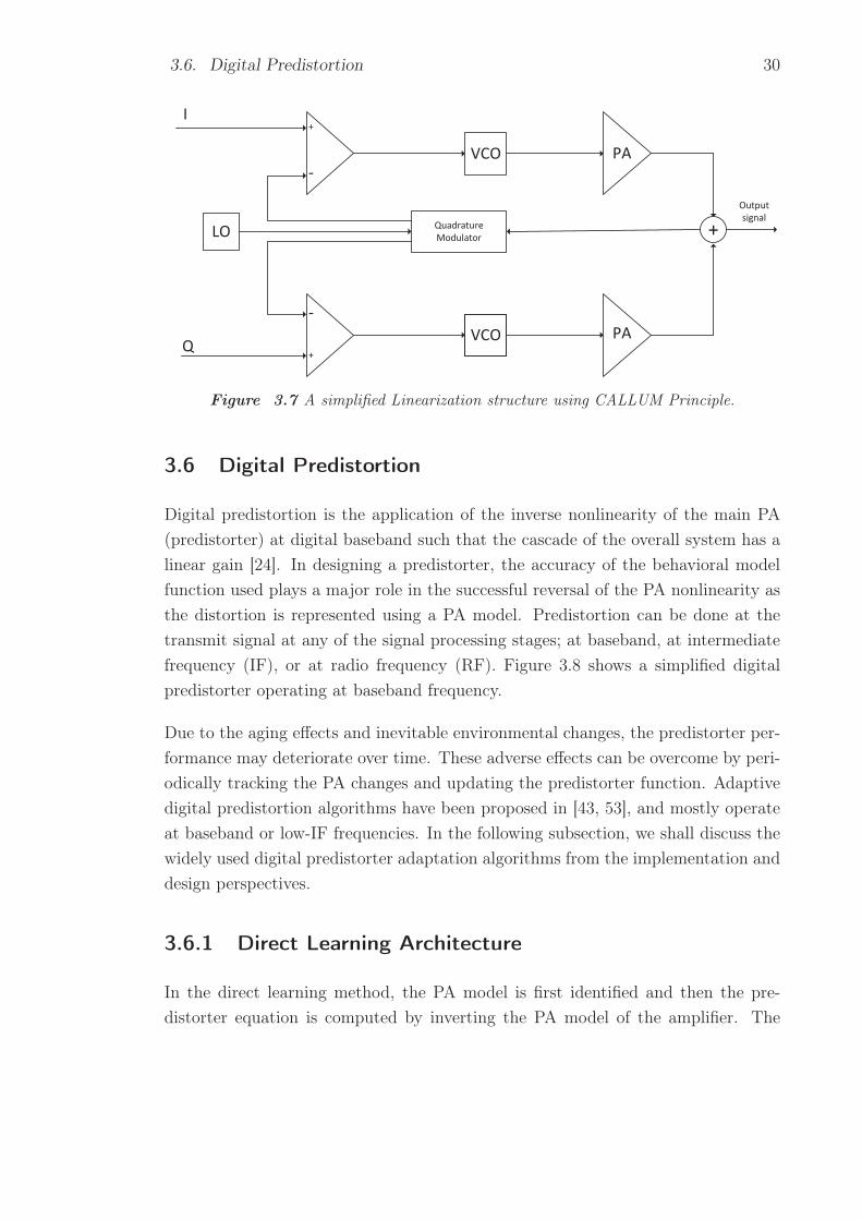
3.6. Digital Predistortion 30
VCO
QuadratureModulatorLO +
I
Q VCO
+
-
+
PA
PA
-
Outputsignal
Figure 3.7 A simplified Linearization structure using CALLUM Principle.
3.6 Digital Predistortion
Digital predistortion is the application of the inverse nonlinearity of the main PA(predistorter) at digital baseband such that the cascade of the overall system has alinear gain [24]. In designing a predistorter, the accuracy of the behavioral modelfunction used plays a major role in the successful reversal of the PA nonlinearity asthe distortion is represented using a PA model. Predistortion can be done at thetransmit signal at any of the signal processing stages; at baseband, at intermediatefrequency (IF), or at radio frequency (RF). Figure 3.8 shows a simplified digitalpredistorter operating at baseband frequency.
Due to the aging effects and inevitable environmental changes, the predistorter per-formance may deteriorate over time. These adverse effects can be overcome by peri-odically tracking the PA changes and updating the predistorter function. Adaptivedigital predistortion algorithms have been proposed in [43, 53], and mostly operateat baseband or low-IF frequencies. In the following subsection, we shall discuss thewidely used digital predistorter adaptation algorithms from the implementation anddesign perspectives.
3.6.1 Direct Learning Architecture
In the direct learning method, the PA model is first identified and then the pre-distorter equation is computed by inverting the PA model of the amplifier. The

3.6. Digital Predistortion 31
Figure 3.8 A functional block diagram of Baseband DPD Linearization system and corre-sponding gain characteristics of predistorter and PA. The gain expansion at the predistortercompensates the gain compression exhibited by the PA resulting in a linearized RF output.
predistorter is updated with the computed inverse equation. The method is easilyapplicable to memoryless PA models/systems where the instantaneous input andoutput AM/AM and AM/PM mappings exist. In memory-based PA models andsystems, the PA function inversion becomes much more complicated [54]. Figure3.9 illustrates a direct learning architecture, where PA model is computed beforeinversion is done.
Predistorter
Model InversionPA Model
G1
+-
PA
PA InDPD In PA Out
CoefficientUpdate
Figure 3.9 Direct learning Architecture.

3.6. Digital Predistortion 32
3.6.2 Indirect Learning Architecture
The indirect learning algorithm is developed to ease off the complication and errorsexperienced in the DPD function inversion. The post-inverse of the PA is first iden-tified by interchanging the input and the output signals, and the resultant functionis used as the predistorter function upstream.
Predistorter
Post-Inverse
G1
+ -
PADPD In PA Out
CoefficientUpdate
PA In
Figure 3.10 Indirect learning Architecture.
However, the system suffers from reduced power range due to the interchanging ofthe input and output during calculation of the post-inverse. This limits the operationof the amplifier up to a particular input power level below the saturation point.
3.6.3 Closed Loop Adaptive Digital Predistortion
The predistorter is inside the feedback adaptation loop that is used for parameterupdate. Figure 3.11 illustrates the closed loop block diagram, where the input andoutput signals of the PA are used to calculate the error signal, which is used by theadaptive algorithm to update the parameters to be fed to the predistorter. In thismethod, the distortion signal is minimized in subsequent loops until convergence isachieved. Furthermore, the closed loop estimation and update is less sensitive tonoisy feedback observations compared to the direct and indirect learning architec-tures discussed in the previous sections [55].
In Chapter 4, the closed loop decorrelation-based method is used for parameterlearning.

3.7. Discussion 33
Predistorter
AdaptiveAlgorithm
G1
+ -
PAPA InDPD In PA Out
CoefficientUpdate
ErrorSignal
Figure 3.11 Closed Loop Adaptive learning Architecture.
3.7 Discussion
PAs are nonlinear devices that cause significant RF imperfections on the transmitsignal. Among the negative effects of the nonlinear behavior of the PA are distortionof the signal envelope, adjacent channel interference, and the introduction of inbandwaveform impurities. The introduction of the nonlinear distortions by the PA hasbeen exemplified using a two-tone signal applied to a third order nonlinear system.The unwanted frequency components introduced can be classified into three groupsnamely; inband distortion, OOB distortion, and spurious emissions.
The spurious emissions are more far in the spectrum from the input signal and can besuppressed using the transmit or cavity filters, while inband and OOB emissions re-quire the use of alternative methods for cancellation. The alternative methods devel-oped include the feedback linearization, feedforward linearization, LINC, CALLUM,and digital predistortion, among others. The above methods cancel the PA nonlin-earity significantly when operated near saturation (with minimum power back-off),hence enhancing power efficiency. This effectively allows the use of high-order denseconstellations, thus improving spectral efficiency. The above methods, however, havetheir shortcomings in terms of the complexity, adaptation to environmental changes,linearization performance, and applicability in modern communication systems. Inthis light, the selected linearization method should provide the best tradeoff among

3.7. Discussion 34
the above competing interests in a communication system.

35
4. BANDLIMITED DIGITAL PREDISTORTION
In this chapter, we introduce and analyze the concept of bandlimited predistortionin continuous transmit spectrum or contiguous CA of two or more CCs. In bothmobile handsets and base station transmitters, the need to linearize the inbandand adjacent spectral distortions caused by the nonlinear amplifiers is becomingextremely important due to the increasing bandwidth allocations of the transmitsignal to accommodate higher data rates while still ensuring power efficiency [1].This has, however, become strenuous to the entire transmitter chains due to theincreasing number of computations and high speed converters required for signalprocessing. For instance, there is an increase in the sample rates required for ADCand nonlinearity observation in the feedback receiver. The increased complexity insystem design may make DPD linearization infeasible for wide bandwidth allocationsproposed for future LTE-A implementations.
For wide bandwidth allocations, the suppression of inband distortion and spectralregrowth can be done in two ways: First, the inband distortion and spectral regrowthin the very near vicinity of the transmit band can be linearized using DPD, and thespectral regrowth more far from the main carrier(s) are filtered out using a bandpassfilters at the PA output or cavity filters in duplexers of FDD transceivers. Theproposed approach yields the following benefits [56]:
• There is a significant reduction in the bandwidth required for PA feedbackobservation, in that only a fraction of the PA nonlinearity is observed forlinearization using DPD. This consequently reduces the sample rate of theADC in the feedback path.
• The bandlimited DPD solution offers an extra degree of freedom in the lin-earization of PA nonlinearity. The extent of the bandwidth to be linearized canbe chosen using a bandlimiting function based on the nonlinearity suppressionneeded and the nonlinearity profile of a PA. This is particularly simple sincethe bandlimiting filtering is done in the discrete-time domain.

4.1. Basics of Sampling and Filtering Theory 36
• The filtered basis functions used in the proposed DPD solution are gener-ated using lower sample rates and computational cost compared normal basisfunctions in conventional DPD methods.
We start by analyzing the signal processing of baseband equivalent signal and theeffects of sample rates used in DPD processing in mitigating the PA nonlinearity.Thereafter, we develop a distortion component model where we formulate the PAnonlinearity and the SNL basis functions to be used for DPD learning and parameterupdate. We finalize the chapter by analyzing the parameter update algorithmsemployed namely, the sample and block closed-loop decorrelation-based learning.
4.1 Basics of Sampling and Filtering Theory
In digital communication systems, signal generation is done in time domain andthen digitally modulated into in-phase and quadrature (I/Q) components for RFtransmission. Modern radio systems use the direct-conversion transceiver archi-tecture which involves the use of complex I/Q signal processing for baseband toRF frequency conversion. The frequency translation is done by multiplying thesignal with a complex-valued signal from a numerically-controlled oscillator whosefrequency is the centre frequency of the allocated channel band in spectrum.
The input signal is resampled to a higher sampling rate depending the transmissionand predistortion requirements of the system. For instance, for LTE-A signal witha bandwidth of 20 MHz, the signal generation is done at 30.72 mega-samples persecond (MSa/s) and then upsampled by 4 or 5 times to yield a DPD sample rateof 122.88 MSa/s or 153.6 MSa/s, respectively, to accommodate the PA nonlinearityand predistorter observation path [1]. However, the required five time over samplingrate may not be sufficient to capture all the PA nonlinearity when the PA is drivennear saturation. Operating the PA near saturation requires that a higher orderbehavioral model is adopted, usually a 11th- or 13th- degree nonlinearity, to obtainall significant spectral distortions [53]. Otherwise, the simulation results may notbe valid when real PA implementations are done.
The upsampling of the I/Q signals is performed to increase the sample rates sincethe predistorter increases the bandwidth requirement of the PA input signal to en-sure linearization occurs in the adjacent bands. In case the expanded bandwidth isless than the PA nonlinearity profile, aliasing is bound to occurs to the side-bands

4.1. Basics of Sampling and Filtering Theory 37
of the PA output signal, and therefore the feedback observation receiver signal willbe corrupted, affecting the overall performance of the predistorter. Likewise, under-sampling will also have the same effect on the linearization performance, making itimpossible to recover the transmitted signal by resampling at the PA output. Hence,the sample rates adopted should accommodate the PA nonlinearity profile as wellas the DPD bandwidth requirements. Figure 4.1 shows the effects of undersamplingand oversampling.
Figure 4.1 The effects on sampling rates of the DPD signal. The predistorted signal (b)has a wider bandwidth than the original signal (a). Low sampling rates leads to under-sampling in (c) resulting in aliasing of the side-bands, hence the original signal cannot berecovered thereafter. Oversampling prevents aliasing as is the case in (d).
The sample rates required to accommodate high degree nonlinearity are usually veryhigh especially when the signal is transmitted using wide bandwidths. In scenarioswhere high data rates are highly desirable and necessary, the deployment of one ormore component carriers (CCs) with a resultant bandwidth of more than 20 MHzwould require very wide channel bands to capture the entire nonlinearity profile forhighly nonlinear amplifiers. This would increase sample rates to exhobitant levels,and further escalate the hardware requirements for the DACs and ADCs.
The above implementation problem can be mitigated by using the bandlimited con-

4.1. Basics of Sampling and Filtering Theory 38
cept introduced in [20] and [21] by limiting the band to be linearized using a ban-dlimiting function. A bandlimited Volterra-series is proposed in [20] (explained insubsection 2.2.1) to limit the expansion of the bandwidth during behavioral model-ing by bandlimiting the input and output signals. This is later applied in [21] forDPD linearization of different implementation scenarios for contiguous and noncon-tiguous CA of two or more CCs allocations. The performance of the these systemsis evaluated and excellent suppression of the inband distortions and OOB (in thelinearized bandwidth) distortions is reported in all the scenarios. In this thesis, weextend the bandlimiting concept by introducing a filtering function to reduce theDPD running bandwidth (i.e., by bandlimiting the bandwidth of the PA feedbackobservation signal and the basis functions bandwidth), thereby preventing aliasingfrom occurring when lower sample rates are employed, as depicted in Figure 4.2.
Figure 4.2 The effect of bandlimiting the DPD output on the sampling rate. Bandlimitingreduces the bandwidth occupied by the predistorter signal and hence lower sampling ratescan be employed without aliasing occuring.
In the implementations, the computational cost of the bandlimiting functions isnot evaluated, and the subsequent effect on the inband and OOB suppression isalso not analyzed. A tradeoff between the computational cost of multiplying theinput and output signals with bandlimiting function(s) and the DPD suppressionperformance is inevitable. The higher the order of the bandlimiting functions, thehigher the nonlinearity suppression. However, there is a resultant increase in thecomputational cost of doing the filtering. The quantitative performance tradeoff isanalyzed through simulations and RF measurements in Chapter 5.

4.2. Digital Predistortion Modeling 39
4.2 Digital Predistortion Modeling
In this section, practical cases of a single CC or contiguous CA of two or moreCCs is assumed for the signal modeling. The input signal to the PA and will bedenoted by x(n) in both scenarios for simplicity and without loss of generality. Theinband distortion and spectral regrowth around the carrier are modeled, and thebandlimited concept introduced in our analysis.
The bandlimited concept in [20] is applied in our analysis and used for filtering thebasis functions and feedback receiver observation signal in the DPD processing block.This concept is also employed in [56] and excellent suppression of PA nonlinearityand other RF front-end imperfections (I/Q imbalance and LO leakage) is reported.In the analysis, we restraint the DPD parameters to a band defined by the limitingfunction, rather than bandlimiting the behavioral model input and output signalsas is the case in [21].
4.2.1 Basis Functions Generation and Orthogonalization
The SNL basis functions are employed in the predistorter to represent the PA nonlin-earity/distortion and are used for identification and formulation of the predistortionfunctions. The basis functions are generated in a similar manner as the PA behav-ioral models. In the modeling, we adopt the parallel Hammerstein (PH) model in[19], which has been shown to represent different classes of PAs accurately and at alow computational cost [17], and it reads,
up(n) = x(n)|x(n)|p−1 (4.1)
where p is the nonlinearity order of the basis functions, and x(n) is the compositebaseband equivalent input signal. The basis functions, assuming the 9th-order PAmodel, now read
u3(n) = x(n)|x(n)|2 (4.2)
u5(n) = x(n)|x(n)|4 (4.3)
u7(n) = x(n)|x(n)|6 (4.4)
u9(n) = x(n)|x(n)|8. (4.5)

4.2. Digital Predistortion Modeling 40
The basis functions are strongly correlated among themselves and with the inputsignal and thus susceptible to numerical instability, which may compromising theproposed DPD solution performance [14, 57]. This can negatively affect the param-eter update process since the adaptive decorrelation-based learning takes place con-currently for all nonlinearity orders. Hence, there is a clear need for basis functionsorthogonalization for smooth and fast convergence. The basis functions orthogonal-ization is done sequentially using the Grad-Schmidt orthogonalization, starting withthe third-order basis functions, and a new set of basis functions are obtained, andthey read,
v3(n) = u3(n)− dot(u3(n), x(n))
‖x(n)‖2 x(n), (4.6)
v5(n) = u5(n)− dot(u5(n), x(n))
‖x(n)‖2 x(n)
− dot(u5(n), v3(n))
‖v3(n)‖2 v3(n), (4.7)
v7(n) = u7(n)− dot(u7(n), x(n))
‖x(n)‖2 x(n)
− dot(u7(n), v3(n))
‖v3(n)‖2 v3(n)
− dot(u7(n), v5(n))
‖v5(n)‖2 v5(n), (4.8)
v9(n) = u9(n)− dot(u9(n), x(n))
‖x(n)‖2 x(n)
− dot(u9(n), v3(n))
‖v3(n)‖2 v3(n)
− dot(u9(n), v5(n))
‖v5(n)‖2 v5(n)
− dot(u9(n), v7(n))
‖v7(n)‖2 v7(n). (4.9)
The above functions can alternatively be obtained through, for example, QR de-composition, singular value decomposition, or LU decomposition.
4.2.2 Basis Functions and Receiver Feedback Filtering
The orthogonalized basis functions and the receiver observation signal are furtherprocessed to lower the learning computational complexity by reducing the samplerates required in the DPD adaptation. This is done by filtering and decimating the

4.2. Digital Predistortion Modeling 41
basis functions and feedback receiver signal with a lowpass filter fn whose bandwidthis less than the bandwidth occupied by the maximum nonlinearity order of the PAmodel. The orthogonalized basis functions and receiver feedback signal are thereforetransformed into bandlimited functions, and occupy bandwidth defined by the filterfn, and they read,
s3(n) = fn ⊗ v3(n) (4.10)
s5(n) = fn ⊗ v5(n) (4.11)
s7(n) = fn ⊗ v7(n) (4.12)
s9(n) = fn ⊗ v9(n) (4.13)
where ⊗ denotes the convolution operator, and s3, s5, s7, and s9 denotes the filtered-orthogonized basis functions. The feedback observation signal is also filtered usingthe same lowpass filter fn used for the basis functions, and is then used to calculatethe nonlinear distortions introduced by the PA as follows [56]
e(n) = [fn ⊗ y(n)/G]− x(n) (4.14)
where e(n) is the nonlinear distortion, y(n) is the PA baseband equivalent outputsignal, and G is the estimated complex linear gain calculated using simple estimationtechniques, such as the least squares method. The nonlinear distortion signal andfiltered-orthogonalized basis functions are used in the next section to estimate theDPD filter coefficients and the computation of the predistorter function.
4.2.3 Distortion Components Modeling
The DPD system is designed to inject a low-power cancellation signal to the transmitsignal such that the PA output signal distortions are substantially reduced and thesignal linearity is restored. The DPD learning and parameter update is carried outat baseband equivalent level, and hence the feedback signal is down-converted beforebeen bandlimited using a lowpass filter fn. The DPD filter coefficients, denoted byαp,n, are iteratively estimated sample-by-sample or in blocks using the decorrelation-based learning principle (discussed in the next section). The low-power cancellationsignal is then obtained by multiplying the filtered-orthogonalized basis functionswith their respective DPD filter coefficients αp,n. The overall DPD processing isgraphically illustrated in Figure 4.3.

4.2. Digital Predistortion Modeling 42
Figure 4.3 Block diagram of adaptive closed loop sample decorrelation-based Learning.

4.3. DPD Parameter Learning Algorithm 43
The baseband equivalent signal, denoted x(n), from the predistorter into the PA isgiven by [56]
x(n) = x(n) +P∑
p=3p odd
α∗p,n ∗ sp(n) (4.15)
where sp(n) are the basis functions and α∗p,n is the complex conjugate of the DPD
filter coefficients. The nonlinear distortion suppression achievable is dependent onthe selection and optimization of the DPD filter coefficients αp,n, and this is discussedin the next section.
4.3 DPD Parameter Learning Algorithm
The closed loop DPD discussed in subsection 3.6.3 is adopted for parameter learn-ing and for adaptation of the slowly varying changes in the PA, like ageing andtemperature variations. The decorrelation-based learning principle is formulatedand described in [14] and [56] is employed due to its computational efficiency.Decorrelation-based learning involves the continuous minimization of the correlationbetween the nonlinear distortion signal e(n) in equation ( 4.14) and the filtered-orthogonalized basis functions, s3, s5, s7, and s9. As the correlation decreases, theDPD filter coefficients αp,n are adopted continuously until converges is achieved.The analytic reference solution is obtained by setting the correlation between thebasis functions and the nonlinear distortion to zero, i.e. E[e(n)s∗(n)] = 0, whereE[.] denotes the statistical expectation operator, and s(n) is the basis functions vec-tor [s3(n) s5(n) · · · sp(n)] in a memoryless scenario. However, this solution cannotbe obtained in practical PA implementations since the PA parameters need to beknown prior to the computations and higher-order statistics of the CC(s) need tobe computed also [56].
The decorrelation-based learning has been shown to have better linearization per-formance and lower complexity compared to other closed loop algorithms, such asthe inverse and the minimum mean-squared error (MMSE) solutions. In [22], theperformance of the decorrelation-based and inverse methods is evaluated for thesuppression of third-order intermodulation in non-contiguous spectrally aggregateddual-carriers with the former outperforming the latter in suppressing the unwantedemissions. Furthermore, the inverse methods involve matrix inversion which areknown to be computational intensive. The MMSE solution, which involves the min-imization of the power of the nonlinear distortion signal e(n), is shown to achieve

4.3. DPD Parameter Learning Algorithm 44
better distortion suppression than the inverse solutions. However, when high-ordernonlinearity are involved, the computation of the DPD filter coefficients becomeslong and tiresome.
The decorrelation-based learning can be implemented in two ways; by sample adap-tive learning or by block adaptive learning and is discussed in the following subsec-tions.
4.3.1 Sample-Adaptive Decorrelation Based Learning
In this section, we introduce the actual learning of the DPD filter coefficients αp,n
by minimizing the correlation between the nonlinear distortion signal e(n) and thefiltered-orthogonalized basis functions s(n). In the parameter learning, we use asample by sample learning where the DPD coefficients αp,n are continuously updatedas the correlation E[e(n)s∗(n)] reduces. We introduce, the following vectors fornotational and computational purposes
sp(n) = [sp(n) sp(n− 1) · · · sp(n−Mp)] (4.16)
αp(n) = [αp,0(n) αp,1(n) · · ·αp,M(n)] (4.17)
αp(n) = [α3(n)T α5(n)
T · · ·αP (n)T ]T (4.18)
where sp(n) represents the pth-order filtered-orthogonalized basis functions samplesup to odd order P , with adaptive DPD filter memory depth M . αp(n) denotes theDPD filter coefficients corresponding to the basis functions samples sp(n).
The DPD filter coefficients are updated as correlation reduces as follows
αp(n+ 1) = αp(n)− μ
|sp(n)|2 sp(n)e∗(n) (4.19)
where μ is the learning rate. The learning rate is normalized by a scaling factor|sp(n)|2 which makes the learning robust and stable against the input data dynamics,and philosophically similar to the normalized LMS algorithm in [58]. The updateprocess is illustrated in Figure 4.3. The delay compensation is however not explicitlyshown, but should be incorporated in the learning loop for exact sample-to-samplemapping of the data input and feedback receiver output signals. The new DPD filtercoefficients update the DPD instantaneous input signal x(n) in equation ( 4.15). Thelearning can be viewed in the stochastic Newton root search perspective in which the

4.3. DPD Parameter Learning Algorithm 45
successive iterations try to find the optimum value of DPD parameters αp(n) whichminimize the ensemble correlation in objective function J(αp(n)) = E[sp(n)e
∗(n)].
4.3.2 Block Adaptive Decorrelation-Based Learning
The block adaptive algorithm is developed to curb the problem arising from thesample-adaptive system when the learning loop delay in the DPD parameter learn-ing phase becomes large and when a PA has long memory depth, especially underhardware processing constraints. Moreover, in this may consequently affect theDPD filter coefficients convergence and linearization performance, especially in thebandlimited DPD solution where feedback observation filter further increases thelearning loop delay.
The increased learning loop delay is alleviated by introducing two blocks which areemployed in the learning loop and parameter update. Each learning cycle utilizesK number of samples, while new DPD filter coefficients obtained update a blockcontaining L samples, with K ≤ L. The optimum choice of the block length iswhen K = L, and there is a further reduction in processing delay when K < L [58].DPD processing in blocks further mitigates the long learning loop delay problem byfacilitating stable operation under hardware and software processing constraints.
The DPD filter coefficients processing matrices and vectors are generated for DPDlearning and update for block k, and read
αp(k) = [αp,0(k) αp,1(k) . . . αp,Mp(k)]T (4.20)
α(k) = [α3(k)T α5(k)
T . . . αP (k)T ]T (4.21)
sp(nk) = [sp(nk) sp(nk − 1) . . . sp(nk −Mp)]T (4.22)
s(nk) = [s3(nk)T s5(nk)
T . . . sP (nk)T ]T (4.23)
S(k) = [s(nk) . . . s(nk +K − 1)] (4.24)
e(k) = [e(nk) . . . e(nk +K − 1)]T (4.25)
where nk represents the first sample of processing block k, S(k) is the filtered-orthogonalized basis functions processing matrix, while e(k) is the error signal vectorin block k. The DPD parameter update equation can be written as
α(k + 1) = α(k)− μ
|S(k)|2S(k)e∗(k), (4.26)

4.3. DPD Parameter Learning Algorithm 46
where e∗(k) denotes the element-wise conjugated error signal vector, and α(k+1) arethe new DPD filter coefficients which are applied to the next L DPD update block.The processing results in a computationally-efficient linearization of the nonlinearityin the immediate vicinity of the main signal band, which is highly attractive to themobile device transceivers. Notice that when block size K = 1, the case correspondsto the sample adaptive DPD algorithm discussed in the previous subsection.

47
5. SIMULATION AND MEASUREMENT
RESULTS
In this chapter, the performance of the bandlimited DPD solution is evaluated usingboth MATLAB computer-based simulation and true RF laboratory measurements.In the simulation studies and analysis, PH PA models extracted from a praticalPAs designed for mobile devices and base stations through true RF measurementsare employed. The linearization performance of the bandlimited solution is furthercompared to the conventional DPD methods, where the entire OOB region is lin-earized. This is done by developing FIR filters fn with similar stopband, passband,and transition bands but with variable tap lengths. This enables the optimum se-lection of the number of taps in a filter depending on the suppression of the OOBemissions required for an application.
The inband waveform purity is evaluated using the EVM metric in [1] while theOOB cancellation is quantified using the adjacent leakage ratio ACLR criteria in[59]. Moreover, a simple complexity analysis is done to evaluate the reduction incomputational complexity when bandlimited DPD solution is employed rather thanthe conventional DPD methods.
The chapter is subdivided into two sections: Section 5.1 covers the simulation studiesand results, while in Section 5.2, the RF measurement parameters, procedure, andachieved results using practical PAs are reported. A discussion and comparisonbetween the simulation and RF measurements concludes the chapter.
5.1 Matlab Simulations
5.1.1 Simulation Parameters
The Matlab simulations are carried using an LTE-A input signal, which is denotedas x(n) in the previous chapter, composed of one 20 MHz DL OFDM(A) compo-

5.1. Matlab Simulations 48
nent carrier (CC) with 16-QAM data modulation scheme. Both memoryless andmemory-based ninth-order PA models (P = 9) identified and formulated using thePH behavioral model from RF measurements of practical PAs, with transmit powersof +22 dBm, are used for evaluation and analysis of the performance of the bandlim-ited DPD solution compared to the conventional DPD method. Prior to the DPDprocessing, the transmit signal undergoes through crest factor reduction (CFR) byiterative clipping and filtering method in [60]. The memory-based PA model has amemory depth M = 1 (2 memory taps per filter). Figure 5.1 shows the normalizedbaseband equivalent power spectrum density (PSD) diagrams of the LTE-A inputsignal, the memoryless PA output signal, and the memory-based PA output signal,and illustrates substantial increase the OOB distortion in the adjacent channels afterthe PA.
-70 -60 -50 -40 -30 -20 -10 0 10 20 30 40 50 60 70-90
-80
-70
-60
-50
-40
-30
-20
-10
0
Figure 5.1 The spectral density of a 20 MHz OFDM carrier and 16-QAM modulationLTE-A signal with transmit power of +22 dBm, before and after a ninth-order memorylessand memory-based PA models.
In the simulation studies, we design 5 FIR filters with similar stopband, passband,

5.1. Matlab Simulations 49
and transition bands, but with different tap lengths. The filters are developed usingthe least squares (LS) method in [61] and derived in Appendix A. For computationalcomplexity performance purposes, we arbitrary choose the filters of lengths 11, 21,31, 41, and 51 taps. These variable filter tap lengths offer a wide platform for evalu-ating the suppression of unwanted emissions in the OOB region by the bandlimitedDPD solution. Furthermore, filter taps longer than 51 would increase computationalcomplexity of the bandlimited DPD and outweigh the benefits accrued from usingthe filters, i.e, reduction in the DPD sample rates. The FIR filters limit the DPDrunning bandwidth by filtering the basis functions and feedback observation signalsto 3 times the signal bandwidth instead of 9 times (band occupied by the PA outputsignal and DPD nonlinearity profile). The filters therefore have a passband regionup to 30 MHz, 5 MHz transition region, and a stopband starting from 35 MHz on atwo-sided frequency spectrum. Figure 5.2 shows the normalized frequency responseof the filters.
5.1.2 Simulation Results
The bandlimited DPD solution is evaluated using the block adaptive decorrelation-based learning in both memoryless and memory-based cases using the followingparameters: The DPD learning and update block are of the same size, each employ-ing K = L = 50k samples, the number of block estimation iterations are 10, whilethe DPD memory depth of M = 1 (2 memory taps per DPD filter) is employed inthe memory-based case. The DPD linearization performance is excellent in bothmemoryless and memory-based scenarios and is dependent on the number of tapsin the filters, as shown in Figure 5.3 and Figure 5.4, and improves with an increasein the number of filter taps.
The performance of the bandlimited decorrelation-based DPD solution is furtherquantified alongside the conventional DPD method using the widely used metrics,EVM and ACLR criteria. The EVM quantifies the inband waveform purity and iscalculated as
EVM% =
√Perror
Pref
× 100%, (5.1)
where Perror and Pref are the power of the error signal and reference signal powerof the ideal symbol constellation, respectively. The Perror is calculated as differencebetween the ideal symbol values and the corresponding complex samples at the PA

5.1. Matlab Simulations 50
-50 -40 -30 -20 -10 0 10 20 30 40 50-70
-60
-50
-40
-30
-20
-10
0
Figure 5.2 The normalized frequency response of the filter functions used in reducingthe DPD running bandwidth. The filter functions have passband region up to 30 MHz, atransition region of 5 MHz, and a stopband starting from 35 MHz.
output, both synchronized and equalized to have same power, and also normalizedto have similar linear gains [62]. While the suppression of the OOB emissions isquantified using the ACLR, which formally defined as the power of the adjacentchannel band (Padjacent) (in this case, the power of the band linearized by DPD)relative to the power in the main transmit channel (Pwanted), written as
ACLRdB = 10 log10Pwanted
Padjacent
(5.2)
Table 5.1 and Table 5.2 shows the different ACLR and EVM values of the bandlim-ited DPD solution compared to the conventional DPD method and unlinearized PAoutputs, for both the memoryless and memory-based PA scenarios. The results showexcellent suppression of the OOB emissions, with a slight improvement of about 3 -
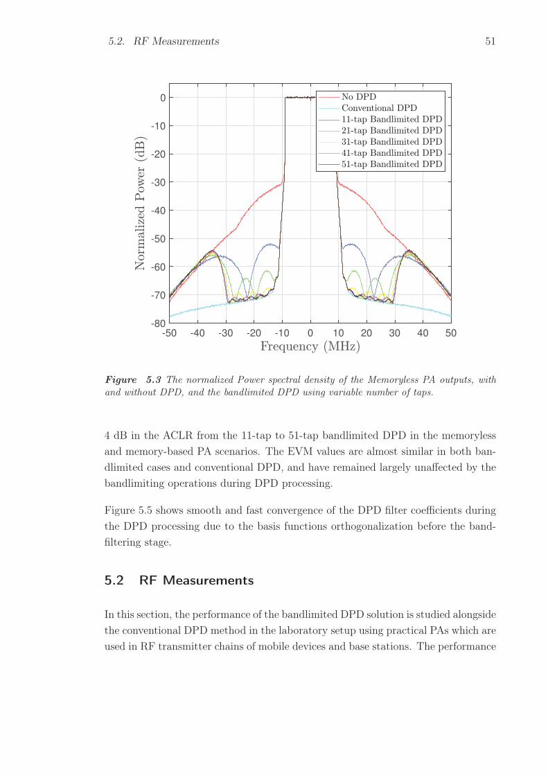
5.2. RF Measurements 51
-50 -40 -30 -20 -10 0 10 20 30 40 50-80
-70
-60
-50
-40
-30
-20
-10
0
Figure 5.3 The normalized Power spectral density of the Memoryless PA outputs, withand without DPD, and the bandlimited DPD using variable number of taps.
4 dB in the ACLR from the 11-tap to 51-tap bandlimited DPD in the memorylessand memory-based PA scenarios. The EVM values are almost similar in both ban-dlimited cases and conventional DPD, and have remained largely unaffected by thebandlimiting operations during DPD processing.
Figure 5.5 shows smooth and fast convergence of the DPD filter coefficients duringthe DPD processing due to the basis functions orthogonalization before the band-filtering stage.
5.2 RF Measurements
In this section, the performance of the bandlimited DPD solution is studied alongsidethe conventional DPD method in the laboratory setup using practical PAs which areused in RF transmitter chains of mobile devices and base stations. The performance

5.2. RF Measurements 52
-50 -40 -30 -20 -10 0 10 20 30 40 50
-60
-50
-40
-30
-20
-10
0
Figure 5.4 The normalized Power spectral density of the Memory-based PA outputs, withand without DPD, and the bandlimited DPD using variable number of taps.
of the bandlimited DPD solution in practical PA environment is further quantifiedusing the EVM and ACLR metrics used in the simulation environment to allow fora fair comparison between the two environments. Although the simulation resultsprove that the bandlimited DPD solution suppresses the PA nonlinearity in thepredefined band, it is necessary to confirm and additionally demonstrate using trueRF measurements that the bandlimited DPD solution can be used in the actualtransmitter environments.
In the subsequent subsections, the measurement setup and the hardware componentsare discussed in details. The performance of the bandlimited DPD solution is thenquantified, and finally we compare the results in the practical PA scenarios withthose achieved in the simulation environment.

5.2. RF Measurements 53
Table 5.1 Comparison of the linearization performance of the bandlimited DPD with theConventional DPD using the EVM and ACLR measures, for the memoryless PA model.
PAPR = 8.20 dB EVM [%] ACLR L/R(dBc)No DPD 3.6481 33.224/33.214With Conventional DPD 0.0275 54.809/54.46611-tap Bandlimited DPD 0.0579 51.103/50.9221-tap Bandlimited DPD 0.0635 54.306/53.98931-tap Bandlimited DPD 0.0735 54.717/54.38741-tap Bandlimited DPD 0.0999 54.768/54.42551-tap Bandlimited DPD 0.1076 54.776/54.441
Table 5.2 Comparison of the linearization performance of the bandlimited DPD with theConventional DPD using the EVM and ACLR measures, for the memory-based PA model.
PAPR = 8.18 dB EVM [%] ACLR L/R(dBc)No DPD 5.4084 33.733/33.788With Conventional DPD 0.3594 50.939/51.57711-tap Bandlimited DPD 0.3614 49.822/50.04821-tap Bandlimited DPD 0.3610 52.234/52.55131-tap Bandlimited DPD 0.3656 52.511/52.99241-tap Bandlimited DPD 0.3692 52.595/53.11551-tap Bandlimited DPD 0.3710 52.707/53.138
5.2.1 Hardware Description and Measurement Setup
The measurement setup used in the RF measurements is shown in Figure 5.6, and iscomposed of state-of-the-art vector signal transceiver (VST), low-cost power atten-uators, and a commercial LTE-A user equipment (UE) and base station (BS) PAs.Two scenarios are evaluated in the RF measurements. First, a UE scenario wherethe proposed DPD solution performance is evaluated using a LTE-A mobile devicePA in an uplink transmission environment. In the second scenario, the bandlimitedDPD solution is employed in a downlink BS environment using a commercial highpower amplifier (HPA).
The National Instruments (NI) PXIe-5840 VST is employed in our measurements.It combines a vector signal generator (VSG), a vector signal analyzer (VSA), anda high-speed serial data interface. The VST has a frequency range from 9 KHz to6.5 GHz and a 1 GHz instantaneous bandwidth which are highly desirable in thetesting and prototyping of wide bandwidth applications involving carrier aggregation

5.2. RF Measurements 54
0 0.5 1 1.5 2 2.5 30
10
20
30
40
50
60
Figure 5.5 Convergence of the the DPD filter coefficients of the 21-tap bandlimited DPDfor the memory-based PA model. It exemplifies fast and steady convergence of the DPDfilter coefficients in the bandlimited DPD system.
scenarios. The VST performs RF I/Q modulation and demodulation while a hostprocessor, embedded through a NI PXIe-8880 controller, runs the bandlimited DPDsolution.
An LTE-A input signal composed of one 20 MHz DL OFDM(A) component carrier(CC) with 16-QAM data modulation scheme is also employed in the RF measure-ment scenarios. Prior to the DPD processing, the transmit signal undergoes throughCFR by iterative clipping and filtering. In the conventional DPD method (imple-mented for reference), the DPD running bandwidth is set to 200 MHz, and theentire nonlinearity profile of the PA is linearized. In the bandlimited case, only theinband and OOB distortions in the immediate vicinity in the carrier are targeted;and consequently the DPD running bandwidth is restrained to 3-times less thanconventional bandwidth (i.e. 66.6 MHz) using the 21-tap LS FIR filter. The ban-

5.2. RF Measurements 55
VariableAttenuator(s)
Mobile PA
Vector SignalTransceiver
VST RF Out
VST RF In
Host processor based Processing Generate I/Q data samples for CC(s). Transfer blocks of size K samples
iteratively to VST for RF upconversionand I/Q modulation.
Extract received data blocks from VSTafter RF downconversion and I/Qdemodulation.
Estimate the bandlimited DPD parameters
Figure 5.6 Hardware setup used in the laboratory RF measurement. The setup is usedfor the UE measurement, while in the BS measurements the mobile PA is replaced by theBS PA and a driver PA.
dlimited output signal is then down-sampled by a factor of 3 to reduce the DPDsample rate. The above DPD processing parameters are used in both UE and BSmeasurement scenarios.
5.2.2 UE Measurement Results
The ACPM-5002-TR1 mobile device PA, which has a 29-dB gain and +31-dBm1-dB compression point, is used for the UE measurements. It is designed for mobiledevice transmitters for uplink propagation in LTE-A band 25 (1850-1915 MHz).The PA input signal is centred at 1880 MHz for optimum performance of the PA.
The block adaptive decorrelation-based parameter learning is used for the evaluationand quantification of the bandlimited DPD solution. The host processor generatesthe digital baseband input signal, which is then subdivided into 8 parameter learningblocks of size K = 50k samples each. The blocks are then transferred iteratively tothe VSG for RF upconversion and I/Q modulation to the PA transmit frequencyrange and at desired input power level. The VSG output signal is then relayed to thePA input port via the VST RF output port. The PA feedback observation signal iscoupled back to the VST RF input port through two attenuators, the 8493A coaxialfixed attenuator and the SMA fixed attenuator, whose resultant attenuation is 40dB.
The VSA then performs RF downconversion and I/Q demodulation to bring the
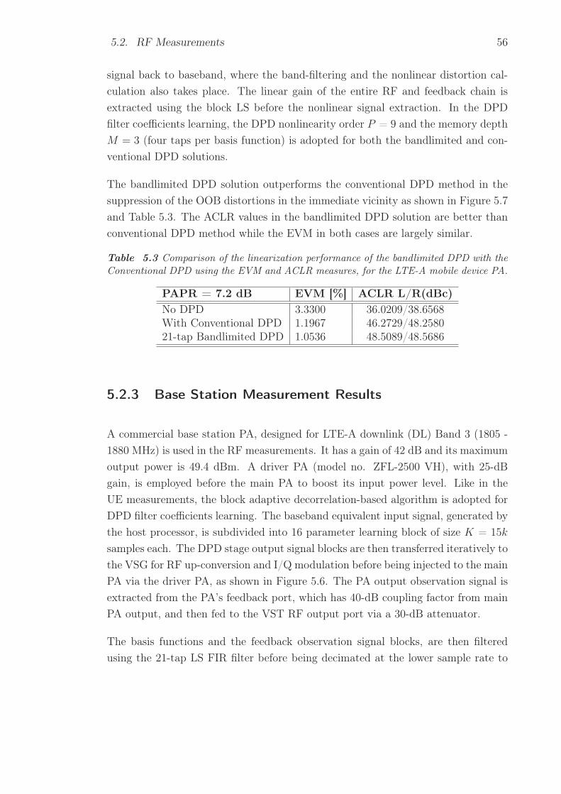
5.2. RF Measurements 56
signal back to baseband, where the band-filtering and the nonlinear distortion cal-culation also takes place. The linear gain of the entire RF and feedback chain isextracted using the block LS before the nonlinear signal extraction. In the DPDfilter coefficients learning, the DPD nonlinearity order P = 9 and the memory depthM = 3 (four taps per basis function) is adopted for both the bandlimited and con-ventional DPD solutions.
The bandlimited DPD solution outperforms the conventional DPD method in thesuppression of the OOB distortions in the immediate vicinity as shown in Figure 5.7and Table 5.3. The ACLR values in the bandlimited DPD solution are better thanconventional DPD method while the EVM in both cases are largely similar.
Table 5.3 Comparison of the linearization performance of the bandlimited DPD with theConventional DPD using the EVM and ACLR measures, for the LTE-A mobile device PA.
PAPR = 7.2 dB EVM [%] ACLR L/R(dBc)No DPD 3.3300 36.0209/38.6568With Conventional DPD 1.1967 46.2729/48.258021-tap Bandlimited DPD 1.0536 48.5089/48.5686
5.2.3 Base Station Measurement Results
A commercial base station PA, designed for LTE-A downlink (DL) Band 3 (1805 -1880 MHz) is used in the RF measurements. It has a gain of 42 dB and its maximumoutput power is 49.4 dBm. A driver PA (model no. ZFL-2500 VH), with 25-dBgain, is employed before the main PA to boost its input power level. Like in theUE measurements, the block adaptive decorrelation-based algorithm is adopted forDPD filter coefficients learning. The baseband equivalent input signal, generated bythe host processor, is subdivided into 16 parameter learning block of size K = 15ksamples each. The DPD stage output signal blocks are then transferred iteratively tothe VSG for RF up-conversion and I/Q modulation before being injected to the mainPA via the driver PA, as shown in Figure 5.6. The PA output observation signal isextracted from the PA’s feedback port, which has 40-dB coupling factor from mainPA output, and then fed to the VST RF output port via a 30-dB attenuator.
The basis functions and the feedback observation signal blocks, are then filteredusing the 21-tap LS FIR filter before being decimated at the lower sample rate to

5.2. RF Measurements 57
1820 1840 1860 1880 1900 1920 1940
-60
-50
-40
-30
-20
-10
0
Figure 5.7 The normalized PA output power spectral density of the conventional DPDcompared to the 21-tap bandlimited DPD for a UE LTE-A PA for a single 20 MHz compo-nent carrier operating at an output power of +21 dBm.
reduce the DPD running bandwidth and complexity. The DPD filter coefficientsare then computed using the block adaptive decorrelation-based principle and usedto filter the next block of parameters. Like in the UE measurements, the DPDnonlinearity order P = 9 and the memory depth M = 3 (four taps per basis function)are adopted for both the bandlimited and conventional DPD solutions.
Figure 5.8 and Table 5.4 shows the normalized PSDs of the bandlimited DPD solu-tion compared to the conventional DPD method and the corresponding EVM andACLR results, respectively. The results further confirm better performance of thebandlimited DPD in the ACLR measurement region, despite using fewer samples inthe DPD learning blocks to reduce computational complexity.
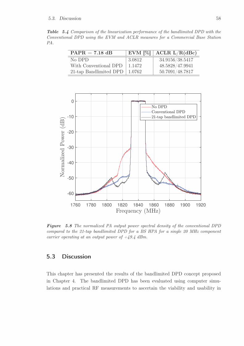
5.3. Discussion 58
Table 5.4 Comparison of the linearization performance of the bandlimited DPD with theConventional DPD using the EVM and ACLR measures for a Commercial Base StationPA.
PAPR = 7.18 dB EVM [%] ACLR L/R(dBc)No DPD 3.0812 34.9156/38.5417With Conventional DPD 1.1472 48.5828/47.994121-tap Bandlimited DPD 1.0762 50.7091/48.7817
1760 1780 1800 1820 1840 1860 1880 1900 1920
-60
-50
-40
-30
-20
-10
0
Figure 5.8 The normalized PA output power spectral density of the conventional DPDcompared to the 21-tap bandlimited DPD for a BS HPA for a single 20 MHz componentcarrier operating at an output power of +49.4 dBm.
5.3 Discussion
This chapter has presented the results of the bandlimited DPD concept proposedin Chapter 4. The bandlimited DPD has been evaluated using computer simu-lations and practical RF measurements to ascertain the viability and usability in

5.3. Discussion 59
the real transmitter chain environments. The proposed DPD solution performanceis compared to the conventional DPD method in two computer simulation scenar-ios using memoryless and memory-based PH PA models as well as commercial UEand BS PAs. The DPD running bandwidth is reduced by filtering the PA feed-back observation signal and basis functions using FIR filters thereby reducing theband linearized using DPD. To reduce computational complexity, the sample ratesof the bandlimited DPD solution are reduced by decimating the signals prior to thedecorrelation-based learning. In all the above scenarios, there is a reduction in theminimum required DPD sample rates. For instance, in the simulation studies, thesample rates are reduced from 180 MSPS to 100 MSPS, which consequently leadsto a significant reduction in the number of FLOPs per second (FLOPs) required forthe generation of basis functions and DPD coefficients filtering.
The memoryless PA model results show a consistent tread in the improvement ofACLR of the bandlimited DPD solution as the number of filter taps, which is ratherobvious. However, as the filter taps increase, there is no significant increase inthe ACLR and the value tends to approach the conventional DPD’s value. In thememory-based PA model and practical PAs RF measurements, the bandlimitedDPD solution outperforms the conventional DPD method when filter taps are equalor more than 21. This is attributed to the application of the DPD filter coefficientson a narrower frequency band thereby outperforming the conventional DPD methodin the suppression of the spectral regrowth in the ACLR measurement region. Inall the bandlimited DPD solution scenarios, the EVM values remain largely similarwith the corresponding conventional DPD values, implying a good performance inthe restoration of the inband waveform purity.
The results are consistent in the memory-based PA model and the commercial PAs,which is an interesting finding, in that the bandlimited DPD solution offers an extra 1- 2 dB spectral regrowth suppression. The bandlimited decorrelation-based learningmay become inevitable when extra distortion cancellation is required to suppress apersistent part of the spectral regrowth because of the sample rates reduction andimproved ACLR performance. Furthermore, the solution offers a computationally-efficient process which is attractive for the battery powered devices and small BSs.However, for the benefits of the bandlimited DPD solution to be fully leveraged,the extra computations introduced by the filter functions fn should be less than thereduction in computations obtained from using lower DPD sample rates. In thisway, the power consumption of the entire RF transmission chain is reduced while

5.3. Discussion 60
achieving better unwanted emission suppression.

61
6. CONCLUSION
In this thesis, a bandlimited DPD solution is studied for mitigation of nonlineardistortion in wideband spectrum access involving a single carrier or contiguous CA oftwo or more CCs. The reduced-complexity decorrelation-based principle formulatedin [14] for suppression of unwanted emissions is applied in the studied bandlimitedDPD concept. The performance of the bandlimited DPD solution is compared tothe conventional DPD method using the well-known ACLR and EVM metrics.
The studied bandlimited DPD solution involves the use of DPD for the suppressionof the inband distortion and spectrum regrowth in the immediate vicinity, whileunwanted emissions more far away in the spectrum from the main carrier(s) aresuppressed using transmit filters or ignored if they don’t violate the emission limits.The use of wide bandwidths of up to 100 MHz proposed in future LTE-A implemen-tations may make classical DPD methods infeasible due to the high speed require-ments for the DACs, transmitter, and receiver chains. Recent works in literaturehave concentrated in the development of the bandlimited DPD methods using theILA, which is more computationally-complex compared to the decorrelation basedprinciple.
The bandlimited DPD solution studied aims at reducing the DPD running band-width using FIR filters to limit the bandwidth expansion during basis functionsgeneration and to filter the bandwidth of the feedback observation signal from thePA output. The resultant signal blocks are then decimated to reduce the samplerates, before the DPD filter coefficients are computed using the decorrelation-basedlearning, as explained in Chapter 4. The DPD processing stage therefore becomescomputationally-efficient due to reduction in the number of computations performedon the parameters to obtain the DPD filter coefficients. Furthermore, the PH PAmodel used in the generation of the basis functions requires less running complex-ity than Volterra series and is shown to accurately model nonlinear distortions inpractical PAs [17].

6. Conclusion 62
To ascertain the viability of the bandlimited DPD solution, Matlab-based simula-tions using PH PA models extracted from practical PAs as well as true RF mea-surements using commercial PAs used in RF front-ends were performed. The firstscenario involved the use of a memoryless PH PA model in which the bandlimitedDPD solution is outperformed by the conventional DPD method in both the suppres-sion of the inband distortions and OOB emissions in all the cases. However, thereis an improvement in the ACLR performance as the number of filter taps increase.The other matlab-based simulation scenario involves the use of the memory-basedPH PA model, while the RF measurements utilize two commercial PAs used inUE and BS transmitter chains. In all the scenarios, the bandlimited DPD solutionperforms better than the conventional DPD method in the suppression of spectralregrowth within the ACLR measurement regions when an FIR filter with 21 or moretaps is used. The achieved inband waveform purity is largely similar for all the testruns. Overall, the ACLR values are approximately 1-2 dB higher than those of theconventional DPD method.
The bandlimited DPD solution explored offers better linearization performance un-der hardware and software constraints due to its low-complexity decorrelation-basedlearning principle. Furthermore, the solution alleviates the DPD bandwidth con-straints associated with wideband LTE-A implementations by offering designers flex-ibility to choose the bandwidth to be linearized. The practical applicability of thebandlimited DPD solution is therefore enhanced, as the linearization performanceis improved while reducing the complexity of the DPD.

63
BIBLIOGRAPHY
[1] LTE Evolved Universal Terrestrial Radio Access (E-UTRA): User Equipment(UE) Radio Transmission and Reception, document 3GPP TS 36.101 V13.3.0(Release 13), May 2016.
[2] J. Proakis and M. Salehi, Digital Communications. McGraw-Hill, 2008.[Online]. Available: https://books.google.fi/books?id=IllBngAACAAJ
[3] G. Fettweis, M. Lohning, D. Petrovic, M. Windisch, P. Zillmann, and W. Rave,“Dirty rf: a new paradigm,” in 2005 IEEE 16th International Symposium onPersonal, Indoor and Mobile Radio Communications, vol. 4, Sept 2005, pp.2347–2355 Vol. 4.
[4] A. M. Wyglinski, “Physical layer loading algorithms for indoor wireless multi-carrier systems,” Ph.D. dissertation, McGill University, 2004.
[5] S. Cripps, RF Power Amplifiers for Wireless Communications, ser. ArtechHouse microwave library.
[6] Unwanted Emissions in the Spurious Domain, document Rec. ITU-R SM.329-12, Int. Telecommun. Union Radio Commun. Sector, Sep. 2012.
[7] A. Kiayani, M. Abdelaziz, L. Anttila, V. Lehtinen, and M. Valkama, “Digitalmitigation of transmitter-induced receiver desensitization in carrier aggregationfdd transceivers,” IEEE Transactions on Microwave Theory and Techniques,vol. 63, no. 11, pp. 3608–3623, Nov 2015.
[8] M. Abdelaziz, L. Anttila, and M. Valkama, “Digital predistortion for miti-gating transmitter-induced receiver desensitization in carrier aggregation fddtransceivers,” in 2016 IEEE Global Conference on Signal and Information Pro-cessing (GlobalSIP), Dec 2016, pp. 694–698.
[9] A. Katz, "Linearization: reducing distortion in power amplifiers," in IEEEMicrowave Magazine, vol. 2, no. 4, pp. 37-49, Dec 2001.
[10] A. Mohammadi and F. M. Ghannouchi, RF Power Amplifier and LinearizationTechniques. Berlin, Heidelberg: Springer Berlin Heidelberg, 2012, pp. 77–128.
BIBLIOGRAPHY 64
[11] J. K. Cavers, “Amplifier linearization using a digital predistorter with fast adap-tation and low memory requirements,” IEEE Transactions on Vehicular Tech-nology, vol. 39, no. 4, pp. 374–382, Nov 1990.
[12] W.-J. Kim, S. P. Stapleton, J. H. Kim, and C. Edelman, “Digital predistortionlinearizes wireless power amplifiers,” IEEE Microwave Magazine, vol. 6, no. 3,pp. 54–61, Sept 2005.
[13] F. Luo, Digital Front-End in Wireless Communications and Broadcasting:Circuits and Signal Processing. Cambridge University Press, 2011. [Online].Available: https://books.google.fi/books?id=Tu_c9XmSD1UC
[14] M. Abdelaziz, L. Anttila, C. Tarver, K. Li, J. R. Cavallaro, and M. Valkama,“Low-complexity subband digital predistortion for spurious emission suppres-sion in noncontiguous spectrum access,” IEEE Transactions on Microwave The-ory and Techniques, vol. 64, no. 11, pp. 3501–3517, Nov 2016.
[15] Z. Fu, L. Anttila, M. Abdelaziz, M. Valkama, and A. M. Wyglinski, “Frequency-selective digital predistortion for unwanted emission reduction,” IEEE Trans-actions on Communications, vol. 63, no. 1, pp. 254–267, Jan 2015.
[16] M. Abdelaziz, A. Ghazi, L. Anttila, J. Boutellier, T. Lähteensuo, X. Lu, J. R.Cavallaro, S. S. Bhattacharyya, M. Juntti, and M. Valkama, “Mobile trans-mitter digital predistortion: Feasibility analysis, algorithms and design explo-ration,” in 2013 Asilomar Conference on Signals, Systems and Computers, Nov2013, pp. 2046–2053.
[17] A. S. Tehrani, H. Cao, S. Afsardoost, T. Eriksson, M. Isaksson, and C. Fager,“A comparative analysis of the complexity/accuracy tradeoff in power amplifierbehavioral models,” IEEE Transactions on Microwave Theory and Techniques,vol. 58, no. 6, pp. 1510–1520, June 2010.
[18] J. C. Pedro and S. A. Maas, “A comparative overview of microwave and wire-less power-amplifier behavioral modeling approaches,” IEEE Transactions onMicrowave Theory and Techniques, vol. 53, no. 4, pp. 1150–1163, April 2005.
[19] M. Isaksson, D. Wisell, and D. Ronnow, “A comparative analysis of behavioralmodels for rf power amplifiers,” IEEE Transactions on Microwave Theory andTechniques, vol. 54, no. 1, pp. 348–359, Jan 2006.

BIBLIOGRAPHY 65
[20] C. Yu, L. Guan, and A. Zhu, “Band-limited volterra series-based behavioralmodeling of rf power amplifiers,” in 2012 IEEE/MTT-S International Mi-crowave Symposium Digest, June 2012, pp. 1–3.
[21] C. Yu, L. Guan, E. Zhu, and A. Zhu, “Band-limited volterra series-based digi-tal predistortion for wideband rf power amplifiers,” IEEE Transactions on Mi-crowave Theory and Techniques, vol. 60, no. 12, pp. 4198–4208, Dec 2012.
[22] M. Abdelaziz, L. Anttila, A. Mohammadi, F. Ghannouchi, and M. Valkama,“Reduced-complexity power amplifier linearization for carrier aggregation mo-bile transceivers,” in 2014 IEEE International Conference on Acoustics, Speechand Signal Processing (ICASSP), May 2014, pp. 3908–3912.
[23] M. Abdelaziz, L. Anttila, A. Kiayani, and M. Valkama, “Decorrelation-basedconcurrent digital predistortion with a single feedback path,” IEEE Transac-tions on Microwave Theory and Techniques, vol. PP, no. 99, pp. 1–14, 2017.
[24] F. M. Ghannouchi and O. Hammi, “Behavioral modeling and predistortion,”IEEE Microwave Magazine, vol. 10, no. 7, pp. 52–64, Dec 2009.
[25] J. H. K. Vuolevi and T. Rahkonen, “Extraction of a nonlinear ac fet modelusing small-signal s-parameters,” IEEE Transactions on Microwave Theory andTechniques, vol. 50, no. 5, pp. 1311–1315, May 2002.
[26] P. Asbeck, “Linearisation of rf power amplifiers,” Ph.D. dissertation, TechnicalUniversity of Denmark, 2001.
[27] R. Raich and G. T. Zhou, “On the modeling of memory nonlinear effects ofpower amplifiers for communication applications,” in Proceedings of 2002 IEEE10th Digital Signal Processing Workshop, 2002 and the 2nd Signal ProcessingEducation Workshop., Oct 2002, pp. 7–10.
[28] R. Raich, “Nonlinear system identification and analysis with applications topower amplifier modeling and power amplifier predistortion,” Ph.D. disserta-tion, Georgia Institute of Technology, 2004.
[29] A. E. Nordsjo, “An algorithm for adaptive predistortion of certain time-varyingnonlinear high-power amplifiers,” in RADAR 2002, Oct 2002, pp. 469–473.
[30] J. Voros, “Modeling and identification of wiener systems with two-segment non-linearities,” IEEE Transactions on Control Systems Technology, vol. 11, no. 2,pp. 253–257, Mar 2003.

BIBLIOGRAPHY 66
[31] A. A. M. Saleh, “Frequency-independent and frequency-dependent nonlinearmodels of twt amplifiers,” IEEE Transactions on Communications, vol. 29,no. 11, pp. 1715–1720, November 1981.
[32] E. Costa, M. Midrio, and S. Pupolin, “Impact of amplifier nonlinearities on ofdmtransmission system performance,” IEEE Communications Letters, vol. 3, no. 2,pp. 37–39, February 1999.
[33] Y. Guo and J. R. Cavallaro, “A novel adaptive pre-distorter using ls estima-tion of sspa non-linearity in mobile ofdm systems,” in 2002 IEEE InternationalSymposium on Circuits and Systems. Proceedings (Cat. No.02CH37353), vol. 3,2002, pp. III–453–III–456 vol.3.
[34] A. Ghorbani and M. Sheikhan, “The effect of solid state power amplifiers (sspas)nonlinearities on mpsk and m-qam signal transmission,” in 1991 Sixth Inter-national Conference on Digital Processing of Signals in Communications, Sep1991, pp. 193–197.
[35] C. Rapp, “Effects of HPA-nonlinearity on a 4DPSK/OFDMsignal for a digitalsound broadcasting system, “in Proceedings of the Second European Conferenceon Satellite Communications, pp. 179- 184,Liege, Belgium, Oct. 22-24, 1991.
[36] G. P. White, A. G. Burr, and T. Javornik, “Modelling of nonlinear distortionin broadband fixed wireless access systems,” Electronics Letters, vol. 39, no. 8,pp. 686–687, April 2003.
[37] S. Boumaiza and F. M. Ghannouchi, “Thermal memory effects modeling andcompensation in rf power amplifiers and predistortion linearizers,” IEEE Trans-actions on Microwave Theory and Techniques, vol. 51, no. 12, pp. 2427–2433,Dec 2003.
[38] J.Mathews and G. Sicuranza, Polynomial Signal Processing. New York, USA:John Wiley Sons, 2000.
[39] M. Schetzen, The Volterra and Wiener Theories of Nonlinear Systems, reprinted. Melbourne, FL: Krieger, 1989.
[40] A. Zhu, J. C. Pedro, and T. J. Brazil, “Dynamic deviation reduction-basedvolterra behavioral modeling of rf power amplifiers,” IEEE Transactions onMicrowave Theory and Techniques, vol. 54, no. 12, pp. 4323–4332, Dec 2006.

BIBLIOGRAPHY 67
[41] J. Kim and K. Konstantinou, “Digital predistortion of wideband signals basedon power amplifier model with memory,” Electronics Letters, vol. 37, no. 23,pp. 1417–1418, Nov 2001.
[42] D. R. Morgan, Z. Ma, J. Kim, M. G. Zierdt, and J. Pastalan, “A generalizedmemory polynomial model for digital predistortion of rf power amplifiers,” IEEETransactions on Signal Processing, vol. 54, no. 10, pp. 3852–3860, Oct 2006.
[43] F. M. Ghannouchi, O. Hammi, and M. Helaoui, Behavioral Modelling and Pre-distortion of Wideband Wireless Transmitters, 1st ed. GB: John Wiley SonsInc, 2015.
[44] J. Armstrong, “Peak-to-average power reduction for ofdm by repeated clippingand frequency domain filtering,” Electronics Letters, vol. 38, no. 5, pp. 246–247,Feb 2002.
[45] Jiang, T. and Wu, Y. (2008) An overview: peak-to-average power ratio reduc-tion techniques for OFDM signals. IEEE Transactions on Broadcasting , 54 (2),257– 268.
[46] Han, S.H. and Lee, J.H. (2005) An overview of peak-to-average power ratioreduction techniques for multi-carrier transmission. IEEE Wireless Communi-cations , 12 (2), 56– 65.
[47] P. Kenington, High-linearity RF Amplifier Design, ser. Artech Housemicrowave library. Artech House, 2000. [Online]. Available: https://books.google.fi/books?id=qQhTAAAAMAAJ
[48] H. Kosugi, T. Matsumoto, T. Uwano, "A High-Efficiency Linear Power Ampli-fier Using an Envelope Feedback Method", Electronics and Communications inJapan, Part 2, Vol. 77, No. 3, 1994.
[49] P. E. Kenington, High-linearity RF Amplifier Design , Artech House, 2000.
[50] D. Cox, “Linear amplification with nonlinear components,” IEEE Transactionson Communications, vol. 22, no. 12, pp. 1942–1945, Dec 1974.
[51] B. Stengel and W. R. Eisenstadt, “Linc power amplifier combiner method ef-ficiency optimization,” IEEE Transactions on Vehicular Technology, vol. 49,no. 1, pp. 229–234, Jan 2000.

Bibliography 68
[52] A. Bateman, “The combined analogue locked loop universal modulator (cal-lum),” in [1992 Proceedings] Vehicular Technology Society 42nd VTS Confer-ence - Frontiers of Technology, May 1992, pp. 759–763 vol.2.
[53] J. Wood, Behavioral Modeling and Linearization of RF Power Amplifiers. Nor-wood: Artech House Inc, 2014.
[54] H. Paaso and A. Mammela, “Comparison of direct learning and indirect learningpredistortion architectures,” in 2008 IEEE International Symposium on Wire-less Communication Systems, Oct 2008, pp. 309–313.
[55] R. N. Braithwaite, “A comparison of indirect learning and closed loop estima-tors used in digital predistortion of power amplifiers,” in 2015 IEEE MTT-SInternational Microwave Symposium, May 2015, pp. 1–4.
[56] M. Abdelaziz, L. Anttila, and M. Valkama, “Reduced-complexity digital predis-tortion for massive mimo,” in 2017 IEEE International Conference on Acous-tics, Speech and Signal Processing (ICASSP), March 2017, pp. 6478–6482.
[57] H. Qian, S. Yao, H. Huang, and W. Feng, “A low-complexity digital predistor-tion algorithm for power amplifier linearization,” IEEE Transactions on Broad-casting, vol. 60, no. 4, pp. 670–678, Dec 2014.
[58] S. Haykin and S. Haykin, Adaptive Filter Theory. Pearson, 2014. [Online].Available: https://books.google.fi/books?id=J4GRKQEACAAJ
[59] 3GPP Evolved Universal Terrestrial Radio Access (E-UTRA); User Equip-ment (UE) radio transmission and reception, 3rd Generation Partner-ship Project (3GPP), Cedex, France. [Online]. Available: http://www.3gpp.org/ftp/Specs/html-info/36101.htm.
[60] J. Armstrong, “Peak-to-average power reduction for ofdm by repeated clippingand frequency domain filtering,” Electronics Letters, vol. 38, no. 5, pp. 246–247,Feb 2002.
[61] T. W. Parks and C. S. Burrus, Digital Filter Design, New York: John Wileyand Sons, Inc., June 1987, contains FORTRAN software listings.
[62] E. Dahlman, S. Parkvall, and J. Skold, 4G LTE/LTE-Advanced for MobileBroadband. Amsterdam, The Netherlands: Elsevier, 2011.
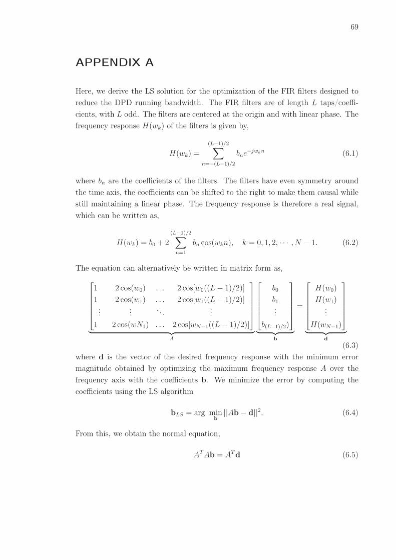
69
APPENDIX A
Here, we derive the LS solution for the optimization of the FIR filters designed toreduce the DPD running bandwidth. The FIR filters are of length L taps/coeffi-cients, with L odd. The filters are centered at the origin and with linear phase. Thefrequency response H(wk) of the filters is given by,
H(wk) =
(L−1)/2∑n=−(L−1)/2
bne−jwkn (6.1)
where bn are the coefficients of the filters. The filters have even symmetry aroundthe time axis, the coefficients can be shifted to the right to make them causal whilestill maintaining a linear phase. The frequency response is therefore a real signal,which can be written as,
H(wk) = b0 + 2
(L−1)/2∑n=1
bn cos(wkn), k = 0, 1, 2, · · · , N − 1. (6.2)
The equation can alternatively be written in matrix form as,⎡⎢⎢⎢⎢⎣1 2 cos(w0) . . . 2 cos[w0((L− 1)/2)]
1 2 cos(w1) . . . 2 cos[w1((L− 1)/2)]...
... . . . ...1 2 cos(wN1) . . . 2 cos[wN−1((L− 1)/2)]
⎤⎥⎥⎥⎥⎦
︸ ︷︷ ︸A
⎡⎢⎢⎢⎢⎣
b0
b1...
b(L−1)/2)
⎤⎥⎥⎥⎥⎦
︸ ︷︷ ︸b
=
⎡⎢⎢⎢⎢⎣
H(w0)
H(w1)...
H(wN−1)
⎤⎥⎥⎥⎥⎦
︸ ︷︷ ︸d
(6.3)where d is the vector of the desired frequency response with the minimum errormagnitude obtained by optimizing the maximum frequency response A over thefrequency axis with the coefficients b. We minimize the error by computing thecoefficients using the LS algorithm
bLS = arg minb
||Ab− d||2. (6.4)
From this, we obtain the normal equation,
ATAb = ATd (6.5)

APPENDIX A 70
and finally, the optimum value of the coefficients b is given by
b = [(ATA)−1AT ]d. (6.6)