arX

iv:a

stro

-ph/

0702

206v

2 2

6 M

ar 2

007

Mon. Not. R. Astron. Soc. 000, 1–16 (2002) Printed 25 January 2018 (MN LATEX style file v2.2)

N-body Models of Rotating Globular Clusters

A. Ernst1,2⋆, P. Glaschke1,2, J. Fiestas1, A. Just1 and R. Spurzem1†

1Astronomisches Rechen-Institut / Zentr. Astron. Univ. Heidelberg, Monchhofstr. 12-14, 69120 Heidelberg, Germany2Max-Planck-Institut fur Astronomie, Konigstuhl 17, 69117 Heidelberg, Germany

Accepted ... Received ...

ABSTRACTWe have studied the dynamical evolution of rotating globular clusters with directN -body models. Our initial models are rotating King models; we obtained resultsfor both equal-mass systems and systems composed out of two mass components.Previous investigations using a Fokker-Planck solver have revealed that rotation hasa noticeable influence on stellar systems like globular clusters, which evolve by two-body relaxation. In particular, it accelerates their dynamical evolution through thegravogyro instability. We have validated the occurence of the gravogyro instability withdirect N -body models. In the case of systems composed out of two mass components,mass segregation takes place, which competes with the rotation in the acceleration ofthe core collapse. The “accelerating” effect of rotation has not been detected in ourisolated two-mass N -body models. Last, but not least, we have looked at rotating N -body models in a tidal field within the tidal approximation. It turns out that rotationincreases the escape rate significantly. A difference between retrograde and prograderotating star clusters occurs with respect to the orbit of the star cluster around theGalaxy, which is due to the presence of a “third integral” and chaotic scattering,respectively.

Key words: N -body simulations – rotating star clusters.

1 INTRODUCTION

This paper is devoted to an intriguing problem in the dy-namics of globular clusters: How an overall rotation of aglobular cluster affects its dynamical evolution. There is awealth of observational data which indicates that typicalglobular clusters are rotating. The first method for the de-tection of rotation in globular clusters dates back in the firsthalf of 20th century. Observations showed that “flattening”(i.e. a deviation of spherical symmetry) is a common fea-ture of globular clusters. The first ellipticity measurementshave been done by H. Shapley in the 1920s, see Shapley(1930). Subsequent ellipticity measurments of Galactic andextragalactic globular clusters have been done, among oth-ers, by Geisler & Hodge (1980), Frenk & Fall (1982), Geyeret al. (1983), White & Shawl (1987), Staneva, Spassova &Golev (1996). The ellipticities of Galactic globular clustersare now given in the Harris catalogue,1 cf. Harris (1996).A second method for the detection of rotation of globularclusters relies on radial velocity measurements of individ-ual stars in globulars (Wilson & Coffeen 1954, Mayor et al.

⋆ email: aernst@ari.uni-heidelberg.de† email: spurzem@ari.uni-heidelberg.de1 http://physwww.physics.mcmaster.ca/ harris/mwgc.dat

1984, Meylan & Mayor 1986, Gebhardt et al. 1994, 1995,2000, Reijns et al. 2006 and references therein). The mea-sured radial velocities can be plotted against the positionangle. The amplitude of a sine curve which is fitted throughthe data points serves as a rough measure (i.e. a lower limit)for the degree of rotation of the star cluster. Proper motionsof individual stars have been measured as well and used forthe detection of rotation in globular clusters (e.g. Peterson& Cudworth 1994, van Leeuwen et al. 2000 or Anderson &King 2003. The authors of the latter two references concludefor ω Cen and 47 Tuc that their axes of rotation are con-siderably inclined to the plane of the sky). Table 7.2 in thereview by Meylan & Heggie (1997) gives already an overviewof the degrees of rotation of Galactic globular clusters. Forinstance, Gebhardt et al. (1995) estimated Vrot/σ1D ≃ 0.2for the evolved clusters M15 and 47 Tuc. However, globu-lar clusters in the Large and Small Magellanic Clouds areyounger and markedly more elliptical than typical Galacticglobulars (see the above references), which suggests highervalues of Vrot/σ1D.

From the theoretical side, the first published study of arotating system of N = 100 bodies is the work by Aarseth(1969) which aimed at the dynamical evolution of clustersof galaxies. He already detected a flattening caused by rota-tion. Subsequent attempts to study rotating globular clus-

c© 2002 RAS

2 A. Ernst, P. Glaschke, J. Fiestas, A. Just & R. Spurzem

ters with direct N-body models have been made by Wielen(1974) for systems with particle numbers N = 50− 250 andAkiyama & Sugimoto (1989) for N = 1000. Wielen con-cludes that “a slow overall rotation of a globular clusterdoes not significantly affect the dynamical evolution”, andAkiyama & Sugimoto do not yet clearly demonstrate numer-ically the existence of the gravogyro instability (see below)“because of statistical noise due to a small number of par-ticles”. More recent numerical studies of rotating globularclusters have been done using the Fokker-Planck [hereafter:FP] method, see the PhD thesis of Einsel (1996), Einsel &Spurzem (1999) [hereafter ES99], the follow-up papers byKim et al. (2002, 2004) and the PhD thesis of Kim (2003)[hereafter K02, K03, K04]. Under certain approximations,the evolution of a phase space distribution function whichdescribes the macroscopic state of a globular cluster, is fol-lowed by the numerical solution of the FP equation. The ad-vantage of such approximate models is their computationalspeed, i.e. one can do large parameter studies in a reason-able time. For the most recent FP models including rotation,which are compared directly to observations of M5, M15, 47Tuc and ω Cen, see Fiestas et al. (2006).2

The present study is again concerned with N-bodymodels of rotating globular clusters. Based on Newton’s lawof gravitation, N-body modelling is probably the most di-rect way to investigate the dynamics of stars in globularclusters. However, it is computationally expensive and time-consuming.3 On the other hand, direct N-body modellingparticularly allows to test the validity of assumptions usedin statistical modelling of globular clusters, like FP models.

This paper is organized as follows: Section 2 describesour initial models and the numerical method. In Section 3we will have a closer look at the effect of rotation on thecore collapse in isolated equal-mass models. It is well-knownthat the core collapse is caused by the gravothermal insta-bility: The negative heat capacity of the self-gravitating coreof the star cluster leads to an amplification of temperaturegradients if the halo of the star cluster is extensive enough.The core collapse is stopped by the formation of a few bina-ries in the core of the star cluster by three-body processes(Giersz & Heggie 1994b, 1996). These produce heat at a rateslightly higher than the rate of energy loss due to two-bodyrelaxation, thereby cooling the cluster core which has nega-tive heat capacity. If the star cluster rotates, we numericallydemonstrate in Section 3 that an additional instability oc-curs: The gravogyro instability, which accelerates the corecollapse in our equal-mass models. In Section 4, which isdedicated to tidally limited models, we additionally studythe escape of stars from rotating star clusters, i.e. mass loss4

2 A database of rotating star cluster models exists at the ARI:http://www.ari.uni-heidelberg.de/clusterdata/3 Therefore N-body codes for massively parallel computers have

been written. Moreover, special-purpose hardware systems likeGRAPE boards have been in use for N-body simulations sincethe early 1990s (see http://grape.astron.s.u-tokyo.ac.jp/grape/).A new development is a technology based on FPGAs (Field Pro-grammable Gate Arrays). However, such hardware is not used inthe present study.4 The term “mass loss” is not used in the usual sense (due tostellar evolution), but in the sense of a mass loss of the whole starcluster through escaping stars (i.e. due to dynamical interactions).

across the tidal boundary. In Section 5, which treats rotat-ing systems composed out of two mass components, we studythe interplay between rotation and mass segregation.

2 INITIAL MODELS / NUMERICAL METHOD

We employ generalized King models with rotation. The dis-tribution function is given by

f(E, Jz) = C ·»

exp

„

−E −Φt

σ2

K

«

− 1

–

· exp„

−Ω0Jz

σ2

K

«

, (1)

which depends on the integrals of motion E (energy) and Jz

(z-component of angular momentum), where Φt is the po-tential at the outer boundary of the model (i.e. at the radiuswhere the density approaches zero), σK is the King velocitydispersion (which is not the central velocity dispersion) andΩ0 is close to the angular speed in the cluster center (whichhas nearly solid body rotation). In the distribution function(1), the first two factors on the right-hand side representjust a usual King model. The last factor, which depends onJz, introduces rotation into the model, i.e. a difference be-tween positive and negative Jz. It also allows for anisotropy,i.e. we have σr = σz 6= σφ for the velocity dispersions inradial, vertical and tangential directions, respectively. Notethat models where f ∝ exp(−γJz) have been first used byPrendergast & Tomer (1970) and Wilson (1975) to modelelliptical galaxies. However, this term in combination with aKing model has been first used in Goodman (1983, unpub-lished), then by Lagoute & Longaretti (1996), Longaretti &Lagoute (1996), Einsel (1996), ES99, K02, K03 and K04,Fiestas (2006) and Fiestas et al. (2006).

The rotating King model based on the distribution func-tion (1) possesses rotational symmetry and differential ro-tation. It has two dimensionless free parameters: The Kingparameter W0 = −(Φ0−Φt)/σ

2

K, where Φ0 is the central po-tential, and the rotation parameter ω0 =

p

9/(4πGρc) · Ω0,where G is the gravitational constant and ρc is the centraldensity. It reduces to a King model in the limit ω0 = 0.ES99 give the ratio λ = Trot/Tkin of rotational to kineticenergy in percent in their Table 1 for rotating King modelswith W0 = 6. The ratio of the root mean squared rota-tional velocity to the velocity dispersion is then given byVrot/σ1D =

p

3λ/(1− λ), which may be compared with ob-servations. Furthermore, it may be of interest to note thatbetween 0.7 < ω0 < 0.8 there is a transition where the initialaxisymmetric isolated rotating King models become unsta-ble to the formation of a bar (P. Berczik, priv. comm.).

Our models composed out of two mass componentsare initially uniformly mixed and characterized by two ad-ditional dimensionless parameters, the stellar mass ratioµ = m2/m1, where m1 and m2 are the individual massesof the light and heavy stars, respectively, and the mass frac-tion of heavy stars q = M2/M , where M2 is the total massof the heavy component and M is the total mass of the starcluster.

In direct N-body models, the main constraint for a rea-sonable computing time is the number of particles N . In oursimulations, we use N = 5000 for all models with µ 6 10(including all equal-mass models) and N = 32000 for mod-els with µ = 25 and µ = 50. A typical simulation for one of

c© 2002 RAS, MNRAS 000, 1–16

N-body Models of Rotating Globular Clusters 3

our equal-mass models took about three days on a 3 GHzPentium PC, until the core collapse time was reached.

The codes used are nbody6++ (e.g. Spurzem 1999)and nbody6 (see Aarseth 1999, 2003 for an overview). Theformer code is a variant of the latter modified in order torun on massively parallel computers. Both codes share, asidefrom parallelization, the same fundamental features andyield comparable results. A fourth-order Hermite scheme,applied first by Makino & Aarseth (1992), is used for thedirect integration of the Newtonian equations of motion ofthe N-body system. The codes use adaptive and individualtime steps, which are organized in hierarchical block timesteps, the Ahmad-Cohen neighbor scheme (Ahmad & Cohen1973), Kustaanheimo-Stiefel regularization of close encoun-ters (Kustaanheimo & Stiefel 1965) and Chain regularization(Mikkola & Aarseth 1990, 1993, 1996,1998).

All models done with nbody6++ have been calcu-lated on single-processor machines at the ARI, except thetwo-mass models TM9-TM12 (see section 5). Some models(from series EM2, see Section 3) have been calculated usingAarseth’s original code nbody6. For some models, we usedaveraging over several runs with the same particle numberN but different initial values for positions and velocities.This was done in order to obtain a better statistical quality,cf. Section 2.2 of Giersz & Heggie (1994a) for a discussionof this approach. Averaging increases the computing timefor gravitational forces of a system of N bodies on a linearscale, whereas increasing the particle number N increasesthe computing time for gravitational forces ∝ N2 in thelimit of high N . Since we consider in the present work pro-cesses acting on the relaxation time scale, an extra powerof N contributes to the scaling of the total computing timeof a model. In our averaged models, the physical quantitiesshown in the plots are determined as the arithmetic mean ofthose values of the considered quantity, which resulted fromthe individual runs.

The quantities on the vertical axis of our figures areshown in dimensionless N-body units, i.e. G = M = −4E =1, where G is the gravitational constant, M is the totalmass of the system and E the total energy, see Heggie &Mathieu (1986). The resulting length unit is the virial ra-dius rV = GM2/(−4E), which is of the order of the half-mass radius of a globular cluster, see, for instance, Table1 in Gurkan et al. (2004). The resulting time unit is thengiven by tV = (GM/r3V )−1/2. The time on the horizontalaxis of most figures is shown in units of the initial half-massrelaxation time, i.e. the trh means trh(0). For the half-massrelaxation time, we adopted the expression

trh =8π

3

h

p

2|E|/M rVi3

N

15.4G2 M2 ln(γN). (2)

with γ = 0.11. The above definition is based on Equation(5) of the paper by Spitzer & Hart (1971) with

n =3N

8πr3V, vm =

r

2|E|M

, m =M

N(3)

for the mean value of the particle density inside rV , the rootmean squared stellar velocity (i.e. the 3D velocity disper-

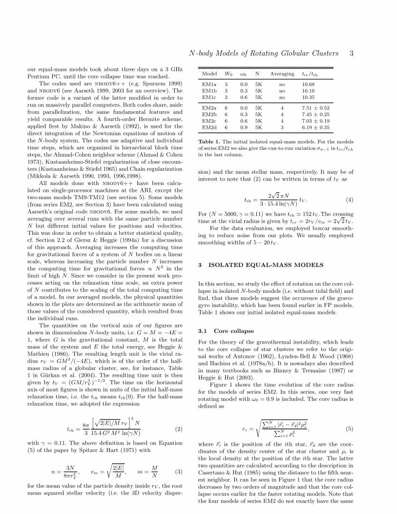
Model W0 ω0 N Averaging tcc/trh

EM1a 3 0.0 5K no 10.68EM1b 3 0.3 5K no 10.10EM1c 3 0.6 5K no 10.35

EM2a 6 0.0 5K 4 7.51 ± 0.52EM2b 6 0.3 5K 4 7.45 ± 0.25

EM2c 6 0.6 5K 4 7.03 ± 0.19EM2d 6 0.9 5K 3 6.19 ± 0.35

Table 1. The initial isolated equal-mass models. For the modelsof series EM2 we also give the run-to-run variation σn−1 in tcc/trhin the last column.

sion) and the mean stellar mass, respectively. It may be ofinterest to note that (2) can be written in terms of tV as

trh =2√2πN

3 · 15.4 ln(γN)tV . (4)

For (N = 5000, γ = 0.11) we have trh ≃ 152 tV .The crossingtime at the virial radius is given by tcr = 2rV /vm = 2

√2 tV .

For the data evaluation, we employed boxcar smooth-ing to reduce noise from our plots. We usually employedsmoothing widths of 5− 20 tV .

3 ISOLATED EQUAL-MASS MODELS

In this section, we study the effect of rotation on the core col-lapse in isolated N-body models (i.e. without tidal field) andfind, that these models suggest the occurence of the gravo-gyro instability, which has been found earlier in FP models.Table 1 shows our initial isolated equal-mass models.

3.1 Core collapse

For the theory of the gravothermal instability, which leadsto the core collapse of star clusters we refer to the origi-nal works of Antonov (1962), Lynden-Bell & Wood (1968)and Hachisu et al. (1978a/b). It is nowadays also describedin many textbooks such as Binney & Tremaine (1987) orHeggie & Hut (2003).

Figure 1 shows the time evolution of the core radiusfor the models of series EM2. In this series, one very fastrotating model with ω0 = 0.9 is included. The core radius isdefined as

rc =

s

PNi=1

|~ri − ~rd|2ρ2iPN

i=1ρ2i

, (5)

where ~ri is the position of the ith star, ~rd are the coor-dinates of the density center of the star cluster and ρi isthe local density at the position of the ith star. The lattertwo quantities are calculated according to the description inCasertano & Hut (1985) using the distance to the fifth near-est neighbor. It can be seen in Figure 1 that the core radiusdecreases by two orders of magnitude and that the core col-lapse occurs earlier for the faster rotating models. Note thatthe four models of series EM2 do not exactly have the same

c© 2002 RAS, MNRAS 000, 1–16

4 A. Ernst, P. Glaschke, J. Fiestas, A. Just & R. Spurzem

Figure 1. Time evolution of the core radius for the isolated mod-els EM2a-d.

Gravothermal instability Gravogyro instability

∂rσ2 6= 0 ∂rω 6= 0Negative specific heat Negative specific moment of

capacity inertiaEnergy transport Angular momentum transportHeat conduction Viscosity

Table 2. A comparison between gravothermal and gravogyro in-

stability.

initial core radius in the beginning, i.e. the core radii differby factors up to approximately two. This indicates that themodels are indeed not in all respects exactly comparable,cf. Figures 14/15 of K02. They have slightly different den-sity distributions corresponding to their degree of flattening.However, since the core shrinks by two orders of magnitudeduring the core collapse, a factor of two in the difference ofthe initial core radii seems to be negligible.

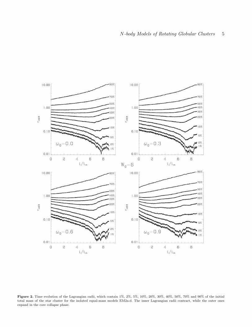
Figure 2 shows the time evolution of the Lagrangianradii for the models of series EM2. The inner Lagrangianradii shrink and the outer ones expand.

The last column of Table 1 contains the core collapsetimes for the isolated equal-mass models. The core collapsetime is defined as the time when the core radius rc reachedits first sharp minimum. For the averaged runs the giventime is the arithmetic mean of the core collapse times whichwe determined for each single run. We also give the standarddeviations σn−1 as a measure of the run-to-run variation ofthe core collapse times.

3.2 Gravogyro instability revisited - I

There is obviously a need to explain the accelerated corecollapse of the rotating models in Section 3.1. A theoreti-cal model, which explains such an effect, has been proposedas early as in the 1970s by Inagaki & Hachisu (1978) andHachisu (1979, 1982). They called it the gravogyro insta-bility. This instability is expected in self-gravitating androtating systems and has been derived for self-gravitatingcylinders of infinite length in z-direction: If we equate the

Figure 3. Time evolution of the z-component of the specific an-gular momentum of the particles within the Lagrangian radii forthe fast rotating isolated model EM2c. The isolated points areartefacts and stem (like the interruptions in the 1% curve) fromthe sign change of jz .

centrifugal force to the gravity in the equatorial plane (z =0, R2 = x2 + y2) and neglect the pressure gradient, we have

2GMR

R≃ j2z

R3, (6)

where MR is the mass per unit length in z-direction con-tained within the radius R in cylindrical coordinates and jzis the z-component of specific angular momentum. We read-ily obtain δjz/jz ≃ δR/R. Using the equation jz = R2ω inaddition, we obtain δjz ≃ ωRδR and δjz = 2ωRδR+R2δω.The combination of these relations yields the following lin-ear differential relation between specific angular momentumjz and angular speed ω:

δjz ≃ −R2δω. (7)

A negative specific moment of inertia occurs in this relation,cf. Inagaki & Hachisu (1978).

If we let an initial model evolve, which exhibits a radialgradient of the angular speed and has reasonable rotationcurve, angular momentum is transported outwards on therelaxation time scale by the stellar dynamical analog of vis-cosity. The core of the star cluster contracts because of adeficit in the centrifugal force. The angular speed in thecore increases according to relation (7). A runaway depar-ture from the initial state takes place. This cycle is whatthey denoted as the gravogyro instability. For a comparisonbetween gravothermal and gravogyro instabilities see Table2.

One may wonder: Does the gravogyro catastrophe re-ally occur in isolated N-body models? Figure 3 shows thetime evolution of the z-component of specific angular mo-mentum within the Lagrangian radii for the fast rotatingisolated model EM2c. The z-component of specific angularmomentum of each star is calculated according to

c© 2002 RAS, MNRAS 000, 1–16

N-body Models of Rotating Globular Clusters 5

Figure 2. Time evolution of the Lagrangian radii, which contain 1%, 2%, 5%, 10%, 20%, 30%, 40%, 50%, 70% and 90% of the initialtotal mass of the star cluster for the isolated equal-mass models EM2a-d. The inner Lagrangian radii contract, while the outer onesexpand in the core collapse phase.

c© 2002 RAS, MNRAS 000, 1–16

6 A. Ernst, P. Glaschke, J. Fiestas, A. Just & R. Spurzem

Figure 4. Time evolution of the average angular speed of the particles within the Lagrangian radii for the fast rotating isolated modelEM2c with W0 = 6, ω0 = 0.6. The interruptions and isolated points are artefacts stemming from the sign change of ω.

jz = [(~r⋆ − ~rd)× ~v⋆ ]z, (8)

where ~r⋆ = (x⋆, y⋆, z⋆) is the position of a particle, ~v⋆ =(v⋆x, v⋆y , v⋆z) is its velocity and ~rd = (xd, yd, zd) is the den-sity center of the star cluster. It is then summed over allparticles within a given Lagrangian radius and divided bythe number of particles inside that radius. One notes thatangular momentum does indeed diffuse from the inner partsof the cluster to the outer parts, as time proceeds.Now we study the evolution of the angular speed ω. Thegravogyro instability implies that jz goes down while ω in-creases. Figure 4 shows the time evolution of the averageangular speed of the particles within the Lagrangian radii.The angular speed of one particle is calculated according to

ω =jzR2

⋆=

[(~r⋆ − ~rd)× ~v⋆ ]zR2

⋆, (9)

with the same notations as in equation (8), but R⋆ =p

(x⋆ − xd)2 + (y⋆ − yd)2 is the radius with respect to thedensity center in cylindrical coordinates. It is then summedover all particles inside a given Lagrangian radius and di-vided by the number of particles within that radius. One canobserve an increasing average angular speed inside those La-grangian radii, which show a decrease in the z-component ofangular momentum. Thus, it is shown that gravogyro effectsappear in our isolated models.

4 TIDALLY LIMITED EQUAL-MASS MODELS

As a step towards more realistic models of globular clusters,we investigate in this section the effects of the tidal field ofthe Galaxy on the dynamical evolution of rotating globularclusters. The implementation of the tidal field of the MilkyWay Galaxy within the tidal approximation used in nbody6

and nbody6++ is in detail described in Appendix A. Dif-ferent escape criteria are discussed in Appendix B. In our

Model W0 ω0 N Averaging tcc/trh

EM3a 6 0.0 5K 4 7.11 ± 0.37EM3b 6 0.3 5K 4 6.37 ± 0.36EM3c 6 0.6 5K 4 5.42 ± 0.33EM3d 6 0.9 5K 4 3.97 ± 0.40

EM4b 6 -0.3 5K 4 6.50 ± 0.33EM4c 6 -0.6 5K 4 5.62 ± 0.07EM4d 6 -0.9 5K 4 4.88 ± 0.28

Table 3. The initial tidally limited equal-mass models. The rotat-ing models of series EM3 are prograde rotating while the modelsof series EM4 are retrograde rotating with respect to the orbit ofthe star cluster around the Galaxy. We also give the run-to-runvariation σn−1 in tcc/trh in the last column.

models, the star cluster initially completely fills its Rochelobe in the tidal field of the Galaxy. In other words, thedensity of the initial rotating King model approaches zeroat the physical tidal cutoff radius. The tidal radius is definedas the distance of the star cluster center to the Lagrangianpoints L1/L2.

Table 3 shows the initial tidally limited equal-massmodels. The model of series EM3 are prograde rotating, i.e.the stars move around the z-axis of the cluster-centered co-ordinate system in the same sense as the star cluster movesaround the Galaxy. The models of series EM5 are retrograderotating, which we denoted by a negative sign of the rota-tion parameter ω0 for clarity. The only difference betweenthe rotating initial models of series EM3 and EM4 is thatwe reversed the sign of all initial velocity vectors.

4.1 Core collapse

Figure 6 shows the time evolution of the core radius for theprograde rotating tidally limited models EM3a-d. A com-parison of Figures 1 and 6 and the core collapse times inTables 1 and 3 shows, that the tidal field further accelerates

c© 2002 RAS, MNRAS 000, 1–16

N-body Models of Rotating Globular Clusters 7

Figure 5. Time evolution of the total mass of the star clusters for the prograde rotating tidally limited models EM3a-d (lower solidlines), the retrograde rotating tidally limited models EM4b-c (upper solid lines), FP models with energy cutoff (dotted), two N-bodymodels with N = 5000 and energy cutoff (dashed) and one non-rotating N-body model with N = 16000 and energy cutoff (dot-dashed).The core collapse times of our N-body models are marked with a cross.

the core collapse by a significant amount. The reason for thisbehaviour is that rapid mass loss across the tidal boundaryprovides an additional mechanism for the transport and re-moval of energy and angular momentum, thus enhancing theeffects of the gravothermal and gravogyro instabilities. Aninspection of Table 3 reveals that there is a difference be-tween the core collapse times between the models of seriesEM3 and EM4, i.e. the prograde rotating models of seriesEM3 collapse faster than the retrograde rotating model ofseries EM4. By considering the run-to-run variation σn−1 inthe last column of table 3, we see that the statistical sig-nificance of this effect is strongest for the two models withω0 = 0.9 as compared with the case of the slower rotatingmodels.. Therefore this effect might be related to the forma-tion of a bar in the fastest rotating models. On the otherhand, the difference of the core collapse times between theprograde and retrograde rotating models may also be relatedto the difference in the rates of mass loss (see next Section):The loss of energy and angular momentum through escapingstars is more rapid for the prograde rotating models and thus

the effects of the gravothermal and gravogyro instabilities,which accelerate the core collapse, are stronger.

4.2 Mass loss

Figure 5 shows the time evolution of the total mass of theglobular clusters, where the initial mass is normalized toone, for several models, including simulations with the 2DFP code fopax (with energy cutoff, cf. Fiestas 2006), onerotating and one non-rotating N-body model by E. Kim(with energy cutoff, without the tidal approximation, seeK03) and one non-rotating N-body model by D. C. Heggie(with energy cutoff, without the tidal approximation). Thesolid lines are our nbody6++ results (with radius cutoffand the tidal approximation). The different “cutoffs” areexplained in Appendix B. The initial models are the samerotating (or non-rotating) King models. Note that for therotating models, there are two solid lines for each color. Thelower of these lines corresponds to a prograde rotating model(i.e., from series EM3). The upper of these lines correspondsto a retrograde rotating model (i.e., from series EM4). The

c© 2002 RAS, MNRAS 000, 1–16

8 A. Ernst, P. Glaschke, J. Fiestas, A. Just & R. Spurzem

Figure 6. Time evolution of the core radius for the prograderotating tidally limited models EM3a-d

escape rate for retrograde rotating models is considerablylower, since many stars in retrograde orbits are subject toa “third integral” of motion, which restricts their accessiblephase space and hinders them from escaping, see Fukushige& Heggie (2000) and Appendix B.

Figure 5 also shows, that the faster rotating models suf-fer stronger mass loss than the slowly or non-rotating mod-els, a fact which has already been shown in the FP modelsof ES99.

The differences between the models of the same rota-tion parameter are due to different implementations of thetidal field in the various codes (cf. Appendix B) or due tothe different modelling techniques in general. For instance,the difference between the N-body and FP models is thetidal approximation used in nbody6 and nbody6++, i.e.the modified equations of motion with a linear approxima-tion of the tidal forces (see Appendix A), a feature, whichcannot be implemented in an FP code, which relies onlyonly on a tidal cutoff. The geometry of the almond-shapedtidal boundary within the tidal approximation (see FigureB1) differs from the geometry of our star cluster models,which are axisymmetric. This may cause another differencebetween N-body and FP models. In addition, the differencebetween prograde and retrograde rotating models cannot beseen in FP models. Note that Kim et al. (2006) use for theircomparison N-body models with an artificially implementedtidal cutoff and no modification of the equations of motion.

Last but not least, a further inspection of Figure 5 re-veals, that core collapse causes an increase in the escape rate,i.e. short before the core collapse time the curves steepenslightly. The moment of core collapse is marked with a crosson each curve corresponding to one of our N-body mod-els. However, our main aim was to show the difference ofprograde and retrograde rotating models and the fact, thatrotation significantly increases the rate of mass loss.

4.3 Gravogyro instability revisited - II

In this subsection, we briefly look at the gravogyro insta-bility in the tidally limited N-body models. The mass lossthrough the tidal boundary provides, as noted before, anadditional mechanism for the transport and removal of an-

Figure 7. Time evolution of the Lagrangian radii for a single runof the fast rotating tidally limited model EM3c. For explanationssee the text.

Figure 8. Time evolution of the z-component of the specific an-gular momentum of the particles within the Lagrangian radii fora single run of the fast rotating tidally limited model EM3c. Forexplanations see the text.

gular momentum (besides viscosity effects). Figure 7 showsthe time evolution of the Lagrangian radii for one run ofthe tidally limited model EM3c. The Lagrangian radii aredefined with respect to the initial particle number. There-fore the particle number within the Lagrangian radii remainsconstant while the system evolves, whereas after some time,the outer Lagrangian shells are completely lost due to es-caping stars, i.e. the curves for the outer Lagrangian radiibend upwards until they reach twice the tidal radius, whichis the cutoff radius in the adopted escape criterion. Figure 8shows the time evolution of the z-component of specific an-gular momentum within the Lagrangian radii for the samesingle run of the tidally limited model EM3c. The curves forjz decrease due to escaping stars carrying away angular mo-mentum. The curves stop at the point at which the adjacentouter Lagrangian shell is lost, such that we always have aconstant particle number within the Lagrangian radii. Fig-ure 9 shows the time evolution of the average angular speed

c© 2002 RAS, MNRAS 000, 1–16

N-body Models of Rotating Globular Clusters 9

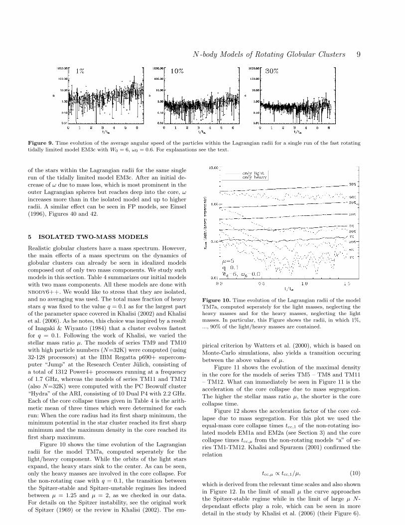
Figure 9. Time evolution of the average angular speed of the particles within the Lagrangian radii for a single run of the fast rotatingtidally limited model EM3c with W0 = 6, ω0 = 0.6. For explanations see the text.

of the stars within the Lagrangian radii for the same singlerun of the tidally limited model EM3c. After an initial de-crease of ω due to mass loss, which is most prominent in theouter Lagrangian spheres but reaches deep into the core, ωincreases more than in the isolated model and up to higherradii. A similar effect can be seen in FP models, see Einsel(1996), Figures 40 and 42.

5 ISOLATED TWO-MASS MODELS

Realistic globular clusters have a mass spectrum. However,the main effects of a mass spectrum on the dynamics ofglobular clusters can already be seen in idealized modelscomposed out of only two mass components. We study suchmodels in this section. Table 4 summarizes our initial modelswith two mass components. All these models are done withnbody6++. We would like to stress that they are isolated,and no averaging was used. The total mass fraction of heavystars q was fixed to the value q = 0.1 as for the largest partof the parameter space covered in Khalisi (2002) and Khalisiet al. (2006). As he notes, this choice was inspired by a resultof Inagaki & Wiyanto (1984) that a cluster evolves fastestfor q = 0.1. Following the work of Khalisi, we varied thestellar mass ratio µ. The models of series TM9 and TM10with high particle numbers (N=32K) were computed (using32-128 processors) at the IBM Regatta p690+ supercom-puter “Jump” at the Research Center Julich, consisting ofa total of 1312 Power4+ processors running at a frequencyof 1.7 GHz, whereas the models of series TM11 and TM12(also N=32K) were computed with the PC Beowulf cluster“Hydra” of the ARI, consisting of 10 Dual P4 with 2.2 GHz.Each of the core collapse times given in Table 4 is the arith-metic mean of three times which were determined for eachrun: When the core radius had its first sharp minimum, theminimum potential in the star cluster reached its first sharpminimum and the maximum density in the core reached itsfirst sharp maximum.

Figure 10 shows the time evolution of the Lagrangianradii for the model TM7a, computed seperately for thelight/heavy component. While the orbits of the light starsexpand, the heavy stars sink to the center. As can be seen,only the heavy masses are involved in the core collapse. Forthe non-rotating case with q = 0.1, the transition betweenthe Spitzer-stable and Spitzer-unstable regimes lies indeedbetween µ = 1.25 and µ = 2, as we checked in our data.For details on the Spitzer instability, see the original workof Spitzer (1969) or the review in Khalisi (2002). The em-

Figure 10. Time evolution of the Lagrangian radii of the modelTM7a, computed seperately for the light masses, neglecting theheavy masses and for the heavy masses, neglecting the lightmasses. In particular, this Figure shows the radii, in which 1%,..., 90% of the light/heavy masses are contained.

pirical criterion by Watters et al. (2000), which is based onMonte-Carlo simulations, also yields a transition occuringbetween the above values of µ.

Figure 11 shows the evolution of the maximal densityin the core for the models of series TM5 – TM8 and TM11– TM12. What can immediately be seen in Figure 11 is theacceleration of the core collapse due to mass segregation.The higher the stellar mass ratio µ, the shorter is the corecollapse time.

Figure 12 shows the acceleration factor of the core col-lapse due to mass segregation. For this plot we used theequal-mass core collapse times tcc,1 of the non-rotating iso-lated models EM1a and EM2a (see Section 3) and the corecollapse times tcc,µ from the non-rotating models “a” of se-ries TM1-TM12. Khalisi and Spurzem (2001) confirmed therelation

tcc,µ ∝ tcc,1/µ, (10)

which is derived from the relevant time scales and also shownin Figure 12. In the limit of small µ the curve approachesthe Spitzer-stable regime while in the limit of large µ N-dependant effects play a role, which can be seen in moredetail in the study by Khalisi et al. (2006) (their Figure 6).

c© 2002 RAS, MNRAS 000, 1–16

10 A. Ernst, P. Glaschke, J. Fiestas, A. Just & R. Spurzem

Figure 11. Time evolution of the maximal density in the core for the models of series TM5 – TM8 and TM11 – TM12

c© 2002 RAS, MNRAS 000, 1–16

N-body Models of Rotating Globular Clusters 11

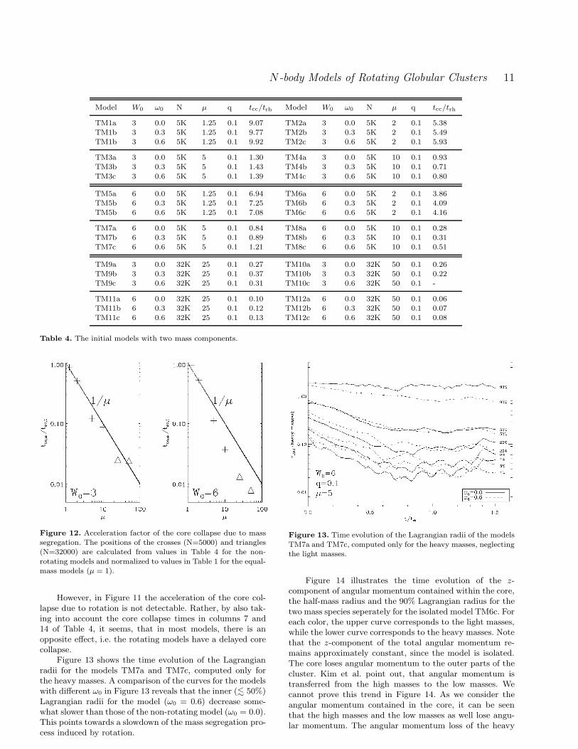
Model W0 ω0 N µ q tcc/trh Model W0 ω0 N µ q tcc/trh

TM1a 3 0.0 5K 1.25 0.1 9.07 TM2a 3 0.0 5K 2 0.1 5.38TM1b 3 0.3 5K 1.25 0.1 9.77 TM2b 3 0.3 5K 2 0.1 5.49TM1b 3 0.6 5K 1.25 0.1 9.92 TM2c 3 0.6 5K 2 0.1 5.93

TM3a 3 0.0 5K 5 0.1 1.30 TM4a 3 0.0 5K 10 0.1 0.93TM3b 3 0.3 5K 5 0.1 1.43 TM4b 3 0.3 5K 10 0.1 0.71

TM3c 3 0.6 5K 5 0.1 1.39 TM4c 3 0.6 5K 10 0.1 0.80

TM5a 6 0.0 5K 1.25 0.1 6.94 TM6a 6 0.0 5K 2 0.1 3.86TM5b 6 0.3 5K 1.25 0.1 7.25 TM6b 6 0.3 5K 2 0.1 4.09TM5b 6 0.6 5K 1.25 0.1 7.08 TM6c 6 0.6 5K 2 0.1 4.16

TM7a 6 0.0 5K 5 0.1 0.84 TM8a 6 0.0 5K 10 0.1 0.28TM7b 6 0.3 5K 5 0.1 0.89 TM8b 6 0.3 5K 10 0.1 0.31TM7c 6 0.6 5K 5 0.1 1.21 TM8c 6 0.6 5K 10 0.1 0.51

TM9a 3 0.0 32K 25 0.1 0.27 TM10a 3 0.0 32K 50 0.1 0.26TM9b 3 0.3 32K 25 0.1 0.37 TM10b 3 0.3 32K 50 0.1 0.22TM9c 3 0.6 32K 25 0.1 0.31 TM10c 3 0.6 32K 50 0.1 -

TM11a 6 0.0 32K 25 0.1 0.10 TM12a 6 0.0 32K 50 0.1 0.06TM11b 6 0.3 32K 25 0.1 0.12 TM12b 6 0.3 32K 50 0.1 0.07TM11c 6 0.6 32K 25 0.1 0.13 TM12c 6 0.6 32K 50 0.1 0.08

Table 4. The initial models with two mass components.

Figure 12. Acceleration factor of the core collapse due to masssegregation. The positions of the crosses (N=5000) and triangles(N=32000) are calculated from values in Table 4 for the non-

rotating models and normalized to values in Table 1 for the equal-mass models (µ = 1).

However, in Figure 11 the acceleration of the core col-lapse due to rotation is not detectable. Rather, by also tak-ing into account the core collapse times in columns 7 and14 of Table 4, it seems, that in most models, there is anopposite effect, i.e. the rotating models have a delayed corecollapse.

Figure 13 shows the time evolution of the Lagrangianradii for the models TM7a and TM7c, computed only forthe heavy masses. A comparison of the curves for the modelswith different ω0 in Figure 13 reveals that the inner (. 50%)Lagrangian radii for the model (ω0 = 0.6) decrease some-what slower than those of the non-rotating model (ω0 = 0.0).This points towards a slowdown of the mass segregation pro-cess induced by rotation.

Figure 13. Time evolution of the Lagrangian radii of the models

TM7a and TM7c, computed only for the heavy masses, neglectingthe light masses.

Figure 14 illustrates the time evolution of the z-component of angular momentum contained within the core,the half-mass radius and the 90% Lagrangian radius for thetwo mass species seperately for the isolated model TM6c. Foreach color, the upper curve corresponds to the light masses,while the lower curve corresponds to the heavy masses. Notethat the z-component of the total angular momentum re-mains approximately constant, since the model is isolated.The core loses angular momentum to the outer parts of thecluster. Kim et al. point out, that angular momentum istransferred from the high masses to the low masses. Wecannot prove this trend in Figure 14. As we consider theangular momentum contained in the core, it can be seenthat the high masses and the low masses as well lose angu-lar momentum. The angular momentum loss of the heavy

c© 2002 RAS, MNRAS 000, 1–16

12 A. Ernst, P. Glaschke, J. Fiestas, A. Just & R. Spurzem

Figure 14. Time evolution of the z-component of angular mo-mentum contained within the core, the half-mass radius and the90% Lagrangian radius, separately for the two mass components(for each linestyle: upper curve: light, lower curve: heavy) for themodel TM6c. The interruptions in the black curves stem from thesign change of the plotted quantity.

masses is a bit slower than that of the light masses which isstill in accordance with K04 (see their Figure 11).

At last, we would like to mention that we checked thepairing of the dynamically formed binaries in our two-massmodels. In the Spitzer-stable regime (µ = 1.25) all pair-ings occur: Heavy–heavy, light–light and heavy–light. Thepairings change from time to time. In the Spitzer-unstableregime of our parameter space (µ = 2−50), we noticed (witha few exceptions) only heavy–heavy binaries.

6 DISCUSSION

The main aim of this paper was to investigate the effect ofan overall (differential) rotation on the dynamical evolutionof globular clusters with direct N-body models. We wouldlike to briefly summarize our results first and then tackle acomparison with results obtained by others.

6.1 Summary

The difference between rotating and non-rotating equal-mass N-body models of globular clusters is that an overall(differential) rotation accelerates their dynamical evolution.For instance, the core collapse of equal-mass models is ac-celerated for the cases with rotation as compared with thenon-rotating models. However, this acceleration of the dy-namical evolution induced by rotation cannot be seen in ourisolated two-mass N-body models.

As can be seen see in Table 1, the core collapse timesare larger for the models with King parameter W0 = 3 thanfor those with W0 = 6, which are more concentrated. This isa well-known fact, which is noted, for instance, in Quinlan(1996) or Gurkan et al. (2004). For the models EM1a-c withW0 = 3, the acceleration of the core collapse due to rotationis not visible within the estimated error margins of the mea-surement. Therefore, runs with higher particle numbers arerequired, or, an averaging over several runs with different

initial configurations of positions and velocities, which hasbeen done for the models EM2a-d with W0 = 6 in order todamp statistical fluctuations.

In the tidally limited models, we observe rapid mass lossacross the tidal boundary, which is stronger for the fasterrotating models. A tidal field further accelerates the corecollapse, since it provides an additional mechanism for thetransport and removal of energy and angular momentumthrough escaping stars, thus enhancing the effects of thegravothermal and gravogyro instabilities.

In the case of tidally limited N-body models within thetidal approximation (see Appendix A), the sense of rota-tion plays an imporant role in the escape process. Models,where most stars are in retrograde orbits (as compared withthe sense of rotation of the star cluster around the galaxy),have a significantly lower escape rate due to the presence ofa “third integral”, cf. Fukushige & Heggie (2000) and Ap-pendix B.

The gravogyro instability predicted by Inagaki &Hachisu (1978) and Hachisu (1979, 1982), as it becomesmanifest in a decrease of the z-component of angular mo-mentum combined with an increase in the angular speed,was found in both isolated and tidally limited equal-massN-body models.

In the models with two mass components, mass segre-gation takes place, which again accelerates the dynamicalevolution of the globular cluster and results in a faster corecollapse, the higher the stellar mass ratio µ is. Our resultsare in fair agreement with results in Khalisi et al. (2006).

However, if both mass segregation and rotation com-pete in the acceleration of the dynamical evolution of theglobular cluster, the trend that rotation accelerates the dy-namical evolution of the stellar system, is no more visible inisolated models. Rather, in most models, there seems to bean opposite effect: The faster rotating isolated models havea delayed core collapse as compared with the non-rotatingmodels. A possible explanation is that the rotation slowsdown the mass segregation process. However, the statisticalquality of our results is limited.

6.2 Comparisons with other N-body models

A few N-body models of rotating globular clusters have beenpresented in chapter 4 of K03. This chapter is a comparativestudy between N-body simulations and FP model results;see also the recent work by Kim et al. (2006) [hereafter:K06]. Kim’s initial models are the same rotating King mod-els as they are described in Section 2. He used a versionof Aarseth’s original code nbody6 modified “to mimic thetidal environment of the clusters modeled with the 2D FPequation.” Namely, he applied a tidal energy cutoff to his N-body models (see Appendix B). With the same definition ofrelaxation time, the half-mass times of his and our N-bodymodels differ significantly, as can be seen in Figure 5. Thesame is valid for a comparison of the half-mass times of ournon-rotating N-body model and the corresponding N-bodymodel by Heggie (also with energy cutoff). The reason forthese rather large differences is the different treatment of thetidal field. The core collapse times from our N-body modelsagree well with those of Kim’s N-body models. Our resultsare also consistent with N-body simulations presented in

c© 2002 RAS, MNRAS 000, 1–16

N-body Models of Rotating Globular Clusters 13

Ardi et al. (2005, 2006) if the same definition of the half-mass relaxation time is used.

6.3 Comparison with FP models

For a comparative study of N-body models of rotating starclusters with FP models we refer to chapter 4 of K03 and therecent work K06. While the time step in N-body simulationsis a fraction of the orbital time, it is a fraction of relaxationtime in the FP codes used in ES99 and K02, K03, K04 andK06. Therefore, the proper definition of relaxation time iscrucial for a comparison of N-body and FP models. Withequation (4) as definition of the half-mass relaxation time,the core collapse times in our equal-mass N-body models(i.e. the models of series EM1–EM4) are shorter than thecore collapse times in the tidally limited FP models in ES99(see their Figure 2) and the isolated FP models in K02 (seetheir Figure 3). A similar trend has been found in K03 andK06.

The different implementations of a tidal boundary inN-body and FP models and the absence of tidal forces inFP models have a significant influence on the escape rates(see Section 4.2 and Figure 5).

In the mdels with two mass components, a differenceto FP models of K04 occurs: In our isolated models, we donot see the effect of acceleration of the core collapse due torotation any more.

6.4 Future work

Several questions remained unanswered – the endeavor toanswer some of the following questions may be the start-ing point for future investigations: Does the suspected slow-down of the mass segregation process induced by rotationalso occur in tidally limited models with two mass compo-nents? How evolves the average angular speed of the differentmass components, taken seperately? We need a more inten-sive N-body study of tidally limited rotating systems witha mass spectrum and a better statistical quality, i.e. higherparticle numbers or extensive averaging. How do stellar evo-lution, disk shocking, primordial binaries or a central blackhole influence the dynamical evolution of rotating globularclusters?

ACKNOWLEDGMENTS

We are indebted to Sverre Aarseth for the provision ofnbody6. Furthermore, the authors would like to thank Eun-hyeuk Kim and Douglas Heggie for providing some of theirN-body models with energy cutoff for comparison, PeterBerczik for his help with the determination of the criticalω0 for which isolated rotating King models become unstableto the formation of a bar and Marc Freitag for his help-ful comments. AE was supported by the International MaxPlanck Research School for Astronomy and Cosmic Physics(IMPRS) at the University of Heidelberg and would like tothank Jonathan M. B. Downing for a discussion. We ac-knowledge computing time at the supercomputer “Jump”at the NIC Julich, Germany. The PC cluster “Hydra” atthe ARI (funded by the SFB 439, University of Heidelberg)was also used.

REFERENCES

Aarseth S. J., MNRAS 144, 537 (1969)Aarseth S. J., Publ. Astron. Soc. Pacific 111, 1333 (1999)Aarseth S. J., Gravitational N-body simulations – Tools

and Algorithms, Cambridge Univ. Press (2003)Aguirre J., Vallejo J. C., Sanjuan M. A. F., Phys. Rev. E64, 066208 (2001)Aguirre J., Sanjuan M. A. F., Phys. Rev. E 67, 056201(2003)Ahmad A., Cohen L., J. Comp. Phys. 12, 389 (1973)Akiyama K., Sugimoto D., PASJ 41, 991 (1989)Allen C., Moreno E., Pichardo B., Ap. J. 652, 1150 (2006)Anderson J., King, I. R., AJ 126, 772 (2003)Antonov V. A. Scient. Trans. Leningrad Univ. 20, 19 (1962)Ardi E., Spurzem R., Mineshige S., J. Korean Astron. Soc.38, 207 (2005)Ardi E., Spurzem R., Mineshige S., submitted to PASJ(2006)Baumgardt H., MNRAS 325, 1323 (2001)Binney J., Tremaine S., Galactic Dynamics, PrincetonUniv. Press (1987)Casertano S., Hut P., Ap. J. 298, 80 (1985)Chernoff, D. F., Weinberg, M. D., Ap. J. 351, 121 (1990)Dinescu D. I., Girard T. M., Altena W. F., Ap. J. 117, 1792(1999)Einsel C., PhD thesis, University of Kiel (1996)Einsel C., Spurzem R., MNRAS 302, 81-95 (1999)Fiestas J., PhD thesis, University of Heidelberg (2006),http://www.ub.uni-heidelberg.de/archiv/6145/Fiestas J., Spurzem R., Kim E., MNRAS 373, 677 (2006)Frenk C. S. Fall S. M., MNRAS 199, 565 (1982)Fukushige T., Heggie D. C., MNRAS 318, 753 (2000)Gebhardt K., Pryor C., Williams T. B., Hesser J. E., AJ107, 2067 (1994)Gebhardt K., Pryor C., Williams T. B., Hesser J. E., AJ110, 1699 (1995)Gebhardt K., Pryor C., O’Connell R. D., Williams T.B.,Hesser J. E., Ap. J. 119, 1268 (2000)Geisler D., Hodge P., Ap. J. 242, 66 (1980)Geyer E. H., Hopp U., Nelles B., A&A 125, 359 (1983)Giersz M., Heggie D. C., MNRAS 268, 257 (1994a)Giersz M., Heggie D. C., MNRAS 270, 298 (1994b)Giersz M., Heggie D. C., MNRAS 279, 1037 (1996)Goodman J. J., PhD thesis, Princeton University (1983)Gurkan A. M., Freitag M., Rasio F. A., Ap. J. 604, 632(2004)Hachisu I. Sugimoto D., Prog. Theor. Phys. 60, 123 (1978a)Hachisu I., Nakada Y., Nomoto K., Sugimoto D., Prog.Theor. Phys. 60, 393 (1978b)Hachisu I., PASJ 31, 523-540 (1979)Hachisu I., PASJ 34, 313-335 (1982)Harris W. E., AJ 112, 1487 (1996)Heggie D. C., Mathieu R. D. in LNP 267: The Use of Su-

percomputers in Stellar Dynamics Standardised Units and

Time Scales, p. 233Heggie D. C., Hut P., The Gravitational Million-Body Prob-

lem, Cambridge Univ. Press (2003), chapter 12Inagaki S., Hachisu, I., PASJ 30, 39-55 (1978)Inagaki S., Wiyanto P., PASJ 36, 391 (1984)Kustaanheimo P., Stiefel E. L., J. fur reine angewandteMathematik 218, 204 (1965)

c© 2002 RAS, MNRAS 000, 1–16

14 A. Ernst, P. Glaschke, J. Fiestas, A. Just & R. Spurzem

Khalisi E., Spurzem R., ASP Conf. Ser. 228, 479 (2001)Khalisi E., PhD thesis, University of Heidelberg (2002),http://www.ub.uni-heidelberg.de/archiv/3096/Khalisi E., Amaro-Seoane P., Spurzem R., submitted toMNRAS, astro-ph/0602570Kim E., Einsel C., Lee H. M., Spurzem R., Lee M. G.,MNRAS 334, 310 (2002)Kim E., Dynamical Evolution of Rotating Star Clusters,PhD thesis, Seoul National University (2003)Kim E., Lee H. M., Spurzem R., MNRAS 351, 220 (2004)Kim E., Yoon I., Lee H. M., Spurzem R., in prep.King I. R., AJ 67, 471 (1962)Lagoute C., Longaretti P. Y., A&A 308, 441 (1996)Lee H. M., Ostriker J. P., Ap. J. 322, 123 (1987)Longaretti P. Y., Lagoute C., A&A 308, 453 (1996)Lynden-Bell D., Wood R., MNRAS 138, 495 (1968)MacKay R. S., Phys. Lett. A 145, 425 (1990)Makino J., Aarseth S. J., PASJ 44, 141 (1992)Mayor M. et al., A&A 134, 118 (1984)Meylan G., Mayor M., A&A 166, 122 (1986)Meylan G., Heggie D. C., Astron. Astrophys. Rev. 8, 1(1997)Mikkola S., Aarseth S. J., Cel. Mech. Dyn. Astron. 47, 375(1990)Mikkola S., Aarseth S. J., Cel. Mech. Dyn. Astron. 57, 439(1993)Mikkola S., Aarseth S. J., Cel. Mech. Dyn. Astron. 64, 197(1996)Mikkola S., Aarseth, S. J., New Astronomy 3, 309 (1998)Oort J. H., Stellar Dynamics, in: Galactic Structure, eds.A. Blaauw & M. Schmidt, Univ. Chicago Press (1965), p.455Peterson R. C., Cudworth K. M., Ap. J. 420, 612 (1994)Prendergast K. H., Tomer E., AJ 75, 674 (1970)Quinlan G. D., New Astronomy 1, 255 (1996)Reijns R. A. et al., A&A 445, 503 (2006)Shapley H., Star Clusters, McGraw-Hill (1930)Spitzer L. Jr., Ap. J. 158, L139 (1969)Spitzer L. Jr., Hart M. H., Ap. J. 164, 399 (1971)Spurzem R., J. Comp. Applied Maths. 109, 407 (1999)Staneva A., Spassova N., Golev V., A&A 116, 447 (1996)Takahashi K., Lee H. M., Inagaki S., MNRAS 292, 331(1997)Takahashi K., Portegies Zwart S. F., Ap. J. 503, L49 (1998)van Leeuwen F. et al., A&A 360, 472 (2000)Watters W. A., Joshi K. J., Rasio F. A., Ap. J. 539, 331(2000)White R. E., Shawl S. J., Ap. J. 317, 246 (1987)Wielen R., On the lifetimes of galactic clusters, in: Gravi-

tational N-body problem, ed. M. Lecar, Proceedings of IAUColloquium 10, Reidel Publishing Company (1972)Wielen R., The Gravitational N-body Problem for Star

Clusters, in: Stars and the Milky Way System, Proceed-ings of the First European Astronomical Meeting, Vol. 2,ed. L. N. Mavridis, Springer (1974)Wilson O. C., Coffeen M. F., Ap. J. 119, 197 (1954)Wilson C. P., AJ 80, 175 (1975)

Figure A1. Equipotential lines in the z=0 plane for the effectivepotential (A1) in the case κ2 ≃ 1.8ω2

0, ω0 = G = 1. For the star

cluster we assumed a Plummer potential, for which we defined a“concentration” c = log10(rt/rPl) = 1 and a total mass M ≃ 2.2.In these units, we have rt = 1 for the tidal radius and CL ≃ −3.3for the critical Jacobi integral.

APPENDIX A: THE TIDAL APPROXIMATION

The mean eccentricity of the known 3D globular cluster or-bits in the halo of the Milky Way is rather high, see, e.g.,Dinescu et al. (1999) or Allen et al. (2006) for a more recentwork. Therefore, a realistic tidal field acting on a globularcluster in the Galactic halo should be time-dependant. How-ever, in nbody6 and nbody6++, the star cluster is assumedto move around the Galactic center on a circular orbit, whichmakes it possible to use the epicyclic approximation, cf.Binney & Tremaine (1987). The corresponding tidal field issteady. Its implementation in the N-body code is as follows:As in the restricted three-body problem, one applies a coor-dinate transformation to a rotating coordinate system withthe angular velocity ω0, in which both the star cluster cen-ter and the Galactic center (i.e., the primaries) are at rest.Its origin is the star cluster center, sitting in the minimumof the effective Galactic potential. The x-axis points awayfrom the Galactic center. The y-axis points in the directionof the rotation of the star cluster around the Galactic center.The z-axis lies perpendicular to the orbital plane and pointstowards the Galactic North pole. Through this transforma-tion into a frame of reference, in which the tidal potentialis static, centrifugal and Coriolis forces appear according toclassical mechanics. In addition, tidal terms enter the mod-ified equations of motion in the star cluster region. Thesecan be derived from an effective potential in the epicyclicapproximation:

Φeff(x, y, z) = Φcl(x, y, z) +1

2µ2x2 +

1

2ν2z2

+ O(xz2) + const (A1)

where the coordinates are relative to the star cluster centerand Φcl is the star cluster potential. Since the expansion isabout the minimum of Φeff , where the first partial deriva-tives vanish, there are no first-degree terms in the Taylor ex-pansion. The term ∝ xz vanishes because Φeff is symmetricin z. The term ∝ x2 arises from a combination of centrifugal

c© 2002 RAS, MNRAS 000, 1–16

N-body Models of Rotating Globular Clusters 15

Isolated system Tidally limited system

1. E⋆ > 0 1. C⋆ > CL

2. |~r⋆ − ~rd| > rcrit = 20 · rV 2. |~r⋆ − ~rd| > 2 · rt

Table B1. Escape criteria in nbody6 and nbody6++.

and tidal forces. For an illustration using a Plummer poten-tial for the star cluster, see Figure A1, which also showsthe location of the effective potential’s nearest equilibriumpoints with respect to the star cluster center, which are cov-ered by the approximation: The Lagrangian points L1 andL2, where ∇Φeff = 0. They are saddle points of the effectivepotential, i.e. the Hessian is neither positive nor negativedefinite. In terms of Oort’s constants A and B, we have inthe solar neighborhood

~ω0 = (0, 0, ω0) = (0, 0, A−B), (A2)

κ2 = −4B(A−B), (A3)

µ2 = κ2 − 4ω2

0 = −4A(A−B) < 0, (A4)

ν2 = 4πGρg + 2(A2 −B2) > 0, (A5)

where κ and ν are the epicyclic and vertical frequencies,respectively. The ratio κ2/ω2

0 ≃ 1.8 calculated from Oort’sconstants depends in the general case on the density pro-file of the Galaxy. The vertical frequency ν can be derivedfrom the Poisson equation for an axisymmetric system, seeOort (1965), and ρg is the local Galactic density, which con-tributes to the dominant first term in (A5).5 The equationsof motion in the rotating reference frame are then

~x = −∇Φeff − 2(~ω0 × ~x), (A6)

where the last term on the right-hand side represents theCoriolis forces, which cannot be derived as the usual gradientof a potential, since they are velocity-dependant. After alittle bit of vector analysis, the equations of motion read

x = fx + 2(A−B)y + 4A(A−B)x (A7)

y = fy − 2(A−B)x (A8)

z = fz −ˆ

4πGρg + 2(A2 −B2)˜

z, (A9)

where (fx, fy, fz) = −∇Φcl is the force vector from the othercluster member stars.

APPENDIX B: ESCAPE CRITERIA

In nbody6 and nbody6++, the escape criteria shown inTable B1 are implemented. E⋆ is the energy of a star, C⋆

its Jacobi integral, ~r⋆ its position vector, ~rd the position ofthe star cluster’s density center and rV is the virial radius.In both the isolated and tidally limited cases, there are anecessary and a sufficient criterion for escape implementedin nbody6 and nbody6++. Since the sufficient criterion isalways related to a critical radius, we refer to these escapecriteria as radius cutoffs.

5 Actually, such a treatment is only valid in the solar neighbor-hood, i.e. in the Galactic disk.

Figure B1. The critical equipotential surface at Φeff = CL withthe same conditions as in Figure A1. We additionally assumedν2 ≃ 8.5ω2

0. The z-axis is pointing upwards.

The tidal radius is given by

rt =

»

GM

4A(A−B)

–1/3

=

„

M

3Mg

«1/3

R0 (B1)

according to King (1962), where G is the gravitational con-stant, M is the total mass of the star cluster, A and B areOort’s constants Mg is the mass of the Galaxy and R0 isthe Galactocentric radius of the star cluster’s orbit aroundthe Galactic center. The critical Jacobi integral is given bythe value of the effective potential (A1) at the Lagrangianpoints L1 and L2,

CL = −3GM

2rt= −3

2

ˆ

G2M24A(A−B)˜1/3

(B2)

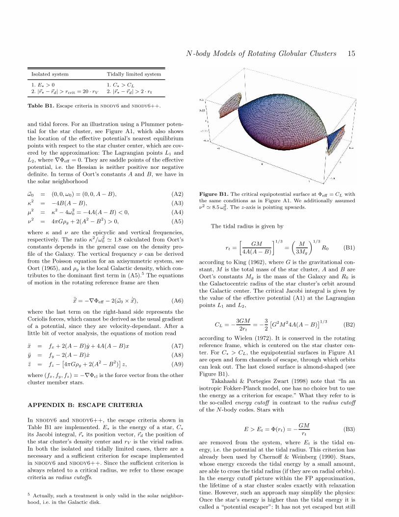
according to Wielen (1972). It is conserved in the rotatingreference frame, which is centered on the star cluster cen-ter. For C⋆ > CL, the equipotential surfaces in Figure A1are open and form channels of escape, through which orbitscan leak out. The last closed surface is almond-shaped (seeFigure B1).

Takahashi & Portegies Zwart (1998) note that “In anisotropic Fokker-Planck model, one has no choice but to usethe energy as a criterion for escape.” What they refer to isthe so-called energy cutoff in contrast to the radius cutoff

of the N-body codes. Stars with

E > Et = Φ(rt) = −GM

rt(B3)

are removed from the system, where Et is the tidal en-ergy, i.e. the potential at the tidal radius. This criterion hasalready been used by Chernoff & Weinberg (1990). Stars,whose energy exceeds the tidal energy by a small amount,are able to cross the tidal radius (if they are on radial orbits).In the energy cutoff picture within the FP approximation,the lifetime of a star cluster scales exactly with relaxationtime. However, such an approach may simplify the physics:Once the star’s energy is higher than the tidal energy it iscalled a “potential escaper”: It has not yet escaped but still

c© 2002 RAS, MNRAS 000, 1–16

16 A. Ernst, P. Glaschke, J. Fiestas, A. Just & R. Spurzem

Figure B2. Poincare section of orbits at the critical Jacobi in-tegral CL for the equations of motion (A7)-(A8) with the sameconditions as in Figure A1 at the moment of crossing y = 0 withy > 0. The full range of initial conditions is covered.

needs a time of the order of the crossing time to reach thetidal radius. Immediate removal of stars which fullfill theenergy criterion is only reasonable if the orbital timescale isnegligible compared with the relaxation time. An improvedapproach, which take this dependance on the crossing timescale into account, can be found in the paper by Lee & Os-triker (1987).

In an anisotropic FP code, it is possible to use the morerealistic apocentre criterion by Takahashi et al. (1997) andTakahashi & Portegies Zwart (1998): Stars are removed fromthe system, if their apocenter distance ra calculated accord-ing to

J2 = 2r2a [E − Φ(ra)] , (B4)

exceeds the tidal radius.Last but not least, in the case of a radius cutoff and

the tidal approximation, the picture is similar to the onesketched above: Once a star’s Jacobi integral C⋆ has ex-ceeded the critical value CL slightly (i.e. once the star isa “potential escaper”), it still needs a certain time to findan opening to one of the escape channels in the equipoten-tial surfaces shown in Figure A1 for the effective potential(A1). This can take many crossing times depending mainlyon the excess energy, i.e. we have te ∝ C2

L(C⋆ −CL)−2 from

an upper limit on the flux of phase space volume throughL1/L2 according to MacKay (1990) and Fukushige & Heggie(2000). In the radius cutoff picture within the tidal approx-imation, the scaling of the lifetime is very subtle and thehalf-mass time scales as tmh ∝ t

3/4rh , see Baumgardt (2001).

By integrating the equations of motion (A7) - (A9) nu-merically for orbits at a given Jacobi constant, one can ob-tain a Poincare section as shown in Figure B2. As seen inthis Figure, this is a system with divided phase space: Sev-eral “islands” of closed invariant curves in a stochastic “sea”show the existence of an additional conserved quantity otherthan the Jacobian for these orbits. The largest island ofquasiperiodic orbits in the left half of the surface of sectioncorresponds to retrograde orbits, i.e. the stars move aroundthe star cluster in the opposite sense to the motion of the star

cluster around the galaxy, see Fukushige & Heggie (2000).The “third integral” restricts their accessible phase spaceand hinders them from escaping, even if the stars have beenscattered above the critical Jacobi constant. On the otherhand, the particles on orbits corresponding to the chaoticdomains in the surface of section bounce back and forth fora certain time in a bounded area, called the “scattering re-gion”, until they escape through one of the exits, which openup around the Lagrangian points L1 and L2, for stars witha Jacobi constant, which is higher than the critical value.For an interesting overview of the physics of chaotic scatter-ing see the papers by Aguirre et al. (2001) and Aguirre &Sanjuan (2003).

This paper has been typeset from a TEX/ LATEX file preparedby the author.

c© 2002 RAS, MNRAS 000, 1–16