r/i;. HEWLETTa:~ PACKARD

On-Line Extraction of SCSI DiskDrive Parameters

Bruce L. Worthington*, Gregory R. Ganger*,Yale N. Patt*, John WilkesComputer Systems LaboratoryHPL-97-02January, 1997

E·mail: worthing, ganger, patt®eecs.umich.eduwilkes @hpl.hp.com

SCSI disk drives,parameters, automaticmeasurement

Sophisticated disk scheduling algorithms requireaccurate and detailed disk drive specifications,including information on mechanical delays, on­board caching and prefetching algorithms, commandprocessing and protocol overheads, and logical-to­physical block mappings. Comprehensive diskmodels used in storage subsystem design requiresimilar levels of detail. This report describes a suiteof general-purpose techniques and algorithms foracquiring the necessary data from SCSI disks via theANSI-standard interface. The accuracy of theextracted information is demonstrated by comparingthe behavior of a configurable disk simulator againstactual disk drive activity. Detailed measurementsextracted from several SCSI disk drives are provided.

* University ofMichigan, Ann Arbor, MichiganJointly published with the Department of Electrical Engineering and Computer Science at theUniversity ofMichigan as technical report CSE·TR·323·96, December 19, 1996.A condensed version of this report was published in the Proceedings of the 1995 ACMSIGMETRICS Joint International Conference on Measurement and Modeling of Computer Systems,Ottawa, Ontario, May 1995, pp.146-156.© Copyright Hewlett·Packard Company 1997

Internal Accession Date Only

TABLE OF CONTENTS

1 Introduction

2 Modern SCSI disk drives

2.1 Data layout .

2.2 Mechanical components

2.3 On-board controllers

2.4 On-board caches ..

2.5 Extraction complications.

3 Extraction environment

4 Interrogative extraction

4.1 Data layout parameters

4.1.1 READ DEFECT DATA

4.1.2 SEND/RECEIVE DIAGNOSTIC (TRANSLATE ADDRESS)

4.1.3 Notch Mode Page and READ CAPACITY .

5 Empirical extraction

5.1 Minimum time between request completions (MTBRC)

5.2 Test vector considerations

5.3 Seek curve .

5.4 Head switch and write settling times

5.5 Rotation speed . . . . . . . . . . . .

5.6 Command processing and completion overheads .

5.7 On-board caches .

5.7.1 Extraction example: discarding requested sectors after a READ

5.7.2 Extraction example: cache segments (number, type, and size)

5.7.3 Track-based vs. sector-based ....

5.7.4 Read-on-arrival and write-on-arrival

5.7.5 Segment allocation

5.7.6 Prefetch strategies

1

2

2

3

3

3

3

4

5

5

5

7

7

8

8

9

10

12

13

13

13

14

15

16

16

17

18

5.7.7 Buffer ratios

5.8 Path transfer rate.

6 Model validation

7 Use of extracted data in disk request schedulers

8 Conclusions

A Extraction algorithms

A.l Computing MTBRC values .

A.2 Command processing and completion overheads.

B Extracted parameters for specific disk models

B.l Seagate ST41601N

B.2 DEC RZ26

B.3 HP C2490A

B.4 HP C3323A

11

18

18

18

20

22

25

25

26

28

28

31

33

36

LIST OF FIGURES

1 Disk drive terminology.. 2

2 MTBRC example. ... 9

3 Seagate ST41601N: Extracted seek curves.. 11

4 Seagate ST41601N: Service time distributions.. 19

5 DEC RZ26: Service time distributions.. 19

6 HP C2490A: Service time distributions. 19

7 HP C3323A: Service time distributions. 19

8 Seagate ST41601N: Service time densities. 21

9 DEC RZ26: Service time densities. 21

10 HP C2490A: Service time densities.. 21

11 HP C3323A: Service time densities.. 21

12 Seagate ST41601N: Extracted seek curves.. 30

13 DEC RZ26: Extracted seek curves. . 32

14 HP C2490A: Extracted seek curves. 35

15 HP C3323A: Extracted seek curves. 38

111

LIST OF TABLES

1 Basic disk drive parameters. . . . . . . 5

2 Some relevant Mode Page parameters. 6

3 Seagate ST41501N: 50th percentile command processing and completion overheads. . 14

4 Seagate ST41601N: Basic disk drive parameters. 28

5 Seagate ST41601N: Zone specifications. . 28

6 Seagate ST41601N: Defect management. . 29

7 Seagate ST41601N: On-board cache characteristics. 29

8 Seagate ST41601N: 50th percentile command processing, completion, and mechanical overheads. 29

9 DEC RZ26: Basic disk drive parameters. . 31

10 DEC RZ26: Defect management. . . . . . 31

11 DEC RZ26: On-board cache characteristics. 31

12 DEC RZ26: 50th percentile command processing, completion, and mechanical overheads. 32

13 HP C2490A: Basic disk drive parameters. 33

14 HP C2490A: Zone specifications. . 33

15 HP C2490A: Defect management. . 34

16 HP C2490A: On-board cache characteristics. 34

17 HP C2490A: 50th percentile command processing, completion, and mechanical overheads. 34

18 HP C3323A: Basic disk drive parameters. 36

19 HP C3323A: Zone specifications. . 36

20 HP C3323A: Defect management. . 36

21 HP C3323A: On-board cache characteristics. 37

22 HP C3323A: 50th percentile command processing, completion, and mechanical overheads. 37

lV

(

1 Introduction

The magnetic disk drive remains firmly established as the preferred component for secondary data storage. Given

the growing disparity between processor and disk speeds, achieving high system performance requires that disk

drives be used intelligently. Previous work has demonstrated that aggressive disk request scheduling algorithms can

significantly reduce seek and rotational latency delays [Jacobson91, Seltzer90], and scheduling algorithmsthat exploit

on-board disk caches can further boost performance [Worthington94]. Such algorithms require detailed knowledge of

disk characteristics, including mechanical delays, on-board caching and prefetching algorithms, command processing

and protocol overheads, and logical-to-physical data block mappings. Accurate disk models utilized in storage

subsystem research require similar levels of detail [Ruemmler94].

Information about disk drives can be obtained by reading technical reference manuals, by directly monitoring

disk activity at the hardware level, or by talking directly to the drive firmware developers and mechanical engineers.

Unfortunately, disk technical manuals are typically incomplete and their accuracy is not guaranteed; direct obser­

vation requires expensive signal-tracing equipment and a great deal of time; and it is difficult to reach the correct

people at disk drive company XYZ and convince them to release what may be perceived as sensitive data. This

report explains how to extract the required information directly from on-line disk drives. In particular, it focuses on

disks that conform to the popular Small Computer Systems Interface [SCSI93].

In some cases, standard SCSI commands are used to request parameter values from the disk. These values are

typically static in nature, or nearly so. Although such interrogative extraction is convenient, it has two drawbacks:

(1) Because the ANSI standard allows a disk drive manufacturer to implement a subset of the full SCSI specification,

a given disk drive may not support all interrogative commands. (2) The parameter values returned may be inaccurate

or represent nominal figures, such as the mean number of sectors per track on a multi-zone disk.

In cases where interrogation cannot reliably obtain the necessary information, such as for timing-related pa­

rameters (e.g., seek times), the host can acquire the values by monitoring disk behavior at the device driver level.

Empirical extraction exercises a drive using carefully designed sequences of disk requests, or test vectors. Parameter

values are deduced from an analysis of the measured request service times. Much of this report is concerned with

the selection of appropriate test vectors that allow quick and accurate determination of parameter values despite the

complexity of modern SCSI disk drive controllers.

Depending on the purpose of the extraction, test vectors can be tuned for higher efficiency or greater precision.The default test vectors produce accurate parameter values within minutes. They can be reconfigured to execute in

considerably less time (e.g., a few seconds) at the cost of less reliable results. The extraction techniques have been

successfully applied to several SCSI disk drives, and accurate disk models have been configured with the measured

data. When using the extracted parameter values, detailed disk simulation closely matches real disk behavior.

The remainder of this report is organized as follows. Section 2 contains a brief description of modern SCSI disk

drives. For a more detailed discussion, the reader is referred to [Ruemmler94]. Section 3 identifies the system facilities

needed for parameter extraction and describes the experimental setup. Sections 4 and 5 describe interrogative and

empirical extraction techniques, respectively. Section 6 validates the extraction techniques. Section 7 discusses

how disk request schedulers can utilize extracted data. Section 8 contains concluding remarks and suggestions

for improving the process of disk characterization. The appendices provide additional detail on specific extraction

algorithms and list parameter values extracted from four different SCSI disk drives.

1

Arm

Read/Write Head--~~~~~~~~

Upper Surface --<Platter

Lower Surface --"\

Cylinder f---+-f-+--1

Sector---~~69:;::S:::::;'

Figure 1: Disk drive terminology.

2 Modern SCSI disk drives

2.1 Data layout

Actuator

A disk drive consists of a set of rapidly rotating platters (on a common axis) coated on both sides with magnetic

media (see figure 1). Data blocks on each surface are written in concentric tracks, which are divided into sectors. A

cylinder is a set of tracks (one from each surface) equidistant from the center of the disk. Longer tracks (i.e., those

farther out from the axis) can contain more data. To exploit this fact, the set of cylinders may be partitioned into

multiple zones or notches. (These two terms are used interchangeably throughout this report.) The number of sectors

per track increases from the innermost zone to the outermost zone.

Defects detected during the course of a disk's lifetime require data layout adjustments. Spare regions are reserved

to allow for defect slipping and reallocation. Sector (track) slipping takes place during disk formatting: the disk skips

over defective sectors (tracks) when initializing the data layout mapping. Each slipped region changes the mapping

of subsequent logical blocks. Defect reallocation (a.k.a. remapping or sparing) occurs when defective sectors are

discovered during normal disk use. The disk dynamically remaps affected data blocks to spare regions and redirects

subsequent accesses accordingly.

2

2.2 Mechanical components

A disk's read/write heads are held "over" a specific cylinder by a set of disk arms ganged together on a common

actuator. Most SCSI disks allow only one active read/write head at any given time. A seek moves the disk arms

to a new cylinder. Rotational latency denotes the time spent waiting for the target sector(s) to rotate around to

the active read/write head. Switching active heads may require a slight repositioning of the disk arms. The data

layout is designed to reduce the performance impact of such head switches on sequential transfers by offsetting the

logical-to-physical mapping between logically sequential tracks. The offset, or skew, prevents a request that crosses

a track or cylinder boundary from ''just missing" the next logical block and waiting almost a full rotation for it to

come around again.

2.3 On-board controllers

Modern SCSI disks use embedded controllers to decode and service SCSI commands. A host issues a request for

disk activity in terms of a starting logical block number (LBN) and a total request size. A disk controller maps the

simple linear address space of logical blocks into physical media locations. The details of servicing the request are

hidden from the host, ofHoading most of the management overhead associated with actual data storage from the host

(or intermediate I/O controller). As a result, entities outside of the drive typically have little or no knowledge of

the exact data layout, the status of the on-board disk cache, and the various overheads and delays associated with

servicing a disk request.

Some SCSI commands, such as MODE SENSE, MODE SELECT, and SEND/RECEIVE DIAGNOSTIC, allow access tocontrol and configuration information. If supported by the disk, they can be used during interrogative extraction.

Commands normally used to access data, such as READ and WRITE, can be used to empirically extract performance

characteristics.

2.4 On-board caches

Disk drives originally used on-board memory as a speed-matching buffer bet)'Veen media and bus transfers. Cur­

rent SCSI drives also use on-board memory as a data cache. On-board caches often contain multiple independentcache lines, or segments, to improve disk performance for workloads containing multiple interleaved sequential datastreams. A disk controller can automatically pre/etch data into a cache segment to reduce service times for subse­

quent sequential read requests. Disks with read-on-arrivalor write-on-arrival capability can transfer blocks between

the on-board cache and the magnetic media in the order they pass under the read/write head rather than in strictly

ascending LBN order.

2.5 Extraction complications

Disk behavior can appear unpredictable for many reasons, especially when compared against a simple model of

disk drive mechanics. Schemes for extracting detailed performance characteristics must cope with the complexities

3

of modern disk drives by circumventing certain disk controller optimizations. The extraction techniques discussed inthis report handle:

• overlapped disk controller overheads, SCSI bus data transfers, and mechanical delays

• contention for shared resources along the I/O path (e.g., buses and intermediate controllers)

• segmented on-board caches

• simple or aggressive prefetching algorithms

• non-uniform performance characteristics, such as actuator positioning algorithms optimized for very short seekdistances

• large, seemingly non-deterministic delays, such as those experienced during thermal recalibration

• minor fluctuations in timing

The existing extraction techniques must be augmented to handle disks with command queuing enabled (i.e., mul­

tiple commands queued at the disk). This is left as future work.

3 Extraction environment

The described extraction methodology requires a host computer system with direct, low-level SCSI access (by­

passing any file system or other translation/caching) and a high-resolution timer to measure the service times of

individual disk requests. Some systems (such as HP-UX [Clegg86]) have built-in trace-points that provide the neces­

sary timing capability. In other cases, the extraction techniques may require access to the OS source code, a device

driver development environment, or an I/O card that can be directly controlled by an application program (e.g., on

a machine running MS/DOS2).

The extraction experiments described in this report were performed using an NCR 3550 symmetric multiprocessor

running an MP-safe version of SVR4 UNIX3. Arbitrary SCSI commands were issued directly to specific disk drives

using a library of SCSI-related functions provided by NCR. To obtain fine-grained timing data, the device driverwas modified to measure service times using a diagnostic counter with a resolution of 840 nanoseconds. Extraneous

activity on the host system was minimized to reduce extraction time. Although the algorithms produce valid results

in the presence of timing noise (e.g., additional CPU load and bus contention), they take longer to do so.

The extraction techniques were developed and tested using four different disk drives: a Seagate ST41601N[Seagate92, Seagate92a], a DEC RZ26, an HP C2490A [HP93], and an HP C3323A [HP94]. Table 1 lists some basic

characteristics of these drives.

2MS/DOS is a registered trademark of Microsoft Corporation.3UNIX is a registered trademark of X/Open Corporation.

4

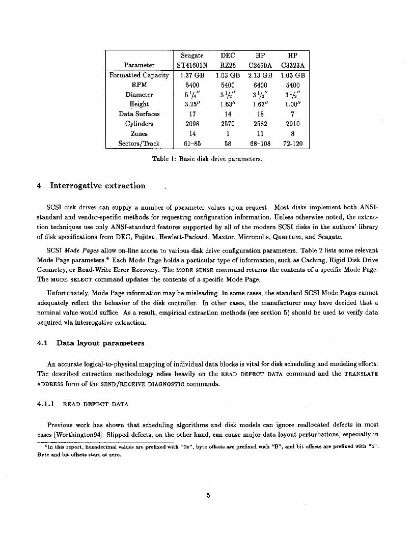
Seagate DEC HP HP

Parameter ST41601N RZ26 C2490A C3323A

Formatted Capacity 1.37 GB 1.03 GB 2.13 GB 1.05 GB

RPM 5400 5400 6400 5400Diameter 5 1

/ 4 " 3 112" 3 112" 3%"Height 3.25" 1.63" 1.63" 1.00"

Data Surfaces 17 14 18 7Cylinders 2098 2570 2582 2910

Zones 14 1 11 8

Sectors/Track 61-85 58 68-108 72-120

Table 1: Basic disk drive parameters.

4 Interrogative extraction

SCSI disk drives can supply a number of parameter values upon request. Most disks implement both ANSI­

standard and vendor-specific methods for requesting configuration information. Unless otherwise noted, the extrac­

tion techniques use only ANSI-standard features supported by all of the modern SCSI disks in the authors' library

of disk specifications from DEC, Fujitsu, Hewlett-Packard, Maxtor, Micropolis, Quantum, and Seagate.

SCSI Mode Pages allow on-line access to various disk drive configuration parameters. Table 2 lists some relevant

Mode Page parameters.4 Each Mode Page holds a particular type of information, such as Caching, Rigid Disk Drive

Geometry, or Read-Write Error Recovery. The MODE SENSE command returns the contents of a specific Mode Page.

The MODE SELECT command updates the contents of a specific Mode Page.

Unfortunately, Mode Page information may be misleading. In some cases, the standard SCSI Mode Pages cannot

adequately reflect the behavior of the disk controller. In other cases, the manufacturer may have decided that a

nominal value would suffice. As a result, empirical extraction methods (see section 5) should be used to verify data

acquired via interrogative extraction.

4.1 Data layout parameters

An accurate logical-to-physical mapping of individual data blocks is vital for disk scheduling and modeling efforts.

The described extraction methodology relies heavily on the READ DEFECT DATA command and the TRANSLATE

ADDRESS form of the SEND /RECEIVE DIAGNOSTIC commands.

4.1.1 READ DEFECT DATA

Previous work has shown that scheduling algorithms and disk models can ignore reallocated defects in most

cases [Worthington94]. Slipped defects, on the other hand, can cause major data layout perturbations, especially in

4In this report, hexadeciIIUll values are prefixed with "Ox", byte offsets are prefixed with "B", and bit offsets are prefixed with "b".

Byte and bit offsets start at zero.

5

I Location IDisconnect-Reconnect (Ox02)

Buffer Full Ratio B2Buffer Empty Ratio B3

Bus Inactivity Limit B4-B5

Disconnect Time Limit B6-B7

Connect Time Limit B8-B9Maximum Burst Size BIO-BllData Transfer Disconnect Control B12bO-bl

Format Device (Ox03)Tracks Per Zonead B2-B3Alternate Sectors Per Zonead B4-B5Alternate Tracks Per Zonead B6-B7

Alternate Tracks Per Logical Unita B8-B9

Sectors Per Tracka BIO-Bll

Data Bytes Per Physical Sectora B12-B13Interleaveab B14-B15Track Skew Factora B16-B17Cylinder Skew Factora B18-B19Surface Modec B20b4

Rigid Disk Geometry (Ox04)

Number of Heads B5

Medium Rotation Rate B20-B2I

Caching (Ox08)Read Cache Disable B2bOMultiplication Factor B2bIWrite Cache Enablec B2b2Disable Prefetch Transfer Length B4-B5Minimum Prefetch B6-B7Maximum Prefetch B8-B9Maximum Prefetch Ceiling BIO-Bll

Notch (OxOC)

Logical Or Physical Notcha B2b6Maximum Number of Notches B4-B5Active Notch B6-B7Starting Boundarya B8-BllEnding Boundarya B12-B15

I Mode Page & Parameter

" Active Notch must be set via Mode Select before requesting per-notch values.

b Must be zero or one during extraction.

C Must be zero during extraction.

d For this parameter, "Zone" refers to a region over which spare sectors are allocated. In

other contexts, "Zone" is a common synonym for "Notch."

Table 2: Some relevant Mode Page parameters.

6

the case of track-based slipping. As reallocated defects may be converted into slipped defects during disk format,

data layout extraction should be repeated after reformatting. The READ DEFECT DATA command requests a list of

defective sectors (or tracks) from a disk in cylinder/head/sector (or cylinder/head) format. To obtain a complete

list of all defects detected during and after manufacture, both the Primary Defect List Bit (B2b4) and Grown Defect

List Bit (B2b3) must be set in the READ DEFECT DATA command descriptor block.

4.1.2 SEND/RECEIVE DIAGNOSTIC (TRANSLATE ADDRESS)

The TRANSLATE ADDRESS form of the SEND DIAGNOSTIC command requests the exact logical-to-physical map­

ping for a single logical block. The corresponding physical media location (cylinder/head/sector) is returned by a

subsequent RECEIVE DIAGNOSTIC command. Obtaining a fulllogical-to-physical mapping by iterating through every

logical block number can take several hours. A variety of shortcuts are used to reduce the number of SEND /RECEIVE

DIAGNOSTIC command pairs required to obtain a complete mapping. The extraction algorithms first determine theboundaries, sectors per track, track skew, and cylinder skew for each zone, or verify this information if it was obtained

from the Mode Pages. The current mapping is then requested for the "expected" first and last logical block of eachcylinder. Alternately, a faster algorithm might examine only a fraction of the total set of cylinders. Mismatches

between actual and expected values indicate the existence of slipped defects or spare regions, which can then bepinpointed with additional SEND/RECEIVE DIAGNOSTIC command pairs in a binary search pattern.

4.1.3 Notch Mode Page and READ CAPACITY

Unfortunately, there is at least one major disk manufacturer, Quantum, that does not always provide TRANSLATE

ADDRESS functionality. For drives lacking this capability, an alternate methodology for extracting data layoutinformation is required. In the specific 'case of Quantum disk drives, many of the necessary parameter values can be

obtained using the Notch Mode Page and the READ CAPACITY command.

When a disk supports both the Notch Mode Page and the Format Device Mode Page (see table 2), it is possible to

obtain most of the necessary mapping information using the Mode Select command. The combination of parameter

values from these two pages specifies the data layout and size of each notch. The READ CAPACITY command can

be used to determine the logical boundaries of each cylinder, provided that the implementation of the command

allows for the retrieval of individual cylinder capacities. This information can be used to identify deviations fromthe per-notch Mode Page parameter values. Additional empirical extraction is still necessary to validate the ModePage parameter values as well as to obtain data layout information that cannot be interrogatively extracted withoutTRANSLATE ADDRESS functionality. For example, the skew between the last sector of a given notch and the first sector

of the next notch is not specified by any Mode Page field. Also, not all defect-handling schemes can be adequately

represented using the fields of the Format Device Mode Page.

Complete details of the alternate data layout extraction methodology using the Notch Mode Page and READ

CAPACITY command are not included in this report.

7

5 Empirical extraction

Although some disk parameters and characteristics can be obtained via interrogation, many must be deduced

by observing dynamic disk behavior. This section describes various empirical extraction algorithms and their use in

measuring disk performance characteristics. In particular, it contains descriptions of a general empirical extraction

methodology, algorithms for extracting mechanical parameter values, algorithms for approximating command pro­

cessing and completion overheads, techniques for characterizing cache behavior, and a simple algorithm for computing

an overall I/O path transfer rate.

For modeling purposes, mean or 50th percentile parameter values are often sufficient. For other purposes,

(probabilistic) upper bound values may be necessary. For example, a disk request scheduler configured with mean

values will frequently underpredict command processing overheads and mechanical positioning times, occasionally

resulting in excessive rotational delays. It may be advantageous to use conservative parameter values instead, limiting

the opportunity for unacceptable delays. For this reason, maximum or 95th percentile values are also extracted.

5.1 Minimum time between request completions (MTBRC)

Many of the empirical extraction techniques rely on measuring the minimum time between request completions

for specific pairs of request types. MTBRC(X,Y) denotes the minimum time between the completions of a request of

type X and a request of type Y. For example, MTBRC(I-sector write, I-sector read on an adjacent cylinder) refers

to the minimum time between request completions for a I-sector write request followed by a I-sector read request

requiring a I-cylinder seek.

The determination of an accurate MTBRC value is an iterative process, wherein the inter-request distance between

each pair of requests (i.e., between each type X and type Y request) is varied until the minimum time between request

completions is observed. The inter-request distance is the rotational distance between the physical starting locations

of each MTBRC request pair, measured along the direction of rotation. When the X requests are for small amounts

of data and the Y requests do not incur significant seek times, inter-request distances are only a fraction of a full

rotation. So, for example, MTBRC(I-sector write, I-sector read on the same track) might have a corresponding

inter-request distance of 25 sectors, given a fixed number of sectors per track. Assuming sectors 100 and 125 are on

the same track, the minimum time between request completions would be observed for a I-sector write to sector 100

followed by a I-sector read from sector 125. If the number of sectors per track varies across the disk, then the inter­

request distance can be measured as the angle between the first sectors of the request pairs, or as the time necessary

for the disk to rotate through this angle. Appendix A.I provides a detailed algorithm for extracting MTBRC values.

To determine the MTBRC for a given request pair specification, the iterative MTBRC algorithm finds the inter­

request distance for which the second request of each pair incurs essentially zero rotational latency. Any rotational

latency that is not in parallel with command processing overheads or mechanical delays must be less than the time

necessary to rotate past one sector of data. Otherwise, a shorter inter-request distance would result in a lower time

between request completions.

The algorithm also computes the mean host delay. The host delay is the time between the completion of the first

request of a request pair and the initiation of the second request. This delay is due solely to processing time at the

host (e.g., executing device driver code, configuring intermediate controllers, and copying data from kernel memory

8

... MTBRC --------......1

~------- Request 1 --------i..~1 1~4...----- Request 2 -----_..~I

Track EndTrack Start

com-I SeekIRotational I Media I Bus I Com- Host com-I Rotational IMedia I Bus I Com­mand Latency Access Transfer pletion Delay mand Latency Access Transfer pletion

I , "', II , , ,I I , ,I , , ,

L...-__•__·_·__---JDse~tori~... •__·_· ....JC§;.---T"""-·--·--.-I.. Inter-Request Distance = X ----....... 11

TIME

Figure 2: MTBRC example. The time-line shows the service time components for an example MTBRC(I-sector READ,

I-sector READ on same track) request pair. The track accessed by the two requests is also shown, but as a straight line ratherthan as a circle. Timestamps are taken at the initiation and completion of each request, providing the host delay and theMTBRC timings. The inter-request distance is the difference between the starting locations of the two requests.

to user space). Mean host delays can be subtracted from MTBRC values to remove variations in host processing

times. Figure 2 shows the service time components for an example MTBRC request pair.

In order to determine a value for a specific disk parameter, MTBRC values are collected for two or more sets

of selected request type pairs. Each MTBRC value is the sum of several discrete service time components. Specific

component values are isolated via simple algebraic techniques. In section 5.4, for example, the effective head switch

time is computed from MTBRCI (1-sector write, 1-sector read on the same track) and MTBRC2 (1-sector write,

1-sector read on a different track of the same cylinder). The corresponding equations are:

MTBRCI = HostDelaYI + Command + Media + Bus + Completion

MTBRC2 = HostDelaY2 + Command + HeadSwitch + Media + Bus + Completion

Via substitution and reorganization:

HeadSwitch = (MTBRC2 - HostDelaY2) - (MTBRCI - HostDelaYI)

5.2 Test vector considerations

Empirical extraction test vectors range from tens to thousands of requests in length. In many cases, a large

fraction of the requests are intended to defeat controller optimizations and eccentricities. Test vectors must be

carefully designed to prevent unexpected mechanical delays and/or interference from the on-board cache, even when

the cache is only functioning as a speed-matching buffer:

• As some disks must "warm-up" after they have been idle for some period of time, each test vector is prefixed by

20-50 random disk requests whose service time measurements are discarded. Without this precaution, the first

10-20 requests of a test vector can take up to ten times longer than normal to complete.

9

• Anyon-board write-back (a.k.a. fast-write) cache activity should be disabled during extraction by setting theWrite Cache Enable Bit to zero (see table 2).

• When it is necessary to force cache misses for READ requests, the cache must be appropriately initialized. If

the cache uses a Least Recently Used (LRU) segment replacement algorithm, for example, initialization involves

issuing a number of physically scattered READs equal to the maximum number of cache segments.

• As read requests often invoke automatic prefetching activity that may result in unwanted switching between

tracks (or cylinders), test vectors should use WRITE requests or choose initial MTBRC READ targets from the

lowest LBNs on a track. The latter option relies on host delay values being short enough and/or rotation speeds

being slow enough to allow any positioning activity for the second request to be initiated before the logical end

of the current track is reached.

• The overlap between media and bus transfers can be eliminated by using I-sector requests or by setting the Buffer

Ratio fields (see table 2) to values that minimize data transfer pipelining, provided that the disk controller obeys

these values. Specifically, a large Buffer Full Ratio will cause the disk controller to wait for all READ data to

be cached before reconnecting to the bus. It is more difficult to prevent overlap between WRITE data transfer

and media access. If multi-sector WRITE requests are required, they should be designed to incur long mechanical

delays, thereby increasing the probability that all data transfer over the bus is completed prior to any media

access.

5.3 Seek curve

A seek curve graph displays seek time as a function of seek distance. The seek time between two cylinders

is a complex function of the position of the cylinders (i.e., their distance from the spindle), the direction of the

seek (inward or outward), various environmental factors (e.g., vibration and thermal variation), the type of servo

information (dedicated, embedded, or hybrid), the mass and flexibility of the head-arm assembly, the current available

to the actuator, etc. A seek curve attempts to reduce this complexity into a single mapping of seek distances to seek

times.

Different algorithms may be used for extracting seek curves depending on whether the end goal is accurate disk

modeling or high-performance disk request scheduling. A disk model should use a seek curve that reflects mean seek

times for each seek distance. A mean seek curve may be inexact for any given request, but it should result in a good

overall emulation of seek behavior. A disk scheduler, on the other hand, may be better served by a more conservative

seek curve containing near-maximum seek times.

The following algorithm extracts two seek curves. It requires an accurate logical-to-physical map (see section 4.1)

and the use of the SEEK command. The first seek curve consists of mean seek times for specific seek distances. The

second curve, denoted as the "maximum" seek curve, gives an approximate upper bound on seek times for the same

set of seek distances.

1. For each seek time to be extracted, select 5 starting points evenly spaced across the physical cylinders. For longer

seek distances, the number of starting points may be decreased. Full stroke seeks, for example, must necessarily

start on either the innermost or outermost cylinder. From each starting point, perform 10 inward and 10 outward

SEEKs of the appropriate distance. While most of the measured service times should be roughly equivalent, there

will often be anomalous values caused by non-deterministic disk activity (e.g., thermal recalibration or mis-reads),

periodic host activity (e.g., clock interrupts), or unexpected contention for other shared resources (e.g., SCSI

10

20

5

-Maximum--_. Mean

6

5

Ci)'~4Q)

.§f.;;:3

1 ,/(/) 2 I

II

II

I

~,;"",,

-Maximum--- Mean

o..l---_r_-~___r-~-_r_--_r_-~___r-500 1000 1500 2000

Seek Distance (Cylinders)

(a) Full seek curve

20 40 60 80Seek Distance (Cylinders)

(b) Expanded view of short seeks

100

Figure 3: Seagate ST41601N: Extracted seek curves.

bus traffic involving other disks). Excessive service times may be omitted if such activities are to be ignored by

the disk model or scheduler. For the seek curves given in this report, service times deviating from the median

value by more than 10% were discarded.

2. Average the 5 sets of measured service times to obtain a single mean service time value for each of the 5 starting

points.

3. For the mean seek curve, average the 5 mean service time values. For the maximum seek curve, take the maximum

of the 5 values. Thus the maximum seek curve extracted by this algorithm reflects mean seek times for regions of

the disk which generally experience the longest seek times. If tighter guarantees on response times are desired,

other algorithms might be more appropriate. For example, 95th percentile values could be computed for each of

the 5 sets of measured service times, and the maximum seek curve could be comprised of the maximums of the95th percentile values. Alternately, partial seek curves could be extracted for different regions of the disk.

4. After the mean and maximum service times have been determined for each seek distance, the portion of the

service time due to actuator movement must be isolated. A corrective value is computed from MTBRC(l-sector

write, I-sector read on the same track) and MTBRC(I-sector write, I-sector read on an adjacent cylinder). The

difference between these two values effecti"ely represents the time necessary to mechanically seek across one

cylinder. The difference between this value and the extracted l~cylinder SEEK service time represents the non­

mechanical overheads associated with processing a SEEK request. This processing delay should be subtracted

from each extracted service time. The resulting values comprise the extracted mean and maximum seek curves.

Figure 3 shows the extracted seek curves for a Seagate ST41601N. As the seek distance increases, seek curves

become linear. In fact, most seek times for larger seek distances can be computed using linear interpolation, thereby

reducing the number of actual measurements necessary. The seek curves in figure 3 contain seek times for every seek

11

distance between 1 and 10 cylinders, every 2nd distance up to 20 cylinders, every 5th distance up to 50 cylinders,every 10th distance up to 100 cylinders, every 25th distance up to 500 cylinders, and every 100th seek distance

beyond 500 cylinders. Using this method, the extraction process takes less than two minutes for each of the four

disks tested. By reducing the number of starting points, repetitions, and/or measured seek distances, the extraction

time can be reduced with some loss of accuracy.

5.4 Head switch and write settling times

The time necessary to switch read/write heads depends primarily on the type of servo information utilized by

the disk drive (dedicated, embedded, or hybrid) and various environmental factors, such as vibration and thermal

variation. For the current generation of disk drives, any seek activity will typically subsume the head switch time.

WRITE requests incurring head switches or seeks may require additional settling time to more closely align the

read/write heads. Data can be read from the media successfully even when the read/write heads are slightly

misaligned, but data must be written as close to the middle of a track as possible in order to prevent corruption

of adjacent tracks of data. So, the time necessary to position the actuator and activate the appropriate read/write

head is calculated as follows:

ActuatorPrepSeek = Seek (+WriteSettle if WRITE)

ActuatorPrepNoSeek = H eadSwitch (+W riteSettle if WRITE)

Since head switch and write settling times ca~not be measured directly, the extraction algorithms compute effective

values that are sufficient for disk modeling and request scheduling purposes.

The effective head switch time is the portion of the head switch time that is not overlapped with command

processing or data transfer. It can be computed from MTBRC1 (1-sector write, I-sector read on the same track) and

MTBRC2(1-sector write, I-sector read on a different track of the same cylinder), as described in section 5.1:

HeadSwitch = (MTBRC2 - HostDelaY2) - (MTBRC1 - HostDelayd

The effective write settling time is the portion of the write settling time that is not overlapped with command

processing or data transfer. It can be computed from the effective head switch time, MTBRC1(I-sector write, I-sector

write on same track), and MTBRC2 (1-sector write, I-sector write on a different track of the same cylinder):

WriteSettle = ((MTBRC2 - HostDelaY2) - (MTBRC1 - HostDelayd) - HeadSwitch

The difference between the two MTBRC values (after accounting for any difference in mean host delays) is the sum of

the effective head switch and effective write settling times. The effective write settling time is isolated by subtractingout the effective head switch time. Negative effective write settling times were computed for some of the disks tested,

indicating that additional overlap occurs between head switching/write settling and command processing/bus transfer

for WRITEs. A negative effective write settling time poses no problem as long as the overall actuator positioning

and head switch delay (ActuatorPrep) is positive. For disks using only dedicated servo information, such as the

Seagate ST41601N, the extracted effective head switch and same-cylinder write settling times may be negligible. But

write settling is still a factor for requests that incur seek activity. An effective "seek-only" write settling time can

12

be computed for such disks by modifying the above algorithm to use MTBRC2(I-sector write, I-sector write on an

adjacent cylinder).

Track skew can be used as a high-probability upper bound on the combined head switch and write settling delays.

Disk manufacturers set track skew values to minimize the interruption in media access incurred when sequentialtransfers cross track boundaries.

5.5 Rotation speed

Rotation speed can be determined empirically by performing a series of I-sector WRITEs to the same location and

calculating the mean time between request completions. A small number of repetitions (e.g., 32) should be sufficient

to obtain an accurate value. The mean time between completions is equal to the time per rotation, which is the

reciprocal of rotation speed. Extracted rotation speeds for the four disks tested are within manufacturer-specified

tolerances.

5.6 Command processing and completion overheads

Given a "black-box" extraction methodology, it is difficult to measure certain parameters directly. Command

processing, completion, and other overheads can only be measured as combined quantities unless the extraction

process has access to timing information for when actual data transfers begin and end. Command processing and

completion overheads can depend on the type of command (READ or WRITE), the state of the cache (hit or miss),

and the immediately previous request's characteristics [Worthington94]. Overhead values can be approximated by

solving multiple linear equations obtained from MTBRC extractions for the various unknown values. For disk models,

the level of detail desired determines the number of different MTBRC extractions necessary. For disk schedulers,

combined quantities can be used directly (see section 7).

To configure a disk simulator for validation purposes (see section 6), ten equations containing eight unknowns (six

command processing overheads and two completion overheads) were solved for each of the four disks tested. When

inconsistent equations suggested conflicting values for an overhead, the mean of the conflicting values was used. It

was also necessary to reduce the number of unknowns by arbitrarily setting one unknown to zero (see section A.2).

Table 3 shows extracted and published overhead values for the Seagate disk drive. Note the significant variationbetween processing overhead values for different types of commands. The difference between extracted and published

values is due in part to the fact that extracted values include some host delay, SCSI protocol overhead, and concurrent

mechanical activity.

5.7 On-board caches

The standard SCSI specification provides for a wide range of cache-management policies, and manufacturers

are free to extend this range. This section discusses a methodology for characterizing on-board disk caches. The

methodology consists of a series of experiments (i.e., test vectors) that prove or disprove specific hypotheses about

cache behavior. Boolean parameter values (e.g., can a READ hit on cached data from a previous WRITE?) typically

require only one test vector. Tests for cache parameters that can take on several values (e.g., the number of cache

13

Overhead Value

Read Hit After Read 0.895 msRead Hit After Write 0.497 ms

Read Miss After Read 1.442 ms

Read Miss After Write 1.442 ms

Write After Read 2.006 ms

Write After Write 1.473 ms

Read Completion 0.239 ms

Write Completion 0.000 ms

Published Per-Command 0.700 ms

Table 3: Seagate ST41501N: 50th percentile command processing and completion overheads.

segments) use feedback from each hypothesis to help select the next hypothesis and test vector. Designing a complete

set of hypotheses is difficult, if not impossible; the on-board cache can only be characterized to the extent ofthe extraction algorithms' knowledge of possible cache characteristics. The current suite of extraction algorithmssuccessfully characterized the cache behavior of the four disks tested.

Algorithms that extract cache parameter values generally contain three phases: (1) A hypothesis about cache

behavior is made. (2) The cache is loaded with data through the issuing of one or more specific disk requests. (3) The

contents of the cache are inspected by issuing a single READ request and determining whether or not the request hit

in the on-board cache. The requests issued in phases two and three comprise a test vector.

The following sections give several examples to demonstrate this extraction technique and discuss the types of

parameters that characterize an on-board disk cache.

5.7.1 Extraction example: discarding requested sectors after a READ

Some on-board cache management algorithms give precedence to prefetched data over requested data. Such

algorithms assume that subsequent requests are more likely to access sequential data than previously requested data.

This optimization can be implemented in several different ways. Prefetching activity may "push" requested data

out of a cache segment once the segment is full, thereby allowing additional sectors to be prefetched. Alternately,

requested sectors can be discarded from the cache as soon as they are transferred to the host, leaving the entire

segment available for prefetching activity. The following algorithm tests for the latter option.

Choosing the hypothesis

1. Assume that sectors requested by a READ are discarded from the cache before the request is considered complete.

Loading the cache

2. Perform a I-sector READ of a randomly-chosen logical block.

14

Testing the hypothesis

3. Perform a I-sector READ of the same logical block. The request should incur almost a full rotation of latency,

since the requested sector should no longer exist in the on-board cache. A request response time in excess

of 3/4 of a rotation should be sufficient indication that a cache miss occurred, assuming that completion and

cleanup, host, and protocol delays take up less time than 1/4 of a rotation.

If the second request completes in less than 3/4 of a rotation, a cache hit has occurred, the test has failed, and

it can be assumed that the target sectors of a READ request remain in the on-board cache after the request hascompleted.

5.7.2 Extraction example: cache segments (number, type, and size)

Although modern SCSI disk drives typically contain Mode Page data regarding the characteristics of on-boardcache segments, such information is not required or well-specified by the ANSI standard. For this reason, empirical

extraction techniques are necessary to obtain or validate cache segment configuration and management data.

The following algorithm determines the maximum number of cache segments available to READs:

Choosing the initial hypothesis

1. Set N, the hypothesized number of READ segments, to a large value (e.g., 32).

Loading the cache

2. Perform I-sector READs of the first logical blocks of the first N-l data cylinders. By only accessing blocks that

are at the logical "beginnings" of their respective cylinders, the possibility of unwanted head switchs and seeks

caused by automated prefetching activity is minimized (see section 5.2).

3. Perform a I-sector READ of the first logical block of the last data cylinder. This will cause the next request to

incur a full-stroke seek.

Testing the hypothesis

4. Perform a I-sector READ of the first logical block of the first data cylinder. A cache hit should occur if the

number of cache segments is N or greater, assuming a segment replacement scheme such as LRU or FIFO. Arequest response time of less than 3/4 of a rotation should be sufficient indication that a cache hit occurred,assuming that a full-stroke seek takes more than 3/4 of a rotation.

Choosing the next hypothesis

5. If step 4 results in a cache miss, the test has failed. Decrement N and return to step 2. If step 4 results in acache hit, the test has succeeded and the cache has at least N READ segments. If N is the largest hypothesized

value that has been tested, increment N and return to step 2. Otherwise, there are exactly N READ segments.

To increase the algorithm efficiency, a standard binary search can be employed.

This algorithm is designed for caches with multiple segments. The existence of a single cache segment can be

detected by issuing two I-sector READs for the same location and determining whether or not the second READ hits

in the cache. If the second request misses, it will incur almost a full rotation of latency. A request response time in

15

excess of 3/4 of a rotation should be sufficient indication that a cache miss occurred, assuming that completion and

cleanup, host, and protocol delays take up less time than 1/4 of a rotation. If no segments are detected, the first

algorithm should be repeated with step 4 modified to read the second logical block from the first data cylinder. This

will handle disks that discard requested data after completing a READ (see section 5.7.1). It assumes that each of

the requests result in a small amount of automated prefetching activity before the servicing of the next request.

Some on-board caches have dedicated segments for use by WRITES, while others allow all segments to be used by

READs or WRITES. Additional test vectors can determine which scheme has been implemented. For example, steps 2

and 3 can be modified to include one or more WRITEs. If the extracted number of cache segments increases, one or

more cache segments are dedicated to WRITEs. If the extracted number of segments remains unchanged, some or all

of the segments are usable by either READs or WRITEs.

Extracting the size of the cache segments can be quite simple or very difficult depending on the prefetching

behavior of the disk. The basic extraction technique computes the segment size by filling a cache segment with data

(e.g., via a large READ) and then determining the boundaries of the segment by detecting READ hits (or misses) against

the cached data. Sufficient time is allowed for all prefetching activity to cease before probing the segment boundaries

with I-sector READ requests. Of course, the cache segment must be re-initialized after each "probe" request, as

READ misses or additional prefetching may change the segment contents. The most difficult scenario involves disks

that discard requested sectors after they are transferred to the host (see section 5.7.1). If the subsequent prefetching

activity halts before filling the segment, the extraction algorithm may underestimate the size of the cache segments.

For such disks, an attempt must first be made to maximize the prefetching activity by changing the appropriate

Mode Page parameters (see table 2).

Some disks dynamically modify the number (and size) of cache segments based on recent request patterns. It

may be difficult to accurately characterize the on-board caching behavior of such disks.

5.7.3 Track-based vs. sector-based

Some on-board caches allocate space (i.e., segments) based on track size. This has obvious implications for

disks with zoned recording: assuming that the cache segments are the size of the largest track, cache space will

be underutilized when sectors from smaller tracks are stored in the cache. Track-based caches can be detected by

issuing large read requests, allowing prefetch activity to subside, and then determining the contents of the cache, in

a manner similar to the extraction of cache segment size (see section 5.7.2). If the range of cached sectors always

starts on a track boundary, the odds are fairly high that the cache is track-based. Other potential indicators of

track-based caching are prefetching algorithms that stop on track boundaries and segment sizes that appear to be

an exact multiple of the current zone's track size.

5.7.4 Read-on-arrival and write-on-arrival

Track-based and aggressive sector-based caches can process disk sectors in the order they pass under the read/write

head rather than in strictly ascending LBN order. Write-on-arrival can be detected by writing a I-sector request

to the first logical block of a track followed by a track-sized write request starting at the same logical block. If the

disk does not have write-on-arrival capability, the request should take approximately two rotations to complete: one

rotation to reach the starting block location and one rotation to write the data. With write-on-arrival capability,

16

the request should be serviced in much less than two rotations, as it can begin writing sectors to the disk media as

soon as they are transferred to the on-board cache. Note that this assumes a path transfer rate that is faster than

the media access rate. Choosing a logical track near the spindle will increase the path:media transfer ratio. If the

path transfer rate is still too slow, alternate test vectors can be devised. For example, smaller write requests can be

used to reduce the possibility of additional rotational delays caused by emptying the on-board cache segment.

Read-on-arrival may apply specifically to requested sectors or to non-requested sectors or to both. To test for

this capability, issue a I-sector read request to sector N, the last logical sector on a specific track. Immediately issue

a I-sector read request to sector N-l. Repeat this sequence several times selecting different values for N. If the disk

allows read-on-arrival for non-requested sectors, the second request of each pair s~ould almost always hit in the cache.

Read-on-arrival for requested sectors is detected by issuing a I-sector read request followed by a full-track read request

to another track on the same cylinder as the first request. The two requests should be physically aligned (i.e., they

should start at the same rotational position). Upon decoding the second request, the disk activates the appropriate

read/write head and performs any necessary actuator fine-tuning. Without read-on-arrival capability, the disk then

waits for the first target sector to rotate all the way around to the read/write head. A disk using read-on-arrival, on

the other hand, immediately begins reading requested sectors after the head switch is complete. Given knowledge

of the path transfer rate, the media transfer rate, and the disconnection behavior (e.g, by preventing disconnection

via the Disconnect Privilege Bit of the Identify Message), the rotational latency incurred can be deduced, and thus

read-on-arrival capability can be detected.

5.7.5 Segment allocation

There are many issues regarding the allocation of cache segments. Segments mayor may not be partitioned

between READ data and WRITE data (see section 5.7.2). Read requests mayor may not be able to hit on data placed

in the cache by write requests. When it becomes necessary to assign a "new" segment, the origin of the data in each

existing segment (READ, WRITE, or prefetch) may be considered, or a simple allocation policy such as LRU may be

employed. When a write request includes sectors that are already present in the on-board cache, the disk must make

sure that "old" sectors are invalidated. The timing and extent of such invalidation varies. For example, the entire

cache can be invalidated on every WRITE, or just segments with overlapping sectors can be invalided, or just the

overlapping sectors can be invalidated.

For track-based caches, a pair of track-sized segments may be assigned to each request, allowing a "ping-pong"behavior where the media access uses one segment (track) while the bus access uses the other. This may cause

significant confusion during extraction, especially in conjunction with track-based prefetching algorithms, unless the

extraction methodology specifically tests and accounts for this scenario.

Although these issues are complex, each segment allocation characteristic may be tested for using the hypothesis­

and-test methodology. In each case, the extraction program or user makes an assumption (e.g., that READs can hit

on WRITE data) and sets up the cache to allow detection of a read hit or miss (e.g., a test vector with a write request

followed by a read request for the same data).

17

5.7.6 Prefetch strategies

Table 2 includes several prefetch parameters obtainable from the Mode Pages. For example, the amount of

prefetched data may be linked to the size of the READ request that preceded the prefetching activity, as is the case

when the Multiplication Factor Bit on the Caching Mode Page is set to one. Other prefetch characteristics can only

be empirically determined, such as whether or not prefetching activity can traverse track or cylinder boundaries and

what happens when the cache segment fills up during prefetch. By issuing different sequences of requests and testing

the resulting contents of the cache (i.e., hypothesis and test), various prefetch strategies can be detected.

5.7.7 Buffer ratios

The Buffer Full Ratio and Buffer Empty Ratio values specified on the Disconnect-Reconnect Mode Page are

required for comprehensive disk modeling. They indicate how full a read cache segment should be and how empty

a write cache segment should be before the disk attempts reconnection to the host. However, some disks utilize

adaptive algorithms when these values are set to OxOO [HP93, HP94]. To determine if this is the case, set the Buffer

Full Ratio to OxOO and compute MTBRC(l-sector write, segment-sized read) for the outermost zone. Repeat the

extraction with Buffer Full Ratio set to OxOl. If the OxOO MTBRC is significantly different from the OxOI MTBRC

(i.e., the OxOO case is attempting to utilize bus resources more efficiently), an adaptive algorithm may be in use.

5.8 Path transfer rate

The data transfer rate between a disk and main memory is a function of the sustainable bandwidth of each

component in the I/O data path (e.g., main memory, controllers, buses, adapters, and disk). A single value for the

path transfer rate can be determined by comparing service times for two different-sized READ requests that hit in the

on-board disk cache. Since the media is not accessed for a READ hit, the only difference between the service times is

the additional path transfer time for the larger request.

6 Model validation

To validate the described extraction methodology, parameter values were extracted from four different disk

drives (see table 1). A detailed disk simulator was configured with the extracted values to allow comparison between

measured and modeled disk behavior. In each case, the mean service time reported by the simulator was within 1% of

the value observed for the actual disk (servicing the same workload).

Greater insight can be achieved by comparing the service time distributions for the disk simulator and the actual

disk [Ruemmler94]. Figures 4-7 show distributions of measured and simulated service times for a synthetic validation

workload of ten thousand requests with the following characteristics:

• 50% READ requests, 50% WRITE requests

• 30% logically sequential requests, 30% local requests (normal distribution centered on last request, 10000 sector

variance), 40% random requests (uniform distribution)

18

1.0 1.0

40

-Measured- - - Simulated

10 20 30Response Time (ms)

0.0+-"--..-----,,--~--r-~-,__-~___.-~o

!9m::) 0.8

l15c:: 0.6.~t)~l( 0.4

~:<::;.!!:!::)E 0.2

c3

40

-Measured- - - .Simulated

0.0-t-L-..-----,r-~--r-~-,__-~___.-~o

!9m::) 0.80-

~.....oc:: 0.6

~()

~l( 0.4

~:<::;.!!:!::)E 0.2

c3

Figure 4: Seagate ST41601N: Service time distribu­

tions.Figure 5: DEC RZ26: Service time distributions.

1.0 1.0

40

-Measured- - - .Simulated

,/.,,

,,

10 20 30Response Time (ms)

0.0...j.L-~--r--"'--,---~--r-~--r-~

o

!9m::) 0.80-

~15c:: 0.6

~

~l( 0.4

~:<::;.!!:!::sE 0.2

c3

-Measured- - - Simulated

10 20 30Response Time (ms)

/./.

O.O+-L-~--.-----~---,---~--r--~

o

!9m::) 0.80-

~15c:: 0.6

~()

~l( 0.4

.~....

.!!:!::)E 0.2

c3

Figure 6: HP C2490A: Service time distributions. Figure 7: HP C3323A: Service time distributions.

19

• 8KB mean request size (exponential distribution)

• 0-22 ms request interarrival time (uniform distribution)

Ruemmler and Wilkes defined the root mean square horizontal distance between the two distribution curves as a

demerit figure for disk model calibration. The demerit figures for the Seagate ST41601N, DEC RZ26, HP C2490A,

and HP C3323A disks are 0.075 ms (0.5% of the corresponding mean service time), 0.19 ms (1.2% ofthe corresponding

mean)5, 0.26 ms (2.0% of the corresponding mean), and 0.31 ms (1.9% of the corresponding mean), respectively.

These values approach those for the most accurate models discussed by Ruemmler and Wilkes.

While the distribution curves show that the extraction process provides an accurate picture of disk activity over a

large number of requests, the mechanical nature of disk drives makes it infeasible to predict individual request service

times with a high degree of accuracy. Since a distribution is a smoothing function, the distribution curves hide some

of the deviations between measured and simulated activity for the four disks. Figures 8-11 show the corresponding

sets of service time density curves for the same validation workloads. A service time granularity of 0.5 ms was chosen

to maintain readability while magnifying the differences. Although there are many minor deviations visible, the

curve shapes for the simulated disk activity track well with the curve shapes for the actual disk activity.

The close match between the actual disks and the simulator configured with extracted parameters provides

strong support for the accuracy of both the model and the extraction process. Also, the generality of the extraction

techniques is supported by their success with these different disk drives.

7 Use of extracted data In disk request schedulers

Disk request service times are often dominated by positioning delays (i.e., seek times and rotational latencies).

Schedulers can dynamically reorder queues of pending disk requests to reduce such mechanical delays. Some schedul­

ing algorithms sort disk requests based on their starting LBNs, thus requiring little or no disk-specific knowledge.

Such algorithms depend on a strong correlation between the logical "distance" separating two disk requests and

the physical distance separating the cylinders containing the two requests' data [Worthington94]. These simple

scheduling algorithms attempt to reduce mean seek times by reducing mean seek distances.

More aggressive algorithms, especially those that reduce combined seek and rotational latencies, require accurate

knowledge of data layouts, seek curves, head switch times, write settling delays, command processing overheads,

and the current rotational position6 • In particular, a scheduler may need to know how soon a disk can perform a

given media access after receiving the appropriate command. This can be difficult to predict due to overlaps between

command processing, media transfer, and bus transfer. The inter-request distances measured for MTBRCs provide

an additional source of information for aggressive disk request scheduling.

The inter-request distance for MTBRC(X,Y) is a distance along the direction of rotation from the first sector

of a request of type X to the first sector of a request of type Y. At this distance, the second request will incur less

than a sector of rotational latency if initiated immediately after the first request. If the distance between a request

SWhile validating against the DEC disk, excessive service times were observed for a few requests (28 out of to,OOO), probably due

to some infrequent disk finnware activity (e.g., thermal recalibration). IT these requests are included in the demerit computation, the

demerit figure is 0.67 ms (4.3% of the corresponding mean service time).

6SCSI disks often include a spindle synchronization signal that allows rotational position tracking via specialized hardware support.

20

0.06

-Measured- - - Simulated

0.06

~

~~ 0.04....oc:·2'0el( 0.02

-Measured- - - Simulated

4010 20 30Response Time (ms)

O.OO-j-JL-~-r--~--,-~----r-~'=""""--.

o4010 20 30Response Time (ms)

O.OO~-~-r--~--,-~---r---.-'==r----.

o

Figure 8: Seagate ST41601N: Service time densities. Figure 9: DEC RZ26: Service time densities.

0.04-Measured- - - Simulated

0.04

f03~'0 0.02

c:·2'0el( 0.Q1

\\IIIIIIIIII

-Measured- - - Simulated

10 20 30Response Time (ms)

4010 20 30Response Time (ms)

O.OO-+L-~-,--"'----,-~----r-~-..,....~

o0.00 -!--,L-~__-.-_~__.-_~----:=:;__~

o

Figure 10: HP C2490A: Service time densities. Figure 11: HP C3323A: Service time densities.

21

of type X and a request of type Y is greater than the extracted inter-request distance for MTBRC(X,Y), the second

request will incur correspondingly greater rotational latency. If the distance between the requests is smaller than the

inter-request distance, the second request will incur a rotational "miss"; the disk will not be able to interpret the

command and perform any necessary repositioning before the first target sector passes the read/write head.

If MTBRC extraction is performed using requests of a common size, such as the file system or database block size,

a scheduler can use inter-request distances to predict positioning delays for pending requests. Each time a request

of the specified size is serviced, the scheduler may obtain a reference point for future scheduling computations. Due

to fluctuations in rotational velocity, the accuracy of a reference point degrades over time. Thus it is necessary to

extract MTBRC values using a request size that is representative of the disk's normal workload, so that reference

points can be re-established frequently. For example, if the file system block size is used during MTBRC extraction,

each single-block request generated by the file system provides an opportunity to generate a more current reference

point, provided that the request entails actual media access rather than a read hit in the on-board cache.

The computations necessary to predict positioning delays are best explained with an example:

1. Assume there are 100 sectors per track and the most recent reference point is an N-sector WRITE starting at

physical sector 25 that completed 1.10 rotations ago. This reference point is equivalent to an N-sector WRITE

starting at physical sector 35 (1.10 rotations beyond sector 25) that has just completed.

2. The inter-request distance previously computed for MTBRC(N-sector WRITE, I-sector READ on the same track)

is 0.20 rotations. A READ request to sector 55 (0.20 rotations beyond sector 35) would therefore incur no seek

delay, no write settling delay, no head switch delay, and less than one sector of rotational latency.

3. There are two READs in the pending queue, one starting at sector 85 and the other at sector 40. The first request

would incur 0.30 rotations of latency (the distance between sectors 55 and 85 along the direction of rotation).

The second would incur 0.85 rotations of latency (the distance between sectors 55 and 40 along the direction of

rotation). Therefore, the first request should be scheduled first to minimize mechanical delays.

If a pending request is not on the same track as the current reference point, additional computations are necessary

to account for the appropriate seek, head switch, and/or write settling delays. If a scheduler has access to extracted

cache parameters, it can give precedence to requests that will hit in the cache and further reduce mean service times

[Worthington94] .

8 Conclusions

Aggressive disk scheduling and accurate performance modeling of disk subsystems both require thorough, quanti­

fied understanding of disk drive behavior. This report documents a set of general techniques for efficiently gathering

the necessary information from modern SCSI disk drives. Interrogative extraction algorithms request parameter

values directly from the disk. Empirical extraction algorithms deduce performance characteristics from measured

service times for specific sequences of disk requests. Both methods are needed to obtain the requisite data. The accu­

racy of the extraction methodology has been demonstrated using a detailed disk simulator configured with extracted

parameter values.

22

There are a few limitations of the techniques presented:

• The data layout extraction techniques rely on the TRANSLATE ADDRESS form of the SEND/RECEIVE DIAGNOS­

TIC commands to obtain fulllogical-to-physical data mappings. For drives lacking this functionality, accurate

mapping information must be extracted using alternative means, such as the READ CAPACITY command and theNotch Mode Page.

• The empirical extraction techniques rely on host-observed request service times. Because of this "black-box"

methodology, empirical extraction has two major limitations: (1) It is often impossible to distinguish disk

performance characteristics from those of other components along the I/O path. (2) With timestamps only

taken at the start and end of request service, there is no way of determining when SCSI disconnect/reconnect

activity occurs. Other means, such as additional software trace-points or a SCSI bus analyzer, are needed to

acquire bus utilization characteristics.

• Modern SCSI drives typically support command queueing at the disk. That is, the disk controller itself canhold multiple pending commands and choose the order in which they are serviced. Test vectors to accurately

determine the characteristics of on-board scheduling activity are likely to be lengthy and difficult to design.

Because commands are interpreted as soon as the disk receives them, but may be executed at some later point,

the extraction of command processing overheads is also complicated by the addition of command queueing.

The difficulties encountered during the course of this study suggest that disk drive manufacturers should beencouraged to provide greater and more accurate information about their products. By allowing other hardware

and software developers to better understand and exploit the capabilities of particular disk drive implementations,

increased disclosure is more likely than not to lead to a competitive advantage. The easiest way to accomplish

this goal is to implement more ANSI-standard Mode Pages, such as the Notch Mode Page, and to increase the set

of standardized Mode Pages to include more information on data layout, mechanical delays, cache configuration,

command processing delays, and command queueing.

Nevertheless, the extraction methodology documented in this report should provide a good base upon which to

develop more comprehensive extraction techniques. The process of manually extracting a full set of parameters for

a disk drive was reduced to a matter of hours by the end of the study. An automated extraction program could

extract the same set of parameters in a matter of minutes.

23

References

[Clegg86] F. Clegg, G. Ho, S. Kusmer, J. Sontag, "The HP-UX operating system on HP Precision Architecturecomputers", Hewlett-Packard Journal, Vol. 37, No. 12, December 1986, pp. 4-22.

[HP93] Hewlett-Packard Company, "HP C2490A 3.5-inch SCSI-2 Disk Drives, Technical Reference Manual", Part

Number 5961-4359, Boise, ID, Edition 3, September 1993.

[HP94] Hewlett-Packard Company, "HP C3323A 3.5-inch SCSI-2 Disk Drives, Technical Reference Manual", Part

Number 5962-6452, Boise, ID' Edition 2, April 1994.

[Jacobson91] D. Jacobson, J. Wilkes, "Disk scheduling algorithms based on rotational position", Hewlett-PackardTechnical Report, HPL-CSP-91-7, Palo Alto, CA, February 26, 1991.

[Ruemmler94] C. Ruemmler, J. Wilkes, "An Introduction to Disk Drive Modeling", IEEE Computer, Vol. 27, No.3,March 1994, pp. 17-28.

[SCSI93] "Small Computer System Interface-2", ANSI X3T9.2, Draft Revision 10k, March 17, 1993.

[Seagate92] Seagate Technology, Inc., "SCSI Interface Specification, Small Computer System Interface (SCSI), Elite

Product Family", Document #64721702, Revision D, March 1992.

[Seagate92a] Seagate Technology, Inc., "Seagate Product Specification, ST41600N and ST41601N Elite Disc Drive,

SCSI Interface", Document #64403103, Revision G, October 1992.

[Seltzer90] M. Seltzer, P. Chen, J. Ousterhout, "Disk Scheduling Revisited", Winter USENIX Proceedings, Wash­

ington, D.C., January 1990, pp. 313-324.

[Worthington94] B. Worthington, G. Ganger, Y. Patt, "Scheduling Algorithms for Modern Disk Drives",SIGMETRICS, Nashville, KY, May 1994, pp. 241-251. [An extended version was published as: "Scheduling for

Modern Disk Drives and Non-Random Workloads", University of Michigan, Technical Report CSE-TR-194-94,

Ann Arbor, MI, March 1994.]

24

A Extraction algorithms

A.I Computing MTBRC values

50th and 95th percentile MTBRC(X,Y) values can be obtained in the following manner:

1. Select 3 defect-free cylinders from each of the first, middle, and last zones (for a total of nine cylinders) to be

potential targets for the X requests. If the X and Y requests are to be on different cylinders, the corresponding

cylinders for the Y requests must also be defect-free. Perform steps 2 through 8 for each set of 3 cylinders.

By selecting cylinders from the innermost, outermost, and central zones, the final MTBRC values will reflect how

mechanical latencies vary as the disk actuator angle changes. The total number of cylinders selected, as with

other algorithm parameters discussed below, represents a trade-off between extraction accuracy and efficiency.

In general, the parameter values selected make it possible to extract MTBRC values in a matter of seconds.

2. Begin with a short (e.g., 1 sector) inter-request distance (see figure 2). Perform the following steps using slowly

increasing inter-request distances until the 50th and 95th percentile values have been determined. To improve

extraction efficiency, adjust the inter-request distance by 5-sector increments during the "coarse" tuning phase

and I-sector increments during the subsequent "fine" tuning phase.

3. Pick 20 random targets from the 3 defect-free cylinders selected for the X requests. If the X requests are to be

READs, pick targets near the logical "beginning" of a track to prevent unwanted head switch or seek activity (see

section 5.2). Compute 20 appropriate Y request targets from the 20 X request targets, the current inter-request

distance and any specified track switch or cylinder seek values for the Y requests.

4. Perform 10 repetitions for each X,Y request pair (20 target pairs x 10 repetitions = 200 pairs total). To

improve extraction efficiency, reduce the number of repetitions during the "coarse" tuning phase. If either of the

requests are READs, intersperse the requests such that the chances of a hit in the on-board cache are minimized

or re-initialize the cache between each 20 pair repetition. That is, make sure that any two repetitions of a

given X,Y pair are separated by enough requests so that all corresponding target data has been flushed from

the cache. Some knowledge or assumptions about the cache replacement algorithm and the number of cache

segments are necessary to satisfy this constraint. The individual completion time differences for all 200 pairs

should be measured.

5. Count and discard completion time differences wherein the Y request suffered a rotational "miss". Compute the

percentage of requests that were not discarded (i.e., those that did not suffer a rotational miss).

In this context, a rotational miss occurs when a disk does not have enough time to interpret a request and

perform any necessary repositioning before the first target sector "passes by" the actuator. Thus requests that

incur a rotational miss exhibit request response times containing a significant amount of rotational latency. A

miss cutoff value for response times must be chosen that is somewhat greater than the maximum time necessary

to complete the second request after the completion of the first, assuming a small quantity of rotational latency.

It must also be somewhat less than the time necessary to perform a full rotation, since cleanup and completion,

host, and protocol delays occur between the two requests each pair. This makes it possible for a request that

incurs a rotational miss to have a response time that is less thana full rotation. For the four disks tested, a

miss cutoff value of 3/4 of a rotation was chosen; a rotational miss was recorded if the Y request service time

exceeded 3/4 of a rotation.

25

6. Compute the mean time between the completion of the X requests and the start of the Y requests (the mean

host delay) for the request pairs not discarded in step 5.

7. As the inter-request distance increases, there will come a point where more than 50% of the Y requests do

not suffer a rotational miss. The 50th percentile MTBRC for the current zone is taken as the mean of the

non-discarded request completion differences at this inter-request distance.

8. As the inter-request distance continues to increase, there will come a point where more than 95% of the Y requests

do not suffer a rotational miss. The 95th percentile MTBRC for the current zone is taken as the mean of the

non-discarded request completion differences at this inter-request distance.

9. Combine the information gathered from all three zones by computing the mean of the 50th percentile values and

maximum of the 95th percentile values. The inter-request distances (measured in fractions of a rotation) and

mean host delays at which the 50% and 95% thresholds were crossed should also be noted.

Additional steps can be taken to detect and remove excessive noise. For example, if the three per-zone 50th per­

centile values computed in step 7 are not within 5-15% of each other, return to step 3 and repeat the process with a

new set of physical request pairs. A filter can also be inserted between steps 4 and 5 that ignores request pairs with

completion differences greater than two full rotations7 or excessive host delay values. Also, the algorithm implemen­

tation should minimize any host delay between the requests in each pair (e.g., reduce the code executed by the host

between request pairs), as excessive host delay will artificially increase MTBRC values and inter-request distances.

Using the above algorithm, the 50th and 95th percentile MTBRC values for a specific pair of request types can be

determined in a few minutes. By reducing the number of physical request pairs chosen in step 3 and/or the number

of repetitions performed in step 4, the extraction cycle can be shortened (at the expense of reduced accuracy).

A.2 Command processing and completion overheads

As discussed in section 5.6, command processing and completion overheads can only be measured as combined

quantities unless the extraction process has access to timing information for when the actual data transfers begin and

end. Overhead values can be approximated by solving multiple linear equations populated with extractable values,

such as I-sector media access rates (computed from the data layout and rotation speed), I-sector path transfer rates

(see section 5.8), and MTBRC values (with corresponding mean host delays and inter-request distances).

The six command processing overheads and two completion overheads required for the disk simulator used in this

study can be obtained by solving the following set of linear equations:

MTBRC(I-sector write, I-sector read on the same track) =Host Delay + Read Miss After Write + Media Xfer + Bus Xfer + Read Completion

Inter-request distance (in time units) =Write Completion + Host Delay + Read Miss After Write + Media Xfer

MTBRC(I-sector write, I-sector write on same track) =

Host Delay + Write After Write + Bus Xfer + Media Xfer + Write Completion

(A.l)

(A.2)

(A.3)

7The authors do not understand why a double (or even triple) rotational miss can occur, but the phenomenon occurred several times

during the course of the study.

26

Inter-request distance (in time units) =

Write Completion + Host Delay + Write After Write + Bus Xfer + Media Xfer (AA)

MTBRC(I-sector read, I-sector write on same track) =

Host Delay + Write After Read + Bus Xfer + Media Xfer + Write Completion (A.5)

Inter-request distance (in time units) =

Bus Xfer + Read Completion + Host Delay + Write After Read + Bus Xfer + Media Xfer (A.6)

MTBRC(I-sector read, I-sector read (miss) on same track) =Host Delay + Read Miss After Read + Media Xfer + Bus Xfer + Read Completion (A.7)

Inter-request distance (in time units) =

Bus Xfer + Read Completion + Host Delay + Read Miss After Read + Media Xfer (A.B)

MTBRC(I-sector read, I-sector read hit) =Host Delay + Read Hit After Read + Bus Xfer + Read Completion (A.9)

MTBRC(I-sector write, I-sector read hit) =Host Delay + Read Hit After Write + Bus Xfer + Read Completion (A.IO)

As some of the equations provide potentially conflicting values for a given overhead (e.g., equations A.3 and AA),a mean value can be used or an equation can be elided. Also, it is necessary to remove one of the unknowns in

order to solve the set of equations, as only seven equations remain after resolving conflicts. In the case of the four

disks tested, the smaller of the two completion overheads was arbitrarily set to zero. The smaller of the two can be

identified from equations A.I and A.2 or A.5 and A.6.

27

B Extracted parameters for specific disk models

B.l Seagate ST41601N

The following measurements were extracted using a system configuration that provided a disk-to-host bandwidthof approximately 5.30 MB/s.

Parameter Value

Formatted Capacity 1.37 GB

RPM 5400 (5397 measured)

Diameter 5 1/ 4"

Height 3.25"Data Surfaces 17

Cylinders 2098Sector 512 bytes

Table 4: Basic disk drive parameters.

First Last Sectors First Logical Track Cylinder Reserved Spare

Zone Cylinder Cylinder Per Track Sector Skew Skew Tracks Tracks

0 0 625 85 0 3 23 0 01 626 700 83 46 3 23 0 02 701 800 82 77 3 22 0 03 801 925 79 23 3 22 0 04 926 1050 78 54 3 21 0 05 1051 1175 76 36 3 21 0 06 1176 1300 73 20 3 20 0 07 1301 1400 72 28 3 20 0 08 1401 1500 69 64 3 19 0 09 1501 1600 68 48 3 19 0 010 1601 1800 65 28 3 18 0 011 1801 1900 63 49 3 18 0 012 1901 2000 62 2 3 17 0 013 2001 2100 61 48 3 17 34 17

Table 5: Zone specifications. First Logical Sector denotes the physical sector number of the smallest LBN in the zone. Skew

values give the additional rotational shift (in sectors) between sequential LBNs across track or cylinder boundaries. Reserved

Tracks are used for disk management purposes (e.g., error or defect logs). Spare Tracks are used for remapping LBNs when

defective media is detected.

28

Slipping Sector-basedSparing Sector-based

Spare Regions6 sectors at the logical end of each cylinder

1 cylinder at the logical end of the disk

Table 6: Defect management.

Number of Segments 1

Segment Size 192 KBRead-on-arrival No

Write-on-arrival No

Requested Data Discarded before READ completion

READ hits on WRITE data Allowed

PrefetchObeys Caching Mode Page parameters

Default: 192 KB

Table 7: On-board cache characteristics.

Overhead Value

Read Hit After Read 0.90 ms

Read Hit After Write 0.50 msRead Miss After Read 1.44 ms

Read Miss After Write 1.44 ms

Write After Read 2.01 ms

Write After Write 1.47 ms

Read Completion 0.24 ms

Write Completion 0.00 ms

Head Switch 0.00 ms

Write Settle -0.03 ms

Table 8: 50th percentile command processing, completion, and mechanical overheads.

29

6

-Maximum--- Mean

II

II

II

5

(i)'..§.4Q)

.§~3

l /CI) 2 I

-Maximum--- Mean

20

5

500 1000 1500 2000Seek Distance (Cylinders)

20 40 60 80Seek Distance (Cylinders)

(a) Full seek curve (b) Expanded view of short seeks

Figure 12: Extracted seek curves.

30

B.2 DEC RZ26

The following measurements were extracted using a system configuration that provided a disk-to-host bandwidthof approximately 7.24 MB/s.

Parameter Value

Formatted Capacity 1.03 GBRPM 5400 (5360 measured)

Diameter 3 112"Height 1.63"

Data Surfaces 14Cylinders 2599

Reserved Cylinders 0-28 (outermost)

Sectors/Track 58Sector 512 bytes

Cylinder Skew 27Track Skew 9

Table 9: Basic disk drive parameters. Skew values give the additional rotational shift (in sectors) between sequential LBNs

across track or cylinder boundaries. Reserved Cylinders are used for disk management purposes (e.g., error or defect logs).

Slipping None

Sparing Sector-based

Spare Regions 1 sector at the logical end of each track

Table 10: Defect management.

Number of Segments 10 (track-based instead of request-based)

Segment Size 28.5 KB (1 track)

Read-on-arrival Yes

Write-on-arrival No

Requested Data Can be pushed out by prefetch

READ hits on WRITE data Only if requests are identical

When idle, prefetch to fill segment(s). If

Prefetch track N-1 is present and track N is accessed,

prefetch track N+1 to replace N-1 in cache.

Table 11: On-board cache characteristics.

31

Overhead Value

20

Read Hit After Read 1.25 msRead Hit After Write 1.14 msRead Miss After Read 1.55 ms

Read Miss After Write 1.55 msWrite After Read 2.32 msWrite After Write 2.08 ms

Read Completion 0.00 ms

Write Completion 0.04 ms

Head Switch 0.70 msWrite Settle -0.45 ms

Table 12: 50th percentile command processing, completion, and mechanical overheads.

7

6

15

//

,/,,

5 "II,

"

/

,/

/

-Maximum--- Mean

,/I

/I

II

-Maximum--- Mean

o..L.--'-""T""-~-,.--r--""""~--r--~-.-500 1000 1500 2000 2500

Seek Distance (Cylinders)

(a) Full seek curve

20 40 60 80Seek Distance (Cylinders)

(b) Expanded view of short seeks

100

Figure 13: Extracted seek curves.

32

B.3 HP C2490A

The following measurements were extracted using a system configuration that provided a disk-to-host bandwidth

of approximately 2.67 MB/s.

Parameter Value

Formatted Capacity 2.13 GB

RPM 6400 (6398 measured)

Diameter 3 112"Height 1.63"

Data Surfaces 18Cylinders 2630

Sector 512 bytes

Table 13: Basic disk drive parameters.

First . Last Sectors First Logical Track Cylinder Reserved SpareZone Cylinder Cylinder Per Track Sector Skew Skew Tracks Tracks

0 0 186 108 90 37 19 22 198

1 187 501 104 60 36 18 0 90

2 502 785 100 10 34 17 0 72

3 786 1097 96 0 33 17 0 72

4 1098 1356 92 32 32 16 0 54

5 1357 1609 88 73 31 16 0 54

6 1610 1850 84 28 29 15 0 80

7 1851 2070 80 8 28 14 0 36

8 2071 2277 76 57 27 14 0 54

9 2278 2497 72 22 26 13 0 36

10 2498 2629 68 62 24 13 0 72

Table 14: Zone specifications. First Logical Sector denotes the physical sector number of the smallest LBN in the zone.

Skew values give the additional rotational shift (in sectors) between sequential LBNs across track or cylinder boundaries.

Reserved Tracks are used for disk management purposes (e.g., error or defect logs). Spare Tracks are used for remapping

LBNs when defective media is detected.

33

Slipping Track-based

Sparing Track-based

Spare RegionsInnermost cylinders in each zone

(see table 14)

Table 15: Defect management.

Number of Segments 2Segment Size 128 KB

Read-on-arrival No

Write-on-arrival No

Requested Data Can be pushed out by prefetch

Flush cache after WRITE Yes

PrefetchObeys Caching Mode Page parameters

Default: 64 KB

Table 16: On-board cache characteristics.

Overhead Value

Read Hit After Read 1.42 ms

Read Hit After Write N/ARead Miss After Read 2.29 ms

Read Miss After Write 2.29 ms

Write After Read 3.22 ms

Write After Write 2.82 ms

Read Completion 0.10 ms

Write Completion 0.00 ms

Head Switch 1.00 ms

Write Settle -0.63 ms

Table 17: 50th percentile command processing, completion, and mechanical overheads.

34

20

15

5

-Maximum--- Mean

5

4

-Maximum--- Mean

(a) Full seek curve

20 40 60 80Seek Distance (Cylinders)

(b) Expanded view of short seeks

100

Figure 14: Extracted seek curves.

35

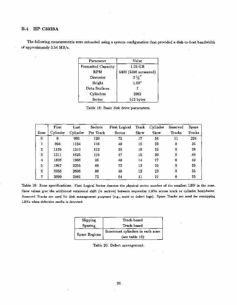
B.4 HP C3323A

The following measurements were extracted using a system configuration that provided a disk-to-host bandwidthof approximately 3.54 MB/s.

Parameter Value

Formatted Capacity 1.05 GBRPM 5400 (5396 measured)

Diameter 3%"

Height 1.00"

Data Surfaces 7Cylinders 2982

Sector 512 bytes

Table 18: Basic disk drive parameters.

First Last Sectors First Logical Track Cylinder Reserved Spare

Zone Cylinder Cylinder Per Track Sector Skew Skew Tracks Tracks

0 0 993 120 73 17 34 11 224

1 994 1134 116 48 16 33 0 352 1135 1310 112 23 16 32 0 28

3 1311 1625 104 47 15 30 0 49

4 1626 1966 96 48 14 27 0 49

5 1967 2255 88 72 13 25 0 35

6 2256 2608 80 48 12 23 0 35

7 2609 2981 72 64 11 21 0 35

Table 19: Zone specifications. First Logical Sector denotes the physical sector number of the smallest LBN in the zone.

Skew values give the additional rotational shift (in sectors) between sequential LBNs across track or cylinder boundaries.Reserved Tracks are used for disk management purposes (e.g., error or defect logs). Spare Tracks are used for remappingLBNs when defective media is detected.

Slipping Track-based

Sparing Track-based

Spare RegionsInnermost cylinders in each zone

(see table 19)

Table 20: Defect management.

36

Number of Segments 2

Writable Segments 1

Segment Size 256 KBRead-on-arrival NoWrite-on-arrival NoRequested Data Can be pushed out by prefetch

READ hits on WRITE data Allowed

PrefetchObeys Caching Mode Page parameters

Default: 64 KB

Table 21: On-board cache characteristics.

I Value IOverhead

Read Hit After Read 0.35 ms

Read Hit After Write 1.39 ms

Read Miss After Read 2.50 ms

Read Miss After Write 2.50 msWrite After Read 3.29 fiS

Write After Write 2.92 ms

Read Completion 0.24 ms

Write Completion 0.00 ms

Head Switch 0.65 ms

Write Settle 0.07 ms

Table 22: 50th percentile command processing, completion, and mechanical overheads.

37

20 5

, ,

, 415

,, ,

li)',

li)' ---,§. ,§.3Q) Q)

~ 10 ~ -Maximum~

~2 --- MeanQ)

-Maximum~ ~--- Mean5

500 1000 1500 2000 2500Seek Distance (Cylinders)

20 40 60 80Seek Distance (Cylinders)

100

(a) Full seek curve (b) Expanded view of short seeks

Figure 15: Extracted seek curves.

38