/ 2d C

BALL BEARING VIBRATIONS

AMPLITUDE MODELING AND TEST COMPARISONS

N95- 27286

,-/js-2 97/

Richard A. Hightower II1" and Dave Bailey"

ABSTRACT

Bearings generate disturbances that, when combined with structural gains of amomentum wheel, contribute to induced vibration in the wheel. The frequencies

generated by a ball bearing are defined by the bearing's geometry and defects. The

amplitudes at these frequencies are dependent upon the, actual geometry variations

from perfection; therefore, a geometrically perfect bearing will produce no amplitudes at

the kinematic frequencies that the design generates. Because perfect geometry can

only be approached, emitted vibrations do occur. The most significant vibration is at

the spin frequency and can be balanced out in the build process. Other frequencies'

amplitudes, however, cannot be balanced out.

Momentum wheels are usually the single largest source of vibrations in a spacecraft

and can contribute to pointing inaccuracies if emitted vibrations ring the structure or are

in the high-gain bandwidth of a sensitive pointing control loop. It is therefore important

to be able to provide an apriori knowledge of possible amplitudes that are singular in

source or are a result of interacting defects that do not reveal themselves in normal

frequency prediction equations.

This paper will describe the computer model that provides for the incorporation ofbearing geometry errors and then develops an estimation of actual amplitudes and

frequencies. Test results were correlated with the model.

A momentum wheel was producing an unacceptable 74 Hz amplitude. The model was

used to simulate geometry errors and proved successful in identifying a cause that wasverified when the parts were inspected.

INTRODUCTION

Vibration in spacecraft has always been of concern when considering component life

and performance issues. Of particular concern is the effect on pointing accuracies ofinstruments that must perform despite emitted vibrations from other on-board devices.

Honeywell Inc., Satellite Systems Operation, Glendale, Arizona

301

https://ntrs.nasa.gov/search.jsp?R=19950020866 2018-07-02T00:13:21+00:00Z

o m

Momentum wheels provide momentum control for space vehicles. The wheel is

supported by conventional ball bearings, which generate their own vibration due tonormal manufacturing geometry errors and/or defects. To gain a better understanding

of how these geometry errors and defects contribute to induced vibration from the

bearings, a model was developed and applied to study these motions. This model is

actually an extension of a static model developed to analyze mounted and operating

preload, ball loading, and contact stresses.

MODEL DESCRIPTION

The Motion Model was developed as an analytical tool that could be utilized to predict

bearing motion. If bearing motion could be predicted, then ultimately individual bearing

parts could be matched to yield bearing assemblies (bearing pairs in the momentum

wheel application) that produce minimal bearing motions.

The Motion Model is a quasistatic model that actually analyzes bearing motion in 512

(or less if desired) incremental steps as a static model. This number of steps wasdetermined as sufficient to yield adequate frequency resolution over the frequency

spectrum of interest (0 - 200 Hz). The data from these 512 steps is run through adiscrete Fast Fourier Transform (FFT) Routine, developed by Dave Bailey, Honeywell

Satellite Systems Operation (SSO), to yield a frequency spectrum of radial and axial

amplitudes. The FFT Routine requires 2n steps to generate a spectrum from the model

data. The number of steps selected is divided by the number of inner ring (e.g., shaft)

rotations. The number of shaft rotations input into the model represents the number of

inner ring rotations that will bring the inner ring and balls back to their original starting

position, taking into account nominal bearing geometry. For the 305 size bearing

referenced in this paper, 19 inner ring (e.g., shaft) rotations are required.

Motions generated by the model include radial (designated k & v by the model) and

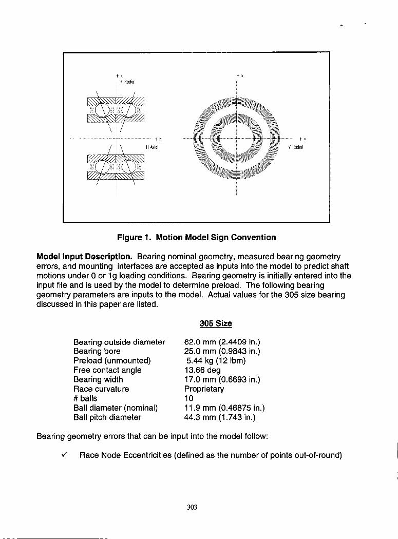
axial (designated h) forces and deflections. Figure 1 shows the sign convention used.

302

\

+k

K Radial

/

+k

+h +v

H Axial V Radial

Figure 1. Motion Model Sign Convention

Model Input Description. Bearing nominal geometry, measured bearing geometryerrors, and mounting interfaces are accepted as inputs into the model to predict shaftmotions under 0 or lg loading conditions. Bearing geometry is initially entered into theinput file and is used by the model to determine preload. The following bearinggeometry parameters are inputs to the model. Actual values for the 305 size bearingdiscussed in this paper are listed.

305 Size

Bearing outside diameterBearing borePreload (unmounted)Free contact angleBearing widthRace curvature# balls

Ball diameter (nominal)Ball pitch diameter

62.0 mm (2.4409 in.)

25.0 mm (0.9843 in.)5.44 kg (12 Ibm)13.66 deg17.0 mm (0.6693 in.)Proprietary10

11.9 mm (0.46875 in.)44.3 mm (1.743 in.)

Bearing geometry errors that can be input into the model follow:

v" Race Node Eccentricities (defined as the number of points out-of-round)

303

Input Options - 1, 2, 3, or 4 Node- Node 1 is a simple eccentricity, i.e., the bore axis offset from the

race axis

- Node 2 is a 2 point out-of-round, i.e., oval shaped

- Node 3 is a 3 point out-of-round

- Node 4 is a 4 point out-of-round

Eccentricity-Inner

-Inner

values can be input for:

and/or outer radial eccentricity

and/or outer axial eccentricity

Race Talyrond Data (radial only)- Digitized data. A sample plot of a typical error data file is shown in

Figure 2.

TALYROND DATA

ERROR FILE7

6

5

2

i'0 ,

I .'12 330 360

-3

-4

-5

-6

-7

,/

,/

Figure 2. Talyrond Error Plot

Contact Angle difference (row 1 versus row 2)

Ball Geometry ErrorsSize Errors generally input as a random ball size deviation

Specific ball size deviations can also be entered

Spacing Errors input for biased cage applications

3o4

Program-generated geometry errors from previous error inputs, together with themeasured Talyrond errors, are summed and input into the main model for the motionanalysis.

In addition to the above inputs, the model will also allow the inner and/or outer rings tobe "clocked" relative to each other. This clocking allows the model to analyze motionsfor various face-to-face alignments of the bearing rings. In addition, the effect ofphasing the inner or outer ring radial eccentricities relative to the axial eccentricities atspecified angles can be investigated.

Figure 3 is a sample input file 1 used by the Motion Model.

Motion plots are generated by the model and are shown as the number of steps versusdeflection amplitude. Information that can be extracted from these plots includes notonly deflection ranges but motion phase information amongst the three components.Figure 4 is an example of a motion plot.

In addition to motion plots, frequency spectrum plots versus radial and axial amplitudescan also be generated. Figure 5 is an example of a frequency plot.

Other plots that can be generated include force (N) and acceleration (g's) versusfrequency.

MODEL VALIDATION

Validation of the Motion Model was an important first step towards gaining anunderstanding of how the model worked and determining what key bearing parametersneeded to be included in the model. A program verification test matrix was thereforedeveloped to review motion and FFT plots generated by the model and to ensure thatthe test cases agreed with expected results.

Analytical Test Matrix. The intent of the test matrix was to look at each bearinggeometry error independently and combined, to review the motion and FFT output ofeach test case, and to determine if the output was as expected.

The analytical test matrix included:Perfect part geometriesRadial and axial eccentricities for 1 node to 4 node geometry errorsBall size errors

Ball spacing errorsTwo balls missingShaft unbalance forces

0g (space environment) and lg (ground environment) loading

1 Inputs shown not specific to this paper.

305

?PROBLEM SET DESCRIPTION .....................................................

61071gF3 - VER 5.2 JULY 5,1991 RUN DATE 08/09/91

?DESCRIPTION ..................................................................

IG GRAVITY CASE - BIASED CAGE - OUTER CLOCKED 90

?NO ROWS I?DF/DT/DB

-2. -I.

?STRADDLEI?PRELOAD

.6693 12.0

?FMUS I?FMUL

.07 .07

?SH TURNSI?SHAFT WT

19.

? ROW NO I?#-BALLS

i. i0.0

?IR PRESS ?IR HD/D

.000200 .26

?OR PRESS ?OR HD/D

-.00037 .26

?E-SHAFT I?E-BRG

32.E6 32.E6

?TC-SHAFTI?TC-BRG

7.0E-6 7.5E-6

?THRUST

0.0

?CASE

i.

?FMUC

.07

?UNBAL

0.

?BALL DIA

.46875

?IR-DAM/D

.26

?OR-DAM/D

.26

?E-HSG

32 .E6

?TC-HSG

6.2E-6

?RADIAL

20.

?FMU-PRLD

.15

?L-VIS CS

140.

?UNBA ANG

0.

?FREE CA

13.66

?IR-WIDTH

.6693

?OR-WIDTH

.6693

?PR-SHAFT

.32

?OT-SHAFT

80.

?APHA/MOM

?RATE

?L-QUAN

.13

?ITER_TOL

.025

? E

1.743

?SHAFT ID

? BRG OD

2.4409

?PR-BRG

.32

?OT-IR

80.

.......... ROW 1 GEOMETRY ERRORS (MICROINCHES)

I?IR RAD I?OR RAD ?IR AXIAL ?OR AXIAL?NODE

i. 30.0 40.0 -30.0 30.0

2.

3.

4.

?SHIFT IRI?SHIFT OR 1 l

90.

? NSIR I? NSOR I?BSIZE I?

12.o 1.o o.ooooo5.............. BALL SPACEING ERRORS

INNER EVERY 30 deg

? RPM ? STEPS

2000. 512.

?GAP ?FLUSH

-.000005

?CLEAR ?XRUN

.010

?DIFF_CA ?VRADIAL

-.140

? FI ? FO

.54 .55

?BRG BORE ?IR-CLAMP

.9843 i00.

? HSG OD ?OR-CLAMP

5. i00.

?PR-HSG IDENSITY

.30 .150

?OT-OR ]?OT-HSG

70. 75.

--- RADIAL TO AXIAL DEG

?PHASE IRiPRASE OR

?CONTROL

i.

?FILM

?NUSE

?TEST

? BGAP

?IRC-FMU

.I

?ORC-FMU

.i

? DELR

? DELH

IR RADIAL

?SHIFT

I?IR FILE I?ORFILE IIR721FX.RND OR520FX.RND

i? i? l

(degrees) ......................

?BALL1 [?BALL2 I?BALL3 I?BALL4 I?BALL5 I?BALL6 I?BALL7 I?BALL8 I?BALL9 I?BALLI01

?BA_L___?BALL_2_?BALL_3_?BALL_4_?BALL_5_?BAL__6_?BAL__7_?BA___8_?BALL_9_?BA_L2__

.............. BALL DIAMETER ERRORS (micro-inches) ................

?BALL1 I?BALL2 1?BALL3 I?BALL4 I?BALL5 I?BALL6 I?BALL7 I?BALL8 I? BALL9 I ?BALL10

?BALLIII?BALLI21?BALLIBI?BALLI41?BALLI5I?BALLI61?BALLI71?BALLI81?BALLI91?BALL20

.......... ROW 2 GEOMETRY ERRORS (MICROINCHES) RADIAL TO AXIAL DEG IR RADIAL

?NODE I?IR RAD I?OR RAD I?IR AXIALI?OR AXIAL ?PHASE IRIPHASE OR ?SHIFT

i. 20.0 45.0 30.0

2.

3.

4.

?SHIFT IRI?SHIFT omJ I

? NSIR I? NSOR I?BSIZE I?1.0 1.0 0.000005

.............. BALL SPACEING ERRORS

-30.0

I?IR FILE I?ORFILE IIR672FX.ENDOR353FX.RND

I? I? I

(degrees) ......................

?BALL1 I?BALL2 I?BALL3 I?BALL4 I?BALL5 I?BALL6 I?BALL7 I?BALL8 I?BALL9 I?BALLI0

?BALLIII?BALLI21?BALLI31?BALLI41?BALLI51?BALLI61?BALLI71?BALLI81?BALLI91?BALL20

.............. BALL DIAMETER ERRORS (micro-inches) ................

?BALL1 I?BALL2 I?BALL3 1?BALL4 I?BALL5 I?BALL6 I?BALL7 I?BALL8 I?BALL9 [?BALL10

?BALLIII?BALLI21?BALLI31?BALLI41?BALLI51?BALLI61?BALLI71?BALLI81?BALLI9I?BALL20

Figure 3. Model Input File

306

=,

H, K, & V MOTIONS vs STEPS

3

2

I

0

-2

-3

0

• \,

Z : , l

I I I I I I I I

20 40 60 80 100 120 140 160 180

IR ROTATION STEP

_H ..... K ....... V I

Figure 4. Motion Plot

uJa

.Ja.5,<

100

10

1

0.1

0.01

H, K, & V FFT'S vs FREQUENCY

x

I I I I I

20 40 60 80 100 120 140 160 180 200

FREQUENCY

I--.--H --o--K --x--VI

Figure 5. Frequency Plot

A total of 122 test cases were run and reviewed.

Several iterations of these test cases were completed because each iteration revealedadditional model errors and identified model enhancements. Finally, all 122 test caseresults were considered acceptable and it was concluded that the model was valid.

307

Figures 6 and 7 are shown to illustrate the sensitivity of the model to inputted geometry

errors. Figure 6 shows a frequency plot for a 0.10 gm (4 gin.) cosine ball size

distribution error input; no other geometry errors were input. As expected, the model

generated a disturbance at the ball group frequency, a 37 Hz peak of 0.10 gm (4 gin.)amplitude.

Figure 7 is an output plot for the same cosine ball size distribution and a 0.09 kg

(0.2 Ibm) shaft unbalance force applied. Note the motion response at the 100 Hz spin

frequency.

u.Ia

..I

COSINE BALL DISTRIBUTION

I0

0.1

0.01 X-XXX.X_(X0.0o1 0.0001 _[ --_''_._ {_...ui _l_r._ ._ _,_

0 20 40 60 80 100 120 140 160 180 200

FREQUENCY, (Hz)

I--=--H --=--K --X--V I

Figure 6. Cosine Ball Distribution

uJ¢3

..J

.=

10

1

0.1

0.01

0.001

0.0001

.09kg (.2 Ibm) SHAFT UNBALANCE

x

0 20 40 60 80 100 120 140 160 180 200

FREQUENCY (Hz)

[--=-- H --D-- K --X--V I

Figure 7. Shaft Unbalance

BEARING DISTURBANCES

Two frequencies have been identified as being of particular interest in the investigation

of bearing disturbance effects on momentum wheels. These frequencies are 74 and

100 Hz. A momentum wheel was producing an unacceptable 74 Hz axial disturbance.The model was used to simulate geometry errors and identify a cause.

308

Frequency Drivers. The model was run using actual measured data from a 305 size

bearing pair to investigate effects on bearing motion due to inner and outer ring clocking

and phasing. This data included measured contact angle, face stickout, and borediameter. In addition, axial runout and unmounted preload was input to the model for

the bearing pair. Inspection data for each bearing ring (inner and outer) includedrace/bore radial runout and race radial roundness. Talyrond plots of the individual rings

were digitized and converted to error files for the model. A + 0.13 lim (+ 5 llin.) randomball size error distribution was input into the model, which is the size variation specified

for Anti-Friction Bearing Manufacturers Association (AFBMA) Grade 3 balls. Also, ball

position errors were included to account for biased cage geometry effects.

Cases were run for 0g and lg loading.

Table 1 lists the cases that were run in the model, the parameters that were varied, and

the effect on the Model output.

Table 1. Actual Bearing Results

Case

l(0g)

2 (lg)

3 (0g)

4 (0g)

5(lg)

6 (0g)

7(lg)

8 (0g)9(lg)

Parameter Varied

Inner rings clocked every 30 °

Same as above +

Same size balls

Inner rings clocked every 30 ° for every 30 °

clocking of outer ring

Phase radial to axial inner ring ecc. 90 ° for

every 90 ° phasing of radial to axial outer ringecc. (row 1 only)

Shift row 1 rings +2.54 _m (+100 pin), row 2

rings -2.54 l_m (-100 l_in)

Model Results

Negligible change inamplitudes at all

frequencies

Negligible change in

amplitudes

Negligible change in

amplitudes

Negligible change inamplitudes

Large increase in axialamplitudes at 74 and

100 Hz

Results from these runs follow:

Inner ring clocking has no effect on amplitudes

Outer ring clocking has no effect on amplitudes

Random ball size change has a small effect on amplitudes at 37 Hz

Phasing of eccentricities has a minimal effect on amplitudes at 100 Hz

Loading (0g versus lg) has an effect on 100 Hz axial and 74 Hz radial

components

3o9

In completing the model verification test runs, bearing disturbance frequencies,geometry error input, and the component drive (radial or axial), relationships werenoted. Table 2 summarizes the relationship of these factors.

Table 2. Bearing Disturbances

Frequency Disturbance Causes Component

74 Hz

100 Hz

Ball size (random)

Ball position (biased cage)

Outer ring geometry combined with ball size variation

Outer ring geometry combined with ball size and ballposition

1 large/9 small balls

Inner race axial eccentricity (node 1)

Inner race radial eccentricity (node 1)

Rotor unbalance force

Radial/Axial

Radial

Radial

Radial/Axial

Radial

Radial/Axial

Radial/Axial

Radial

From Table 2 it is evident that 74 Hz axial motion is controlled by ball group symmetryand/or outer race geometry.

Momentum Wheel Amplitude Prediction. The most likely cause of the 74 Hz axialbearing motion generated in the momentum wheel is outer ring geometry errors. Onescenario that could cause this geometry error is the bearing cartridge "squeezing" thebearing outer ring. This squeezing is actually a two-point interference fit between thebearing cartridge and the bearing outer ring. It was theorized that the cartridge hadpossibly become egg-shaped (i.e., node 2 error) as a result of slots that were cut intothe cartridge to accommodate other hardware. These slots could have stress-relievedthe part, allowing the cartridge to deform and squeeze the outer rings of the bearings.

The outer ring squeeze was modeled as a 2 node radial geometry error in row 1 and row2 of the bearing outer rings. Figure 8 shows the node 2 error relative to a "perfect" ring.

310

Figure 8. Outer Ring Node 2 Error

Bearing inspection data for the bearings mounted in the momentum wheel was used forgeometry error inputs. These inputs, in addition to mounting and loading parameters, areas follows:

• Ball position error biased cage

• Random ball size +0.13 pm _ 5 pin.)

• Node 1 eccentricity

Row 1

Row 2

Talyrond dataBore/Shaft interference

Bearing OD clearancelg loading

0.76 pm (30 pin.) inner radial

1.02 pm (40 pin.) outer radial0.76 pm (30 pin.) inner axial

0.76 pm (30 pin.) outer axial

0.51 pm (20 pin.) inner radial1.14 pm (45 pin.) outer radial

0.76 pm (30 pin.) inner axial

0.76 pm (30 pin.) outer axialdigitized data

2.54 pm (100 pin.)

9.40 pm (370 pin.)

Several cases were modeled to compare the axial amplitudes for different node 2 errorvalues. Cases were run with equal node 2 errors in both rows, 2x error in row 1 versus

row 2, 3.81 pm (150 pin.) error difference in row 1 versus row 2, and 7.62 pm (300 pin.)error in row 1 versus row 2. These inputs are summarized in Table 3.

311

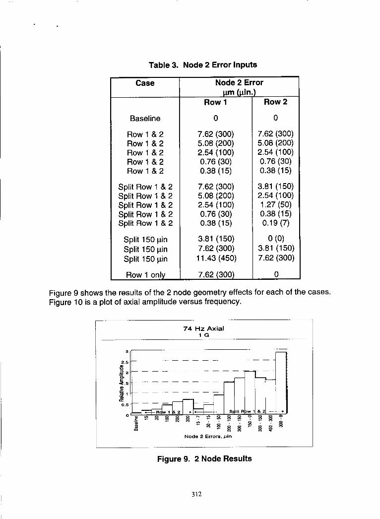
Table 3. Node 2 Error Inputs

Case

Baseline

Row 1 & 2Row 1 & 2Row 1 & 2Row 1 & 2Row 1 & 2

Split Row 1 & 2Split Row 1 & 2Split Row 1 & 2Split Row 1 & 2Split Row 1 & 2

Split 150 ginSplit 150 gin

Split 150 gin

Row 1 only

Node 2 Error

gm (ldn.)Row I

0

7.62 (300)5.08 (200)2.54 (100)0.76 (30)0.38 (15)

7.62 (300)5.08 (200)2.54 (100)0.76 (30)0.38 (15)

3.81 (150)

7.62 (300)

11.43 (450)

7.62 (300)

Row 2

0

7.62 (300)5.08 (200)2.54 (100)0.76 (30)0.38 (15)

3.81 (150)2.54 (100)1.27 (50)0.38 (15)0.19 (7)

o(o)3.81 (15o)7.62 (300)

0

Figure 9 shows the results of the 2 node geometry effects for each of the cases.

Figure 10 is a plot of axial amplitude versus frequency.

3

.-_=2

0.5

O

74 Hz Axial1G

Node 2 Errors, pin

Figure 9. 2 Node Results

312

AXIAL MOTION

1

0.1 -

0.00_

o 32 64 96 128 160 192 224 256 288 320

FREQUENCY (Hz)

[--=--m_SEUNE--_--150_0--*--3o0_oI

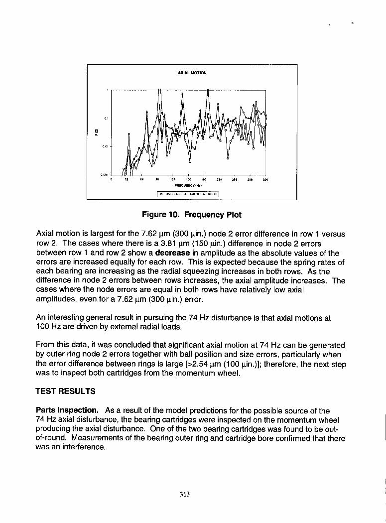
Figure 10. Frequency Plot

Axial motion is largest for the 7.62 llm (300 _in.) node 2 error difference in row 1 versusrow 2. The cases where there is a 3.81 lim (150 _in.) difference in node 2 errors

between row 1 and row 2 show a decrease in amplitude as the absolute values of theerrors are increased equally for each row. This is expected because the spring rates ofeach bearing are increasing as the radial squeezing increases in both rows. As thedifference in node 2 errors between rows increases, the axial amplitude increases. Thecases where the node errors are equal in both rows have relatively low axialamplitudes, even for a 7.62 lim (300 _in.) error.

An interesting general result in pursuing the 74 Hz disturbance is that axial motions at100 Hz are driven by external radial loads.

From this data, it was concluded that significant axial motion at 74 Hz can be generatedby outer ring node 2 errors together with ball position and size errors, particularly whenthe error difference between rings is large [>2.54 lim (100 liin.)]; therefore, the next stepwas to inspect both cartridges from the momentum wheel.

TEST RESULTS

Parts Inspection. As a result of the model predictions for the possible source of the74 Hz axial disturbance, the bearing cartridges were inspected on the momentum wheelproducing the axial disturbance. One of the two bearing cartridges was found to be out-of-round. Measurements of the bearing outer ring and cartridge bore confirmed that therewas an interference.

313

Wheel Test Results. A series of tests were conducted to verify that the out-of-round

cartridge was indeed the driver. Frequency data was taken with the 305 bearing pair

installed in the out-of-round cartridge and again with the bearings installed in a roundcartridge. The test was repeated with the bearings installed in the out-of-round cartridge

to check repeatability of the measurements. Frequency output data for the out-of-round

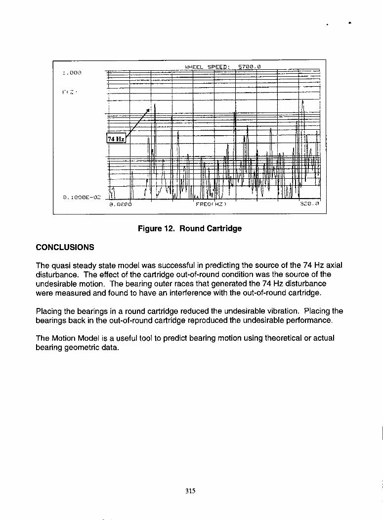
cartridge is shown in Figure 11, while Figure 12 illustrates frequency data for the round

cartridge. Note the significant decrease in amplitude at 74 Hz for the round cartridge.

These tests confirmed that the out-of-round cartridge did cause the outer ring to distort,generating the 74 Hz axial motion and producing over 3x the disturbance at 74 Hz than

bearings installed in the round cartridge.

1.000

F_I7" J

O.I@OOE-@2

I ! ::

I

i

]1 i

: ZIA/

0.0_00

Figure 11. Out-of-round Cartridge

314

D

I_IHEEL SPEED: 57_.0

t

B.B_B , PEQ(H-I 32@._

Figure 12. Round Ca_ridge

I. EI';3E1

F f. Z )

EI.I@GOE-02

CONCLUSIONS

The quasi steady state model was successful in predicting the source of the 74 Hz axialdisturbance. The effect of the cartridge out-of-round condition was the source of the

undesirable motion. The bearing outer races that generated the 74 Hz disturbancewere measured and found to have an interference with the out-of-round cartridge.

Placing the bearings in a round cartridge reduced the undesirable vibration. Placing the

bearings back in the out-of-round cartridge reproduced the undesirable performance.

The Motion Model is a useful tool to predict bearing motion using theoretical or actual

bearing geometric data.

315