NAL-Pub-73/86-THY

Nuclear Charge Exchange Corrections to Lieptonic Pion

Production in the (3, 3)-Resonance Region

Stephen L.. Adler

Institute for Advanced Study, Princeton, New Jersey 08540

and

National Accelerator L.aboratory,* Batavia, Illinois 60510

and

Shmuei Nussinov t and E. A. Paschos

National Accelerator Laboratory, Batavia, Illinois 60510

ABSTRACT

We discuss nuclear charge exchange corrections to leptonic pion

production in the region of the (3,3) resonance, both from a phenomenol-

ogical viewpoint and from the evaluation of a detailed model for pion

multiple scattering in the target nucLeus. Using our analysis, we estimate

the nuclear corrections needed to extract the ratio

R = [F(v~ t n--vF+ntiO) t u (VpSp’v P

tp*OJj /2F (v~+ll”)l- tp+aO)

from neutral current search experiments using 13Al 27

and other nuclei

as targets.

::Operated-by Universities Research Association, Inc., under contract with the U. S. Atomic Energy Commission.

tPermanent Address: Tel-Aviv University, Ramat-Aviv, Tel-Aviv, Israel.

-2-

1. INTRODUCTION

Although weak interaction experiments on hydrogen and deuterium

targets are most readily interpreted theoretically, experimental consider-

ations necessitate the use of complex nuclear targets in many of the cur-

rent generation of accelerator neutrino experiments. As a result, in such

experiments, corrections for nuclear effects must be made in order to ex-

tract free nucleon cross sections from the experimental data. Our aim in

the present paper is to analyze these corrections’in a particularly simple

case: that of leptonic single pion production in the region of the (3, 3) reson-

ance. This reaction has gained prominence recently because measurement

of the ratio

u(V +n-cV tntr’) tcr(v tp - v t p t VO) R= k

2u (VP-+ n - p-t p t Tr”) 0)

appears to be one of the better ways of searching for hadronic weak neu-

tral currents. 1

Experiments measuring R use aluminum (and in some

cases ‘also carbon) as target materials, so the experimentally measured

quantity is actually (T I , T” denote unobserved final target states)

U(Y tT--v +T’tT’) R’ (T) =

- p-t T”t no) 9 T=

2u(vpt T 13A127, 6c12* (2)

As Perkins has emphasized, 2 nuclear charge exchange effects can cause

substantial differences between R and RI, which makes reliable es-

timation of these effects an important ingredient in correctly interpreting

the experiments. Fortunately, pion production in the (3, 3) region is

also a particularly favorable case for theoretical analysis, primarily

-3-

because the elasticity of the (3, 3) resonance implies that nuclear effects

will not bring multipion or other more complex hadronic channels into

Play l

Our discussion is organized as follows. In Section 2 we introduce

our basic phenomenological assumption, that leptonic pion production on

a nuclear target may be represented as a two-step compound process, in

which pions are first produced from constituent nucleons with the free

lepton-nucleon cross section (apart from a Pauli principle reduction fact-

or), and subsequently undergo a nuclear interaction independent of the i-

dentity of the leptons involved in the production step. This assumption al-

lows us to isolate nuclear effects (pion charge exchange and absorption)

ina3x3 “charge exchange matrix.” We analyze the structure of the

charge exchange matrix in the particularly simple case of an isotopically

neutral target nucleus. [ For 13A1 27

, with a neutron excess of 1 and a

corresponding isospin of l/2, the approximation of isotopic neutrality

should be quite adequate. For 12

fF ’ of course, no approximation is in-

volved. ] Our mtiih.phenomenological result is that parameters of the

charge exchange matrix, which can be measured in high rate pion electro-

production experiments, can be used to calculate the nuclear corrections

to the weak pion production process, and in particular to give the con-

nection between R’ and R. In Section 3 we develop a detailed multiple

scattering model. for the charge exchange matrix. Our model is quite

similar to a successful calculation by Sternheim and Silbar3 of pion

production in the (3,3) resonance region induced by protons incident on

-4-

nuclear targets, and uses the nuclear pion absorption cross section which

they determine (as well as the experimental pion-nucleon charge exchange

cross section) as inputs. The principal difference between our calculation

and that of Sternheim and Silbar (apart from obvious changes stemming

from the fact that they deal with a strongly absorbed, rather than a weakly

interacting projectile) is that we use an improved approximation to the

multiple scattering problem, based on a one-dimensional scattering solu-

tion introduced by Fermi in the early days of neutron physics. 4

Using our

model for the charge exchange matrix, and a theoretical calculation of free

nucleon electro- and weak-pion production which has been described else-

where, 5

we present detailed predictions for R’ in the Weinberg weak inter-

action theory and some of its variants. We also use the production model to

test averaging approximations implicit in the phenomenological discussion

of Section 2. In Section 4 we summarize briefly our conclusions. Three

appendices are devoted to mathematical details. In Appendix A we formu-

late and solve the one-dimensional scattering problem which forms the basis

for the approximate solution of the three-dimensional multiple scattering

problem actually encountered in our model. To calibrate this approjrima-

tion, in Appendix B we compare the approximate solution with the exact

multiple scattering solution for the simple case of isotropic scattering

centers uniformly distributed within a sphere. Finally, in Appendix C we

collect miscellaneous formulas for cross sections and for Pauli exclusion

factors which are needed in the text.

-5-

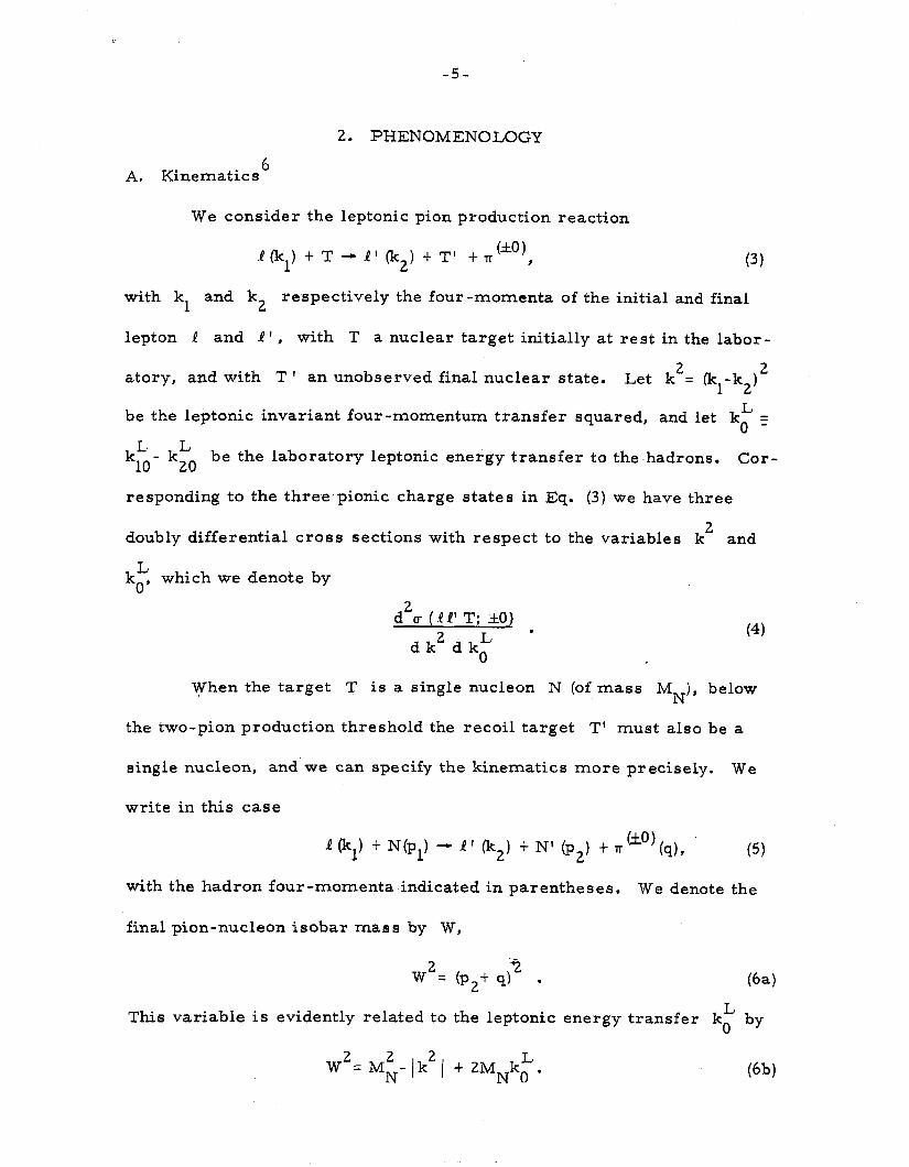
2. PHENOMENOLOGY

A. Kinematics 6

We consider the leptonic

I(k)+TdP’(k 1 2

pion production reaction

) t T’ + r(&‘), (3)

with kl and k2 respectively the four-momenta of the initial and final

lepton 1 and I’, with T a nuclear target initially at rest in the labor-

atory, and with T ’ an unobserved final nuclear state. Let k2= (‘kl-k2)2

be the leptonic invariant four-momentum transfer squared, and let

kL’- kL 10 20

be the laboratory leptonic energy transfer to the hadrons. Cor-

responding to the three,pionic charge states in Eq. (3) we have three

doubly differential cross sections with respect to the variables k2 and

kt, which we denote by

d2a (I!’ T; ItO)

d k2 d ko” . (4)

When the target T is a single nucleon N (of mass MN), below

the two-pion production threshold the recoil target T’ must also be a

single nucleon, and we can specify the kinematics more precisely. We

write in this case

1 $1 + Np 1 1 - 1’ (k 2 1 + N’ (P,) + r k”)(q),

with the hadron four-momenta indicated in parentheses. We denote the

final pion-nucleon isobar mass by W,

- w2= (p2t q)z .

L This variable is evidently related to the leptonic energy transfer k. by

W2= M;- (k2 ( -t 2MNk;. W

i’ I

-6-

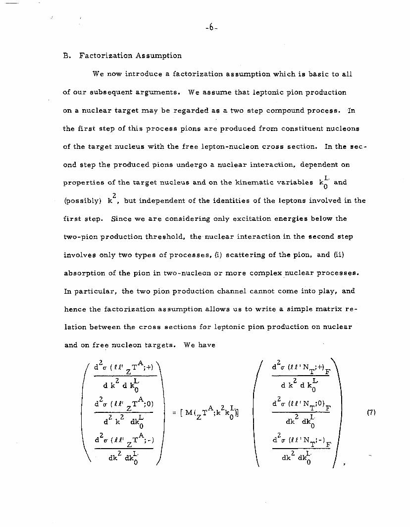
B. Factorization Assumption

We now introduce a factorization assumption which is basic to all

of our subsequent arguments. We assume that leptonic pion production

on a nuclear target may be regarded as a two step compound process. In

the first step of this process pions are produced from constituent nucleons

of the target nucleus with the free lepton-nucleon cross section. In the sec-

ond step the produced pions undergo a nuclear interaction, dependent on

properties of the target nucleus and on the kinematic variables kt and

(possibly) k2, but independent of the identities of the leptons involved in the

first step. Since we are considering only excitation energies below the

two-pion production threshold, the nuclear interaction in the second step

involves only two types of processes, (i) scattering of the pion, and (ii)

absorption of the pion in two-nucleon or more complex nuclear processes.

In particular, the two pion production channel cannot come into play, and

hence the factorization assumption allows us to write a simple matrix re-

lation between the cross sections for leptonic pion production on nuclear

and on free nucleon targets. We have

= [ M(,TA;k2k;)]

d k2 d kt

d’o- (11’ NT;O$

dk2 dk;

d2a (41’ NT;+,

dk2 dk; i

(7)

-7-

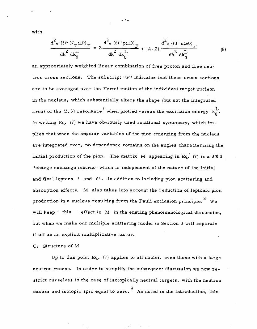
with

d 2

(r (11’ NT;kO)F = Z d2a (ml’ p;kO) F d2a (11 t n;&O) F

dk2 dk; dk2 dk; t (A-Z)

dk2 dk;

an appropriately weighted linear combination of free proton and free neu-

(8)

tron cross sections. The subscript “Ff’ indicates that these cross sections

are to be averaged over the Fermi motion of the individual target nucleon

in the nucleus, which substantially alters the shape (but not the integrated

area) of the (3, 3) resonance 7

when plotted versus the excitation energy k L 0’

In writing Eq. (7) we have obviously used rotational symmetry, which im-

plies that when the angular variables of the pion emerging from the nucleus

are integrated over, no dependence remains on the angles characterizing the

initial production of the pion. The matrix M appearing in Eq. (7) is a 3 x 3

“charge exchange matrix” which is independent of the nature of the initial

and final leptons I and 1’ D In addition to including pion scattering and

absorption effects, M also takes into account the reduction of leptonic pion

production in a nucleus resulting from the Pauii exclusion principle. 8 We

will keep ‘.. this effect in M in the ensuing phenomenological discussion,

but when we make our multiple scattering model in Section 3 will separate

it off as an explicit multiplicative factor.

c. Structure of M

Up to this point Eq. (7) applies to all nuclei, even those with a large

neutron excess. In order to simplify the.subsequent discussion we now re-

strict ourselves to the case of isotopically neutral targets, with the neutron

excess and isotopic spin equal to zero. 9

As noted in the Introduction, this

-8-

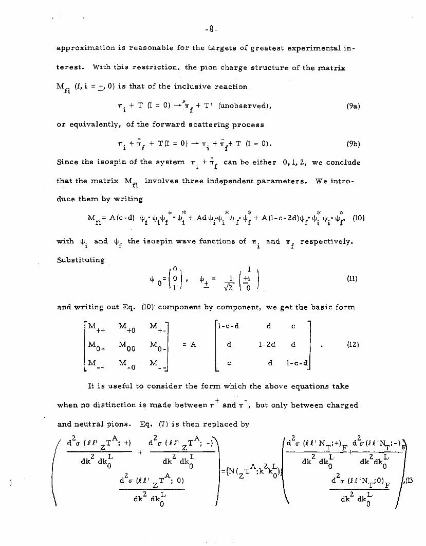
approximation is reasonable for the targets of greatest experimental in-

terest. With this restriction, the pion charge structure of the matrix

Mfi (f, i = 2, 0) is that of the inclusive reaction

‘rri t T (I = 0) -Titf t T’ (unobserved), (94

or equivalently, of the forward scattering process

ri t if t T(I = 0) - TT. t ;,t T (I = 0). 1

(9b)

Since the isospin of the system IT. t Gf 1 can be either 0, 1,2, we conclude

that the matrix Mfi involves three independent parameters. We intro-

duce them by writing

9: Mfi= A(c-d) Gf’ tj~$, l L/J; t Ad t$&“t$ f* $;” t A(l-c-2d)Gf* Jlf ~$0 $;, (10)

with 4: and $, the isospin wave functions of TT i

and IT f respectively.

1 0

4J o= 0 1

1 I

Substituting

and writing out Eq. (10). component by component9 we get the basic form

(1)

It is useful to consider the form which the above equations take

when no distinction is made between r t

and TT-, but only between charged

and neutral pions. and neutral pions. Eq. (7) is then replaced by Eq. (7) is then replaced by

d’cr (11’ ZTA: t) d’cr (11’ ZTA: t)

dk2 dk; t

dk2 dk: d2F;;+$‘05?

d2a (11’ -TA; 0) L

dk2 dk;

=[N(,TA;k2k;)

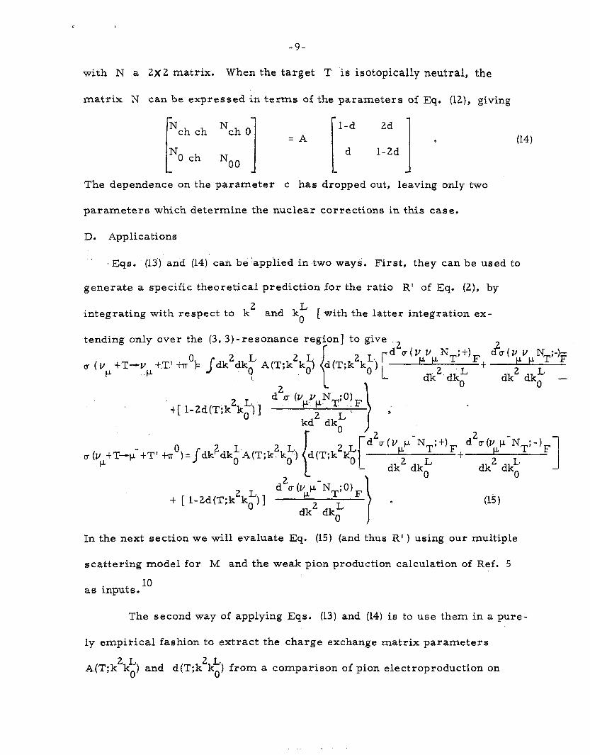
-9-

with N a 2x2 matrix. When the target T is isotopically

matrix N can be expressed in terms of the parameters of

neutral, the

Eq. (12), giving

0 (14)

The dependence on the parameter c has dropped out, leaving only two

parameters which determine the nuclear corrections in this case.

D. Applications

1 Zqs. (13’) and (14) can be ‘appiied in two ways. First, they can be used to

generate a specific theoretical prediction for the ratio R’ of Eq. (2), by

integrating with respect to k2 and kt [ with the latter integration ex-

tending only over the (3, 3)-resonance region] to give ,

c ( y tT--vll S.T.’ t,r”b fdk’dk? A(T;k2k_Lj ’ P

d2,(v v pp

J y ‘- ,U’ .-

2 1 “l

t-1 1-Zd(Tik’k,L.)] d a (yp&.$VF

,’ T L *

ST’ +a’)=

2 rWpp-NT;+)F

dk2 dk; t

t [ l-2d(T;k‘k;)]

In the next section we will evaluate Eq. (15) (and thus RI ) using our multiple

scattering model for M and the weak pion production calculation of Ref. 5

as inputs. 10

The second way of applying Eqs. (13) and (14) is to use them in a pure-

ly empirical fashion to extract the charge exchange matrix parameters

A(T;k’kt) and d(T;k’kk) from a comparison of pion electroproduction on

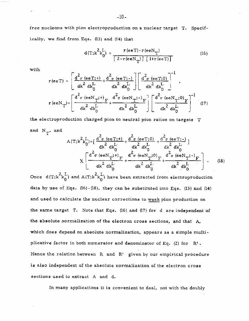
-lO-

free nucleons with pion electroproduction on a nuclear target T. Specif-

ically, we find from Eqs. (13) and (14) that

d (T;k’k;) = r (eeT)-r (eeNT)

[ 2-r(eeNT)] [ ltr(eeT)]

with i-2

d u (eeT;t) + d F (eeT;-) T f d2r (eeT*O) ID1 2

r(eeT) = 1, 1. dk2 dk;

I I ’ I dk2 dk; 1 L dk2 dk; A,

F

(16)

r(eeN d2u (eeNT;-lF1 fd2u (eeNT;O)Fle’

dk2 dk; I I

dk2 dkL J (17)

_I!- 0 J

the electroproduction charged pion to neutral pion ratios on targets T

and N T’

and

A(T;k’k;)=[ d20 (eeT; t)

dk2 dkL

t d2r (eeT;O) + d2r (eeT;-)

dk2 dk; dk2 dk; 1

)( [d”cr (eeNT;i)F d2c (eeNT;O)F d2c (eeNT;-)F -1

I dk2 dk; t

dk2 dk; t I *

dk2 .dkg. j (18 1

Once d(T;k2k:) and A(T;k’kk) have been extracted from electroproduction

data by use of Eqs. (16) - (18), they can be substituted into Eqs, (13) and (14)

and used to calculate the nuclear corrections to weak pion production on

the same target T. Note that Eqs. (16) and (17) for d are independent of

the absolute normalization of the electron cross sections, and that A,

which does depend on absolute normalization, appears as a simple multi-

plicative factor in both numerator and denominator of Eq. (2) for R1 .

Hence the relation between R and RI given by our empirical procedure

is also independent of the absolute normalization of the electron cross

sections used to extract A and d.

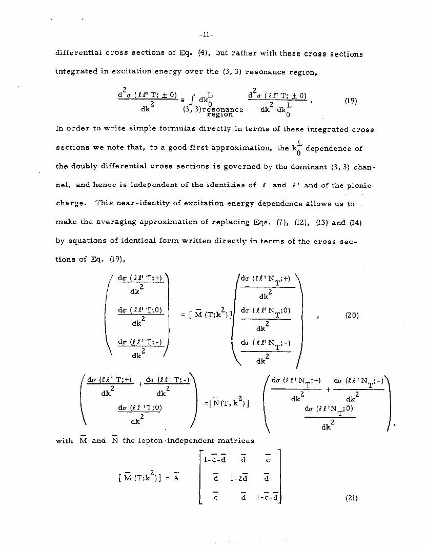
In many applications it is convenient to deal, not with the doubly

-ll-

differential cross sections of Eq. (4), but rather with these cross sections

integrated in excitation energy over the (3, 3) resonance region,

d2a (11’ T; + 0) s s dk; d2a ( em’ T; + 0)

dk2 dk2 dk; s (19)

(3,3)resonance region

In order to write simple formulas directly in terms of these integrated cross

sections we note that, to a good first approximation, the kL dependence of 0

the doubly differential cross sections is governed by the dominant (3,3) chan-

nel, and hence is independent of the identities of I and 1’ and of the pionic

charge. This near-identity of excitation energy dependence allows us to

make the averaging approximation of replacing Eqs. (7), (12), (13) and (14)

by equations of identical form written directly in terms of the cross sec-

tions of Eq. (19),

i

du (BP T;t)

dk2

du (PI’ T;O)

dk2

du (11’ T;-)

dk2 ’

with G and % the lepton-independent matrices

= [ ii (T;k’)

du (PI’ NT;+) y

dk2

du (11’ NT;O)

dk2

du (WN,;-)

dk2 I

du (11 ‘T;O) =[&(T, k’)]

[ ii (T;k’)] = x

, (20)

da (11’ NT;+) t

du (MN+-)

dk2 dk2 \

C

a

-- .-c-d

du (LP’NT;O)

dk2

w

i

I

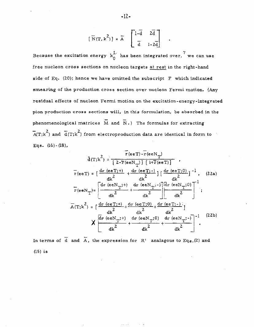
[ %(T, k2) ] = x

Because the excitation energy ki has been integrated over, 7

we can use

free nucleon cross sections on nucleon targets at rest in the right-hand

side of Eq. (20); hence we have omitted the subscript F which indicated

smearing of the production cross section over nucleon Fermi motion. (Any

residual effects of nucleon Fermi motion on the excitation-energy-integrated

pion production cross sections will, in this formulation, be absorbed in the

phenomenological matrices 6 and N. ) The formulas for extracting

A(T;k2) - 2 and d(T;k ) from electroproduction data are identical in form to

Eqs. (16) - (18),

r(eeT) -y(eeNT)

“T’k2) =’ [ 2-Y(eeNT)] [ l+F(eeT)] ’

r(eeT) = [ du (eeT;t)

2 + dr (eeZT;-) ] [ dcr (ee;:O) ] -1 , (22a)

r(eeN )- ~?~NT:t) t

dr?eN,;-)Tpu EN ;O)l-’

II T T - I- dk2 dk2 AL dk2

1 : _(

x(T;k’) = [ dr (eeT;t) +dm (eeT;O) $&r (eeT;-) ;

2 2 2 1

x /& (ztNT:t) drdieNT:O) c?(eeNT:-i)-’ (22b)

I ’ I dk2 )- dk2 ’ dk2 _I

In terms of a and A, the expression for R’ analagous to l3qs.G) and

(15) is

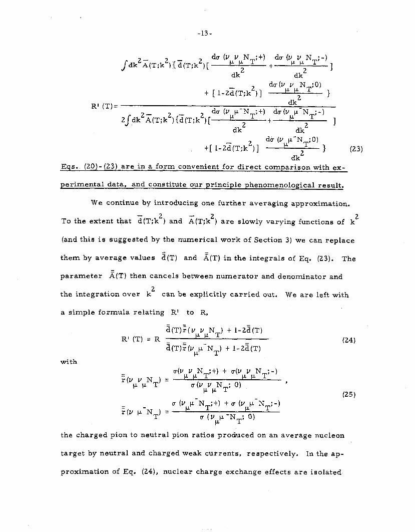
-13-

j-dk2~(T;k2)<;i(T;k2)[ du (VPYPNT; t)

t du (ZJ vP NT; -)

dk2 dk2 1

t [ l-2d(T;k2)] dr(v v NT;O)

3 1

R’ (T)= dk”

2$dk2x(T;k2) (;I(T;k’) [ du (V p-NT; t) du (v p-NT;-)

dk2 t

dk2 3

t[ l-2&T;k2) ] db (V p-NT;01

dk2 1

Eqs. (20)- (23) are in a form convenient for direct comparison with ex-

(23)

perimental data, and constitute our principle phenomenological result.

We continue by introducing one further averaging approximation.

To the extent that a(T;k2) and x(T;k2) are slowly varying functions of k2

(and this is suggested by the numerical work of Section 3) we can replace

them by average values z(T) and x(T) in the integrals of Eq. (23). The

parameter z(T) then cancels between numerator and denominator and

the integration over k2 can be explicitly carried out. We are left with

a simple formula relating R’ to R,

with

R’ (T) = R &)$I v NT) t 1-2&T)

&T)~(vJ.L%~) t 1-22(T) (24)

-l(vvN )= u(v v NT;+) t u(v Y NT; -)

VP T u(v v N ; 0) , P-P T

(25)

:(v p-NT) = u (v p-NT;t) + o- (V p-NT;-)

u (vpp -NT; 0)

the charged pion to neutral pion ratios produced on an average nucleon

target by neutral and charged weak currents, respectively. In the ap-

proximation of Eq. (24), nuclear charge exchange effects are isolated

-14-

in the single parameter z(T). This description is particularly useful

for giving a simple comparison of the charge exchange corrections ex-

petted for different nuclear targets T.

E* Discussion

We conclude by pointing out an experimental problem which will

limit the direct applicability of the phenomenological results of Eqs.

(16) - (23). I n all of the above equations, we have assumed that the angular

variables of the produced pion are unobserved, which corresponds to an

experimental situation in which the acceptance for produced pions is 4~

steradians. However, in realistic experiments observing the weak- and

electro-production of pions, the pion acceptance will, in general, be

rather small. Since the pion angular distributions do ‘depend on the lep- -

tons involved in the production process, 11

the introduction of acceptance

restrictions will tend to spoil the simple relation between nuclear charge

exchange corrections to weak- and electro-pion production which we have

developed above. There are two possible ways of dealing with this prob-

lem. One would be to simply go ahead and apply Eqs. (21)- (23) to the

limited-acceptance case, interpreting the cross sections on T and N T

as being limited to the actual pion acceptance. If both the value of 2

extracted from electroproduction, 12

and the pion charge ratios observed

in weak production, were found to be only weakly acceptance-dependent,

one would have an a posteriori justification for applying the phenomeno-

logical recipe of Eq. (23) to the acceptance-limited case. An alterna-

tive procedure would be to develop a detailed model for the charge ex-

change parameters d, c and A, and then to numerically fold these charge

-15

exchange corrections into experimental or theoretical cross sections for

pion production on a free nucleon target, taking acceptance limitations

into account. Although, in this approach, one would forgo the possibility

of direct phenomenological application of electroproduction data, a -com-

parison of the theory with electroproduction experiments on nuclear tar-

gets would still be essential to test (and possibly revise) the charge ex-

change model. Once validated in this w2iy, the charge exchange paramet-

ers could be substituted into Eqs, (15) and (23) to generate predictions

for weak\production experiments. The question of constructing a suitable

model for the charge-exchange parameters will be pursued further in the

next section.

3. MULTIPLE SCATTERfNG MODEL

We proceed in this section to develop a detailed multiple scatter-

ing model for nuclear charge exchange corrections. Our motivations are,

first; to get an estimate of the magnitude of charge exchangeloorrections

to be expected for various target nuclei, and second, as discussed above,

to facilitate comparison with experiment in the realistic case in which

there are pion acceptance limitations.

A. Formulation of the Model

Our model closely resembles (with differences which we explain

below) a successful semiclassical treatment of r 2 production in proton-

nculeus collisions which has been given by Sternheim and Silbar. 3

The

ingredients of the model are as follows:

46 -

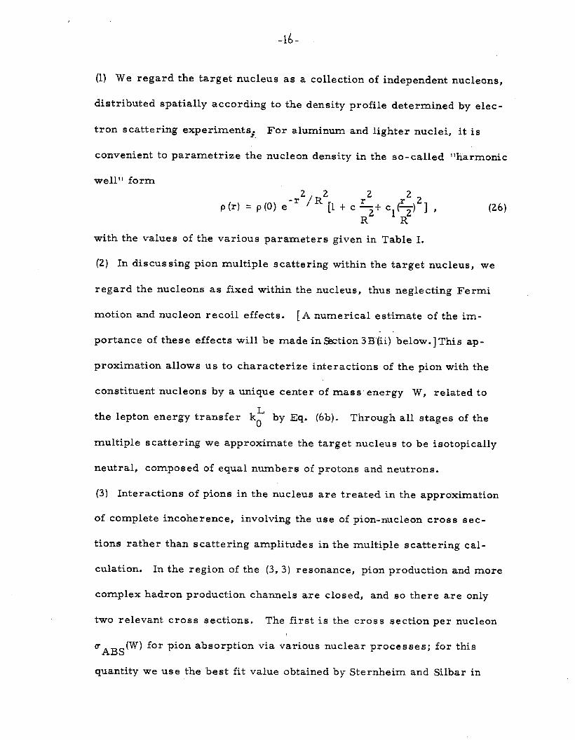
‘(1) We regard the target nucleus as a collection of independent nucleons,

distributed spatially according to the density profile determined by elec-

tron scattering experiments, -_ For aluminum and lighter nuclei, it is

convenient to parametrize the nucleon density in the so-called “harmonic

well” form

p(r) = ~10) e -r2/R2[l t c 5 Cl(?) ] , 22

R2 R (26)

with the values of the various parameters given in Table I.

(2) In discussing pion multiple scattering within the target nucleus, we

regard the nucleons as fixed within the nucleus, thus neglecting Fermi

motion and nucleon recoil effects. [A numerical estimate of the im-

portance of these effects will be made in &&ion 3B’(ii) below.] This ap-

proximation allows us to characterize interactions of the pion with the

constituent nucleons by a unique center of mass energy W, related to

the lepton energy transfer k by Eq. (6b). Through all stages of the

multiple scattering we approximate the target nucleus to be isotopically

neutral, composed of equal numbers of protons and neutrons.

(3) Interactions of pions in the nucleus are treated in the approximation

of complete incoherence, involving the use of pion-nucleon cross sec-

tions rather than scattering amplitudes in the multiple scattering cal-

culation. In the region of the (3, 3) resonance, pion production and more

complex hadron production channels are closed, and so there are only

two relevant cross sections. The first is the cross section per nucleon

uABS(W) for pion absorption via various nuclear processes; for this

quantity we use the best fit value obtained by Sternheim and Silbar in

-17-

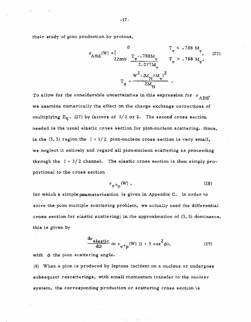
their study of pion production by protons,

0 UABSW) ={.

T.,, < .788 M IT

T 22mb TT

-. 788M

2. 077Mm Tn > 0788 M ;

(27)

IT IT

T = W2- (MN+MJ2

Tr 2MN l

To allow for the considerable uncertainties in this expression for u ABS’

we examine .numerically the effect on the charge exchange corrections of

multiplying Eq . (27) by factors of l/2 or 2. The second cross section

needed is the usual elastic cross section for pion-nucleon scattering. Since,

in the (3,3) region the I = l/ 2 pion-nucleon cross section is very small,

we neglect it entirely and regard all pion-nucleon scattering as proceeding

through the I = 3/Z channel. The elastic cross section is then simply pro-

portional to the cross section

“,fpW) , (28)

for which a simple~meterization is given in Appendix C. In order to

solve the pion multiple scattering problem, we actually need the differential

cross section for elastic scattering: in the approximation of (3, 3) dominance,

this is giv,en by

da elastic dS2 Oc ?r+p (W) (1 t 3 cos2q5), (29)

with Q1 the pion scattering angle.

(4) When a pion is produced by leptons incident on a nucleus or undergoes

subsequent rescatterings, with small momentum transfer to the nuclear

system, the corresponding production or scattering cross section is

-18-

reduced by the Pauli exclusion principle. 7

We take this effect into ac-

count,within the framework of the independent nucleon picture, by multiply-

ing the lepto-pion production cross section and the pion nucleon rescattering

cross section by respective reduction factors g(W, k‘) and h(W, $). Form-

ulas for these factors are given in Appendix C. Neutrino quasielastic scat-

tering experiments at small momentum transfer k2 provide some empirical

evidence for the presence of the production factor g. The argument for in-

cluding h is less compelling, since we are using a semiclassical picture,

with fixed constituent nucleons, for treating the pion multiple scattering in

the nuclear medium, and in a semiclassical picture there are no Pauli ef-

fects. To take this objection 13

into account, in the numerical work below

we also calculate results for the case in which h is replaced by unity.

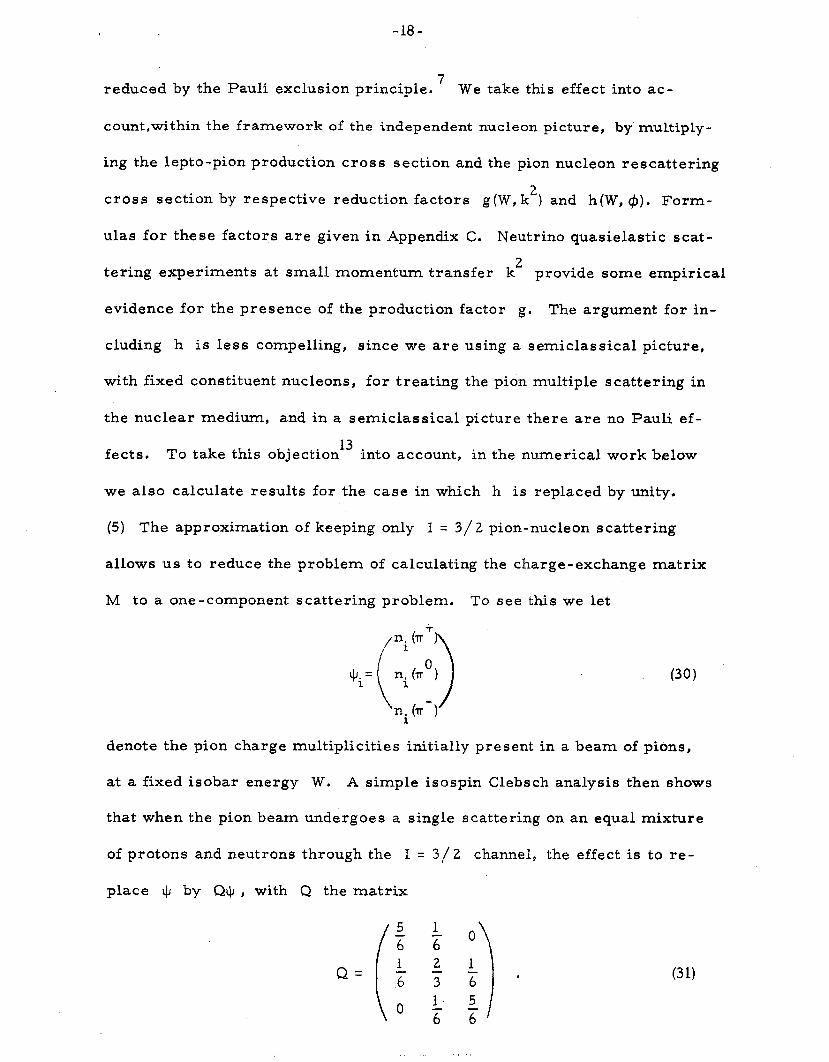
(5) The approximation of keeping only I = 3/2 pion-nucleon scattering

allows us to reduce the problem of calculating the charge-exchange matrix

M to a one-component scattering problem. To see this we let

4.

(30)

denote the pion charge multiplicities initially present in a beam of pions,

at a fixed isobar energy W. A simple isospin Clebsch analysis then shows

that when the pion beam undergoes a single scattering on an equal mixture

of protons and neutrons through the X = 3/2 channel, the effect is to re-

place 4 by Q+ , with Q the matrix

1 a 2 3

1 6

0

1 a * 5 a 1

(31)

-19-

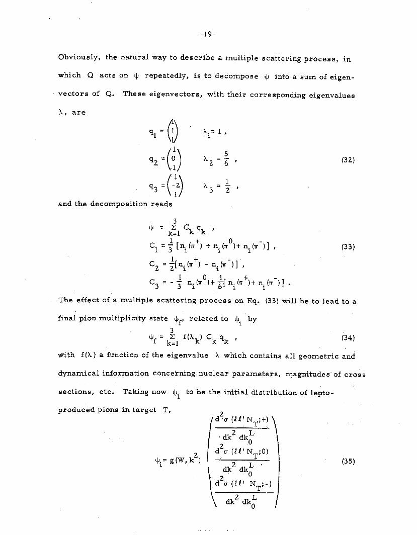
Obviously, the naturai way to describe a multiple scattering process, in

which Q acts on L/J repeatedly, is to decompose $ into a sum of eigen-

vectors of Q. These eigenvectors, with their corresponding eigenvalues

A, are 1

q1= 0 1 Al= 1 )

1 q2= 0 0

1 x2=;,

1 0 -2

1 q3=

1 x3=?,

(32)

and the decomposition reads

+ = k’l ‘k qk 9 = cl = 3 [ni h+) t nib’)+ nih-)l 9 (33)

c2 = -$ni(r+) - ni(r-)l ‘B

c3 = - f ni(nD)t j$ ni(r+)+ ni(T-)l l

The effect of a multiple scattering process on Eq. (33) will be to lead to a

final pion multiplicity state Qf, related to Jli by

+, = k$ f(kk) ‘k qk , (34)

with f(X) a function of the eigenvalue X which contains all geometric and

dynamical information concekningrnuclear parameters, magnitudes’ of cross

sections, etc. Taking now $i to be

produced pions in target T,

le initial distribution of lepto-

d20- (41’ N,; t) ’

$;= g (W, k2)

. dk2 dk;

d2a (11; NT;O)

2 Id* dk. dko. d2ii-(W N

T ’ ;-

(35)

-2o-

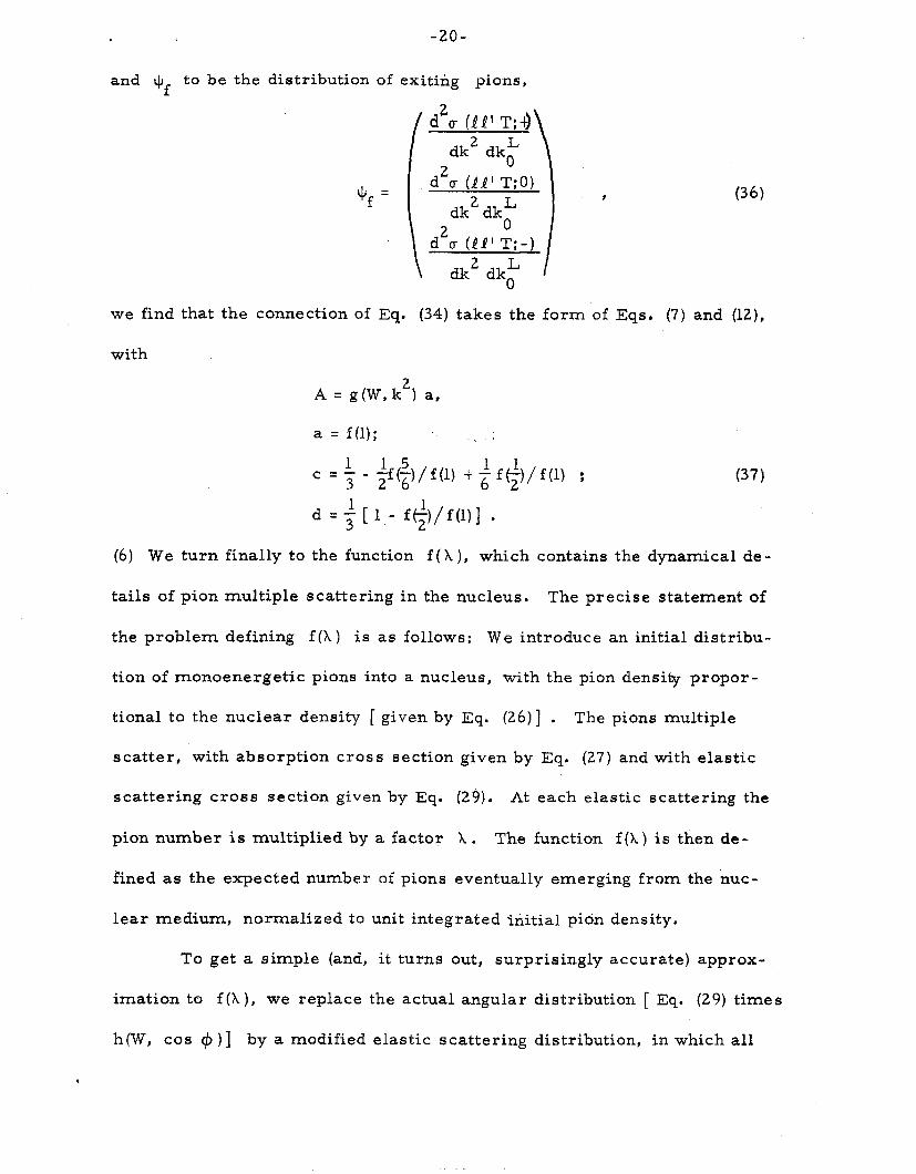
and + f

to be the distribution of exiting pions,

d2c (.W T;+)\ dk2 dkt

d2a (11’ T;O) \

dk2 dk;

d2cr (11’ T;-)

dk2 dkt

(36)

we find that the connection of Eq. (34) takes the form of Eqs. (7) and (12),

with

A = g(W,k2) a,

a = f(1); _. ;

c = 3 - $+/f(l) t ; f($/f(l) : (37)

d = 3 [ 1 - f(;)/f(l)l l

(6) We turn finally to the function f (X ), which contains the dynamical de-

tails of pion multiple scattering in the nucleus. The precise statement of

the problem defining f(X) is as follows: We introduce an initial distribu-

tion of monoenergetic pions into a nucleus, with the pion density propor-

tional to the nuclear density [ given by Eq. (26)] . The pions multiple

scatter, with absorption cross section given by Eq. (27) and with elastic

scattering cross section given by Eq. (29}. At each elastic scattering the

pion number is multiplied by a factor h. The function f (h ) is then de -

fined as the expected number of pions eventually emerging from the nuc-

lear medium, normalized to unit integrated initial pidn density.

To get a simple (and, it turns out, surprisingly accurate) approx-

imation to f(h), we replace the actual angular distribution [ Eq. (29) times

h(W, cos $I )] by a modified elastic scattering distribution, in which all

u

-21-

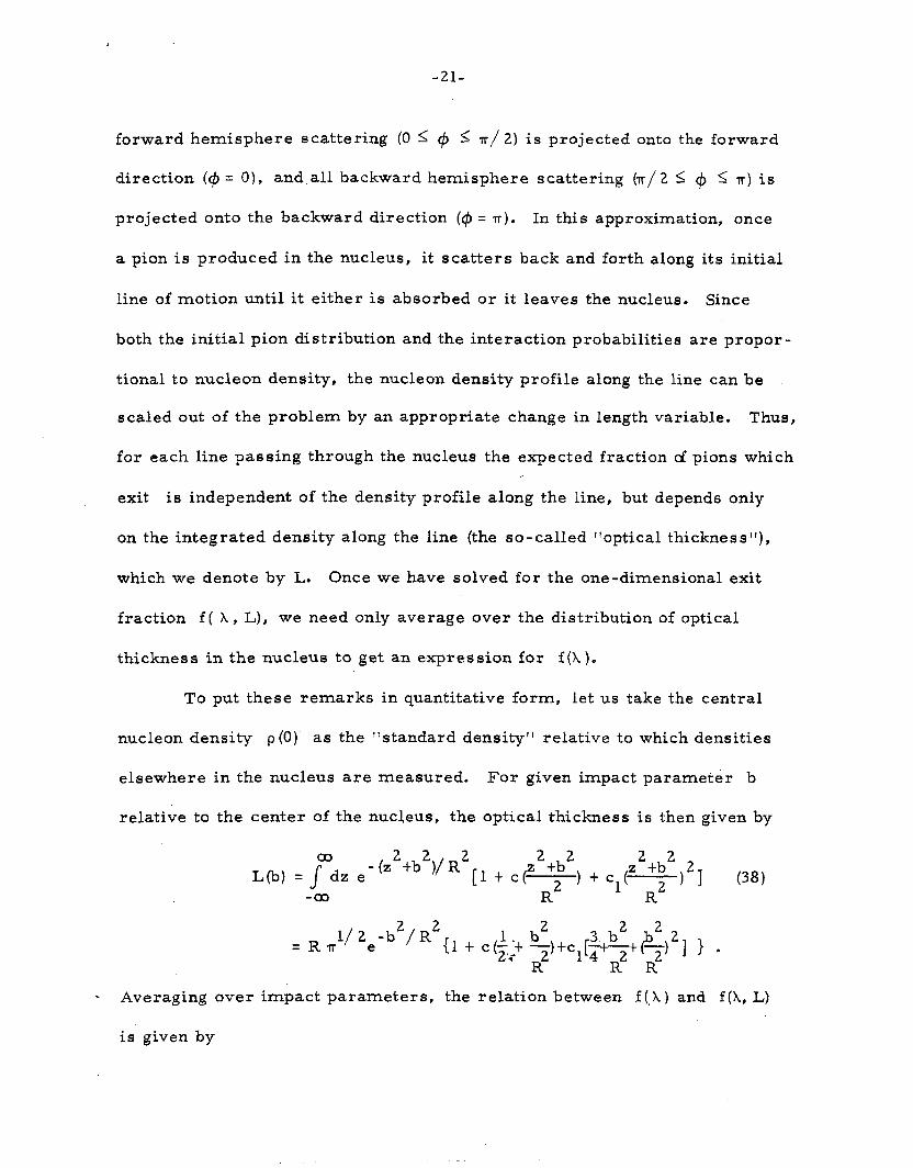
forward hemisphere scattering (0 I I$ I n/ 2) is projected onto the forward

direction (# = 0), and all backward hemisphere scattering (n/ 2 <_ $ I TT) is

projected onto the backward direction (lp = r). In this approximation, once

a pion is produced in the nucleus, it scatters back and forth along its initial

line of motion until it either is absorbed or it leaves the nucleus. Since

both the initial pion distribution and the interaction probabilities are propor-

tional to nucleon density, the nucleon density profile along the line can be

scaled out of the problem by an appropriate change in length variable. Thus,

for each line passing through the nucleus the expected fraction $ pions which

exit is independent of the density profile along the line, but depends only

on the integrated density along the line (the so-called “optical thickness”),

which we denote by L. Once we have solved for the one-dimensional exit

fraction f( A, L), we need only average over the distribution of optical

thickness in the nucleus to get an expression for f(h).

To put these remarks in quantitative form, let us take the central

nucleon density p (0) as the “standard density” relative to which densities

elsewhere in the nucleus are measured. For given impact parameter b

relative to the center of the nucleus, the optical thickness is then given by

2 2 I = Jmdz e-(z2+b2)~R2[~ $ (” +b

2 2 c -) t cl(--)2]

-m R2 R2 (38)

= R ,$2e-b2/R2{l + c(-$ 2.i

. Averaging over impact parameters, the relation between f (,X) and f(X, L)

is given by

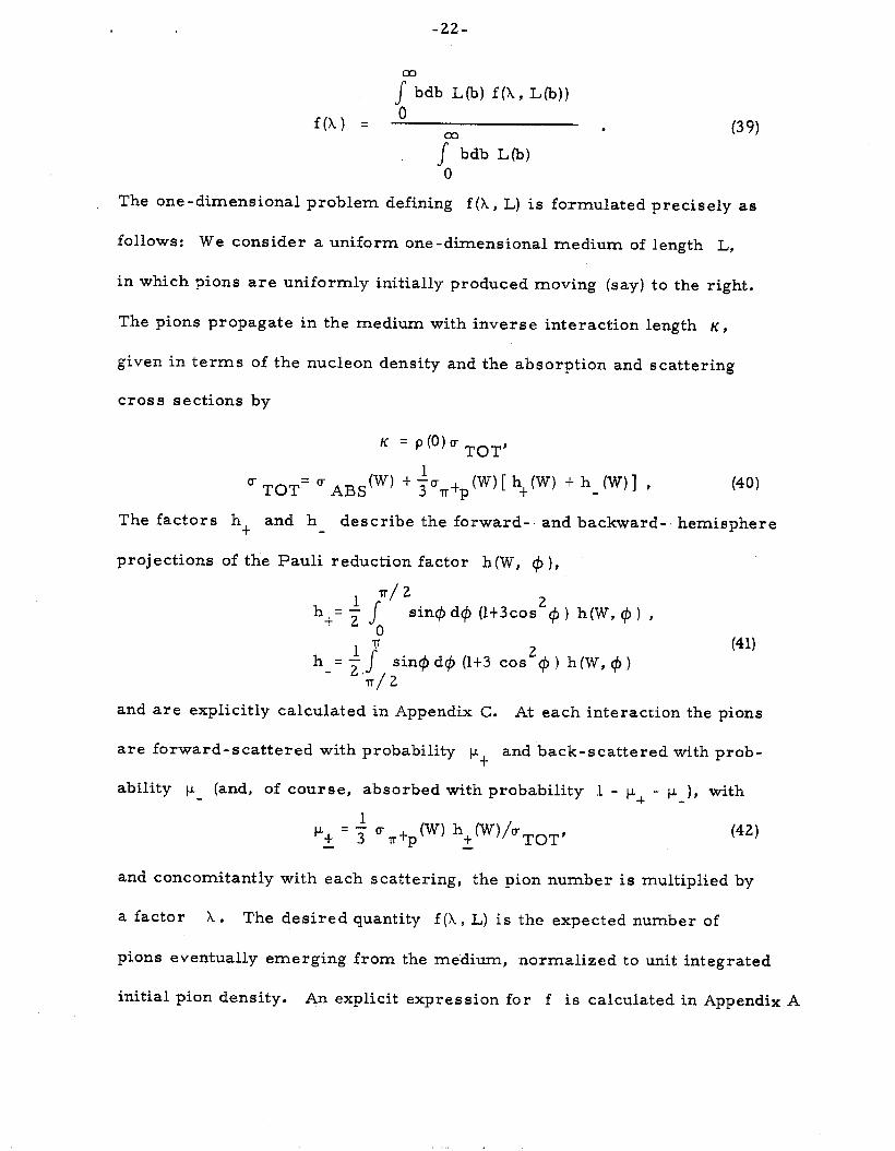
-22-

03

s bdb Lb) f(h, L(b))

f(h) = * . a3 (39)

s bdb L(b) 0

The one-dimensional problem defining f(X, L) is formulated precisely as

follows: We consider a uniform one-dimensional medium of length L,

in which pions are uniformly initially produced moving (say) to the right.

The pions propagate in the medium with inverse interaction length K,

given in terms of the nucleon density and the absorption and scattering

cross sections by

K = pt”hTOT

1 O- TOT= F ABS (W) + yrtp (W) [ ht (W + h- W 1 ,

The factors ht and h describe the forward-. and backward-. hemisphere

projections of the Pauli reduction factor h(W, $I),

r/2 ht= + $ sin$dql (1t3cos2$) h(W, #) ,

0

h-= $J sin$d$ (lt3 cos’$) h(W, C#I) ‘3-r/ 2

(41)

and are explicitly calculated in Appendix C. At each interaction the pions

are forward-scattered with probability pt and back-scattered with prob-

ability t-~ (and, of course, absorbed with probability 1 - pLt- - p ), with

and concomitantly with each scattering, the pion number is multiplied by

a factor h. The desired quantity f(h, L) is the expected number of

pions eventually emerging from the medium, normalized to unit integrated

initial pion density. An explicit expression for f is calculated in Appendix A

-23-

[ $jee Eq. (A. 12) and Eqs. (A. 25) - (A, 27)] , as well as expressions for

ft and f , the expected fractions of pions eventually emerging with and

without a net reversal of direction of motion along the line. In Appendix B

we compare the approximate solution for f(h) given by Eq. (39) with the

exact solution in the simple geometry of a uniform sphere composed of

material which scatters isotropically, and find very satisfactory agree-

ment. Since the actual angular distribution of interest to us, 1 t 3 cos2G,

is already peaked in the backward and forward directions, 14

our approx-

imation should be at least as accurate for this case as it is for handling

isotropic scattering.

This completes the specification of our multiple scattering model.

As we have already noted, it closely resembles the calculation of

Sternheim and Silbar, and the reader is referred to Ref. 3 for an excellent,

detailed analysis of the approximations and physical assumptions which are

involved. The aspects in which our model differs from that of Ref. 3 are:

(1) We take into account the diffuseness of the nuclear edge, rather than

treating the nucleon distribution as a uniform sphere; (2) We take Pauli

exclusion effects into account in a crude way: and (3) We use an improved

approximation for solving the pion multiple-scattering problem. Instead

of using the back-forward approximation described above, Sternheim and

Silbar use the considerably less accurate approximation of treating all

scattering as purely forward scattering. A comparison of their approx-

imation with the exact solution, in the case of a uniform sphere com-

posed of material which scatters isotropically, is given in Appendix B,

-24-

B. Numerical Calculations

We turn now to numerical calculations, in which we combine our

model for nuclear charge-exchange corrections with the theory of pion

electro- and weak production from free nucleon targets developed in

Ref. 5. For the hadronic weak neutral current, we adopt the Weinberg-

model form 15

A3 j;eutr$~;3$ Jx -2 sin2 O,wJTmi (43)

. we will say a few words below about variants of this model in which Eq.

(43) contains an additional isoscalar current. We assume throughout an

incident lab neutrino energy L k10 = 1 GeV and a nucleon elastic form factor’

p,oA = 1. 24

&j k2 1’ ’ L (0. 9 GeV/c)zl

(44)

and take integrations over the (3, 3)-resonance region to extend from the

pion production threshold up to a maximum isobar mass of W = 1.47 GeV.

In our calculations on aluminum, we weight the free nucleon production

cross sections according to the actual neutron/proton ratio in aluminum

[ i. e., we take N T= 13p $ 14n] , but as emphasized above, we

adopt the approximation of isotopic neutrality in calculating charge ex-

change corrections.

(if Calculation of R’ from Eq. (15) (with Fermi motion neglected)

In Table II we present results for the ratio RI on an aluminum

target, calculated by using Eq. (15) to fold the W-dependent charge ex-

change matrix into the production cross sections from a free nucleon

target at rest [ i. e., we neglect the Fermi-motion average symbolized

-25-

by the subscript ‘IF” in Eq. (15)] . In the second column we tabulate

u(v SN R(NT) =

T -v +N~~IT*)

-p-t N’,;, t a*) * (45)

2a (vp •t NT

which is the ratio predicted by the production model when no charge-ex-

change corrections are made. In the third through seventh columns we

tabulate values of the charge-exchange-corrected ratio R’ obtained under

various alternative assumptions. The column labeled “No variations” is

the result obtained from the multiple scattering model of Sec. 3A above;

the next three columns show how this result changes when the Pauli factors

h in Eqs. (40) and (42) are replaced by unity, or when the absorption cross

section of Eq. (27) is modified. The predictions for R’ are evidently

quite insensitive to these variations. The seventh column gives the result

for RI when all isoscalar multiples are omitted. Since the isoscalar

multipoles only contribute quadratically to R’ p 16

this column gives a

lower bound on R’ for any variant of the Weinberg theory in which the

hadronic neutral current differs from Eq. (43) by purely isoscalar terms.

in the final column we have used our production and charge exchange cal-

culations to generate simulated pion weak and electroproduction cross

sections on aluminum, which are then used to evaluate the lower bound

on Rf derived by Albright et., al. 17 in the isos calar -target approximation,

R’ (13A127) + { [ F( V A127)-l]’ -2 sin% r v*

pp-13

,i )

em 1 12.

w 1-u (~~p-~~A~~~:o)l

Y(v p- ~ 13A127) = UW P-~~A~

27 ;t) + UIV P-~~A~ 27 ;- ) n (46)

o- (vpP- 13 A127 ;*I

-26-

+* G2cos2 13 c 1 du (eelgAl 27;o)

= 0 em l-r

4T cY2 s (‘k2)2 dk2

dk2

We see that the bound of Eq. (46) provides a satisfactory estimate of R’

for small values of sin2Qw.

We turn next to Table III, where we have tabulated charged pion

to neutral pion production ratios for the usual charged weak current.

The first column gives the standard 5:l prediction for an isotopically

neutral target, assuming complete I = 3/Z dominance. When 1=1/2

multipoles are taken into account, 18 the prediction is lowered to 3.67:1,

as shown in the second column., Finally, in the third column we give

the prediction of 2.63:1 which results when Eq. (15)* and its analog for

charged pions, are used to fold in charge-exchange corrections for alum-

inum. 19 It would obviously be very desirable to try to check this pre-

diction for G simultaneously with the experimental determination of R’ .

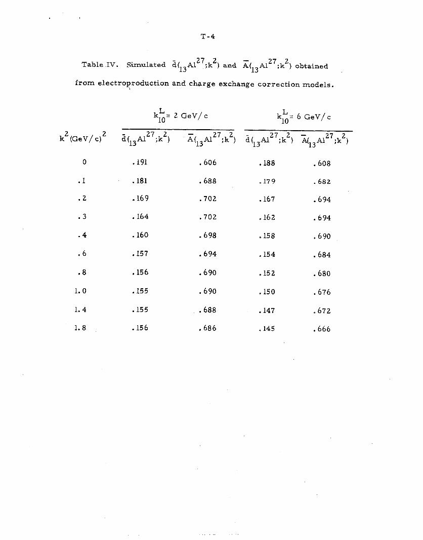
(ii) Averaging approximations, comparison of different nuclei and

estimate of nucleon motion effects+

We conclude with a test of the averaging approximations intro-

duced in Sec. 2 and a discussion of related topics. To study Eqs. (20)-(23),

we fold together the electroproduction and charge exchange models, as

in Eq. (15), ,to give simulated data for pion electroproduction cross sec-

tions on aluminum. Substituting this data into Eqs. (21) and (22) then

gives the values for ‘;i and x tabulated in Table IV. The charge ex-

change parameters obtained this way are seen to be nearly independent

L of the incident electron energy kloJ and are slowly varying functions of

-27-

k2 except in the region k2 5 .3, where Pauli exclusion effects and I = l/ 2

multipoles arising from the pion exchange graph become important. Sub - -

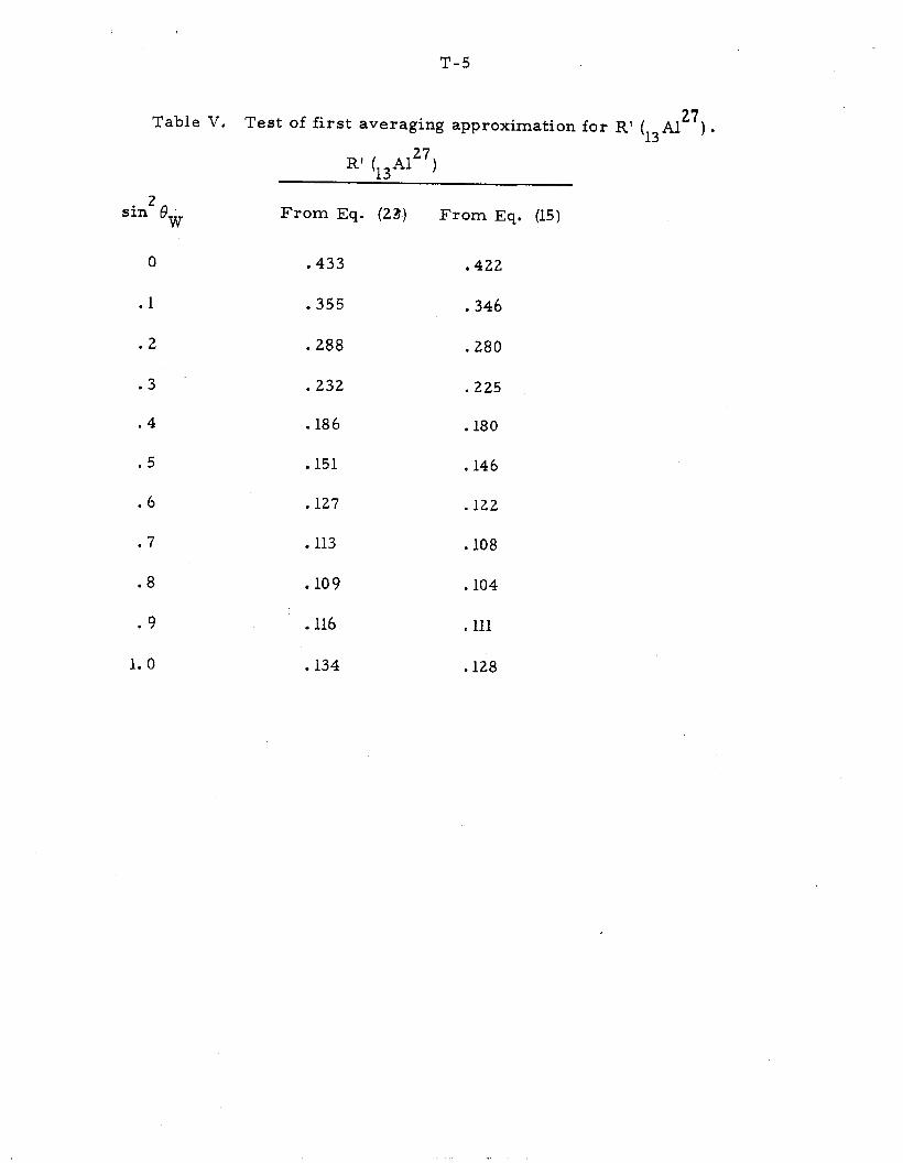
stituting the 2 GeV/ c values of d and A into Eq. (23), and continuing to

use our production model for the neutrino cross sections, gives the values

of R’ tabulated in the second column of Table V. In the third column we

transcribe from Table II the values of R1 obtained directly from Eq. (15);

the good agreement indicates that the averaging approximation is working.

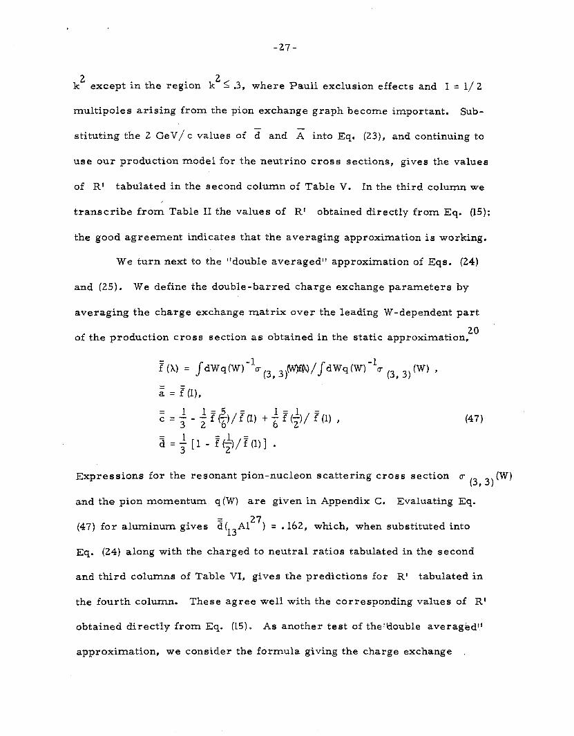
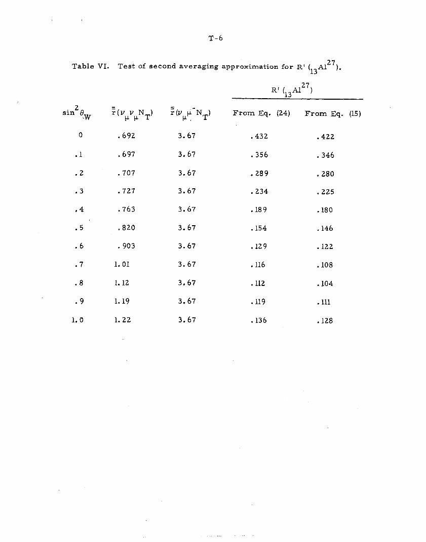
We turn next to the “double averaged” approximation of Eqs. (24)

and (25). We define the double-barred charge exchange parameters by

averaging the charge exchange matrix over the leading W-dependent part

of the production cross section as obtained in the static 20

approximation,

f=(1) = sdWq(W)% (3, ,)MYN/JdWq(W) -+ (3, 3) (W) ’

ii = f(l),

1 &-. 3

- + T{#l, t i f(i)/ T(l) )

2i = f [1 - I(j/I(l)] .

(47)

Expressions for the resonant pion-nucleon scattering cross section u (3, 3)(w)

and the pion momentum q(W) are given in Appendix C. Evaluating Eq.

(47) for aluminum gives a(13A127) = e 162, which, when substituted into

Eq. (24) along with the charged to neutral ratios tabulated in the second

and third columns of Table VI, gives the predictions for R’ tabulated in

the fourth column. These agree well with the corresponding values of RI

obtained directly from Eq. (15), As another test of the’tiouble averagedt,l

approximation , we consider the formula giving the charge exchange ,

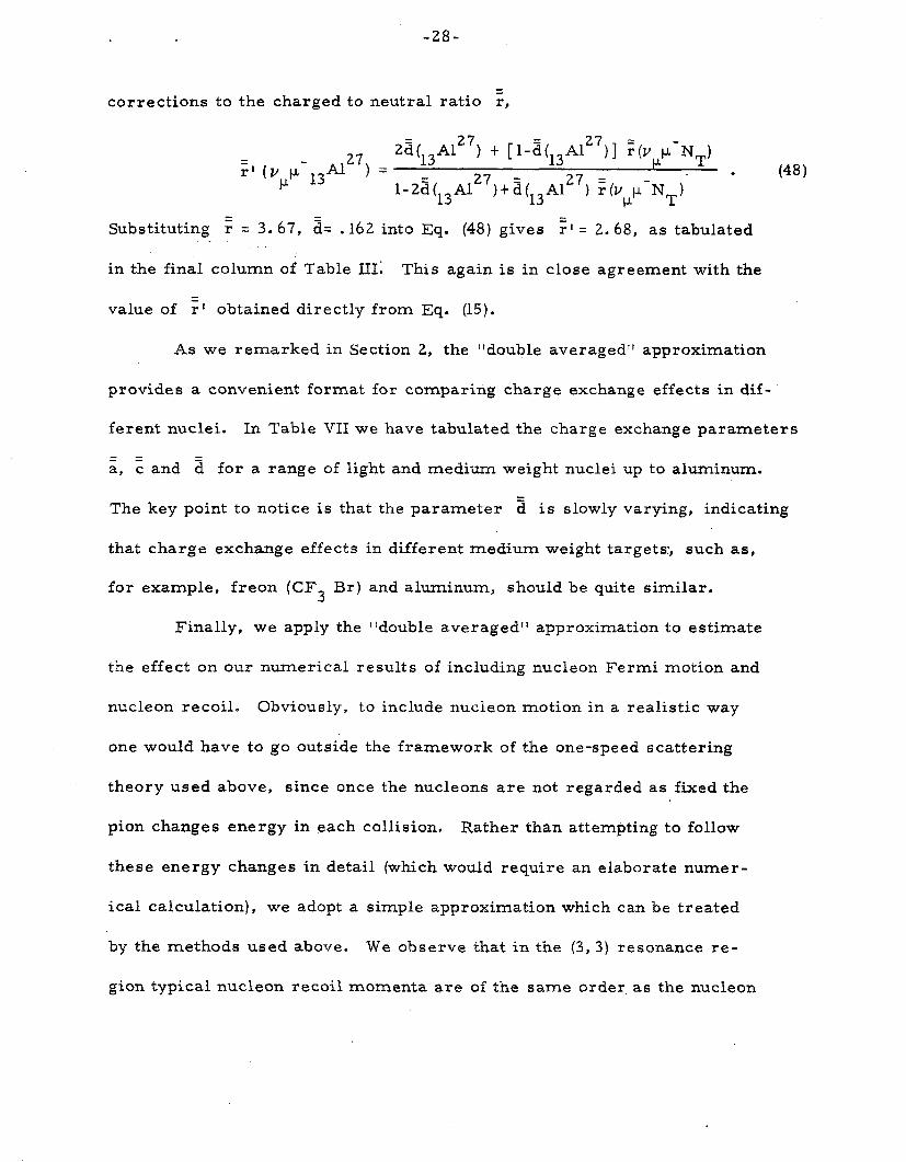
-28-

corrections to the charged to neutral ratio r,

27 :I ( vppj3Al ) =

2d(13A127) t [1-$(13A127)] :(v p-NT)

1-2;(13A127)+ a(13A1Z7) F @i-NT)- .

Substituting F = 3.67, z= .162 into Eq. (48) gives it = 2.68, as tabulated

in the final column of Table 111. This again is in close agreement with the

value of ;I obtained directly from Eq. (15).

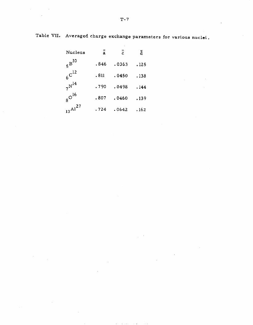
As we remarked in Section 2, the “double averaged” approximation

provides a convenient format for comparing charge exchange effects in dif-

ferent nuclei. In Table VII we have tabulated the charge exchange parameters

:, = c and a for a range of light and medium weight nuclei up to aluminum.

The key point to notice is that the parameter a is slowly varying, indicating

that charge exchange effects in different medium weight targets:, such as,

for example, freon (CF3 Br) and aluminum, should be quite similar.

Finally, we apply the “double averaged” a pproximation to estimate

the effect on our numerical results of including nucleon Fermi motion and

nucleon recoil. Obviously, to include nucieon motion in a realistic way

one would have to go outside the framework of the one-speed scattering

theory used above, since once the nucleons are not regarded as fixed the

pion changes energy in each collision. Rather than attempting to follow

these energy changes in detail (which would require an elaborate numer-

ical calculation), we adopt a simple approximation which can be treated

by the methods used above. We observe that in the (3,3) resonance re-

gion typical nucleon recoil momenta are of the same order as the nucleon

-29-

Fermi momentum (~1.6 M,/ c); hence a rough estimate of nucleon recoil

and Fermi motion effects should be given by the simple randomizing ap-

proximation of regarding the pion energy as a constant throughout its mo-

tion in the nucleus, but replacing the pion production and charge exchange

scattering cross sections by corresponding cross sections which are

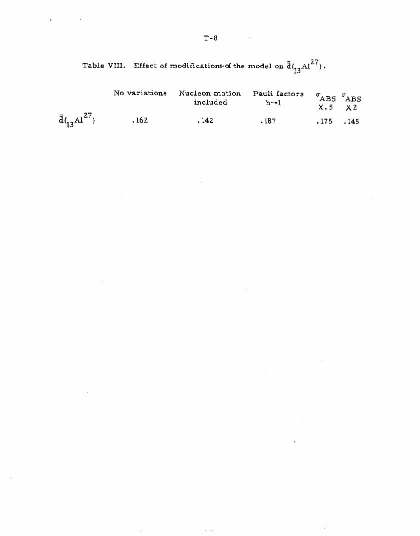
smeared over nucleon Fermi motion. Evaluating Eq. (47) using these

smeared cross sections gives g(13A127) = .142, as compared with the

value of .162 which results when nucleon motion is neglected. We see

that the change in 2 is relatively small, and is in the direction of re-

ducing the size of charge exchange effects; we expect these qualitative .

features to survive in a more careful treatment of nucleon motion effects.

In Table VIII we 27

sumrn arize the values of d(l,Al ) obtained in our orig-

inal model and when various modifications are made.

C. Pion Angular Distributions

Up to this point we have only discussed charge exchange correc-

tions to cross sections in which the pion angular variables have been

integrated out. Our model, however, makes specific predictions for

angular distributions as well, and although they are much more subject

to error than the integrated predictions, 21

they are essential for des-

cribing experimental situations in which the pion acceptance is limited.

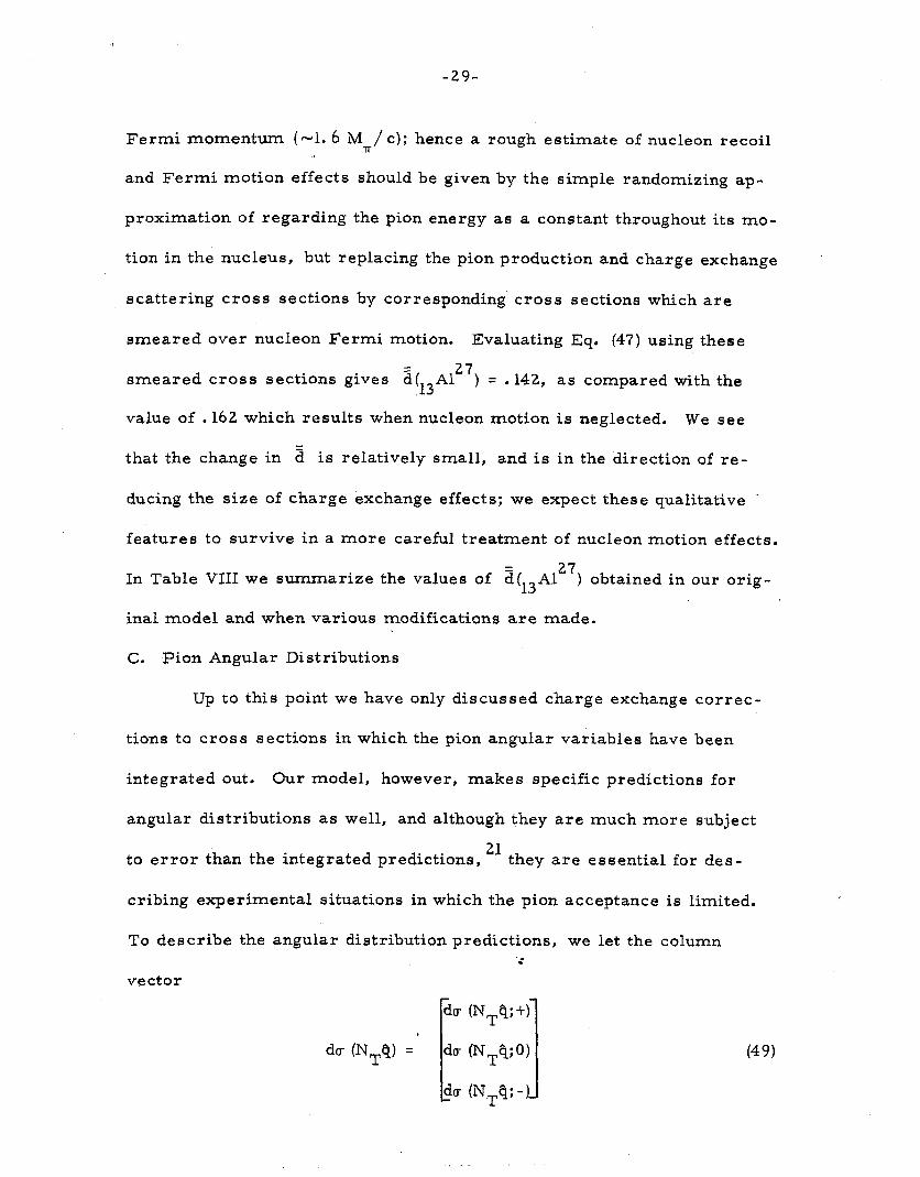
To describe the angular distribution predictions, we let the column ‘i

vector

r du (NTq;tj

da (NTq) = (49)

-3o-

denote the free-nucleon-target pion production cross section, with the

pion emerging in direction Q. In the back-forward scattering approxi-

mation, after undergoing nuclear interactions the pion can either emerge

in direction 21 or can emerge with reversed direction -Q*

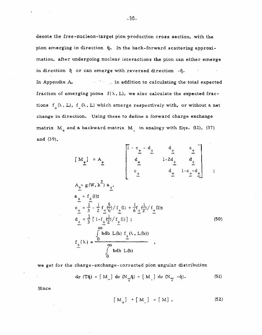
In Appendix A,, ‘: ; in addition to .calculating the total expected

fraction of emerging pions f (X, L), we also calculate the expected frac-

tions f+ (X 9 L), f (X, L) which emerge respectively with, or without a net

change in direction. Using these to define a forward charge exchange

matrix M+ and a backward matrix M in analogy with Eqs. (12), (37)

and (391,

A+= g (W, k2) a+, -

a+ = f+(l):

1- 1 =-- %3 _ y f+($/ft(l) -t $+&fp:

d; = f [ l-fi($/f;(l)] ; - -

co

s f+(X) = O

bdb Lb) f,(L Lb))

al , -

s bdb L(b) 0

(50)

we get for the charge-exchange-corrected pion angular distribution

dr (Ta) = [ M+] do (NTQ) + [ M ] dF (NT -$I* (511

Since

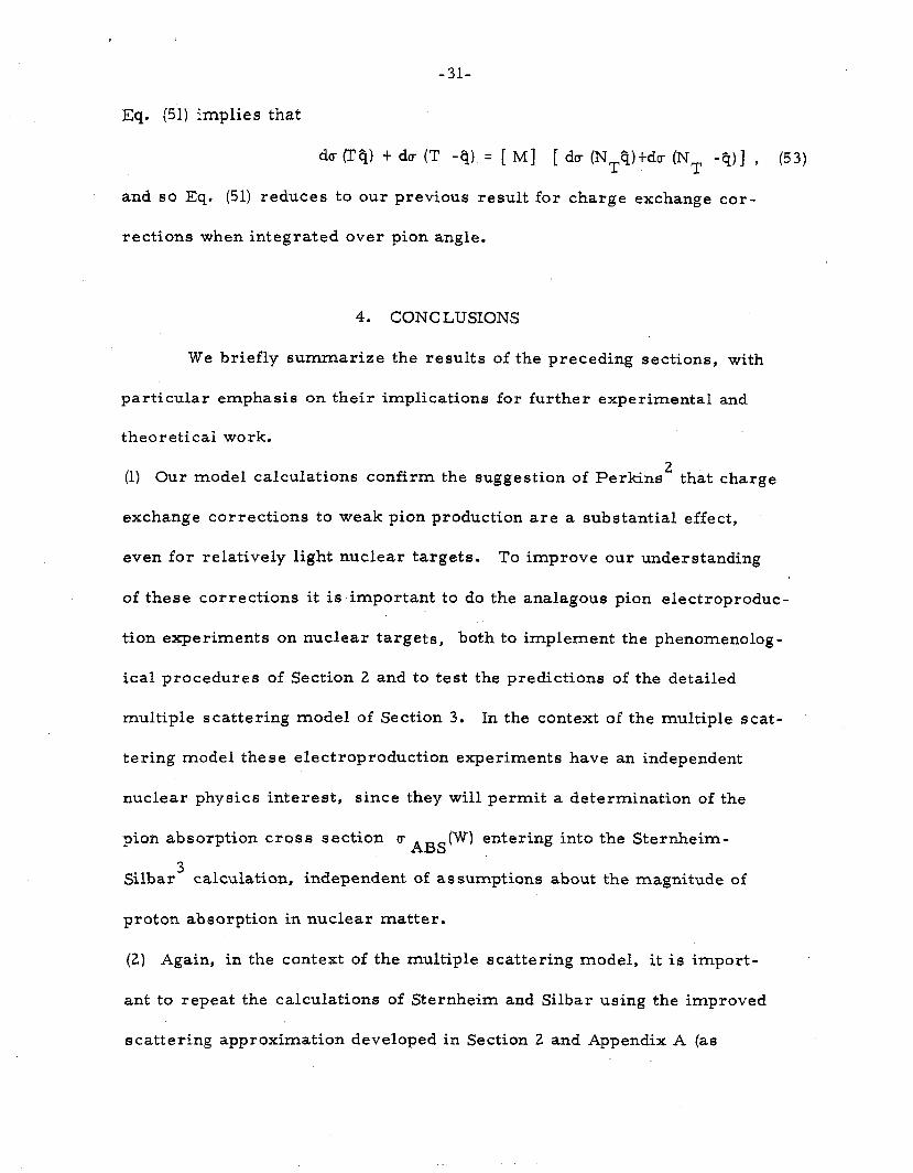
[M+l -+[M-1 =[Ml, (52)

-31-

Eq. (51) implies that

du (I$) t do (T -$) = [ M] [ du (NTQfdu (NT -q)] , (53)

and so Eq. (51) reduces to our previous result for charge exchange cor-

rections when integrated over pion angle.

4. CONCLUSIONS

We briefly summarize the results of the preceding sections, with

particular emphasis on their implications for further experimental and

theoretical work.

(1) Our model calculations confirm the suggestion of Perkins 2

that charge

exchange corrections to weak pion production are a substantial effect,

even for relatively light nuclear targets. To improve our understanding

of these corrections it is important to do the analagous pion electroproduc-

tion experiments on nuclear targets, both to implement the phenomenolog-

ical procedures of Section 2 and to test the predictions of the detailed

multiple scattering model of Section 3. In the context of the multiple scat-

tering model these electroproduction experiments have an independent

nuclear physics interest, since they will permit a determination of the

pion absorption cross section uABS (W) entering into the Sternheim-

Silbar3 calculation, independent of assumptions about the magnitude of

proton absorption in nuclear matter.

(2) Again, in the context of the multiple scattering model, it is import-

ant to repeat the calculations of Sternheim and Silbar using the improved

scattering approximation developed in Section 2 and Appendix A (as

-32-

extended 9

to the case of a neutron excess). This will permit the extraction

of an optimized pion absorption cross section u Ass(W) appropriate to the

precise model which we use, and hopefully, may reduce some of the remain- +.

ing areas of disagreement between the Sternheim-Silbar calculation and

experiment.

(3) Our calculations suggest that the ratio R’ (13A127) is larger than a-

bout .18 when the Weinberg parameter is in the currently interesting2 range

sin’ t9 w5 l

35. We do not attach great significance to the fact that this

theoretical estimate of Rt exceeds the upper bound of .14 reported by

W. Lee,l since the discrepancy is easily of the order of uncertainties in

the predictions of our production and charge-exchange models. We be-

lieve that a reasonably conservative statement is that if the hadronic neu-

tral weak current has (up to isoscalar additions) the form of Eq. (43), and

if sin2ew < . 35, then R’ N on an aluminum target is in the neighborhood

of a fifteen percent effect. Thus, an experiment capable of measuring R’

to a level of a few percent will provide a decisive test of Eq. (43), and if

Eq. (43) is correct, should permit a crude determination of sin28 W’

ACKNOWLEDGEMENTS

We wish to thank C. Baltay, M.A. B. Beg, K.M. Case, L. Hand,

A. K.erman, B. W. Lee, W. Lee, H. J. Lipkin, S. B. Treiman and J. D.

Walecka for helpful conversations. One of us (S. L. A. ) wishes to acknow-

ledge the hospitality of the Aspen Center for physics, where initial parts

of this work were done.

A-l

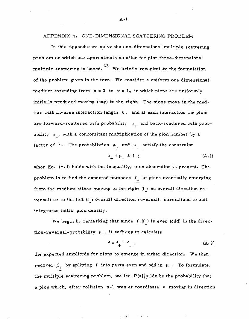
APPENDIX A. ONE-DIMENSIONAL SCATTERING PROBLEM

In this Appendix we solve the one-dimensional multiple scattering

problem on which our approximate solution for pion three-dimensional

multiple scattering is based. 22

We briefly recapitulate the formulation

of the problem given in the text, We consider a uniform one dimensional

medium extending from x = 0 to x = L, in which pions are uniformly

initially produced moving (say) to the right. The pions move in the med-

ium with inverse interaction length K, and at each interaction the pions

are forward-scattered with probability p+ and back-scattered with prob-

ability p , with a concomitant multiplication of the pion number by a

factor of X. The probabilities t.~+ and p satisfy the constraint

Pt + P- 5 1 ; (A. 1) when Eq. (A. 1) holds with the inequality, pion absorption is present. The

problem is to find the expected numbers $ of pions eventually emerging

from the medium either moving to the right (f+: no overall direction re-

versal) or to the left (f : overall direction reversal), normalized to unit

integrated initial pion density.

We begin by remarking that since ft(f ) is even (odd) in the direc-

tion-reversal-probability p , it suffices to calculate

f=f+$f ,

the expected amplitude for pions to emerge in either direction. We then

recover f+ by splitting f into parts even and odd in p e To formulate

the multiple scattering problem, we let P(xj 1 yi)dx be the probability that

a pion which, after collision n-l was at coordinate y moving in direction

A-2

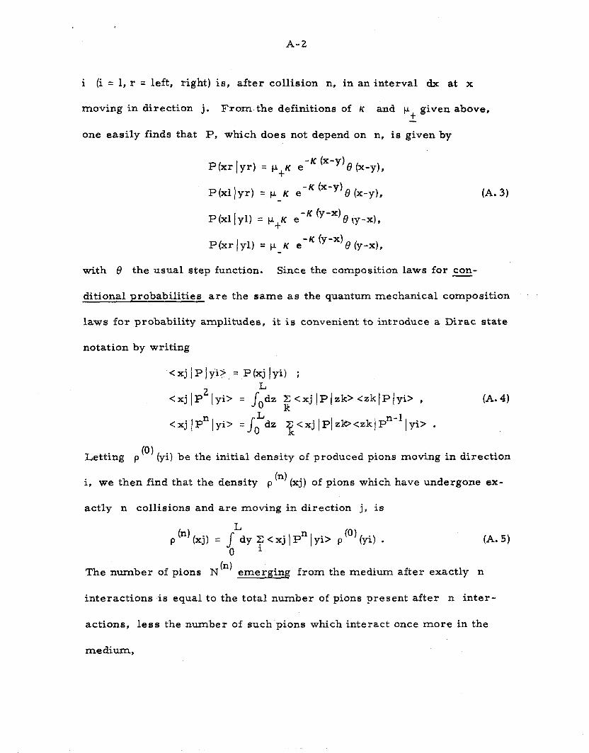
i (i=l,r = left, right) is, after collision n, in an interval dx at x

moving in direction j. From. the definitions of ic and p+ given above,

one easily finds that P, which does not depend on n, is given by

P(xrlyr) = p+K e -K (x-y) 0 (x-y),

P(xl]yr) = p K e -K tx-y+j (x-y),

P(xllyl) = p+K e -K (y-x)

8 \y-4,

P(xr(yl) = p K e -K (y-x)(J (y-x),

(A. 3)

with 0 the usual step function. Since the composition laws for con-

ditional probabilities are the same as the quantum mechanical composition 1

laws for probability amplitudes, it is convenient to introduce a Dirac state

notation by writing

<xjlPJyiT,= P(xj./yi) ; L

<xj (P2 lyi> = JOdz $ <xj [P(zk> <xklP(yi> , (A. 4)

<xj !Pn/yi> =JOLdz E<xj IPlz*<zkjPnWIIyi> .

Letting p (O) (yi) be the initial density of produced pions moving in direction

i, we then find that the density p (4 (xj) of pions which have undergone ex-

actly n collisions and are moving in direction j, is

$n) L

(xj) = $ dy F<xj\Pn/yi> p(‘)(yi) . (A. 5) 0

The number of pions N (n) emerging from the medium after exactly n

interactions is equal to the total number of pions present after n inter-

actions, less the number of such pions which interact once more in the

medium,

A-3

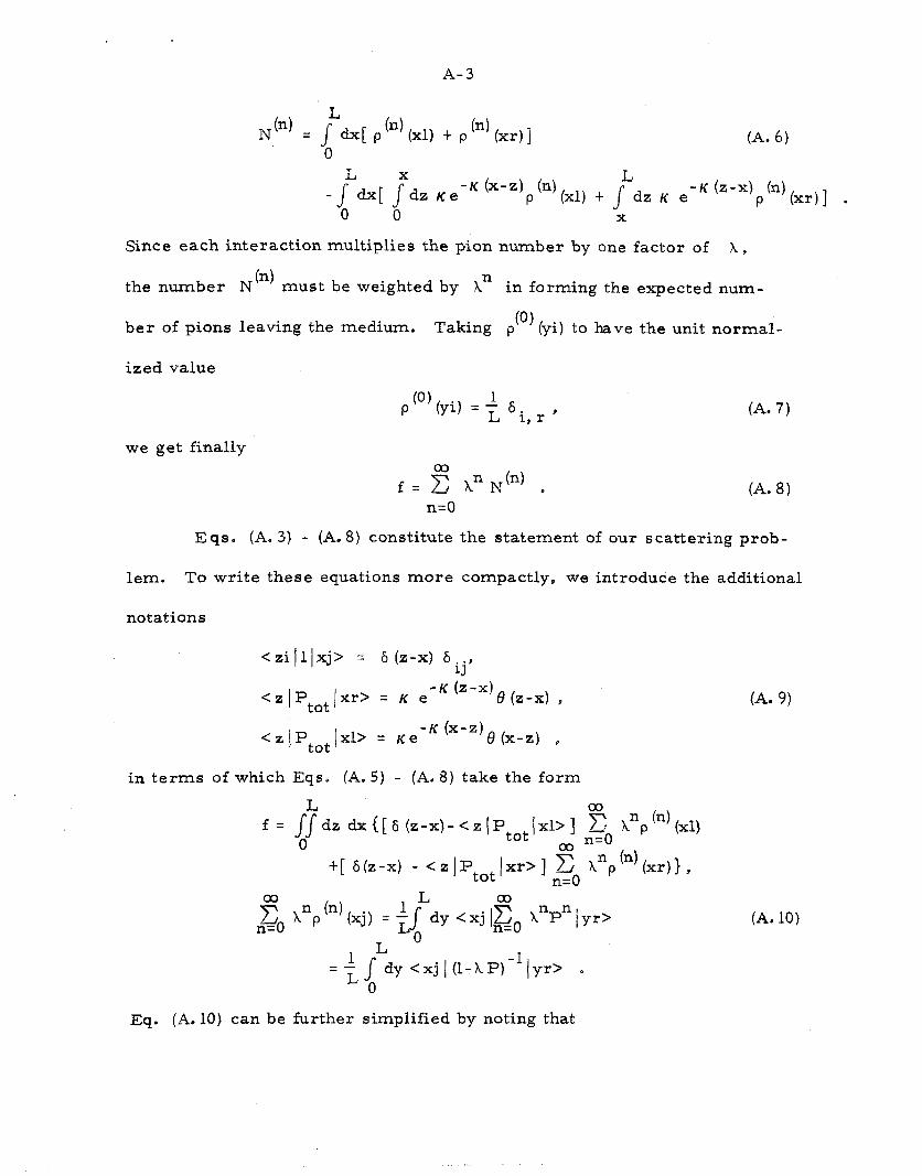
N(~) = fdx[ p (n) (xl) t p (n) (xr)] 0

(A. 6)

X

-? u

L dx.

dz K e-K (=dp (4

0 0 (xl) t s dz K e-K (z-x)p(n)(xr)] .

X

Since each interaction multiplies the pion number by one factor of X p

the number N b-4 must be weighted by Xn in forming the expected num-

ber of pions leaving the medium. Taking p (0) (yi) to have the unit normal-

ized value

p (0) fyi) =i6i

, r, (A. 7)

we get finally

f = 5 An J#) D (A. 8) n=O

Eqs. (A. 3) - (A. 8) constitute the statement of our scattering prob-

lem. To write these equations more compactly, we introduce the additional

notations

CziIlIxj> = 6 (z-x) b.., 13

< z I Ptot I xr> = K e -K (z-x)e (z-x) 9

< z I ptot I xl> = /ce -K (x-z)(g (x-z) ,

in terms of which Eqs, (A. 5) - (A. 8) take the form

f = Jydz dx([6 (z-x)-<z(~~~~/xl>] E pp (4 (XV 0 o. n=O

+[ h(z-x) - <z JPtot/xr> ] Z X n=O

n (n) (XT) } , p

Xnp (n) (xj) = -tiLdy < xj Igo XnPn 1 yr>

1 L 0

=- s dy <xj 1 (1-XP)-‘(yr> 0 LO

(A. 9)

(A. 10)

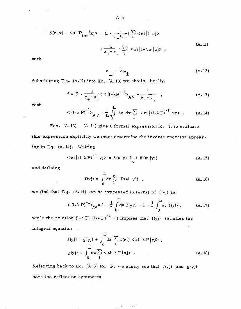
Eq. (A. 10) can be further simplified by noting that

A-4

S(Z-x) - <zlPtot/xj> = (1 - *) y <zi JlJxj> + -

t 1 22 Ut+U j, Czifl-hPIxj> I

(A. 11)

with

= xp a+ i Substituting E q. (A. 11) into Eq. (A. lo) we o’btain, finally,

(A. 12)

with

f= (l-rr ;, )< (l-xP)-l>Av + ~ : ~ , (A. 13) t - t -

< (l-AP)-l>*V = -1 L

JJ dz dy 23 <ziI (1-XP)-l(yr> . LO

(A. 14) i

Eqs. (A. 12) - (A. 14) g’ Ive a formal expression for f; to evaluate

this expression explicitly we must determine the inverse operator appear-

ing in Eq. (A. 14). Writing

czi 1 (l-Ap)-i (Yj> = 6(z-y) 6ij+ F(zi (yj) (A. 15)

and defining L

f(yj) = s dz x F(zi)yj) p 0 i

(A. 16)

we find that Eq. (A. 14) can be expressed in terms of f (yj) as

L c (l-xP)-l>AV= 1 t i J

L dy f(yl) , (A. 17)

0 dy f(yr) = 1 t i s

0

while the relation (1-XP) (1-XP)-l = 1 implies that f(yj) satisfies the

integral equation T

f(yj) = g(yj) t s dz r f(zi) < zi ) X P (yj> , 0 i

g(yj) = $ dzZ)<ziIkPlyj> . 0 i

(A. 18)

Referring back to Eq. (A. 3) for P, we easily see that f(yj) and g(yj)

have the reflection symmetry

A-5

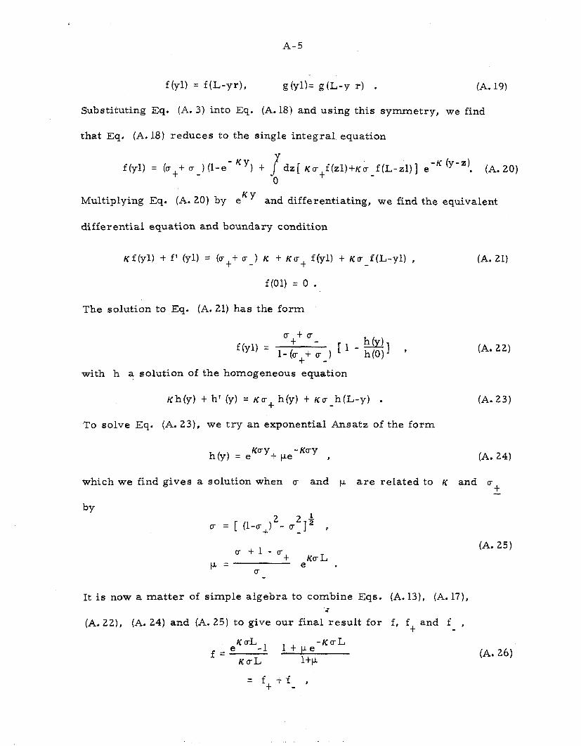
f(yl) = fb-yr), g (yl)= g&-y r) o (A. 19)

Substituting Eq. (A. 3) into Eq. (A. 18) and using this symmetry, we find

that Eq. (A. 18) reduces to the single integral equation

f(y1) = (ut-t u ) (l-e- KY) + P dz[ Krrtf(zl)tKr-f(L-zl)] e -K (y-z! (A. 20) 0

Multiplying Eq. (A. 20) by eK ’ and differentiating, we find the equivalent

differential equation and boundary condition

K ffyl) -t f’ (yl) = (ut+u ) K tKu + f(Yl) i- Ku fb-yl) , (A. 21)

f(01) = 0 l

The solution to Eq. (A. 21) has the form

f(yl) = utt u

I- (utt o- )

with h a solution of the homogeneous equation

(A. 22)

Kh(y) + h’ (y, = Ku+ My) + Ku h(L-y) . (A. 23)

To solve Eq. (A. 23), we try an exponential Ansatz of the form

h(y) = eKuYt pe-KuY P [A. 24)

which we find gives a solution when u and p are related to K and u t

bY

u = [ (l-uJ2- u ] 2*

p

u t1-cr t tJ,= u

eKFL .

It is now a matter of simple algebra to combine Eqs. (A. 13), (A. 17), f

(A. 22), (A. 24) and (A. 25) to give our final result for f, f and f t -’

f ie KuLml 1 + e-KuL

KuL 1W

(A. 25)

(A. 26)

= ft t ,f ,

A-6

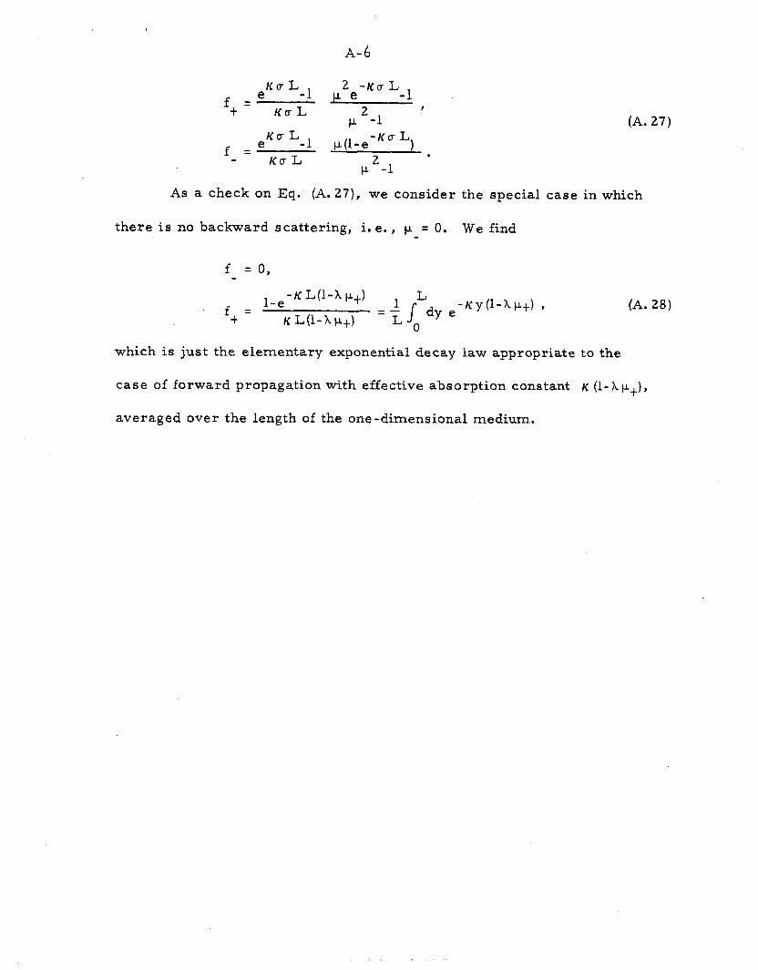
(A. 27) f+ =

eKUL -1 I-1

ze-Kcr Lsl

KUL 2 ,

f = eKu L-1 ,(l’.ezT L)

KaL P2-l *

As a check on Eq. (A. 27), we consider the special case in which

there is no backward scattering, i. e., = 0. We find

1 e-K L(l-A P+) f+= -

K L(l-h t-q)

1 L =- s

LO

dy e-Ky(l-b+) t (A. 28)

which is just the elementary exponential decay law appropriate to the

case of forward propagation with effective absorption constant K (l-Xv+),

averaged over the length of the one-dimensional medium.

B-l

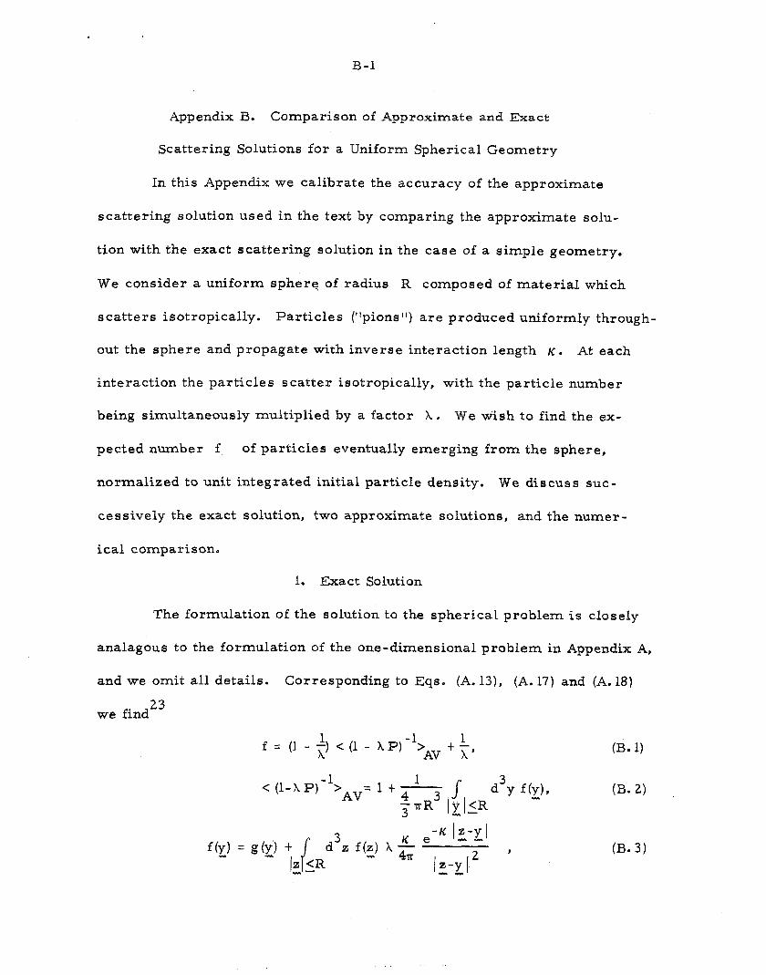
Appendix B. Comparison of Approximate and Exact

Scattering Solutions for a Uniform Spherical Geometry

In this Appendix we calibrate the accuracy of the approximate

scattering solution used in the text by comparing the approximate solu-

tion with the exact scattering solution in the case of a simple geometry.

We consider a uniform sphere of radius R composed of material which

scatters isotropically. Particles (“pions”) are produced uniformly through-

out the sphere and propagate with inverse interaction length K. At each

interaction the particles scatter isotropically, with the particle number

being simultaneously multiplied by a factor A. We wish to find the ex-

petted number f of particles eventually emerging from the sphere,

normalized to unit integrated initial particle density. We discuss suc-

cessively the exact solution, two approximate solutions, and the numer -

ical comparison.

1. Exact Solution

The formulation of the solution to the spherical problem is closely

analagous to the formulation of the one-dimensional problem in Appendix A,

and we omit all details. Corresponding to Eqs. (A. 13), (A. 17) and (A. 18)

we find 23

f = (l- +) < (1 - AP)% 1 AV +?

1 < (1-X P)-l>AV= 1 + - s

$R3 IpilR d3y f(x)?

(B. 1) (B-2)

(B. 3)

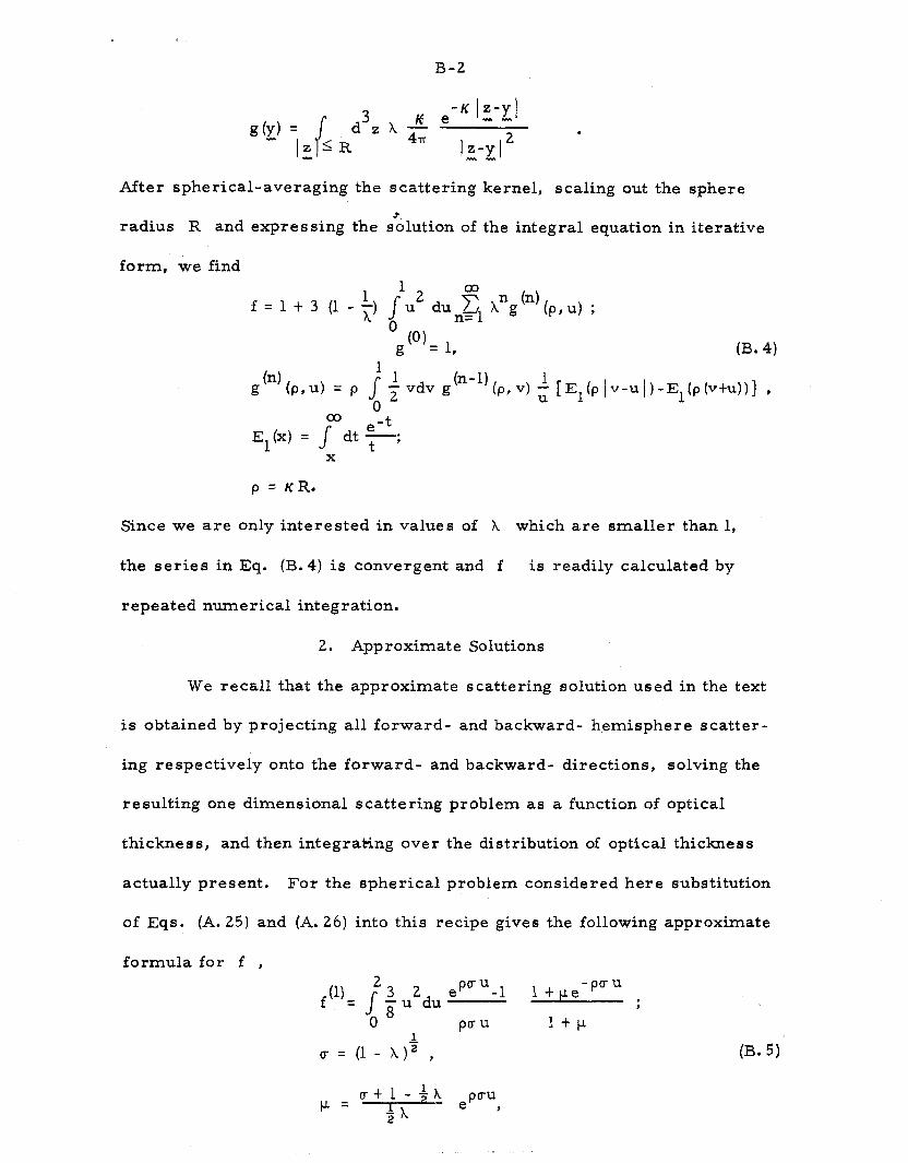
B-2

.

After spherical-averaging the scattering

radius R and expressing the s:lution of

kernel, scaling out the sphere

the integral equation in iterative

form, we find

f = 1 t 3 (l- $ Jlu2 O3 n (n) dung A g (p,u) ;

Og@) 1 = , 03.4)

gtn) (p, u) = p i i vdv g(n-l)(p, v) i [EI(P)v-uj)-E1(P(v+u))] 9

-t El(x) = Jmdt b;

X

P = KR.

Since we are only interested in values of A which are smaller than 1,

the series in Eq. (B.4) is convergent and f is readily calculated by

repeated numerical integration.

2. Approximate Solutions

We recall that the approximate scattering solution used in the text

is obtained by projecting all forward- and backward- h,emisphere scatter-

ing respectively onto the forward- and backward- directions, solving the

resulting one dimensional scattering problem as a function of optical

thickness, and then integrating over the distribution of optical thickness

actually

of Eqs,

formula

present. For the spherical problem considered here substitution

(A. 25) and (A. 26) into this recipe gives the following approximate

for f ,

f(l), 22u2du ePuU-1 1 t pemPuU , s O8

, PO-U l-tP

1 IT’= (1-A)‘) (B. 5)

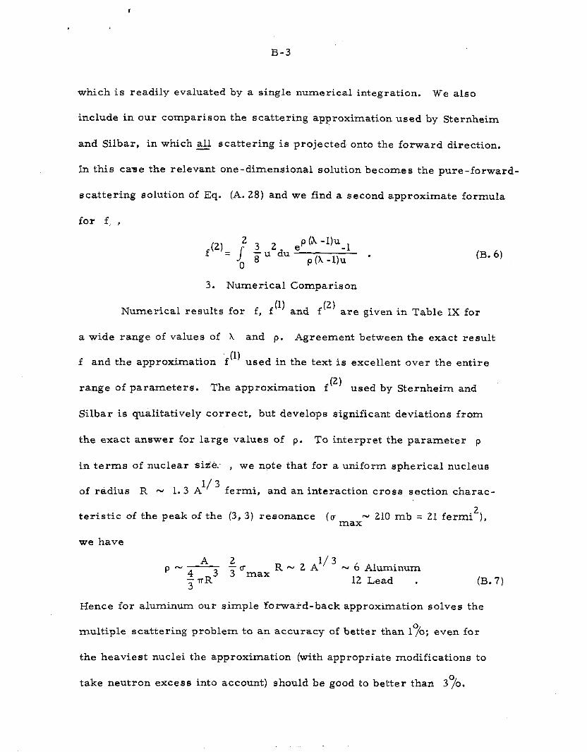
B-3

which is readily evaluated by a single numerical integration. We also

include in our comparison the scattering approximation used by Sternheim

and Silbar, in which all scattering is projected onto the forward direction. -

In this case the relevant one-dimensional solution becomes the pure-forward-

scattering solution of Eq. (A. 28) and we find a second approximate formula

for f; ,

f(2), 23 2 s -u du .P b -w-l

0 8 p(A-1)u ’

3. Numerical Comparison

Numerical results for f, f (1) and ft2) are given in Table IX

a wide range of values of X and p. Agreement between the exact

(B. 6)

for

result

f and the approximation f 0) used in the text is excellent over the entire

range of parameters. The approximation f (2) used by Sternheim and

Silbar is qualitatively correct, but develops significant deviations from

the exact answer for large values of p. To interpret the parameter p

in terms of nuclear siti& , we note that for a uniform spherical nucleus

of radius R N 1.3 A l/3 fermi, and an interaction cross section charac-

teristic of the peak of the (3,3) resonance (u max

N 210 mb = 21 fermi2),

we have

A 2 p-7

-rR3 -cr 3 RN 2 Ali w 6 Aluminum max

3 12 Lead a (B. 7)

Hence for aluminum our simple Forward-back approximation solves the

multiple scattering problem to an accuracy of better than lo/o; even for

the heaviest nuclei the approximation (with appropriate modifications to

take neutron excess into account) should be good to better than 30/o.

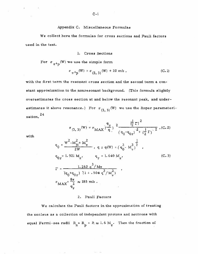
C-l

Appendix C , Miscellaneous Formulas

We collect here the formulas for cross sections and Pauli factors

used in the text.

1. Cross Sections

For o- Ttp(w) we use the simple form

~rr+pW) = ut3 ,)(W) + 20 mb p I, (C- 1)

with the first term the resonant cross section and the second term a con-

stant approximation to the nonresonant background. (This formula slightly

overestimates the cross section at and below the resonant peak, and under-

estimates it above resonance.) For (r (3, 3) (w)

we use the Roper parameteri-

zation, 24

with

W2-M;+ M2 1

90 = IT 2w ’ qzq(W)=($M;)2 ,

qor= 1.921 M , 7T

qr = 1.640 M1,,

3 I?= 1.262 q /MT

-(qOtqOr) 71 t .504 q2/+ ’

=MAX =% w185mb.

‘r

2. Pauli Factors

We calculate the Pauli factors in the approximation of treating

the nucleus as a collection of independent protons and neutrons with

equal Fermi- sea radii R n= Rp = R M 1.6 MTI. Then the fraction of

(C. 3)

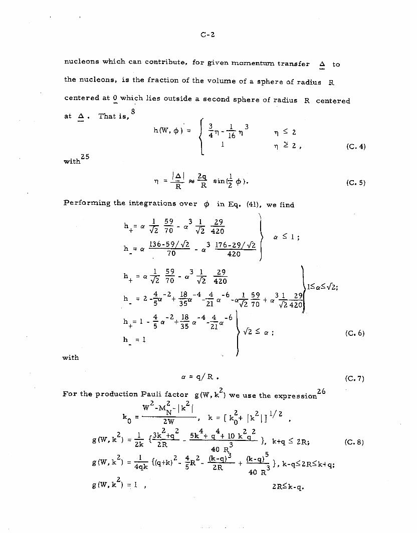
c-2

nucleons which can contribute, for given momentum transfer A to

the nucleons, is the fraction of the volume of a sphere of radius R

centered at 0 which lies outside a second sphere of radius R centered

at A. That is, 8

h(W, Q, 1‘ = $l-+T 3

112

1 122,

with”

q = IAl $9 - R

R sin+ #).

(C. 4)

(C. 5)

Performing the integrations over $ in Eq. (41), we find

h+= a ‘z $ _ o3 7

= Q 136-59/&Z i

CLl;

h 70

_ (y3 176;;09/J2

ht

h

with

ht= 1 - f Ly-2+s ,-4+-6 J2 5 CY ;

h =1 Cc. 6)

a!=q/R. (C. 7)

For the production Pauli factor g(W, k2) we use the expression 26

k. = W2-M;- 1 k2 1

2w , k= [k;+ jk21]1/2 ,

1, k+q s 2R; (C. 8)

gW,k2) = +jg {(a+k) 2 4 2 - ?R

- -kd- @d 2R

+

40 R3 } f k-q-<2R<k+ q:

gP+Wz) =1 , 2Rlk-q.

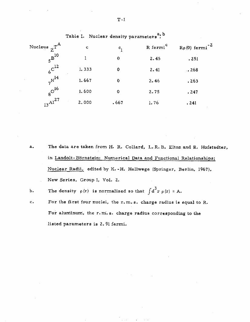
T-l

a, b Table I. Nuclear density parameters .

Nucleus zT A

C c1 R fermiC

sB 10

1 0 2.45

6’ 12

1.333 0 2.41

iN 14

1.667 0 ‘2.46

8O 16

1.600 0 2.75

13A1 27

2.000 . 667 1. 76

Rp (0) fermi -2

.251

. . 268

. 263

. 247

. 241

a.

b.

C.

The data are taken from H. R. Collard, L. R. B. Elton and R. Hofstadter,

in Landolt- Bornstein: Numerical Data and Functional Relationships;

Nuclear Radii, edited by IS. -H. Hellwege (Springer, Berlin, 1967),

New Series, Group I, Vol. 2.

The density p(r) is normalized so that Jd3r p(r) = A.

For the first four nuclei, the r. m. s. charge radius is equal to R.

For aluminum, the r. x-xi. s. charge radius corresponding to the

listed parameters is 2. 91 fermi.

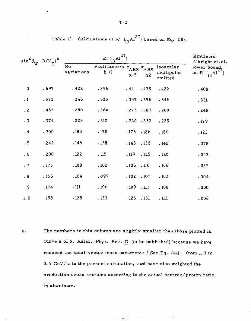
T-2

Table II. Calculations of R’ (13A127) based on Eq. (15).

sin2 6w a R’ (,,A~~71 Simulated

R (NT) Albright et. al. No Pauli factors uABS uABS Isoscalar lower bou variations h-l 97

X.5 X2 multipoles on R’ (,,A1 )

0

.l

. 697

. 573

. 465

. 374

. 300

. 242

. 200

. 175

. 166

. 174

. 198

. 422

. 346

. 280

. 225

. 180

. 146

. 122

. 108

.104

. 396

. 325

. 264

. 212

. 170

. 138

. 115

.102

. 411 .435

. 337 .356

. 273 -289

. 220 .232

l 176 .l86

.143 .150

. 119 . 125

.106 .110

l 102 .107

. lo9 .113

. 126 .131

omitted

.422 l 408

. 321

,245 . 2

. 3

.4

.5

46

.7

.8

. 9

1. 0

a.

. 111

,128

. 099

.l06

. 123

. 346

. 280

. 225

. 180

. 145

.12Q

. 106

. 102

.lO8

. 125

. 179

.123

.078

. 043

. 019

. 004

,000

. 006

The numbers in this column are slightly smaller than those plotted in

curve a of S. Adler, Phys. Rev. g (to be published) because we have

reduced the axial-vector mass parameter [ See Eq. (44)] from 1.0 to

0. 9 GeV/ c in the present calculation, and have also weighted the

production cross sections according to the actual neutron/proton ratio

in aluminum.

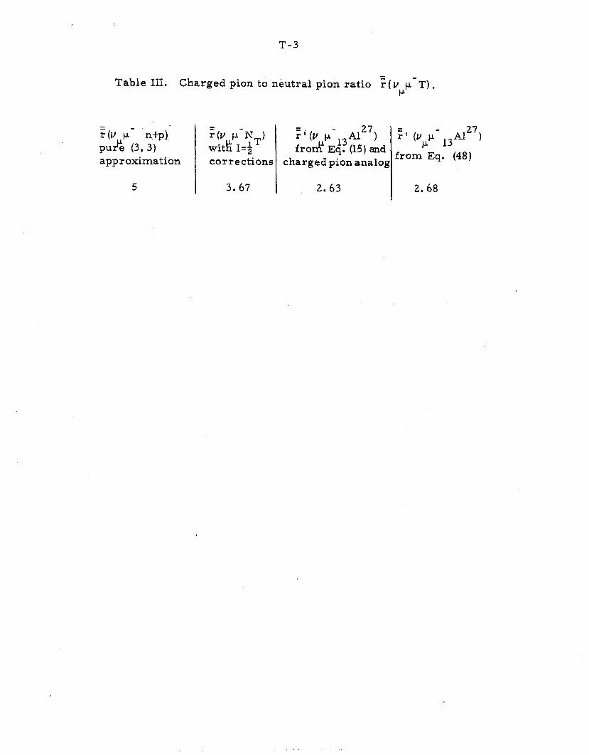
T-3

Table III. Charged pion to neutral pion ratio F ( vPp- T) .

FCV p- n.+p). pul)Le (3, 3) approximation

:(v p-N ) =: wit& I=iT

2-l (v I+- A127) fxdf & (15) and

:I (v p- lsA127)

corrections charged pion analog frompEq . (48)

5 3.67 2.63 2.68

T-4

Table IV. Simulated 2 (13Al 272 - ;k ) and A(13A1 27 2 ;k ) obtained

from electroproduction and charge exchange correction models.

k2 (GeV/ c)’

0

. 1

. 2

.3

.4

. 6

.8

1. 0

1. 4

1.8

ki= 2 GeV/c kl:= 6 GeV/c

A(13M 27;k2) d(13A127;k2) A(,3JJ27;k2) dt13A1 27;k2)

. 191

. 181

.169

l 606

. 688

. 702

. 702

. 698

. 694

.690

. 690

. 688

. 686

e 188

s 179

e 167

a 162

o 158

. 608

. 682

.694

. 164

. 160

. 157

. 156

. 155

. 155

. 156

. 154

.152

0 150

. 147

D 145

e 694

. 690

. 684

. 680

.676

a 672

e 666

T-5

Table V. Test of first averaging approximation for R’ (13A127).

R’ (13A127)

sin’ 0 w

0

. 1

. 2

. 3

. 4

. 5

. 6

. 7

.8

. 9

1. 0

From Eq. (23.)

. 433

. 355

. 288

. 232

. 186

e 151

. 127

. 113

. 109

. 116

. 134

From Eq. (15)

,422

. 346

. 280

. 225

. 180

. 146

. 122

. 108

l 104

D 111

.128

T-6

Table VI. Test of second averaging approximation for R’ (13A127)m

R’ (13AlL ’ )

2 sin 8

-Iv

0

.l

. 2

. 3

.4

.5

. 6

. 7

.8

. 9

1.0

.692

.697

l 707

.727

. 763

. 820

.903

LO1

1.12

1.19

1. 22

: (zy”-NT)

3.67

3.67

3.67

3.67

3.67

3.67

3.67

3.67

3.67

3.67

3.67

From Eq. (24) From Eq. (15)

.432 .422

. 356

. 289

. 234

. 189

. 154

. 129

. 116

. 112

l 119

0 346

0 280

a 225

.180

. 136

. 146

. 122

. 108

. 104

e 111

a 128

T-7

Table VII. Averaged charge exchange parameters for various nuclei.

Nucleus - z a ;i

gB 10

. 846 .0363 .125

6’ 12

.811 -0450 .138

7N 14

. 790 .0498 .144

8’ 16 .807 .0460 ,139

13*l 27

. 724 .0642 ,162

T-8

Table VIII. Effect of modificationsuE the model on 3 (13A127) ,

iJ(,,A127)

No variations Nucleon motion Pauli factors included h-l uABS uABS

x.5 x2

. 162 . 142 .187 . 175 ,145

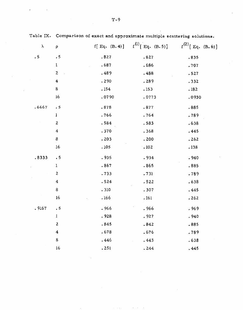
Table IX.

A

.5

. 6667

. 8333

. 9167

T-9

Comparison of exact and approximate multiple scattering solutions.

P f[ Eq. CB. 4) 1 ,Q)[ Eq (B 5)3 . 0 ft2)[ Eq (B 6)] l .

.5 . 827

1 .687

2 .489

4 . 290

8 . 154

16 . 07 90

. 5

1

2

4

8

16

. 5 . 935

1 . 867

2 l 733

4 . 524

8 . 310

16 . 166

. 5

1

2

4

8

16

.878

. 766

. 584

. 370

. 203

. 105

. 966 . 966

. 928 . 927

. 845 ,842

l 678 . 676

.446 .443

. 251 .244

. 827

. 686

.488

. 289

. 153

.0773

. 877

. 764

. 583

. 368

. 200

. 102

.934

. 865

. 731

. 522

. 307

4 161

. 835

. 707

. 527

. 332

. 182

. 0930

. 885

. 789

. 638

.445

. 262

. 138

.940

.885

. 789

. 638

. 445

. 262

. 969

.940

.885

l 789

. 638

,445

1.

2.

3.

4.

5.

6.

7.

R-l

References

B. W. Lee, Phys. Letters 4OB 420 (1972); W. Lee, Phys. Letters

40B, 423 (1972).

D. H. Perkins, Neutrino Interactions , in Proceedings of the XVI

International Conference on High Energy Physics, Chicago-Batavia,

September, 1972, Vol. 4, p. 189.

M. M. Sternheim and R, R. Silbar, Phys. Rev. D6 3117 (1972). -’

Earlier studies of pion charge exchange in nuclei involved the use

of Monte Carlo techniques rather than analytical models. See N.

Metropolis et. al., Phys. Rev. 110, 204 (1958); Yu. A. Batusov

et. al. , J. Yad. Fiz. 6, 158-164 (1967) [ English translation: Soviet

Journal of Nuclear Physics 6, 116 (1968)] ; C. Franzinetti and C.

Manfredotti, CERN report NPA/ Int 67 - 30 (unpublished); C.

Manfredotti, CERN report NPA/Int 68-8 (unpublished).

E. Fermi, Ricerca Sci. z (2), 13 (1936) and AECD-2664 (1951). For

a discussion see E. Amaldi, The Production and Slowing Down of

of Neutrons, in S. Fltigge, ed., Handbuch der Physik, V. 38, No. 2

(Springer, Berlin, 1959) and G. M. Wing, Ref. 20.

S. L. Adler, Ann. Phys. 50, 189 (1968) and Phys. Rev.D(to be -

published).

We adhere to the notations of Ref. 5 wherever possible.

A detailed numerical calculation of the effect of Fermi motion on the

production cross sections indicates a substantial broadening of the

resonance and a simultaneous shift of the resonance center to lower

excitation ene rgie 6. Both effects increase with increasing kze The

effective upper edge of the resonance, however, is not shifted and

so an integration over experimental data from the effective thresh-

old (which differs greatly from the threshold for pion production on

nucleons at rest) to a fixed upper cutiff of

&,L)MAx’ (1.47 GeV)‘-MN+ /k2 1

includes virtually the entire resonance. 2MN

The area under the reson-

ance obtained this way is essentially the same as the area obtained

8.

9.

10.

11.

12.

13.

14.

15.

16.

17.

18.

,R-2

when Fermi motion is neglected. Hence we expect production Fermi

motion effects to be relatively unimportant once the excitation energy

has been integrated out, provided, of course, that one is not too closeto

a kinematic threshold for (3, 3) -resonance production.

S. M. Berman, in Proceedings of the International Conference on

Theoretical Physics of Very High Energy Phenomena, CERN (1961).

This restriction is of course not necessary in principle. The exten-

sion of our multiple scattering model to take a neutron excess into

account will be given elsewhere (S. L. Adler, to be published).

Since Eq. (15) involves an integration over excitation energy k L 0’

we expect the Fermi motion smearing of the production cross sec-

tion to be relatively unimportant, and neglect it in the applications

of Eq. (15) in Section 3.

The dominant resonant vector and axial-vector multipoles lead to

different angular dependences of the production cross section.

Some acceptance dependence in x could be tolerated, since it would

tend to cancel between the numerator and denominator of R’ .

We are indebted to A. Kerman for a discussion about this point.

When Pauli effects are included, the forward peak is washed out,

but the backward peak remains.

S. Weinberg, Phys. Rev. Letters 19, 1264 (1967); Phys. Rev. Letters -

27 1688 (1971); A. Salam, Elementary Particle Theory, edited by -’

N. Svartholm (Almquist Forlay, Stockholm, 1968), p. 367; G.

’ t Hooft, Nuclear Physics B35, 167 (1971).

This is strictly true only when NT =Z(ptn), whereas in the production

calculation we have used NT= 13p t 14n. The numerical effect of

this change is small.

C. H. Albright, B. W. Lee, E. A. Paschos and L. Wolfenstein, Phys.

Rev. D7, 2220 (1973). Here G, BC and - CY denote, respectively, the

structure constant.

effect of taking account of

Fermi constant, Cabibbo angle and fine

The ratio 3.67 also includes the (small)

the actual n/p ratio in aluminum.

R-3

19. The corresponding prediction for incident antineutrinos is 2. 32.

20. S. L. Adler, Ann. Phys. 50, 189 (1968), Eq. (4E.7). -

21. Qualitatively, both nucleon Fermi motion and the deviations of

the scattering angular distribution from pure “forward-back”

would be expected to produce an angular, smearing of the result

of Eq. (51).

22. For a nice pedagogical discussion of one-dimensional multiple ,

scatte’ring, see G. M. Wing, An Introduction to Transport Theory

(Wiley, New York, 1962).

23. The methods leading to these equations are discussed in K. M.

Case and P. F. Zweifel, Linear Transport Theory(Addison-Wesley,

Reading, Mass. , 1967). See especially Section 3.6.

24. L. D. Roper, Phys. Rev. Letters 12, 340 (1960). -

25. We have approximated A by the isobar frame momentum transfer.

The approximation is bad only when q is so large that h = 1.

26. Eq. (C. 8) is obtained from Eq. (6~. 6) of Ref. 18.