Named Entity Recognition:

A Literature Survey

Rahul Sharnagat

11305R013

June 30, 2014

In this report, we explore various methods that are applied to solve NER. In section 1, we introduce

the named entity problem. In section 2, various named entity recognition methods are discussed in three

three broad categories of machine learning paradigm and explore few learning techniques in them. In

the first part, we discuss various supervised techniques. Subsequently we move to semi-supervised and

unsupervised techniques. In the end we discuss about the method from deep learning to solve NER.

1 Introduction

Named Entity Recognition(NER) is one of the major task in Natural Language Processing(NLP). NER

is an active area of research for past twenty years. A lot of progress has been made in detecting named

entities but NER still remains a big problem at large.

The main focus of this work is improving the NER system for Indian Languages using supervised

and unsupervised methods. We explore various statistical measure for identifying Named Entities, study

the deep learning/Neural Network approaches for Named entity recognition. In this chapter we give an

introduction to the Named Entity Recognition task, its application and motivation for pursuing research

in this area.

1.1 What is Named Entity?

In data mining, a named entity is a word or a phrase that clearly identifies one item from a set of other

items that have similar attributes. In the expression named entity, the word named restricts the scope

of entities that have one or many rigid designators that stands for a referent. Usually, Rigid designators

include proper names, but it depends on domain of interest that may refer the reference word for object

in domain as named entities. For example, in molecular biology and bio-informatics, entities of interest

are genes and gene products.

1

1.2 Named Entity Recognition Task

Named Entity Recognition(NER) is the process of locating a word or a phrase that references a particular

entity within a text. The NER task first appeared in the Sixth Message Understanding Conference (MUC-

6) Sundheim (1995) and involved recognition of entity names (people and organizations), place names,

temporal expressions and numerical expressions.

In MUC-6, Named entities(NEs) were categorized into three types of label, each of which uses specific

attribute for a particular entity type. Entities and their labels were defined as follows:

• ENAMEX: person, organization, location

• TIMEX: date, time

• NUMEX: money, percentage, quantity

Example of annotation from MUC-7 data in English:

The <ENAMEX TYPE="LOCATION">U.K</ENAMEX> satellite television broadcast-

er said its subscribers base grew <NUMEX TYPE="PERCENT">17.5 percent</N-

UMEX> during <TIMEX TYPE="DATE"> the past year</TIMEX> to 5.35 million

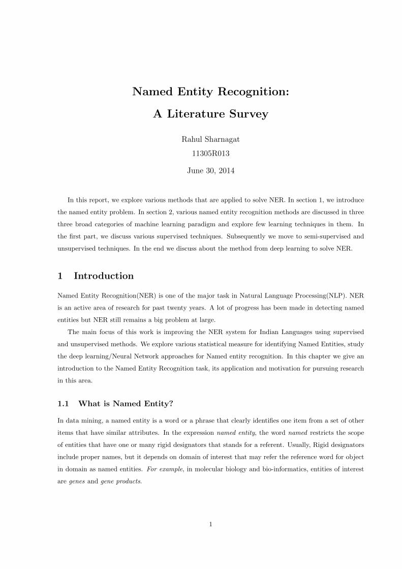
Different fine grained or domain dependent annotation schemes have been proposed by many re-

searchers. Consider a example from Lee et al. (2006) in figure 1. Lee et al. (2006) divided the classification

of named entities into nine broad classes like person, organization, location, product, art, event, building

etc. These classes have been further fine grained into sub categories. In practice, it is convinient to work

with coarse classification than fine grain classification due to data sparsity.

2 Approaches to NER

In this section, we will look into some of the methods to NER.

2.1 Supervised methods

Supervised methods are class of algorithm that learn a model by looking at annotated training examples.

Among the supervised learning algorithms for NER, considerable work has been done using Hidden

Markov Model (HMM), Decision Trees, Maximum Entropy Models (ME), Support Vector Machines

(SVM) and Conditional Random Fields(CRF). Typically, supervised methods either learn disambiguation

rules based on discriminative features or try to learn the parameter of assumed distribution that maximizes

the likelihood of training data. We will study each of these methods in detail in next sections.

2.1.1 Hidden Markov Models

HMM is the earliest model applied for solving NER problem by Bikel et al. (1999) for English. Bikel

introduced a system, IdentiFinder, to detect NER.

2

Figure 1: Fined grained entity tagset

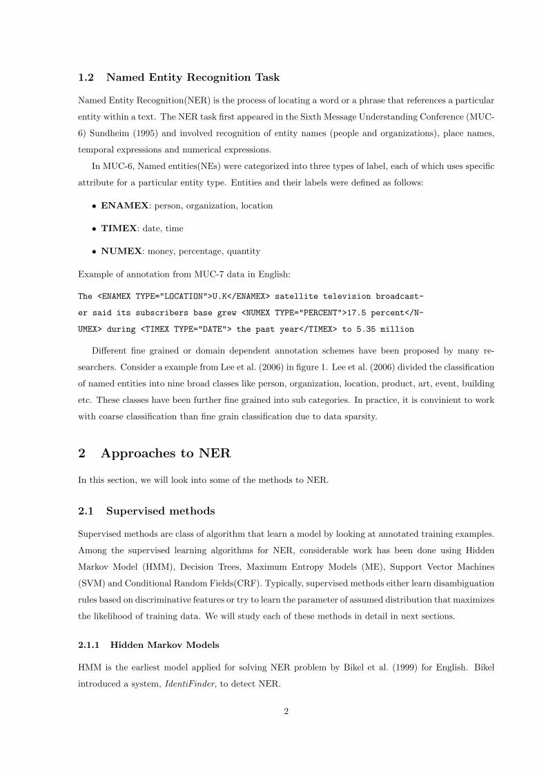
According to Bikel’s formulation of the problem in the Identifinder system, only a single label can be

assigned to a word in context. Therefore, the model assigns to every word, either one of the desired classes

or the label NOT-A-NAME to represent ”none of the desired classes”. State diagram for his model is

shown in Figure-2 For tagging a sentence, the task is to find the most likely sequence of name-classes(NC)

given a sequence of words(W):

maxPr(NC|W )

HMM is a generative model, i.e. it tries to generate the data, sequences of words W, and labels NC from

distribution parameters.

Pr(NC|W ) =Pr(W,NC)

Pr(W )

The Viterbi algorithm Forney (1973) is used to maximize Pr(W,NC) through the entire space of all

possible name-class assignments. Bikel modeled the generation in three steps:

• Select a name-class nc, conditioned on the previous name-class and previous word.

• Generate the first word inside the name-class, conditioning on the current and previous name-

3

Person

Organization

Not-a-name

START-OF-SENTENCE END-OF-SENTENCE

(five other name classes)

Figure 2: State Diagram for Identifier

classes.

Pr(nc|nc−1, w−1).P r(< w, f >first |nc, nc−1)

• Generate all subsequent words inside the current name-class, where each subsequent word is con-

ditioned on its immediate predecessor

Pr(< w, f > | < w, f >−1, nc)

There is also a distinct end marker ”+end+”, so that the probability may be computed for any current

word to be final word of its name-class

Pr(< +end+, other > | < w, f >final, nc)

Consider an example :

Mr. Jones eats.

Correct annotation for such a sentence is:

Mr. <ENAMEX TYPE=”PERSON”>Jones</ENAMEX> eats.

Then a max likelihood equation from the search space would be:

Pr(NOT-A-NAME | START-OF-SENTENCE, +end+) * Pr(\Mr." | NOT-A-NAME, START

-OF-SENTENCE) * Pr(+end+ | "Mr.", NOT-A-NAME) * Pr(PERSON | NOT-A-NAME ,

"Mr.") * Pr("Jones" | PERSON, NOT-A-NAME) * Pr(+end+ | "Jones" PERSON) *

Pr(NOT-A-NAME | PERSON, "Jones") * Pr("eats" | NOT-A-NAME, PERSON) * Pr(

"." | \eats", NOT-A-NAME) * Pr(+end+ | ".", NOT-A-NAME)* Pr(END-OF-SENTE-

NCE | NOT-A-NAME ".")

4

IdentiFinder reported NE accuracy of 94.9% and 90% for a mixed case English (MUC-6 data and a

collection of Wall Street Journal documents) and mixed case Spanish (MET-1 data, comprised of articles

from news agencies AFP) respectively.

Zhou and Su (2002) modified the IdentiFinder model by using mutual information. Given a token

sequence Gn1 = g1 g2 g3 · · · gn, the goal of the learning algorithm is to find a stochastically optimal tag

sequence Tn1 = t1 t2 t3 · · · tn that maximizes

Pr(Tn1 |Gn1 ) = logPr(Tn1 ) + logPr(Tn1 , G

n1 )

Pr(Tn1 ) Pr(Gn1 )

Unlike IdentiFinder, Zhou’s model directly generates original NE tags from the output words of the

noisy channel. Zhou’s model assumes mutual information independence while HMM assumes conditional

probability independence.

The HMM-based chunk tagger gave an accuracy of 96.6% on MUC-6 data and 94.1% on MUC-7 data.

2.1.2 Maximum Entropy based Model

Maximum entropy model, unlike HMM, are discriminative model. Given a set of features and training

data, the model directly learns the weight for discriminative features for classification. In Maximum

entropy models, objective is to maximize the entropy of the data, so as to generalize as much as possible

for the training data. In ME models each feature is associated with parameter λi. Conditional probability

is thus obtained as follows:

P (f |h) =

∏i λ

gi(h,f)i

Zλ(h)

Zλ(h) =∑f

∏i

λgi(h,f)i

Maximizing the entropy ensures that for every feature gi, the expected value of gi, according to M.E.

model will be equal to empirical expectation of gi in the training corpus.

Finally, Viterbi algorithm is used to find the highest probability path through the trellis of conditional

probabilities which produces the required valid tag sequences.

The MENE system

The MENE system from Borthwick (1999) uses an extraordinarily diverse set of knowledge sources

in making its tagging decisions, It makes use of broad array of gazetteers and dictionaries of single

or multi-word terms like first name, company name, corporate suffixes. It uses wide variety of

feature like binary features, lexical features, section features, external systems output, consistency

and reference resolution.

The 29 tags of MUC-7 form the space of futures for the maximum entropy formulation of NE

detection. A maximum entropy solution to this allows the computation of p(f |h) for any f from

the space of possible futures, F , for every h from the space of possible histories, H. A history of all

the conditional data that helps the maximum entropy model to make decisions about the possible

future.

5

Accuracy reported for the MENE system on MUC-7 data is 88.80%.

Curran’s ME Tagger

Curran and Clark (2003) applied the maximum entropy model to the named entity problem. They

used the softmax approach to formulate the probability P (y|x). The tagger uses the model of the

form :

P (y|x) =1

Z(x)exp(

n∑i=1

λifi(x, y))

where y is the tag, x is the context and fi(x, y) is the feature with associated weight λi.

Hence the overall probability for the complete sequence of y1 · · · yn and words sequence w1 · · ·wn is

approximated as:

P (y1 · · · yn|w1 · · ·wn) ≈n∏i=1

Pr(yi|xi)

where xi is a context vector for each word wi. The tagger uses beam search to find the most

probable sequence given the sentence.

Curran reported the accuracies of 84.89% for the English test data and 68.48% for the German test

data of CoNLL-2003 shared task.

2.1.3 SVM Based Models

Support Vector Machine was first introduced by Cortes and Vapnik (1995) based on the idea of learning

a linear hyperplane that separate the positive examples from negative example by large margin. Large

margin suggests that the distance between the hyperplane and the point from either instances is maximum.

The points closest to hyperplane on either side are known as support vectors.

Figure-3 shows the geometric interpretation. The linear classifier is based on two parameters, a weight

vector W perpendicular to the hyperplane that separates the instances and a bias b which determines the

offset of the hyperplane from the origin. A sample x is classified as positive instance if f(x) = wx+ b > 0

and negative otherwise. If the data points are not linearly separable, then a slack is used to accept some

error in classification. This prevents the classifier to overfit the data. When there are more than two

classes, a group of classifiers are used to classify the instance.

McNamee and Mayfield (2002) tackle the problem as binary decision problem,i.e. if the word belongs

to one of the 8 classes, i.e. B- Beginning, I- Inside tag for person, organization, location and misc tags.

Thus there are 8 classifiers trained for this purpose. All feature used were binary. 258 orthography and

punctuation features and 1000 language-related features were used. Window size was 7, that made the

number of features used to 8806.

To produce a single label for each token, the set S of possible tags were identified. If S was empty tag

O was assigned else most frequent tag was assigned. If both beginning and inside tags were present then

beginning tag was chosen.

For CoNLL 2002 data, reported accuracies were 60.97 and 59.52 for Spanish and Dutch respectively.

6

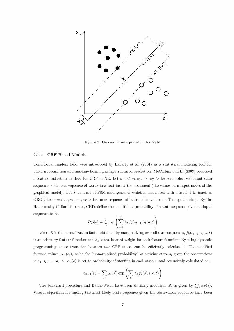
Figure 3: Geometric interpretation for SVM

2.1.4 CRF Based Models

Conditional random field were introduced by Lafferty et al. (2001) as a statistical modeling tool for

pattern recognition and machine learning using structured prediction. McCallum and Li (2003) proposed

a feature induction method for CRF in NE. Let o =< o1, o2, · · · , oT > be some observed input data

sequence, such as a sequence of words in a text inside the document (the values on n input nodes of the

graphical model). Let S be a set of FSM states,each of which is associated with a label, l L, (such as

ORG). Let s =< s1, s2, · · · , sT > be some sequence of states, (the values on T output nodes). By the

Hammersley Clifford theorem, CRFs define the conditional probability of a state sequence given an input

sequence to be

P (s|o) =1

Zexp

(T∑t=1

λkfk(st−1, st, o, t)

)where Z is the normalization factor obtained by marginalizing over all state sequences, fk(st−1, st, o, t)

is an arbitrary feature function and λk is the learned weight for each feature function. By using dynamic

programming, state transition between two CRF states can be efficiently calculated. The modified

forward values, αT (si), to be the ”unnormalized probability” of arriving state si given the observations

< o1, o2, · · · , oT >. α0(s) is set to probability of starting in each state s, and recursively calculated as :

αt+1(s) =∑s′

αt(s′) exp

(∑k

λkfk(s′, s, o, t)

)

The backward procedure and Baum-Welch have been similarly modified. Zo is given by∑s αT (s).

Viterbi algorithm for finding the most likely state sequence given the observation sequence have been

7

modified from its HMM form.

Experiments were performed on CoNLL 2003 shared task data, and achieved an accuracy of 84.04%

for English and 68.11% for German.

2.2 Semi-Supervised Methods

Semi supervised learning algorithms use both labeled and unlabeled corpus to create their own hypothesis.

Algorithms typically start with small amount of seed data set and create more hypothesis’ using large

amount of unlabeled corpus. In this section, we will have a look at some of the semi-supervised NER

system.

2.2.1 Bootstrapping based

Motivation for semi-supervised algorithm is to overcome the problem of lack of annotated corpus and

data sparsity problem. Semi-supervised usually starts with small amount of annotated corpus, large

amount of unannotated corpus and a small set initial hypothesis or classifiers. With each iteration, more

annotations are generated and stored until a certain threshold occurs to stop the iterations.

NER using AdaBoost Carreras et al. (2002) have modeled the Named entity identification task

as sequence labeling problem through BIO labeling scheme.Input is considered as word sequence

to label with one of the Beginning of NE (B-) tag, Inside of tag (I-) and outside of NE (O-) tag.

Three binary classifiers are used for tagging, one corresponding to each tag.

Orthographic and semantic features were evaluated over a shifting window allowing a relational

representation of examples via many simply binary propositional features.

The binary AdaBoost is used to with confidence rated predictions as learning algorithm for the

classifiers. The boosting algorithm combines several fixed-depth decision trees. Each tree is learned

sequentially by presenting the decision tree a weighting over the examples which depend on the

previous learned trees.

The Spanish data corresponds to the CoNLL 2002 Shared Task Spanish data and shows aperfor-

mance of 79.28%

2.3 Unsupervised Methods

A major problem with supervised setting is requirement of specifying large number of features. For

learning a good model, a robust set of features and large annotated corpus is needed. Many languages

don’t have large annotated corpus available at their disposal. To deal with lack of annotated text across

domains and languages, unsupervised techniques for NER have been proposed.

8

2.3.1 KNOWITALL

KNOWITALL is domain independent system proposed by Etzioni et al. (2005) that extracts information

from the web in an unsupervised, open-ended manner. KNOWITALL uses 8 domain independent

extraction patterns to generate candidate facts.

For example, the generic pattern ”NP1 such as NPLIST2” indicates that the head of each simple noun

phrase(NP) in the list of NPLIST2 is a member of class named NP1. It then automatically tests the

plausibility of the candidate facts it extracts using pointwise mutual information (PMI) computed using

large web text as corpus. Based on PMI score, KNOWITALL associates a probability with every facts

it extracts, enabling it to manage the trade-off between precision and recall. It relies on bootstrapping

technique that induces seeds from generic extraction patterns and automatically generated discriminator

phrases.

2.3.2 Unsupervised NER across Languages

Munro and Manning (2012) have proposed a system that generates seed candidates through local, cross-

language edit likelihood and then bootstraps to make broad predictions across two languages, optimizing

combined contextual, word-shape and alignment models. It is completely unsupervised, with no manually

labelled items, no external resources, only using parallel text that does not need to be easily alignable.

The results are strong, with F ¿ 0.85 for purely unsupervised named entity recognition across languages,

compared to just F = 0.35 on the same 37 data for supervised cross-domain named entity recognition

within a language. A combination of unsupervised and supervised methods increases the accuracy to F

= 0.88. The tests were done on the parallel corpus of English and Haitian Krreyol text messages used in

the 2010 Shared Task for the Workshop on Machine Translation.

A sample sentence from the data:

Kreyol: Lopital Sacre-Coeur ki nan vil Milot, 14 km nan sid vil Okap, pre pou li resevwa moun

malad e lap mande pou moun ki malad yo ale la.

English: Sacre-Coeur Hospital which located in this village Milot 14 km south of Oakp is ready

to receive those who are injured. Therefore, we are asking those who are sick to report to that

hospital.

3 Informative measures

3.1 Features

Feature engineering is a foremost essential task of NER for all classifiers. In this section, we describe

various features that have been used in existing NER systems. Features are descriptors or characteristic

attributes of words designed for algorithmic consumption. Features can be specified in numerous ways

9

using boolean values, numeric or nominal values. For example, a hypothetical NER system may be

represented using 3 attribute:

• A Boolean attribute with the value true if the first character of the word is capitalized and false

otherwise

• A numeric attribute corresponding to the length, in characters, of the word

• A nominal attribute corresponding to the lowercased version of the word

With above of set of features, the sentence ”The president of Apple eats an apple.” . This sentence

can be represented using following feature vectors:

<true,3,"the">,<false,9,"president">,<false,2,"of">,<true,5,"apple">,

<false,4,"eats">,<false,2,"an">,<false,5,"apple">

Usually, the NER problem is resolved by applying a rule system over the features. For instance,

a system might have two rules, a recognition rule: ”capitalized words are candidate entities” and

a classification rule:” the type of candidate entities of length greater than 3 words is organization”.

Specifying these helps to identifying the entities to certain extent. However, real systems tend to be

much more complex and their rules are often create or expanded by automatic learning algorithm. Next,

we describe the features that are most often used for the identification of named entities. We organize

the them in 2 categories: Word-level features and List lookup features.

3.1.1 Word level features

Word level features are related to the character level feature of words. They specifically describe word

case, punctuation, numerical value and special characters. Table ?? lists subcategories of word-level

features.

3.1.2 Digit pattern

Digits can express wide range of useful information such as dates, percentages, intervals, identifiers etc.

Certain patterns of digits gives strong signal about the type of named entities. For example, two digits

and four digit numbers can stand for years and when followed by an ”s”, they can stand for a decade.

Digits followed by units stands for quantity such as 10Kg.

3.1.3 Common word ending

Morphological features are essentially related to the words affixes and root word. Named entities also

has common suffixes features. For example, various city names have common suffix ”pur” like in Nagpur,

Raipur, Jaipur, Udaipur and so on. A system should learn that a human profession often ends in ”ist”

like in cyclist, journalist etc.

10

Features Examples Examples

Case Starts with a capital letter

Words is all uppercased

The word is mixed case (e.g., eBay, McDonald)

Punctuation Ends with period, has eternal period (e.g., Prof., B.B.C.)

Internal apotrophe, hyphen or ampersand (e.g. O’Reilly)

Digit Digit pattern

Cardinal and ordinal

Roman number

Word with digits

Character Possessive mark, first person pronoun

Greek letters

Morphology Prefix, suffix, singular version, stem

Common ending

Part-of-speech Proper name, verb, noun, foreign words

Function Alpha, non-alpha, n-gram

Lowercase, uppercase version

Pattern, summarized pattern

Token length, phrase length

Table 1: Word level features for NER

11

3.1.4 Functions over words

Features can be extracted by applying functions over words. An example a feature can be created by

applying a non alpha function over the word to create word level features like nonAlpha(I.B.M.) = ....

Another method is to use character n-grams as features.

3.1.5 Patterns and summarized patterns

Pattern feature is to map words onto a small set patterns over character types. For instance, a pattern

feature might map all uppercase letters to ”A”, all lower case letters to ”a”, all digits to ”0” and

punctuation to ”-”:

x=”I.B.M”: getPattern(x)=”A-A-A-”

x=”Model-123”: getPattern(x)=”Aaaaa-000”

The summarized pattern features is a condensed form of the above pattern feature in which consecutive

similar pattern types that are repeated are removed. For instance, for the preceding example:

x=”I.B.M”: getPattern(x)=”A-A-A-”

x=”Model-123”: getPattern(x)=”Aa-0”

3.1.6 List lookup features

Lists are the privileged feature in NER. The terms ”gazetteers”, ”lexicon” and ”dictionary” are used

interchangeably with the term ”list”. List feature signifies a is a relationship for the entities included in

the list. (e.g., Delhi is a city). If a word is included in the list, the probability of this word appearing in

a sentence to be named entity is high.

• General dictionary Common nouns listed in a dictionary are useful, for instance, in the disambigua-

tion of capitalized words in ambiguous position (e.g. sentence beginning). Mikheev et al. (1999)

reports that from 2677 words in ambiguous position in a given corpus, a general dictionary lookup

allows identifying 1841 common nouns out of 1851 (99.4%) while only discarding 171 named entities

out of 826 (20.7%). In other words, 20.7% of named entities are ambiguous with common noun in

that particular corpus.

• Words part of organization names Many researchers propose to recognize organization names using

the words that commonly occur in their names. For instance, knowing that ”pvt. ltd.” is frequently

used in the organization names could lead to recognition of ”Bharti airtel pvt. ltd.” and ””.

Similar rule applies to frequently occurring words in names of organization like Indian, General,

State etc. Some researchers also exploit the fact that organization often include name of person as

”Tata institute of Fundamental Research”. Similarly geographical names can be good indicators

of organizational names as in ”Bharat Heavy Electrical Limited”. Organizational designators like

”inc” and ”corp” also plays great role in detecting organization names.

12

• List Lookup Techniques For list lookup to work, candidate word should exactly match at least

one element of a pre-existing list. However, we may want to allow some flexibility in matching

conditions. Three lookup strategies could be used to effective use list lookup for NER.

– Inflected form of words should be considered as valid matches. For examples, technology

should match technologies.

– Candidate words can be ”fuzzy-matched” against the reference words in the list using some

threshold function on edit-distance. This helps to minimize small spell variation between two

words.

– Reference list can be accessed using the Soundex algorithm which normalizes candidate words

to their respective Soundex codes. This code is a combination of the first letter of a word

plus a three digit code that represents its phonetic sound. Hence, similar sounding names like

Lewinskey (soundex=1520) and Lewinsky(soundex=1520) are equivalent in respect.

Introduction to Deep Learning In this chapter, we explain what it means by Deep Learning. We explore

the algorithms in deep learning. We also describe a vector space model for representing words in a lower

dimensional latent vector space known as distributed word vector representation. Deep learning is one of

the techniques which allow us to learn features independently than rigorously hand-crafting features for

algorithm. In the next section, we give a basic introduction to Deep learning.

4 What is Deep Learning ?

Deep learning is set of machine learning algorithms that attempt to learn layered model of inputs,

commonly know as neural nets. Each layer tries to learn a concept from previous input layer. With

each subsequent layer deep learning algorithm attempts to learn multiple levels of concept of increasing

complexity/abstraction. Most of the current machine learning algorithm works well because of human

designed representations and features. Algorithm then just becomes a optimization problem to adjust

weights to best make a final prediction. Deep learning is about representation learning with good features

automatically.

4.1 Neural Network

Most successful deep learning methods involve neural networks. Deep learning is just a fancy name given

to deep neural networks. Neural networks are inspired by central nervous system of animals. In neural

network, primary computation node is know as neuron. Neurons are connected to one another using

synapses. The strength of connection defines the importance of an input from the receiving neuron.

Neural connection adjust the connection strength to learn new pattern in input.

Artificial neural networks are mathematical modelling of biological neural network. In artificial neural

network, each neuron is a perceptron with weighted inputs. Weights are analogous to connection strength

13

O

h3

h2

h1

X

Hidden layers

Output layer

Input layer

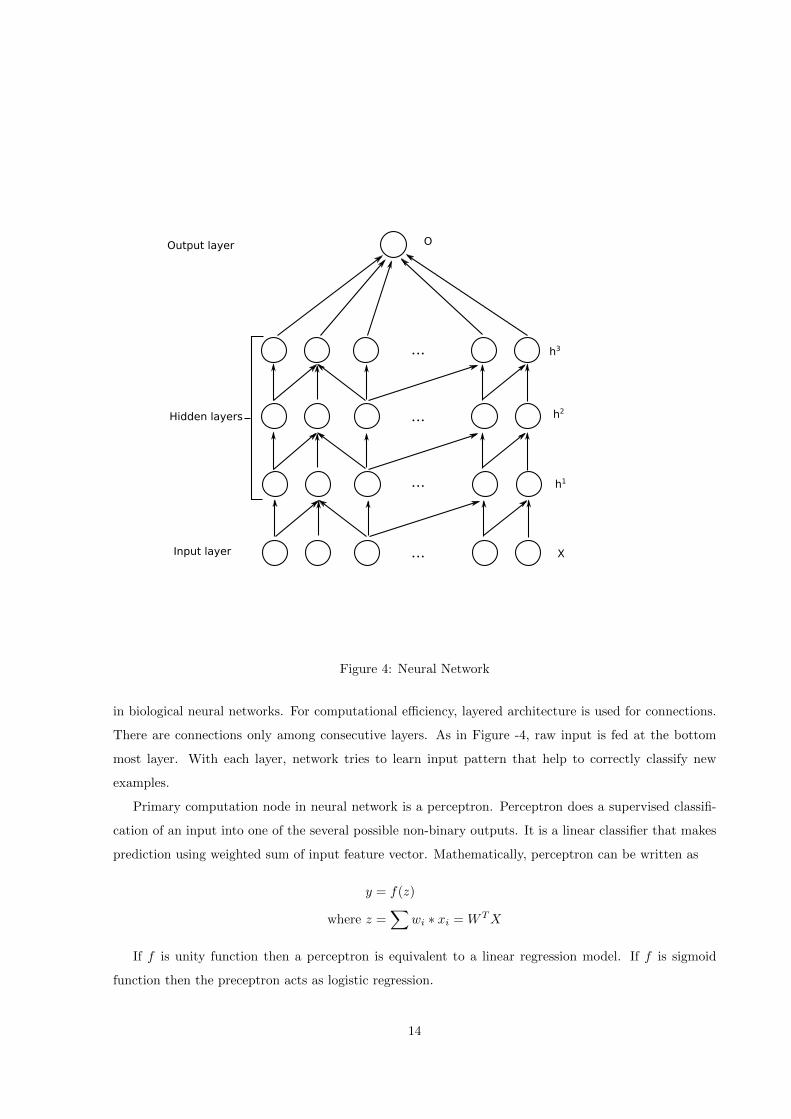
Figure 4: Neural Network

in biological neural networks. For computational efficiency, layered architecture is used for connections.

There are connections only among consecutive layers. As in Figure -4, raw input is fed at the bottom

most layer. With each layer, network tries to learn input pattern that help to correctly classify new

examples.

Primary computation node in neural network is a perceptron. Perceptron does a supervised classifi-

cation of an input into one of the several possible non-binary outputs. It is a linear classifier that makes

prediction using weighted sum of input feature vector. Mathematically, perceptron can be written as

y = f(z)

where z =∑

wi ∗ xi = WTX

If f is unity function then a perceptron is equivalent to a linear regression model. If f is sigmoid

function then the preceptron acts as logistic regression.

14

4.2 Backpropogation algorithm

Backpropogation algorithm, proposed by Rumelhart et al. (1988), is one of the most successful training

algorithm to train a multilayer feed forward network. A backpropogation algorithm learns by example.

Algorithm takes examples as input and it changes the weights in the network links. When the network

is fully trained, it will give the required output for a particular input.

Basic idea of backpropogation algorithm is to minimize the error with respect to input by propogating

error adjustments on the weight of the network. Backpropogation algorithm uses gradient decent method

that calculates the squared error function with respect to the weights of the network. The squared error

function is

E =1

2

∑n∈training

(tn − yn)2

where t = target output

y = actual output of the output node

Now differentiating the above error function gives

δE

δWi=

dE

dyndyn

dznδzn

δWi

Major problems with backpropogation algorithm can be summarized as

• As we backpropogate deep into the network, gradient progressively gets diminished after each layer.

Below certain depth of output neuron, correction signal is very minimal.

• Since the weights are initialized randomly, backpropogation is susceptible to getting stuck local

minima.

• In usual setting, we can only use labeled data. It defeats the motivation for neural network as brain

can learn from unlabeled data.

5 Recent Advances

In this section, we will introduce recent advances in the field of deep learning. New revival of the field is

due to new algorithms that can be learn better features but are trained greedily for a layer. These layers

are then stacked one above the other to learn higher level features. Each layer learns a feature and the

layer above it learns higher level of level of features from the features of the layer below.

In the next section, we will discuss two major methods, autoencoder, denoising autoencoder and Deep

Belief Network(DBN). DBN has probabilistic connotation while autoencoder and denoising autoencoder

are non-probabilistic. These algorithms are usually applied in unsupervised settings but can be modified

for supervised settings.

15

5.1 Autoencoder

An autoencoder neural network is an unsupervised learning algorithm that applies backpropogation

setting target values to be equal to input values. In essence, we try to identity function, so that the input

xs is similar to x. Learning identity function may seem trivial but by applying certain constraints, we

can identify interesting structure about the data.

x1

x2

x3

x4

x5

+1

y1

y2

y3

z5

z4

z3

z2

z1

+1

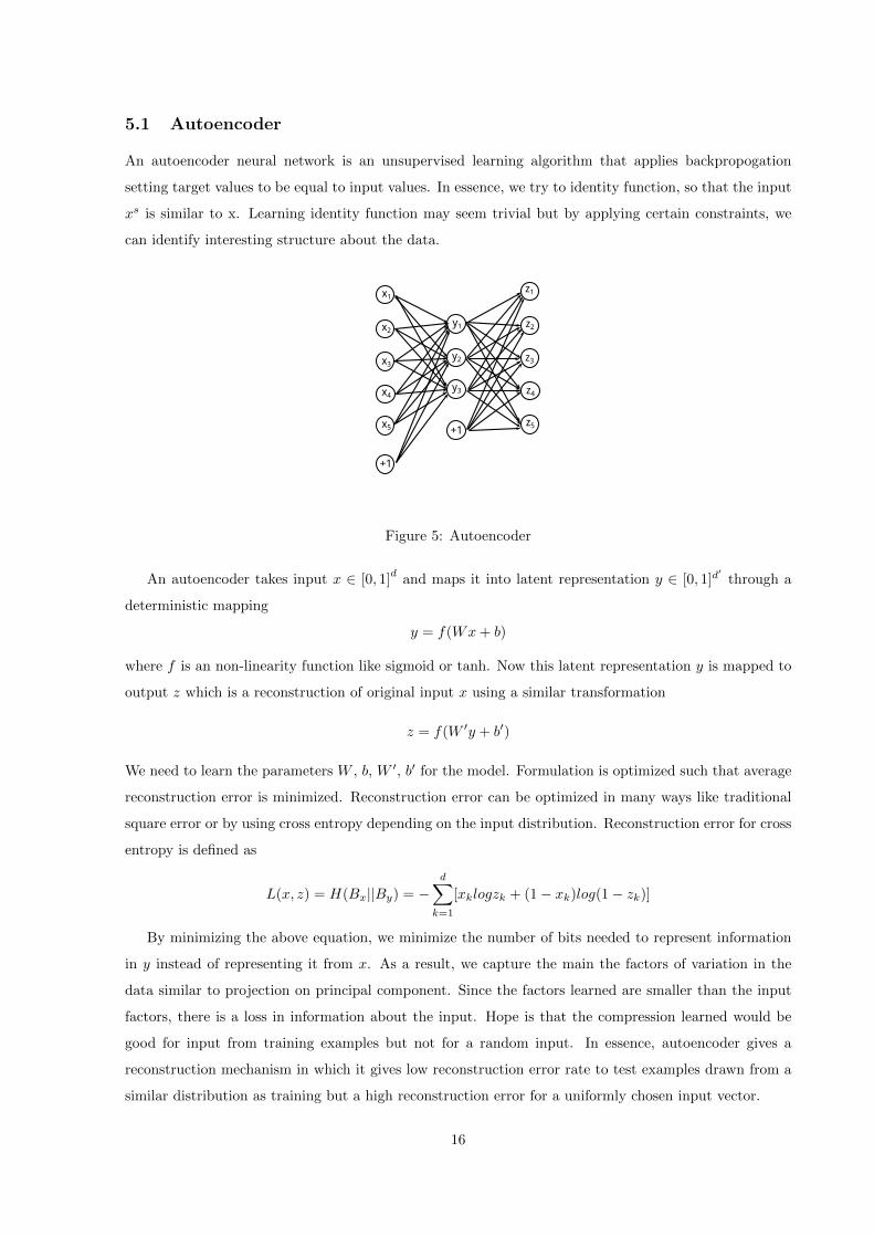
Figure 5: Autoencoder

An autoencoder takes input x ∈ [0, 1]d

and maps it into latent representation y ∈ [0, 1]d′

through a

deterministic mapping

y = f(Wx+ b)

where f is an non-linearity function like sigmoid or tanh. Now this latent representation y is mapped to

output z which is a reconstruction of original input x using a similar transformation

z = f(W ′y + b′)

We need to learn the parameters W , b, W ′, b′ for the model. Formulation is optimized such that average

reconstruction error is minimized. Reconstruction error can be optimized in many ways like traditional

square error or by using cross entropy depending on the input distribution. Reconstruction error for cross

entropy is defined as

L(x, z) = H(Bx||By) = −d∑k=1

[xklogzk + (1− xk)log(1− zk)]

By minimizing the above equation, we minimize the number of bits needed to represent information

in y instead of representing it from x. As a result, we capture the main the factors of variation in the

data similar to projection on principal component. Since the factors learned are smaller than the input

factors, there is a loss in information about the input. Hope is that the compression learned would be

good for input from training examples but not for a random input. In essence, autoencoder gives a

reconstruction mechanism in which it gives low reconstruction error rate to test examples drawn from a

similar distribution as training but a high reconstruction error for a uniformly chosen input vector.

16

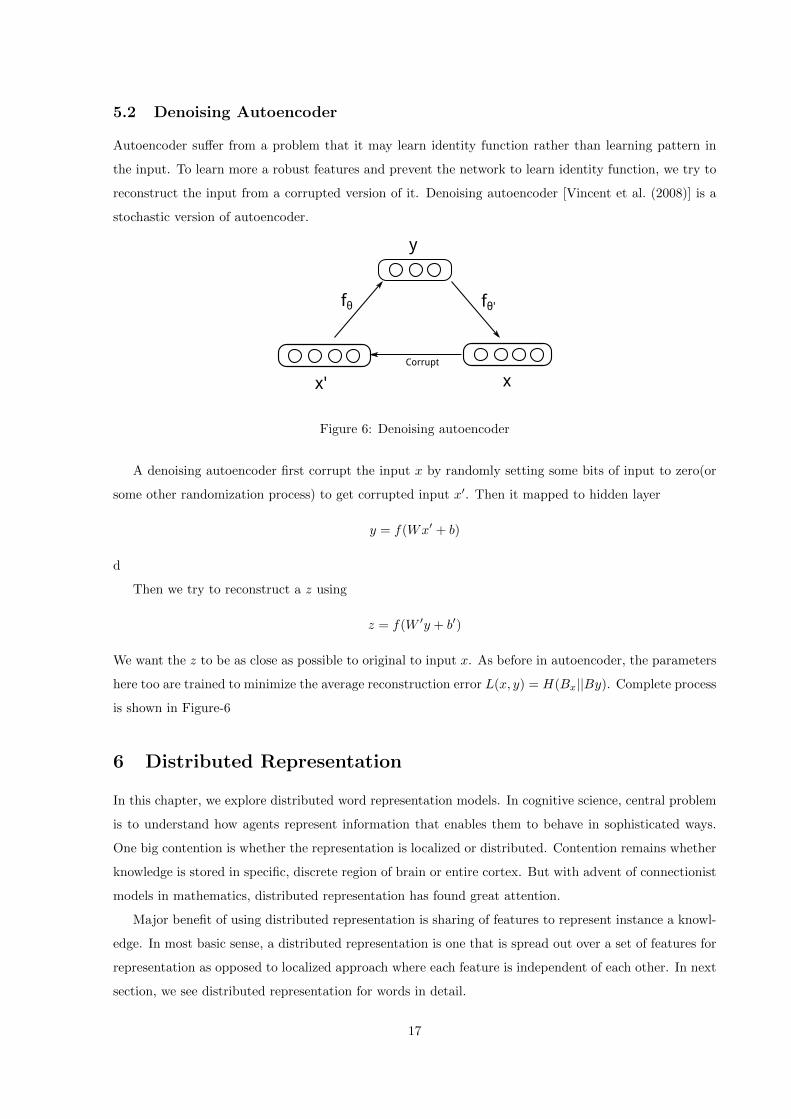
5.2 Denoising Autoencoder

Autoencoder suffer from a problem that it may learn identity function rather than learning pattern in

the input. To learn more a robust features and prevent the network to learn identity function, we try to

reconstruct the input from a corrupted version of it. Denoising autoencoder [Vincent et al. (2008)] is a

stochastic version of autoencoder.

x' x

y

fθ fθ'

Corrupt

Figure 6: Denoising autoencoder

A denoising autoencoder first corrupt the input x by randomly setting some bits of input to zero(or

some other randomization process) to get corrupted input x′. Then it mapped to hidden layer

y = f(Wx′ + b)

d

Then we try to reconstruct a z using

z = f(W ′y + b′)

We want the z to be as close as possible to original to input x. As before in autoencoder, the parameters

here too are trained to minimize the average reconstruction error L(x, y) = H(Bx||By). Complete process

is shown in Figure-6

6 Distributed Representation

In this chapter, we explore distributed word representation models. In cognitive science, central problem

is to understand how agents represent information that enables them to behave in sophisticated ways.

One big contention is whether the representation is localized or distributed. Contention remains whether

knowledge is stored in specific, discrete region of brain or entire cortex. But with advent of connectionist

models in mathematics, distributed representation has found great attention.

Major benefit of using distributed representation is sharing of features to represent instance a knowl-

edge. In most basic sense, a distributed representation is one that is spread out over a set of features for

representation as opposed to localized approach where each feature is independent of each other. In next

section, we see distributed representation for words in detail.

17

6.1 Distributed representation for words

A word representation is a mathematical object associated the each word, often a vector. Each dimension

of the vector represents a feature and might even have a mathematical interpretation. Value of each

dimension represents the amount of activity for that particular feature.

In machine learning, one of the most obvious model of representing a word is one-hot vector repre-

sentation. In this representation only one of the computing element is active for each entity element. For

example, if the size of vocabulary is |V | then word w can be represented as vector of size |V | in which

the index of word w is only active and rest are set to zero.

Home : [0,0,0,0,....,1,....,0,0]

House: [0,0,0,0,..,1,..,0,0,0,0]

This representation is known as local representation. It is easy to understand and implement on

hardware. But this representation has many flaws of itself. As in example shown above, if we want the

correlation between Home and House, the representation fails to show any correlation between the terms.

Lets take an example of POS tagging. We have

Training: ”Dog slept on the mat”

Testing: ”Cat slept on the mat”

By using localized vector representation, these two sentence would have completely different represen-

tation. Hence, a algorithm which has seen only ”Dog” during training would fail to tag ”Cat” during

testing.

Distributed representation would represent these words in some lower dimensional dense vector of

real values with each dimension representing a latent feature for word model. Distributed representation

could be like :

Home : [0.112,0.432,.......,0.341]

House: [0.109,0.459,.......,0.303]

Distributed representation helps to solve the problem of sparsity. For words that are rare in the labeled

training corpus, parameters estimated through one-hot representation will be poor. More over, the model

cannot handle the word that do not appear in the corpus. Distributed representation are trained using

large unlabeled corpus using an unsupervised algorithm. Hope is that the distributed representation

would capture semantic and syntactic properties of word and would have a similar representation for

syntactically and semantically related words.

For example, in the above example of POS tagging, even when we haven’t seen Cat during training,

distributed representation of Cat would be similar to Dog. Algorithm will be able to classify Cat with

similar tag as it would have learned for Dog.

18

6.2 Training distributed word representation

Plethora of methods exists for dimensionality reduction and word representation. Usually, researcher use

clustering for dimensionality reduction. There are mainly two types of clustering algorithms:

• Hard clustering : Class based model learn word classes based on distributional information.

Words are then represented according to the representative of the class. Examples of hard clustering

can be Brown clustering, Exchange clustering etc.

• Soft clustering : Soft clustering models learn for each cluster/topic a distribution over the words

of how likely that word is in each cluster. Examples of soft clustering model are Latent Semantic

Analysis (LSA/LSI), Latent Dirichlet Analysis (LDA), HMM clustering etc.

A continuous space word vector space representation differ significantly from traditional clustering

methods. Words are represented using high dimensional dense vectors in continuous space with no

boundaries. In this study, we mainly focus on vector-space word representation that are learned by input

layer of a neural networks. We will see three different methods based on neural network to learn vector

representation from a large unannotated corpus.

6.2.1 Neural Probabilistic Language Model

Neural Probabilistic Language Model were introduced by Bengio et al. (2003). Method proposed by

Bengio et al. is one of the first methods that introduces word vector representation to capture semantic

similarity between the words. Primary aim of the paper is to develop a language model that overcomes

the curse of dimensionality. For language model to be robust, it needs to generalize over the training

instance. In higher dimensions, it is important how the algorithm distributes it probabilities mass around

the training points. A algorithm performs better if probability mass is distributed where it matter

rather than distributing it in all dimensions uniformly. Neural probabilistic model helps to achieve such

important properties.

In short, the proposed approach can be summarized as follow :

1. associate each word with a distributed word feature vector

2. model the joint probability of word sequences in terms of the feature vectors of the words in sequence

3. learn word vectors and parameters of joint probability function simultaneously

The objective is to learn a good model f(wt, · · · , wt−n+1) = P (wt|wt−11 ) that give high out-of-sample

likelihood. The function f(wt, · · · , wt−n+1) = P (wt|wt−11 ) is decomposed into two parts

1. A mapping C from any element from vocabulary V to a real vector C(i) ∈ Rm. This is the

distributed feature vector associated with every word in vocabulary.

19

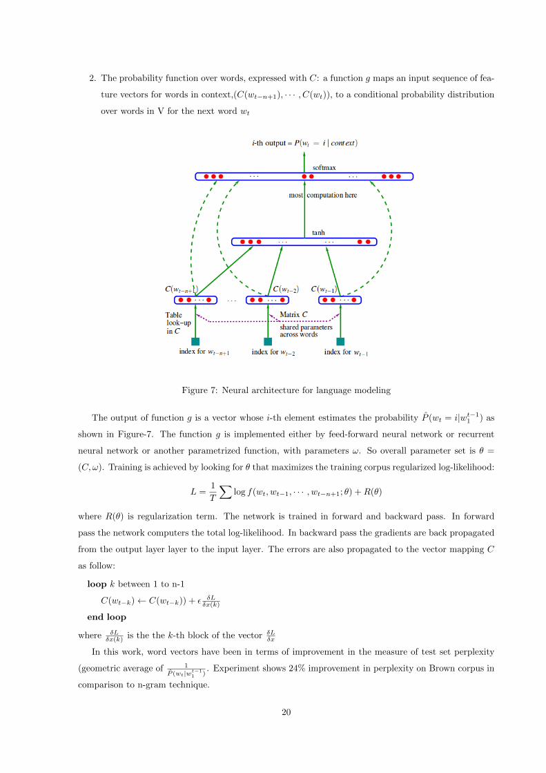
2. The probability function over words, expressed with C: a function g maps an input sequence of fea-

ture vectors for words in context,(C(wt−n+1), · · · , C(wt)), to a conditional probability distribution

over words in V for the next word wt

Figure 7: Neural architecture for language modeling

The output of function g is a vector whose i-th element estimates the probability P (wt = i|wt−11 ) as

shown in Figure-7. The function g is implemented either by feed-forward neural network or recurrent

neural network or another parametrized function, with parameters ω. So overall parameter set is θ =

(C,ω). Training is achieved by looking for θ that maximizes the training corpus regularized log-likelihood:

L =1

T

∑log f(wt, wt−1, · · · , wt−n+1; θ) +R(θ)

where R(θ) is regularization term. The network is trained in forward and backward pass. In forward

pass the network computers the total log-likelihood. In backward pass the gradients are back propagated

from the output layer layer to the input layer. The errors are also propagated to the vector mapping C

as follow:

loop k between 1 to n-1

C(wt−k)← C(wt−k)) + ε δLδx(k)

end loop

where δLδx(k) is the the k-th block of the vector δL

δx

In this work, word vectors have been in terms of improvement in the measure of test set perplexity

(geometric average of 1P (wt|wt−1

1 ). Experiment shows 24% improvement in perplexity on Brown corpus in

comparison to n-gram technique.

20

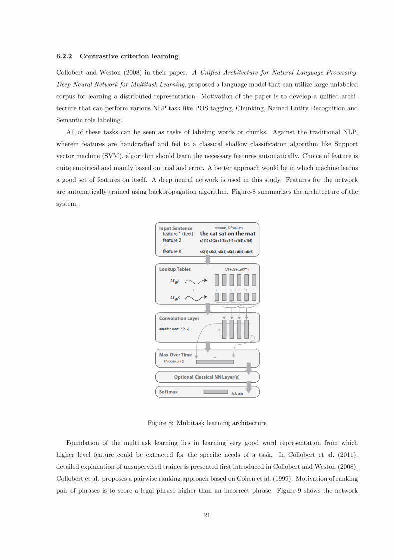
6.2.2 Contrastive criterion learning

Collobert and Weston (2008) in their paper. A Unified Architecture for Natural Language Processing:

Deep Neural Network for Multitask Learning, proposed a language model that can utilize large unlabeled

corpus for learning a distributed representation. Motivation of the paper is to develop a unified archi-

tecture that can perform various NLP task like POS tagging, Chunking, Named Entity Recognition and

Semantic role labeling.

All of these tasks can be seen as tasks of labeling words or chunks. Against the traditional NLP,

wherein features are handcrafted and fed to a classical shallow classification algorithm like Support

vector machine (SVM), algorithm should learn the necessary features automatically. Choice of feature is

quite empirical and mainly based on trial and error. A better approach would be in which machine learns

a good set of features on itself. A deep neural network is used in this study. Features for the network

are automatically trained using backpropagation algorithm. Figure-8 summarizes the architecture of the

system.

Figure 8: Multitask learning architecture

Foundation of the multitask learning lies in learning very good word representation from which

higher level feature could be extracted for the specific needs of a task. In Collobert et al. (2011),

detailed explanation of unsupervised trainer is presented first introduced in Collobert and Weston (2008).

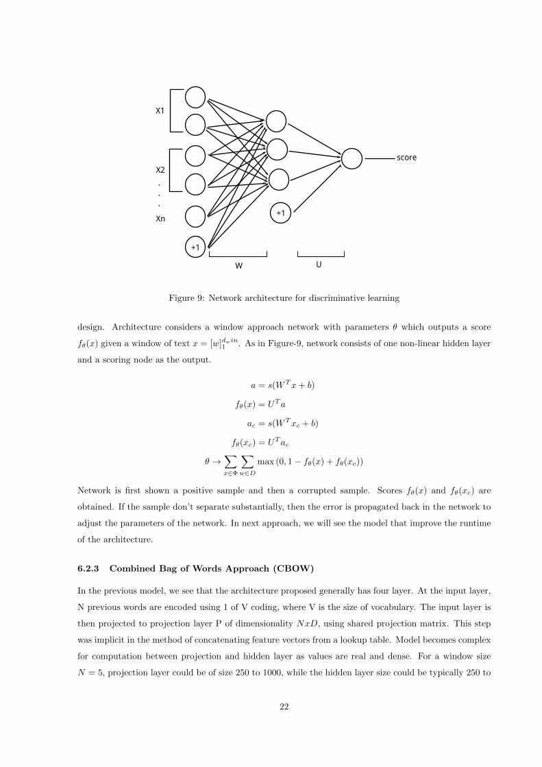
Collobert et al. proposes a pairwise ranking approach based on Cohen et al. (1999). Motivation of ranking

pair of phrases is to score a legal phrase higher than an incorrect phrase. Figure-9 shows the network

21

X1

X2

+1

+1Xn

W U

score

.

.

.

Figure 9: Network architecture for discriminative learning

design. Architecture considers a window approach network with parameters θ which outputs a score

fθ(x) given a window of text x = [w]dwin1 . As in Figure-9, network consists of one non-linear hidden layer

and a scoring node as the output.

a = s(WTx+ b)

fθ(x) = UTa

ac = s(WTxc + b)

fθ(xc) = UTac

θ →∑x∈Φ

∑w∈D

max (0, 1− fθ(x) + fθ(xc))

Network is first shown a positive sample and then a corrupted sample. Scores fθ(x) and fθ(xc) are

obtained. If the sample don’t separate substantially, then the error is propagated back in the network to

adjust the parameters of the network. In next approach, we will see the model that improve the runtime

of the architecture.

6.2.3 Combined Bag of Words Approach (CBOW)

In the previous model, we see that the architecture proposed generally has four layer. At the input layer,

N previous words are encoded using 1 of V coding, where V is the size of vocabulary. The input layer is

then projected to projection layer P of dimensionality NxD, using shared projection matrix. This step

was implicit in the method of concatenating feature vectors from a lookup table. Model becomes complex

for computation between projection and hidden layer as values are real and dense. For a window size

N = 5, projection layer could be of size 250 to 1000, while the hidden layer size could be typically 250 to

22

wt-2

wt-1

wt+1

wt+2

wt

wt-2

wt-1

wt+1

wt+2

wt

projection layer

projection layer

CBOWSkip gram

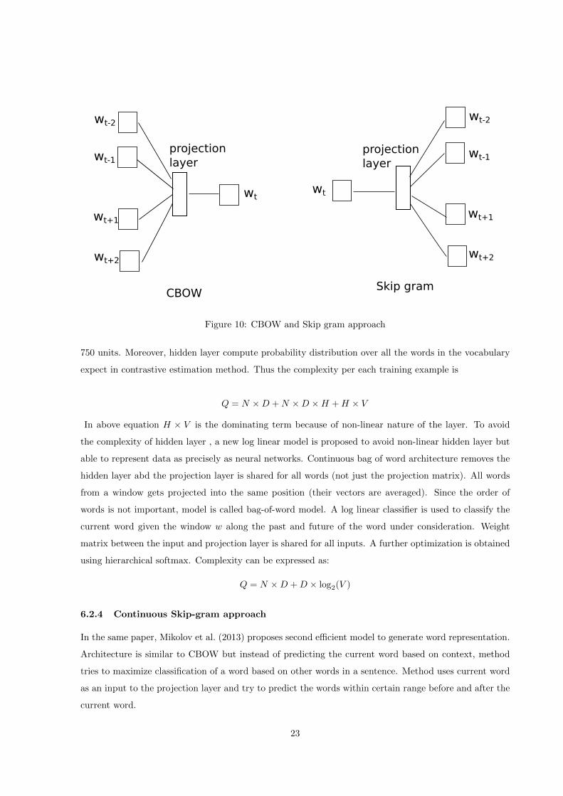
Figure 10: CBOW and Skip gram approach

750 units. Moreover, hidden layer compute probability distribution over all the words in the vocabulary

expect in contrastive estimation method. Thus the complexity per each training example is

Q = N ×D +N ×D ×H +H × V

In above equation H × V is the dominating term because of non-linear nature of the layer. To avoid

the complexity of hidden layer , a new log linear model is proposed to avoid non-linear hidden layer but

able to represent data as precisely as neural networks. Continuous bag of word architecture removes the

hidden layer abd the projection layer is shared for all words (not just the projection matrix). All words

from a window gets projected into the same position (their vectors are averaged). Since the order of

words is not important, model is called bag-of-word model. A log linear classifier is used to classify the

current word given the window w along the past and future of the word under consideration. Weight

matrix between the input and projection layer is shared for all inputs. A further optimization is obtained

using hierarchical softmax. Complexity can be expressed as:

Q = N ×D +D × log2(V )

6.2.4 Continuous Skip-gram approach

In the same paper, Mikolov et al. (2013) proposes second efficient model to generate word representation.

Architecture is similar to CBOW but instead of predicting the current word based on context, method

tries to maximize classification of a word based on other words in a sentence. Method uses current word

as an input to the projection layer and try to predict the words within certain range before and after the

current word.

23

Figure 10 shows the architecture of the model. The complexity of the model can be expressed as :

Q = C × (D +D × log2(V ))

here C is maximum distance from which we want to predict the word. We random choose R between 1

and C and then we use R words from past and R words from the future. Since the words are randomly

chosen we skip some of the words in context and hence the name skip-gram is used for model.

6.3 Semantic and syntactic information in representation

Continuous word representation capture lot of syntactic and syntactic similarities of words in their dense

compact representation. Many linear dependencies among the words are captured using the model

discussed in previous section. As we will show in result section of the report, semantic and syntactic

similarities between the words are well captured by the model. Representation for all the states were

similar in the vector space. All person names , city names were distinctly represented in the space.

Syntactic properties like many inflectional form of word ,viz. dukan and dukhano ,were nearest neighbor

of each other.

Surprisingly, the vectors model has very nice vector properties. We can answer some analogy question

use simple algebraic operations with the vector representation of the words. For example to find a

word, that is similar to small in the same sense as biggest is similar to big, we can simply compute

X = vector(”biggest”)−vector(”big”)+vector(”small”). If we find words with similar representation as

X using cosine similarity and use it to answer the query then it is possible that one of the option would

be ”smallest” among the possibilities.

If large training corpus and big vectors are available and model is trained on them, it is expected

that more semantic and syntactic information could be captured using word representation model. We

may be able to respond to semantic query like analogy among the capitals of countries. For example

, Washington is to USA as Delhi is to India. Word vectors with such semantic properties has lot of

potential application in machine translation, information retrieval, question answering systems and many

other applications.

References

Yoshua Bengio, Rejean Ducharme, Pascal Vincent, and Christian Janvin. A neural probabilistic language

model. J. Mach. Learn. Res., 3:1137–1155, March 2003. ISSN 1532-4435. URL http://dl.acm.org/

citation.cfm?id=944919.944966.

Daniel M. Bikel, Richard Schwartz, and Ralph M. Weischedel. An algorithm that learns whats in a

name. Mach. Learn., 34(1-3):211–231, feb 1999. ISSN 0885-6125. doi: 10.1023/A:1007558221122. URL

http://dx.doi.org/10.1023/A:1007558221122.

24

Andrew Eliot Borthwick. A maximum entropy approach to named entity recognition. PhD thesis, New

York, NY, USA, 1999. AAI9945252.

Xavier Carreras, Lluıs Marquez, and Lluıs Padro. Named entity extraction using adaboost. In proceedings

of the 6th conference on Natural language learning - Volume 20, COLING-02, pages 1–4, Stroudsburg,

PA, USA, 2002. Association for Computational Linguistics. doi: 10.3115/1118853.1118857. URL

http://dx.doi.org/10.3115/1118853.1118857.

William W. Cohen, Robert E. Schapire, and Yoram Singer. Learning to order things. J. Artif. Int. Res.,

10(1):243–270, May 1999. ISSN 1076-9757. URL http://dl.acm.org/citation.cfm?id=1622859.

1622867.

Ronan Collobert and Jason Weston. A unified architecture for natural language processing: deep neural

networks with multitask learning. In Proceedings of the 25th international conference on Machine

learning, ICML ’08, pages 160–167, New York, NY, USA, 2008. ACM. ISBN 978-1-60558-205-4. doi:

10.1145/1390156.1390177. URL http://doi.acm.org/10.1145/1390156.1390177.

Ronan Collobert, Jason Weston, Leon Bottou, Michael Karlen, Koray Kavukcuoglu, and Pavel Kuksa.

Natural language processing (almost) from scratch. J. Mach. Learn. Res., 12:2493–2537, November

2011. ISSN 1532-4435. URL http://dl.acm.org/citation.cfm?id=1953048.2078186.

Corinna Cortes and Vladimir Vapnik. Support-vector networks. In Machine Learning, pages 273–297,

1995.

James R. Curran and Stephen Clark. Language independent ner using a maximum entropy tagger. In

Proceedings of the seventh conference on Natural language learning at HLT-NAACL 2003 - Volume 4,

CONLL ’03, pages 164–167, Stroudsburg, PA, USA, 2003. Association for Computational Linguistics.

doi: 10.3115/1119176.1119200. URL http://dx.doi.org/10.3115/1119176.1119200.

Oren Etzioni, Michael Cafarella, Doug Downey, Ana-Maria Popescu, Tal Shaked, Stephen Soderland,

Daniel S. Weld, and Alexander Yates. Unsupervised named-entity extraction from the web: an

experimental study. Artif. Intell., 165(1):91–134, June 2005. ISSN 0004-3702. doi: 10.1016/j.artint.

2005.03.001. URL http://dx.doi.org/10.1016/j.artint.2005.03.001.

Jr. Forney, G.D. The viterbi algorithm. Proceedings of the IEEE, 61(3):268–278, 1973. ISSN 0018-9219.

doi: 10.1109/PROC.1973.9030.

John D. Lafferty, Andrew McCallum, and Fernando C. N. Pereira. Conditional random fields:

Probabilistic models for segmenting and labeling sequence data. In Proceedings of the Eighteenth

International Conference on Machine Learning, ICML ’01, pages 282–289, San Francisco, CA, USA,

2001. Morgan Kaufmann Publishers Inc. ISBN 1-55860-778-1. URL http://dl.acm.org/citation.

cfm?id=645530.655813.

25

Changki Lee, Yi-Gyu Hwang, Hyo-Jung Oh, Soojong Lim, Jeong Heo, Chung-Hee Lee, Hyeon-Jin Kim,

Ji-Hyun Wang, and Myung-Gil Jang. Fine-grained named entity recognition using conditional random

fields for question answering. In HweeTou Ng, Mun-Kew Leong, Min-Yen Kan, and Donghong Ji,

editors, Information Retrieval Technology, volume 4182 of Lecture Notes in Computer Science, pages

581–587. Springer Berlin Heidelberg, 2006. ISBN 978-3-540-45780-0. doi: 10.1007/11880592 49. URL

http://dx.doi.org/10.1007/11880592_49.

Andrew McCallum and Wei Li. Early results for named entity recognition with conditional random fields,

feature induction and web-enhanced lexicons. In Proceedings of the seventh conference on Natural

language learning at HLT-NAACL 2003 - Volume 4, CONLL ’03, pages 188–191, Stroudsburg, PA,

USA, 2003. Association for Computational Linguistics. doi: 10.3115/1119176.1119206. URL http:

//dx.doi.org/10.3115/1119176.1119206.

Paul McNamee and James Mayfield. Entity extraction without language-specific resources. In proceedings

of the 6th conference on Natural language learning - Volume 20, COLING-02, pages 1–4, Stroudsburg,

PA, USA, 2002. Association for Computational Linguistics. doi: 10.3115/1118853.1118873. URL

http://dx.doi.org/10.3115/1118853.1118873.

Andrei Mikheev, Marc Moens, and Claire Grover. Named entity recognition without gazetteers. In

Proceedings of the Ninth Conference on European Chapter of the Association for Computational

Linguistics, EACL ’99, pages 1–8, Stroudsburg, PA, USA, 1999. Association for Computational

Linguistics. doi: 10.3115/977035.977037. URL http://dx.doi.org/10.3115/977035.977037.

Tomas Mikolov, Kai Chen, Greg Corrado, and Jeffery Dean. Efficient estimation of word representations

in vector space. page to appear, 2013.

Robert Munro and Christopher D. Manning. Accurate unsupervised joint named-entity extraction from

unaligned parallel text. In Proceedings of the 4th Named Entity Workshop, NEWS ’12, pages 21–29,

Stroudsburg, PA, USA, 2012. Association for Computational Linguistics. URL http://dl.acm.org/

citation.cfm?id=2392777.2392781.

David E. Rumelhart, Geoffrey E. Hinton, and Ronald J. Williams. Neurocomputing: foundations of

research. chapter Learning representations by back-propagating errors, pages 696–699. MIT Press,

Cambridge, MA, USA, 1988. ISBN 0-262-01097-6. URL http://dl.acm.org/citation.cfm?id=

65669.104451.

Beth M. Sundheim. Overview of results of the muc-6 evaluation. In Proceedings of the 6th conference

on Message understanding, MUC6 ’95, pages 13–31, Stroudsburg, PA, USA, 1995. Association for

Computational Linguistics. ISBN 1-55860-402-2. doi: 10.3115/1072399.1072402. URL http://dx.

doi.org/10.3115/1072399.1072402.

Pascal Vincent, Hugo Larochelle, Yoshua Bengio, and Pierre-Antoine Manzagol. Extracting and

composing robust features with denoising autoencoders. pages 1096–1103, 2008.

26

GuoDong Zhou and Jian Su. Named entity recognition using an hmm-based chunk tagger. In

Proceedings of the 40th Annual Meeting on Association for Computational Linguistics, ACL ’02,

pages 473–480, Stroudsburg, PA, USA, 2002. Association for Computational Linguistics. doi:

10.3115/1073083.1073163. URL http://dx.doi.org/10.3115/1073083.1073163.

27