Evidence of chaos and nonlinear dynamics in the Peruvian

financial market

Alexis Rodriguez Carranza a, Marco A. P. Cabral bJuan C. Ponte Bejarano c.

aDepartment of Sciences - Private University of the North, Peru

bFederal University of Rio de Janeiro, Brazil

cDepartment of Sciences - Private University of the North, Peru

Resumo

Physicists experimentalists use a large number of observations of a phenomenon, where are the unknown equations thatdescribe it, in order to play the dynamics and obtain information on their future behavior. In this article we study thepossibility of reproducing the dynamics of the phenomenon using only a measurement scale. The Whitney immersion theoremideas are presented and generalization of Sauer for fractal sets to rebuild the asymptotic behaviour of the phenomena and toinvestigate, chaotic behavior evidence in the reproduced dynamics. The applications are made in the financial market whichare only known stock prices

Key words: Caos; Dinamica nao lineal; Series temporais.

1 Introduction

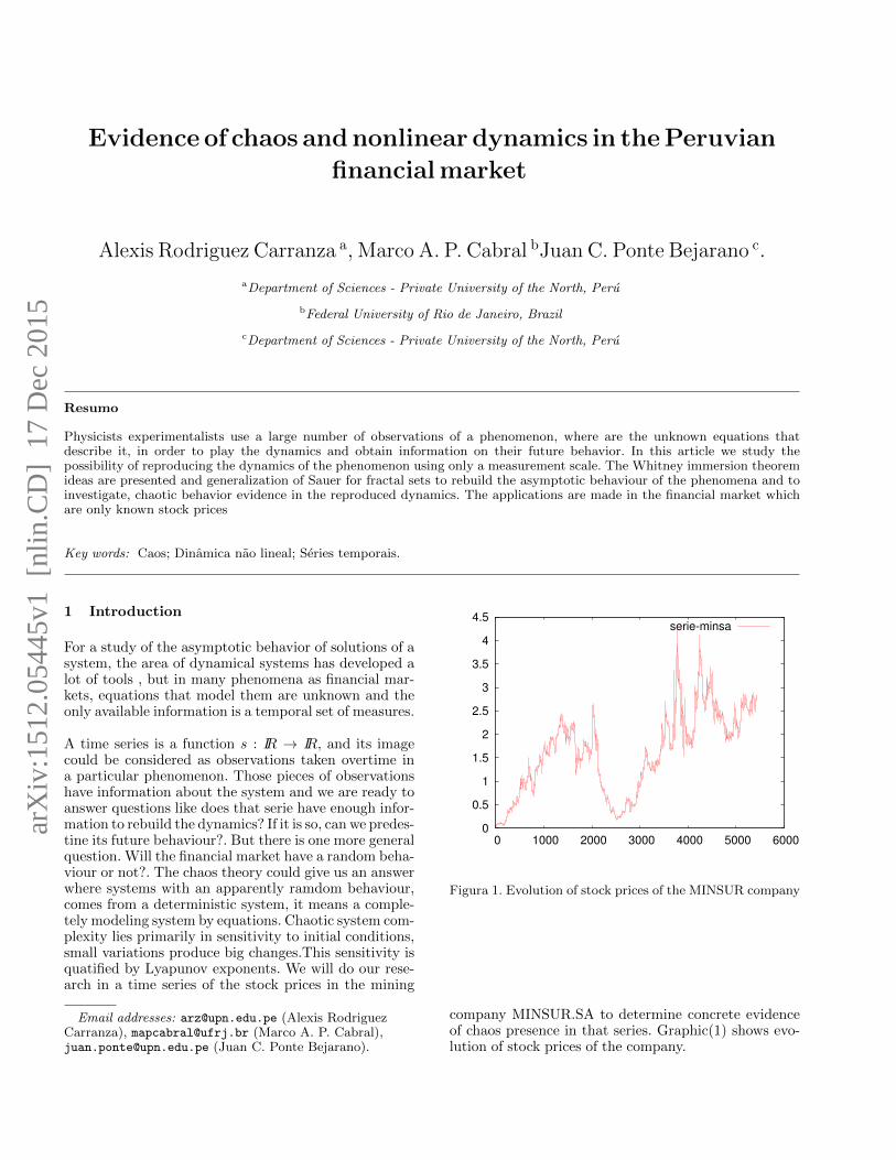
For a study of the asymptotic behavior of solutions of asystem, the area of dynamical systems has developed alot of tools , but in many phenomena as financial mar-kets, equations that model them are unknown and theonly available information is a temporal set of measures.

A time series is a function s : IR → IR, and its imagecould be considered as observations taken overtime ina particular phenomenon. Those pieces of observationshave information about the system and we are ready toanswer questions like does that serie have enough infor-mation to rebuild the dynamics? If it is so, can we predes-tine its future behaviour?. But there is one more generalquestion. Will the financial market have a random beha-viour or not?. The chaos theory could give us an answerwhere systems with an apparently ramdom behaviour,comes from a deterministic system, it means a comple-tely modeling system by equations. Chaotic system com-plexity lies primarily in sensitivity to initial conditions,small variations produce big changes.This sensitivity isquatified by Lyapunov exponents. We will do our rese-arch in a time series of the stock prices in the mining

Email addresses: arz@upn.edu.pe (Alexis RodriguezCarranza), mapcabral@ufrj.br (Marco A. P. Cabral),juan.ponte@upn.edu.pe (Juan C. Ponte Bejarano).

0

0.5

1

1.5

2

2.5

3

3.5

4

4.5

0 1000 2000 3000 4000 5000 6000

serie-minsa

Figura 1. Evolution of stock prices of the MINSUR company

company MINSUR.SA to determine concrete evidenceof chaos presence in that series. Graphic(1) shows evo-lution of stock prices of the company.

arX

iv:1

512.

0544

5v1

[nl

in.C

D]

17

Dec

201

5

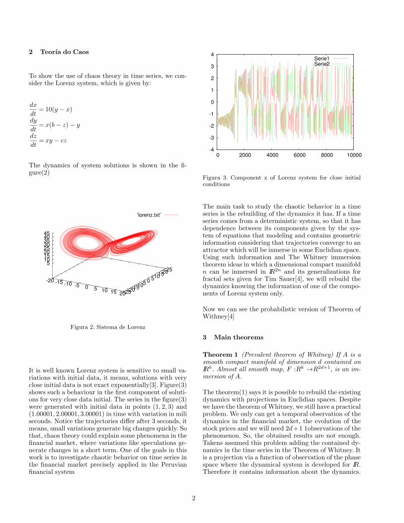
2 Teorıa do Caos

To show the use of chaos theory in time series, we con-sider the Lorenz system, which is given by:

dx

dt= 10(y − x)

dy

dt= x(b− z)− y

dz

dt= xy − cz

The dynamics of system solutions is shown in the fi-gure(2)

-20 -15 -10 -5 0 5 10 15 20-25-20

-15-10

-5 0

5 10

15 20

25

5 10 15 20 25 30 35 40 45

’lorenz.txt’

Figura 2. Sistema de Lorenz

It is well known Lorenz system is sensitive to small va-riations with initial data, it means, solutions with veryclose initial data is not exact exponentially[3]. Figure(3)shows such a behaviour in the first component of soluti-ons for very close data initial. The series in the figure(3)were generated with initial data in points (1, 2, 3) and(1.00001, 2.00001, 3.00001) in time with variation in miliseconds. Notice the trajectories differ after 3 seconds, itmeans, small variations generate big changes quickly. Sothat, chaos theory could explain some phenomena in thefinancial market, where variations like speculations ge-nerate changes in a short term. One of the goals in thiswork is to investigate chaotic behavior on time series inthe financial market precisely applied in the Peruvianfinancial system

-4

-3

-2

-1

0

1

2

3

4

0 2000 4000 6000 8000 10000

Serie1

Serie2

Figura 3. Component x of Lorenz system for close initialconditions

The main task to study the chaotic behavior in a timeseries is the rebuilding of the dynamics it has. If a timeseries comes from a deterministic system, so that it hasdependence between its components given by the sys-tem of equations that modeling and contains geometricinformation considering that trajectories converge to anattractor which will be inmerse in some Euclidian space.Using such information and The Whitney immersiontheorem ideas in which a dimensional compact manifoldn can be inmersed in IR2n and its generalizations forfractal sets given for Tim Sauer[4], we will rebuild thedynamics knowing the information of one of the compo-nents of Lorenz system only.

Now we can see the probabilistic version of Theorem ofWithney[4]

3 Main theorems

Theorem 1 (Prevalent theorem of Whitney) If A is asmooth compact manifold of dimension d contained onIRk. Almost all smooth map, F :Rk →R2d+1, is an im-mersion of A.

The theorem(1) says it is possible to rebuild the existingdynamics with projections in Euclidian spaces. Despitewe have the theorem of Whitney, we still have a practicalproblem. We only can get a temporal observation of thedynamics in the financial market, the evolution of thestock prices and we will need 2d+1 1observations of thephenomenon. So, the obtained results are not enough.Takens assumed this problem adding the contained dy-namics in the time series in the Theorem of Whitney. Itis a projection via a function of observation of the phasespace where the dynamical system is developed for IR.Therefore it contains information about the dynamics.

2

For this, it defines the delay cordinates, which only needa temporary observation.

Definition 2 If Φ is a dynamics system over a manifoldA, T a positive integer (called of delay), and h : A →Ra smoth function. We defines the map of delaying coor-dinates F(Φ,T,h) : A→Rn+1

F(Φ,T,h)(x) = (h(x), h(ΦT (x)), h(Φ2T (x)), . . . , h(ΦnT (x)))

Taken[7] demonstrated a new version of theorem ofWhitney for the delaying coordinates

Theorem 3 (Takens) A is a dimensional compact ma-nifold m, {Φk}k∈Z a discrete dynamical system over Agenerated by F : A → A, and a function of classe C2

h : A → IR. is a generic characteristic that of mapF(Φ,h)(x) : A→ IR2m+1 defined by

F(Φ,h)(x) = (h(x), h(Φk(x)), h(Φ2k(x)), . . . , h(Φnk(x)))

is an immersion.

The final generalization used in this article was givenby B.Hunt, T. Sauer and J. Yorke[8], that is a fractalversion of theorem of Whitney for the delaying maps setwith A being a fractal set.

Theorem 4 (Fractal Delay Embedding Prevalence The-orem) Φ A dynamics system over an open subset U ofIRk, and A a compact subset of U with box dimension d.n > 2d an integer and T > 0. Asume thatA contains onlya finite number of equilibrio points, it does not containsperiodic orbits of Φ of period T o 2T , a finit number ofperiodic orbits of Φ of period 3T , 4T, . . . , nT , and theseperiodic orbits linearizations have different eigenvalues.So for almost every smooth function(in the sense preva-lente) smooth function h over U , the delay coordinatesmap F(Φ,T,h) : U →Rn is injective over A

The theorem(4) does not provide an estimative aboutthe smaller dimension for which almost every delayingcoordinates map is injective. However there are nume-rical algorithms which allow calculate the immersiondimension and the delaying time in the reconstruc-tion.Following, we show the reconstruction of the dyna-mics generated for the system of Lorenz using only thecoordinate x of the system

4 4. Examples of reconstruction of the attractorusing delay coordinates

we use the Lorenz’s attractor to show the technique ofdelaying coordinates. The function of observation h, was

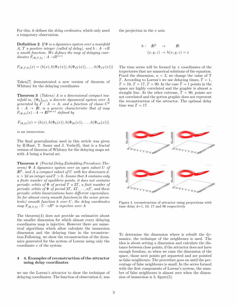
the projection in the x axis.

h : IR3 → IR

(x, y, z) → h(x, y, z) = x

The time series will be formed by x coordinates of thetrajectories that are numerical solutions of the equation.Fixed the dimension, n = 3, we change the value of TT . According to Lorenz’s we use delaying times, T = 1,T = 10, T = 17, T = 90. In the case T = 1 points in thespace are highly correlated and the graphic is almost astraight line. At the other extreme, T = 90, points arenot correlated and the gotten graphic does not representthe reconstruction of the attractor. The optimal delaytime was T = 17.

-20 -15 -10 -5 0 5 10 15 20-25-20

-15-10

-5 0

5 10

15 20

25

-20-10

0 10 20 30 40 50

-20 -15 -10 -5 0 5 10 15 20-25-20

-15-10

-5 0

5 10

15 20

25

-20-10

0 10 20 30 40 50

-20 -15 -10 -5 0 5 10 15 20-25-20

-15-10

-5 0

5 10

15 20

25

-20-10

0 10 20 30 40 50

-20 -15 -10 -5 0 5 10 15 20-25-20

-15-10

-5 0

5 10

15 20

25

-20-10

0 10 20 30 40 50

Figura 4. reconstruction of attractor using proyections withtime delay d=1, 10, 17 and 90 respectively

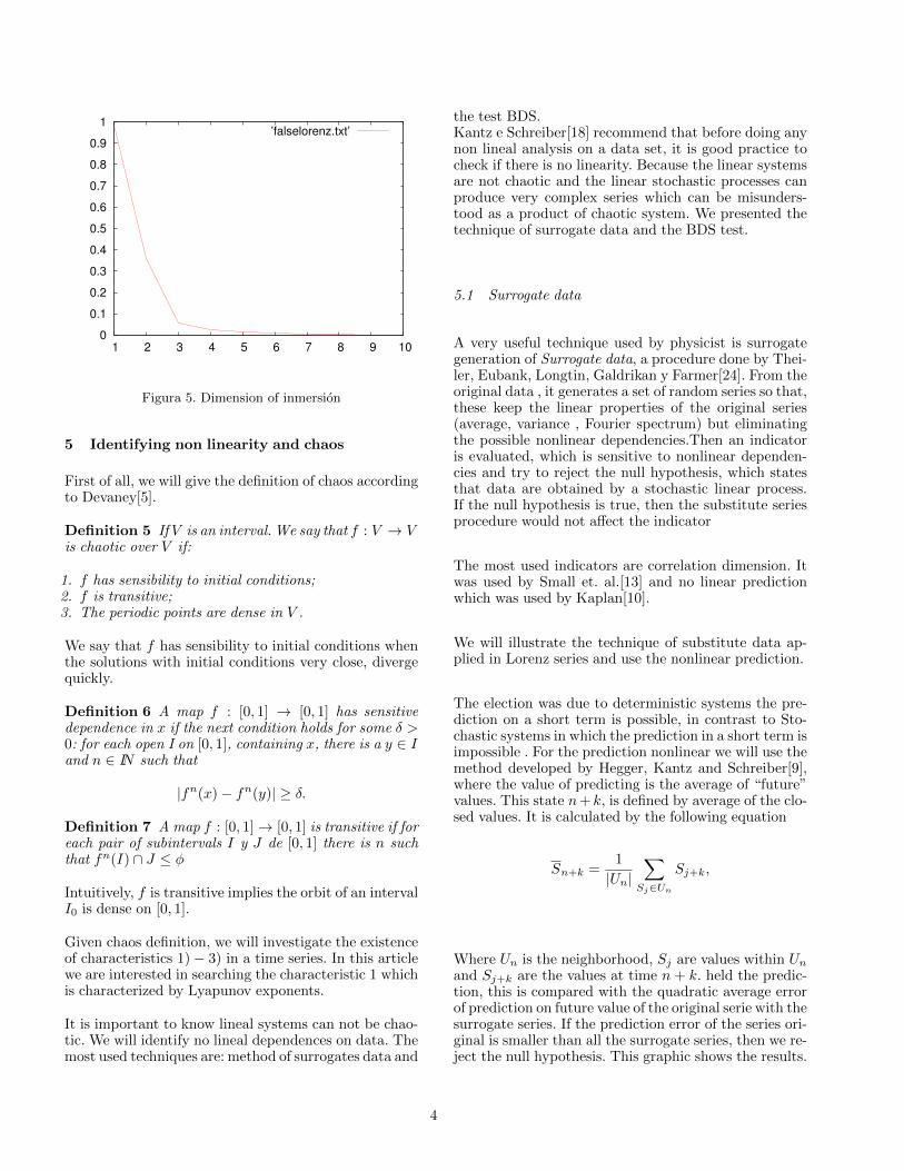
To determine the dimension where is rebuilt the dy-namics, the technique of the neighbours is used. Theidea is about setting a dimension and calculate the dis-tance between close points, if the attractor does not haveenough freedom, so when we raise the dimension of thespace, those next points get separeted and are pointedas false neighbours. The procedure goes on until the per-centage of false neighbours is small. In the series formedwith the first components of Lorenz’s system, the num-ber of false neighbours is almost zero when the dimen-sion of immersion is 3, figure(5).

3

0

0.1

0.2

0.3

0.4

0.5

0.6

0.7

0.8

0.9

1

1 2 3 4 5 6 7 8 9 10

’falselorenz.txt’

Figura 5. Dimension of inmersion

5 Identifying non linearity and chaos

First of all, we will give the definition of chaos accordingto Devaney[5].

Definition 5 If V is an interval. We say that f : V → Vis chaotic over V if:

1. f has sensibility to initial conditions;2. f is transitive;3. The periodic points are dense in V .

We say that f has sensibility to initial conditions whenthe solutions with initial conditions very close, divergequickly.

Definition 6 A map f : [0, 1] → [0, 1] has sensitivedependence in x if the next condition holds for some δ >0: for each open I on [0, 1], containing x, there is a y ∈ Iand n ∈ IN such that

|fn(x)− fn(y)| ≥ δ.

Definition 7 A map f : [0, 1]→ [0, 1] is transitive if foreach pair of subintervals I y J de [0, 1] there is n suchthat fn(I) ∩ J ≤ φ

Intuitively, f is transitive implies the orbit of an intervalI0 is dense on [0, 1].

Given chaos definition, we will investigate the existenceof characteristics 1)− 3) in a time series. In this articlewe are interested in searching the characteristic 1 whichis characterized by Lyapunov exponents.

It is important to know lineal systems can not be chao-tic. We will identify no lineal dependences on data. Themost used techniques are: method of surrogates data and

the test BDS.Kantz e Schreiber[18] recommend that before doing anynon lineal analysis on a data set, it is good practice tocheck if there is no linearity. Because the linear systemsare not chaotic and the linear stochastic processes canproduce very complex series which can be misunders-tood as a product of chaotic system. We presented thetechnique of surrogate data and the BDS test.

5.1 Surrogate data

A very useful technique used by physicist is surrogategeneration of Surrogate data, a procedure done by Thei-ler, Eubank, Longtin, Galdrikan y Farmer[24]. From theoriginal data , it generates a set of random series so that,these keep the linear properties of the original series(average, variance , Fourier spectrum) but eliminatingthe possible nonlinear dependencies.Then an indicatoris evaluated, which is sensitive to nonlinear dependen-cies and try to reject the null hypothesis, which statesthat data are obtained by a stochastic linear process.If the null hypothesis is true, then the substitute seriesprocedure would not affect the indicator

The most used indicators are correlation dimension. Itwas used by Small et. al.[13] and no linear predictionwhich was used by Kaplan[10].

We will illustrate the technique of substitute data ap-plied in Lorenz series and use the nonlinear prediction.

The election was due to deterministic systems the pre-diction on a short term is possible, in contrast to Sto-chastic systems in which the prediction in a short term isimpossible . For the prediction nonlinear we will use themethod developed by Hegger, Kantz and Schreiber[9],where the value of predicting is the average of “future”values. This state n+ k, is defined by average of the clo-sed values. It is calculated by the following equation

Sn+k =1

|Un|∑Sj∈Un

Sj+k,

Where Un is the neighborhood, Sj are values within Unand Sj+k are the values at time n + k. held the predic-tion, this is compared with the quadratic average errorof prediction on future value of the original serie with thesurrogate series. If the prediction error of the series ori-ginal is smaller than all the surrogate series, then we re-ject the null hypothesis. This graphic shows the results.

4

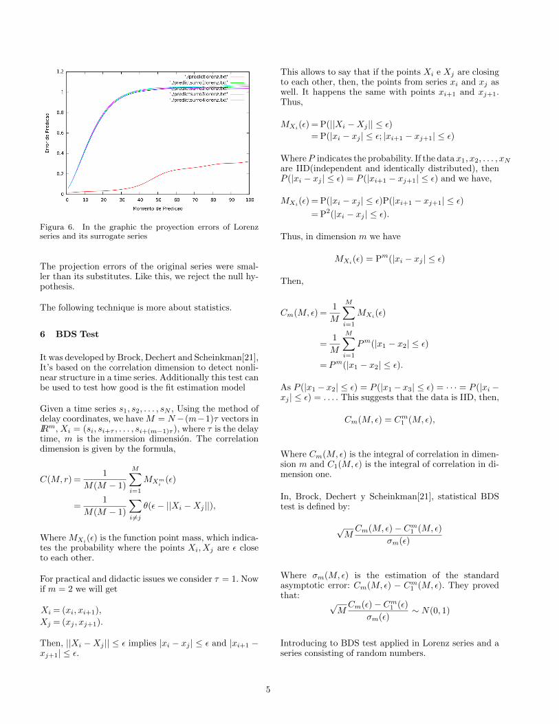
Figura 6. In the graphic the proyection errors of Lorenzseries and its surrogate series

The projection errors of the original series were smal-ler than its substitutes. Like this, we reject the null hy-pothesis.

The following technique is more about statistics.

6 BDS Test

It was developed by Brock, Dechert and Scheinkman[21],It’s based on the correlation dimension to detect nonli-near structure in a time series. Additionally this test canbe used to test how good is the fit estimation model

Given a time series s1, s2, . . . , sN , Using the method ofdelay coordinates, we have M = N−(m−1)τ vectors inIRm, Xi = (si, si+τ , . . . , si+(m−1)τ ), where τ is the delaytime, m is the immersion dimension. The correlationdimension is given by the formula,

C(M, r) =1

M(M − 1)

M∑i=1

MXmi

(ε)

=1

M(M − 1)

∑i 6=j

θ(ε− ||Xi −Xj ||),

Where MXi(ε) is the function point mass, which indica-

tes the probability where the points Xi, Xj are ε closeto each other.

For practical and didactic issues we consider τ = 1. Nowif m = 2 we will get

Xi = (xi, xi+1),

Xj = (xj , xj+1).

Then, ||Xi −Xj || ≤ ε implies |xi − xj | ≤ ε and |xi+1 −xj+1| ≤ ε.

This allows to say that if the points Xi e Xj are closingto each other, then, the points from series xi and xj aswell. It happens the same with points xi+1 and xj+1.Thus,

MXi(ε) = P(||Xi −Xj || ≤ ε)

= P(|xi − xj | ≤ ε; |xi+1 − xj+1| ≤ ε)

WhereP indicates the probability. If the data x1, x2, . . . , xNare IID(independent and identically distributed), thenP (|xi − xj | ≤ ε) = P (|xi+1 − xj+1| ≤ ε) and we have,

MXi(ε) = P(|xi − xj | ≤ ε)P(|xi+1 − xj+1| ≤ ε)

= P2(|xi − xj | ≤ ε).

Thus, in dimension m we have

MXi(ε) = Pm(|xi − xj | ≤ ε)

Then,

Cm(M, ε) =1

M

M∑i=1

MXi(ε)

=1

M

M∑i=1

Pm(|x1 − x2| ≤ ε)

= Pm(|x1 − x2| ≤ ε).

As P (|x1 − x2| ≤ ε) = P (|x1 − x3| ≤ ε) = · · · = P (|xi −xj | ≤ ε) = . . . . This suggests that the data is IID, then,

Cm(M, ε) = Cm1 (M, ε),

Where Cm(M, ε) is the integral of correlation in dimen-sion m and C1(M, ε) is the integral of correlation in di-mension one.

In, Brock, Dechert y Scheinkman[21], statistical BDStest is defined by:

√MCm(M, ε)− Cm1 (M, ε)

σm(ε)

Where σm(M, ε) is the estimation of the standardasymptotic error: Cm(M, ε) − Cm1 (M, ε). They provedthat:

√MCm(ε)− Cm1 (ε)

σm(ε)∼ N(0, 1)

Introducing to BDS test applied in Lorenz series and aseries consisting of random numbers.

5

6.1 BDS Test for Lorenz series

Dimension of immersion(m) BDS

1 165.270466

2 447.623951

3 578.535241

4 772.617763

5 1078.467687

6 2338.679429

7 3593.653394

8 5640.618871

6.2 Test BDS for a series consisting of random numbers

Dimension of immersion(m) BDS

1 0.560594

2 0.560594

3 0.425293

4 0.069765

5 0.116118

6 0.336857

7 0.633835

8 0.524584

To understand the results, let’s start talking about thedegree of significance of a hypothesis. To ask a null hy-pothesis, in the case of the BDS test the null hypothesisis that the observations are independent and identicallydistributed (IID), it can be make a mistake of rejectingthe null hypothesis being true. Suppose that the proba-bility of committing this error is α, namely:

α = P (rejeitar H0|H0 e verdadeiro)

α is called the degree of significance of this mistake. Now,in the BDS test:

H0 : Cm(M, ε) =Cm1 (M, ε)

Ha : Cm(M, ε) 6=Cm1 (M, ε)

By the test BDS, know that

√MCm(M, ε)− Cm1 (M, ε)

σm(ε)∼ N(0, 1)

Then,

α = P (rejeitar H0|H0 everdadeiro)

α = P (|√MCm(M, ε)− Cm1 (M, ε)

σm(ε)| > zc|H0 e verdadeiro)

α = P (|√MCm(M, ε)− Cm1 (M, ε)

σm(ε)| > zc ∼ N(0, 1))

α = 1− 2P (0 ≤√MCm(M, ε)− Cm1 (M, ε)

σm(ε)≤ zc)

So,

P (0 ≤√MCm(M, ε)− Cm1 (M, ε)

σm(ε)≤ zc) =

1− α2

If we look at the tables of the normal distribu-tion N(0, 1), we see that you to a degree of signi-cancia of α = 5%, zc = 1.96. As, we reject thenull hypothesis, with degree of signicancia of 5%, if

|√M Cm(ε)−C1m(ε)

σm(ε) | > 1.96. Noting again the tables we

can observe that in the case of Lorenz series, we rejectthe null hypothesis, the data are IID. Otherwise caseseries formed by random numbers.

Detected non-linealidade in the time series, the next stepis to search sensitive dependence on initial conditions.

6.3 Lyapunov exponents

This section we obtain results that characterize the sen-sitive dependence on initial conditions. The study of theattractor and the dynamics is performed in the spacereconstructed using delay coordinates.

This section we obtain results that characterize the sen-sitive dependence on initial conditions. The study of theattractor and the dynamics is performed in the spacereconstructed using delay coordinates. Chaotic systemsare, generally, strange attractors which are generatedby stretching and contractions. Stretches are responsi-ble for sensitivity on initial conditions and are charac-terized by the exponential distance in finite time, pathswith initial conditions very next. Contractions allow thepathlines may not move away indefinitely and that theyremain confined to a bounded phase space region. Dis-tance speed is measured by the Lyapunov exponents.

In the case of a discrete dynamic defined by a map systemf :Rn →Rn,

T (x) = Dxf

6

is the Jacobian matrix of f . then writing

T (x) = Tnx = T (fn−1x), . . . , T (fx), T (x)

The largest Lyapunov exponent is given by:

λ1 = limn→∞

1

n||Tnx u||

for almost all vector u, for more details see[6]. As wecan see the first problem for the calculation of Lyapunovexponents is to obtain the matrizes T (x) = Dxf . Inthe case of having only a time series the calculation ofLyapunov exponent is even more complicated. Eckmany Ruelle[6],[16] proposed the first algorithms based onthe following ideas.

Consider a dynamic generated by the differential equa-tion:

dx(t)

dt= F (x(t)) (1)

In IRn. If we do u(t) = F (x(t)) in the previous equalitywe get,

du(t)

dt= (Dx(t)F )(u(t)). (2)

The retrieved system is linear in u. Then, if the system(1)solutions are x(t) = f t(x(0)), then the solutions of thesystem(2) are u(t) = (Dx(0)f

t)u(0). So the matrix, T xt =Dxf

t, can be calculated integrating the equations (1).This idea for a linear system to calculate the matrix,T xt = Dxf

t, was used by Eckman and Ruelle[16] forestimating of Lyapunov exponents from a time series.

Consider a time series, s1, s2, . . . , sn. Using delay coor-dinates, obtain points X1, X2, . . . , Xm, in the space m-dimensional of reconstruction. If we develop f aroundpoint xi, we would have that for xj next to it,

f(Xj)≈ f(Xi) +DfXi(Xj −Xi)

f(Xj)− f(Xi)≈DfXi(Xj −Xi) (3)

So, TX(i)τ = DX(i)f

τ is estimated by the best linear ap-proximation of the map that for points x(j) next to pointX(i), takesX(j)−X(i) in points fτ (X(j))−fτ (X(i)) =X(j + τ)−X(i+ τ) close. This process can be thoughtas the linear approximation of the derivatives at eachpoint in space lathe overhauled do. With the same ideas,authors such as Wolf, Swift, Swinney Vastano[22], M.Sano, y. Sawada[20] proposed an algorithm for the cal-culation of Lyapunov exponents.

Another factor to consider is that the Lyapunov expo-nents are defined in terms of limits, which guaranteesits invariance by smooth transformations. If we think

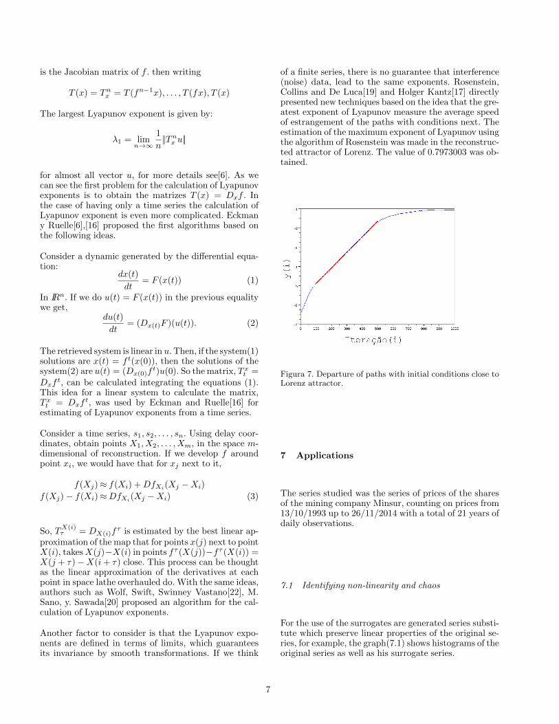
of a finite series, there is no guarantee that interference(noise) data, lead to the same exponents. Rosenstein,Collins and De Luca[19] and Holger Kantz[17] directlypresented new techniques based on the idea that the gre-atest exponent of Lyapunov measure the average speedof estrangement of the paths with conditions next. Theestimation of the maximum exponent of Lyapunov usingthe algorithm of Rosenstein was made in the reconstruc-ted attractor of Lorenz. The value of 0.7973003 was ob-tained.

Figura 7. Departure of paths with initial conditions close toLorenz attractor.

7 Applications

The series studied was the series of prices of the sharesof the mining company Minsur, counting on prices from13/10/1993 up to 26/11/2014 with a total of 21 years ofdaily observations.

7.1 Identifying non-linearity and chaos

For the use of the surrogates are generated series substi-tute which preserve linear properties of the original se-ries, for example, the graph(7.1) shows histograms of theoriginal series as well as his surrogate series.

7

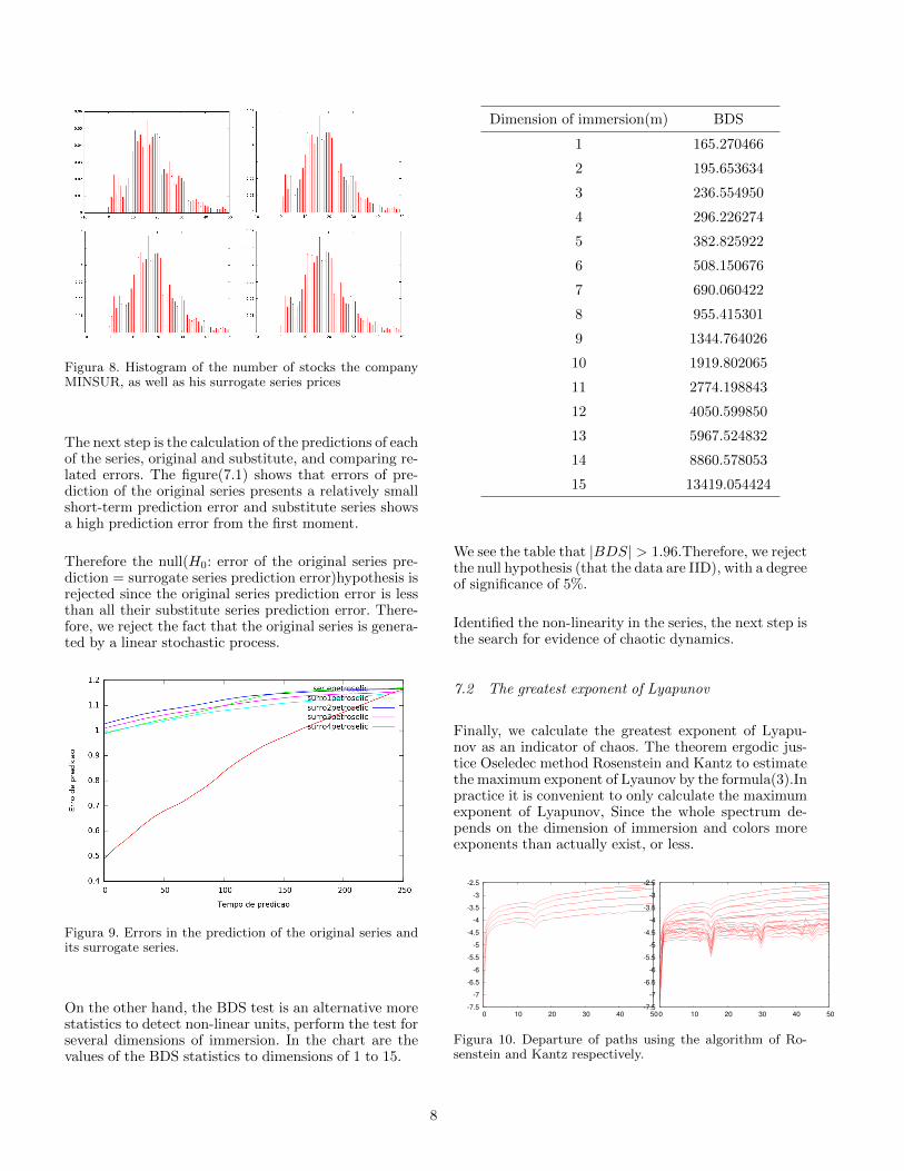
Figura 8. Histogram of the number of stocks the companyMINSUR, as well as his surrogate series prices

The next step is the calculation of the predictions of eachof the series, original and substitute, and comparing re-lated errors. The figure(7.1) shows that errors of pre-diction of the original series presents a relatively smallshort-term prediction error and substitute series showsa high prediction error from the first moment.

Therefore the null(H0: error of the original series pre-diction = surrogate series prediction error)hypothesis isrejected since the original series prediction error is lessthan all their substitute series prediction error. There-fore, we reject the fact that the original series is genera-ted by a linear stochastic process.

Figura 9. Errors in the prediction of the original series andits surrogate series.

On the other hand, the BDS test is an alternative morestatistics to detect non-linear units, perform the test forseveral dimensions of immersion. In the chart are thevalues of the BDS statistics to dimensions of 1 to 15.

Dimension of immersion(m) BDS

1 165.270466

2 195.653634

3 236.554950

4 296.226274

5 382.825922

6 508.150676

7 690.060422

8 955.415301

9 1344.764026

10 1919.802065

11 2774.198843

12 4050.599850

13 5967.524832

14 8860.578053

15 13419.054424

We see the table that |BDS| > 1.96.Therefore, we rejectthe null hypothesis (that the data are IID), with a degreeof significance of 5%.

Identified the non-linearity in the series, the next step isthe search for evidence of chaotic dynamics.

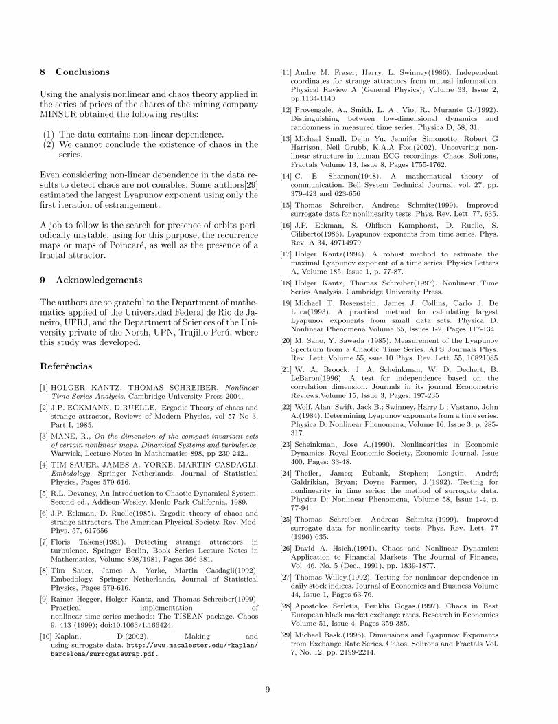
7.2 The greatest exponent of Lyapunov

Finally, we calculate the greatest exponent of Lyapu-nov as an indicator of chaos. The theorem ergodic jus-tice Oseledec method Rosenstein and Kantz to estimatethe maximum exponent of Lyaunov by the formula(3).Inpractice it is convenient to only calculate the maximumexponent of Lyapunov, Since the whole spectrum de-pends on the dimension of immersion and colors moreexponents than actually exist, or less.

-7.5

-7

-6.5

-6

-5.5

-5

-4.5

-4

-3.5

-3

-2.5

0 10 20 30 40 50

-7.5

-7

-6.5

-6

-5.5

-5

-4.5

-4

-3.5

-3

-2.5

0 10 20 30 40 50

Figura 10. Departure of paths using the algorithm of Ro-senstein and Kantz respectively.

8

8 Conclusions

Using the analysis nonlinear and chaos theory applied inthe series of prices of the shares of the mining companyMINSUR obtained the following results:

(1) The data contains non-linear dependence.(2) We cannot conclude the existence of chaos in the

series.

Even considering non-linear dependence in the data re-sults to detect chaos are not conables. Some authors[29]estimated the largest Lyapunov exponent using only thefirst iteration of estrangement.

A job to follow is the search for presence of orbits peri-odically unstable, using for this purpose, the recurrencemaps or maps of Poincare, as well as the presence of afractal attractor.

9 Acknowledgements

The authors are so grateful to the Department of mathe-matics applied of the Universidad Federal de Rio de Ja-neiro, UFRJ, and the Department of Sciences of the Uni-versity private of the North, UPN, Trujillo-Peru, wherethis study was developed.

Referencias

[1] HOLGER KANTZ, THOMAS SCHREIBER, NonlinearTime Series Analysis. Cambridge University Press 2004.

[2] J.P. ECKMANN, D.RUELLE, Ergodic Theory of chaos andstrange attractor, Reviews of Modern Physics, vol 57 No 3,Part I, 1985.

[3] MANE, R., On the dimension of the compact invariant setsof certain nonlinear maps. Dinamical Systems and turbulence.Warwick, Lecture Notes in Mathematics 898, pp 230-242..

[4] TIM SAUER, JAMES A. YORKE, MARTIN CASDAGLI,Embedology. Springer Netherlands, Journal of StatisticalPhysics, Pages 579-616.

[5] R.L. Devaney, An Introduction to Chaotic Dynamical System,Second ed., Addison-Wesley, Menlo Park California, 1989.

[6] J.P. Eckman, D. Ruelle(1985). Ergodic theory of chaos andstrange attractors. The American Physical Society. Rev. Mod.Phys. 57, 617656

[7] Floris Takens(1981). Detecting strange attractors inturbulence. Springer Berlin, Book Series Lecture Notes inMathematics, Volume 898/1981, Pages 366-381.

[8] Tim Sauer, James A. Yorke, Martin Casdagli(1992).Embedology. Springer Netherlands, Journal of StatisticalPhysics, Pages 579-616.

[9] Rainer Hegger, Holger Kantz, and Thomas Schreiber(1999).Practical implementation ofnonlinear time series methods: The TISEAN package. Chaos9, 413 (1999); doi:10.1063/1.166424.

[10] Kaplan, D.(2002). Making andusing surrogate data. http://www.macalester.edu/~kaplan/

barcelona/surrogatewrap.pdf.

[11] Andre M. Fraser, Harry. L. Swinney(1986). Independentcoordinates for strange attractors from mutual information.Physical Review A (General Physics), Volume 33, Issue 2,pp.1134-1140

[12] Provenzale, A., Smith, L. A., Vio, R., Murante G.(1992).Distinguishing between low-dimensional dynamics andrandomness in measured time series. Physica D, 58, 31.

[13] Michael Small, Dejin Yu, Jennifer Simonotto, Robert GHarrison, Neil Grubb, K.A.A Fox.(2002). Uncovering non-linear structure in human ECG recordings. Chaos, Solitons,Fractals Volume 13, Issue 8, Pages 1755-1762.

[14] C. E. Shannon(1948). A mathematical theory ofcommunication. Bell System Technical Journal, vol. 27, pp.379-423 and 623-656

[15] Thomas Schreiber, Andreas Schmitz(1999). Improvedsurrogate data for nonlinearity tests. Phys. Rev. Lett. 77, 635.

[16] J.P. Eckman, S. Oliffson Kamphorst, D. Ruelle, S.Ciliberto(1986). Lyapunov exponents from time series. Phys.Rev. A 34, 49714979

[17] Holger Kantz(1994). A robust method to estimate themaximal Lyapunov exponent of a time series. Physics LettersA, Volume 185, Issue 1, p. 77-87.

[18] Holger Kantz, Thomas Schreiber(1997). Nonlinear TimeSeries Analysis. Cambridge University Press.

[19] Michael T. Rosenstein, James J. Collins, Carlo J. DeLuca(1993). A practical method for calculating largestLyapunov exponents from small data sets. Physica D:Nonlinear Phenomena Volume 65, Issues 1-2, Pages 117-134

[20] M. Sano, Y. Sawada (1985). Measurement of the LyapunovSpectrum from a Chaotic Time Series. APS Journals Phys.Rev. Lett. Volume 55, ssue 10 Phys. Rev. Lett. 55, 10821085

[21] W. A. Broock, J. A. Scheinkman, W. D. Dechert, B.LeBaron(1996). A test for independence based on thecorrelation dimension. Journals in its journal EconometricReviews.Volume 15, Issue 3, Pages: 197-235

[22] Wolf, Alan; Swift, Jack B.; Swinney, Harry L.; Vastano, JohnA.(1984). Determining Lyapunov exponents from a time series.Physica D: Nonlinear Phenomena, Volume 16, Issue 3, p. 285-317.

[23] Scheinkman, Jose A.(1990). Nonlinearities in EconomicDynamics. Royal Economic Society, Economic Journal, Issue400, Pages: 33-48.

[24] Theiler, James; Eubank, Stephen; Longtin, Andre;Galdrikian, Bryan; Doyne Farmer, J.(1992). Testing fornonlinearity in time series: the method of surrogate data.Physica D: Nonlinear Phenomena, Volume 58, Issue 1-4, p.77-94.

[25] Thomas Schreiber, Andreas Schmitz.(1999). Improvedsurrogate data for nonlinearity tests. Phys. Rev. Lett. 77(1996) 635.

[26] David A. Hsieh.(1991). Chaos and Nonlinear Dynamics:Application to Financial Markets. The Journal of Finance,Vol. 46, No. 5 (Dec., 1991), pp. 1839-1877.

[27] Thomas Willey.(1992). Testing for nonlinear dependence indaily stock indices. Journal of Economics and Business Volume44, Issue 1, Pages 63-76.

[28] Apostolos Serletis, Periklis Gogas.(1997). Chaos in EastEuropean black market exchange rates. Research in EconomicsVolume 51, Issue 4, Pages 359-385.

[29] Michael Bask.(1996). Dimensions and Lyapunov Exponentsfrom Exchange Rate Series. Chaos, Solirons and Fractals Vol.7, No. 12, pp. 2199-2214.

9