Nano Biome. n. N ano B iomed Eng - nanobe.org

http://www.nanobe.org

Nano Biomed Eng2019, 11(4): 391-401. doi: 10.5101/nbe.v11i4.p391-401.

Research Article

391Nano Biomed. Eng., 2019, Vol. 11, Iss. 4

The Best Artificial Neural Network Parameters for Electroencephalogram Classification Based on Discrete Wavelet Transform

Abstract

This paper presents the classification of electroencephalogram (EEG) signals using artificial neural network techniques. The signal processing of EEG signal could provide several areas for research in biomedical field. Numerous techniques can be applied to extract out the EEG characteristics in order to study and investigates the problems in the pattern recognition by its features extracted. The interesting site of signal measurement is the temporal lobe which is responsible of T3 and T4 in human electrode placement scalp. In this paper, many subjects were used to test the performance of non-neurophysiologic signals in order to investigate the electrical waves in human brain via the production of numerous EEG signals. A linear method of discrete wavelet transform (DWT) was used to gain classification with accuracy of 94.93% for testing EEG of different samples of music such as rock, jazz, classical and heavy metal using artificial neural network (ANN) with 2000 epoch, 25 nodes, 2 hidden layers. The results showed promisingly valuable EEG signal characteristics which could support the hospital staff to take care of and treat patients in the correct direction.

Keywords: Electroencephalogram (EEG); Discrete wavelet transform (DWT); Fast Fourier transform (FFT); Artificial neural network (ANN); Classification

Mousa Kadhim WaliDepartment of Electronic Engineering, College of Technical Electrical Engineering, Middle Technical University, Baghdad, Iraq.

Corresponding author. E-mail: [email protected]

Received: Sep. 1, 2019; Accepted: Dec. 16, 2019; Published: Dec. 17, 2019.

Citation: Mousa Kadhim Wali, The Best Artificial Neural Network Parameters for Electroencephalogram Classification Based on Discrete Wavelet Transform. Nano Biomed. Eng., 2019, 11(4): 391-401.DOI: 10.5101/nbe.v11i4.p391-401.

Introduction

In 1970s, the initiation of personal computing advanced the engineers to continue trying a narrow communication gap between humans and the technology of computer [1]. With the development of graphical user interfaces (GUIs), computers have led to ever more practices with the emergence of calculation intelligence [2]. Currently, the ultimate frontier among humans and computers is starting to be bridged by using brain computer interface which enables the computer to be controlled through

the monitoring signals of brain activities [3]. The electroencephalogram (EEG) equipment is used in a wide range to register the brain signals in brain computer interface (BCI) due to its noninvasiveness with high time resolution [4]. In addition, the BCI could be designed to use EEG signals in a wide variety of techniques for controlling and motor imagery to move the occurring in limbs [5-8]. The most crucial part of the organ which drives the system in human body is the brain [9]. An average of 100 billion cells are contained in this magnificent organ which could be connected to each other and send the pulses from

392 Nano Biomed. Eng., 2019, Vol. 11, Iss. 4


one to another nodes in the form of voltages pulse [10]. Hence, this data could be sent and further action will be taken by other function systems in the human body [11]. The four lobes of brain include frontal, temporal, parietal and occipital lobes, responsible for all human body behaviors, and the EEG signals is derived from the nodes which are best defined as a summation of events [12]. The perception of music takes place in three stages: The first is an elementary perception of the auditory musical stimulus; the second corresponds to the structural analysis of music, at both an elementary (pitch, intensity, rhythm, duration and timbre) and an advanced level (phrasing, timing and themes); and the third stage is identification of the work being played [13]. Different cortical centers come into play for each of these functions. In addition to that, specialized neural systems in the right superior temporal cortex participate in perceptual analysis of melodies by using quantitative EEG. But for inexpert listeners, the right side of the brain (intuitive part) will be activated, while for musicians the left part (rationality) is activated. Therefore, the “creative” right hemisphere perceives the timbre and melody, while the “logical” left analyzes rhythm and pitch, interacting with the language area that even seems to be able to recognize musical “syntax” [13]. The EEG system which contains electrodes, amplifiers and record devices is needed to record these signals [14]. By these recorded data, EEG will produce complex irregular signals which provide the data of underlying activity in the brain parts [15]. To achieve the EEG classifying objectives, fast Fourier transform (FFT) could be used to transform the time domain into frequency domain on EEG signals raw. For EEG signal classifications, the artificial neural network is used as the system for design and seeking the computing style of human brain as powerful in recognizing task [16-21]. In case of listening to different music sounds, the brain will respond with different actions and produce different quality EEG signals and classifications [22]. Therefore, typical features can be extracted to classify event related potentials (ERP) because of these temporal variations in EEG signal amplitudes as a response to a given stimulus [23]. Hence, it is highly important to study the human brain electrical activity via various EEG signals produced due to listening to different voices. The recently designed classification algorithms for EEG can be divided into four main categories: Adaptive classifiers, matrix and tensor classifiers, transfer learning and deep learning, and a few other miscellaneous classifiers [24]. This paper introduces

EEG signal classification via training, validation of data and testing by artificial neural network (ANN) after extracting the features of EEG signals produced by listening to genres of music based on FFT and discrete wavelet transform (DWT) techniques.

Experimental The brain of human

The human brain involves cerebral hemisphere, brain stem cerebellum and diencephalon. The cerebrum is divided into four lobes, that is, frontal, parietal, temporal, and occipital which are shown in Fig. 1. The temporal lobe is the most crucial part for electroencephalograph recording as it responds to the auditory which is used for hearing, processing sounds or speech, and language comprehension.

Electrode montage system

There are two systems of electrode placement represented by 10-20 international system. These two systems include 21 electrodes and 10-10 international system that include 64 electrodes. In this project, the system used was 10-20 international system with application of two active electrodes labeled as T3 and T4, as illustrated in Fig. 2 with one reference electrode.

Experiment setup

The machine was equipped with Bio amplifier cable which connected the electrodes attached to the subject to the recording device. Other than that, a laptop was installed with analog device interface (ADI). Chart5 software was connected directly with the EEG recorder, so that the signals could be recorded and visualized later for analysis. The setting of the machine needed to be adjusted for this project as the sampling

Fig. 1 Parts of cerebrum.

Frontal lobe

Brocaarea

Cerebellum

Brainstem

Right LeftHemispheres

Parietal lobe

Wernickearea

Temporal lobe Occipitallobe

Motor strip

Sensory strip

© Mayfield Clinic



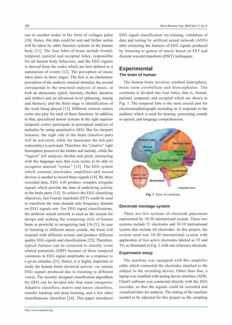
frequency was 2 kHz. In this study, the content of the measured EEG signals (0.5-65 Hz) was band-passed with a cut-off 4th order Butterworth filter which was used with minimum stop band attenuation of 3 dB with ripple in the pass band less than 0.1 dB, and any signal outside the range would be rejected as it was classified as undesired signals. In this experiment, a single channel with three electrodes was used on the interest region of the scalp namely Fpz, T3 and T4. The reference electrode also called as the ground electrode was the Fpz which represented the frontal region, while the two active electrodes were on the temporal lobe region marked by T3 and T4. In order to attach these electrodes, a 10-20 montage system was used as it would indicate the correct placement for the electrodes. A comfy chair needed to be prepared as the subject would be instructed to be seated in their most comfortable manner as the experiment would take a long duration about 22 min. Four different genres of music: Jazz, rock, classical, and heavy metal were used in this project. For each genre, there were four samples of melodies played that formed a total of four trial which comprised the four genres in each trial. Therefore, the number of song sections was 16 and the length of each song section was 60 sec for each genre and 15 sec of rest intervals before a new melody was played. These melodies would be played through an earphone of multi-player device (mp4) that would be plugged to the subjects’ ears. Table 1 shows the display order of the melodies. 30 subjects, male and female, with age ranging from 21 to 24 years old were chosen for the test. Each subject was selected, ensured that

they were in their best condition of health, with no background of neurophysiologic disorder, and with good hearing capability. For male subject, they must not wear any hair gels and needed to ensure their hair was dry. Other than that, the subjects needed to get sufficient break previous to the test being carried out. Throughout the test, the subject would be instructed to sit motionless and comfortably because any movement performed by the subject might interrupt the signal generated later. Apart from that, the subjects were exposed to the same sample of trials for 22 min, and for the analysis, each 60 sec from the different melodies that formed the trial would be used for feature extraction. Fig. 3 indicates the reference and active electrodes on the subject’s scalp.

Frequency domain featuresThe FFT could analyze the frequency components

of a sound. From each frequency achieved, the arithmetical data could be gained for additional investigation and the values that could be measured

Fig. 2 Electrode placement system.

20%

10%

10%NASION

20%

20%

20%

10%INIOH

10% 20% 20%

20%

20%

20%

10%

20%

Fp2FpzFp1

Fz

Pz

F7

T3

T5

O1Oz

O2

T6

T4C4

F4F3

P3 P4

C3Cz

F2

Table 1 Order of melodiesTrial 1 Jazz Rock Classical Heavy metal

Trial 2 Classical Heavy metal Jazz Rock

Trial 3 Heavy metal Jazz Rock Classical

Trial 4 Rock Classical Heavy metal Jazz

Fig. 3 Reference and active electrodes at Fpz, T3 and T4.



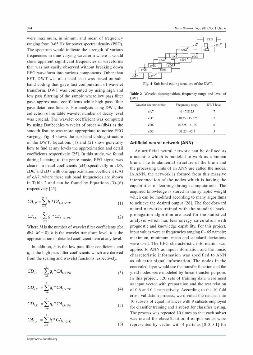
were maximum, minimum, and mean of frequency ranging from 0-65 Hz for power spectral density (PSD). The spectrum would indicate the strength of various frequencies in time varying waveform where it would show apparent significant frequencies in waveforms that was not easily observed without breaking down EEG waveform into various components. Other than FFT, DWT was also used as it was based on sub-band coding that gave fast computation of wavelet transform. DWT was computed by using high and low pass filtering of the sample where low pass filter gave approximate coefficients while high pass filter gave detail coefficients. For analysis using DWT, the collection of suitable wavelet number of decay level was crucial. The wavelet coefficient was computed by using Daubechies wavelet of order 4 (db4) as the smooth feature was more appropriate to notice EEG varying. Fig. 4 shows the sub-band coding structure of the DWT; Equations (1) and (2) show generally how to find at any levels the approximation and detail coefficients respectively [25]. In this study, we found during listening to the genre music, EEG signal was clearer in detail coefficients (cD) specifically in cD5, cD6, and cD7 with one approximation coefficient (cA) of cA7, where these sub band frequencies are shown in Table 2 and can be found by Equations (3)-(6) respectively [25].

1

, 1, 2*0,

*M

b K i b i Ki

CA h CA−

− +=

= ∑ (1)

1

, 1, 2*0

*M

b K i b i Ki

CD g CD−

− +=

= ∑ (2)

Where M is the number of wavelet filter coefficients (for db4, M = 8), b is the wavelet transform level, k is the approximation or detailed coefficient item at any level.

In addition, hi is the low pass filter coefficients and gi is the high pass filter coefficients which are derived from the scaling and wavelet functions respectively.

7

5, 4, 2*0

*K i i Ki

CD g CA +=

=∑ (3)

7

6, 5, 2*0

*K i i Ki

CD g CA +=

=∑ (4)

7

7, 6, 2*0

*K i i Ki

CD g CA +=

=∑ (5)

7

7, 6, 2*0

*K i i Ki

CA h CA +=

=∑ (6)

Artificial neural network (ANN)

An artificial neural network can be defined as a machine which is modeled to work as a human brain. The fundamental structure of the brain and the processing units of an ANN are called the nodes. In ANN, the network is formed from this massive interconnection of the nodes which is having the capabilities of learning through computations. The acquired knowledge is stored in the synaptic weight which can be modified according to many algorithms to achieve the desired output [26]. The feed-forward neural networks trained with the standard back-propagation algorithm are used for the statistical analysis which has less energy calculation with prognostic and knowledge capability. For this project, input values were at frequencies ranging 0 - 65 namely; maximum, minimum, mean and standard deviations were used. The EEG characteristic information was applied to ANN as input information and the music characteristic information was specified to ANN as educator signal information. The nodes in the concealed layer would use the transfer function and the yield nodes were modeled by linear transfer purpose. In this project, 320 sets of training data were used as input vector with preparation and the test relation of 0.6 and 0.4 respectively. According to the 10-fold cross validation process, we divided the dataset into 10 subsets of equal instances with 9 subsets employed for classifier training and 1 subset for classifier testing. The process was repeated 10 times so that each subset was tested for classification. 4 output nodes were represented by vector with 4 parts as [0 0 0 1] for

Fig. 4 Sub-band coding structure of the DWT.

cA7

cA6 cD6

cA4

cA2cA1

cA3cD4

cD2

EEG

cD1

cD3

cA5 cD5

cD7

Table 2 Wavelet decomposition, frequency range and level of DWT

Wavelet decomposition Frequency range DWT level

cA7 0 - 7.8125 7

cD7 7.8125 - 15.625 7

cD6 15.625 - 31.25 6

cD5 31.25 - 62.5 5



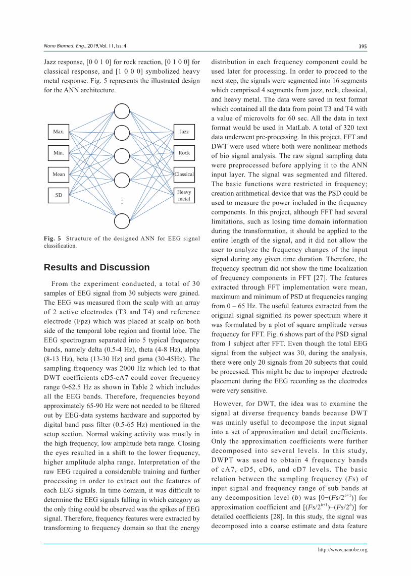
Jazz response, [0 0 1 0] for rock reaction, [0 1 0 0] for classical response, and [1 0 0 0] symbolized heavy metal response. Fig. 5 represents the illustrated design for the ANN architecture.

Results and DiscussionFrom the experiment conducted, a total of 30

samples of EEG signal from 30 subjects were gained. The EEG was measured from the scalp with an array of 2 active electrodes (T3 and T4) and reference electrode (Fpz) which was placed at scalp on both side of the temporal lobe region and frontal lobe. The EEG spectrogram separated into 5 typical frequency bands, namely delta (0.5-4 Hz), theta (4-8 Hz), alpha (8-13 Hz), beta (13-30 Hz) and gama (30-45Hz). The sampling frequency was 2000 Hz which led to that DWT coefficients cD5-cA7 could cover frequency range 0-62.5 Hz as shown in Table 2 which includes all the EEG bands. Therefore, frequencies beyond approximately 65-90 Hz were not needed to be filtered out by EEG-data systems hardware and supported by digital band pass filter (0.5-65 Hz) mentioned in the setup section. Normal waking activity was mostly in the high frequency, low amplitude beta range. Closing the eyes resulted in a shift to the lower frequency, higher amplitude alpha range. Interpretation of the raw EEG required a considerable training and further processing in order to extract out the features of each EEG signals. In time domain, it was difficult to determine the EEG signals falling in which category as the only thing could be observed was the spikes of EEG signal. Therefore, frequency features were extracted by transforming to frequency domain so that the energy

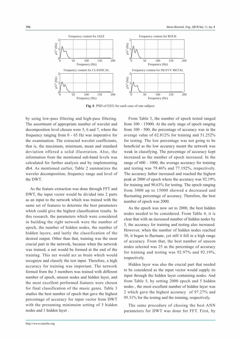
distribution in each frequency component could be used later for processing. In order to proceed to the next step, the signals were segmented into 16 segments which comprised 4 segments from jazz, rock, classical, and heavy metal. The data were saved in text format which contained all the data from point T3 and T4 with a value of microvolts for 60 sec. All the data in text format would be used in MatLab. A total of 320 text data underwent pre-processing. In this project, FFT and DWT were used where both were nonlinear methods of bio signal analysis. The raw signal sampling data were preprocessed before applying it to the ANN input layer. The signal was segmented and filtered. The basic functions were restricted in frequency; creation arithmetical device that was the PSD could be used to measure the power included in the frequency components. In this project, although FFT had several limitations, such as losing time domain information during the transformation, it should be applied to the entire length of the signal, and it did not allow the user to analyze the frequency changes of the input signal during any given time duration. Therefore, the frequency spectrum did not show the time localization of frequency components in FFT [27]. The features extracted through FFT implementation were mean, maximum and minimum of PSD at frequencies ranging from 0 – 65 Hz. The useful features extracted from the original signal signified its power spectrum where it was formulated by a plot of square amplitude versus frequency for FFT. Fig. 6 shows part of the PSD signal from 1 subject after FFT. Even though the total EEG signal from the subject was 30, during the analysis, there were only 20 signals from 20 subjects that could be processed. This might be due to improper electrode placement during the EEG recording as the electrodes were very sensitive.

However, for DWT, the idea was to examine the signal at diverse frequency bands because DWT was mainly useful to decompose the input signal into a set of approximation and detail coefficients. Only the approximation coefficients were further decomposed into several levels. In this study, DWPT was used to obtain 4 frequency bands of cA7, cD5, cD6, and cD7 levels. The basic relation between the sampling frequency (Fs) of input signal and frequency range of sub bands at any decomposition level (b) was [0−(Fs/2b+1)] for approximation coefficient and [(Fs/2b+1)−(Fs/2b)] for detailed coefficients [28]. In this study, the signal was decomposed into a coarse estimate and data feature

Fig. 5 Structure of the designed ANN for EEG signal classification.

Max.

Min.

Mean

SD

Jazz

Rock

Classical

Heavymetal



by using low-pass filtering and high-pass filtering. The assortment of appropriate number of wavelet and decomposition level chosen were 5, 6 and 7, where the frequency ranging from 0 - 65 Hz was imperative for the examination. The extracted wavelet coefficients, that is, the maximum, minimum, mean and standard deviation offered a solid illustration. Also, the information from the mentioned sub-band levels was calculated for further analysis and by implementing db4. As mentioned earlier, Table 2 summarizes the wavelet decomposition, frequency range and level of the DWT.

As the feature extraction was done through FFT and DWT, the input vector would be divided into 2 parts as an input to the network which was trained with the same set of features to determie the best parameters which could give the highest classification results. In this research, the parameters which were considered in building the right network were the number of epoch, the number of hidden nodes, the number of hidden layers, and lastly the classification of the desired output. Other than that, training was the most crucial part in the netwrok, because when the netwrok was trained, a net would be formed at the end of the training. This net would act as brain which would recognize and classify the test input. Therefore, a high accuracy for training was important. The network formed from the 3 members was trained with different number of epoch, unseen nodes and hidden layer, and the most excellent performed features were chosen for final classification of the music genre. Table 3 studies the best number of epoch that gave the highest percentage of accuracy for input vector from DWT with the presuming minimuim setting of 5 hidden nodes and 1 hidden layer .

From Table 3, the number of epoch tested ranged from 100 - 15000. At the early stage of epoch ranging from 100 - 500, the percentage of accuracy was in the average value of 62.812% for training and 51.252% for testing. The low percentage was not going to be beneficial as the low accuracy meant the network was weak in classifying. The percentage of accuracy kept increased as the number of epoch increased. In the range of 600 - 1000, the average accuracy for training and testing was 79.46% and 77.192%, respectively. The accuracy futher increased and reached the highest peak at 2000 of epoch where the accuracy was 92.19% for training and 90.63% for testing. The epoch ranging from 3000 up to 15000 showed a decreased and fluctuating percentage of accuracy. Therefore, the best number of epoch was 2000.

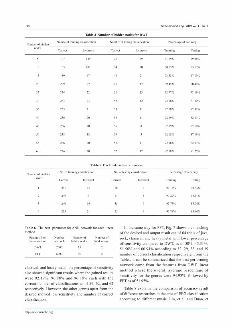
As the epoch was now set to 2000, the best hidden nodes needed to be considered. From Table 4, it is clear that with an increased number of hidden nodes by 5, the accuracy for training and testing also increased. However, when the number of hidden nodes reached 30, it began to fluctuate, yet still it fell in a high range of accuracy. From that, the best number of unseen nodes selected was 25 as the percentage of accuracy for training and testing was 92.97% and 92.19%, respectively.

Hidden layer was also the crucial part that needed to be considered as the input vector would supply its input through the hidden layer containing nodes. And from Table 5, by setting 2000 epoch and 5 hidden nodes , the most excellent number of hidden layer was 2 which gave the highest accuracy of 97.27% and 95.31% for the testing and the training, respectively.

The same procedure of chosing the best ANN parameters for DWT was done for FFT. First, by

Fig. 6 PSD of EEG for each case of one subject.

2

1

00 50 100

Frequency (Hz)150 200

Frequency content for JAZZ

µV2 (

Hz)

2

1

00 50 100


Frequency content for ROCK

µV2 (

Hz)

2

1

00 50 100


Frequency content for CLASSICAL

µV2 (

Hz)

2

1

00 50 100


Frequency content for HEAVY METAL

µV2 (

Hz)



setting 5 hidden nodes, 1 hidden layer, we found that the best number of epoch was 6000 which gave the highest accuracy of 71.34% and 26.56% for training and testing respectively. Second, by setting 6000 epoch, 1 hidden layer, we found that 35 hidden nodes gave the highest accuracy of 73.24% and 27.81% for training and testing respectively. Finally, in order to chosse the best hidden layer, we set 6000 epoch, 35 hidden nodes to give 96.48% and 31.00% for training and testing respectively with 2 hidden layers. It is clear that FFT features produced lower percentage of accuracy for training and testing compared to the DWT features.

Table 6 summarizes the suitable number of epoch, hidden nodes and hiden layer for features from DWT and FFT. It is very clear that FFT features took longer time than DWT because of using more hidden nodes

with very long number of epoch. Generally speaking, execution time of the former method was half of the later one in our case of study.

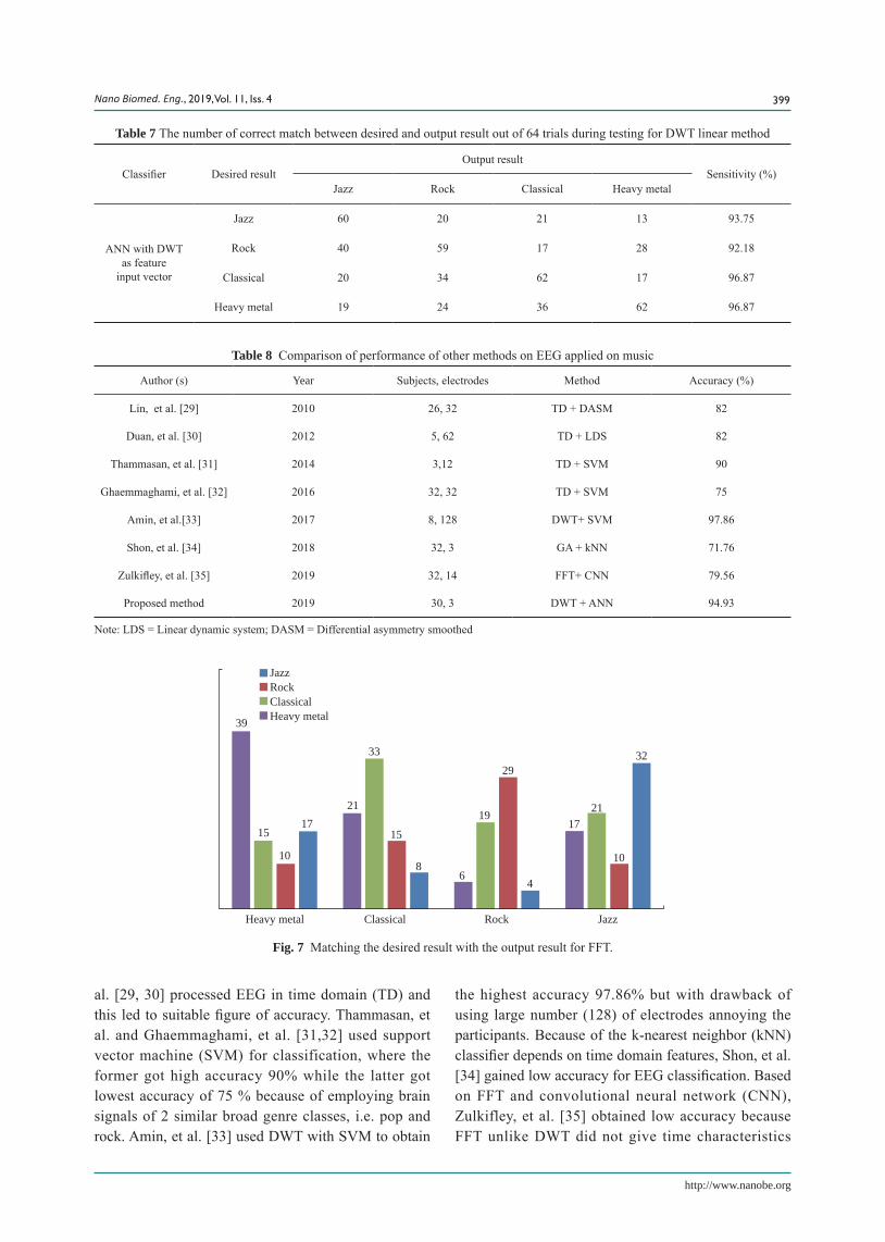
Right after the correct network was established for input vector from DWT linear method, the testing was performed. Table 7 shows how often the desired result matched the output result through expressing the network performance by its sensitivity in Equation (7).

Sensitivity% = [True positive/(True positive +False negative)] × 100 (7)

For example, the desired jazz result gave the value of sensitivity for testing as of 93.75% with 60 correct classifications out of 64, with the remaining undesired genres being low in sensitivity as of 31.25%, 32.81% and 20.31% for rock, classical, and heavy metal respectively. When the desired result was rock,

Table 3 DWT epoch numbers

Number of epochNo. of training classification No. of testing classification Percentage of accuracy

Correct Incorrect Correct Incorrect Training Testing

100 144 112 27 37 56.25% 42.19%

200 160 96 33 31 62.50% 51.56%

300 161 95 30 34 62.89% 46.88%

400 164 92 32 32 64.06% 50.00%

500 175 81 42 20 68.36% 65.63%

600 200 56 49 15 78.13% 76.56%

700 201 55 47 17 78.52% 73.45%

800 203 53 50 14 79.30% 78.13%

900 205 51 50 14 80.10% 78.13%

1000 208 48 51 13 81.25% 79.69%

2000 236 20 58 6 92.19% 90.63%

3000 212 44 52 12 82.81% 81.25%

4000 220 36 53 11 85.94% 82.81%

5000 227 29 51 13 88.67% 79.69%

6000 225 31 56 8 87.89% 87.50%

7000 231 25 55 9 90.23% 85.94%

8000 232 24 56 8 90.63% 87.50%

9000 235 21 58 6 91.80% 90.63%

10000 235 21 57 7 91.80% 89.06%

15000 235 21 55 9 91.80% 85.94%



classical, and heavy metal, the percentage of sensitivity also showed significant results where the gained results were 92.19%, 96.88% and 96.88% each with the correct number of classifications as of 59, 62, and 62 respectively. However, the other genres apart from the desired showed low sensitivity and number of correct classification.

In the same way for FFT, Fig. 7 shows the matching of the desired and output result out of 64 trials of jazz, rock, classical, and heavy metal with lower percentage of sensitivity compared to DWT, as of 50%, 45.31%, 51.56% and 60.94% according to 32, 29, 33, and 39 number of correct classification respectively. From the Tables, it can be summarized that the best performing network came from the features from DWT linear method where the overall average percentage of sensitivity for the genres were 94.93%, followed by FFT as of 51.95%.

Table 8 explains the comparison of accuracy result of different researches in the area of EEG classification according to different music. Lin, et al. and Duan, et

Table 4 Number of hidden nodes for DWT

Number of hidden nodes

Numbe of training classification Number of testing classification Percentage of accuracy


5 107 149 25 39 41.79% 39.06%

10 155 101 34 30 60.55% 53.13%

15 189 67 43 21 73.83% 67.19%

20 229 27 47 17 89.45% 80.44%

25 234 22 51 13 92.97% 92.19%

30 233 23 52 12 92.18% 81.80%

35 235 21 53 11 92.18% 82.81%

40 236 20 53 11 92.19% 82.81%

45 236 20 56 8 92.19% 87.50%

50 238 18 59 5 92.18% 87.19%

55 236 20 53 11 92.18% 82.81%

60 236 20 52 12 92.18% 81.25%

Table 5 DWT hidden layers numbers

Number of hiddden layer

No. of training classification No. of testing classification Percentage of accuracy


1 241 15 58 6 91.14% 90.63%

2 249 7 61 3 97.27% 95.31%

3 240 16 55 9 93.75% 85.94%

4 235 21 55 9 91.78% 85.94%

Table 6 The best parameter for ANN network for each linear method

Features fromlinear method

Numberof epoch

Number ofhidden nodes

Number ofhidden layer

DWT 2000 25 2

FFT 6000 35 2



al. [29, 30] processed EEG in time domain (TD) and this led to suitable figure of accuracy. Thammasan, et al. and Ghaemmaghami, et al. [31,32] used support vector machine (SVM) for classification, where the former got high accuracy 90% while the latter got lowest accuracy of 75 % because of employing brain signals of 2 similar broad genre classes, i.e. pop and rock. Amin, et al. [33] used DWT with SVM to obtain

the highest accuracy 97.86% but with drawback of using large number (128) of electrodes annoying the participants. Because of the k-nearest neighbor (kNN) classifier depends on time domain features, Shon, et al. [34] gained low accuracy for EEG classification. Based on FFT and convolutional neural network (CNN), Zulkifley, et al. [35] obtained low accuracy because FFT unlike DWT did not give time characteristics

Table 7 The number of correct match between desired and output result out of 64 trials during testing for DWT linear method

Classifier Desired resultOutput result

Sensitivity (%)Jazz Rock Classical Heavy metal

ANN with DWTas feature

input vector

Jazz 60 20 21 13 93.75

Rock 40 59 17 28 92.18

Classical 20 34 62 17 96.87

Heavy metal 19 24 36 62 96.87

Table 8 Comparison of performance of other methods on EEG applied on music

Author (s) Year Subjects, electrodes Method Accuracy (%)

Lin, et al. [29] 2010 26, 32 TD + DASM 82

Duan, et al. [30] 2012 5, 62 TD + LDS 82

Thammasan, et al. [31] 2014 3,12 TD + SVM 90

Ghaemmaghami, et al. [32] 2016 32, 32 TD + SVM 75

Amin, et al.[33] 2017 8, 128 DWT+ SVM 97.86

Shon, et al. [34] 2018 32, 3 GA + kNN 71.76

Zulkifley, et al. [35] 2019 32, 14 FFT+ CNN 79.56

Proposed method 2019 30, 3 DWT + ANN 94.93

Note: LDS = Linear dynamic system; DASM = Differential asymmetry smoothed

Fig. 7 Matching the desired result with the output result for FFT.

Heavy metal Classical Rock Jazz

JazzRockClassicalHeavy metal39

15

10

1721

33

15

86

19

29

4

1721

10

32



of the genre class. Unlike the previous methods, the proposed method depended on frequency domain to extract the EEG features by using DWT which gave 94.93% depending on the ANN best parameters chosen after different tests with expected higher accuracy by using SVM in future work.

As application of techniques in this study, we can apply sort of music on patient to notice the relation between his feeling and the EEG rhythm especially for handicapped patient as some common music therapy practices include developmental work (communication, motor skills, etc.) with individuals special needs and rhythmic entrainment for physical rehabilitation in stroke victims.

ConclusionsThe EEG signals were collected from 30 subject

having a good condition of health; however for the analysis, only 20 subjects were considered as the data collected, given that the remaining 10 subject could not be used for futher processing due to incorrect procedure during recording. As the raw signal was in time domain, it was not possible to straight-away feed it to the ANN. Therefore, a step was taken by implementing a linear method which operated in changing the time domain signal to frequency domain. The linear method was done by applying DWT and the FFT. From the linear method, several features were extrected out. For DWT, the greatest, smallest, signified and normal deviations were used for the aspect and estimated coefficient, while for FFT, the maximum, minimum and mean were taken through PSD. In this project, the ANN was used for the classification purpose. The neural network was skilled using feedfoward network with back-propagation algorithm. The network form could be divided into individual network which consisted of features from DWT and FFT. It was observed that DWT got the highest acuracy in classifying. Finally, the used technique succesfully classified the EEG signals of jazz, rock, classical, and heavy metal. EEG signal is a complex system to be discovered where it gives a wide area of research. The approach of ANN can improve the classification accuracy. ANN is not only the existing classifier as there are so many other classifiers that can be tried out for future classification and be implemented in this area. For example the adaptive network-based fuzzy inference system (ANFIS) and fuzzy classifier that might give a higher accuracy compared to ANN.

Conflict of Interests

The authors declare that no competing interest exists.

References

[1] M. Soegaard, R.F. Dam, Human computer interaction- brief intro. The encyclopedia of human-computer interaction , 2nd edition. The Intetraction Design Foundation, 2012: page number.

[2] M.Z. Baig, N. Aslam, H.P.H. Shum, et al., Differential evolution algorithm as a tool for optimal feature subset selection in motor imagery EEG. Expert Syst. Appl., 2017, 90: 184-195.

[3] V.P. Oikonomou, K. Georgiadis, G. Liaros, et al., A comparison study on EEG signal processing techniques using motor imagery EEG data. Proceedings of the IEEE 30th International Symposium on Computer-Based Medical Systems (CBMS). Thessaloniki, Greece, Jun. 22-24, 2017.

[4] D. Cheng, Y, Liu, and L. Zhang, Exploring motor imagery EEG patterns for stroke patients with deep neural networks. Proceedings of the IEEE International Conference on Acoustics, Speech and Signal Processing (ICASSP). Calgary, AB, Canada, Apr. 15-20, 2018.

[5] S. Kumar, R, Sharma, A, Sharma, et al., Decimation filter with common spatial pattern and fishers discriminant analysis for motor imagery classification. Proceedings of the International Joint Conference on Neural Networks (IJCNN). Vancouver, BC, Canada, Jul., 24-29, 2016.

[6] X. Guo, X. Wu, X Gong, et al., Envelope detection based on online ICA algorithm and its application to motor imagery classification. Proceedings of the 6th International IEEE/EMBS Conference on Neural Engineering (NER). San Diego, CA, USA, Nov. 6-8, 2013.

[7] A. Nijholt, The future of brain-computer interfacing (keynote paper). Proceedings of the 5th International Conference on Informatics, Electronics and Vision (ICIEV). Dhaka, Bangladesh, May 13-14, 2016.

[8] J, Kevric, A. Subasi, Comparison of signal decomposition methods in classification of EEG signals for motor-imagery BCI system. Biomed. Signal Process. Control, 2017, 31: 398-406.

[9] K. Suefusa, T. Tanaka, A comparison study of visually stimulated brain-computer and eye-tracking interfaces. J. Neural Eng., 2017, 14: 036009.

[10] Y, Zhang, Y. Wang, J. Jin, et al., Sparse Bayesian learning for obtaining sparsity of EEG frequency bands based feature vectors in motor imagery classification. Int. J. Neural Syst., 2017, 27: 1650032.

[11] M.Z. Ilyas, P, Saad, M.I. Ahmad, et al., Classification of EEG signals for brain-computer interface applications: Performance comparison. Proceedings of the 6th International IEEE/EMBS Conference on Neural Engineering (NER). Ayer Keroh, Malaysia, Nov. 5-6, 2016.

[12] D. Gajic, Z. Djurovic, S.D. Gennaro, et al., Classification of EEG signals for detection of epileptic seizures based on wavelets and statistical pattern recognition. Biomed. Eng., 2014, 26: 1450021.

[13] A. Montinaro, The musical brain: Myth and science. World Neurosurgery, 2010, 73(5): 442-453.

[14] R.T. Schirrmeister, J.T. Springenberg, L.D.J. Fiederer, et al., Deep learning with convolutional neural networks for EEG decoding and visualization. Hum. Brain Mapp., 2017, 38: 5391-5420.



[15] Z. Tang, C. Li, S. Sun, Single-trial EEG classification of motor imagery using deep convolutional neural networks. Optik, 2017, 130: 11-18.

[16] Y. Tabar, U. Halici, A novel deep learning approach for classification of EEG motor imagery signals. J. Neural Eng., 2017, 14: 016003.

[17] P. Batres-Mendoza, C. Montoro-Sanjose, E. Guerra-Hernandez, et al., Quaternion-based signal analysis for motor imagery class i f icat ion from electro-encephalographic signals. Sensors, 2016, 16: 336

[18] A. Liu, K. Chen, Q. Liu, et al., Feature selection for motor imagery EEG classification based on firefly algorithm and learning automata. Sensors, 2017, 17: 2576

[19] Y. Wang, X. Li, H. Li, et al., Feature extraction of motor imagery electroencephalography based on time-frequency-space domains. J. Biomed. Eng. 2014, 31: 955-961.

[20] T.T. Day, Applying a locally linear embedding algorithm for feature extraction and visualization of MI-EEG. J. Sens., 2016: 7481946.

[21] R. Zazo, A. Lozano-Diez, J. Gonzalez-Dominguez, et al., Language identification in short utterances using long short-term memory (LSTM) recurrent neural networks. PLoS ONE, 2016, 11: e0146917.

[22] M. Li, W. Chen, and T. Zhang, Classification of epilepsy EEG signals using DWT-based envelope analysis and neural network ensemble. Biomed. Signal Process. Control, 2017, 31: 357-365.

[23] F. Lotte, A tutorial on EEG signal-processing techniques for mental-state recognition in brain computer interfaces. Guide to brain-computer music interfacing. Springer, 2014: 133-161.

[24] F. Lotte, L. Bougrain, A. Cichocki , et al., A review of classification algorithms for EEG-based brain-computer interfaces: A 10-year update. Journal of Neural Engineering, 2018, 15(3): 55.

[25] M. Wali, M. Murugappan, and B. Ahmmad, Wavelet packet t ransform based driver distract ion level classif icat ion using EEG, Hindawi Publishing Corporation, Mathematical Problems in Engineering, 2013: Article ID 297587.

[26] M.B. Kurt, N. Sezgin, M. Akin, et al., The ANN-based computing of drowsy level. Expert Systems with Applications, 2009, 36(2): 2534-2542.

[27] M. Sifuzzaman, M. Islam, and M. Ali, Application of wavelet transform and its advantages compared to Fourier transform. Journal of Physical Sciences, 2009, 13: 121-134.

[28] M. Wali, M. Murugappan, and B. Ahmmad, Mathematical implementation of hybrid FFT and DWT for developing graphical user interface using visual basic for signal processing applications. Journal of Mechanics in Medicine and Biology, 2012, 12(5): 1240031.

[29] Y. Lin, C. Wang, T. Jung, et al., EEG-based emotion recognition in music listening. IEEE Trans. on Biomedical Engineering, 2010, 57(7): 1798-1806.

[30] R. Duan X. Wang, and B. Lu, EEG-based Emotion Recognition in listening music by using support vector machine and linear dynamic system. Proceedings of the 19th International Conference on Neural Information. 2012: 468-475.

[31] N. Thammasan, K. Fukui, K. Moriyama,, et al., EEG-based emotion recognition during music listening. Proceedings of the 28th Conference of the Japanese Society of Artificial Intelligence. 2014.

[32] P. Ghaemmaghami, N Sebe, Brain and music: Music genre classification using brain signals. Proceedings of the 24th International Conference on Signal Processing (EUSIPCO). 2016: 708-712.

[33] H.U. Amin, W. Mumtaz , A.R. Subhani , e t a l . , Classification of EEG signals based on pattern recognition approach. Frontiers in Computational Neuroscience, 2017.

[34] D. Shon, K. Im, J. Park, et al., Emotional stress state detection using genetic algorithm-based feature selection on EEG signals. Int. J. Environ. Res. Public Health, 2018, 15: 2461.

[35] M. Zulkifley, S. Abdani, EEG signals classification by using convolutional neural networks. SASSP, 2019.

Copyright© Mousa Kadhim Wali. This is an open-access article distributed under the terms of the Creative Commons Attribution License, which permits unrestricted use, distribution, and reproduction in any medium, provided the original author and source are credited.

Documents

Nano Biome. n. N ano B iomed Eng - nanobe.org