Embed Size (px)
DESCRIPTION
By Ertan Gul, Baris Atakan, Ozgur B. Akan
Citation preview
Nano Communication Networks 1 (2010) 138–156
Contents lists available at ScienceDirect
Nano Communication Networks
journal homepage: www.elsevier.com/locate/nanocomnet
NanoNS: A nanoscale network simulator framework for molecularcommunicationsErtan Gul, Baris Atakan, Ozgur B. Akan ∗Next-generation Wireless Communications Laboratory, Department of Electrical and Electronics Engineering, Koc University, 34450, Istanbul, Turkey
a r t i c l e i n f o
Article history:Received 30 July 2010Accepted 5 August 2010Available online 22 August 2010
Keywords:Molecular communicationMolecular diffusionNanonetworksNanonetwork simulation toolNS-2
a b s t r a c t
A number of nanomachines that cooperatively communicate and share molecular infor-mation in order to achieve specific tasks is envisioned as a nanonetwork. Due to the sizeand capabilities of nanomachines, the traditional communication paradigms cannot beused for nanonetworks in which network nodes may be composed of just several atomsor molecules and scale on the orders of few nanometers. Instead, molecular commu-nication is a promising solution approach for the nanoscale communication paradigm.However, molecular communication must be thoroughly investigated to realize nanoscalecommunication and nanonetworks for many envisioned applications such as nanoscalebody area networks, and nanoscalemolecular computers. In this paper, a simulation frame-work (NanoNS) formolecular nanonetworks is presented. The objective of the framework isto provide a simulation tool in order to create a better understanding of nanonetworks andfacilitate the development of new communication techniques and the validation of theo-retical results. The NanoNS framework is built on top of core components of a widely usednetwork simulator (ns-2). It incorporates the simulation modules for various nanoscalecommunication paradigms based on a diffusivemolecular communication channel. The de-tails ofNanoNS are discussed and some functional scenarios are defined to validateNanoNS.In addition to this, the numerical analyses of these functional scenarios and their experi-mental results are presented. The validation of NanoNS is shown via comparative evalua-tion of these experimental and numerical results.
© 2010 Elsevier Ltd. All rights reserved.
1. Introduction
Nanotechnology enables the practical realization ofnanoscale devices commonly referred to as nanomachines,the size of which ranges from 1 to 100 nm. The fabricationtechniques in nanotechnology can be categorized into twomain groups, i.e., dry and wet techniques. Dry techniquesare mostly used for the fabrication of carbon nanotubesand nanowires whereas wet techniques are employed tofabricate nanoscale biological systems that already exist innatural aqueous media.The realization of such biological nanomachines has
been always worked by a large set of biochemical methods
∗ Corresponding author.E-mail address: [email protected] (O.B. Akan).
1878-7789/$ – see front matter© 2010 Elsevier Ltd. All rights reserved.doi:10.1016/j.nancom.2010.08.003
for many years. For example, biochemists already tacklewith the production of functional cell components suchas ribosomes that can be programmed for the synthesisof beneficial proteins. Doubtlessly, a network of commu-nicating nanomachines can also be programmed to sharenanoscale information over a nanonetwork so as to fulfillmore complex tasks such as collaborative drug delivery,healthmonitoring, and biological or chemical attack detec-tion [5].In the literature, there are currently fourmainnanoscale
communication techniques, i.e., nanomechanical, acoustic,molecular, and electromagnetic communication that maybe used for the realization of nanonetworks [12]. In acous-tic communication, information is carried via an acous-tic signal. In nanomechanical communication, informationflows through the mechanical connection of nanoscale de-vices. In electromagnetic communication, information is
E. Gul et al. / Nano Communication Networks 1 (2010) 138–156 139
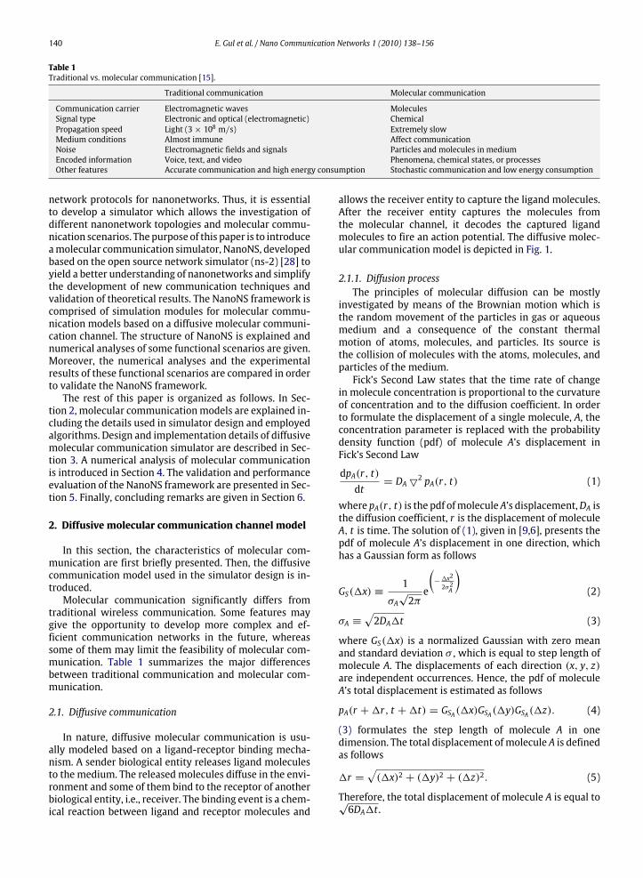
TN RN
DIFFUSIVE MOLECULAR CHANNEL
Receptor
Ligand (Molecule)
Fig. 1. Diffusive molecular communication model [2].
encoded into electromagnetic waves [4]. Molecular com-munication provides nanoscale communication amongnanomachines using molecules as communication carri-ers [1].Due to lack of the acoustic, nanomechanical, and eletro-
magnetic communication hardware that are sufficientlysmall and biologically compatible, molecular communi-cation is the most promising and biologically compati-ble communication paradigm in order to enable frontiernanonetworks. Molecular communication can be viewedas an interdisciplinary research area that incorporates thedomain of nanotechnology, biotechnology, and communi-cation theory. Thus, the performance ofmolecular commu-nication systems is affected by the physical laws in thesedomains. This brings many crucial research challenges,thatmust be efficiently addressed, into traditional commu-nication systems.Molecular communication systems can be categorized
into three main groups according to their propagationmechanisms, i.e., diffusive, motor-based and gap junction-based molecular communication. Molecular communica-tion through gap junctions, inspired from inter-cellularcommunication in nature, is presented in [23]. The system,in which calcium signaling is used as a communicationcarrier, is based on the diffusion of information moleculesthrough gap junctions connecting the cytoplasmof two ad-jacent cells. The permeability and selectivity of gap junc-tions vary according to the constructive proteins of the gapjunction [10]. In [22], the detailed design of a molecularchannel with gap junctions is proposed. Signal switching,filtering and aggregation functionalities are controlled byadjusting the permeability and selectivity of gap junctions.Molecular motor-based communication is inspired
from intra-cell communication of real biological cells.Message molecules are transported by molecular motorsand protein filaments that naturally exist in biomolecu-lar linear systems [27]. There are two propagation typesin molecular motor-based communication systems. In[21,20], carrier molecules are inserted into a vesicle em-bedded with channel proteins to transport the molecules.Vesicles, which encapsulate the information molecules,behave like communication interfaces between sender andreceiver. They protect carriermolecules from environmen-tal conditions and maintain compatibility between infor-mation molecules and environment.In addition to gap junction-based and motor-based
communications, molecules may also freely propagate
in an aqueous medium to allow the diffusive molecularcommunication among nanomachines. Diffusive molecu-lar communication is one of the fundamental communica-tion mechanisms that is used by biological systems. Thismodel is based on passive transport, which means that noexternal energy is required during transportation. In thismodel, the transmitter nanomachine releases moleculesinto an aqueous medium, then molecules propagate in themedium, and the receiver nanomachine captures some ofthese molecules that chemically react with its receptors asin Fig. 1. A simplified version of the ligand-receptor mech-anism is analyzed and the channel capacity of the diffusivebiochemical channel is estimated in [29]. A physicalmolec-ular channel is modeled and analyzed in [25]. Moreover,an information theoretical approach for molecular com-munication is presented in [2], where the molecular com-munication channel capacity between two nanomachinesis analyzed. Molecular multiple access, broadcast and re-lay channel models for molecular communication are pre-sented, and their capacity expressions are derived in [3].In the current literature, the methodologies and tools
used to analyze molecular communication and investigateits performance are extremely limited. In [17], unicastcommunication on microtubule topology is investigated.The probability of successful transmission is comparedfor the cases of diffusive and motor-based propagation.However, the topology of the environment is composedof only one single sender, one single receiver and themicrotubule, which renders the nanonetwork topologyoversimplified andunrealistic. In [16], delay characteristicsof different microtubule topologies are analyzed. In [18],three types of molecular communication propagationapproaches are defined. In a diffusive propagation system,microtubules are not used to connect sender and receiver.In a motor-based propagation system, sender and receiverare connected and an information molecule is directlytransferred from the sender to the receiver nanomachine.In the hybrid propagation system, information moleculesare released, then information molecules may propagateto the receiver by diffusing in the environment or bindingmicrotubule which has an unstable behavior and movesthrough the bound microtubule. The information rates ofpropagation models are compared. Additionally, the noiseanalysis of these models is investigated in [19].Despite promising progress performed in molecular
communication, there is currently no molecular commu-nication simulator which provides a practical and bene-ficial simulation suite to be used in the development of
140 E. Gul et al. / Nano Communication Networks 1 (2010) 138–156
Table 1Traditional vs. molecular communication [15].
Traditional communication Molecular communication
Communication carrier Electromagnetic waves MoleculesSignal type Electronic and optical (electromagnetic) ChemicalPropagation speed Light (3× 10⁸ m/s) Extremely slowMedium conditions Almost immune Affect communicationNoise Electromagnetic fields and signals Particles and molecules in mediumEncoded information Voice, text, and video Phenomena, chemical states, or processesOther features Accurate communication and high energy consumption Stochastic communication and low energy consumption
network protocols for nanonetworks. Thus, it is essentialto develop a simulator which allows the investigation ofdifferent nanonetwork topologies and molecular commu-nication scenarios. The purpose of this paper is to introduceamolecular communication simulator, NanoNS, developedbased on the open source network simulator (ns-2) [28] toyield a better understanding of nanonetworks and simplifythe development of new communication techniques andvalidation of theoretical results. The NanoNS framework iscomprised of simulation modules for molecular commu-nication models based on a diffusive molecular communi-cation channel. The structure of NanoNS is explained andnumerical analyses of some functional scenarios are given.Moreover, the numerical analyses and the experimentalresults of these functional scenarios are compared in orderto validate the NanoNS framework.The rest of this paper is organized as follows. In Sec-
tion 2, molecular communicationmodels are explained in-cluding the details used in simulator design and employedalgorithms. Design and implementation details of diffusivemolecular communication simulator are described in Sec-tion 3. A numerical analysis of molecular communicationis introduced in Section 4. The validation and performanceevaluation of the NanoNS framework are presented in Sec-tion 5. Finally, concluding remarks are given in Section 6.
2. Diffusive molecular communication channel model
In this section, the characteristics of molecular com-munication are first briefly presented. Then, the diffusivecommunication model used in the simulator design is in-troduced.Molecular communication significantly differs from
traditional wireless communication. Some features maygive the opportunity to develop more complex and ef-ficient communication networks in the future, whereassome of them may limit the feasibility of molecular com-munication. Table 1 summarizes the major differencesbetween traditional communication and molecular com-munication.
2.1. Diffusive communication
In nature, diffusive molecular communication is usu-ally modeled based on a ligand-receptor binding mecha-nism. A sender biological entity releases ligand moleculesto the medium. The released molecules diffuse in the envi-ronment and some of them bind to the receptor of anotherbiological entity, i.e., receiver. The binding event is a chem-ical reaction between ligand and receptor molecules and
allows the receiver entity to capture the ligand molecules.After the receiver entity captures the molecules fromthe molecular channel, it decodes the captured ligandmolecules to fire an action potential. The diffusive molec-ular communication model is depicted in Fig. 1.
2.1.1. Diffusion processThe principles of molecular diffusion can be mostly
investigated by means of the Brownian motion which isthe random movement of the particles in gas or aqueousmedium and a consequence of the constant thermalmotion of atoms, molecules, and particles. Its source isthe collision of molecules with the atoms, molecules, andparticles of the medium.Fick’s Second Law states that the time rate of change
in molecule concentration is proportional to the curvatureof concentration and to the diffusion coefficient. In orderto formulate the displacement of a single molecule, A, theconcentration parameter is replaced with the probabilitydensity function (pdf) of molecule A’s displacement inFick’s Second Law
dpA(r, t)dt
= DA52 pA(r, t) (1)
where pA(r, t) is the pdf ofmoleculeA’s displacement,DA isthe diffusion coefficient, r is the displacement of moleculeA, t is time. The solution of (1), given in [9,6], presents thepdf of molecule A’s displacement in one direction, whichhas a Gaussian form as follows
GS(1x) ≡1
σA√2πe
(−1x2
2σ2A
)(2)
σA ≡√2DA1t (3)
where GS(1x) is a normalized Gaussian with zero meanand standard deviation σ , which is equal to step length ofmolecule A. The displacements of each direction (x, y, z)are independent occurrences. Hence, the pdf of moleculeA’s total displacement is estimated as follows
pA(r +1r, t +1t) = GSA(1x)GSA(1y)GSA(1z). (4)
(3) formulates the step length of molecule A in onedimension. The total displacement ofmolecule A is definedas follows
1r =√(1x)2 + (1y)2 + (1z)2. (5)
Therefore, the total displacement of molecule A is equal to√6DA1t .
E. Gul et al. / Nano Communication Networks 1 (2010) 138–156 141
2.1.2. Reaction processThere are two types of reaction modeling approaches:
a deterministic approach and a stochastic approach. A de-terministic process assumes that the molecular reactionsare continuous and completely predictable processes andmodeled by deterministic differential reaction-rate equa-tions. However, a reaction system is not a continuous pro-cess as the number of molecules changes discretely, andit is not possible to predict the exact molecular populationlevelswithout knowing and tracking the exact position andvelocity of the molecules.Here, in order to devise a realistic channel model in
molecular communication, we follow a stochastic methodcommonly known asGillespie’smethod and introduced fordescribing the stochastic simulation of coupled chemicalreactions in a well-mixed medium [13].In Gillespie’s method, N kinds of molecules which are
able to react with each other throughM reaction channelsare assumed to be uniformly mixed in a fixed volume V .These M reactions are formulated as follows:
R1: S1 + S2 → C1...
RM : SN−1 + SN → CM
M Reaction channels (6)
where Si, i ∈ {1, . . . ,M} are the molecules that react witheach other, Ci, i ∈ {1, . . . ,M} is the output of the Rithreaction channel.In order to determine which reaction occurs next and
when it occurs, P(τ , µ), is defined as the probability thatgiven the state Xi(t) (i = 1, . . . ,N), which denotes thenumber of molecules of the species, at the time t , thenext reaction in the volume will occur in the infinitesimaltime interval (t + τ ; t + τ + dτ) and will be an Rµ.The reaction probability of Rµ is the case that no reactionwill occur during τ after reaction µ has occurred. Hence,P(τ , µ) equals the product of P0(τ ) and the propensityvalue of Rµ, aµ, which gives the probability of occurrenceof reaction µ in (t, t + τ) [13], i.e.,
P(τ , µ)dτ = P0(τ )aµdτ . (7)
The propensity function has a specific mathematical formgiven as
aµ = hµcµ (8)
where cµ is the rate constant which depends on the radiusof the molecules, their average velocities and individualmasses. hµ is the quantity of reaction input combinations.For instance,hµ value of reaction ‘‘Rµ: S1+S2 → anything’’equals X1X2.After applying derivations in [13], P0(τ ) is obtained as
P0(τ ) = e
(−
M∑µ=1
aµτ
). (9)
Substituting (9) into (7) yields
P(τR, µ) =
aµe(−a0τR), 0 ≤ τR <∞,
µ = 1, . . . ,M,0, otherwise
(10)
where aµ = hµcµ and a0 =∑M
υ=1 aυ . As shown in(10), P(τR, µ) is equal to themultiplication of two separatefunctions, f (µ) and g(τ ). τ and µ can be obtained using
τ =1a0ln1r1
(11)
µ−1∑υ=1
aυ < r2a0 ≤µ∑υ=1
aυ (12)
by assigning two random variables, r1, r2, in interval [0, 1][13].
2.1.3. Reaction-diffusion modelThere are several stochastic approaches to model
biochemical activities. We consider a mesoscopic levelarchetype, which treats molecules discretely, however, itdoes not track positions in a compartment or within a sub-volume, to model a molecular channel of the simulator.Since our channel model needs both reaction and diffu-sion capabilities, we model our channel to develop with areaction-diffusion paradigm.In this model, diffusion and reaction are distinct events.
The basis of diffusion is the multiparticle lattice gas au-tomata (LGA) algorithm [26]. In the multiparticle LGAalgorithm, the medium is divided into lattice sides. Con-sequently, the inhomogeneity of the system is reducedto the lattice volume. Each lattice site holds a discretenumber of uniformly distributed particles. Molecules per-form randomwalks on the lattices and are distributed to 6neighbor lattices randomly. If a small number of moleculesexist in the lattice, molecules move individually to neigh-bor lattices. If the number of molecules is larger than60 [26], molecules move in bulk to a lattice according to aGaussian distribution. In the algorithm, the exact positionof amolecule is not necessary, however, only the lattice po-sition of the molecule is required. Thus, lattice coordinatesystem is utilized in the simulator.Normally, every species has a particular diffusion coef-
ficient. The diffusion time step, τDS , of each species is cal-culated as follows
τDS =12dλ2
DS(13)
where DS is diffusion coefficient of the species, λ is thelength of each lattice, d is the dimension of the simulationmedium.As indicated, a reaction process is distinct from a dif-
fusion process. Reaction events occur between diffusionevents. It is assumed that chemical reactions are localevents. Therefore, the Stochastic Simulation Algorithm(SSA) is applied to perform reaction events in each lat-tice side. As mentioned in Section 2.1.2, SSA can only beapplied to well-mixed volumes. Hence, the length of thelattice sides should not be long in order to keep homoge-nization of lattice volume.1 In NanoNS, the lattice lengthis a user-defined input parameter. If the length of lattice
1 The analysis of the optimal lattice size is beyond the scope of thiswork. An analysis of optimal lattice size is presented in [26].
142 E. Gul et al. / Nano Communication Networks 1 (2010) 138–156
TclCLSimulation
ObjectsSimulation
Objects
C++
ns-2 Tcl Interpreter Shell (ns)
Tcl Simulation
ScriptSimulationTrace File
NamAnimation
Analysis
Graphplotting
NS Simulator Library
OTcl
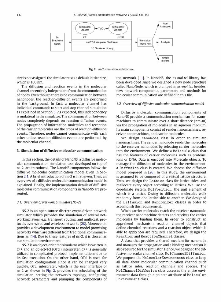
Fig. 2. ns-2 simulation architecture.
size is not assigned, the simulator uses a default lattice size,which is 100 nm.The diffusion and reaction events in the molecular
channel are entirely independent from the communicationof nodes. Even though there is no communication betweennanonodes, the reaction-diffusion events are performedin the background. In fact, a molecular channel hasindividual commands to start and stop channel simulationas explained in Section 3. As expected, this independencyis unilateral in the simulator. The communication betweennodes completely depends on reaction-diffusion events.The propagation of information molecules and receptionof the carrier molecules are the crops of reaction-diffusionevents. Therefore, nodes cannot communicate with eachother unless reaction-diffusion events are performed bythe molecular channel.
3. Simulation of diffusive molecular communication
In this section, the details of NanoNS, a diffusive molec-ular communication simulation tool developed on top ofns-2, are introduced. The NanoNS components follow thediffusive molecular communication model given in Sec-tion 2.1. A brief introduction of ns-2 is first given. Then, anoverview of a diffusivemolecular communicationmodel isexplained. Finally, the implementation details of diffusivemolecular communication components in NanoNS are pre-sented.
3.1. Overview of Network Simulator (NS-2)
NS-2 is an open source discrete event-driven networksimulator which provides the simulation of several net-working layers, e.g., transport, routing, and multicast, pro-tocols over wired and wireless networks [28]. Moreover, itprovides a development environment to model promisingnetworkswhich are different from traditional communica-tions as [14]. Due to these features of ns-2, it is chosen asour simulation environment.NS-2 is an object-oriented simulator which is written in
C++ and an object-Tcl (OTcl) interpreter. C++ is generallyutilized in complicated protocol implementations due toits fast execution. On the other hand, OTcl is used forsimulation configuration since it can be changed veryquickly. OTcl interpreter, which is the user interface ofns-2 as shown in Fig. 2, provides the scheduling of thesimulation, setting the network’s topology, configuringnetwork parameters and plumping the components of
the network [11]. In NanoNS, the ns-mol.tcl library hasbeen developed since we designed a new node structurecalled NanoNode, which is plumped in ns-mol.tcl, besides,new network components, parameters and methods formolecular communication are defined in this file.
3.2. Overview of diffusive molecular communication model
Diffusive molecular communication components ofNanoNS provide a communication mechanism for nano-machines to communicate over a short distance (nm-m)via the propagation of molecules in an aqueous medium.Its main components consist of sender nanomachines, re-ceiver nanomachines, and carrier molecules.We design NanoNode class in order to simulate
nanomachines. The sender nanonode sends the moleculesto the receiver nanonodes by releasing carrier moleculesinto the environment. We define a Molecule class thathas the features of carrier molecules such as proteins,ions or DNA. Data is encoded into Molecule objects. Tomanage the diffusion of molecules in the environment,a Diffusion class is created. We choose the diffusionmodel proposed in [26]. In this study, the environmentis assumed to be composed of a virtual lattice structure.Thus, we design the Lattice class for lattice sides, andreallocate every object according to lattices. We use thecoordinate system, MolPosition, the unit element ofwhich is a lattice. Owing to diffusion, molecules walkrandomly from one lattice side to another. We designedthe Diffusion and Randomizer classes in order toaccomplish this requirement.When carrier molecules reach the receiver nanonode,
the receiver nanomachine detects and receives the carriermolecules by binding them. In order to construct anapprehend mechanism, reaction channel objects thatdefine chemical reactions and a reaction object which isable to apply SSA are required. Therefore, we design theReaction and ReactionChannel classes.A class that provides a shared medium for nanonode
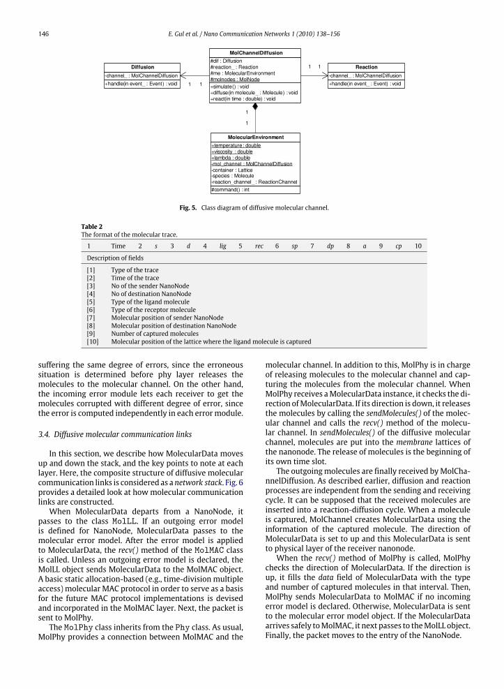
and manages the propagation and a binding mechanism isalso required for the simulator. Hence,we designed the dif-fusive molecular channel class, MolChannelDiffusion.We propose the MolecularEnvironment class to keepall data about molecular communication channel suchas lattice sides, reaction channels and species. TheMolChannelDiffusion class accesses the entire envi-ronment data through a pointer attribute of MolecularEnvironment class.
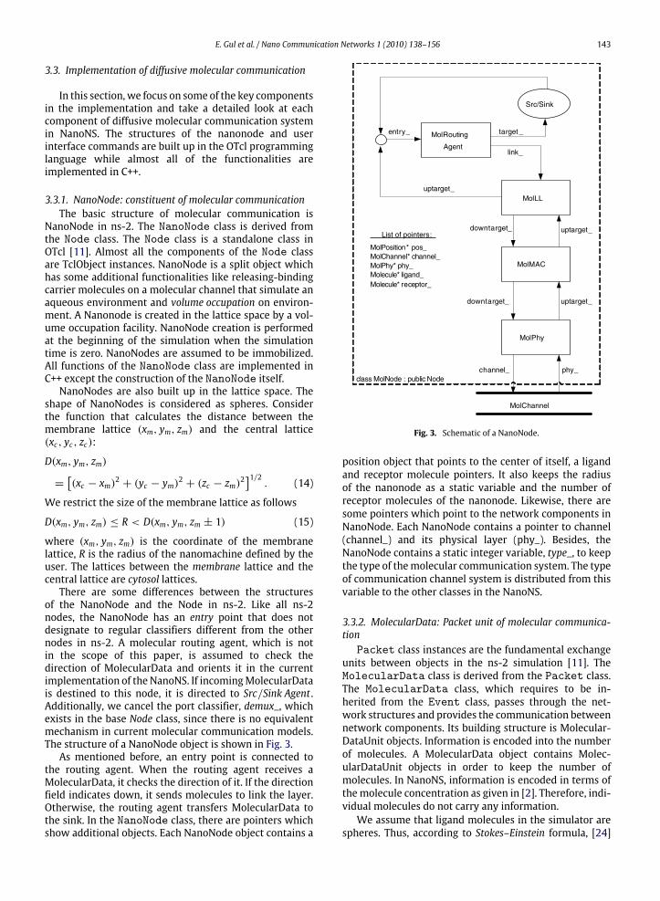
E. Gul et al. / Nano Communication Networks 1 (2010) 138–156 143
3.3. Implementation of diffusive molecular communication
In this section, we focus on some of the key componentsin the implementation and take a detailed look at eachcomponent of diffusive molecular communication systemin NanoNS. The structures of the nanonode and userinterface commands are built up in the OTcl programminglanguage while almost all of the functionalities areimplemented in C++.
3.3.1. NanoNode: constituent of molecular communicationThe basic structure of molecular communication is
NanoNode in ns-2. The NanoNode class is derived fromthe Node class. The Node class is a standalone class inOTcl [11]. Almost all the components of the Node classare TclObject instances. NanoNode is a split object whichhas some additional functionalities like releasing-bindingcarrier molecules on a molecular channel that simulate anaqueous environment and volume occupation on environ-ment. A Nanonode is created in the lattice space by a vol-ume occupation facility. NanoNode creation is performedat the beginning of the simulation when the simulationtime is zero. NanoNodes are assumed to be immobilized.All functions of the NanoNode class are implemented inC++ except the construction of the NanoNode itself.NanoNodes are also built up in the lattice space. The
shape of NanoNodes is considered as spheres. Considerthe function that calculates the distance between themembrane lattice (xm, ym, zm) and the central lattice(xc, yc, zc):
D(xm, ym, zm)
=[(xc − xm)2 + (yc − ym)2 + (zc − zm)2
]1/2. (14)
We restrict the size of the membrane lattice as follows
D(xm, ym, zm) ≤ R < D(xm, ym, zm ± 1) (15)
where (xm, ym, zm) is the coordinate of the membranelattice, R is the radius of the nanomachine defined by theuser. The lattices between the membrane lattice and thecentral lattice are cytosol lattices.There are some differences between the structures
of the NanoNode and the Node in ns-2. Like all ns-2nodes, the NanoNode has an entry point that does notdesignate to regular classifiers different from the othernodes in ns-2. A molecular routing agent, which is notin the scope of this paper, is assumed to check thedirection of MolecularData and orients it in the currentimplementation of the NanoNS. If incomingMolecularDatais destined to this node, it is directed to Src/Sink Agent .Additionally, we cancel the port classifier, demux_, whichexists in the base Node class, since there is no equivalentmechanism in current molecular communication models.The structure of a NanoNode object is shown in Fig. 3.As mentioned before, an entry point is connected to
the routing agent. When the routing agent receives aMolecularData, it checks the direction of it. If the directionfield indicates down, it sends molecules to link the layer.Otherwise, the routing agent transfers MolecularData tothe sink. In the NanoNode class, there are pointers whichshow additional objects. Each NanoNode object contains a
MolRouting
Agent
MolLL
MolMAC
MolPhy
Src/Sink
MolChannel
entry_
MolPosition* pos_ MolChannel* channel_MolPhy* phy_Molecule* ligand_Molecule* receptor_
List of pointers:
class MolNode : public Node
uptarget_
channel_
downtarget_
downtarget_
uptarget_
uptarget_
phy_
link_
target _
Fig. 3. Schematic of a NanoNode.
position object that points to the center of itself, a ligandand receptor molecule pointers. It also keeps the radiusof the nanonode as a static variable and the number ofreceptor molecules of the nanonode. Likewise, there aresome pointers which point to the network components inNanoNode. Each NanoNode contains a pointer to channel(channel_) and its physical layer (phy_). Besides, theNanoNode contains a static integer variable, type_, to keepthe type of themolecular communication system. The typeof communication channel system is distributed from thisvariable to the other classes in the NanoNS.
3.3.2. MolecularData: Packet unit of molecular communica-tion
Packet class instances are the fundamental exchangeunits between objects in the ns-2 simulation [11]. TheMolecularData class is derived from the Packet class.The MolecularData class, which requires to be in-herited from the Event class, passes through the net-work structures and provides the communication betweennetwork components. Its building structure is Molecular-DataUnit objects. Information is encoded into the numberof molecules. A MolecularData object contains Molec-ularDataUnit objects in order to keep the number ofmolecules. In NanoNS, information is encoded in terms ofthemolecule concentration as given in [2]. Therefore, indi-vidual molecules do not carry any information.We assume that ligand molecules in the simulator are
spheres. Thus, according to Stokes–Einstein formula, [24]
144 E. Gul et al. / Nano Communication Networks 1 (2010) 138–156
the diffusion coefficient of a ligand molecule is given asfollows
D =kT6πrη
(16)
where k is Boltzmann constant, T is the temperature of themedium, r is the radius of the sphere and η is the viscosityof the aqueous medium.
3.3.3. Diffusion: Propagation systemThe Diffusion class inherits from a TclObject class
since the type of diffusion object is determined by theuser via the diffusion parameter in the node configurationinterface. Currently, only one type of Diffusion model isimplemented; nevertheless, new diffusion models can beimplemented and joined into the simulator.TheDiffusion class is also derived from theHandler
class. When an event is ready, the handle method ofthe Handler derived class, Diffusion, is called. In thehandle function of the Diffusion class, a diffusion eventis triggered. The Diffusion class has an interface onlywith the MolChannelDiffusion class. The minimuminterface with other components brings modularity to thediffusion object.The basis of these diffusion processes is the multipar-
ticle LGA algorithm [26]. In this algorithm, the medium isdivided into lattices. Each lattice site holds a discrete num-ber of uniformly distributed particles. As a result of dif-fusion, molecules perform a random walk on the lattices.Molecules are distributed to neighbor lattices randomly.The exact position of a molecule is not necessary, only thelattice position of the molecule is needed. Every specieshas a particular diffusion coefficient. The diffusion time ofeach species is calculated with the lattice length and dif-fusion coefficient. If the number of molecules existing inthe lattice is less than the boundary value defined by theuser [26], the molecules move individually to a neighbor-ing lattice. If the number of molecules is larger than theboundary value, molecules are moved in bulk to a latticeaccording to Gaussian distribution.As mentioned before, membrane lattices act like a wall.
Molecules coming from outside the nanomachine cannotenter cytosol lattices. To simulate membrane lattices like awall, reflective boundary conditions are used. If moleculestry to diffuse into cytosol lattices, these molecules reflectfrom the cytosol lattices and stay in their local lattice.Every lattice has two different attributes in order to
hold the type and number of the molecules. One of themkeeps the current state, which keeps the actual moleculenumber in the lattice; while the other one keeps a tem-porary state, which keeps the molecule numbers in a dif-fusion state. During the diffusion process, the moleculesin the current state are distributed to temporary states ofneighboring lattice sides. At the end of the diffusion pro-cess, the temporary state is transferred to the current stateand reset.
3.3.4. Reaction: Capture mechanismThe Reaction class is derived from the TclObject
and Handler classes like a Diffusion object. Three types
of reaction models, i.e., NoReaction, Berg,Gillespie, can beselected via the Tcl script. In the NoReaction option, aligand molecule is captured whenever it collides with areceiver nanomachine. The Berg scheme implements thereactionmodel given in [7]. The Gillespie selection realizesSSA as described in Section 2.1.2. Some adaptations andassumptions added to SSA are as follows:
• We have a limited time interval to apply the algorithm,• If a reaction occurs in a vitro type lattice, the number ofreceptor and ligand molecules decreases,• If a reaction occurs in a membrane type lattice, thenumber of receptor molecules does not change; onlynumber of ligand molecule decreases,• There cannot be a chemical reaction inside a cytosollattice.
The identity element of the reaction mechanism is thereaction channel. The ReactionChannel class presentsthe chemical reaction that is defined by the user viathe set-reaction method of a molecular channel. In thesimulator, only the second order chemical reactions can bedefined. The types of molecules and diffusion coefficientrates define a reaction channel. The class diagram of areaction model is depicted in Fig. 4.
3.3.5. MolChannelDiffusion: Challenge of molecular commu-nicationThe challenging issue of a molecular communica-
tion simulator is the modeling of a molecular chan-nel. The MolChannelDiffusion class is derived fromthe Channel class. MolChannelDiffusion accessesto environmental data through a pointer that pointsto the MolecularEnvironment class. The MolecularEnvironment class keeps all the data about the molec-ular channel like a repository of simulator. The simulatorenvironment contains nanomachines, species, reactionchannels, and lattices.Lattice objects are the members of the Molecular
Environment class which keeps the entire latticemedium. There are three kinds of lattices for diffusivemolecular communication. These lattice types are cytosol,membrane, vitro. As mentioned before, nanonodes are con-structed withmembrane and cytosol lattices. The lattices inwhich the propagation of molecules occurs are expressedas vitro type lattices. Vitro type lattices behave like the out-sides of nanonodes. Molecules cannot diffuse into cytosollattices frommembrane and vitro lattices. The lattice side issupposed to keep the molecules in. The lattice class fulfillsthis requirement with twomaps, which keep themoleculetype and the number of molecules. One of them holds thecurrent state, the other keeps the temporary state of thelattice.In addition to keeping the lattices and lattice spaces, the
MolecularEnvironment class retains species and reac-tion channels in vectors. Other classes can reach and usethese data at any time of the simulation. It also keeps en-vironmental attributes, which affect the result of the sim-ulation, i.e., viscosity, temperature and lattice side length.In diffusive molecular communication, the molecular
channel keeps all nanonodes in the simulator. The diffusivemolecular channel is associatedwith diffusion and reaction
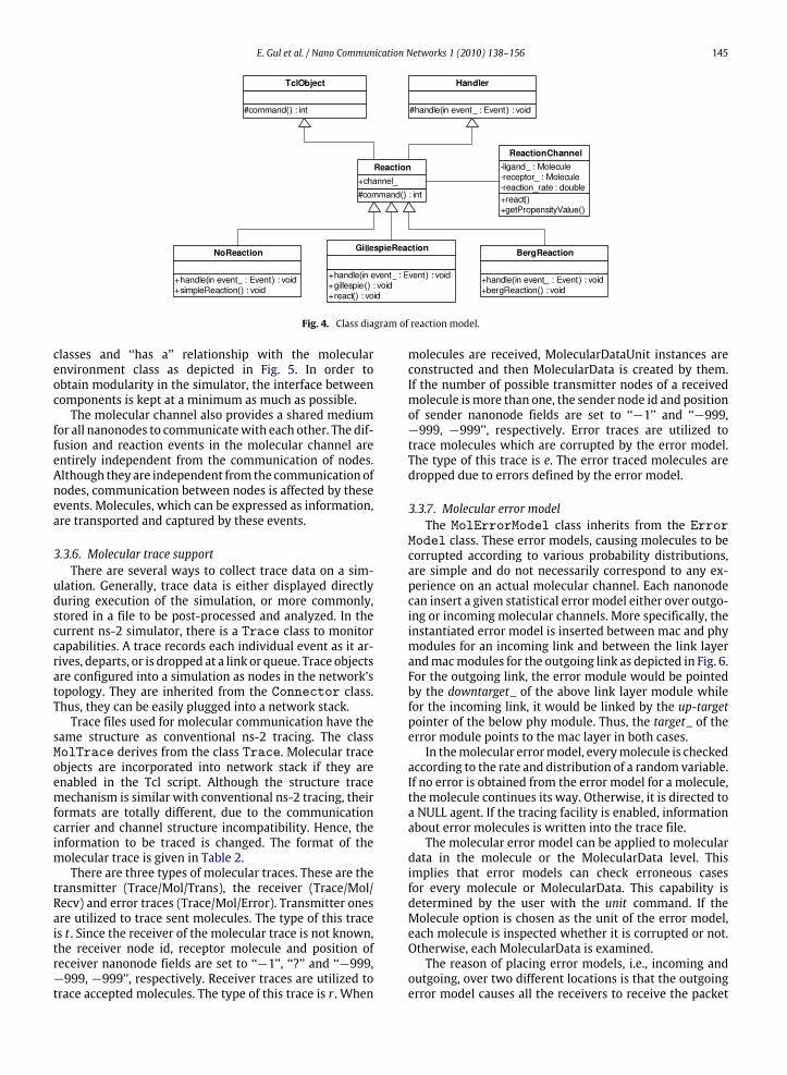
E. Gul et al. / Nano Communication Networks 1 (2010) 138–156 145
l l
l
ll
l
l
l l ll l
l
ll
lll
l
Fig. 4. Class diagram of reaction model.
classes and ‘‘has a’’ relationship with the molecularenvironment class as depicted in Fig. 5. In order toobtain modularity in the simulator, the interface betweencomponents is kept at a minimum as much as possible.The molecular channel also provides a shared medium
for all nanonodes to communicatewith each other. The dif-fusion and reaction events in the molecular channel areentirely independent from the communication of nodes.Although they are independent from the communication ofnodes, communication between nodes is affected by theseevents. Molecules, which can be expressed as information,are transported and captured by these events.
3.3.6. Molecular trace supportThere are several ways to collect trace data on a sim-
ulation. Generally, trace data is either displayed directlyduring execution of the simulation, or more commonly,stored in a file to be post-processed and analyzed. In thecurrent ns-2 simulator, there is a Trace class to monitorcapabilities. A trace records each individual event as it ar-rives, departs, or is dropped at a link or queue. Trace objectsare configured into a simulation as nodes in the network’stopology. They are inherited from the Connector class.Thus, they can be easily plugged into a network stack.Trace files used for molecular communication have the
same structure as conventional ns-2 tracing. The classMolTrace derives from the class Trace. Molecular traceobjects are incorporated into network stack if they areenabled in the Tcl script. Although the structure tracemechanism is similar with conventional ns-2 tracing, theirformats are totally different, due to the communicationcarrier and channel structure incompatibility. Hence, theinformation to be traced is changed. The format of themolecular trace is given in Table 2.There are three types of molecular traces. These are the
transmitter (Trace/Mol/Trans), the receiver (Trace/Mol/Recv) and error traces (Trace/Mol/Error). Transmitter onesare utilized to trace sent molecules. The type of this traceis t . Since the receiver of the molecular trace is not known,the receiver node id, receptor molecule and position ofreceiver nanonode fields are set to ‘‘−1’’, ‘‘?’’ and ‘‘−999,−999, −999’’, respectively. Receiver traces are utilized totrace accepted molecules. The type of this trace is r . When
molecules are received, MolecularDataUnit instances areconstructed and then MolecularData is created by them.If the number of possible transmitter nodes of a receivedmolecule ismore than one, the sender node id and positionof sender nanonode fields are set to ‘‘−1’’ and ‘‘−999,−999, −999’’, respectively. Error traces are utilized totrace molecules which are corrupted by the error model.The type of this trace is e. The error traced molecules aredropped due to errors defined by the error model.
3.3.7. Molecular error modelThe MolErrorModel class inherits from the Error
Model class. These error models, causing molecules to becorrupted according to various probability distributions,are simple and do not necessarily correspond to any ex-perience on an actual molecular channel. Each nanonodecan insert a given statistical error model either over outgo-ing or incoming molecular channels. More specifically, theinstantiated error model is inserted between mac and phymodules for an incoming link and between the link layerandmacmodules for the outgoing link as depicted in Fig. 6.For the outgoing link, the error module would be pointedby the downtarget_ of the above link layer module whilefor the incoming link, it would be linked by the up-targetpointer of the below phy module. Thus, the target_ of theerror module points to the mac layer in both cases.In themolecular errormodel, everymolecule is checked
according to the rate and distribution of a random variable.If no error is obtained from the error model for a molecule,the molecule continues its way. Otherwise, it is directed toa NULL agent. If the tracing facility is enabled, informationabout error molecules is written into the trace file.The molecular error model can be applied to molecular
data in the molecule or the MolecularData level. Thisimplies that error models can check erroneous casesfor every molecule or MolecularData. This capability isdetermined by the user with the unit command. If theMolecule option is chosen as the unit of the error model,each molecule is inspected whether it is corrupted or not.Otherwise, each MolecularData is examined.The reason of placing error models, i.e., incoming and
outgoing, over two different locations is that the outgoingerror model causes all the receivers to receive the packet
146 E. Gul et al. / Nano Communication Networks 1 (2010) 138–156
l l l
l
l l
ll l
l
ll
l
l
l
l l
ll
ll l l
l ll l
L
l l
Fig. 5. Class diagram of diffusive molecular channel.
Table 2The format of the molecular trace.
1 Time 2 s 3 d 4 lig 5 rec 6 sp 7 dp 8 a 9 cp 10
Description of fields
[1] Type of the trace[2] Time of the trace[3] No of the sender NanoNode[4] No of destination NanoNode[5] Type of the ligand molecule[6] Type of the receptor molecule[7] Molecular position of sender NanoNode[8] Molecular position of destination NanoNode[9] Number of captured molecules[10] Molecular position of the lattice where the ligand molecule is captured
suffering the same degree of errors, since the erroneoussituation is determined before phy layer releases themolecules to the molecular channel. On the other hand,the incoming error module lets each receiver to get themolecules corrupted with different degree of error, sincethe error is computed independently in each errormodule.
3.4. Diffusive molecular communication links
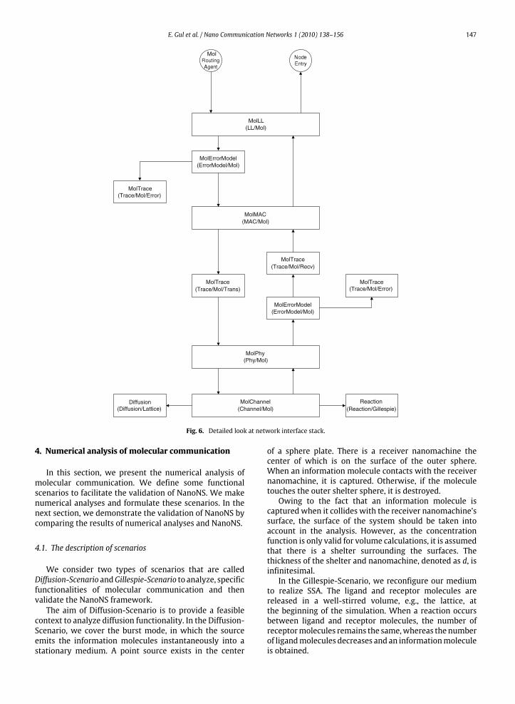
In this section, we describe how MolecularData movesup and down the stack, and the key points to note at eachlayer. Here, the composite structure of diffusive molecularcommunication links is considered as anetwork stack. Fig. 6provides a detailed look at howmolecular communicationlinks are constructed.When MolecularData departs from a NanoNode, it
passes to the class MolLL. If an outgoing error modelis defined for NanoNode, MolecularData passes to themolecular error model. After the error model is appliedto MolecularData, the recv() method of the MolMAC classis called. Unless an outgoing error model is declared, theMolLL object sends MolecularData to the MolMAC object.A basic static allocation-based (e.g., time-division multipleaccess) molecular MAC protocol in order to serve as a basisfor the future MAC protocol implementations is devisedand incorporated in the MolMAC layer. Next, the packet issent to MolPhy.The MolPhy class inherits from the Phy class. As usual,
MolPhy provides a connection between MolMAC and the
molecular channel. In addition to this, MolPhy is in chargeof releasing molecules to the molecular channel and cap-turing the molecules from the molecular channel. WhenMolPhy receives aMolecularData instance, it checks the di-rection ofMolecularData. If its direction is down, it releasesthe molecules by calling the sendMolecules() of the molec-ular channel and calls the recv() method of the molecu-lar channel. In sendMolecules() of the diffusive molecularchannel, molecules are put into the membrane lattices ofthe nanonode. The release of molecules is the beginning ofits own time slot.The outgoingmolecules are finally received byMolCha-
nnelDiffusion. As described earlier, diffusion and reactionprocesses are independent from the sending and receivingcycle. It can be supposed that the received molecules areinserted into a reaction-diffusion cycle. When a moleculeis captured, MolChannel creates MolecularData using theinformation of the captured molecule. The direction ofMolecularData is set to up and this MolecularData is sentto physical layer of the receiver nanonode.When the recv() method of MolPhy is called, MolPhy
checks the direction of MolecularData. If the direction isup, it fills the data field of MolecularData with the typeand number of captured molecules in that interval. Then,MolPhy sends MolecularData to MolMAC if no incomingerror model is declared. Otherwise, MolecularData is sentto the molecular error model object. If the MolecularDataarrives safely toMolMAC, it next passes to theMolLL object.Finally, the packet moves to the entry of the NanoNode.
E. Gul et al. / Nano Communication Networks 1 (2010) 138–156 147
Mol
MolLL(LL/Mol)
MolErrorModel(ErrorModel/Mol)
MolErrorModel(ErrorModel/Mol)
MolTrace
MolTrace
MolTraceMolTrace
(Trace/Mol/Error)
(Trace/Mol/Error)
(Trace/Mol/Recv)
(Trace/Mol/Trans)
MolMAC(MAC/Mol)
MolPhy(Phy/Mol)
MolChannel(Channel/Mol)
Diffusion(Diffusion/Lattice)
Reaction(Reaction/Gillespie)
Fig. 6. Detailed look at network interface stack.
4. Numerical analysis of molecular communication
In this section, we present the numerical analysis ofmolecular communication. We define some functionalscenarios to facilitate the validation of NanoNS. We makenumerical analyses and formulate these scenarios. In thenext section, we demonstrate the validation of NanoNS bycomparing the results of numerical analyses and NanoNS.
4.1. The description of scenarios
We consider two types of scenarios that are calledDiffusion-Scenario andGillespie-Scenario to analyze, specificfunctionalities of molecular communication and thenvalidate the NanoNS framework.The aim of Diffusion-Scenario is to provide a feasible
context to analyze diffusion functionality. In the Diffusion-Scenario, we cover the burst mode, in which the sourceemits the information molecules instantaneously into astationary medium. A point source exists in the center
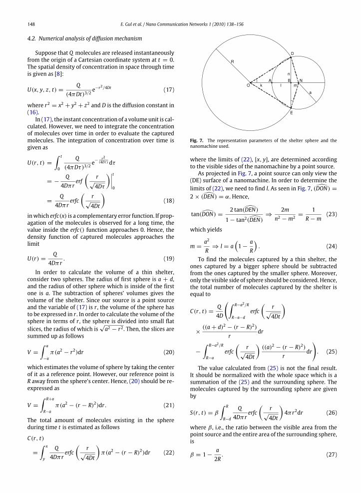
of a sphere plate. There is a receiver nanomachine thecenter of which is on the surface of the outer sphere.When an information molecule contacts with the receivernanomachine, it is captured. Otherwise, if the moleculetouches the outer shelter sphere, it is destroyed.Owing to the fact that an information molecule is
captured when it collides with the receiver nanomachine’ssurface, the surface of the system should be taken intoaccount in the analysis. However, as the concentrationfunction is only valid for volume calculations, it is assumedthat there is a shelter surrounding the surfaces. Thethickness of the shelter and nanomachine, denoted as d, isinfinitesimal.In the Gillespie-Scenario, we reconfigure our medium
to realize SSA. The ligand and receptor molecules arereleased in a well-stirred volume, e.g., the lattice, atthe beginning of the simulation. When a reaction occursbetween ligand and receptor molecules, the number ofreceptormolecules remains the same,whereas the numberof ligandmolecules decreases and an informationmoleculeis obtained.
148 E. Gul et al. / Nano Communication Networks 1 (2010) 138–156
4.2. Numerical analysis of diffusion mechanism
Suppose that Q molecules are released instantaneouslyfrom the origin of a Cartesian coordinate system at t = 0.The spatial density of concentration in space through timeis given as [8]:
U(x, y, z, t) =Q
(4πDt)3/2e−r
2/4Dt (17)
where r2 = x2 + y2 + z2 and D is the diffusion constant in(16).In (17), the instant concentration of a volume unit is cal-
culated. However, we need to integrate the concentrationof molecules over time in order to evaluate the capturedmolecules. The integration of concentration over time isgiven as
U(r, t) =∫ t
0
Q(4πDτ)3/2
e−r2(4Dτ) dτ
= −Q4Dπr
erf(
r√4Dτ
)∣∣∣∣t0
=Q4Dπr
erfc(
r√4Dt
)(18)
inwhich erfc(x) is a complementary error function. If prop-agation of the molecules is observed for a long time, thevalue inside the erfc() function approaches 0. Hence, thedensity function of captured molecules approaches thelimit
U(r) =Q4Dπr
. (19)
In order to calculate the volume of a thin shelter,consider two spheres. The radius of first sphere is a + d,and the radius of other sphere which is inside of the firstone is a. The subtraction of spheres’ volumes gives thevolume of the shelter. Since our source is a point sourceand the variable of (17) is r , the volume of the sphere hasto be expressed in r . In order to calculate the volume of thesphere in terms of r , the sphere is divided into small flatslices, the radius of which is
√a2 − r2. Then, the slices are
summed up as follows
V =∫ a
−aπ(a2 − r2)dr (20)
which estimates the volume of sphere by taking the centerof it as a reference point. However, our reference point isR away from the sphere’s center. Hence, (20) should be re-expressed as
V =∫ R+a
R−aπ(a2 − (r − R)2)dr. (21)
The total amount of molecules existing in the sphereduring time t is estimated as follows
C(r, t)
=
∫ x
y
Q4Dπr
erfc(
r√4Dt
)π(a2 − (r − R)2)dr (22)
Fig. 7. The representation parameters of the shelter sphere and thenanomachine used.
where the limits of (22), [x, y], are determined accordingto the visible sides of the nanomachine by a point source.As projected in Fig. 7, a point source can only view the
(DE) surface of a nanomachine. In order to determine thelimits of (22), we need to find l. As seen in Fig. 7, (D̂ON) =2× (D̂EN) = α. Hence,
tan(D̂ON) =2 tan(D̂EN)
1− tan2(D̂EN)⇒
2mn2 −m2
=1
R−m(23)
which yields
m =a2
R⇒ l = a
(1−
aR
). (24)
To find the molecules captured by a thin shelter, theones captured by a bigger sphere should be subtractedfrom the ones captured by the smaller sphere. Moreover,only the visible side of sphere should be considered. Hence,the total number of molecules captured by the shelter isequal to
C(r, t) =Q4D
(∫ R−a2/R
R−a−derfc
(r√4Dt
)×((a+ d)2 − (r − R)2)
rdr
−
∫ R−a2/R
R−aerfc
(r√4Dt
)((a)2 − (r − R)2)
rdr
). (25)
The value calculated from (25) is not the final result.It should be normalized with the whole space which is asummation of the (25) and the surrounding sphere. Themolecules captured by the surrounding sphere are givenby
S(r, t) = β∫ R
R−d
Q4Dπr
erfc(
r√4Dt
)4πr2dr (26)
where β , i.e., the ratio between the visible area from thepoint source and the entire area of the surrounding sphere,is
β = 1−a2R. (27)
E. Gul et al. / Nano Communication Networks 1 (2010) 138–156 149
After a long time period, the concentration ofmoleculesover time approaches a limit value. The limit values shouldbe used in the calculation of a normalization factor. As aresult, the normalization factor, NF , is given as
NF = limt→tsat
1C(r, t)+ S(r, t)
(28)
in which tsat is the saturation time in which the concentra-tion of molecules approaches the limit value.The multiplication of (25) and (28) provides the prob-
ability of crashing a molecule into the nanomachine withtime:
PCol(t) =C(r, t)
limt→tsat
(C(r, t)+ S(r, t)). (29)
The multiplication of PCol(t) with the total number of car-rier molecules, Q , gives the number of collided molecules,M(t), over time, i.e.,
M(t) = PCol(t)Q . (30)
To calculate the total number of collided molecules, weneed to consider that a long period of time passes, i.e.,t → ∞. Hence, the probability of collision of a moleculeafter a long period of time is
P∗Col =C(r,∞)
C(r,∞)+ S(r,∞). (31)
As in (19), when t → ∞, the erfc function approaches 1.Hence, the solution of P∗Col is as follows (32) is given in Box I.The total number of collided molecules is given as (33) inBox II. Although the diffusion coefficient, D, is one of theterms that effects the evaluation of the analytical diffusionmechanism as in (17), it has no impact on the total num-ber of collided molecules. The numerical results obtainedin this section are comparedwith experimental data in Sec-tion 5.1.
4.3. Numerical analysis of the Gillespie model
The goal of this section is to introduce a theoretical in-vestigation of SSA implementation of our reaction systemin the NanoNS. The chemical deterministic description ofthe system is given by the following ordinary differentialequation
∂CL(t)∂t= kCL(t)CR (34)
where CL(t) is the concentration of ligand molecules andCR is the concentration of receptor molecules. The concen-tration of ligandmolecules changeswith time,whereas thenumber of receptor molecules stays constant.In (34), the variables are in terms of concentration.
However, the input of the analysis is in terms of thenumber of ligand and receptor molecules. Therefore, weneed to map the concentration values into the number ofmolecules. The relation between the concentration and thenumber of molecules can be expressed as
C =nNV
(35)
where n is the number of molecules, N is the Avogadroconstant and V is the volume in units of liter . Hence, thesolution of (34) is given as
nL(t) = nL(0)e−knRtNV (36)
where nL(0) is the initial number of ligand molecules.We can figure out the characteristics of the captured
molecules number, nM(t), from nL(t). Since the ligandmolecules are transformed into captured molecules, wecan state that the number of captured molecules is thecomplement of the ligand molecules. The summationof ligand and captured molecules always equals theinitial number of ligand molecules. Hence, the number ofcaptured molecules can be expressed as follows
nM(t) = nL(0)(1− e−
knRtNV
). (37)
According to (37), the number of captured moleculesincreases with the reaction rate, the number of ligandsand receptors goes up, whereas it decreases as thevolume increases. (37) is used in the validation of SSA inSection 5.4.
5. Validation of the NanoNS framework
In this section, we present the validation of the NanoNSby comparing the outputs of the NanoNS and the results ofour analytical investigations. We also make a performanceevaluation of the NanoNS by using the utilization ratio,captured molecules over total molecules, of the NanoNSand analytical investigation results.
5.1. Validation of diffusion functionality
In this section, we validate and evaluate the perfor-mance of the diffusion functionality through capturedmolecules, the diffusion coefficient and the scalability ofNanoNS.
5.1.1. Validation by captured moleculesIn this section, we present a validation of the simulator
according to the number of captured molecules bythe NanoNS with time. We analyze the behavior ofcaptured molecules with respect to the ratio between thenanomachine’s radius and the shelter’s radius, a/R, and thenumber of released molecules.First, we analyze the behavior of captured molecules
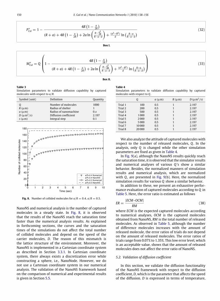
with respect to the ratio, a/R. We fix the simulationparameters except a and change a every 0.1 steps in theanalysis. The parameters used in the simulation are givenin Table 3. The simulator results and numerical analyses forratios 0.4 and 0.5 are shown in Fig. 8.As in Fig. 8, although numerical analyses and NanoNS
outputs exhibit a similar behavior for each a/R ratio,they do not exactly match. In fact, this mismatch resultsfrom the assumptions and constraints in the numericalanalysis. The significant point of the behavior of the
150 E. Gul et al. / Nano Communication Networks 1 (2010) 138–156
2)
P∗Col = 1−4R(1− a2R
)(R+ a)+ 4R
(1− a
2R
)+ 2a ln
(R− a
22R
R−a−d
)+
(a2−R2)d ln
( R−aR−a−d
) (3
Box I.
3)
M∗Col = Q1− 4R(1− a
2R
)(R+ a)+ 4R
(1− a
2R
)+ 2a ln
(R− a
22R
R−a−d
)+
(a2−R2)d ln
( R−aR−a−d
) (3
Box II.
Table 3Simulation parameters to validate diffusion capability by capturedmolecules with respect to a/R.
Symbol (unit) Definition Quantity
Q Number of molecules 1000R (µm) Radius of shelter 1a (µm) Radius of nanomachine 0.xD (µm2/s) Diffusion coefficient 2.197s (µm) Integral step 0.1
Fig. 8. Number of collided molecules for a/R = 0.4, a/R = 0.5.
NanoNS and numerical analysis is the number of capturedmolecules in a steady state. In Fig. 8, it is observedthat the results of the NanoNS reach the saturation timefaster than the numerical analysis results. As explainedin forthcoming sections, the curves and the saturationtimes of the simulations do not affect the total numberof collided molecules and depend on the speed of thecarrier molecules, D. The reason of this mismatch isthe lattice structure of the environment. Moreover, theNanoNS is implemented in a Cartesian coordinate systemas described in Section 3.3.1. In Cartesian coordinatesystem, there always exists a discretization error whileconstructing a sphere, i.e., NanoNode. However, we donot use a Cartesian coordinate system in our numericalanalysis. The validation of the NanoNS framework basedon the comparison of numerical and experimental resultsis given in Section 5.5.
Table 4Simulation parameters to validate diffusion capability by capturedmolecules with respect to Q .
Q a (µm) R (µm) D (µm2/s)
Trial 1 100 0.5 1 2.197Trial 2 200 0.5 1 2.197Trial 3 500 0.5 1 2.197Trial 4 1000 0.5 1 2.197Trial 5 2000 0.5 1 2.197Trial 6 5000 0.5 1 2.197Trial 7 10000 0.5 1 2.197Trial 8 20000 0.5 1 2.197
Wealso analyze the attitude of capturedmoleculeswithrespect to the number of released molecules, Q . In theanalysis, only Q is changed while the other simulationparameters are fixed as given in Table 4.In Fig. 9(a), although the NanoNS results quickly reach
the saturation time, it is observed that the simulator resultsand numerical analyses of various Q ’s show a similarbehavior. Besides, the normalized manners of simulationresults and numerical analysis, which are normalizedwith Q , are presented in Fig. 9(b). Here, the normalizedsimulation results for various Q show a similar behavior.In addition to these, we present an exhaustive perfor-
mance evaluation of captured molecules according to Q inTable 5. Here, the error ratio is estimated as follows
ER =|ECM–OCM|RM
(38)
where ECM is the expected captured molecules accordingto numerical analyses, OCM is the captured moleculesobtained from NanoNS, RM is the total number of releasedmolecules. As observed in Table 5, although the numberof difference molecules increases with the amount ofreleased molecule, the error ratios of trials do not dependon the amount of released molecules. The error ratios oftrials range from0.07% to 1.35%. This low error level, whichis an acceptable value, shows that the amount of releasedmolecules does not affect the error ratio of NanoNS.
5.2. Validation of diffusion coefficient
In this section, we validate the diffusion functionalityof the NanoNS framework with respect to the diffusioncoefficient,D, which is the parameter that affects the speedof the diffusion. D is expressed in terms of temperature,
E. Gul et al. / Nano Communication Networks 1 (2010) 138–156 151
a b
Fig. 9. (a) Behavior of collided molecules for Q = 2000, 5000, 10 000. (b) Normalized number of collided molecules for Q = 100, 1000, 20 000..
Table 5Error analysis of diffusion capability by captured molecules with respect to Q .
Obtained captured molecules Expected captured molecules Difference molecules Error ratio (%)
Trial 1 17.7 16.4 1.34 1.35Trial 2 32.9 32.7 0.14 0.07Trial 3 82.3 81.8 0.57 0.12Trial 4 171.5 163.5 7.95 0.8Trial 5 351.9 327.1 24.76 1.24Trial 6 874.9 817.7 57.13 1.14Trial 7 1742.8 1635.4 107.32 1.07Trial 8 3477.8 3270.9 206.94 1.03
Table 6Simulation parameters to analysis impacts of temperature, viscosity of the medium and the radius of the carrier molecules on simulation results.
Q a (µm) R (µm) T (K) η (J/K) rM (nm) D (µm2/s)
a
Trial 1 1000 0.3 1 150 0.001 100 1.098Trial 2 1000 0.3 1 300 0.001 100 2.197Trial 3 1000 0.3 1 600 0.001 100 4.394Trial 4 1000 0.3 1 900 0.001 100 6.591
b
Trial 5 1000 0.4 1 300 0.0005 100 4.394Trial 6 1000 0.4 1 300 0.001 100 2.197Trial 7 1000 0.4 1 300 0.002 100 1.098Trial 8 1000 0.4 1 300 0.003 100 0.732
c
Trial 9 1000 0.6 1 300 0.001 50 4.394Trial 10 1000 0.6 1 300 0.001 100 2.197Trial 11 1000 0.6 1 300 0.001 200 1.098Trial 12 1000 0.6 1 300 0.001 300 0.732
viscosity and the radius of the molecule as in (16). Firstof all, we analyze the effects of temperature, viscosity andthe radius of the molecule on simulation results. Then,we analyze the behavior of D on NanoNS. Moreover, wemeasure the performance of NanoNS with respect to thediffusion coefficient.If we consider our nanomachine as a unit volume, we
can use (18) in our analysis. In (18), the saturation time,tsat , can be expressed in terms of D as follows
tsat =C1
D(erfc ′(C2D))2(39)
in which erfc ′ is the inverse function of erfc , and C1, C2are constant values. From (39), it is observed that while Dincreases, tsat decreases and vice versa.We categorize the trials in order to inspect the effects
of temperature, viscosity and the radius of the molecule
on D individually. We analyze temperature, viscosity andthe radius ofmolecule in categories a, b and c , respectively.The simulation parameters and categorization of these aregiven in Table 6.In category a, we examine the impact of temperature
on simulation results. We fix all simulation parametersexcept temperature. In Fig. 10(a), while the temperatureincreases, which means an increase of D, the saturationtime of trials decreases as derived in (39). We examinethe influence of the viscosity of the medium on simulationresults in category b. We fix all simulation parametersexcept viscosity. In Fig. 10(b), while viscosity increases,which means a decrease of D, the saturation time oftrials increases. In category c , we inspect the effect ofthe radius of the carrier molecule on simulation results.We fix all simulation parameters except the radius of theinformation molecule. In Fig. 10(c), while the radius of
152 E. Gul et al. / Nano Communication Networks 1 (2010) 138–156
a b
c d
Fig. 10. (a) Impact of the temperature on simulation results. (b) Impact of the viscosity of the medium on simulation results. (c) Impact of the radius ofthe carrier molecule on simulation results. (d) Number of collided molecules for different diffusion coefficients.
Table 7Simulation parameters to validate the diffusion capability by the diffusioncoefficient.
Symbol (unit) Trial 1 Trial 2 Trial 3 Trial 4
Q 1000 1000 1000 1000R (µm) 1 1 1 1a (µm) 0.5 0.5 0.5 0.5s (µm) 0.1 0.1 0.1 0.1T (K) 300 100 100 100
η (J/K) 0.001 0.001 0.002 0.002rM (nm) 10 10 10 20D (µm2/s) 21.973 7.324 3.662 1.831
carrier molecule increases, whichmeans a decline ofD, thesaturation time of trials increases. In the rest of this section,we examine the impact of D on NanoNS. To achieve ourpurpose, the simulator is run with the parameters given inTable 7.Fig. 10(d) shows the number of collidedmolecules with
time behavior of all trials given in Table 7. The diffusioncoefficient has no impact on the total number of collidedmolecules according to (32). If we check the total numberof collided molecules of trials on Fig. 10(d), we see thatthey are in the range 170–180. The width of the range, 10,is an acceptable value in order to infer that the diffusioncoefficient does not affect the total number of collidedmolecules.In (39), if we neglect the impact of D on erfc ′, it turns
into a constant value. Based on this assumption, it is seenthat there is an inverse proportional relation between tsatand D as given in Fig. 11.
Fig. 11. The inverse proportional relation between tsat and D.
5.3. Validation of NanoNS scalability
We evaluate the performance of the simulator withrespect to the ratio of the radius of the nanomachine andthe radius of the shelter. We also examine the scalabilityof the NanoNS with respect to a/R in the validation andperformance evaluation. We make our scaling analysis fora random ratio, i.e., 0.4. We run the simulator with theparameters given in Table 8.Fig. 12(a) shows thenumber of capturedmoleculeswith
time for all trials given in Table 8. Since the lattice size of
E. Gul et al. / Nano Communication Networks 1 (2010) 138–156 153
a b
Fig. 12. (a) Number of collided molecules for different scales. (b) Utilization ratio for different scales.
Table 8Simulation parameters to validate the diffusion capability by simulatorscale.
Symbol (unit) Trial 1 Trial 2 Trial 3 Trial 4 Trial 5
Q 2000 2000 2000 2000 2000R (µm) 0.5 1 1.5 2.0 2.5a (µm) 0.2 0.4 0.6 0.8 1D (µm2/s) 2.197 2.197 2.197 2.197 2.197λ (nm) 100 100 100 100 100
the simulation is fixed, the distance between the sourceand the nanomachine is proportional to the number oflattices. If we consider our nanomachine as a unit volume,we can use (18) in our analysis. In (18), the saturation time,tsat , can be given in terms of r as follows
tsat =r2
C1(erfc ′(C2r))2(40)
in which erfc ′ is the inverse erfc function and C1, C2 areconstant values. It is seen that tsat is proportional to r2.Hence, the following relationship exists between the tsattrials
R1 < R2 < R3 < R4 < R5⇒ tSAT1 < tSAT2 < tSAT3 < tSAT4 < tSAT5. (41)
It is observed in Fig. 12(a) that the relationship amongtsat of simulator results is consistent with (41). If the ef-fect of scaling is analyzed considering (32), all parame-ters except (a
2−R2)d ln
( R−aR−a−d
)are proportional to the scal-
ing factor, whereas (a2−R2)d ln
( R−aR−a−d
)is proportional to k2.
Since (a2 − R2) is always negative, the number of col-lided molecules decreases when k increases as depicted
in Fig. 12(b). Here, it is observed that when the radius ofthe covering sphere is 0.5 µm, the utilization ratio is al-most the same for the NanoNS and the numerical analysis,whereas the ratio of the difference between them over theutilization ratio of the numerical analysis, error ratio, in-creases up to 20% as the radius goes up to 2.5µm.Althoughthe error ratio is approximately 20% for a large scaling fac-tor, the ratio of the difference over the total utilization ratiois approximately 2% which is an acceptable figure.
5.4. Validation of Gillespie model
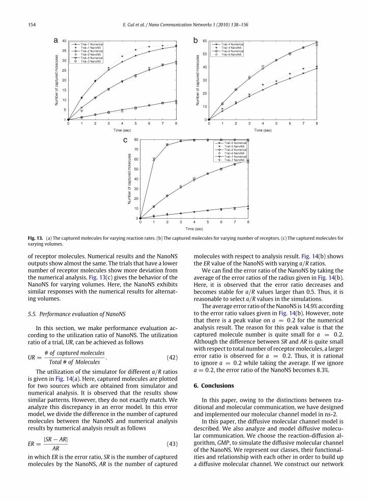
In this section, we validate and evaluate the perfor-mance of the SSA implementation of NanoNS. We makea numerical analysis of the SSA according to Gillespie-Scenario, in which ligand and receptor molecules are in alattice side, in Section 4.3. In the validation of the SSA im-plementation, we make our trials according to the param-eters given in Table 9.As derived in (37), the number of captured molecules
depends on initial number of ligand molecules, receptormolecules, reaction rate, volume of well-stirred mediumand time.We check the impact of each of these parametersin Fig. 13. In each figure, the response of the NanoNS andthe numerical analysis are plotted in order to validate eachof these parameters one by one.The impact of the reaction rate can be observed in
Fig. 13(a). Numerical result and the NanoNS output showalmost the same behavior. Trial 1, in which a deviation ex-ists between the NanoNS and numerical results, has thelargest reaction rate. Fig. 13(b) shows the behavior of theNanoNS and the numerical analysis for a varying number
Table 9Simulation parameters to validate SSA.
# of Ligand molecules # of receptor molecules Reaction rate (s/µm2) Volume side (nm)
Trial 1 40 20 0.01 100Trial 2 40 20 0.001 100Trial 3 40 20 0.005 100Trial 4 80 10 0.005 100Trial 5 80 20 0.005 200Trial 6 80 20 0.005 100Trial 7 80 20 0.005 50
154 E. Gul et al. / Nano Communication Networks 1 (2010) 138–156
a b
c
Fig. 13. (a) The captured molecules for varying reaction rates. (b) The captured molecules for varying number of receptors. (c) The captured molecules forvarying volumes.
of receptor molecules. Numerical results and the NanoNSoutputs show almost the same. The trials that have a lowernumber of receptor molecules show more deviation fromthe numerical analysis. Fig. 13(c) gives the behavior of theNanoNS for varying volumes. Here, the NanoNS exhibitssimilar responses with the numerical results for alternat-ing volumes.
5.5. Performance evaluation of NanoNS
In this section, we make performance evaluation ac-cording to the utilization ratio of NanoNS. The utilizationratio of a trial, UR, can be achieved as follows
UR =# of captured moleculesTotal # of Molecules
. (42)
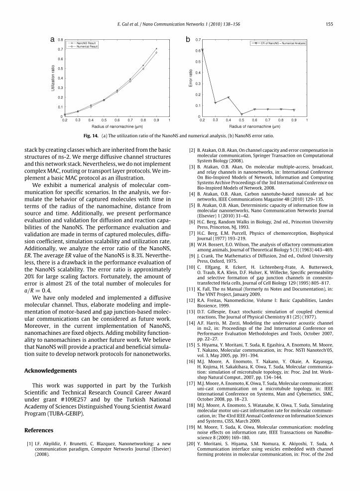
The utilization of the simulator for different a/R ratiosis given in Fig. 14(a). Here, captured molecules are plottedfor two sources which are obtained from simulator andnumerical analysis. It is observed that the results showsimilar patterns. However, they do not exactly match. Weanalyze this discrepancy in an error model. In this errormodel, we divide the difference in the number of capturedmolecules between the NanoNS and numerical analysisresults by numerical analysis result as follows
ER =|SR− AR|AR
(43)
in which ER is the error ratio, SR is the number of capturedmolecules by the NanoNS, AR is the number of captured
molecules with respect to analysis result. Fig. 14(b) showsthe ER value of the NanoNS with varying a/R ratios.We can find the error ratio of the NanoNS by taking the
average of the error ratios of the radius given in Fig. 14(b).Here, it is observed that the error ratio decreases andbecomes stable for a/R values larger than 0.5. Thus, it isreasonable to select a/R values in the simulations.The average error ratio of theNanoNS is 14.9% according
to the error ratio values given in Fig. 14(b). However, notethat there is a peak value on a = 0.2 for the numericalanalysis result. The reason for this peak value is that thecaptured molecule number is quite small for a = 0.2.Although the difference between SR and AR is quite smallwith respect to total number of receptormolecules, a largererror ratio is observed for a = 0.2. Thus, it is rationalto ignore a = 0.2 while taking the average. If we ignorea = 0.2, the error ratio of the NanoNS becomes 8.3%.
6. Conclusions
In this paper, owing to the distinctions between tra-ditional and molecular communication, we have designedand implemented our molecular channel model in ns-2.In this paper, the diffusive molecular channel model is
described. We also analyze and model diffusive molecu-lar communication. We choose the reaction-diffusion al-gorithm, GMP , to simulate the diffusive molecular channelof the NanoNS. We represent our classes, their functional-ities and relationship with each other in order to build upa diffusive molecular channel. We construct our network
E. Gul et al. / Nano Communication Networks 1 (2010) 138–156 155
a b
Fig. 14. (a) The utilization ratio of the NanoNS and numerical analysis. (b) NanoNS error ratio.
stack by creating classeswhich are inherited from the basicstructures of ns-2. We merge diffusive channel structuresand this network stack. Nevertheless,wedonot implementcomplexMAC, routing or transport layer protocols.We im-plement a basic MAC protocol as an illustration.We exhibit a numerical analysis of molecular com-
munication for specific scenarios. In the analysis, we for-mulate the behavior of captured molecules with time interms of the radius of the nanomachine, distance fromsource and time. Additionally, we present performanceevaluation and validation for diffusion and reaction capa-bilities of the NanoNS. The performance evaluation andvalidation are made in terms of captured molecules, diffu-sion coefficient, simulation scalability and utilization rate.Additionally, we analyze the error ratio of the NanoNS,ER. The average ER value of the NanoNS is 8.3%. Neverthe-less, there is a drawback in the performance evaluation ofthe NanoNS scalability. The error ratio is approximately20% for large scaling factors. Fortunately, the amount oferror is almost 2% of the total number of molecules fora/R = 0.4.We have only modeled and implemented a diffusive
molecular channel. Thus, elaborate modeling and imple-mentation of motor-based and gap junction-based molec-ular communications can be considered as future work.Moreover, in the current implementation of NanoNS,nanomachines are fixed objects. Addingmobility function-ality to nanomachines is another future work. We believethat NanoNSwill provide a practical and beneficial simula-tion suite to develop network protocols for nanonetworks.
Acknowledgements
This work was supported in part by the TurkishScientific and Technical Research Council Career Awardunder grant #109E257 and by the Turkish NationalAcademy of Sciences Distinguished Young Scientist AwardProgram (TUBA-GEBIP).
References
[1] I.F. Akyildiz, F. Brunetti, C. Blazquez, Nanonetworking: a newcommunication paradigm, Computer Networks Journal (Elsevier)(2008).
[2] B. Atakan, O.B. Akan, On channel capacity and error compensation inmolecular communication, Springer Transaction on ComputationalSystem Biology (2008).
[3] B. Atakan, O.B. Akan, On molecular multiple-access, broadcast,and relay channels in nanonetworks, in: International ConferenceOn Bio-Inspired Models of Network, Information and ComputingSystems Archive Proceedings of the 3rd International Conference onBio-Inspired Models of Network, 2008.
[4] B. Atakan, O.B. Akan, Carbon nanotube-based nanoscale ad hocnetworks, IEEE Communications Magazine 48 (2010) 129–135.
[5] B. Atakan, O.B. Akan, Deterministic capacity of information flow inmolecular nanonetworks, Nano Communication Networks Journal(Elsevier) 1 (2010) 31–42.
[6] H.C. Berg, Random Walks in Biology, 2nd ed., Princeton UniversityPress, Princeton, NJ, 1993.
[7] H.C. Berg, E.M. Purcell, Physics of chemoreception, BiophysicalJournal (1977) 193–219.
[8] W.H. Bossert, E.O. Wilson, The analysis of olfactory communicationamong animals, Journal of Theoretical Biology 5 (3) (1963) 443–469.
[9] J. Crank, The Mathematics of Diffusion, 2nd ed., Oxford UniversityPress, Oxford, 1975.
[10] C. Elfgang, R. Eckert, H. Lichtenberg-Frate, A. Butterweck,O. Traub, R.A. Klein, D.F. Hulser, K. Willecke, Specific permeabilityand selective formation of gap junction channels in connexin-transfected Hela cells, Journal of Cell Biology 129 (1995) 805–817.
[11] K. Fall, The ns Manual (formerly ns Notes and Documentation), in:The VINT Project, January 2009.
[12] R.A. Freitas, Nanomedicine, Volume I: Basic Capabilities, LandesBiosience, 1999.
[13] D.T. Gillespie, Exact stochastic simulation of coupled chemicalreactions, The Journal of Physical Chemistry 81 (25) (1977).
[14] A.F. Harris, M. Zorzi, Modeling the underwater acoustic channelin ns2, in: Proceedings of the 2nd International Conference onPerformance Evaluation Methodologies and Tools, October 2007,pp. 22–27.
[15] S. Hiyama, Y. Moritani, T. Suda, R. Egashira, A. Enomoto, M. Moore,T. Nakano, Molecular communication, in: Proc. NSTI Nanotech’05,vol. 3, May 2005, pp. 391–394.
[16] M.J. Moore, A. Enomoto, T. Nakano, Y. Okaie, A. Kayasuga,H. Kojima, H. Sakakibara, K. Oiwa, T. Suda, Molecular communica-tion: simulation of microtubule topology, in: Proc. 2nd Int. Work-shop Natural Comput., 2007, pp. 134–144.
[17] M.J. Moore, A. Enomoto, K. Oiwa, T. Suda,Molecular communication:uni-cast communication on a microtubule topology, in: IEEEInternational Conference on Systems, Man and Cybernetics, SMC,October 2008, pp. 18–23.
[18] M.J. Moore, A. Enomoto, S. Watanabe, K. Oiwa, T. Suda, Simulatingmolecular motor uni-cast information rate for molecular communi-cation, in: The 43rd IEEE Annual Conference on Information Sciencesand Systems, CISS, March 2009.
[19] M. Moore, T. Suda, K. Oiwa, Molecular communication: modelingnoise effects on information rate, IEEE Transactions on NanoBio-science 8 (2009) 169–180.
[20] Y. Moritani, S. Hiyama, S.M. Nomura, K. Akiyoshi, T. Suda, ACommunication interface using vesicles embedded with channelforming proteins in molecular communication, in: Proc. of the 2nd
156 E. Gul et al. / Nano Communication Networks 1 (2010) 138–156
ICST International Conference on Bio-Inspired Models of Network,Information and Computing Systems, BIONETICS, December 2007.
[21] Y. Moritani, S. Hiyama, T. Suda, Molecular communication amongnanomachines using vesicles, in: Proc. NSTI Nanotech’ 06, vol. 2,May2006, pp. 705–708.
[22] T. Nakano, T. Suda, T. Koujin, T. Haraguchi, Y. Hiraoka, Molecularcommunication through gap junction channels: system design,experiments and modeling, in: Proc. 2nd International Conferenceon Bio-Inspired Models of Network, Information, and ComputingSystems, BIONETICS 2007, December 2007.
[23] T. Nakano, T. Suda, M. Moore, R. Egashira, A. Enomoto, K. Arima,Molecular communication for nanomachines using intercellularcalcium signaling, in: Proc. 5th IEEE Conference on Nanotechnology,2005.
[24] G. Peskir, On the diffusion coefficient: the Einstein relationand beyond. Stochastic models, Stochastic Models 19 (3) (2003)383–405.
[25] M. Pierobon, I.F. Akyildiz, A physical channel model for molecularcommunication in nanonetworks, IEEE Journal on Selected Areas inCommunications (JSAC) 28 (2010) 602–611.
[26] J.V. Rodriguez, J.A. Kaandorp, M. Dobrzyński, J.G. Blom, Spatialstochastic modelling of the phosphoenolpyruvatedependent phos-photransferase (PTS) pathway in escherichia coli, Bioinformatics 22(15) (2006) 1895–1901.
[27] T. Suda, M. Moore, T. Nakano, R. Egashira, A. Enomoto, S.Hiyama, Y. Moritani, Exploratory research in molecular communi-cation between nanomachines, UCI Technical Report, 05–3, March2005.
[28] The network simulator [Online]. Available: http://www.isi.edu/nsnam/ns/ [accessed 29.07.10].
[29] P.J. Thomas, D.J. Spencer, S.K. Hampton, P. Park, J.P. Zurkus, Thediffusion mediated biochemical signal relay channel, in: Proc. 17thAnnual Conference on Neural Information Processing Systems,NIPS’03, 2003.
Ertan Gul received the B.S. and M.S. degrees inElectrical and Electronics Engineering from EgeUniversity, Izmir, Turkey and Middle East Tech-nical University (METU), Ankara, Turkey, in 2004and 2010, respectively. His current research in-terests are in nano-scale andmolecular commu-nications and nanonetworks.
Baris Atakan received the B.Sc. and M.Sc. de-grees in electrical and electronics engineeringfrom Ankara University and Middle East Tech-nical University, Ankara, Turkey, in 2000 and2005, respectively. He is currently a research as-sistant in theNext-generationWireless Commu-nication Laboratory and pursuing his Ph.D. de-gree at the Department of Electrical and Elec-tronics Engineering, Koc University. His currentresearch interests include nanoscale communi-cation, nanonetworks, and biologically-inspired
communication protocols for wireless networks.
Ozgur B. Akan received the B.S. and M.S. de-grees in Electrical and Electronics Engineeringfrom Bilkent University and Middle East Tech-nical University, Ankara, Turkey, in 1999 and2001, respectively. He received the Ph.D. de-gree in Electrical and Computer Engineeringfrom the Broadband and Wireless NetworkingLaboratory, School of Electrical and ComputerEngineering, Georgia Institute of Technology,Atlanta, in 2004. He is currently Associate Pro-fessor with the Department of Electrical and
Electronics Engineering, Koc University, Istanbul, Turkey. His current re-search interests are in wireless communications, bio-inspired communi-cations, nano-scale andmolecular communications, network informationtheory.Dr. Akan is an Associate Editor for IEEE Transactions on Vehicular
Technology, International Journal of Communication Systems (Wiley),Nano Communication Networks Journal (Elsevier). He served as an Editorfor ACM/SpringerWireless Networks (WINET) Journal (2004–2010), AreaEditor for AD HOC Networks Journal (Elsevier) (2004–2008), as a GuestEditor for several special issues, as the TPC Co-Chair for the 5th ICST/ACMInternational Conference on Nano-Networks (Nano-Net 2011), TPC Co-Chair for the 13th ACM International Conference on Modeling, Analysisand Simulation of Wireless and Mobile Systems (ACMMSWiM 2010), theGeneral Co-Chair for The Third International Conference on Bio-InspiredModels of Network, Information, and Computing Systems (ICST/IEEE BIO-NETICS 2008), the European Vice Chair for ICST/ACM Nano-Net 2007, anInternational Vice Chair for IEEE INFOCOM 2006, and in organizing com-mittees and technical program committees of many other internationalconferences. He is the Vice President for IEEE Communications Society—Turkey Section. He is an IEEE Senior Member (Communications Society),and a member of ACM. Dr. Akan received the IBM Faculty Award twice in2010 and 2008, Turkish Academy of Sciences Distinguished Young Scien-tist Award 2008 (TUBA-GEBIP).