1

Narrative Explanation of Econometric Demand Equations for Market Dominant Products Filed with Postal Regulatory Commission on January 22, 2014

Prepared for the Postal Regulatory Commission

2

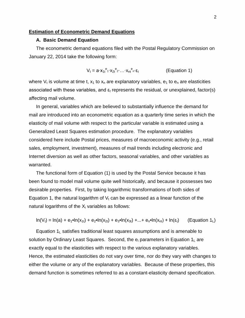
Estimation of Econometric Demand Equations A. Basic Demand Equation The econometric demand equations filed with the Postal Regulatory Commission on

January 22, 2014 take the following form:

Vt = a∙x1t

e1∙x2t

e2∙…∙xnt

en∙εt (Equation 1)

where Vt is volume at time t, x1 to xn are explanatory variables, e1 to en are elasticities

associated with these variables, and εt represents the residual, or unexplained, factor(s)

affecting mail volume.

In general, variables which are believed to substantially influence the demand for

mail are introduced into an econometric equation as a quarterly time series in which the

elasticity of mail volume with respect to the particular variable is estimated using a

Generalized Least Squares estimation procedure. The explanatory variables

considered here include Postal prices, measures of macroeconomic activity (e.g., retail

sales, employment, investment), measures of mail trends including electronic and

Internet diversion as well as other factors, seasonal variables, and other variables as

warranted.

The functional form of Equation (1) is used by the Postal Service because it has

been found to model mail volume quite well historically, and because it possesses two

desirable properties. First, by taking logarithmic transformations of both sides of

Equation 1, the natural logarithm of Vt can be expressed as a linear function of the

natural logarithms of the Xi variables as follows:

ln(Vt) = ln(a) + e1•ln(x1t) + e2•ln(x2t) + e3•ln(x3t) +...+ en•ln(xnt) + ln(εt) (Equation 1L) Equation 1L satisfies traditional least squares assumptions and is amenable to

solution by Ordinary Least Squares. Second, the ei parameters in Equation 1L are

exactly equal to the elasticities with respect to the various explanatory variables.

Hence, the estimated elasticities do not vary over time, nor do they vary with changes to

either the volume or any of the explanatory variables. Because of these properties, this

demand function is sometimes referred to as a constant-elasticity demand specification.

3

For explanatory variables which are logged in the equation, then, the coefficients

which come out of these demand equations can be interpreted directly as elasticities. B. Explanatory Variables 1. Price a. Own-Price Measures The starting point for traditional micro-economic theory is a demand equation that

relates quantity demanded to price. Quantity demanded is inversely related to price.

That is, if the price of a good were increased, the volume consumed of that good would

be expected to decline, all other things being equal.

This fundamental relationship of price to quantity is modeled in the Postal Service’s

demand equations by including the price of postage in each of the demand equations

estimated by the Postal Service for mail categories and services which have a price

(i.e., excluding Postal Penalty mail and Free for the Blind and Handicapped Mail).

The Postal prices entered into these demand equations are calculated as weighted

averages of the various rates within each particular category of mail. For example, the

price of First-Class single-piece letters is a weighted average of the single-piece letters

rate (46 cents), the additional ounce rate (20 cents), and the nonstandard surcharge (20

cents)1. Product-by-product billing determinants provide the components of the market

baskets which are used as weights in developing these price measures. The price

indices used in the demand equations filed with the Commission on January 22, 2014,

were constructed using FY 2012 billing determinants.

Looking at the historical relationship between mail volumes and Postal prices

suggests that mailers may not react immediately to changes in Postal rates. For some

types of mail it may take up to a year for the full effect of changes in Postal rates to

influence mail volumes. To account for the possibility of a lagged reaction to changes in

Postal prices on the demand for certain types of mail, the Postal price may be entered

into the demand equations lagged by up to four quarters. The exact number of lags

used is an empirical question which is answered on a case-by-case basis.

Prices are expressed in the Postal Service’s demand equations in real dollars. The

consumer price index (CPI-U) is used to deflate the prices.

1 Rates as of January 22, 2014.

4

In general, when the Postal Service refers to own-price elasticities, the reference is

to long-run own-price elasticities. The long-run own-price elasticity of a mail category is

equal to the sum of the coefficients on the current and lagged price of mail in the

relevant demand equation. The long-run own-price elasticity therefore reflects the

cumulative impact of price on mail volume after allowing time for all of the lag effects to

be felt.

b. Other Price Measures The price of postage is not the only price paid by most mailers to send a good or

service through the mail. For those cases where the non-Postal price of mail is

significant and for which a reliable time series of non-Postal prices is available, these

prices may also be included explicitly in the demand equations used to explain mail

volume, although there are no such examples in the demand equations presented here.

Prices of competing goods may also be included in some of the Postal Service’s

demand equations.

c. Postal Cross-Price Relationships Historically, several of the Postal Service’s econometric demand equations have

included cross-price measures with other Postal products, such as First-Class single-

piece and workshared letters and Bound Printed Matter and Media Mail. In some

cases, these cross-price variables entered the equations in the same way as the own-

price variables, i.e., as a measure of the average price of the product. In other cases,

however, cross-price variables were measured in relative terms (i.e., the difference

between the prices of two Postal products).

As has been the case for several years now, the econometric demand equations

filed with the Postal Regulatory Commission on January 22, 2014, do not include any

such cross-price variables. The exclusion of such variables was first discussed in some

detail in the response to the Chairman’s Information Request No. 8, question 5, which

was filed with the Commission on March 8, 2010. As explained in that response, the

decision of whether or not to include a particular cross-price relationship in a particular

econometric demand equation was made on a case-by-case basis. In all cases, the

5

overriding goal of all of the Postal Service’s econometric work is to produce the most

accurate volume forecasts possible. As a general rule, the most accurate volume

forecasts are obtained from econometric demand equations which best model the

historical demand for mail volume. So, while it ended up being the case that, in fact,

there were no cross-price or discount variables included in any of the econometric

demand equations filed on January 22, 2014, this was not the result of a general

decision to exclude all such variables from the Postal Service’s equation, but was,

instead, the result of a series of careful analyses of each of the Postal Service’s

individual demand equations.

This is not, however, to say that mailers may not at times shift from one mail

subclass to another in response to a change in Postal rates. In fact, however, such

changes tend to overwhelmingly be responses to specific and unusual changes in

relative rate structures associated with a specific rate change. Rather than attempting

to model such changes through a blunt one-size-fits-all instrument such as an

aggregate price index or an average discount level, the effect of such changes is,

instead, better modeled through the inclusion of either simple dummy variables or non-

linear Intervention analysis. Examples of such case-specific mailer shifts between mail

subclasses include the impact of R97-1 and R2006-1 on Standard Regular and ECR

mail volumes and the impact of MC96-1 on Standard Nonprofit and Nonprofit ECR mail

volumes.

6

2. Impact of the Economy on Mail Volumes In addition to being affected by prices, mail volumes are also affected by the state of

the economy. For example, as incomes rise, consumers are able to consume more,

and this is generally true of Postal Services which tend to rise during periods of strong

economic growth and stagnate or decline during recessions. A stronger economy is

also likely to increase business use of the mail. To model these relationships, the

demand equations used by the Postal Service typically include one or more

macroeconomic variables which relate mail volumes to general economic conditions.

a. Macroeconomic Variables Used Here Four key macroeconomic variables are used in the Postal Service’s econometric

market-dominant demand equations: employment, investment, mail-order retail sales,

and exports. These data are compiled by the United States government and are

obtained by the Postal Service from IHS Global Insight, a respected and independent

economic forecasting firm. At various times, consumption expenditures, personal

disposable income, gross domestic product (GDP), and the difference between actual

and potential GDP (the output gap) have also been explored as candidate explanatory

variables.

The specific variable choices are made on an equation-by-equation basis. The

decision process in choosing macroeconomic variables includes an effort to develop

equations which are both theoretically correct as well as empirically robust.

(1) Employment Total private employment is included in several of the Postal Service’s econometric

demand equations, including First-Class single-piece and workshared letters, cards,

and flats; Periodicals mail; Money Orders; and Post Office Boxes. Employment is an

excellent measure of the overall level of business activity in the economy. In many

cases, mail volume is not affected by the dollar value of economic transactions, so

much as by the number of such transactions. For example, the number of credit card

bills one receives does not necessarily go up as the total amount charged per card goes

up. While variables like GDP or retail sales may be good measures of the total dollar

amount of economic activity (e.g., the total amount charged per credit card),

7

employment appears to be a better measure of the number of business transactions

(e.g., number of credit card bills received).

Ultimately, the choice of which macroeconomic variable to use in a demand equation

is an empirical decision based on which variable best fits the volume data.

(2) Total Real Investment Advertising can be viewed as a type of business investment. As such, direct-mail

advertising volume is likely to be affected by the same factors which drive business

investment spending. To reflect this relationship, real gross private domestic

investment is included as an explanatory variable in the demand equations for Standard

Regular, Enhanced Carrier Route (ECR), Nonprofit, and Nonprofit ECR mail filed with

the Commission on January 22, 2014.

(3) Mail-Order Retail Sales First-Class Parcels, Bound Printed Matter, and Media Mail volumes consist, in large

part, of the delivery of products bought by the sender or recipient of the mail. This type

of mail volume derives almost directly from retail sales. More specifically, package

delivery services are largely a function of mail-order retail sales, that is, sales of goods

which are delivered to the consumer. Hence, mail-order retail sales (which include

sales identified as “electronic shopping”) are included directly in the demand equations

for First-Class Parcels, Bound Printed Matter, and Media and Library Rate Mail to reflect

this direct relationship between mail-order retail sales and these mail volumes.

(4) Exports As the primary indicator of outgoing international trade, the exports variable

characterizes the type of economic activity that generates outgoing international mail of

all classes. In particular, exports will generate business communications that are sent

by International First-Class Mail.

b. Long-Run versus Short-Run Macroeconomic Impacts In some cases, the demand for a product may be affected differently by short-run

fluctuations in the macro-economy (e.g., typical recessions) and longer-run macro-

economic factors (e.g. long-run trends). The demand equations filed with the

Commission on January 22, 2014, allow for differences between long-run and short-run

8

macroeconomic impacts on the demand for mail volume. This is done through the use

of filtered macroeconomic data where appropriate.

Most economic data present a combination of growth and fluctuations. The purpose

of a filter is to distinguish the effect of these two features of the economy on mail

volume. Distinctions of this nature are particularly important around economic turning

points. More broadly, distinctions between long-run and short-run macroeconomic

impacts have important implications for short-term and long-term forecasts.

For the demand equations filed by the Postal Service on January 22, 2014, the issue

of long-run versus short-run macroeconomic impacts was addressed by decomposing

the macroeconomic variable of interest, call it yt, into two components, so that one can

study their distinct relationships with mail volume. In general, this means re-writing the

time series yt as the sum of two series,

yt = Tt + Ct (Equation 2)

where Tt is the long-run, or Trend component of yt, and Ct is the short-run, or Cyclical

component of yt.

The method employed by the Postal Service to accomplish this decomposition is the

Hodrick-Prescott (H-P) filter proposed by Hodrick and Prescott (1997). The procedure is

a graduation method long used in actuarial science. For any time series, yt, the method

tries to estimate a smooth series st such that

1. The series, s, is close to y in the sense that the sum of squared errors are minimized.

2. The series, s, is smooth in the sense that its second derivatives (changes in

slopes) are sufficiently small.

Formally applying the H-P filter to a time series, yt, a series, st is estimated, such that

the following is minimized

21

1

21

1

2 ))()(()( −

−

=+

=

−−−+− ∑∑ t

T

tttt

T

ttt sssssy λ

(Equation 3)

where yt is the time series (with T observations) to be decomposed, st is the smooth

series or trend component, and λ is the weight (or penalty) on the sum of changes in

slopes of st.

9

3. The Internet and Electronic Diversion One of the most significant issues facing the Postal Service in recent decades

has been the threat, both realized and potential, of electronic diversion of mail. E-mail

has emerged as a potent substitute for personal letters and business correspondence.

Bills can be paid online, and more and more consumers are also receiving bills and

statements through the Internet rather than through the mail. Virtually all magazines

and newspapers now have an online edition as a complement to their print editions, and

in some cases, the print edition has been eliminated in favor of an all-online format.

Understanding the emergence of the Internet and its role vis-à-vis the mail is critical in

understanding mail volume, both today and in the future.

There are two general dimensions to the Internet which are important to understand

in assessing the extent to which the Internet, and other electronic alternatives, may

serve as possible substitutes for mail volume: the breadth of Internet usage and the

depth of Internet usage.

i. Breadth of Internet Use The breadth of Internet usage refers generally to the number of people online. As

more people use the Internet, there are simply more people for whom the Internet is

available as a substitute for the mail.

Increases in the breadth of Internet use can explain a large share of historical

electronic diversion. Moving forward, however, further increases in the breadth of

Internet use are likely to be considerably less significant in explaining future diversion.

ii. Depth of Internet Use The depth of Internet usage refers to the number of things which an individual does

on the Internet. As the depth of Internet usage increases for a particular person, the

number of activities for which the Internet can substitute for mail may increase, thereby

increasing the overall level of substitution of the Internet for mail volume, even in the

absence of an increase in the number of Internet users.

The breadth and depth of Internet usage have both been important in understanding

the impact of the Internet on mail volumes historically. However, moving forward, the

depth of Internet usage is a much more important consideration. The reason for this is

10

that the breadth of Internet usage has a natural ceiling. Eventually, everybody who

would ever obtain Internet access will actually have Internet access. At that point, the

only source of increasing electronic diversion of the mail will be an increasing depth of

Internet usage. Hence, in measuring the impact of the Internet and other electronic

alternatives on mail volumes, it is important to measure the impact not only of the

breadth of Internet usage in the United States, but the depth of Internet (and other

electronic) usage as well.

Beginning in the early 2000s, the Postal Service has included one or more explicit

measures of Internet usage in several of its demand equations as a means of capturing

the impact of the Internet (and other electronic delivery alternatives) on mail volumes.

These variables – which included consumption expenditures on Internet Service

Providers, the number of households with Broadband Internet access, and the number

of Global Internet Servers - reflect primarily the breadth of Internet use – i.e., the

number of people on the Internet. As noted above, however, the story of Internet

diversion of mail has more recently been a story of increasing depth of Internet use.

To better measure the increasing depth of Internet use, the Postal Service’s

methodology for modeling Internet and other electronic diversion has changed more

recently. For the market-dominant demand equations filed with the Commission on

January 22, 2014, diversion is not modeled via explicit Internet variables, but, instead, is

measured through a series of simple linear time trends which start at various times

within the sample periods over which the Postal Service’s demand equations are

estimated.

Diversion trends of this kind are estimated in several of the Postal Service’s demand

equations, including all of First-Class Mail, Periodicals Mail, Media Mail, and Money

Orders. Time trends of this type are special cases of Intervention Analysis. The

technical details of Intervention Analysis are described later in this document.

11

4. The Great Recession Even after one controls for differences in the impact of long-run and short-run

macroeconomic impacts on mail volumes, the most recent recession appears to have

had a larger than expected negative impact on many categories of mail volume. Some

earlier work at the Postal Service dealt with these unique impacts of the ‘Great

Recession’ by looking at filtered macro-economic data, focusing on time periods where

the “trend” component of these variables turned negative.

More recently, the Postal Service has attempted to model the unique impacts of the

Great Recession on mail volumes using Intervention Analysis techniques. The

technical details of Intervention Analysis are described next.

5. Intervention Analysis

In some cases, mail volumes may be affected by unique events, or “interventions”.

Oftentimes, the effect of such factors can be modeled via simple trend or dummy

variables. In other cases, however, the impact of such “interventions” on mail volumes

may be more complicated than can be fully captured by a simple variable or variables.

In such cases, a more elaborate non-linear Intervention analysis is undertaken to more

accurately model the impact of some factors on some types of mail.

Two examples of Interventions for which this type of analysis is undertaken are the

two factors just discussed: Internet Diversion and the Great Recession.

a. Non-Linear Intervention Intervention analysis is a time series technique which allows one to identify the

effects of an event over time. An “intervention” is an event which affects the demand for

a given product. There are essentially three different types of impact of intervention

events: step functions, pulse functions, and trends. A generalized Intervention Analysis

technique allows for a functional form which is flexible enough to accommodate all of

these possibilities as dictated by the underlying data. This function is called the transfer

function.

The role of the transfer function is to allow the input variable to affect the volume in

different ways and rates over time. Therefore, the impact of an intervention on volume is

12

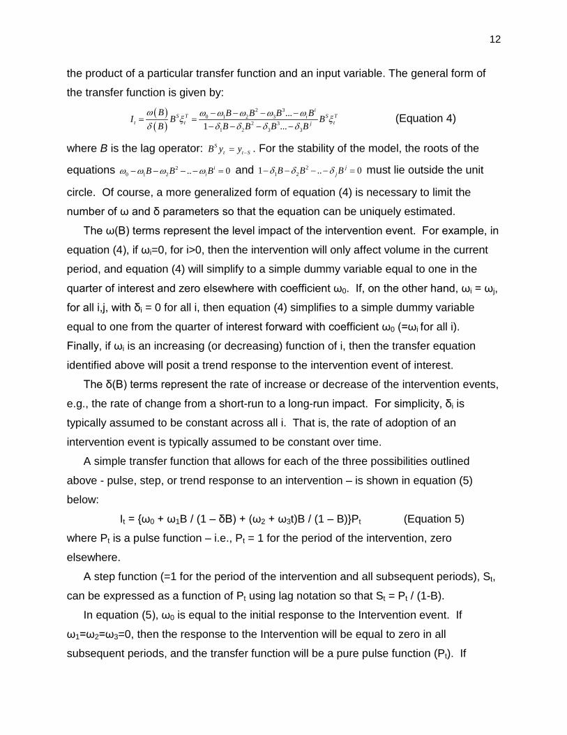
the product of a particular transfer function and an input variable. The general form of

the transfer function is given by:

( )( )

2 30 1 2 3

2 31 2 3 3

...1 ...

iS T S Ti

t t tj

B B B B BI B BB B B B B

ω ω ω ω ω ωξ ξδ δ δ δ δ

− − − −= =

− − − − (Equation 4)

where B is the lag operator: St t SB y y −= . For the stability of the model, the roots of the

equations 20 1 2 .. 0i

iB B Bω ω ω ω− − − − = and 21 21 .. 0j

jB B Bδ δ δ− − − − = must lie outside the unit

circle. Of course, a more generalized form of equation (4) is necessary to limit the

number of ω and δ parameters so that the equation can be uniquely estimated.

The ω(B) terms represent the level impact of the intervention event. For example, in

equation (4), if ωi=0, for i>0, then the intervention will only affect volume in the current

period, and equation (4) will simplify to a simple dummy variable equal to one in the

quarter of interest and zero elsewhere with coefficient ω0. If, on the other hand, ωi = ωj,

for all i,j, with δi = 0 for all i, then equation (4) simplifies to a simple dummy variable

equal to one from the quarter of interest forward with coefficient ω0 (=ωi for all i).

Finally, if ωi is an increasing (or decreasing) function of i, then the transfer equation

identified above will posit a trend response to the intervention event of interest.

The δ(B) terms represent the rate of increase or decrease of the intervention events,

e.g., the rate of change from a short-run to a long-run impact. For simplicity, δi is

typically assumed to be constant across all i. That is, the rate of adoption of an

intervention event is typically assumed to be constant over time.

A simple transfer function that allows for each of the three possibilities outlined

above - pulse, step, or trend response to an intervention – is shown in equation (5)

below:

It = {ω0 + ω1B / (1 – δB) + (ω2 + ω3t)B / (1 – B)}Pt (Equation 5)

where Pt is a pulse function – i.e., Pt = 1 for the period of the intervention, zero

elsewhere.

A step function (=1 for the period of the intervention and all subsequent periods), St,

can be expressed as a function of Pt using lag notation so that St = Pt / (1-B).

In equation (5), ω0 is equal to the initial response to the Intervention event. If

ω1=ω2=ω3=0, then the response to the Intervention will be equal to zero in all

subsequent periods, and the transfer function will be a pure pulse function (Pt). If

13

ω0=ω1 and δ=ω2=ω3=0, then the transfer function will be a pure step function (St = Pt /

(1-B)). If ω1=ω2=0 and ω0= ω3, then the transfer function will be a pure linear trend. If,

on the other hand, none of these equalities are realized, then equation (5) will explain a

more flexible transfer function as dictated by the observed data.

The functional form of equation (5), which expresses the transfer function as a

function of the lag operators may not be intuitively obvious. Re-expressing the lag

operator notation here into more conventional notation yields equation (6):

It = ω0·Pt + ω1·(Pt-1+δ1Pt-2+δ2Pt-3+…) + ω2·St + ω3·Tt·St (Equation 6)

where, as noted above, Pt is equal to one during the period of the intervention, zero

elsewhere (both before and after), St is equal to zero prior to the intervention event

being modeled, and equal to one thereafter, and T is a time trend equal to zero at the

point of the intervention event, increasing by one each quarter thereafter.

While equation (6) is a function of only 5 parameters – δ and ωi for i = 0 to 3 – it

nonetheless technically requires the inclusion of an infinite number of terms in the

demand equation of interest. It turns out, however, that, at any given point in time, all of

the Pt-i terms is equal to zero except for, at most, one. To see this, one can re-write

equation (6) as follows:

It = ω0·Pt + ω1·Σi=1∞(δi-1Pt-i) + ω2·St + ω3·Tt·St

When Tt = 1, the value of Pt-1 = 1, Pt-i = 0, for all i≠1. Similarly, when Tt = 2, the

value of Pt-2 = 1, Pt-i = 0, for all i≠2. So, instead of a sum over all values of Pt-i one can

instead replace i with Tt-1 in the above equation. That is,

It = ω0·Pt + ω1·St·(δTt-1) + ω2·St + ω3·Tt·St (Equation 7)

Intervention variables of the form in equation (7) are then added to the Postal

Service’s econometric demand equations as necessary. The Intervention parameters -

ω0, ω1, ω2, ω3, and δ – are estimated simultaneous with the other econometric

parameters using non-linear least squares.

As noted above, Intervention Analysis of this type is used to model unique aspects

of the ‘Great Recession’ on several classes of mail: most significantly, Standard Mail.

Other “interventions” which are modeled in this way include the impact of R97-1 rates

(which priced Standard Regular automation 5-digit letters below ECR basic letters) on

Standard Regular and ECR mail volumes. In this case, the initial impact was modestly

14

strong, but the negative impact grew over time, as mailers gradually adapted their

mailing procedures to take advantage of the lower Regular Automation rates.

b. Time Trends It is always desirable to be able to explain the behavior of a variable that is being

estimated econometrically as a function of other observable variables. Often, however,

the behavior of a variable is due to factors that do not easily lend themselves to capture

within a time series variable suitable for inclusion in an econometric experiment. It is

not uncommon for such phenomena to be modeled in part through the use of trend

variables. For example, it has been found by the Postal Service (and others2) that trend

variables do a better job of modeling the impact of electronic diversion on mail volume

than specific measures of Internet usage, which do not necessarily reflect the gradual

substitution of the Internet for correspondence and transactions which had previously

been undertaken via the mail.

Given that trend variables are needed within particular demand equations, an

equally important question becomes what forms these trend variables ought to take.

A trend is a trend is a trend But the question is, will it end? Will it alter its course Through some unforeseen force, And come to a premature end? Sir Alec Cairncross

It is not sufficient to merely plug linear time trends into all of one’s econometric

equations and project these trends to continue unabated throughout the forecast period.

Rather, it is important to evaluate every demand equation individually and determine the

appropriate trend specification for each equation, if any.

Many of the demand equations filed with the Commission on January 22, 2014,

including the Periodicals Mail equation, three of the four Standard Mail equation, and

most of the Special Service equations, included full-sample linear time trends to account

2 e.g., Veruete-McKay, Leticia; Soteri, Soterios; Nankervis, John C.; and Rodriguez, Frank (2011) "Letter Traffic Demand in the UK: An Analysis by Product and Envelope Content Type," Review of Network Economics: Vol. 10: Issue 3, Article 10.

15

for long-run trends in the volumes of these types of mail, for which economic sources do

not readily lend themselves to inclusion in an econometric time series equation. Such

long-run changes in mail volume are therefore most readily modeled by a simple trend

variable.

Some of the Postal Service’s demand equations include alternate trend

specifications. The Delivery and Signature Confirmation equations, for example,

include some logistic trend terms which more accurately reflect the rapid initial growth,

the rate of which declines over time, which often characterizes the early history of new

products. A similar logistic trend is also included in the First-Class workshared letters,

cards, and flats equation to model the increasing usage of worksharing discounts by

mailers in previous years, the rate of increase of which has slowed significantly more

recently.

Finally, several equations include linear time trends over only a portion of their

sample period. These trends capture new and changing influences which have affected

mail volumes, including the introduction and expansion of Internet and other types of

electronic diversion as well as changes in long-run mail trends that were caused by the

Great Recession. Trends of this nature are included, for example, in the demand

equations for First-Class Single-Piece and Workshared letters, cards, and flats;

Periodicals Mail; Media and Library Rate Mail; as well as Money Orders.

Time trends of this type are special cases of the non-linear intervention analysis

outlined above.

c. Dummy Variables In some cases, the effect of specific events may be modeled using simple dummy

variables. For example, certain equations include dummy variables for some rate or

classification changes that are inadequately modeled by the price indices used here.

Dummy variables of this type are special cases of the non-linear intervention analysis

outlined above.

6. Seasonality Postal Calendar

The volume data used in modeling the demand for mail are quarterly. Before 2004,

the Postal Service reported data using a 52-week Postal calendar composed of thirteen

16

28-day accounting periods.3 Because the 52-week Postal year was only 364 days long,

the beginning of the Postal year, as well as the beginning of each Postal quarter, shifted

over time relative to the traditional Gregorian calendar. Specifically, the Postal calendar

lost five days every four years relative to the Gregorian calendar. This created some

unique difficulties in modeling the seasonality of mail volumes.

For example, prior to 1983, Christmas Day fell in the first quarter of the Postal year

(which began in the previous Fall). After 1983, however, Christmas Day fell within the

second Postal quarter. Between Postal Fiscal Year 1983 (PFY 1983) and PFY 1999

(the last year for which Postal quarterly data are used here), the second Postal quarter

gained the 20 days immediately preceding Christmas (December 5 through December

24) which are among the Postal Service’s heaviest days in terms of mail volume. Not

surprisingly, therefore, the relative volumes of mail in Postal Quarter 1 and Postal

Quarter 2 changed over this time period for most mail categories, as Christmas-related

mailings shifted from the first Postal quarter to the second Postal quarter, solely

because of the effect of the Postal Service’s moving calendar.

This shift created a difficulty in modeling the seasonal pattern of mail volume using

traditional econometric techniques, such as simple quarterly dummy variables. If the

seasonal pattern of mail volume was due to seasonal variations within the Gregorian

calendar (e.g., Christmas), then the perceived seasonal pattern across Postal quarters

may not have been constant over time, even if the true seasonal pattern across periods

of the Gregorian calendar was constant over time.

Seasonal Variables, pre-2000

For demand equations whose sample period begins before 2000Q1, the seasonal

variables included in the Postal Service’s econometric demand equations are tied to the

Gregorian calendar. This means that they vary over the Postal calendar prior to 2000.

For demand equations whose sample period begins in 2000Q1 or later, Postal quarters

line up perfectly with the Gregorian calendar over the full sample period. In these

cases, the Postal Service’s econometric demand equations include simple quarterly 3 Postal Service volume data for Fiscal Years 2000 through 2003 were re-stated by Gregorian quarter at the time of this change in the Postal Service’s calendar. These re-stated data are used here to estimate the Postal Service’s demand equations.

17

dummy variables to model seasonality. Even in these latter cases, however, the impact

of Saturdays and Sundays is modeled empirically (in fact, it is only the time period since

2000Q1 where the number of Saturdays and Sundays within a particular quarter vary

over time).

In the past, the seasonal variables used to model seasonality prior to 2000Q1 were

discrete seasonal variables which measured the share of the relevant Postal quarter

which fell within a particular Gregorian time period. Recently, these have been changed

to a series of variables which allow for smoother seasonal transitions over time.

There are 12 seasonal variables, tied to 12 “target dates”: specifically, the 15th of

each month. Daily values associated with each of these variables are calculated such

that any given date has non-zero values for the 2 “target dates” closest to it such that

the sum of the two values associated with a particular date is equal to one and the

weight on a particular date decreases as one gets farther away from it and increases as

it gets closer to the target date.

Consider the example of the time period between November 15th and December

15th. The two “target dates” associated with these dates are November 15th (Nov15)

and December 15th (Dec15).

For November 15th, the value of Nov15 is set equal to 1; the value of Dec15 is set equal to zero. There are 30 days between November 15 and December 15. Hence, the values associated with Nov15 and Dec15 change by (1/30) per day over this time period. For November 16th, the value of Nov15 is set equal to 29/30 (1 – 1/30), and the value of Dec15 is set equal to 1/30 (0 + 1/30). For November 17th, the value of Nov15 is set equal to 28/30 (29/30 – 1/30), and the value of Dec15 is set equal to 2/30. … For December 14th, the value of Nov15 is set equal to 1/30, and the value of Dec15 is set equal to 29/30. For December 15th, the value of Nov15 is set equal to zero and the value of Dec15 is set equal to one.

The value of, say, Nov15, for a particular quarter is then simply equal to the average

daily value of Nov15 for the dates with the quarter of interest. For these calculations, all

days are treated equally (i.e., no adjustments are made for Saturdays, Sundays, or

18

Postal holidays). Because of this, the values of these variables are constant within a

particular Postal quarter since 20004. For example, the value of Nov15 is equal to

0.3315 in every Postal Quarter 1, while the value of Dec15 is equal to 0.2947 in every

Postal Quarter 1 (and 0.0372 in every Postal Quarter 2, since the time period from Jan.

1 – Jan. 14 is between the target dates of December 15 and January 15).

In addition to these twelve seasonal variables, a thirteenth variable is created called

CHRISTMAS. This variable is keyed to a single date as above: December 22nd, but

only operates in the three weeks before this date, with the variable having a value (1/21)

less than the next day (i.e., December 22 = 1, December 21 = (20/21), December 20 =

(19/21), …, December 2 = (1/21), all other dates = 0). As with the monthly variables

above, all days are treated equally in calculating CHRISTMAS, so that it has a constant

value in Postal Quarter 1 since 2000 (11/92 = 0.1196).

Adjoining seasons for which the coefficients are similar in sign and magnitude are

combined in some cases.5 These constraints across seasons are made on an

equation-by-equation basis. The criterion used for this constraining process is generally

to minimize the mean-squared error of the equation (which is equal to the sum of

squared residuals divided by degrees of freedom).

Changes to Seasonal Pattern over Time

In some cases, the seasonal pattern of certain mail categories appears to have

changed somewhat over time. In these cases, additional or alternate seasonal

variables may be introduced into the equation over sub-samples of the relevant sample

period. In most cases, these take the form of simple quarterly dummies which start at

some time after 2000. For example, the First-Class single-piece letters, cards, and flats

equation includes a dummy variable equal to one in the first Postal quarter starting in

2008Q1; the Standard Regular Mail demand equation includes dummy variables equal

to one in the second and third Postal quarter, respectively, starting in 2006.

4 except for the Feb15 and Mar15 variables which vary slightly in Leap Years 5 Combined seasonals were given names which should be obvious in the econometric output. For example, when MAR15S and APR15S were combined, the combined variable was called MAR_APR15S.

19

In some cases, where the seasonal pattern of mail appears to be changing more

gradually over time, one or more seasonal variables may be interacted with a time trend

over some time period.

Impact of Federal Election Cycle

One fairly significant use for the mail is for pre-election advertising by candidates,

political parties, and special interest groups. Because of this, volumes for several

categories of mail fluctuate with the election cycle, most notably with the Federal

election cycle of every two (Congressional) or four (Presidential) years.

Dummy variables equal to one during specific quarters within Federal election years

are included in several of the Postal Service’s demand equations, most notably in the

Standard Nonprofit and Standard Nonprofit ECR demand equations. These variables

are typically included with the “Seasonal Variables” in the Postal Service’s econometric

output, and are included as part of the Seasonal Multiplier in the Postal Service’s

volume forecasting spreadsheet.

Seasonal Index

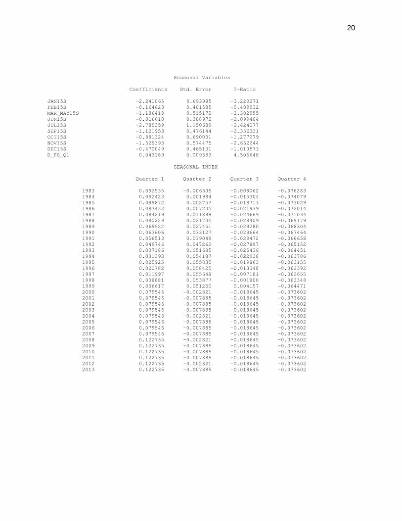
The estimated effects of the seasonal variables are combined into a seasonal index

by multiplying each of the seasonal coefficients by the relevant seasonal variable and

summing across all of the seasonal variables.

This seasonal index can be arrayed by Postal quarter to observe the quarterly

seasonal pattern and to understand how this seasonal pattern changed over time prior

to 2000 as a result of the moving Postal calendar. Since 2000, this seasonal index is

generally constant for a given quarter each year, although changes in the number of

Sundays within a given quarter and the existence of Leap Years lead to some modest

year-to-year changes.

The seasonal coefficients and seasonal index for First-Class Letters, Cards, and

Flats are shown next as an example.

20

Seasonal Variables Coefficients Std. Error T-Ratio JAN15S -2.241065 0.693985 -3.229271 FEB15S -0.164623 0.401585 -0.409932 MAR_MAY15S -1.186418 0.515172 -2.302955 JUN15S -0.816610 0.388972 -2.099404 JUL15S -2.789359 1.150689 -2.424077 SEP15S -1.121953 0.476144 -2.356331 OCT15S -0.881324 0.690001 -1.277279 NOV15S -1.529393 0.574475 -2.662244 DEC15S -0.470049 0.465131 -1.010573 D_FS_Q1 0.043189 0.009583 4.506640 SEASONAL INDEX Quarter 1 Quarter 2 Quarter 3 Quarter 4 1983 0.092535 -0.006505 -0.008062 -0.076283 1984 0.092423 0.001984 -0.015304 -0.074079 1985 0.089872 0.002757 -0.018713 -0.073029 1986 0.087433 0.007205 -0.021979 -0.072014 1987 0.084219 0.011898 -0.024669 -0.071034 1988 0.080229 0.021705 -0.028409 -0.069179 1989 0.069922 0.027451 -0.029280 -0.068304 1990 0.063606 0.033127 -0.029664 -0.067464 1991 0.056513 0.039049 -0.029472 -0.066658 1992 0.049746 0.047262 -0.027897 -0.065152 1993 0.037186 0.051685 -0.025436 -0.064451 1994 0.031393 0.054187 -0.022938 -0.063786 1995 0.025925 0.055835 -0.019863 -0.063155 1996 0.020782 0.058425 -0.013348 -0.062392 1997 0.011997 0.055648 -0.007181 -0.062655 1998 0.008881 0.053877 -0.001800 -0.063348 1999 0.006617 0.051250 0.004157 -0.064471 2000 0.079546 -0.002821 -0.018645 -0.073602 2001 0.079546 -0.007885 -0.018645 -0.073602 2002 0.079546 -0.007885 -0.018645 -0.073602 2003 0.079546 -0.007885 -0.018645 -0.073602 2004 0.079546 -0.002821 -0.018645 -0.073602 2005 0.079546 -0.007885 -0.018645 -0.073602 2006 0.079546 -0.007885 -0.018645 -0.073602 2007 0.079546 -0.007885 -0.018645 -0.073602 2008 0.122735 -0.002821 -0.018645 -0.073602 2009 0.122735 -0.007885 -0.018645 -0.073602 2010 0.122735 -0.007885 -0.018645 -0.073602 2011 0.122735 -0.007885 -0.018645 -0.073602 2012 0.122735 -0.002821 -0.018645 -0.073602 2013 0.122735 -0.007885 -0.018645 -0.073602

21

First-Class Mail First-Class Mail is a heterogeneous class of mail. First-Class Mail includes a wide

variety of mail sent by a wide variety of mailers for a wide variety of purposes. This mail

can be divided into various substreams of mail based on several possible criteria,

including the content of the mail-piece (e.g., bills, statements, advertising, and personal

correspondence), the sender of the mail-piece (e.g., households versus businesses

versus government), or the recipient of the mail-piece (e.g., households versus

business versus government).

First-Class Mail can be broadly divided into two categories of mail: Individual

Correspondence, consisting of household-generated mail and non-household-

generated mail sent a few pieces at a time; and Bulk Transactions, consisting of non-

household-generated mail sent in bulk. Relating these two categories of First-Class

Mail to rate categories, Individual Correspondence mail may be thought of as being

approximately equivalent to First-Class Single-Piece Mail, while Bulk Transactions mail

could be viewed as comparable to First-Class Workshared Mail. Of course, these

equivalences are only approximate.

For econometric estimation purposes, domestic First-Class Mail is divided into three

mail categories: First-Class Single-Piece letters, cards, and flats; First-Class

Workshared letters, cards, and flats; and First-Class Parcels. In addition, a fourth

demand equation is estimated for First-Class International letters, cards, and flats.

22

First-Class Single-Piece Letters, Cards, and Flats

1. Explanatory Variables used in First-Class Single-Piece Letters, Cards, and Flats Equation The First-Class Single-Piece letters, cards, and flats demand equation includes the

following explanatory variables.

(1) Macro-Economic Variables: Employment

The relationship between First-Class Single-Piece letters, cards, and flats, and the

general economy is modeled through the inclusion of Private Employment (EMPLOY)

as an explanatory variable in the First-Class Single-Piece letters, cards, and flats

equation.

Employment was chosen as the macro-economic variable to be included in the First-

Class Single-Piece letters equation on the basis of a comparison of econometric results

including several candidate macro-economic variables, including retail sales,

consumption, and GDP. The theoretical rationale for including total employment as a

macro-economic variable is that in many cases, mail volume is not affected by the dollar

value of economic transactions, so much as by the number of such transactions. For

example, the number of credit card bills one receives does not necessarily go up as the

total amount charged per card goes up. While variables like GDP or retail sales may be

good measures of the total dollar amount of economic activity (e.g., the total amount

charged per credit card), employment appears to be a better measure of the number of

business transactions (e.g., number of credit card bills received).

Employment is filtered using a Hodrick-Prescott filter. The resulting trend

component of Employment (EMPLOY_HPT) is entered into the First-Class Single-Piece

letters, cards, and flats demand equation as an explanatory variable.

23

(2) Postal Prices

The First-Class Single-Piece letters, cards, and flats equation includes a price index

measuring the average price of First-Class Single-Piece letters, cards, and flats

(PX01SP_LCF).

(3) Trends

The First-Class Single-Piece letters, cards, and flats demand equation includes

linear time trends starting at three separate times: 1993Q4, 2002Q4, and 2007Q4.6

The first two of these trends largely reflect changes in the impact of new mail-

diverting technologies which were emerging and being rapidly adopted by businesses

and households during these time periods.

In the 1990s, these technologies were fax, e-mail, and electronic funds transfer

(EFT). In the early 2000s, high-speed Internet was becoming more widely adopted, and

e-mail use began reaching wider audiences. While all of these technologies existed in

limited form for many years, their adoption accelerated over the time periods identified

by these trends.

Given the nature of these trend variables, it is also likely that the changes in the rate

of net mail diversion at these particular times was due to changes in other underlying

trends that might have affected mail volume (some positive, some negative) that may

have been unrelated to the Internet or electronic diversion rates. Trends within

industries which are particularly heavy users of mail – e.g., banking, advertising,

housing – are likely to be picked up by these trends in the same way that more recent

trends in these industries caused by the Great Recession are explained by the more

recent net mail trends that coincided with the Great Recession.

6 These trends appear in the econometric output as “Intervention” variables, where the pulse, step, and attenuation rates of Intervention are constrained to be equal to zero. The result is mathematically identical, then, to including a simple linear time trend starting at the relevant time in the demand equation.

24

The final trend, which starts in 2007Q4, captures changes to long-run trends

associated with the Great Recession. These include, for example, declines in home

ownership and consumers’ use of credit cards due to the Great Recession. Given the

nature of this trend variable, it is also possibly picking up other changes in the rate of

net mail diversion over this time period, which can be positive or negative. For

example, it may include additional electronic diversion due to continuing technological

advances such as changes in payment platforms, or it may reflect a reduction in the rate

of new electronic diversion, as the early and mid-range adopters have converted and

the smaller set of remaining mailers are increasingly less likely to switch.

(4) Other Variables

The First-Class Single-Piece letters, cards, and flats equation includes four dummy

variables: D_R90, which is equal to one since the implementation of R90-1 rates in

February, 1991, zero prior to that; MC95, which is equal to one since the

implementation of classification reform (MC95-1) in July, 1996; R2006PHOP, which is

equal to -1 in 2006Q1 and +1 in 2006Q2 and is related to the Postal Service’s measure

of Postage in the Hands of the Public (PHOP) just before and after the implementation

of R2005-1 rates in January, 2006; and D_R07, which is equal to one since the

implementation of R2006-1 rates in May, 2007, zero earlier.

Finally, the First-Class Single-Piece letters, cards, and flats equation includes a set

of seasonal variables. The seasonal variables in the First-Class Single-Piece letters,

cards, and flats equation include a quarterly dummy for quarter 1 since the introduction

of Forever Stamps in 2007Q3.

25

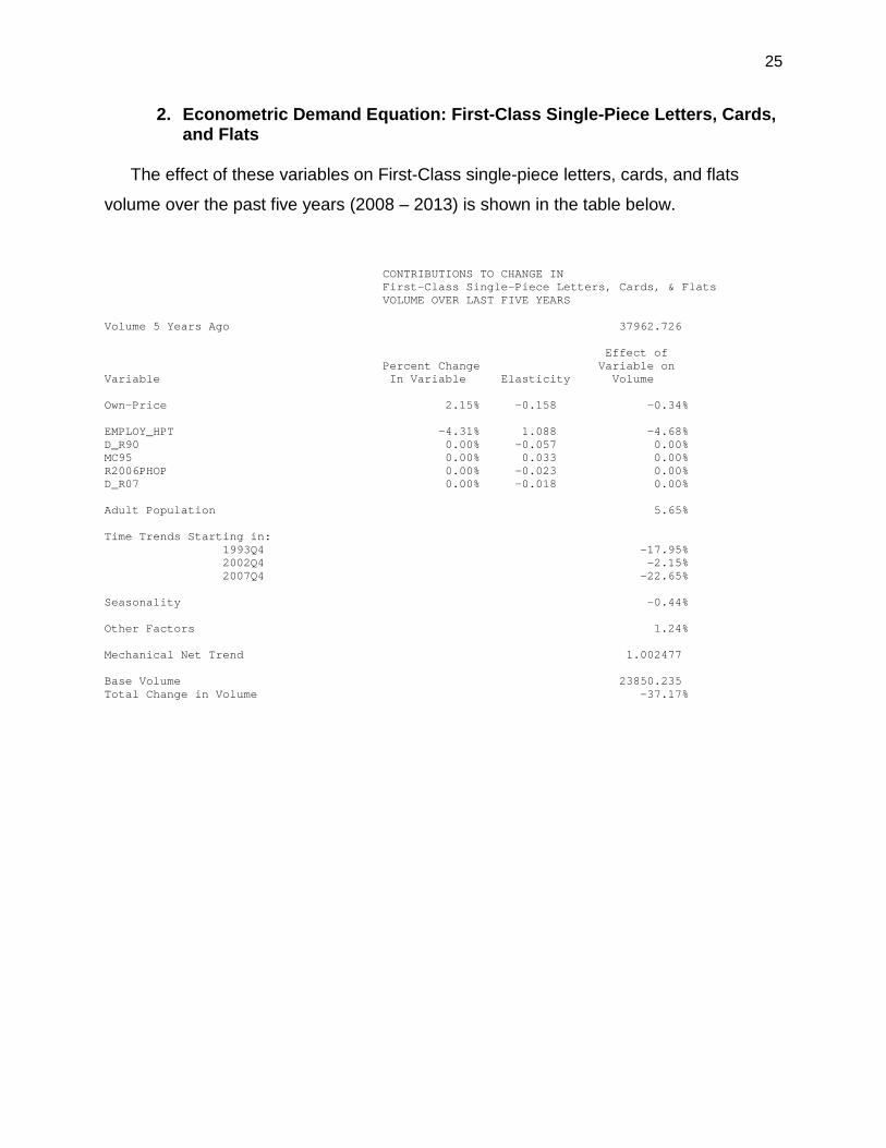
2. Econometric Demand Equation: First-Class Single-Piece Letters, Cards, and Flats

The effect of these variables on First-Class single-piece letters, cards, and flats

volume over the past five years (2008 – 2013) is shown in the table below.

CONTRIBUTIONS TO CHANGE IN First-Class Single-Piece Letters, Cards, & Flats VOLUME OVER LAST FIVE YEARS Volume 5 Years Ago 37962.726 Effect of Percent Change Variable on Variable In Variable Elasticity Volume Own-Price 2.15% -0.158 -0.34% EMPLOY_HPT -4.31% 1.088 -4.68% D_R90 0.00% -0.057 0.00% MC95 0.00% 0.033 0.00% R2006PHOP 0.00% -0.023 0.00% D_R07 0.00% -0.018 0.00% Adult Population 5.65% Time Trends Starting in: 1993Q4 -17.95% 2002Q4 -2.15% 2007Q4 -22.65% Seasonality -0.44% Other Factors 1.24% Mechanical Net Trend 1.002477 Base Volume 23850.235 Total Change in Volume -37.17%

26

First-Class Parcels

1. Explanatory Variables used in First-Class Parcels Equation The First-Class parcels demand equation includes the following explanatory

variables.

(1) Macro-Economic Variables: Mail-Order Retail Sales

First-Class parcel volumes consist largely of the delivery of products bought by the

sender or recipient of the mail so that this type of mail volume derives almost directly

from retail sales. More specifically, First-Class parcels volumes are a function of mail-

order retail sales (which includes e-commerce sales), that is, sales of goods which are

delivered to the consumer.

Hence, the relationship between First-Class parcels and the general economy is

modeled through the inclusion of mail-order Retail Sales (STR_MO) as an explanatory

variable in the First-Class parcels equation.

(2) Time Trends

Unlike most other categories of First-Class Mail, First-Class parcels volume has

been growing fairly strongly in recent years. This is modeled, in part, through the

inclusion of a linear time trend in the First-Class parcels equation, starting in 2011Q3.7

(3) Postal Prices

The First-Class parcels equation includes a price index measuring the average price

of First-Class parcels (PX1_3P).

7 This trend appears in the econometric output as “Intervention” variables, where the pulse, step, and attenuation rates of Intervention are constrained to be equal to zero. The result is mathematically identical, then, to including a simple linear time trend starting at the relevant time in the demand equation.

27

(4) Other Variables

The First-Class parcels equation includes three dummy variables: R2006PHOP,

which is equal to -1 in 2006Q1 and +1 in 2006Q2 and is related to the Postal Service’s

measure of Postage in the Hands of the Public (PHOP) just before and after the

implementation of R2005-1 rates in January, 2006; D2006Q3, which is equal to one in

2006Q3, zero otherwise; and D_R07, which is equal to one since the implementation of

R2006-1 rates in May, 2007 (this rate change introduced shape-based pricing for First-

Class Mail).

Finally, the First-Class parcels equation includes a set of simple quarterly dummies

to model seasonality.

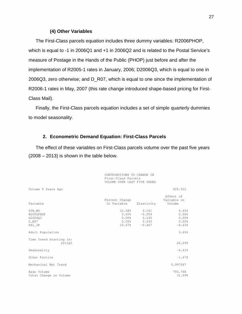
2. Econometric Demand Equation: First-Class Parcels

The effect of these variables on First-Class parcels volume over the past five years

(2008 – 2013) is shown in the table below.

CONTRIBUTIONS TO CHANGE IN First-Class Parcels VOLUME OVER LAST FIVE YEARS Volume 5 Years Ago 605.522 Effect of Percent Change Variable on Variable In Variable Elasticity Volume STR_MO 32.58% 0.161 4.65% R2006PHOP 0.00% -0.059 0.00% D2006Q3 0.00% 0.145 0.00% D_R07 0.00% 0.243 0.00% PX1_3P 10.67% -0.467 -4.63% Adult Population 5.65% Time Trend Starting in: 2011Q3 26.69% Seasonality -0.41% Other Factors -1.47% Mechanical Net Trend 0.997047 Base Volume 793.768 Total Change in Volume 31.09%

28

First-Class Workshared Letters, Cards, and Flats

1. Explanatory Variables used in First-Class Workshared Letters, Cards,

and Flats Equation

The First-Class workshared letters, cards, and flats demand equation includes the

following explanatory variables.

(1) Macro-Economic Variable: Employment

The relationship between First-Class Workshared letters, cards, and flats and the

general economy is modeled through the inclusion of Private Employment (EMPLOY)

as an explanatory variable in the First-Class Workshared letters, cards, and flats

equation.

Employment was chosen as the macro-economic variable to be included in the First-

Class Workshared Mail equation on the basis of a comparison of econometric results

including several candidate macro-economic variables, including retail sales,

consumption, and GDP. The theoretical rationale for including total employment as a

macro-economic variable is that in many cases, mail volume is not affected by the dollar

value of economic transactions, so much as by the number of such transactions. For

example, the number of credit card bills one receives does not necessarily go up as the

total amount charged per card goes up. While variables like GDP or retail sales may be

good measures of the total dollar amount of economic activity (e.g., the total amount

charged per credit card), employment appears to be a better measure of the number of

business transactions (e.g., number of credit card bills received).

Employment is filtered using a Hodrick-Prescott filter. Only the resulting Cyclical

component of Employment (EMPLOY_HPC) is entered into the First-Class Workshared

letters, cards, and flats equation as an explanatory variable, as the Trend Component of

Employment was not found to have a statistically significant impact on First-Class

Workshared mail volume.

29

(2) Postal Prices

The First-Class Workshared letters, cards, and flats equation includes a single

Postal price: the price of First-Class Workshared letters, cards, and flats (PX1WS_LCF).

(3) Logistic Time Trend

The First-Class Workshared letters, cards, and flats equation includes a logistic time

trend starting in 1992Q1 (@LOG(TREND-84)).

This time trend is included in the First-Class Workshared letters, cards, and flats,

demand equation to model positive factors which contributed to First-Class Workshared

mail volume growth through the 1990s and into the 2000s. These factors included

migration of mail from Single-Piece to Workshared mail, positive trends in direct-mail

advertising, and increasing numbers of financial transactions. This time trend is logistic,

which means that it is increasing at a decreasing rate, to reflect the diminishing positive

influence of these factors (particularly shifts of mail from Single-Piece to Workshared)

over time.

(4) Linear Trends

The First-Class Workshared letters, cards, and flats demand equation includes linear

time trends starting at three separate times: 2002Q3, 2004Q1, and 2008Q1.8

The first two of these trends reflect changes in the impact of Internet and electronic

diversion on First-Class Workshared Mail as well as changes in other underlying trends

that might have affected mail volume (some positive, some negative) over these time

periods.

8 These trends appear in the econometric output as “Intervention” variables, where the pulse, step, and attenuation rates of Intervention are constrained to be equal to zero. The result is mathematically identical, then, to including a simple linear time trend starting at the relevant time in the demand equation.

30

The most recent of these trends, which starts in 2008Q1, captures changes to long-

run trends associated with the Great Recession. These include, for example, declines

in home ownership and consumers’ use of credit cards due to the Great Recession.

Given the nature of this trend variable, it is also possibly picking up other changes in the

rate of net mail diversion over this time period, which may be either positive or negative

over this time period.

(5) Other Variables

The First-Class Workshared letters, cards, and flats equation includes one dummy

variables: MC95, which is equal to one since the implementation of MC95-1

classification reform in 1996Q4.

Finally, the First-Class Workshared letters, cards, and flats equation includes a set

of seasonal variables. This includes a dummy variable, D_EL1, which is equal to one in

the first Postal quarter of Federal election years9, to capture election-generated mail

volume such as voter registration cards and candidate literature.

9 The first Postal quarter occurs in the fall preceding the calendar year of the same number, so, for example, 2013Q1 will begin on October 1, 2012. Hence, “the first quarter of Federal election years” refers to the fall (Oct – Dec) of odd-numbered Postal Fiscal Years.

31

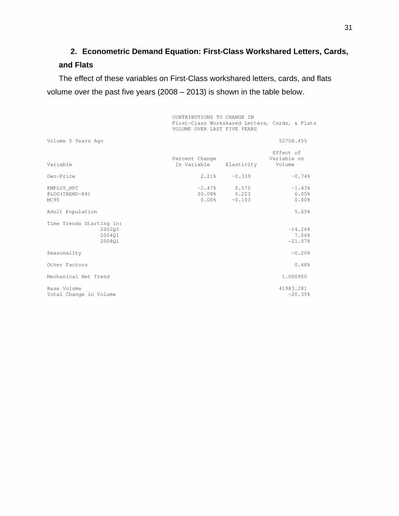
2. Econometric Demand Equation: First-Class Workshared Letters, Cards, and Flats

The effect of these variables on First-Class workshared letters, cards, and flats

volume over the past five years (2008 – 2013) is shown in the table below.

CONTRIBUTIONS TO CHANGE IN First-Class Workshared Letters, Cards, & Flats VOLUME OVER LAST FIVE YEARS Volume 5 Years Ago 52708.455 Effect of Percent Change Variable on Variable In Variable Elasticity Volume Own-Price 2.21% -0.339 -0.74% EMPLOY_HPC -2.47% 0.575 -1.43% @LOG(TREND-84) 30.08% 0.223 6.05% MC95 0.00% -0.103 0.00% Adult Population 5.65% Time Trends Starting in: 2002Q3 -14.26% 2004Q1 7.06% 2008Q1 -21.07% Seasonality -0.20% Other Factors 0.48% Mechanical Net Trend 1.000950 Base Volume 41983.281 Total Change in Volume -20.35%

32

First-Class International Letters, Cards, and Flats

1. Explanatory Variables used in First-Class International Letters, Cards,

and Flats Equation

The First-Class International letters, cards, and flats demand equation includes the

following explanatory variables.

(1) Macro-Economic Variable: Exports

The relationship between First-Class International mail and the general economy is

modeled through the inclusion of real exports per adult (XR) as an explanatory variable

in the First-Class International letters, cards, and flats demand equation.

The theoretical rationale for including exports as a macro-economic variable is that it

is a measure of international economic activity. The assumption is that increased trade

activity would result in an increase in the number of bills, other financial statements, and

other business and personal communications that are mailed to foreign countries.

(2) Time Trend

The First-Class International letters, cards, and flats equation includes a full-sample

linear time trend (TREND).

(3) Postal Prices

The First-Class International letters, cards, and flats equation includes a single

Postal price: the price of First-Class International letters, cards, and flats (PX_LCF).

33

(4) Other Variables

The First-Class International letters, cards, and flats equation includes a dummy

variable, PD09Q1_10Q2, which is equal to one from 2009Q1 through 2010Q2, and is

set equal to zero elsewhere. The First-Class International letters, cards, and flats

equation also includes a set of seasonal variables.

2. Econometric Demand Equation: First-Class International Letters, Cards,

and Flats

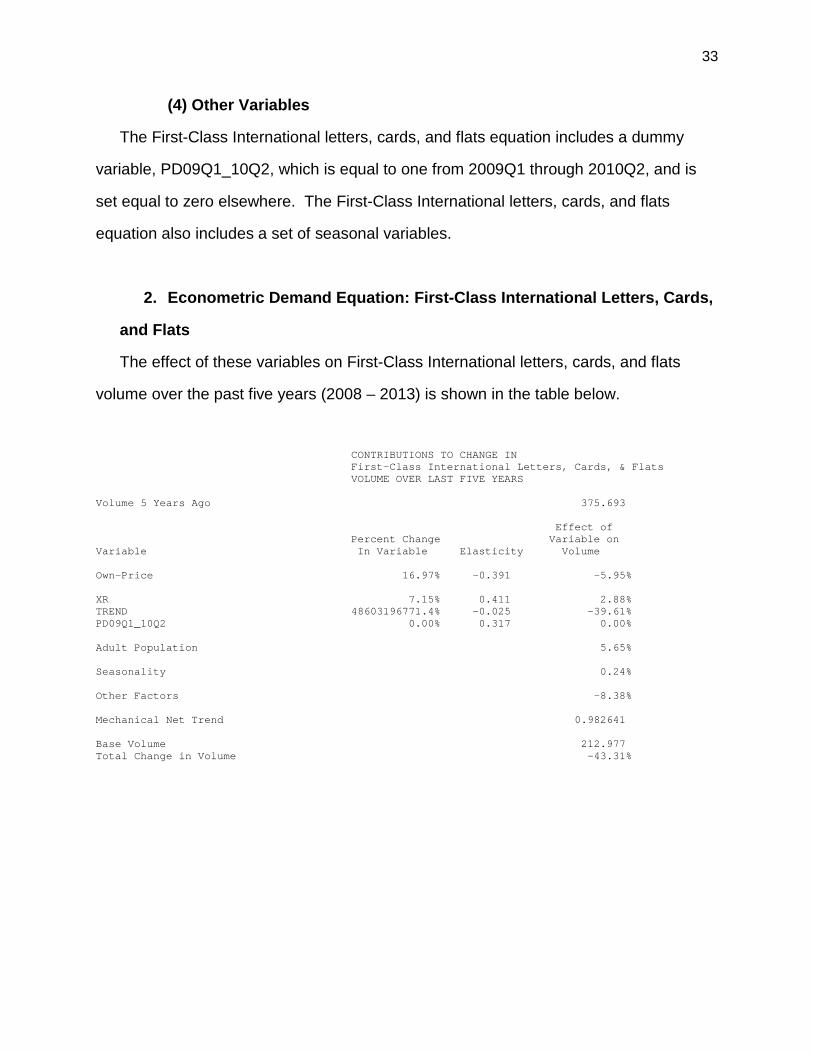
The effect of these variables on First-Class International letters, cards, and flats

volume over the past five years (2008 – 2013) is shown in the table below.

CONTRIBUTIONS TO CHANGE IN First-Class International Letters, Cards, & Flats VOLUME OVER LAST FIVE YEARS Volume 5 Years Ago 375.693 Effect of Percent Change Variable on Variable In Variable Elasticity Volume Own-Price 16.97% -0.391 -5.95% XR 7.15% 0.411 2.88% TREND 48603196771.4% -0.025 -39.61% PD09Q1_10Q2 0.00% 0.317 0.00% Adult Population 5.65% Seasonality 0.24% Other Factors -8.38% Mechanical Net Trend 0.982641 Base Volume 212.977 Total Change in Volume -43.31%

34

Standard Mail

1. Overview of Direct-Mail Advertising

More than 90 percent of Standard Mail can be characterized as direct-mail

advertising. Hence, understanding the demand for direct-mail advertising is the key to

understanding the demand for Standard Mail volume.

The demand for Standard Mail volume is the result of a choice by advertisers

regarding how much to spend on direct-mail advertising expenditures. The decision

process made by direct-mail advertisers can be decomposed into two separate, but

interrelated, decisions:

(1) How much to invest in advertising?

(2) Which advertising medium to use?

These two decisions are integrated into the demand equations associated with

Standard Mail volume by including a set of explanatory variables in the demand

equations for Standard Mail that addresses each of these decisions. These decisions,

and their implications for Standard Mail equations, are considered separately below.

2. Advertising Decisions and Their Impact on Mail Volume

a. How Much to Invest in Advertising

Advertising represents a form of business investment. Hence, the Standard Mail

equations include real gross private domestic investment as a measure of the overall

demand for business investment.

In addition to macroeconomic factors, the overall level of advertising is also affected

by certain other regular events. In particular, in the United States, the election cycle is a

key factor which drives advertising demand. In the case of Standard Mail, the election

cycle is particularly important with respect to preferred-rate mail, i.e., Standard Nonprofit

and Nonprofit Enhanced Carrier Route (ECR) mail. Variables which coincide with the

35

timing of Federal elections are included in the Standard Nonprofit and Nonprofit ECR

demand equations as well as the Standard ECR demand equation.

b. Which Advertising Media to Use

The choice of advertising media can be thought of as primarily a pricing decision, so

that the primary determinant of the demand for direct-mail advertising (vis-à-vis other

advertising media) would be the price of direct-mail advertising.

The most obvious way in which the price of direct-mail advertising is included in the

Standard Mail equations is through the price of Standard Mail. Postage costs are

included in the Standard Mail equations through fixed-weight price indices which

measure the average postage paid by Standard Mailers.

One of the principal advantages of direct-mail advertising over other forms of

advertising is that direct-mail advertising allows an advertiser to address customers on a

one-on-one basis. By identifying specifically who will receive a particular piece of direct-

mail advertising, direct-mail advertising is able to provide an inherent level of targeting

that is not necessarily available through other advertising media.

The ability to target a direct mailing to specific individuals, based on specific

advertiser-chosen criteria, has increased dramatically as a result of technological

advances, particularly over the past fifteen to twenty years. The ease with which one is

able to identify specific consumers or businesses at whom to target direct-mail

advertising is a key component of the cost of direct-mail advertising. A linear time trend

is included in the Standard Regular equation. This time trend has a positive coefficient

through most of the sample period used here, reflecting this positive influence of

targeting.

More recent changes to the overall advertising market as well as direct mail’s role

within that market are modeled via Intervention analysis. The general concept of

Intervention analysis was described earlier in this document. The specific demand

36

specifications associated with the demand equations developed here for Standard Mail

are described below.

The specific demand equations developed for Standard Mail volumes are outlined

next.

37

Standard Regular Mail

1. Explanatory Variables used in Standard Regular Mail Equation

The Standard Regular mail demand equation includes the following explanatory

variables.

(1) Macro-Economic Variable: Investment

The relationship between Standard Regular mail volume and the economy is

modeled through the inclusion of gross private domestic investment (INVR).

(2) Impact of the Great Recession

The Great Recession hit advertising expenditures, and, hence, Standard mail

volume, much harder than would have been expected, even given the decline that

occurred in private investment. To capture this effect econometrically, an Intervention

variable is added to the Standard Regular demand equation that starts in 2008Q2 and

takes the following form:

Ln(Vol)t = a + …+ω0·Pt + ω1·(Pt+δPt-1+δ2Pt-2+δ3Pt-3+…) + ω2·St + …

where Pt is a pulse function and St is a step function, so that Pt = 1 if t=2008Q2 and 0

otherwise; St = 1 if t >2008Q2 and 0 otherwise. This variable has an initial value in

2008Q2 of ω0, which decays toward a long-run value of ω2.

(3) Postal Prices

The Standard Regular mail equation includes a price index measuring the average

price of non-parcel Standard Regular mail (PX3R_N_NP).

38

(4) Time Trend

The Standard Regular mail equation includes a linear trend variable from the start of

the sample period (1988Q1) through 2007Q1, TREND2007Q1. This variable then

maintains a constant level since 2007Q1.

This trend is included to capture general increases in the attractiveness of direct-

mail advertising as a desirable advertising medium as well as in Standard Regular mail

volume specifically relative to other direct-mail alternatives (e.g., Standard ECR mail).

The trend is truncated in 2007 due to weakness in the overall advertising industry

(whose share of GDP declined in both 2006 and 2007 from historical norms) as well as

in specific industries which are heavy users of direct-mail advertising (e.g., the financial

industry) due to the factors which ultimately led to the Great Recession (e.g., housing

prices peaked in 2006).

(5) Other Variables

The Standard Regular mail equation includes several dummy and Intervention

variables to reflect the impact of various one-time events and/or changes to the relative

relationship between Standard Regular mail and other mail categories.

(a) MC95-1

A dummy variable (D1996Q4) equal to one in 1996Q4, zero elsewhere, and an

Intervention variable starting in 1997Q1 are included in the Standard Regular mail

equation to model the impact of classification reform (MC95-1), which was implemented

in the middle of 1996Q4. These variables are included in the Standard Regular demand

equation to reflect the impact of rule changes implemented at that time that are not fully

captured by the Standard Regular price index. The effect of these rule changes in

modeled by an intervention variable instead of a simple dummy to better reflect the fact

that the full impact of mailers to these changes was not necessarily immediate.

39

(b) R97-1

An Intervention variable starting in 1999Q3 is included in the Standard Regular mail

equation to model the impact of R97-1 rates, which were implemented in 1999Q2.

Standard ECR basic letter rates were set greater than Standard Regular automation 5-

digit letter rates in that case, leading some mail to migrate from Standard ECR to

Standard Regular. The effect of this rate crossover is modeled by an intervention

variable instead of a simple dummy to better reflect the fact that it took some mailers

time to adjust their mailing practices to take advantage of the rate savings available to

them from automating their mail.

(c) R2001-1

A dummy variable equal to one starting with the implementation of R2001-1 rates in

2001Q3 (D_R01) is included in the Standard Regular equation to capture volume

changes at this time which are not fully captured by the Standard Regular price index.

(d) 2002Q2

A dummy variable, D2002Q2, is included in the Standard Regular equation, which is

equal to one in 2002Q2, zero elsewhere. This represents the quarter immediately

following a bio-terrorist Anthrax attack in the fall of 2001. This attack had a temporary

negative impact on the level of direct-mail advertising in general and on Standard

Regular mail volumes in particular.

(e) R2006-1

A dummy variable equal to one starting with the implementation of R2006-1 rates in

2007Q3 (D_R07) is included in the Standard Regular equation. Standard ECR

automation letter discounts were eliminated at this time, leading this mail to migrate

from Standard ECR to Standard Regular.

40

(f) 2012

A dummy variable, D2012Q1, equal to one in 2012Q1, zero otherwise, is included in

the Standard Regular equation. Another dummy variable, D2012Q2ON, which is equal

to one from 2012Q2 forward, is also included in the Standard Regular demand

equation. These dummies are included to account for significant unexplained declines

in Standard Regular mail volume in FY 2012 that appear to be permanent.

(g) Election Dummies

Three dummy variables are included in the Standard Regular demand equation to

model the impact of Federal elections on Standard Regular mail volume: D_EL4_PRES,

which is equal to one in the fourth Postal quarter of Presidential election years;

D_EL1_08, which is equal to one in the first Postal quarter of Federal election years

since 2008; and D_EL4_08, which is equal to one in the fourth Postal quarter of Federal

election years since 2008.

(h) Seasonal Variables

Finally, the Standard Regular mail equation includes a set of seasonal variables.

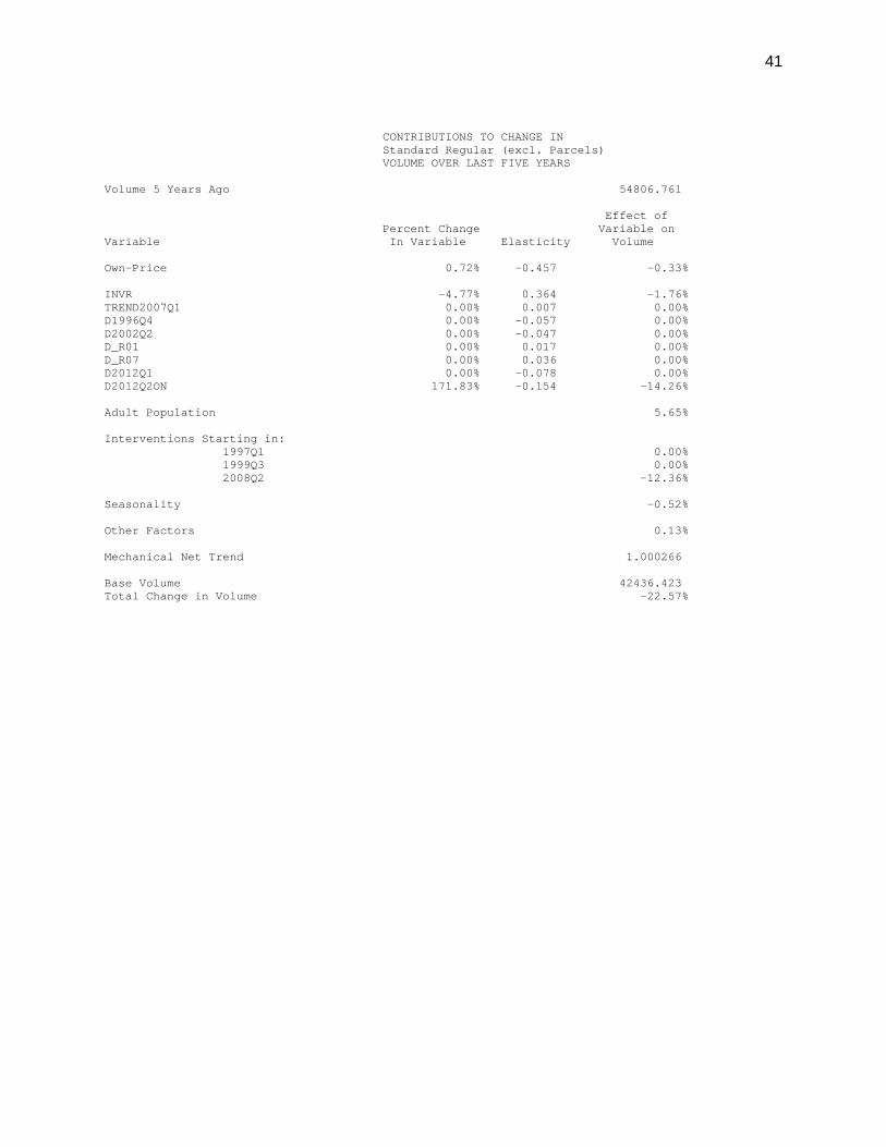
2. Econometric Demand Equation: Standard Regular Mail

The effect of these variables on Standard Regular Mail volume over the past five

years (2008 – 2013) is shown in the table below.

41

CONTRIBUTIONS TO CHANGE IN Standard Regular (excl. Parcels) VOLUME OVER LAST FIVE YEARS Volume 5 Years Ago 54806.761 Effect of Percent Change Variable on Variable In Variable Elasticity Volume Own-Price 0.72% -0.457 -0.33% INVR -4.77% 0.364 -1.76% TREND2007Q1 0.00% 0.007 0.00% D1996Q4 0.00% -0.057 0.00% D2002Q2 0.00% -0.047 0.00% D_R01 0.00% 0.017 0.00% D_R07 0.00% 0.036 0.00% D2012Q1 0.00% -0.078 0.00% D2012Q2ON 171.83% -0.154 -14.26% Adult Population 5.65% Interventions Starting in: 1997Q1 0.00% 1999Q3 0.00% 2008Q2 -12.36% Seasonality -0.52% Other Factors 0.13% Mechanical Net Trend 1.000266 Base Volume 42436.423 Total Change in Volume -22.57%

42

Standard Enhanced Carrier Route Mail

1. Explanatory Variables used in Standard ECR Mail Equation The Standard ECR mail demand equation includes the following explanatory

variables.

(1) Macro-Economic Variable: Investment

The relationship between Standard ECR mail volume and the economy is modeled

through the inclusion of gross private domestic investment per adult (INVR).

(2) Time Trends

The Standard ECR demand equation includes a full-sample time trend (TREND).

The coefficient on TREND is negative, reflecting declining market share for Standard

ECR volume within the general advertising market.

(3) Postal Prices

The Standard ECR mail equation only contains a price index for the price of

Standard ECR mail (PX3R_CR).

(4) Interventions

The Standard ECR mail equation includes two non-linear Interventions to reflect the

impact of changes to the relative relationship between Standard Regular and ECR

prices.

(a) R97-1

With the implementation of R97-1 rates in 1999Q2, Standard ECR basic letter rates

were set greater than Standard Regular automation 5-digit letter rates, leading some

mail to migrate from Standard ECR to Standard Regular.

A non-linear Intervention starting in 1999Q3 is included in the Standard ECR

equation to explain this. This Intervention takes the following form:

43

Ln(Vol)t = a + …+ω0·Pt + ω1·(Pt+δPt-1+δ2Pt-2+δ3Pt-3+…) + ω2·St + …

where Pt is a pulse function and St is a step function, so that Pt = 1 if t=1999Q3 and 0

otherwise; St = 1 if t >1999Q3 and 0 otherwise. This variable has an initial value in

1999Q3 of ω0, which decays toward a long-run value of ω2. A separate dummy variable

for 1999Q2 (the actual quarter in which R97-1 rates took effect), D1999Q2, is also

included in the Standard ECR demand equation.

(b) R2006-1

A second non-linear Intervention variable starting in 2007Q4 is included in the

Standard ECR equation. This coincides with the implementation of R2006-1 rates in

2007Q3 (D_R07). Standard ECR automation letter discounts were eliminated at this

time, leading this mail to migrate from Standard ECR to Standard Regular.

This intervention variable takes the same general form as the R97-1 intervention

variable described above.10

(5) Other Variables

There are two other sets of variables in the Standard ECR mail equation.

(a) Election Dummies

Political campaigns are heavy users of Standard mail volume. Because of the

general timing of Federal elections in only even-numbered years, the effect of elections

on Standard mail volumes is not adequately modeled by simple seasonal variables.

Two such variables are included in the Standard ECR mail equation. The variable

D_EL1_OFF00 has a value of one during the first Postal Quarter of off-year Federal

election years since 2000, and is equal to zero otherwise. The variable D_EL3_OFF is

equal to one in the third quarter of off-year Federal election years

10 Because of the timing and shape of this Intervention variable, it is possible that this variable is also picking up some of the negative influence of the Great Recession on direct-mail advertising and Standard Mail volumes.

44

(b) Seasonal Variables

Finally, the Standard ECR mail equation includes a set of seasonal variables.

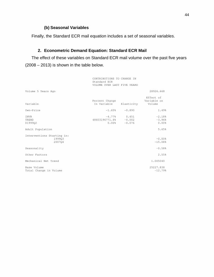
2. Econometric Demand Equation: Standard ECR Mail

The effect of these variables on Standard ECR mail volume over the past five years

(2008 – 2013) is shown in the table below.

CONTRIBUTIONS TO CHANGE IN Standard ECR VOLUME OVER LAST FIVE YEARS Volume 5 Years Ago 28926.668 Effect of Percent Change Variable on Variable In Variable Elasticity Volume Own-Price -1.65% -0.890 1.49% INVR -4.77% 0.451 -2.18% TREND 48603196771.4% -0.002 -3.96% D1999Q2 0.00% -0.076 0.00% Adult Population 5.65% Interventions Starting in: 1999Q3 -0.00% 2007Q4 -15.08% Seasonality -0.58% Other Factors 2.55% Mechanical Net Trend 1.005040 Base Volume 25227.838 Total Change in Volume -12.79%

45

Standard Nonprofit Mail

1. Explanatory Variables used in Standard Nonprofit Mail Equation

The Standard Nonprofit mail demand equation includes the following explanatory

variables.

(1) Macro-Economic Variable: Investment

The relationship between Standard Nonprofit mail volume and the general economy

is modeled through the inclusion of gross private domestic investment per adult (INVR).

Investment is filtered using a Hodrick-Prescott filter. The resulting trend component

of Investment (INVR_HPT) is entered into the Standard Nonprofit equation as an

explanatory variable.

(2) Postal Prices

The Standard Nonprofit mail equation only contains a price index for the price of

Standard Nonprofit mail (PX3N_NCR).

(3) Time Trend

The Standard Nonprofit mail equation includes a full-sample linear time trend,

TREND and a second time trend starting in 2011Q2.11

(4) Interventions

The Standard Nonprofit mail equation includes a non-linear Intervention variable to

model the negative impact of Nonprofit Classification Reform, MC96-1, on Standard

Nonprofit mail volume.

With the implementation of Nonprofit Classification Reform (MC96-1) in October of

1996 (1997Q1), Standard Nonprofit ECR basic letter rates were set greater than

11 The latter of these trends appears in the econometric output as “Intervention” variables, where the pulse, step, and attenuation rates of Intervention are constrained to be equal to zero. The result is mathematically identical, then, to including a simple linear time trend starting at the relevant time in the demand equation.

46

Standard Nonprofit automation 5-digit letter rates, leading some mail to migrate from

Standard Nonprofit ECR to Standard Nonprofit.

A non-linear intervention starting in 1997Q1 is included in the Standard Nonprofit

equation to explain this. This Intervention takes the following form:

Ln(Vol)t = a + …+ω0·Pt + ω1·(Pt+δPt-1+δ2Pt-2+δ3Pt-3+…) + ω2·St + …

where Pt is a pulse function and St is a step function, so that Pt = 1 if t=1997Q1 and 0

otherwise; St = 1 if t >1997Q1 and 0 otherwise. This variable has an initial value in

1997Q1 of ω0, which decays toward a long-run value of ω2.

A second Intervention variable is included in the Standard Nonprofit equation

starting in 2009Q2 to capture the extraordinary impact of the ‘Great Recession’ on

Standard Nonprofit mail volumes. This Intervention variable follows the same

specification as the 1997Q1 Intervention variable, except that the long-run step value,

ω2, is set equal to zero.

(5) Other Variables

There are three other sets of variables in the Standard Nonprofit mail equation.

(a) Election Dummies

Political campaigns are heavy users of Standard mail volume. Because of the

general timing of Federal elections in only even-numbered years, the effect of elections

on Standard mail volumes is not adequately modeled by simple seasonal variables.

Four such variables are included in the Standard Nonprofit mail equation. The

variable D_EL1_OFF has a value of one during Postal Quarter 1 of off-year (i.e., non-

Presidential) Federal election years, and is equal to zero otherwise. The variable

D_EL1_PRES00 has a value of one during the first Postal Quarter of Presidential

election years since 2000 and is equal to zero otherwise. The variable D_EL3_PRES is

equal to one in the third quarter of Presidential Federal election years. The variable

47

D_EL4_PRES96 has a value of one during the fourth Postal quarter of Presidential

election years since 1996, and is equal to zero otherwise.

(b) R2006-1

A dummy variable equal to one starting with the implementation of R2006-1 rates in

2007Q3 (D_R07) is included in the Standard Nonprofit mail equation. Standard

Nonprofit ECR automation letter discounts were eliminated at this time, leading this mail

to migrate from Standard Nonprofit ECR to Standard Nonprofit.

(c) Seasonal Variables

Finally, the Standard Nonprofit mail equation includes a set of seasonal variables.

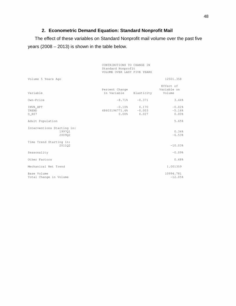
48

2. Econometric Demand Equation: Standard Nonprofit Mail The effect of these variables on Standard Nonprofit mail volume over the past five

years (2008 – 2013) is shown in the table below.

CONTRIBUTIONS TO CHANGE IN Standard Nonprofit VOLUME OVER LAST FIVE YEARS Volume 5 Years Ago 12501.358 Effect of Percent Change Variable on Variable In Variable Elasticity Volume Own-Price -8.71% -0.371 3.44% INVR_HPT -0.10% 0.170 -0.02% TREND 48603196771.4% -0.003 -5.16% D_R07 0.00% 0.027 0.00% Adult Population 5.65% Interventions Starting in: 1997Q1 0.34% 2009Q2 -6.53% Time Trend Starting in: 2011Q2 -10.03% Seasonality -0.09% Other Factors 0.68% Mechanical Net Trend 1.001359 Base Volume 10994.781 Total Change in Volume -12.05%

49

Standard Nonprofit ECR Mail

1. Explanatory Variables used in Standard Nonprofit ECR Mail Equation

The Standard Nonprofit ECR mail demand equation includes the following

explanatory variables.

(1) Macro-Economic Variable: Investment

The relationship between Standard Nonprofit ECR mail volume and the general

economy is modeled through the inclusion of gross private domestic investment per

adult (INVR).

Investment is filtered using a Hodrick-Prescott filter. Only the resulting Cyclical

component of Investment (INVR_HPC) is entered into the Standard Nonprofit ECR

equation as an explanatory variable.

(2) Postal Prices

The Standard Nonprofit ECR mail equation only contains a price index for the price

of Standard Nonprofit ECR mail (PX3N_CR).

(3) Time Trend

The Standard Nonprofit ECR mail equation includes a linear time trend over its full

sample period.

(4) Intervention Variable

The Standard Nonprofit ECR mail equation includes a non-linear Intervention

variable to model the negative impact of Nonprofit Classification Reform, MC96-1, on

Standard Nonprofit ECR mail volume.

With the implementation of Nonprofit Classification Reform (MC96-1) in October of

1996 (1997Q1), Standard Nonprofit ECR basic letter rates were set greater than

50

Standard Nonprofit automation 5-digit letter rates, leading some mail to migrate from

Standard Nonprofit ECR to Standard Nonprofit.

A non-linear intervention starting in 1997Q1 is included in the Standard Nonprofit

ECR equation to explain this. This Intervention takes the following form:

Ln(Vol)t = a + …+ω0·Pt + ω1·(Pt+δPt-1+δ2Pt-2+δ3Pt-3+…) + ω2·St + …

where Pt is a pulse function and St is a step function, so that Pt = 1 if t=1997Q1 and

0 otherwise; St = 1 if t >1997Q1 and 0 otherwise. This variable has an initial value in

1997Q1 of ω0, which decays toward a long-run value of ω2.

(5) Other Variables

There are two additional sets of variables in the Standard Nonprofit ECR mail

equation.

(a) Election Dummies

Political campaigns are heavy users of Standard mail volume. Because of the

general timing of Federal elections in only even-numbered years, the effect of elections

on Standard mail volumes is not adequately modeled by simple seasonal variables.

Three such variables are included in the Standard Nonprofit ECR mail equation.

The variable D_EL1_OFF has a value of one during the first Postal Quarter of off-year

(i.e., non-Presidential) Federal election years, and is equal to zero otherwise. The

variable D_EL4 has a value of one during the fourth Postal Quarter of all Federal

election years (both off-year and Presidential). The variable D_EL1_PRES has a value

of one during the first Postal Quarter of Presidential election years, and is equal to zero

otherwise.

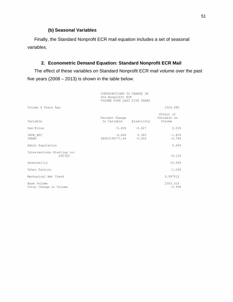
51

(b) Seasonal Variables

Finally, the Standard Nonprofit ECR mail equation includes a set of seasonal

variables.

2. Econometric Demand Equation: Standard Nonprofit ECR Mail

The effect of these variables on Standard Nonprofit ECR mail volume over the past

five years (2008 – 2013) is shown in the table below.

CONTRIBUTIONS TO CHANGE IN Std Nonprofit ECR VOLUME OVER LAST FIVE YEARS Volume 5 Years Ago 2326.480 Effect of Percent Change Variable on Variable In Variable Elasticity Volume Own-Price -5.65% -0.427 2.51% INVR_HPC -4.66% 0.385 -1.82% TREND 48603196771.4% -0.004 -6.78% Adult Population 5.65% Interventions Starting in: 2007Q3 -8.11% Seasonality 10.06% Other Factors -1.24% Mechanical Net Trend 0.997512 Base Volume 2303.516 Total Change in Volume -0.99%

52

Package Delivery Services

Package delivery services refer broadly to the delivery of goods other than

Periodicals, advertisements, and correspondence. Examples of this type of mail include

mail-order deliveries (such as clothes) and the delivery of books, tapes, or CDs (such as

from book or CD clubs), as well as packages sent by households (e.g., Christmas

presents). Among market-dominant mail categories, this encompasses First-Class

Parcels (which were discussed earlier) and the Package Services mail class.

The demand for package delivery services is a derived demand, emanating from the

demand for the products being delivered. As such, the demand for package delivery

services would be expected to be a function of the usual factors affecting demand.

Most Package Delivery Services face significant competition from other delivery

firms, including United Parcel Service and Federal Express. Because of this, most

categories of mail that can best be described as Package Delivery Services are

classified as competitive mail products and are not included as part of this report.

As of January, 2014, there were three market-dominant subclasses of mail in the

Package Services class: Bound Printed Matter, Media Mail, and Library Rate Mail.

Bound Printed Matter refers to any mail that is bound and printed and weighs up to

fifteen pounds. Generally, Bound Printed Matter falls into one of three categories:

catalogs, books (including telephone books in some areas), and direct-mail advertising.

The Media Mail subclass is reserved for books, tapes, and CDs. The Library Rate

subclass is a preferred subclass, generally corresponding to the Media Mail subclass,

available to libraries and certain other institutions. A single demand equation is

estimated for the combined volume of Media Mail and Library Rate mail.

53

The demand for package delivery services will be largely driven by the demand for

the goods being delivered. In the cases of Bound Printed Matter and Media Mail, this

relationship is modeled through the inclusion of mail-order retail sales as an explanatory

variable.

Bound Printed Matter and Media Mail receive somewhat preferred rates from the

Postal Service based on their content. Because of this, these subclasses face less

price-based competition from other package delivery companies than Priority Mail and

Parcel Post. Because of this, competitor prices are not included in the Bound Printed

Matter and Media Mail equations.

The specific demand equations for Bound Printed Matter and Media Mail are

presented in more detail below.

54

Bound Printed Matter

1. Explanatory Variables used in Bound Printed Matter Equation The Bound Printed Matter demand equation includes the following explanatory

variables.

(1) Macro-Economic Variable: Mail-Order Retail Sales

Bound Printed Matter volumes consist largely of catalogs as well as the delivery of

products bought by the sender or recipient of the mail. In both cases, these types of

mail volume can be thought of as deriving almost directly from either expected or actual

retail sales. More specifically, Bound Printed Matter volumes are a function of mail-

order retail sales, that is, sales of goods which are delivered to the consumer. Hence,

mail-order retail sales (which include sales identified as “electronic shopping”, also

referred to as e-commerce) (STR_MO) are included directly in the demand equation for

Bound Printed Matter to reflect this direct relationship between mail-order retail sales

and this mail volume.

(2) Intervention Variable

The Great Recession had a significant negative impact on Bound Printed Matter mail

volume that is not adequately explained by simply including mail-order retail sales

(which did not fall off considerably during the Great Recession).

To capture this effect econometrically, an Intervention variable was added to the

Bound Printed Matter demand equation that starts in 2008Q3 and takes the following

form:

Ln(Vol)t = a + …+ω0·Pt + ω1·(Pt+δPt-1+δ2Pt-2+δ3Pt-3+…) + ω2·St + …

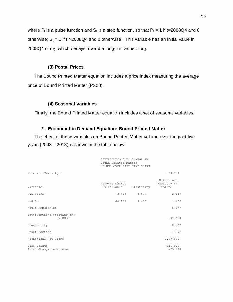
55

where Pt is a pulse function and St is a step function, so that Pt = 1 if t=2008Q4 and 0

otherwise; St = 1 if t >2008Q4 and 0 otherwise. This variable has an initial value in

2008Q4 of ω0, which decays toward a long-run value of ω2.

(3) Postal Prices

The Bound Printed Matter equation includes a price index measuring the average

price of Bound Printed Matter (PX28).

(4) Seasonal Variables

Finally, the Bound Printed Matter equation includes a set of seasonal variables.

2. Econometric Demand Equation: Bound Printed Matter

The effect of these variables on Bound Printed Matter volume over the past five

years (2008 – 2013) is shown in the table below.

CONTRIBUTIONS TO CHANGE IN Bound Printed Matter VOLUME OVER LAST FIVE YEARS Volume 5 Years Ago 598.184 Effect of Percent Change Variable on Variable In Variable Elasticity Volume Own-Price -3.96% -0.638 2.61% STR_MO 32.58% 0.143 4.13% Adult Population 5.65% Interventions Starting in: 2008Q3 -32.60% Seasonality -0.04% Other Factors -1.97% Mechanical Net Trend 0.996039 Base Volume 446.000 Total Change in Volume -25.44%

56

Media and Library Rate Mail

1. Explanatory Variables used in Media and Library Rate Mail Equation The Media and Library Rate Mail demand equation includes the following

explanatory variables.

(1) Macro-Economic Variable: Mail-Order Retail Sales

Media and Library Rate mail volumes consist largely of the delivery of products

bought by the sender or recipient of the mail so that this type of mail volume derives

almost directly from retail sales. More specifically, Media and Library Rate mail

volumes are a function of mail-order retail sales, that is, sales of goods which are

delivered to the consumer. Hence, mail-order retail sales (which include sales identified

as “electronic shopping” , also referred to as e-commerce) (STR_MO) are included

directly in the demand equation for Media and Library Rate Mail to reflect this direct

relationship between mail-order retail sales and this mail volume. Mail-order retail sales

are lagged two quarters in the Media and Library Rate mail demand equation.

(2) Trends

While e-commerce, which is a growing component of mail-order retail sales, has had

a positive impact on Media and Library Rate mail volume, the Internet has also had an

offsetting negative impact on Media mail volume by providing an alternative delivery

source for such items as music, videos, and computer software. This negative impact

has increased with the increasing availability of higher-speed Internet connections

which have made it quicker and easier to download these types of things instead of

having them delivered through the mail.

57

The Media and Library Rate mail demand equation includes two linear time trends to

model this negative diversion, starting in 1996Q4 and 2010Q1.12 The latter of these

trends is likely also picking up ongoing negative influences of the Great Recession on

Media and Library Rate mail volumes.

(3) Postal Prices

The Media and Library Rate mail equation includes the price of Media and Library

Rate Mail (PX29_30).

(4) Intervention

The Media and Library Rate mail demand equation includes one non-linear

Intervention to model a sudden unexplained decline in Media and Library Rate mail

volume in 2001. This intervention variable begins in 2000Q4 and takes the form:

Ln(Vol)t = a + … +ω0·Pt + ω1·(Pt+δPt-1+δ2Pt-2+δ3Pt-3+…) + …

where Pt is a pulse function equal to one in the initial period of the Intervention and zero

otherwise. These variables have initial values, then, of ω0 (separate values for ω0, ω1,

and δ are estimated for each Intervention), which decay toward a long-run value of zero.

The Media and Library Rate mail demand equation also includes one dummy

variable, D1998Q2, which is equal to one in 1998Q2, and zero elsewhere.

(5) Seasonal Variables

Finally, the Media and Library Rate Mail equation includes a set of seasonal

variables.

12 These trends appear in the econometric output as “Intervention” variables, where the pulse, step, and attenuation rates of Intervention are constrained to be equal to zero. The result is mathematically identical, then, to including a simple linear time trend starting at the relevant time in the demand equation.

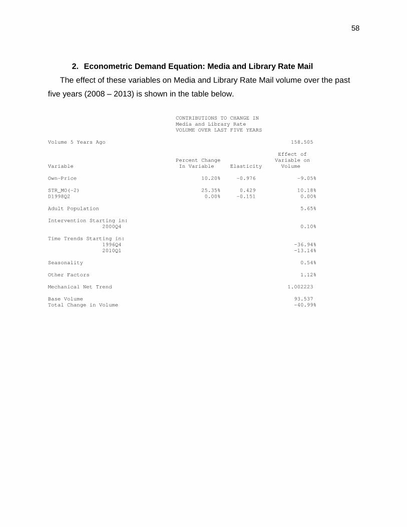
58

2. Econometric Demand Equation: Media and Library Rate Mail

The effect of these variables on Media and Library Rate Mail volume over the past

five years (2008 – 2013) is shown in the table below. CONTRIBUTIONS TO CHANGE IN Media and Library Rate VOLUME OVER LAST FIVE YEARS Volume 5 Years Ago 158.505 Effect of Percent Change Variable on Variable In Variable Elasticity Volume Own-Price 10.20% -0.976 -9.05% STR_MO(-2) 25.35% 0.429 10.18% D1998Q2 0.00% -0.151 0.00% Adult Population 5.65% Intervention Starting in: 2000Q4 0.10% Time Trends Starting in: 1996Q4 -36.94% 2010Q1 -13.14% Seasonality 0.54% Other Factors 1.12% Mechanical Net Trend 1.002223 Base Volume 93.537 Total Change in Volume -40.99%

59

Periodicals Mail The Periodicals Mail class is available for mail that is sent at regular intervals and

contains at least a minimum level of editorial (i.e., non-advertising) content. This

type of mail may include magazines, newspapers, journals, and newsletters. The

Periodicals Mail class is divided into four subclasses, Periodicals Regular and three

subclasses which offer preferred rates for certain eligible mailers. Periodicals

Within-County mail is open to Periodicals which are sent within the same county as

they are printed. Periodicals Nonprofit mail is open to Periodicals sent by qualified

not-for-profit organizations. Periodicals Classroom mail is open to Periodicals sent

to educational institutions for educational purposes.

1. Factors Affecting Demand for Periodicals Mail

The demand for Periodicals mail is a derived demand, which is derived from the

demand of consumers for magazines and newspapers. Those factors which

influence the demand for newspapers and magazines would therefore be expected

to be the principal drivers of the demand for Periodicals mail.

The factors which would be expected to influence the demand for newspapers and

magazines are drawn from basic micro-economic theory. These factors include the

state of the overall economy, the price of periodicals, and the demand for goods which

may serve as substitutes for newspapers and magazines.

The Periodicals demand equation includes total private employment. Employment

worked better econometrically at explaining Periodicals mail volumes than other macro-

economic variables tested, including personal disposable income, consumption

expenditures, and retail sales.

The price of periodicals is measured by the price of postage paid by publishers (and

paid implicitly by consumers through subscription rates). In addition to affecting the

price of newspapers and magazines by being incorporated into subscription rates, the

60

price charged by the Postal Service will also affect the demand for Periodicals mail

directly by affecting publishers’ decisions over how to deliver their Periodicals. For

example, the delivery requirements of many weekly newspapers can be satisfied by

either mail or private delivery.

The Periodicals demand equations used here also includes a long-run time trend.

This long-run trend is the result of long-run demographic shifts away from reading. In

addition to the full-sample linear time trend, two additional negative trends are also

included in the Periodicals demand equation to account for more recent declines in

Periodicals Mail volume due to the Great Recession as well as increased substitution

faced by Periodicals from the Internet.

A single demand equation is estimated for total Periodicals Mail.

2. Explanatory Variables Used in Periodicals Mail Equation

The Periodicals Mail demand equation includes the following explanatory variables.

(1) Macro-Economic Variable: Employment

The relationship between Periodicals Mail and the general economy is modeled

through the inclusion of Private Employment (EMPLOY) as an explanatory variable in

the Periodicals Mail equation.

Employment is filtered using a Hodrick-Prescott filter. The resulting trend and

cyclical components of Employment (EMPLOY_HPT and EMPLOY_HPC, respectively)

are included as explanatory variables in the Periodicals Mail demand equation, with the

latter (EMPLOY_HPC) lagged one quarter.

(3) Time Trends

Periodicals volumes have been in decline for the past twenty years or more. This is

due, in large part, to demographic shifts away from reading toward other activities,

including television. These long-run negative trends in Periodicals volumes are

61

modeled econometrically through a time trend starting in 1993Q2 (the second quarter of

the sample period).

The negative trends in Periodicals Mail volume accelerated significantly as a result

of the Great Recession. To model this impact of the Great Recession, a second time

trend is added to the Periodicals Mail equation starting in 2008Q2. A third time trend

starts in 2011Q2 to capture a further increase in the negative trend in Periodicals Mail

volume at that time.13

(4) Postal Prices

The Periodicals Mail demand equation includes a price index measuring the average

price of Periodicals Mail (PX2C).

(5) Seasonal Variables

Finally, the Periodicals Mail equation includes a set of seasonal variables.

13 These trends appear in the econometric output as “Intervention” variables, where the pulse, step, and attenuation rates of Intervention are constrained to be equal to zero. The result is mathematically identical, then, to including a simple linear time trend starting at the relevant time in the demand equation.

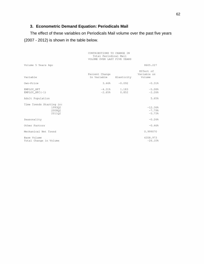
62

3. Econometric Demand Equation: Periodicals Mail The effect of these variables on Periodicals Mail volume over the past five years

(2007 - 2012) is shown in the table below.

CONTRIBUTIONS TO CHANGE IN Total Periodical Mail VOLUME OVER LAST FIVE YEARS Volume 5 Years Ago 8605.227 Effect of Percent Change Variable on Variable In Variable Elasticity Volume Own-Price 3.46% -0.092 -0.31% EMPLOY_HPT -4.31% 1.183 -5.08% EMPLOY_HPC(-1) -2.65% 0.852 -2.26% Adult Population 5.65% Time Trends Starting in: 1993Q2 -12.36% 2008Q2 -7.79% 2011Q2 -5.73% Seasonality -0.26% Other Factors -0.46% Mechanical Net Trend 0.999070 Base Volume 6358.973 Total Change in Volume -26.10%

63

Free Mail Services

There are two mail categories for which mail is free to the sender: Postal Penalty

Mail, mail sent by the Postal Service, and Free-for-the-Blind Mail, which is free for blind

or handicapped consumers. Because these mail categories are free, Postal prices are

not included as explanatory variables in these equations. The specific demand

equations used to model Postal Penalty and Free-for-the-Blind mail volumes are

outlined below.

Postal Penalty Mail

The Postal Penalty mail demand equation includes the following explanatory

variables.

(1) Time Trend

The Postal Penalty equation includes a linear time trend, TREND.

(2) Dummy Variables

The Postal Penalty equation includes two dummy variables, D2013Q1 and

D2013Q4, which are equal to one in 2013Q1 and 2013Q4, respectively, zero

elsewhere.

(3) Seasonal Variables

Finally, the Postal Penalty mail equation includes a set of seasonal variables.

Free-for-the-Blind and Handicapped Mail

The Free-for-the-Blind Mail demand equation includes the following explanatory

variables.

(1) Time Trend

The Free-for-the-Blind demand equation includes a linear time trend, TREND.

(2) Seasonal Variables

Finally, the Free-for-the-Blind Mail equation includes a set of simple quarterly

dummy variables to model seasonality.

64

Special Services

1. General Overview

Except for Money Orders and Post Office Boxes, special services are not mail

volumes, but represent add-ons to mail volumes. That is, a certified letter would be

counted as both a piece of Certified Mail as well as a First-Class letter. Therefore, the

volumes of special services are not included in a calculation of total Postal Service

volume.

Because special services are add-ons to existing mail volumes, the demand for

special services may be affected directly by the demand for complementary categories

of mail. For example, the volume of Stamped Envelopes is modeled in part as a

function of the volume of First-Class Single-Piece Letters since all Stamped Envelopes

are, in fact, First-Class Single-Piece Letters.

In addition, the special service volumes modeled here have generally exhibited long-

run trends. For this reason, a time trend is included in the demand equation associated

with most of the special services.

Finally, of course, the demand for special service mail is also a function of the price

charged by the Postal Service for these services. In addition, most of the special

service equations also include some equation-specific variables, which are described

below.

Specific demand equations for special services are described in detail below.

65

Registered Mail

1. Explanatory Variables used in Registered Mail Equation

The Registered Mail demand equation includes the following explanatory variables.

(1) Macro-Economic Variable: Employment

The relationship between Registered Mail and the general economy is modeled

through the inclusion of Private Employment (EMPLOY) as an explanatory variable in

the Registered Mail equation.

Employment is filtered using a Hodrick-Prescott filter. The resulting trend and

cyclical components of Employment (EMPLOY_HPT and EMPLOY_HPC, respectively)

were experimented with as separate explanatory variables in the Registered Mail

equation. Based on these experiments, Registered Mail volume was found to only be a

function of the cyclical component of Employment (EMPLOY_HPC). Therefore, only

EMPLOY_HPC is included in the Registered Mail demand equation.

(2) Time Trend

The Registered Mail equation includes two time trends to account for the long-run

decline which is the predominant feature of Registered Mail volume: a full-sample linear

time trend, TREND, and a second time trend starting in 2001Q3.14

(3) Postal Prices

The Registered Mail equation includes a price index measuring the average price of

Registered Mail (PX35).

14 The latter of these trends appear in the econometric output as an “Intervention” variable, where the pulse, step, and attenuation rates of Intervention are constrained to be equal to zero. The result is mathematically identical to including a simple linear time trend starting at the relevant time in the demand equation.

66

(4) Dummy Variables

The Registered Mail equation contains three dummy variables: D98Q1, D2002Q1,

and D2007Q2. The first of these, D98Q1, is equal to zero through 1997Q4 and is equal

to one thereafter. Prior to 1998, Registered Mail volume as reported by the Postal

Service’s RPW system included both domestic and international Registered Mail.

Starting in 1998Q1, however, domestic and international Registered Mail volumes were

reported separately. The Registered Mail demand equation described here uses

domestic Registered Mail as its dependent variable since 1998Q1. The dummy D98Q1

accounts for the inclusion of international Registered Mail before that time.

The latter two dummy variables, D2002Q1 and D2007Q2, are equal to one in

2002Q1 and 2007Q2, respectively, and zero elsewhere. The first of these variables is

included to measure the impact of 9/11 and the bioterrorist attack in the autumn of 2001

on Registered Mail volume. The latter variable is simply included because Registered

Mail volume in 2007Q2 is something of an outlier.

(5) Seasonal Variables

Finally, the Registered Mail equation includes a set of seasonal variables. These

seasonal variables include dummy variables for Postal quarters 1 and 3 since the

introduction of the Forever Stamp in 2007Q3.

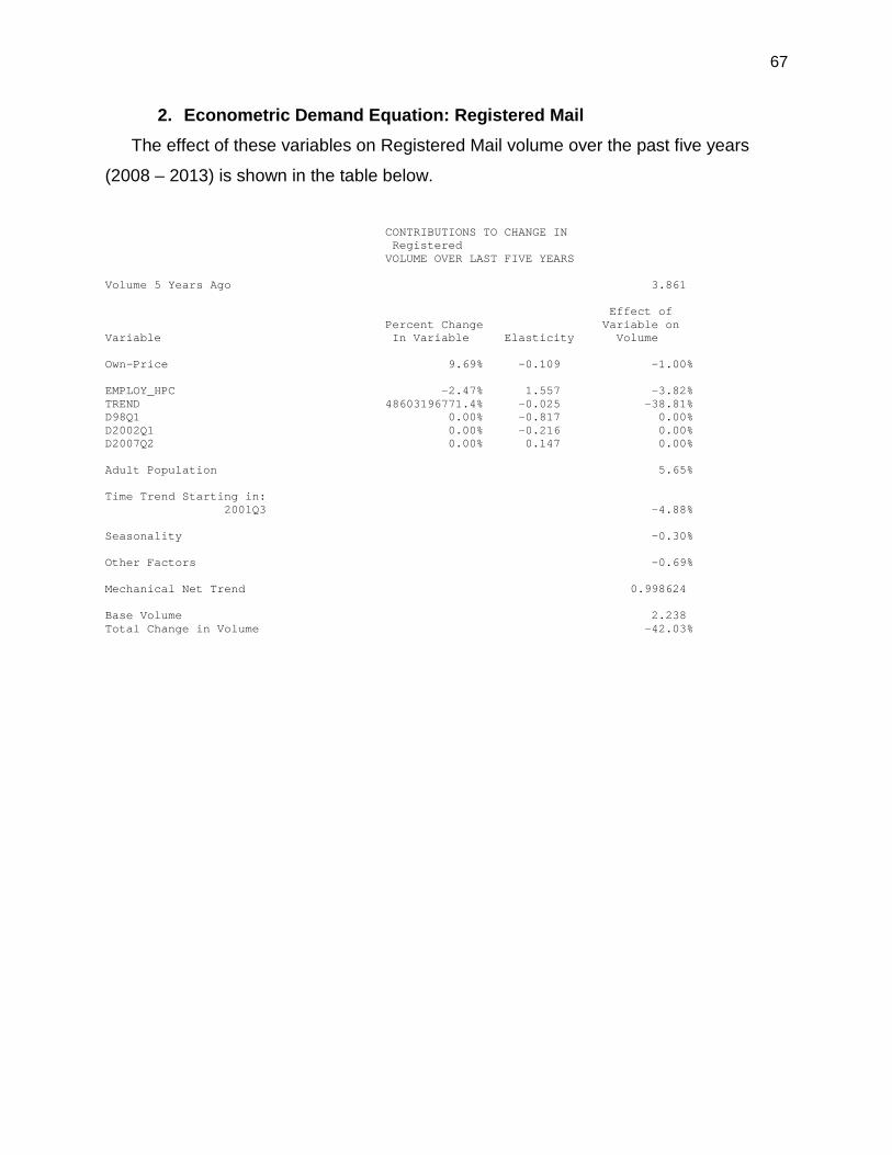
67

2. Econometric Demand Equation: Registered Mail The effect of these variables on Registered Mail volume over the past five years

(2008 – 2013) is shown in the table below.

CONTRIBUTIONS TO CHANGE IN Registered VOLUME OVER LAST FIVE YEARS Volume 5 Years Ago 3.861 Effect of Percent Change Variable on Variable In Variable Elasticity Volume Own-Price 9.69% -0.109 -1.00% EMPLOY_HPC -2.47% 1.557 -3.82% TREND 48603196771.4% -0.025 -38.81% D98Q1 0.00% -0.817 0.00% D2002Q1 0.00% -0.216 0.00% D2007Q2 0.00% 0.147 0.00% Adult Population 5.65% Time Trend Starting in: 2001Q3 -4.88% Seasonality -0.30% Other Factors -0.69% Mechanical Net Trend 0.998624 Base Volume 2.238 Total Change in Volume -42.03%

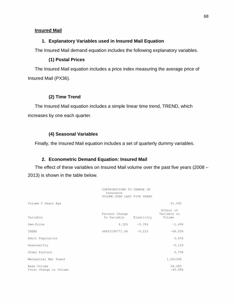
68

Insured Mail

1. Explanatory Variables used in Insured Mail Equation

The Insured Mail demand equation includes the following explanatory variables.

(1) Postal Prices

The Insured Mail equation includes a price index measuring the average price of

Insured Mail (PX36).

(2) Time Trend

The Insured Mail equation includes a simple linear time trend, TREND, which

increases by one each quarter.

(4) Seasonal Variables

Finally, the Insured Mail equation includes a set of quarterly dummy variables.

2. Econometric Demand Equation: Insured Mail

The effect of these variables on Insured Mail volume over the past five years (2008 –

2013) is shown in the table below. CONTRIBUTIONS TO CHANGE IN Insurance VOLUME OVER LAST FIVE YEARS Volume 5 Years Ago 51.595 Effect of Percent Change Variable on Variable In Variable Elasticity Volume Own-Price 4.32% -0.354 -1.49% TREND 48603196771.4% -0.033 -48.05% Adult Population 5.65% Seasonality -0.12% Other Factors 0.79% Mechanical Net Trend 1.001568 Base Volume 28.080 Total Change in Volume -45.58%

69

Certified Mail

1. Explanatory Variables used in Certified Mail Equation

The Certified Mail demand equation includes the following explanatory variables.

(1) Postal Prices

The Certified Mail equation includes a price index measuring the average price of

Certified Mail (PX37).

(2) Intervention Variable

The Certified Mail equation includes an Intervention variable that starts in 2011Q1 to

model significant declines in Certified Mail volume that started around this time. This

variable takes the following form:

Ln(Vol)t = a + …+ω0·Pt + ω1·(Pt+δPt-1+δ2Pt-2+δ3Pt-3+…) + ω2·St + …

where Pt is a pulse function and St is a step function, so that Pt = 1 if t=2011Q1 and 0

otherwise; St = 1 if t >2011Q1 and 0 otherwise. This variable has an initial value in

2008Q2 of ω0, which decays toward a long-run value of ω2.

(3) Other Variables

Finally, the Certified Mail equation includes a set of quarterly dummy variables.

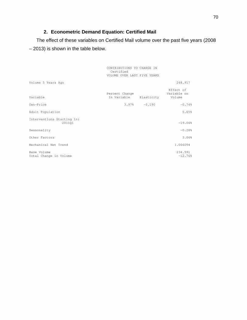
70

2. Econometric Demand Equation: Certified Mail The effect of these variables on Certified Mail volume over the past five years (2008

– 2013) is shown in the table below.

CONTRIBUTIONS TO CHANGE IN Certified VOLUME OVER LAST FIVE YEARS Volume 5 Years Ago 268.917 Effect of Percent Change Variable on Variable In Variable Elasticity Volume Own-Price 3.97% -0.190 -0.74% Adult Population 5.65% Interventions Starting in: 2011Q1 -19.06% Seasonality -0.28% Other Factors 3.06% Mechanical Net Trend 1.006054 Base Volume 234.591 Total Change in Volume -12.76%

71

Collect-on-Delivery Mail

1. Explanatory Variables used in COD Mail Equation

The COD Mail demand equation includes the following explanatory variables.

(1) Retail Package Volumes

COD Mail volume is not stand-alone mail, but instead is an add-on to other types of

mail. Generally, the type of mail that might be sent via COD is retail package mail.

Retail package volume (BGVOL_PKG) (which is equal to the sum of the volumes of

Priority Mail, Retail Parcel Post, and Media Mail (all per adult per Postal delivery day)),

is included as an explanatory variable in the COD Mail equation.

(2) Time Trends

The COD Mail demand equation includes a linear time trend (TREND) to explain the

persistent negative long-run trend in COD volume.

(3) Other Variables

Finally, the COD Mail equation includes dummy variables equal to one in 2005Q1

(D2005Q1) and 2005Q2 (D2005Q2), zero elsewhere, and a set of quarterly dummy

variables.

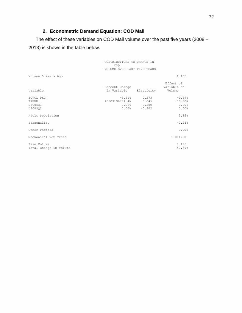
72

2. Econometric Demand Equation: COD Mail The effect of these variables on COD Mail volume over the past five years (2008 –

2013) is shown in the table below. CONTRIBUTIONS TO CHANGE IN COD VOLUME OVER LAST FIVE YEARS Volume 5 Years Ago 1.155 Effect of Percent Change Variable on Variable In Variable Elasticity Volume BGVOL_PKG -9.51% 0.273 -2.69% TREND 48603196771.4% -0.045 -59.30% D2005Q1 0.00% -0.200 0.00% D2005Q2 0.00% -0.202 0.00% Adult Population 5.65% Seasonality -0.24% Other Factors 0.90% Mechanical Net Trend 1.001790 Base Volume 0.486 Total Change in Volume -57.89%

73

Money Orders

1. Explanatory Variables used in Money Orders Equation

The Money Orders demand equation includes the following explanatory variables.

(1) Macro-Economic Variable: Employment

The relationship between Money Orders volume and the general economy is

modeled by including private Employment (EMPLOY) in the Money Orders demand

equation. Employment is filtered using a Hodrick-Prescott filter. The trend and cyclical

components of Employment (EMPLOY_HPT, EMPLOY_HPC) are then entered into the

Money Orders demand equation as separate explanatory variables.

(2) Time Trends

Money Orders volume has been down significantly and consistently since late 2000.

The likely cause of this downturn is increasing competition from electronic alternatives,

such as pre-paid debit cards, as well as from alternate suppliers of money orders.

Long-run trends in Money Orders volume also appear to have been affected by the

Great Recession.

To account for these factors, the Money Orders equation includes linear time trends

starting in 1996Q4, 2003Q1, and 2009Q1.15

(3) Postal Prices

The Money Orders equation includes a price index measuring the average price of

Money Orders (PX39).

15 These trends appear in the econometric output as “Intervention” variables, where the pulse, step, and attenuation rates of Intervention are constrained to be equal to zero. The result is mathematically identical, then, to including a simple linear time trend starting at the relevant time in the demand equation.

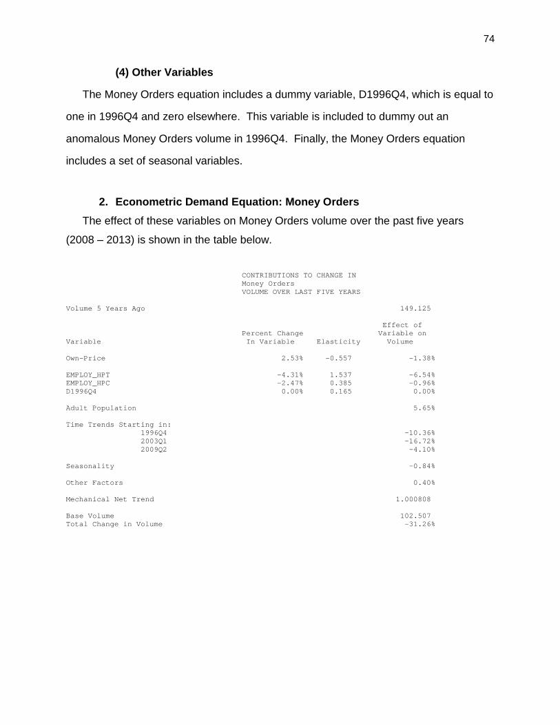
74

(4) Other Variables

The Money Orders equation includes a dummy variable, D1996Q4, which is equal to

one in 1996Q4 and zero elsewhere. This variable is included to dummy out an

anomalous Money Orders volume in 1996Q4. Finally, the Money Orders equation

includes a set of seasonal variables.

2. Econometric Demand Equation: Money Orders

The effect of these variables on Money Orders volume over the past five years

(2008 – 2013) is shown in the table below.

CONTRIBUTIONS TO CHANGE IN Money Orders VOLUME OVER LAST FIVE YEARS Volume 5 Years Ago 149.125 Effect of Percent Change Variable on Variable In Variable Elasticity Volume Own-Price 2.53% -0.557 -1.38% EMPLOY_HPT -4.31% 1.537 -6.54% EMPLOY_HPC -2.47% 0.385 -0.96% D1996Q4 0.00% 0.165 0.00% Adult Population 5.65% Time Trends Starting in: 1996Q4 -10.36% 2003Q1 -16.72% 2009Q2 -4.10% Seasonality -0.84% Other Factors 0.40% Mechanical Net Trend 1.000808 Base Volume 102.507 Total Change in Volume -31.26%

75

Return Receipts

1. Explanatory Variables used in Return Receipts Equation

The Return Receipts demand equation includes the following explanatory variables.

(1) Certified Mail Volume

Return Receipts must be attached to Express Mail or one of Certified, Insured, or

COD Mail. The vast majority of Return Receipts are attached to Certified Mail.

Because of this, the Return Receipts demand equation includes the volume of Certified

Mail (BGVOL37) as an explanatory variable.

(2) Postal Prices

The Return Receipts demand equation includes a price index measuring the

average price of Return Receipts (PX_RR).

(3) Time Trend

The Return Receipts demand equation includes a linear time trend estimated

starting in 2007Q1.16

(4) Dummy Variables

The Return Receipts demand equation includes four dummy variables: D_MEPS,

D1995Q2, D1997Q2, and D_R07. The first of these, D_MEPS, is equal to zero through

1995Q1 and is equal to one from 1995Q2 forward. There was a change in the RPW

system of reporting volumes in 1995Q2, with the new system being called MEPS (Mail

Exit-Point System). Possibly because of this, there was a significant increase in the

reported volume of Return Receipts after 1995Q2 as compared to before 1995Q2. This

is accounted for by the inclusion of D_MEPS in the Return Receipts demand equation. 16 This trend appears in the econometric output as “Intervention” variables, where the pulse, step, and attenuation rates of Intervention are constrained to be equal to zero. The result is mathematically identical, then, to including a simple linear time trend starting at the relevant time in the demand equation.

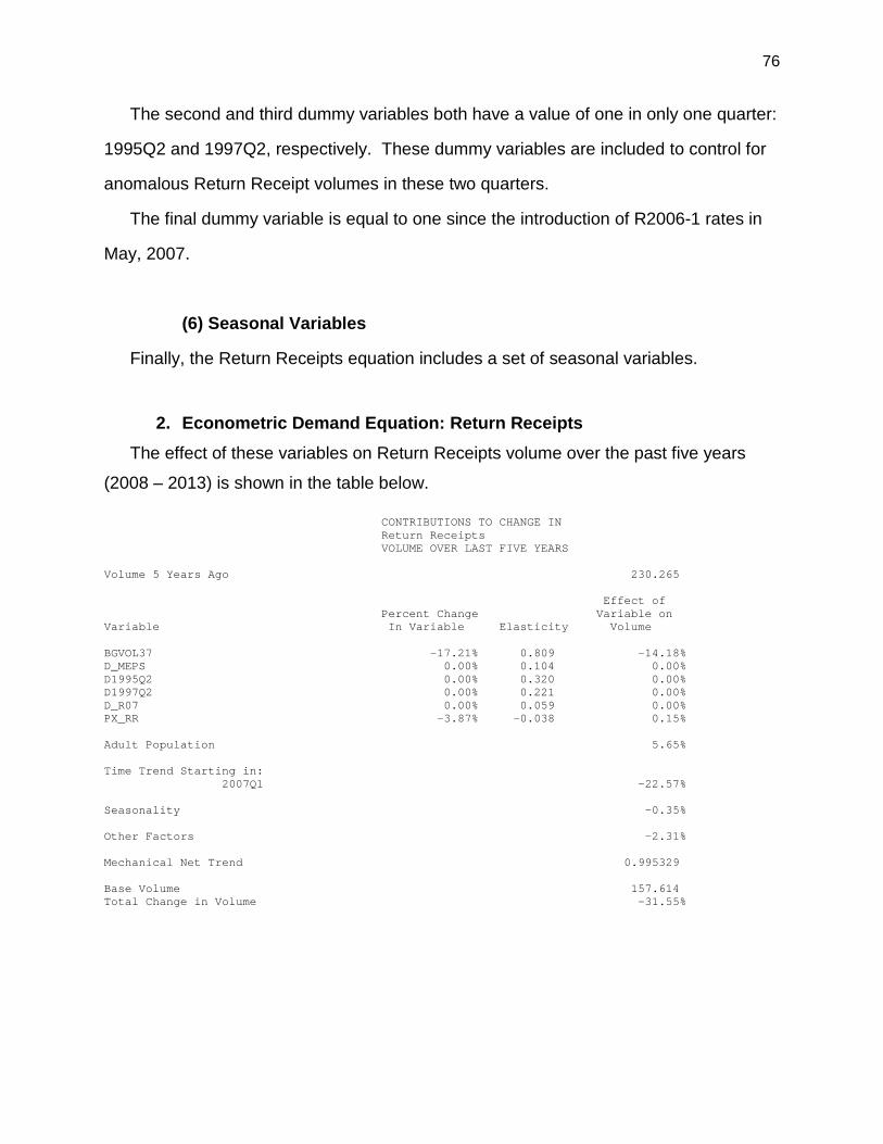
76

The second and third dummy variables both have a value of one in only one quarter:

1995Q2 and 1997Q2, respectively. These dummy variables are included to control for

anomalous Return Receipt volumes in these two quarters.

The final dummy variable is equal to one since the introduction of R2006-1 rates in

May, 2007.

(6) Seasonal Variables

Finally, the Return Receipts equation includes a set of seasonal variables.

2. Econometric Demand Equation: Return Receipts

The effect of these variables on Return Receipts volume over the past five years

(2008 – 2013) is shown in the table below. CONTRIBUTIONS TO CHANGE IN Return Receipts VOLUME OVER LAST FIVE YEARS Volume 5 Years Ago 230.265 Effect of Percent Change Variable on Variable In Variable Elasticity Volume BGVOL37 -17.21% 0.809 -14.18% D_MEPS 0.00% 0.104 0.00% D1995Q2 0.00% 0.320 0.00% D1997Q2 0.00% 0.221 0.00% D_R07 0.00% 0.059 0.00% PX_RR -3.87% -0.038 0.15% Adult Population 5.65% Time Trend Starting in: 2007Q1 -22.57% Seasonality -0.35% Other Factors -2.31% Mechanical Net Trend 0.995329 Base Volume 157.614 Total Change in Volume -31.55%

77

Post Office Boxes

1. Explanatory Variables used in Post Office Boxes Equation

The Post Office Boxes demand equation includes the following explanatory

variables.

(1) Macro-Economic Variable: Employment

The relationship between Post Office Boxes and the macro-economy is modeled by

including total private employment per adult (EMPLOY).

Employment is filtered using a Hodrick-Prescott filter. The resulting trend

component of Employment (EMPLOY_HPT) is entered into the Post Office Box demand

equation as an explanatory variable.

(2) Postal Prices

The Post Office Box equation includes a price index measuring the average price of

Post Office Boxes (PX_PO).

(3) Dummy Variables

Dummy variables equal to one in 2008Q1 (D2008Q1) and 2012Q2 (D2012Q2), and

zero elsewhere, are included in the Post Office Boxes equation, as well as D_R12,

which is equal to zero prior to the implementation of new rates in January, 2012, one

thereafter.

In addition, the Post Office Boxes equation includes a set of quarterly dummy

variables.

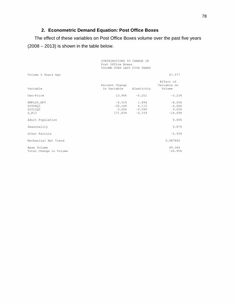
78

2. Econometric Demand Equation: Post Office Boxes The effect of these variables on Post Office Boxes volume over the past five years

(2008 – 2013) is shown in the table below.

CONTRIBUTIONS TO CHANGE IN Post Office Boxes VOLUME OVER LAST FIVE YEARS Volume 5 Years Ago 67.577 Effect of Percent Change Variable on Variable In Variable Elasticity Volume Own-Price 13.96% -0.251 -3.23% EMPLOY_HPT -4.31% 1.894 -8.00% D2008Q1 -30.16% 0.115 -4.06% D2012Q2 0.00% -0.099 0.00% D_R12 171.83% -0.159 -14.69% Adult Population 5.65% Seasonality 0.87% Other Factors -5.93% Mechanical Net Trend 0.987845 Base Volume 49.364 Total Change in Volume -26.95%

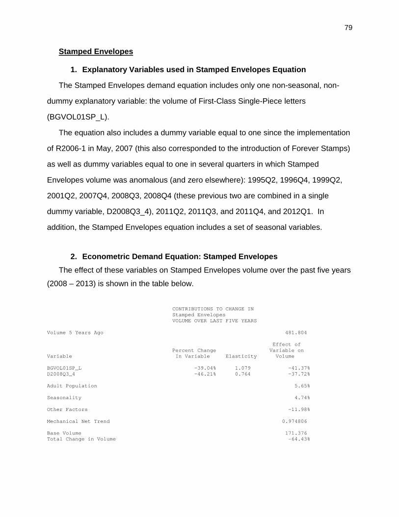
79

Stamped Envelopes

1. Explanatory Variables used in Stamped Envelopes Equation

The Stamped Envelopes demand equation includes only one non-seasonal, non-

dummy explanatory variable: the volume of First-Class Single-Piece letters

(BGVOL01SP_L).

The equation also includes a dummy variable equal to one since the implementation

of R2006-1 in May, 2007 (this also corresponded to the introduction of Forever Stamps)

as well as dummy variables equal to one in several quarters in which Stamped

Envelopes volume was anomalous (and zero elsewhere): 1995Q2, 1996Q4, 1999Q2,

2001Q2, 2007Q4, 2008Q3, 2008Q4 (these previous two are combined in a single

dummy variable, D2008Q3_4), 2011Q2, 2011Q3, and 2011Q4, and 2012Q1. In

addition, the Stamped Envelopes equation includes a set of seasonal variables.

2. Econometric Demand Equation: Stamped Envelopes

The effect of these variables on Stamped Envelopes volume over the past five years

(2008 – 2013) is shown in the table below.

CONTRIBUTIONS TO CHANGE IN Stamped Envelopes VOLUME OVER LAST FIVE YEARS Volume 5 Years Ago 481.804 Effect of Percent Change Variable on Variable In Variable Elasticity Volume BGVOL01SP_L -39.04% 1.079 -41.37% D2008Q3_4 -46.21% 0.764 -37.72% Adult Population 5.65% Seasonality 4.74% Other Factors -11.98% Mechanical Net Trend 0.974806 Base Volume 171.376 Total Change in Volume -64.43%

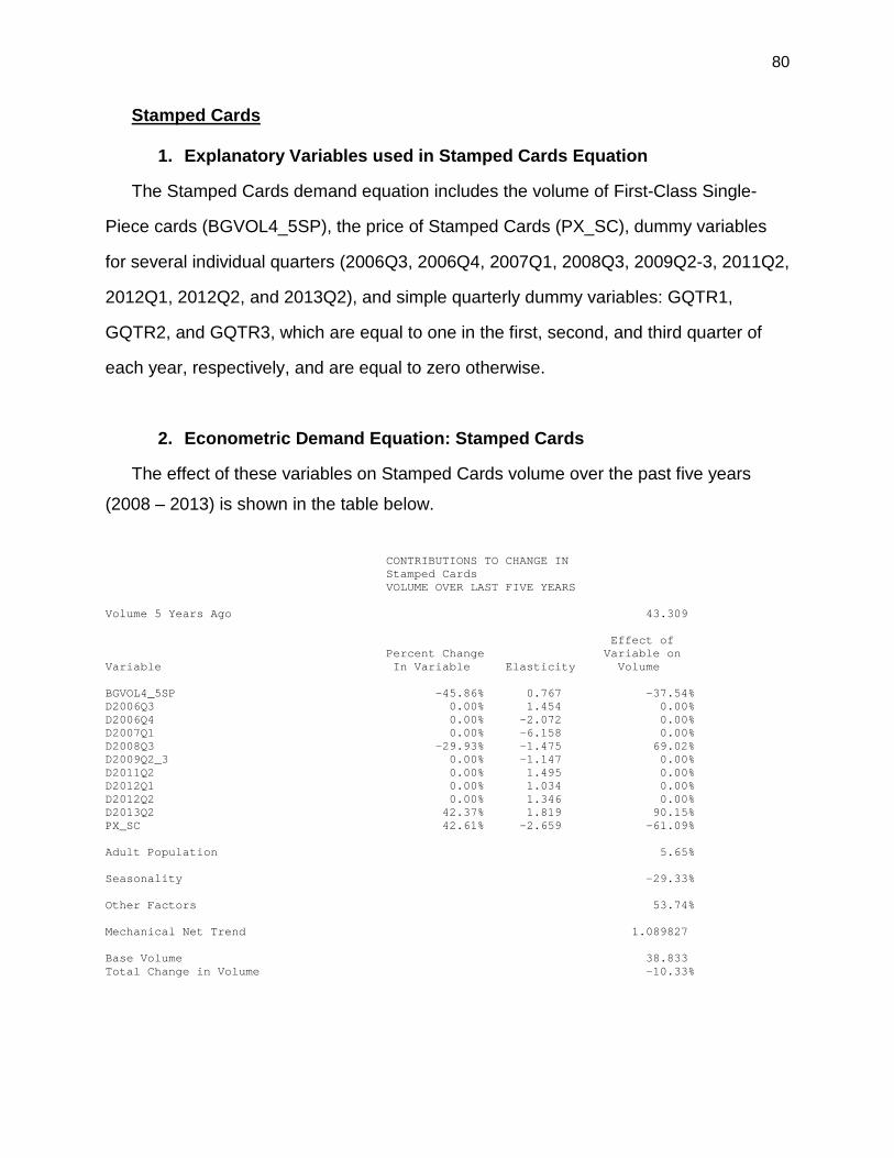
80

Stamped Cards

1. Explanatory Variables used in Stamped Cards Equation

The Stamped Cards demand equation includes the volume of First-Class Single-

Piece cards (BGVOL4_5SP), the price of Stamped Cards (PX_SC), dummy variables

for several individual quarters (2006Q3, 2006Q4, 2007Q1, 2008Q3, 2009Q2-3, 2011Q2,

2012Q1, 2012Q2, and 2013Q2), and simple quarterly dummy variables: GQTR1,

GQTR2, and GQTR3, which are equal to one in the first, second, and third quarter of

each year, respectively, and are equal to zero otherwise.

2. Econometric Demand Equation: Stamped Cards

The effect of these variables on Stamped Cards volume over the past five years

(2008 – 2013) is shown in the table below.

CONTRIBUTIONS TO CHANGE IN Stamped Cards VOLUME OVER LAST FIVE YEARS Volume 5 Years Ago 43.309 Effect of Percent Change Variable on Variable In Variable Elasticity Volume BGVOL4_5SP -45.86% 0.767 -37.54% D2006Q3 0.00% 1.454 0.00% D2006Q4 0.00% -2.072 0.00% D2007Q1 0.00% -6.158 0.00% D2008Q3 -29.93% -1.475 69.02% D2009Q2_3 0.00% -1.147 0.00% D2011Q2 0.00% 1.495 0.00% D2012Q1 0.00% 1.034 0.00% D2012Q2 0.00% 1.346 0.00% D2013Q2 42.37% 1.819 90.15% PX_SC 42.61% -2.659 -61.09% Adult Population 5.65% Seasonality -29.33% Other Factors 53.74% Mechanical Net Trend 1.089827 Base Volume 38.833 Total Change in Volume -10.33%

81

Delivery and Signature Confirmation

1. Dependent Variables used in Delivery and Signature Confirmation Equations

Delivery and Signature Confirmation volumes are divided into 14 distinct categories

which distinguish Delivery Confirmation from Signature Confirmation, retail confirmation

from electronic confirmation, and which distinguishes by the class of the parent piece of

mail being confirmed. This produces the following 14 distinct products:

Delivery Confirmation Retail First-Class Priority Package Services Electronic First-Class Priority Standard Parcel Select Package Services Signature Confirmation Retail First-Class Priority Package Services Electronic First-Class Priority Package Services

A separate demand equation is then estimated for each of these 14 products. The

dependent variables in these equations are set equal to the percentage of total volume

to which the relevant Confirmation service is attached, e.g., the dependent variable in

the First-Class Retail Delivery Confirmation demand equation is First-Class Retail

Delivery Confirmation volume divided by the total volume of First-Class parcels.

82

2. Explanatory Variables Used in Delivery and Signature Confirmation Equations

The Delivery and Signature Confirmation demand equations generally include the

following explanatory variables.

(1) Time Trend

Delivery and Signature Confirmation volume in its earliest years was characterized

by dramatic volume increases which decreased in intensity over time. To capture this,

the Delivery and Signature Confirmation demand equations typically include a logistic

time trend (T_DC).

(2) Postal Prices

Price indices measuring the average price of Delivery and Signature Confirmation

are included in the Delivery and Signature Confirmation demand equations for products

which have non-zero prices.

(3) Other Variables

Some of the Delivery and Signature Confirmation equations contain one or more

dummy variables reflecting either anomalous individual quarters or level shifts, typically

tied to rate changes. All of the Delivery and Signature Confirmation demand equations

also include simple quarterly dummy variables.

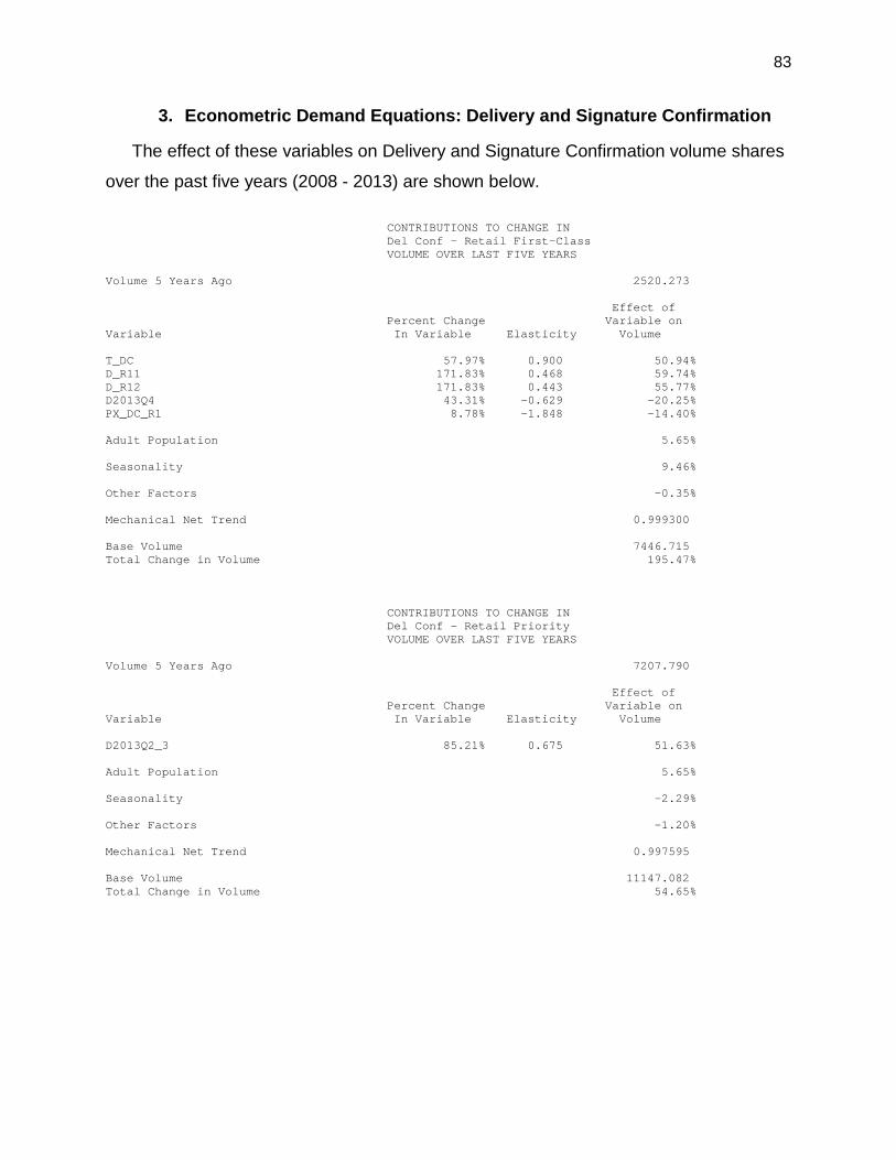
83

3. Econometric Demand Equations: Delivery and Signature Confirmation

The effect of these variables on Delivery and Signature Confirmation volume shares

over the past five years (2008 - 2013) are shown below.

CONTRIBUTIONS TO CHANGE IN Del Conf - Retail First-Class VOLUME OVER LAST FIVE YEARS Volume 5 Years Ago 2520.273 Effect of Percent Change Variable on Variable In Variable Elasticity Volume T_DC 57.97% 0.900 50.94% D_R11 171.83% 0.468 59.74% D_R12 171.83% 0.443 55.77% D2013Q4 43.31% -0.629 -20.25% PX_DC_R1 8.78% -1.848 -14.40% Adult Population 5.65% Seasonality 9.46% Other Factors -0.35% Mechanical Net Trend 0.999300 Base Volume 7446.715 Total Change in Volume 195.47% CONTRIBUTIONS TO CHANGE IN Del Conf - Retail Priority VOLUME OVER LAST FIVE YEARS Volume 5 Years Ago 7207.790 Effect of Percent Change Variable on Variable In Variable Elasticity Volume D2013Q2_3 85.21% 0.675 51.63% Adult Population 5.65% Seasonality -2.29% Other Factors -1.20% Mechanical Net Trend 0.997595 Base Volume 11147.082 Total Change in Volume 54.65%

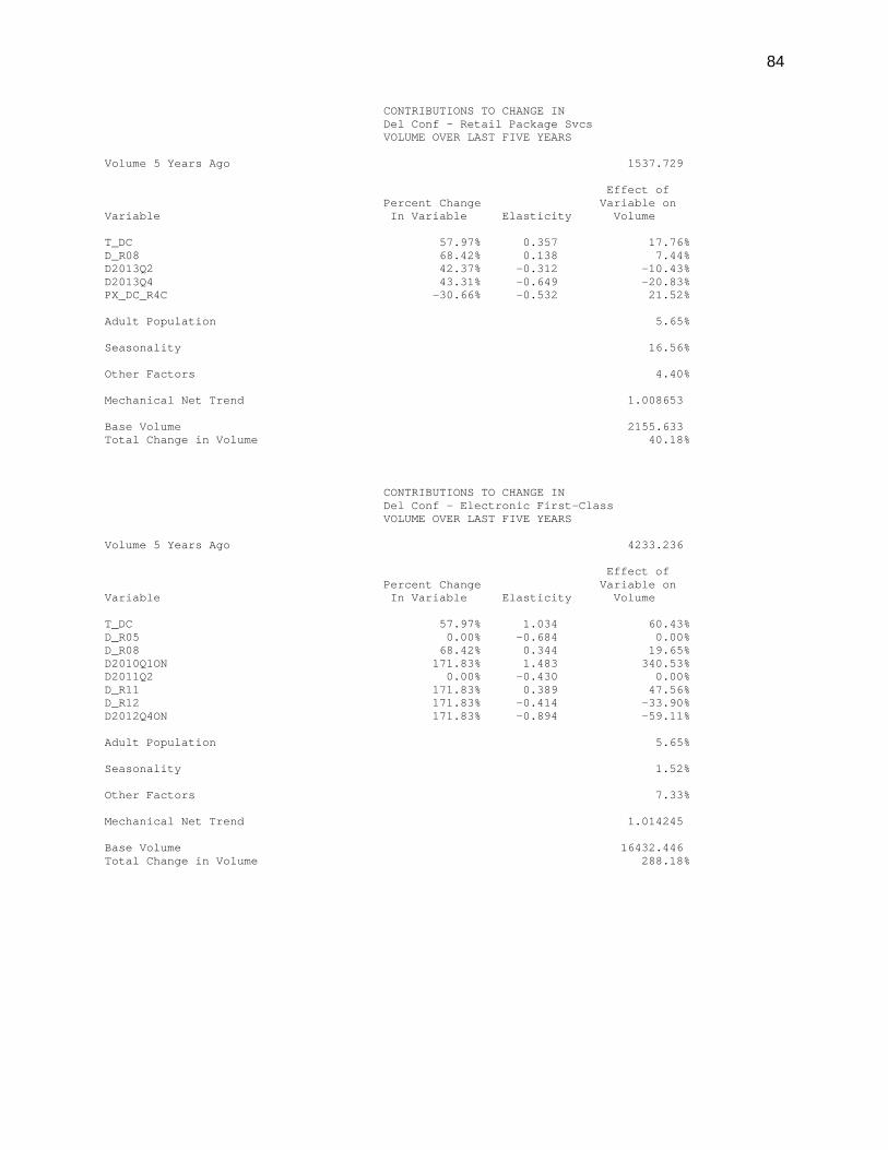
84

CONTRIBUTIONS TO CHANGE IN Del Conf - Retail Package Svcs VOLUME OVER LAST FIVE YEARS Volume 5 Years Ago 1537.729 Effect of Percent Change Variable on Variable In Variable Elasticity Volume T_DC 57.97% 0.357 17.76% D_R08 68.42% 0.138 7.44% D2013Q2 42.37% -0.312 -10.43% D2013Q4 43.31% -0.649 -20.83% PX_DC_R4C -30.66% -0.532 21.52% Adult Population 5.65% Seasonality 16.56% Other Factors 4.40% Mechanical Net Trend 1.008653 Base Volume 2155.633 Total Change in Volume 40.18% CONTRIBUTIONS TO CHANGE IN Del Conf - Electronic First-Class VOLUME OVER LAST FIVE YEARS Volume 5 Years Ago 4233.236 Effect of Percent Change Variable on Variable In Variable Elasticity Volume T_DC 57.97% 1.034 60.43% D_R05 0.00% -0.684 0.00% D_R08 68.42% 0.344 19.65% D2010Q1ON 171.83% 1.483 340.53% D2011Q2 0.00% -0.430 0.00% D_R11 171.83% 0.389 47.56% D_R12 171.83% -0.414 -33.90% D2012Q4ON 171.83% -0.894 -59.11% Adult Population 5.65% Seasonality 1.52% Other Factors 7.33% Mechanical Net Trend 1.014245 Base Volume 16432.446 Total Change in Volume 288.18%

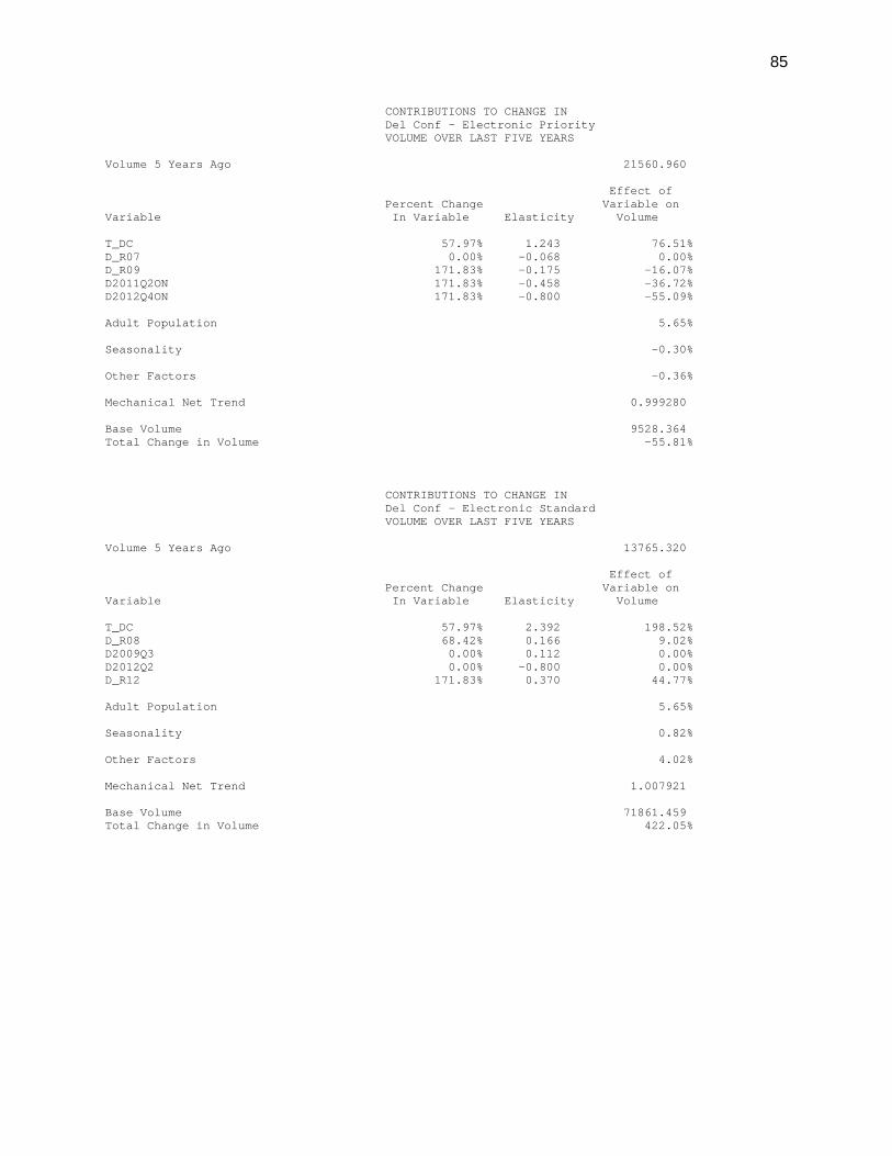
85

CONTRIBUTIONS TO CHANGE IN Del Conf - Electronic Priority VOLUME OVER LAST FIVE YEARS Volume 5 Years Ago 21560.960 Effect of Percent Change Variable on Variable In Variable Elasticity Volume T_DC 57.97% 1.243 76.51% D_R07 0.00% -0.068 0.00% D_R09 171.83% -0.175 -16.07% D2011Q2ON 171.83% -0.458 -36.72% D2012Q4ON 171.83% -0.800 -55.09% Adult Population 5.65% Seasonality -0.30% Other Factors -0.36% Mechanical Net Trend 0.999280 Base Volume 9528.364 Total Change in Volume -55.81% CONTRIBUTIONS TO CHANGE IN Del Conf - Electronic Standard VOLUME OVER LAST FIVE YEARS Volume 5 Years Ago 13765.320 Effect of Percent Change Variable on Variable In Variable Elasticity Volume T_DC 57.97% 2.392 198.52% D_R08 68.42% 0.166 9.02% D2009Q3 0.00% 0.112 0.00% D2012Q2 0.00% -0.800 0.00% D_R12 171.83% 0.370 44.77% Adult Population 5.65% Seasonality 0.82% Other Factors 4.02% Mechanical Net Trend 1.007921 Base Volume 71861.459 Total Change in Volume 422.05%

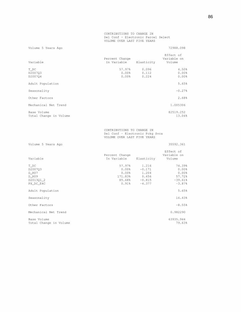
86

CONTRIBUTIONS TO CHANGE IN Del Conf - Electronic Parcel Select VOLUME OVER LAST FIVE YEARS Volume 5 Years Ago 72988.098 Effect of Percent Change Variable on Variable In Variable Elasticity Volume T_DC 57.97% 0.096 4.50% D2007Q3 0.00% 0.112 0.00% D2007Q4 0.00% 0.224 0.00% Adult Population 5.65% Seasonality -0.27% Other Factors 2.68% Mechanical Net Trend 1.005306 Base Volume 82519.252 Total Change in Volume 13.06% CONTRIBUTIONS TO CHANGE IN Del Conf - Electronic Pckg Svcs VOLUME OVER LAST FIVE YEARS Volume 5 Years Ago 35592.361 Effect of Percent Change Variable on Variable In Variable Elasticity Volume T_DC 57.97% 1.216 74.39% D2007Q3 0.00% -0.171 0.00% D_R07 0.00% 1.204 0.00% D_R09 171.83% 0.456 57.72% D2013Q1_2 85.68% -0.815 -39.61% PX_DC_E4C 0.91% -4.377 -3.87% Adult Population 5.65% Seasonality 16.43% Other Factors -8.55% Mechanical Net Trend 0.982290 Base Volume 63935.944 Total Change in Volume 79.63%

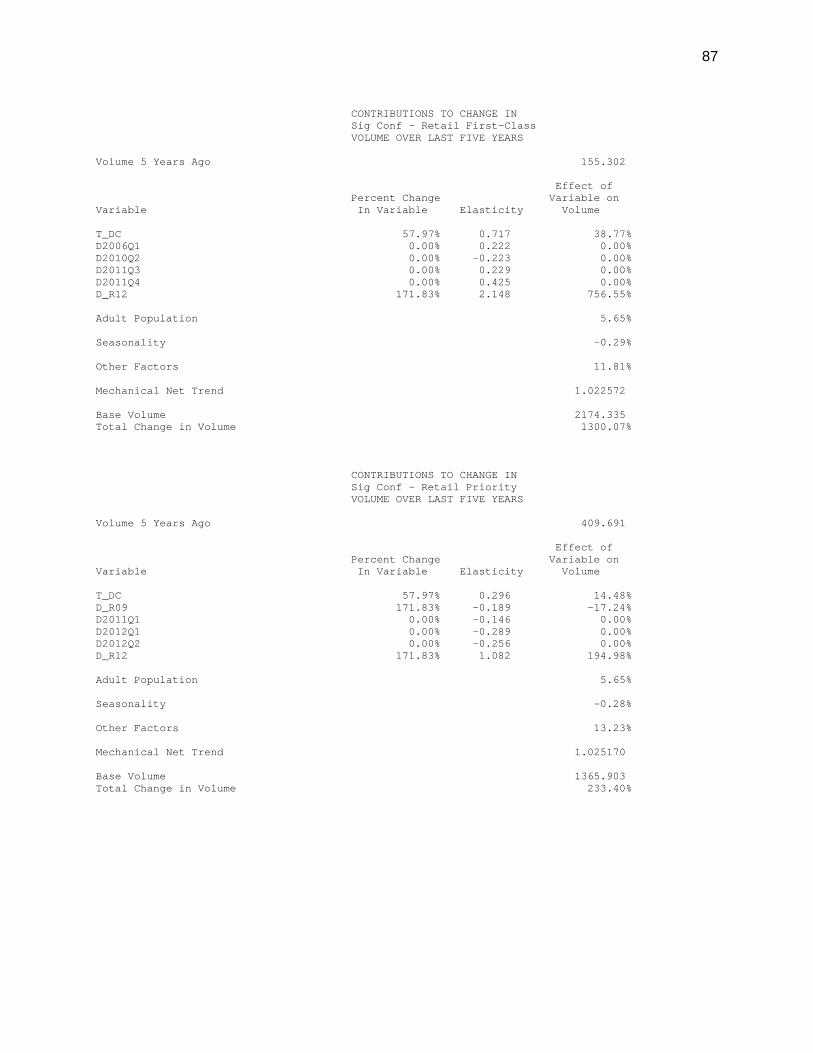
87

CONTRIBUTIONS TO CHANGE IN Sig Conf - Retail First-Class VOLUME OVER LAST FIVE YEARS Volume 5 Years Ago 155.302 Effect of Percent Change Variable on Variable In Variable Elasticity Volume T_DC 57.97% 0.717 38.77% D2006Q1 0.00% 0.222 0.00% D2010Q2 0.00% -0.223 0.00% D2011Q3 0.00% 0.229 0.00% D2011Q4 0.00% 0.425 0.00% D_R12 171.83% 2.148 756.55% Adult Population 5.65% Seasonality -0.29% Other Factors 11.81% Mechanical Net Trend 1.022572 Base Volume 2174.335 Total Change in Volume 1300.07% CONTRIBUTIONS TO CHANGE IN Sig Conf - Retail Priority VOLUME OVER LAST FIVE YEARS Volume 5 Years Ago 409.691 Effect of Percent Change Variable on Variable In Variable Elasticity Volume T_DC 57.97% 0.296 14.48% D_R09 171.83% -0.189 -17.24% D2011Q1 0.00% -0.146 0.00% D2012Q1 0.00% -0.289 0.00% D2012Q2 0.00% -0.256 0.00% D_R12 171.83% 1.082 194.98% Adult Population 5.65% Seasonality -0.28% Other Factors 13.23% Mechanical Net Trend 1.025170 Base Volume 1365.903 Total Change in Volume 233.40%

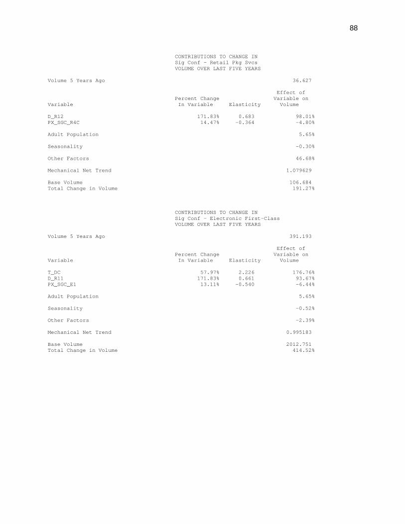
88

CONTRIBUTIONS TO CHANGE IN Sig Conf - Retail Pkg Svcs VOLUME OVER LAST FIVE YEARS Volume 5 Years Ago 36.627 Effect of Percent Change Variable on Variable In Variable Elasticity Volume D_R12 171.83% 0.683 98.01% PX_SGC_R4C 14.47% -0.364 -4.80% Adult Population 5.65% Seasonality -0.30% Other Factors 46.68% Mechanical Net Trend 1.079629 Base Volume 106.684 Total Change in Volume 191.27% CONTRIBUTIONS TO CHANGE IN Sig Conf - Electronic First-Class VOLUME OVER LAST FIVE YEARS Volume 5 Years Ago 391.193 Effect of Percent Change Variable on Variable In Variable Elasticity Volume T_DC 57.97% 2.226 176.76% D_R11 171.83% 0.661 93.67% PX_SGC_E1 13.11% -0.540 -6.44% Adult Population 5.65% Seasonality -0.52% Other Factors -2.39% Mechanical Net Trend 0.995183 Base Volume 2012.751 Total Change in Volume 414.52%

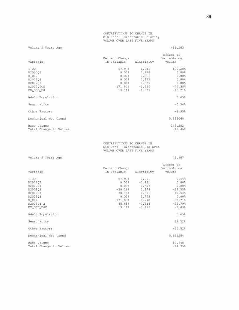
89

CONTRIBUTIONS TO CHANGE IN Sig Conf - Electronic Priority VOLUME OVER LAST FIVE YEARS Volume 5 Years Ago 493.203 Effect of Percent Change Variable on Variable In Variable Elasticity Volume T_DC 57.97% 1.615 109.28% D2007Q3 0.00% 0.178 0.00% D_R07 0.00% 0.366 0.00% D2012Q1 0.00% 0.329 0.00% D2012Q3 0.00% -0.539 0.00% D2012Q4ON 171.83% -1.286 -72.35% PX_SGC_E8 13.11% -1.339 -15.21% Adult Population 5.65% Seasonality -0.54% Other Factors -1.95% Mechanical Net Trend 0.996068 Base Volume 249.282 Total Change in Volume -49.46% CONTRIBUTIONS TO CHANGE IN Sig Conf - Electronic Pkg Svcs VOLUME OVER LAST FIVE YEARS Volume 5 Years Ago 49.307 Effect of Percent Change Variable on Variable In Variable Elasticity Volume T_DC 57.97% 0.201 9.64% D2006Q3 0.00% -0.481 0.00% D2007Q1 0.00% -0.507 0.00% D2008Q1 -30.16% 0.373 -12.53% D2008Q4 -30.16% 0.606 -19.54% D2012Q1 0.00% 0.773 0.00% D_R12 171.83% -0.770 -53.71% D2013Q1_2 85.68% -0.418 -22.79% PX_SGC_E4C 13.11% -0.199 -2.43% Adult Population 5.65% Seasonality 19.52% Other Factors -24.52% Mechanical Net Trend 0.945284 Base Volume 12.648 Total Change in Volume -74.35%