NASA TECHNICAL NOTE 7

A DIGITAL HIGHER ORDER INTERPOLATION PATH CONTROLLER

by WilZiam Granville Batte Langley Research Center Langley Station, Hampton, Va.

N A T I O N A L AERONAUTICS AND SPACE A D M I N I S T R A T I O N W A S H I N G T O N , D. C.

https://ntrs.nasa.gov/search.jsp?R=19660025916 2018-05-23T15:22:05+00:00Z

TECH LIBRARY KAFB, NM

NASA 'I" U-SD' i ' i

A DIGITAL HIGHER ORDER INTERPOLATION

PATHCONTROLLER

By William Granville Batte

Langley Research Center Langley Station, Hampton, Va.

N A T I O N A L AERONAUTICS AND SPACE ADMINISTRATION

For sale by the Clearinghouse for Federal Scientific and Technical Information Springfield, Virginia 22151 - Price $2.50

CONTENTS

SUMMARY . . . . . . . . . . . . . . . . . . . . . . . . . . . . . . . . . . . . . . . . 1

INTRODUCTION . . . . . . . . . . . . . . . . . . . . . . . . . . . . . . . . . . . . . 1

SYMBOLS AND NOTATIONS . . . . . . . . . . . . . . . . . . . . . . . . . . . . . . 4

GENERAL THEORETICAL CONSIDERATIONS . . . . . . . . . . . . . . . . . . . . . 8 Computational Algorithms . . . . . . . . . . . . . . . . . . . . . . . . . . . . . . 9 Derivation of Output Function . . . . . . . . . . . . . . . . . . . . . . . . . . . . . 11 Merging Function Criterion . . . . . . . . . . . . . . . . . . . . . . . . . . . . . . 18 Computationof p . . . . . . . . . . . . . . . . . . . . . . . . . . . . . . . . . . . 19

Principal Range of Angles . . . . . . . . . . . . . . . . . . . . . . . . . . . . . . 20 Equivalence of Angles . . . . . . . . . . . . . . . . . . . . . . . . . . . . . . . . . 20

COMPUTATIONOF + . . . . . . . . . . . . . . . . . . . . . . . . . . . . . . . . . 22

OPERATIONS OF THE EXPERIMENTAL MODEL . . . . . . . . . . . . . . . . . . . 28 28 31 33

+-computer subroutine . . . . . . . . . . . . . . . . . . . . . . . . . . . . . . . 34 Main program . . . . . . . . . . . . . . . . . . . . . . . . . . . . . . . . . . . . 37 Input progra& . . . . . . . . . . . . . . . . . . . . . . . . . . . . . . . . . . . . 45

DESIGN OF THE EXPERIMENTAL MODEL . . . . . . . . . . . . . . . . . . . . . . 47 50

Typical accumulator . . . . . . . . . . . . . . . . . . . . . . . . . . . . . . . . 50 Accumulator 3 . . . . . . . . . . . . . . . . . . . . . . . . . . . . . . . . . . . . 52 Accumulator 2 . . . . . . . . . . . . . . . . . . . . . . . . . . . . . . . . . . . . 52 Accumulator 4 . . . . . . . . . . . . . . . . . . . . . . . . . . . . . . . . . . . . 53 Shift pulse generator . . . . . . . . . . . . . . . . . . . . . . . . . . . . . . . . 53 Counter1 . . . . . . . . . . . . . . . . . . . . . . . . . . . . . . . . . . . . . . 56 Controls . . . . . . . . . . . . . . . . . . . . . . . . . . . . . . . . . . . . . . . 57 Binary rate multiplier . . . . . . . . . . . . . . . . . . . . . . . . . . . . . . . . 58 Counters 2 ,3 , and 4 . . . . . . . . . . . . . . . . . . . . . . . . . . . . . . . . 60

Theta Resolver . . . . . . . . . . . . . . . . . . . . . . . . . . . . . . . . . . . . 62 Merging Function . . . . . . . . . . . . . . . . . . . . . . . . . . . . . . . . . . . 62 Input . . . . . . . . . . . . . . . . . . . . . . . . . . . . . . . . . . . . . . . . . . 64

Registers . . . . . . . . . . . . . . . . . . . . . . . . . . . . . . . . . . . . . . . . 64 Accumulator 1 . . . . . . . . . . . . . . . . . . . . . . . . . . . . . . . . . . . . 64

General Description of Model . . . . . . . . . . . . . . . . . . . . . . . . . . . . . Simplified Operations of Model . . . . . . . . . . . . . . . . . . . . . . . . . . . . Detailed Operations of Model . . . . . . . . . . . . . . . . . . . . . . . . . . . . .

Design of the +.Computer . . . . . . . . . . . . . . . . . . . . . . . . . . . . . . . .

iii

DataEntry . . . . . . . . . . . . . . . . . . . . . . . . . . . . . . . . . . . . . . . 64 Code detector . . . . . . . . . . . . . . . . . . . . . . . . . . . . . . . . . . . . 64 BCD to binary converter . . . . . . . . . . . . . . . . . . . . . . . . . . . . . . 65 Two' s complementer . . . . . . . . . . . . . . . . . . . . . . . . . . . . . . . . 67

EXPElUMENTAL RESULTS . . . . . . . . . . . . . . . . . . . . . . . . . . . . . . . 68 Evaluation of Generated Curves . . . . . . . . . . . . . . . . . . . . . . . . . . . 68 . rc/' Boundaries . . . . . . . . . . . . . . . . . . . . . . . . . . . . . . . . . . . . 72 *-Computer Error . . . . . . . . . . . . . . . . . . . . . . . . . . . . . . . . . . 73 Initialization of (C3) . . . . . . . . . . . . . . . . . . . . . . . . . . . . . . . . . 73

RESEARCH BYPRODUCTS . . . . . . . . . . . . . . . . . . . . . . . . . . . . . . . 74

NEED FOR ADDITIONAL RESEARCH . . . . . . . . . . . . . . . . . . . . . . . . . 74

CONCLUDING REMARKS . . . . . . . . . . . . . . . . . . . . . . . . . . . . . . . . 75

APPENDIX - DERIVATION OF STEERING ANGLE Cp . . . . . . . . . . . . . . . . 77

REFERENCES . . . . . . . . . . . . . . . . . . . . . . . . . . . . . . . . . . . . . . 85

iv

A DIGITAL HIGHER ORDER INTERPOLATION

PATHCONTROLLER*

By William Granville Batte Langley Research Center

SUMMARY

A two-axis digital higher order interpolation path controller for generating a smooth incremental path through discrete Cartesian input data is designed, constructed, and evaluated.

The novel interpolation technique exhibits the following features:

(1) Its digital implementation is simple relative to classical higher order interpo- lation schemes.

(2) It is readily adaptable to incremental techniques and to the calculus of finite differences .

(3) It accommodates unequal argument spacing.

(4) It processes multivalued and closed contour functions.

(5) It can accommodate raw or nonpreprocessed data.

(6) It is readily expandable to multidimensions.

Although the controller may be applied in many areas including control of machine tools, navigation, simulation, function generation, remote control, and automatic plotting, the experimental model is evaluated with a standard incremental x-y plotter as the out- put device and a punched paper tape reader as the input device.

Laboratory tests were made on the implemented system and actual copies of its output are included. These results show that the approach is feasible and that the research objectives a r e met.

INTRODUCTION

The subject controller is a two-axis digital higher order interpolation device which generates a smooth incremental path through discrete, plane Cartesian input data. These data, which may fall into any one or more of the four quadrants, are sequentially ordered

The information presented herein was included in a thesis submitted in partial * fulfillment of the requirements for the degree of Doctor of Philosophy, Case Institute of Technology, Cleveland, Ohio, 1965.

as received so that the generated path follows this ordering. Since no attempt is made to f i t the data to some analytic function, the controller may be viewed as a device for auto- matically "applying the draftman's french curve. *'

Although the controller is developed for use in automatic plotting, it may be applied in many other areas including control of machine tools, navigation, simulation, function generation, and remote control. Also, the mathematical scheme may be used as an inter- polation technique for certain types of general purpose computing.

The controller is the result of research directed toward satisfying a need in auto- matic digital plotting. Automatic x-y plotters have replaced manual methods in most facilities where large quantities of data a r e displayed graphically. Most of these plotters produce point plots in which a pen or symbol head marks the locations corresponding to the various discrete x-y input values. In addition, some plotters (e.g., the Beckman 210 tape-to-plotter system) can also produce continuous curves in which the discrete input data a r e connected by straight-line segments. Not one plotter, however, is effective in "placing the french curve through the points" as was commonly done in the manual methods. controller capable of supplying the "french curve" even under conditions of (a) data with unequal argument spacing, (b) mul-tivalued or closed contour functions, and (c) raw or nonpreprocessed data. Secondary objectives require the hardware to be relatively simple and fast enough to keep the output device operating at its inherent maximum speed.

Consequently the primary objective of this research is to evolve a simple

Numerous digital controllers a r e in existence but each fails in one or more ways to satisfy these objectives. For example, Mergler's machine tool controller (ref. 1) requires rate information to be supplied as a part of the input data and, hence, does not satisfy condition (c). His proposed quadratic (second order) technique recognizes its inadequacies for certain "geometry" and, in addition, requires "equal intervals of the argument,'' each of which renders the scheme inadequate for the present application.

Several second-order systems a r e in existence but they too do not satisfy condi- tion (c). For example, the Bendix Dynapath system (ref. 2) requires, for circular inter- polation, that the initial and final positions of the radius vectors be supplied as a portion of the input data. Similarly, the Fuji system (ref. 3) requires that the input data be expressed in a coordinate system whose origin is at the center of the arc. Even more serious, however, is that the present application requires at least a third-order interpo- lation as demonstrated in reference 4.

Ninke (ref. 5) recently adapted the Newton-Gauss interpolation technique to a digital third-order controller. Using digital differential analyzer (DDA) methods, the system consists of three digital integrators cascaded so that the third derivative introduced at the first integrator is successively integrated three times, this integration yielding the path function at the output of the last integrator. The initial conditions of the integrators

2

and corrections thereto must be supplied as a portion of the input data; hence, condi- tion (c) is violated. Also the simplicity with which these quantities are computed is a result of the assumption by Ninke that the input data are spaced at equal increments of the arguments; hence, condition (a) is also violated.

A similar scheme is outlined in reference 6 where again the approach is based on equal arguments.

A s with most digital systems the controller has its analog counterpart. In many situations, however, the accuracy requirement renders the analog approach ineffective. Consider, for example, even simple linear interpolation where it is required to connect two points with a straight line. This problem is approached with the conventional analog closed-loop plotter by integrating the inputs to the two axes with the same effective time constants. The solution sounds simple, but the word "effective" requires a considera- tion of the unbalanced inertias and frictions on the two axes, the unbalanced breakaway torques, and, of course, settings of gain, damping, and so forth. Furthermore, higher- order interpolation is even more complex!

The study of existing controllers and classical interpolation techniques as applied to the performance requirements of the subject controller leads to the following broad observations which a re presented in the nature of hypotheses upon which the controller's design is based

(1) It is not important to f i t the input data to some analytic function (e.g., a third- degree polynomial or perhaps some french curve logarithmic function); instead, it is more important to utilize some hardware-oriented (though perhaps less mathematical) scheme such as a goal seeking system.

(2) Since the entire path must be generated, as opposed to merely evaluating a few isolated function values, a finite difference technique should be utilized such that the function change is computed and used to update the function along the generated path.

(3) Since the finite difference technique will no doubt result in many isolated arith- metic units, the internal coding should be natural binary with negative numbers repre- sented in two's complement notations. This coding will simplify the designs of the units.

(4) Since any closed contour path contains at least two infinite slopes, a technique which obviates the large slope problem (refs. 5 and 6) must be used.

(5) For simplicity of the experimental hardware, an incremental, open-loop control system should be used. (Where applications require absolute or incremental closed-loop systems, the experimental design is easily adapted to them.)

(6) Since the path must be generated from any data point through the next point, the direction of the latter point with respect to the present position of the generated path is an important variable and should probably appear explicitly in the basic interpolation scheme.

3

Other philosophies peculiar to various par ts of the controller are found in the appropriate design sections.

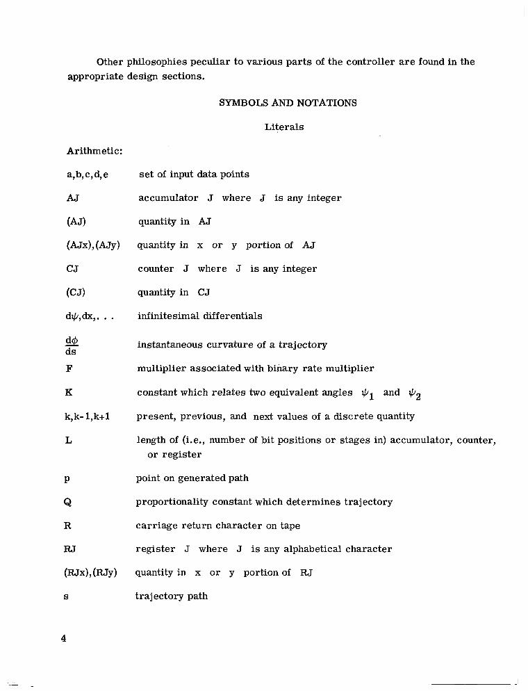
SYMBOLS AND NOTATIONS

Literals

Arithmetic:

a,b,c,d, e

AJ accumulator J where J is any integer

(AJ) quantity in AJ

(AJx),(AJy) quantity in x or y portion of AJ

CJ counter J where J is any integer

(c J) quantity in C J

dlC/,dx,. . . infinitesimal differentials

set of input data points

* ds

F

K

k,k- l,k+l

L

P

Q

R

RJ

S

instantaneous curvature of a trajectory

multiplier associated with binary rate multiplier

constant which relates two equivalent angles +hl and q2

present, previous, and next values of a discrete quantity

length of (Le., number of bit positions or stages in) accumulator, counter, or register

point on generated path

proportionality constant which determines trajectory

carriage return character on tape

register J where J is any alphabetical character

quantity in x or y portion of R J

trajectory path

4

sc 1

SWJ

6 (c4c)

6Q,6x,. . . A

AQ,A@,. ' *

E

e

4

P

4

Q

ICJ I

sign of quantity within brackets

switch J where J is any integer or alphabetical character

Cartesian coordinates

tangent angle of generated path at last data point

tangent angle of generated path at next data point

corrected e r ro r distance between grid corner and s-curve-grid-line inter section

change in coarse portion of quantity in counter 4

finite difference o r change in Q, x, . . .

"space" character on tape separating x- and y-data

total change in Q, @, . . .

e r ro r between @ and OC

motion angle required for coincidence with s-curve at next grid crossing; subscript c o r f denotes coarse o r fine portion of 8, respectively

merging function which starts from Qc and ends at @

predicted e r ro r distance between grid corner and s-curve-grid-line intersection

steering angle o r instantaneous angle of tangent to theoretical trajectory

angle of present position with respect to next data point

absolute value of (CJ)

Pr ime with symbol indicates quantity is expressed in transformed coordinate system.

5

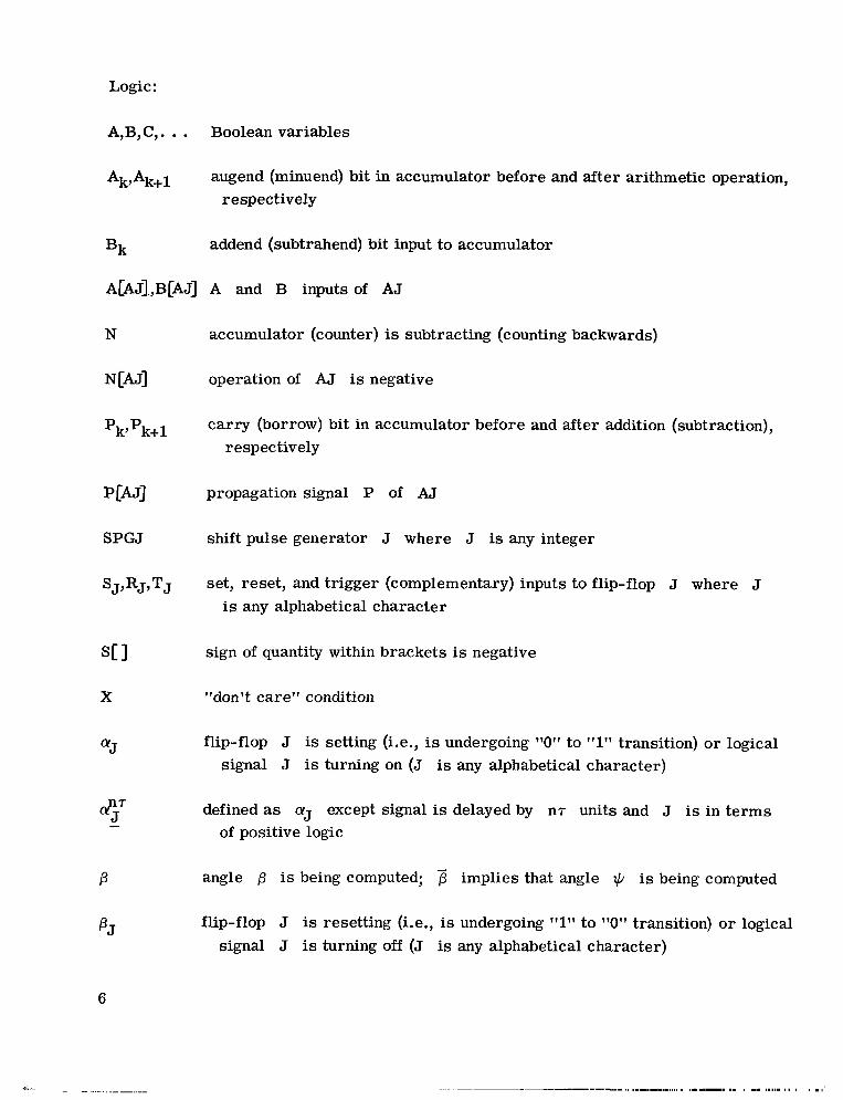
Logic:

A,B,C,. . .

Ak,Ak+l

Bk

ALA J]., B [A J]

Boolean variables

augend (minuend) bit in accumulator before and after arithmetic operation, respectively

addend (subtrahend) bit input to accumulator

A and B inputs of AJ

accumulator (counter) is subtracting (counting backwards)

operation of AJ is negative

carry (borrow) bit in accumulator before and after addition (subtraction), respectively

propagation signal P of AJ

shift pulse generator J where J is any integer

set, reset, and trigger (complementary) inputs to flip-flop J where J is any alphabetical character

sign of quantity within brackets is negative

"don't care" condition

flip-flop J is setting (Le., is undergoing "0" to "1" transition) or logical signal J is turning on (J is any alphabetical character)

defined as aJ except signal is delayed by n7 units and J is in terms of positive logic

angle p is being computed; 3 implies that angle Q is being computed

flip-flop J is resetting (i.e., is undergoing "1" to "0" transition) o r logical signal J is turning off (J is any alphabetical character)

~b .- ... .. . .. . . .__

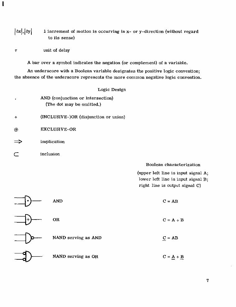
I6x1,16yl 1 increment of motion is occurring in x- or y-direction (without regard to its sense)

7 unit of delay

A bar over a symbol indicates the negation (or complement) of a variable.

An underscore with a Boolean variable designates the positive logic convention; the absence of the underscore represents the more common negative logic convention.

Logic Design

AND (conjunction or intersection) (The dot may be omitted.)

+

0

* C

(INCLUSIVE-)OR (disjunction or union)

EXCLUSIVE- OR

implication

inclusion

Boolean characterization

(upper left line is input signal A; lower left line is input signal B; right line is output signal C)

-D- AND

-b- OR

NAND serving as AND 3)- NAND serving as OR 3)-

C = A B

C = A + B

- C = A B

C = A + B - -

7

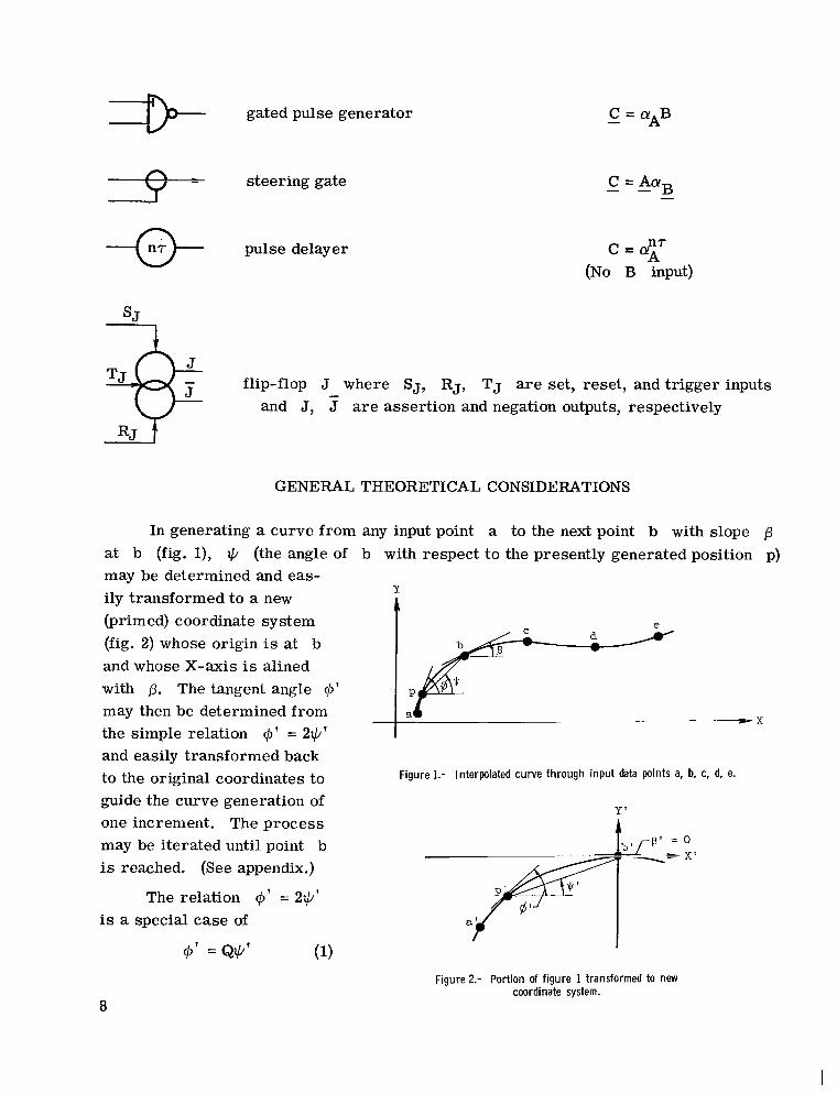
I

P

gated pulse generator

steering gate

pulse delayer

C = AaB - - -

C - C (No B input)

flip-flop J where SJ, RJ, TJ a r e set, reset, and trigger inputs and J, 5 are assertion and negation outputs, respectively

GENERAL THEORETICAL CONSIDERATIONS

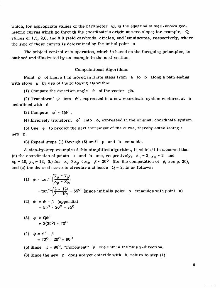
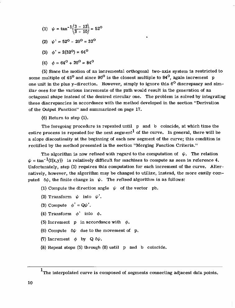
In generating a curve from any input point a to the next point b with slope p at b (fig. l), I) (the angle of may be determined and eas- ily transformed to a new (primed) coordinate system (fig. 2) whose origin is at b and whose X-axis is alined with p. The tangent angle 6' may then be determined from the simple relation @ ' = 21)' and easily transformed back to the original coordinates to guide the curve generation of one increment. The process may be iterated until point b is reached. (See appendix.)

The relation 6' = 2I)' is a special case of

@' =&I)' (1)

b with respect to the presently generated position p)

Y

Figure 1.- Interpolated curve through input _ . A points a, b, c, d, e.

Y' A

8

Figure 2.- Portion of f igure 1 transformed to new coordinate system.

which, for appropriate values of the parameter Q, is the equation of well-known geo- metric curves which go through the coordinate's origin at zero slope; for example, Q values of 1.5, 2.0, and 3.0 yield cardioids, circles, and lemniscates, respectively, where the size of these curves is determined by the initial point a.

The subject controller's operation, which is based on the foregoing principles, is outlined and illustrated by an example in the next section.

Computational Algorithms

Point p of figure 1 is moved in finite steps from a to b along a path ending with slope p by use of the following algorithm:

(1) Compute the direction angle I) of the vector pb.

(2) Transform I) into I)', expressed in a new coordinate system centered at b and alined with p.

(3) Compute @' = Qq' . (4) Inversely transform 4' into 4, expressed in the original coordinate system.

(5) Use @ to predict the next increment of the curve, thereby establishing a new p.

(6) Repeat steps (1) through (5) until p and b coincide.

A step-by-step example of this simplified algorithm, in which it is assumed that (a) the coordinates of points a and b are, respectively, X a = 3, Ya = 2 and Xb = 10, yb = 12, (b) for xa 5 xp < xb, p = 200 (for the computation of p, see p. 20), and (c) the desired curve is circular and hence Q = 2, is as follows:

= tan- ~ - l2 = 55O (since initially point p coincides with point a) (3 - 10) (2) I)' = I) - p (appendix)

= 550 - 200 = 350

(3) 4' = QI)' = 2(35O) = 70'

(4) 4 = 4' + P = 70' + 20° = 90'

(5) Since 4 = 90°, "increment" p one unit in the plus y-direction.

(6) Since the new p does not yet coincide with b, return to step (1).

9

1 3 - 1 2 (1) rc/ = tan- - (3 - 10) = 520 . (2) rc/' = 52O - 20' = 32'

(3) Cp' = 2(32O) = 64'

(4)

(5) Since the motion of an incremental orthogonal two-axis system is restricted to some multiple of 45' and since 90' is the closest multiple to 84O, again increment p one unit in the plus y-direction. However, simply to ignore this 6' discrepancy and sim- ilar ones for the various increments of the path would result in the generation of an octagonal shape instead of the desired circular one. The problem is solved by integrating these discrepancies in accordance with the method developed in the section "Derivation of the Output Function" and summarized on page 17.

Cp = 64' + 20' = 84'

(6) Return to step (1).

The foregoing procedure is repeated until p and b coincide, at which time the 1 entire process is repeated for the next segment of the curve. In general, there will be

a slope discontinuity at the beginning of each new segment of the curve; this condition is rectified by the method presented in the section "Merging Function Criteria."

The algorithm is now refined with regard to the computation of rc/. The relation rc/ = tan-l(f(x,y)) is relatively difficult for machines to compute as seen in reference 4. Unfortunately, step (1) requires this computation for each increment of the curve. Alter- natively, however, the algorithm may be changed to utilize, instead, the more easily com- puted 6rc/, the finite change in rc/. The refined algorithm is as follows:

(1) Compute the direction angle rc/ of the vector pb.

(2) Transform IC/ into @'.

(3) Compute @' = Qq'.

(4) Transform 4' into @.

(5) Increment p in accordance with @.

(6) Compute 61) due to the movement of p.

(7) Increment @ by Q 6@.

(8) Repeat steps (5) through (8) until p and b coincide.

The interpolated curve is composed of segments connecting adjacent data points, 1

10

This algorithm is advantageous in that the slow computations of steps (1) through (4) are performed once, with only the fast operations of steps (5) through (8) iterated for each increment of the curve.

Step (7) is based on the difference equation

@k+l = @k + Q 6+k

Since, by the fundamental difference definition

@k+l = @k + 6@k

it is necessary to show only that

6@k = Q 6+k

By the invariance property of the linear transformation (appendix),

6@k = 6@k By the fundamental definition,

6@k = @k+1 - @k

Again, by the fundamental definition,

6@k = Q W'k

Finally, by the invariance property,

6@k = Q Wc/k

Derivation of Output Function

Step (5) of the refined algorithm requires that p be incremented "in accordance with @." The coarse 45' angular resolution inherent in the output of an incremental, orthogonal, two-axis system poses a problem, in this instance, since such a system must generate @, a function of considerably finer resolution.

The problem is first approached in a precise manner. From this approach a com- plicated partial solution is obtained. Then applied is an approximation which yields a complete and greatly simplified solution without, for most applications, excessively degrading the results.

11

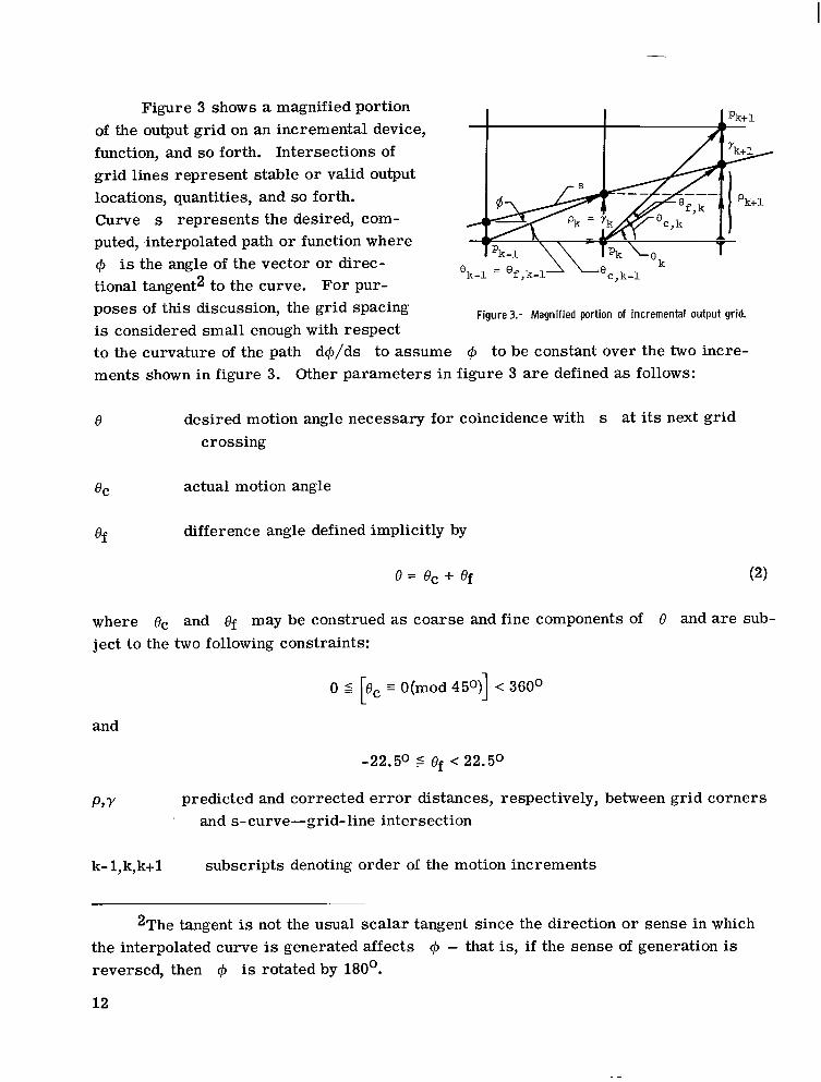
Figure 3 shows a magnified portion of the output grid on an incremental device, function, and so forth. Intersections of grid lines represent stable or valid output locations, quantities, and so forth. Curve s represents the desired, com- puted, interpolated path or function where @ is the angle of the vector or direc- tional tangent2 to the curve. For pur- poses of this discussion, the grid spacing is considered small enough with respect to the curvature of the path d@/ds to assume @ to be constant over the two incre- ments shown in figure 3.

Figure 3.- Magnified portion of incremental output grid.

Other parameters in figure 3 a r e defined as follows:

e desired motion angle necessary for coincidence with s at its next grid crossing

BC actual motion angle

difference angle defined implicitly by Of

e = ec + ef

where ec and Of may be construed as coarse and fine components of e and are sub- ject to the two following constraints:

and

-22.50 s ef < 22.50

P, Y predicted and corrected e r ro r distances, respectively, between grid corners and s-curve-grid-line intersection

k- l,k,k+l subscripts denoting order of the motion increments

2The tangent is not the usual scalar tangent since the direction or sense in which the interpolated curve is generated affects @ - that is, i f the sense of generation is reversed, then @ is rotated by 180'.

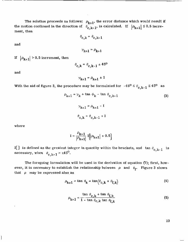
The solution proceeds as follows: pk+l, the e r ro r distance which would result if the motion continued in the direction of Oc,k- 1, is calculated. If I pk+l I = < 0 .5 incre- ment, then

'c,k = 'c,k- 1

and

rk+l = pk+l

If Ipk+ll > 0.5 increment, then

'c,k = 'c,k-l f 450

and

?/k+l = pk+l * With the aid of figure 3, the procedure may be formulated for -45' 5 'c,k-l 5 - 450 as

(3) pk+l = ?/k + tan @k - tan 'c,k-1

'c,k = 'c,k-l + I

where

I[] is defined as necessary, when

the greatest integer in quantity within the brackets, and tan Bc,k-l is Bc,k-1 = &5O.

The foregoing formulation will be used in the derivation of equation (7); first, how- ever, it is necessary to establish the relationship between p and Of. Figure 3 shows that p may be expressed also,as

13

For e take place when

= 0, equation (4) reduces to pk+l = tan e,,,. Hence, a change in e c,k c,k should

For e = +45O, equation (5) reduces to c,k

cos 2 ef k + 2 cos ef k sin ef k + sin 2 ef k - 9 9 7 9 -

2 f , k

cos e - sin20 f, k

1 + 2 cos Of k sin Of k 1 + sin 20f

f , k 9 - 7 - - -

2 COS 2e 1 - 2 sin 8 f , k

(6) f,k = sec 28 + t an28

pk+l f, k

Although the inverse ef, k(pk+l) is more complicated,. it is easily seen by substitu- tion that a change in 0 should occur when

c,k

> (45' - 26.6' = 18.4')

that is, when 0 < -18.4'. f , k

Finally, for e = -45O, equation (5) reduces to

-1 + tan Of k

f,k

c,k

= 1 + tan e '

Following the foregoing procedure results in

pk+l = tan 2ef,, - sec 28 f,k

and, hence, a change in 8 should occur when 8 > +18.4'.

Even considering only these limited cases, the pk+1 function is relatively com- c,k f , k

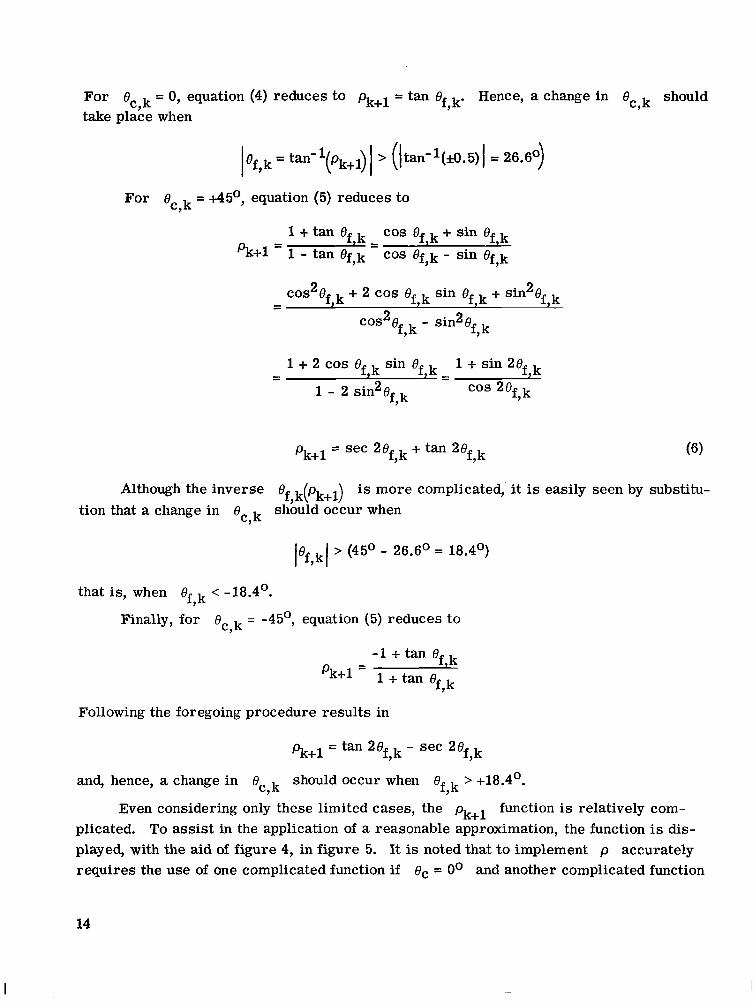
plicated. To assist in the application of a reasonable approximation, the function is dis- played, with the aid of figure 4, in figure 5. It is noted that to implement p accurately requires the use of one complicated function if OC = Oo and another complicated function

14

45.0

42.0

38.7

35.0

31.0

26.6

21.8

16.7

11.3

5.7

0.0

for -

a, = 45'

-0.0

-3.0

-6.3

-10.0

-14.0

-18.4

-23.2

-28.3

-33.7

-39.3

-45.0

- &f deg -

3 -0

3.3

3.7

4.0

4.4

4.8

5.1

3.4

5.6

5.7

Figure4.- Error angle Of for various error distances p.

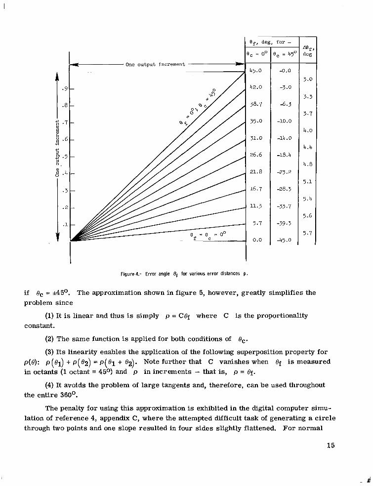
if problem since

eC = d 5 c . The approximation shown in figure 5, however, greatly simplifies the

(1) It is linear and thus is simply p = C8f where C is the proportionality constant .

(2) The same function is applied for both conditions of 8,.

(3) Its linearity enables the application of the following superposition property for p(8): p (el) + ~ ( 8 2 ) = p( 8 1 + 82). Note further that C vanishes when Of is measured in octants (1 octant = 450) and p in increments - that is, p = Of.

(4) It avoids the problem of large tangents and, therefore, can be used throughout the entire 360'.

The penalty for using this approximation is exhibited in the digital computer simu- lation of reference 4, appendix C, where the attempted difficult task of generating a circle through two points and one slope resulted in four sides slightly flattened. For normal

15

0 10 20 30 40 Error angle, Te,, deg

Figure 5.- Relation between actual and approximate error angle Of and error distance p .

curve interpolation tasks, however, this slight tendency to flatten is insignificant. implementation, therefore, is based on the use of this approximation.

The

In effect, then, the approximation establishes an equivalence relation between angular dimensions at pk of figure 3 and linear dimensions at the crossing, so that the tangent functions a r e eliminated and thereby the useful angular domains a r e extended throughout the entire 360°. Implicit in the relationship p = Of is the corrected form y = Of (where the constraints of equation (2) have been applied to the latter Of). Hence equation (3) can be written as

pk+l increment

'f,k = 'f,k-l + @k - 'c,k-l (7)

where the constraints of equation (2) are not yet applied to Of,k. By updating the subscripts

'f,k+l = 'f,k + @k - 'c,k (8 )

16

where, as assumed, @k+l = Cpk' Therefore,

Integrating finitely (ref. 7) gives

k- 1 P

'f,k = 'f,O + 2 6ef,j j=O

where j is a dummy variable. By letting the initial condition 0 = 0, f,O

k- 1

ef,k= 2 E j j=O

(9)

where E j = 68f,j = 4. - 8c,j, the e r ro r between the tangent angle of curve s and the actual motion angle. Hence equation (2) can be written

J

When 1 E j exceeds the constraints of equation (2), 1 or more octants are transferred

from 2 E j to BC. Equation (9) is a most important result since step (5) of the refined

algorithm can now be stated explicitly:

(1) Determine 8 for each point pk along the generated path by finitely inte- f,k

grating or summing the e r ro r ~j from initial = 0 to ~ k - ~ , continually applying the constraints associated with equation (2).

(2) Use equation (2) and associated constraints to establish e for each c,k

point pk'

(3) Generate the path in the direction of ec,k'

Thus, ~j as previously defined represents the e r ro r introduced at the jth step because the actual direction of travel 8,,j differs from the computed direction @j.

, the finite integral of this e r ro r integrated from an input data point po Whenever

to the previous generated point pk-l, exceeds 22- , it applies to a 4 5 O correction which, in general, is an overcorrection, in which case E j changes sign and 8 builds up in the opposite sense. Hence the actual path (controlled by 8,) continually seeks and, in general, follows the computed path (controlled by

lo 2 c,k

Pf,kI 8

f ,k

@) to within 0.5 increment. In

17

I

I I I I II 111 1111 111 I 1 1 1 1 1 I I I 1 1 1 1 1111 I I I I I, I, I I. .I. m ... I ...I - I.

I

t e rms of the CalComp digital incremental recorder model 565 that was used in this research, this 0.5 increment represents an e r r o r of 0.005 inch, a distance approximately as small as the plotted curve thickness.

The beauty of this formulation is that it is easily implemented.

Merging Function Criterion

In generating a curve from point a to point b, the refined algorithm of page 10 gives no consideration to the angle at which the curve originally entered a. In general, disregard of this angle results in derivative discontinuities at the various input data points of a curve.

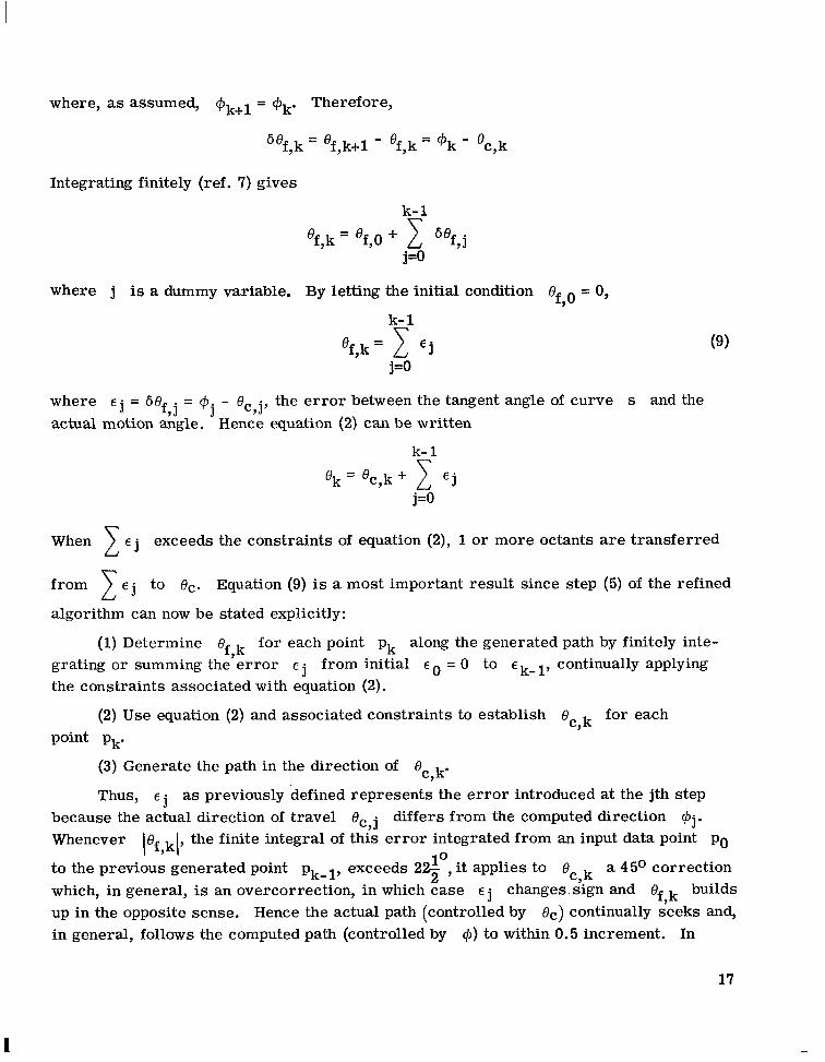
To obviate this problem, a merging function is derived which effects a smooth derivative transition from the curve entering some point to the curve leaving this point by limiting d@/ds, the curvature of the path in the vicinity of the point. The particular merging function criterion which is implemented may be considered to be circular since it limits d@/ds to the d@/ds of a circle whose diameter is equal to the distance between the present position p and the next data point. u re 6 d@/ds is constant over the path s; hence,

For the circle shown in fig-

(10) 2 radians 2 radians 3 - - 2nradians - - - 5 - ds n% increments % increment - dp increment

If d@/ds is limited to 2/% for an interpolated path, the merging function gives, in general, (1) a smooth transition, and (2) complete merging before p coincides with b.

Although other merging criteria could have

it is a simple function of dp, the square of which is already computed by the experimental hardware for other purposes.

been used, this particular one is attractive since b

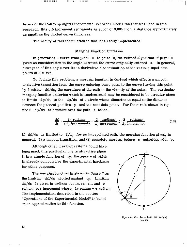
The merging function is shown in figure 7 as the limiting d@/ds plotted against dp. Limiting d@/ds is given in radians per increment and n radians per increment where ln radian = n radians. The implementation described in the section "Operations of the Experimental Model" is based on an approximation to this function.

Figure 6.- Circular criterion for merging function.

18

1. ooc

.50c

. loo

.050

. 010

.005

. 001 1 5 10 50 100

Distance to next point, dp, increments

Figure 7.- Merging function.

Computation of p

500 1000

The development of the theory is based on the hypothesis that the slope angle p of figure 1 is given. An examination of this hypothesis is now made.

In general, a unique accurate slope angle p does not exist since the input points do not specify the curve in the immediate neighborhood of point b - that is, in digital terms, the input points do not specify the increments immediately preceding and following point b. Therefore, the slope assigned to point b is a function of the particular

19

interpolation scheme used. On the assumptions that sufficient input points are given to faithfully represent the function and that point b lies in the middle 50-percent region

1 of the distance between a and c or, more precisely, - < h < 3, where h is the ratio of the distance ab to the distance ac , then the simple first difference definition of

( 3

is, in general, adequate as is seen by examining the geometry of various three-point patterns.

Equivalence of Angles

Physically I), @, p, and so forth, can range only over 2a radians. Hence, physical significance is extended to those values outside of range by letting the equiva- lence relation

qc/2

mean q1 = q2 + 2aK for some integer K (Le., ql = q2(mod 2 a)> . Principal Range of Angles

With the aid of the foregoing equivalence relation, IC/' in any range may be con- verted to its principal range defined as

-a 5 q' < +a

The important relation @ ' = w' tacitly assumes that q' is expressed in its principal range. However, it is shown in the following theorem that this requirement is really not a necessary condition when Q is an integer; that is, for the relation 4 ' = QG' equiv- alent angles @' are obtained for equivalent angles Q' when Q is an integer.

Theorem: Under the relations

$1 =

$2 = Qq2 q2 = ql(mod m) where m is any real number,

if Q is an integer then @2 @l(mod m).

Proof: (1) q2 ql(mod m), by hypothesis.

(2) q2 = + mK, by the equivalence definition.

(3) G2 = Qq2, by hypothesis.

20

(4) @2 = Q(Q1 + mK), bY steps (2) and (3)-

(5) G2 = @.l + mKQ, by hypothesis.

(6) Q is an integer, by hypothesis.

(7) KQ is an integer, since the product of two integers is an integer.

(8) Therefore @2 @l(mod m), by steps (5) and (7) and the equivalence definition.

The converse is not true. However, an important fact concerning the converse is stated in the following corollary to the theorem.

Corollary: Under the relations of the theorem, the equivalence of @1 and G2

This corollary is a consequence of step (7) of the theorem proof; that is, although specific cases can be found in which KQ is an integer for a noninteger value of Q, an integer product is assured only if both K and Q a r e integers.

is guaranteed only if Q is an integer.

These considerations - angular equivalence, principal range, and integer values Their signifi- of Q - a re extremely important in terms of hardware implementation.

cance will be briefly mentioned so that they can be more fully appreciated when the actual design of the experimental model is presented in a subsequent section.

The angle equivalence relation

q2 Ql(mod 27r)

implies that the hardware need not distinguish angles which differ by integral multiples of 27r. handle precisely the modulus 27r range and, hence, bit positions of weight P27r need not be provided even though the angle may exceed 27r.

Therefore the associated counters, registers, and so forth, a r e required to

The theorem essentially states that the complication associated with the principal range constraint can be avoided if one is satisfied with interpolated curves involving only integer values of Q - that is, Q = 1, the linear case, Q = 2, the circular case, and so forth. Utilizing only integer values of Q would greatly simplify the system control problem and could eliminate the binary rate multiplier in the design of the experimental model. The importance of noninteger Q in a practical operational device can best be established through operational experience. The more complicated noninteger Q capa- bility is therefore retained in the model design so that some measure of its importance may be acquired through use of the experimental device.

21

COMPUTATION OF + Perhaps the most important single

function to be performed in the interpo- lation scheme is the computation of

+ = tan- 1 9 Ax

or, if one of the points is at the origin as in figure 8,

Thus, with a suitable a rc tangent algo- rithm, + can be computed absolutely. Such a computation with digital devices,

Y.

however, is complicated and time con- suming relative to the more common algebraic manipulations. (See ref. 4.) Fortunately, in the present application an absolute computation is not, in general, required or desired because, once + has been estab- lished for two data points, a and b, it is necessary only to add the incremental change in + as the curve "stepsTt (with perhaps 100 increments) from point a to point b. To determine the incremental change d+ in +(dx,dy), proceed as follows:

Figure 8.- Effect of 6x and 6y on &.

tan + = X

d(tan +) = d g )

2 X d Y - Y b 2 sec + d+ =

X

and, therefore,

Thus, for each infinitesimal change in x and/or y, the resulting change d+ can be computed. Furthermore, this change can be integrated over some path to obtain the total

22

I

I

angle + . Independence of path, singularities, and other considerations of rigor are shown in advanced calculus texts (e.g., ref. 8).

Unfortunately, the present application involves finite changes, to be denoted by 6x, To combat the truncation e r ro r s 6y,

caused by the finite integration process, a finite differential or difference is derived as follows:

6+, and so forth, instead of infinitesimal changes.

Y-=tan+ X

and, hence,

tan Q + tan 6Q -- 1 - tan + tan 6+

+ w- tan(+ + 6+) = x + 6x

Cross multiplying gives

xy + x 6y - (y + 6y)y tan SlF/ = xy + y 6x + (x + 6x)x tan 6*

and, hence,

tan 6+(x(x + 6x) + y(y + 6y)) = x 6y - y 6x

When 6lF/ is small,

By applying lim tan 61) = 61) and lim (x + 6x) = x, equation (12) reduces to 6x-0 6x-0 6y-0

x 6y - y 6x 6+ = which, as might be expected, is the infinitesimal case.

x2 + y2

Equation (12) can also be 'written as

which shows that in the denominator of the finite case, both the present (kth) value and the next ((k + 1)th) value of the independent variables are used.

Equation (13) forms the basis of the experimental model design. Its implementa- tion is best understood by first considering equation (11) in terms of some of the better

23

known digital differential analyzer (DDA) techniques (refs. 9 and 10). Accordingly, the notation of figure 9 is interpreted as follows:

dY pulse representing a small, constant increment of y(x), which is counted into (integrated by) register Y

dx pulse representing a small, constant increment of x, which causes y(x) to be accumulated into an internal register R (fig. 10)

dz pulse representing a small, constant increment of function z (dz is emitted when R overflows)

Function z may therefore be obtained by counting the dz pulses - that is,

b z = Jab dz = Ia y dx

This rectangular integration process is displayed in figure 11.

One DDA approach to the implementation of equation (11) is the servo technique which follows. Rearranging this equation gives

0 = x dy - y d x - (x2 + y2)dQ (14)

In general, if there is a change in x and/or y, equation (14) is no longer equal to zero but is equal to some unbalanced er ror u. This e r ro r can be nulled (i.e., caused to approach zero) by the generation of proper polarity dQ increments. Equation (14) can therefore be written

If the basic integrator of figure 9 and a few additional symbols a r e used, the configura- tion of figure 12 is evolved as the imple- mentation of equation (15). notation shown in figure 12 is as follows:

The additional

Figure 9.- Conventional DDA integrator notation.

dz R ACCUMULATOR

I

I Figure 10.- Mechanization of figure 9.

24

. I

Y A

U

Area represented by one dz pulse . . . . . . . . . . . . . . . . . . . . . . . . . . . . . *

. . . . . . . . . - . . . - _ . . . . . . . . I - . . . . * 1 - . . . . . . - . I . _ . . I . * . _ . - . . * C . . * * . a _ . . . . * . . . . L L . L a . . * - 1 . . * - I - - .

X I a b

Figure 11.- Rectangular integration of y(x).

d x t

Figure 12.- Symbolic implementation of equation (15).

a bidirectional counter called a summer whose input is time shared by three sources which appear as te rms in equation (15)

indicates that y dx and (x2 + y2)dq are subtracted; its function may be considered that of reversing the counting direction of o

25

x2

pulse generator controlled by the output of u (The trivalued output (+, -, 0) causes the generation of +IC/ increments, -IC/ increments, and no increments, respectively . )

signifies that the input is multiplied by 2 as it enters the counter (If the counter is binary, then this 'multiplication is accomplished simply by connecting the input to the next most significant stage.)

The additional input to the interior integrator is time shared with its normal input.

With further extensions of the notation, equation (13) may be represented by fig- ure 13. in addition to the usual kth output at one head, both kth and (k + 1)th values at the second head. Note from the figure that the top input to the integrator goes with the top output and the bottom input goes with the bottom output.

The only new symbol which appears is the double-headed integrator which emits,

That the second head can satisfy equation (13) is seen as follows. At the end of the kth computation, assume that

2 2 D = x + y k k

Assume that x changes 1 increment - that is, 6x = 4. Let this change cause, at first, only the kth value to be emitted from the second head. Then,

D = xk 2 2 yk + Xk6X

2 = x x + 6 x + y k k ( k ) 2

= xkxk+l + yk

Figure 13.- Symbolic implementation of equation (13).

26

Since there was no change in y, yk+l = yk and hence yk 2 = ykyk+l. Therefore,

as required by equation (13). At the end of the computation, the remaining (k + 1)th value is emitted so that

= xkxk+l + ykyk+l + xk+16x

Again, since there was no change in y, yk = yk+l and hence YkYk+l = Yk+l. There-

fore, at the completion of the (k + 1)th computation,

2 = Xk+l(Xk + 6x) + yk+l

- 2 - xk+lxk+l + yk+l

- 2 2 - Xk+l + yk+l

a result compatible with the assumption of equation (16). An analogous situation occurs, of course, for a change in y.

Figure 11 shows that the quantity represented by one dz increment is relatively large. This large resolution of dz is necessary to insure that no more than one dz pulse is emitted for any integration step. Since the quantity represented by dz is

Ymax 2

ym,dx, 1 dz c a n b e i n e r ro r by f

tate the design of the double-headed integrator, the following significant breaks with convention a re incorporated in the implementation of figure 13:

dx . To eliminate this e r ror and to facili-

(1) The integrators contain no R accumulators. (2) The integrators contain input accumulators instead of input counters; this

change permits, of course, the acceptance of quantized data instead of the conventional single pulses.

(3) The summer labeled u in figure 12 accepts quantized information instead of the conventional single pulses.

Thus, in the conventional diagram of figure 12, all interconnecting lines “carryrv single pulses, whereas in figure 13 all interconnecting lines, except those labeled 6x, 6y, and SQ, %arry” quantized information.

over various paths, a digital computer program was written. Results obtained from use of this program indicated that, in general, the accuracy was well within the requirements of the present application. For program details, see reference 4.

In order to check the e r ro r s associated with equation (13) as + is integrated

27

OPERATIONS OF THE EXPERIMENTAL MODEL

6

Flexo- Tape L

J

writer reader

Coded tape -1

General Description of Model

As indicated in the system block diagram of figure 14 and the photograph of figure 15, the input to the experimental model is paper tape, coded in the format of table I by a Flexowriter. The model's output device is a standard CalComp digital incremental recorder.

I N T .__L

R 0

CalComp recorder

Figure 14.- Simplified diagram of the experimental model.

28 Figure 15.- Front view of the experimental model. L-65-2370

TABLE 1.- TAPE FORMAT

2 -- 1 IDeteetion. code

* 04 * 84

OC124 oc

- ---

XE

* * * *

* * * *

* - ~-

-Tape motion

I Sm-J jXXREI - _ _ _ - - - --

x-data y-data

-

E * * * * None * * * * None *

* * *

(0 * 1 2 3 * 4 *

( 5 * * * * 6

7 * 8 *

,9 * * - - - - __

~

End of data Carriage return Space

Sign digit

BCD digit

E R A

S

X

The controller is referred to as INTROL, an abbreviation for higher order interpo- lation controller and, for the model, is totally contained within the relay rack in figure 15. It is implemented with the Computer Control Company l-Mc S-PAC digital modules in which up to 28 logic cards a r e inserted in each of the 5-- inch S-BLOCS seen in the photograph.

1 4

In general, the mission of INTROL is to accept input data points (similar to those of fig. 1) and direct the motion of the recorder along a smooth path (similar to the path i n the fig.) through the points. The hardware which performs this operation is diagramed in figure 16.

The box labeled "input data" at the top of the figure represents the tape reader o r manual data entry switches which read input data into RC. When a new data point is required, as indicated when D = 0, the point is gated by block G1 into RC and the orig- inal contents of RC is shifted into RB and those of RB into RA. Switch 1 signifies that A1 can read the contents of any of the three registers as required for computing first differences necessary in the computation of a rc tangents.

29

REGISTER A

Al Im ACCUMLTLATOR *

I ‘ I

I I “

Figure 16.- Functional diagram of experimental model.

The block labeled “+computer” represents the computer previously shown in fig- u re 13 with the addition of a binary rate multiplier; it should be viewed now simply as a block in which 6x and 6y increments a r e applied and the resulting angular change A@ is emitted. ’ The D output, where D is the square of the distance to the next point, is used not only in the computation of A@ but also by the merging logic to establish the instantaneous merging rate. Blocks C2, C3, and C4 a r e counters; C4 counts in accord- ance with the constraints associated with equation (2). The direction of &, whose reso- lution is 450, is interpreted by the theta decoder block in terms of 6x and 6y compo- nents. These 6x and 6y increments drive the CalComp recorder and are fed back to the $-computer for determining their effect on @ and D. Block G2 is used to preset (C3) to -0, as an initialization, where (C3) means the quantity in C3.

30

Simplified Operations of Model

An operations algorithm of the experimental model is displayed in figure 17 in the form of a flow chart. Although considerable detail is omitted, the chart expands the refined algorithm given in the section "General Theoretical Considerations" to include the operations involved with the output and merging functions subsequently developed in that section.

1 SHIFT DATA IN REGISTERS A, B, C 40 ANDREADNEW"

Figure 17.- Simplified operations flow chart of experimental model.

31

The operations algorithm for the hardware of figure 16, which is indexed with the numbered boxes of the flow chart of figure 17, is as follows (assume that the curve in fig. 1 has been generated up to point a and that signal D therefore has been reduced to zero):

@ Shift data from RB to RA andfrom RC to RB and r eadanew point of (The points a r e plane Cartesian and hence the registers and input the curve into RC.

accumulator A1 are actually implemented in x-y pairs.)

@ Reset C1 and C2 and A1 and A3; preset (C3) to -8c.

@ Switch A1 first to RA and then to RC to accumulate (Alx) = xa - xc and (Aly) = Ya - yc.

@ Integrate, with C1 which is internal to the +-computer, 6+ over some path

to obtain - p = -tan- - Simultaneously, multiply the same 6+ pulses by

- in the binary rate multiplier and then integrate with C3. (Thus,

(C3) = -p(Q - 1) - Bc expressed in a radian^.^ That the binary rate multiplier gives the desired result can be seen in step @.)

(Alx)'

a

@ After resetting AI, accumulate (Alx) = X a - xb and (Aly) = Ya - yb.

&!.d by integrating, without reset, @ Determine, with the +-computer, tan- (AW

the associated 6+ pulses in C1, making (Cl) = - p + + = +'. Simultaneously, multiply these 6+ pulses by Q/a in the binary rate multiplier and integrate the product in C3, making

(C3) = Q+ - P(Q - 1) - 0,

= Q(Q - P ) + P - Qc

= Q + ' + p - Oc

= @ ' + p - ec = + e , = @ - QC@

where ec@ = Bc initially (i.e., the slope associated with point a) and Qc@ = @ after merging is complete, at which time (C3) = 0. subsequent flow chart, is used to constrain +' to its principal range (p. 20).)

(Cl, which contains Q' , as is shown in a

3The conversion from radians to 7~ radians simplifies the theta decode logic. It also keeps the multiplying factor Q/a less than unity (for Q < a) as required by the binary rate multiplier.

32

@ For merging, reduce IC31 by AOC@ = f((A3),S[C3]), where (A3) = D is, again, the measure of the distance to the next point. Simultaneously, change (C2) by the amount of hecCp. (Note that (C2) = OCCp - Oc = E , where, as previously explained, merges in amounts of A 6 from Oc to Cp and hence E changes from zero to Cp - &, the difference between the computed direction angle Cp and the actual 45' reso- lution angle of motion 8,.

Cp CCp

) @ With C4, integrate the error E contained in C2 as required by equation (9).

If a change in the coarse portion of C4, into C2 so as to update its Oc.

6(C4c) = 6&, occurs, feed this change back

@ Since, during the first traversion of the major loop,

@ With the theta decoder, resolve

0 Using the bipolar pulses representing the 6x and Sy increments, step the

@ Since merging would not normally be complete (i.e.,

@ Change (C3) by A$ = & A + , where A + = C6+ for agiven 6x or 6y

@ If merging is complete in step @ (i.e.,

(A3) # 0, proceed.

Oc into the two orthogonal increments 6x and 6y.

CalComp recorder and increment the +-computer (so that it updates + and D).

(C3) f 0), proceed.

increment, and then enter the major loop at step 0.

and then enter the major loop at step @. Eventually the test at step @,will show step @ is repeated.

(C3) = 0, change (C2) by &A+

(A3) = 0 at which time the entire operation from

Detailed Operations of Model

The complete operation of the experimental model consists of the following programs :

(1) +-computer subroutine

(2) main program

(3) input program

The +computer subroutine is called only by the main program. The input program runs simultaneously with the main program except for an interlock flip-flop designated G. The main program requests a new data point from the input program by setting G. After making the new point available, the input program resets G. After using the point, the main program again sets G, and so forth.

33

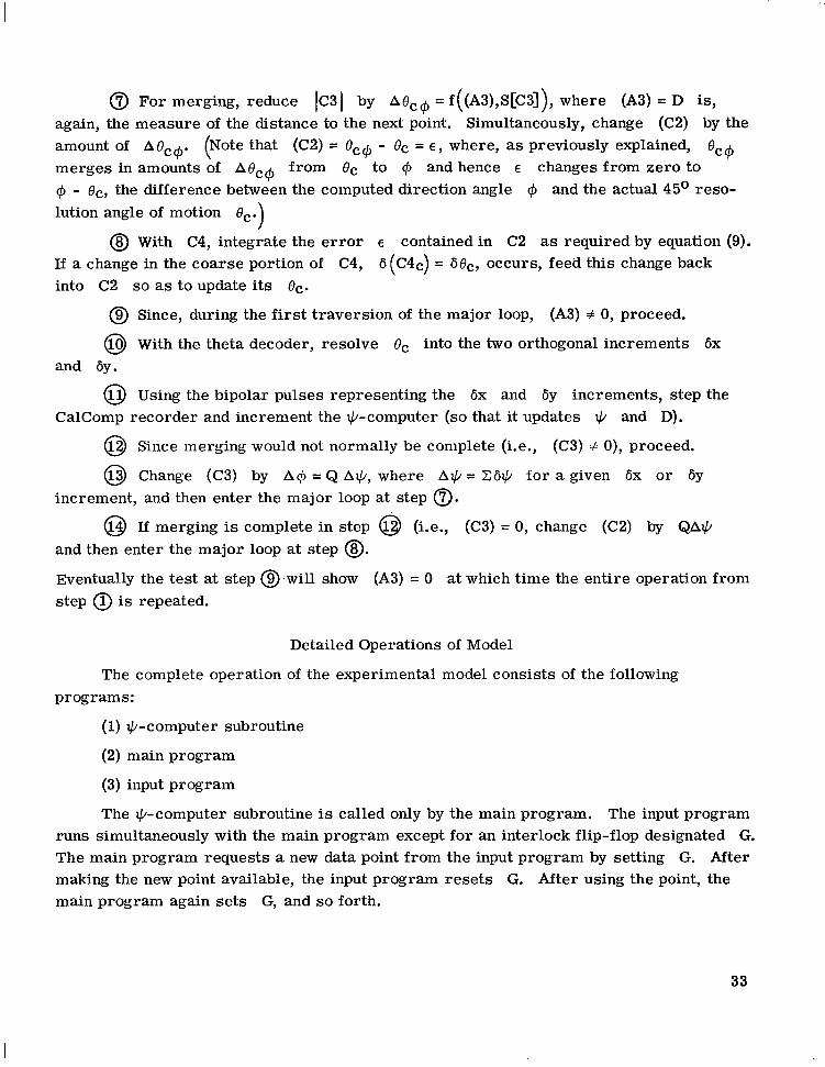
+-computer subroutine.- The +-computer, which now includes a binary rate multi- plier, is treated by the main program as a subroutine (fig. 18). It is called with the statement:

Call +-comp (6x,6y); A@) where 6x,6y increments are input arguments and A@ = Z6@, an output argument, is the total change in 4 resulting from a 6x and/or 6y ' increment.

actually exist - that is, there is no register which contains A@ = Z6@. Instead, C2 and C3 actually utilize the individual 6@ pulses. The actual representation, however, would require a transfer between the main program and the subroutine for every 6@ pulse iteration. Fortunately, this complication is eliminated by the fictitious A@ accumulator.

The quantity A@, which appears also in figure 16, is a convenience and does not

Although it is not explicit in the subroutine call statement, the main and subroutine programs can each sample the other's quantities, registers, and so forth.

Figure 18.- Symbolic implementation of +computer of model.

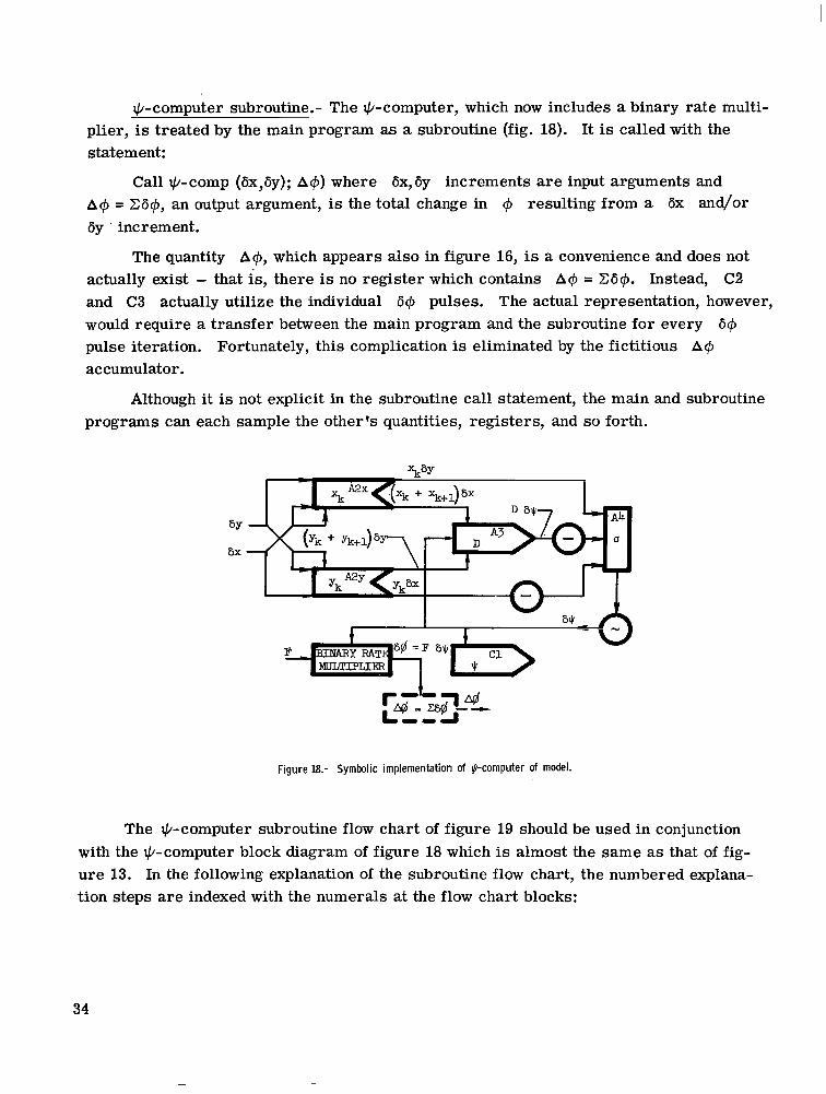
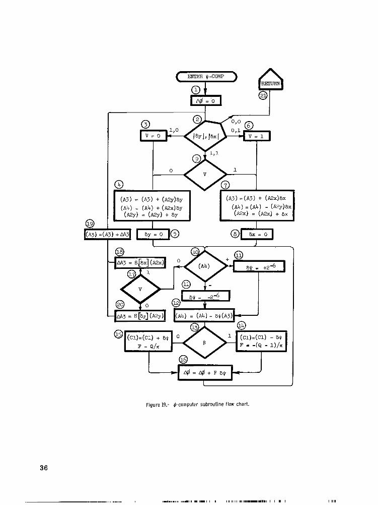
The +-computer subroutine flow chart of figure 19 should be used in conjunction with the +-computer block diagram of figure 18 which is almost the same as that of fig- ure 13. In the following explanation of the subroutine flow chart, the numbered explana- tion steps a re indexed with the numerals at the flow chart blocks:

34

@ Reset the fictitious A 4 accumulator.

@ If Idyl = 1 and 16x1 = 0, proceed.

@ Reset flip-flop V. (Flip-flop V then causes computer to operate on by.)

@ Accumulate in A3 the product of (A2y) and 6y. Accumulate in A4 the product of (A2x) and 6y. Accumulate in A2y the 6y increment.

@ Reset 6y.

@ If, in step 0, analogous manner to steps'@, @, and 0.

@ If, in step 0, go to step @; if v is set, go to step 0.

@ If (A4) # 0, proceed.

0 Assign the sign of (A4) to 61).

0 Accumulate in A4 the negative of the product of SQ and (A3).

@ If flip-flop p is set, proceed.

@ "Decrement" (See step @ on p. 32.)

@ If, in step 8, p = 0, which signifies that Q is being computed, increment

@ Accumulate in the fictitious A$ accumulator the product F 6I).

0 If (A4) = 0, proceed with step 0. If V = 1, proceed.

@ Compute AA3 = xk+16x.

@ Accumulate AA3 into (A3). Go to step 0. @ If, in step 0, V = 0, compute AA3 = yk+16y. Go to step 8. @ If 16yl = 0 and 16x1 = 0, return to the main program.

16y I = 0 and 16x1 = 1, proceed with steps @, 0, and @ in an

16yl = 1 and 16x1 = 1, proceed with step 8. If V is reset,

(p = 1 signifies that angle p is being computed. )

(Cl) by 6Q and set F = -(Q - l)/r.

(Cl) by SI) and set F = Q/r. (See step @ on p. 32.)

step @. Go to

35

(Ab) = ( A h ) - 6@(A3)'

Figure 19.- &-computer subroutine flow chart.

36

11..1.1111 , 1 1 1 1 , .I 11.1 I I IIIIIII 1111.1.111.111.1 I I I 1 I I 1 1 1

Main program.- An appreciation of the procedure used in integrating + is helpful in understanding the main program flow chart. Recall from equation (12) that it is important to keep the change in + small for incremental changes in x and y. Also, the angle + in figure 20 may be integrated by jumping from the origin to point m and then integrating to point a as was done in reference 4. This jumping avoids the singu- larity (ref. 8 ) at the origin, saves integration time, and is permissible since the path from 0 to m has no effect on +. In terms of the hardware of the experimental model, this jumping presents a problem since (A3) of the +-computer must be preset to the product xg, a quantity which, in general, is unknown. Hence, the design of the experi- mental model is based on the following integration procedure:

(1) Jump exactly 12 increments in the negative x-direction.

(2) Integrate 12 increments in y in the direction of the data point (i.e., point a in fig. 20).

(3) Integrate along the x-direction toward the point until its x-coordinate is reached.

(4) Integrate along the y-direction toward the point until its y-coordinate (and hence the point) is reached.

always to 122 = 144, and keeps the changes in + small. Such a procedure avoids the singularity at the origin, permits presetting (A3)

m

Y

Figure 20.- Integration of angle #.

37

- I

To detect when the coordinates of the point are reached as required for steps @ and @) in the integration procedure, (Alx) is decremented for each step in the x-direction and (Aly) is decremented for each step in the y-direction. A coordinate of the point is reached therefore when the associated accumulator reaches zero.

The main program flow chart of figure 21 should be used in conjunction with the experimental model hardware of figure 16. In the following explanation of the main pro- gram flow chart, the numbered explanation steps are indexed with the numerals appearing at the flow chart blocks:

0 Select the desired type of trajectory with switch Q. Set recorder to initial position, lower pen, insert paper tape, and so forth; push start.

@ Reset C3 and flip-flop L; preset U to 1 and set flip-flop G. (Flip-flop G

@ If G = 1, proceed.

@ If end of data character E has not been read on tape, go to step 0. @ If, in step 0, G = 0, which signifies RA, RB, and RC are filled, proceed

@ Increment U.

@ Set G; go to step 0. @ If, in step 0, U = 3, reset C1 and A1 and set flip-flop 0. @ Preset (Alx) to 12. (See step 0 of integration procedure.) Accumulate

interlocks the main and input programs which otherwise operate independently.)

with step 0. If U < 3, proceed.

(RAx) and -(RCx) so that (Alx) = xa - xc + 12.

@ Accumulate (RAY) and -(RCy)

@ Reset A2, A3, and A4.

0 Preset (A2x) to -12 and (A3) to x: = 122 = 144. (A2x and A3 are a part of the @-computer as shown in fig. 19. For an explanation of presetting to -12, see step @ of integration precedure.)

so that (Aly) = Ya - yc.

@ If (Aly) = Ya - yc is negative, proceed.

@ Set 6y = -1 and 6x = 0. Go to step @. @ Set J to I. GO to step 0. @ If, in step 0, (Aly) is positive, set 6y = +1 and 6x = 0. Go to step 0. 0 Decrement (Aly) by 6y and call IC/-comp (6x,6y; A+). (The @-computer

begins the integration of p.)

38

I

@ Increment (C3) by the @-computed A@ = Z6@.

@ Repeat steps 0 and @ eleven more times. (See step (2) of integration

@ If (Alx) is negative, proceed.

@ Set 6x = -1 and 6y = 0.

@ Decrement (Alx) by 6x and call @-comp (6x,6y; A@). Go to step @. @ If, in step @, (Alx) is zero, set 6x = +1 and 6y = 0. Go to step @ . @ Increment (C3) by A@.

@ through @ Treat in analogous manner to steps @ through @ . (Integra-

@ If, in step @, @ Reset flip-flop p, which signifies that @ is to be computed.

@ Preset (Alx) to -12. Accumulate (RAx) and -(RBx) so that

@ Accumulate ( M y ) and - ( m y ) so that (Aly) = Ya - yb. Go to step 0. @ H, in step @, flip-flop p is reset, set flip-flop G.

@ If IC11 > 7r, which signifies that @' is not in its principal range, proceed.

@ Set J to 402. (Note that since the weight of one 6@ pulse is '2-6 radian, 402 6@ pulses represent 27r radians. Therefore, 402 pulses (or integral multiples thereof) are used to bring @' within its principal range. 4 = (C3) is changed accordingly .)

procedure.)

tion of p is complete.)

(Aly) is zero, proceed with step @. If p = 1, proceed.

Although redundant, reset Al .

(Alx) = Xa - xb + 12.

(CI now contains - p + @ = @', the transformed angle.)

@J If (Cl) is negative, proceed.

@ Give 6@ a negative sign.

@ If J > 0, go to step @ ; otherwise, go to step @ . @ If, in step 8, (CI) is positive, give S@ a positive sign. GO to step 8. @ If, in step @, @ Decrement J. Go to step @. @ If, in step @,

J > 0, add 6@ to (Cl) and F 61) to (C3).

IC11 5 7r, proceed with step @. If U 2 3, proceed. (Q' = (Cl) has been computed and confined to its principal range and in C3.)

@ is contained

39

@ Set the coarse portion of (C4) equal to the coarse portion of (C3). Reset (C3c), leaving (C3) = @ - Bc. (Before the first portion of the curve is plotted, a reason- able initialization should be assigned to (C4;), the slope of the curve at the first point.)

@ Reset C2.

@ If (A3) > 0, proceed.

0 Decode (C4c) into its 6x and Sy components.

@ Increment the recorder with 6x and Sy.

@ Increment the +-computer with 6x and 6y.

@ If (C3) f 0, proceed.

@ Increment (C3) by A @ = Z6@ from the +-computer.

@ Increment (C2) by ABc@ = f((A3),S[C3]), the merging quantity obtained from

@ If (C3) changes sign, proceed.

@J If (C3) # 0, proceed.

@ Decrement (C2) and increment (C3) by 7r2-6 with a sign identical to s[c~]. GO to step @ .

@) If, in step @, (C3) = 0, proceed with step a. If, in step @, (C3) changes sign, proceed with step @ . Increment (C4) by (C2) and decrement (C2) by the amount of the change

the +-computer. Decrement (C3) by ABc@.

in ( ~ 4 c ) . to step @. @ If, in step @, @ If, in step @,

@ If, in step @, end of data character has been read on tape, proceed with

@ Set Z = 1. Go to step @.

@ If, in step @,

(C3) = 0, increment (C2) by A@. Go to step @. (A3) = 0, preset (C3) = -(C4c). Go to step @ to interpolate

the next segment of the curve.

step @. If Z = 0, proceed.

Z = 1, stop the operation since the complete curve is now drawn. (Note that step @ is equivalent to reading the last point twice.)

40

Figure 21.- Main program flow chart for model.

41

I -

(A21 = (A3) = (Ah) = O[

(A2x) = -12; (A3) = 144 1 I

@I

Figure 21.- Continued.

42

Figure 21.- Continued.

43

4 go 5 6 7

7 L 5x = 1; sy = -11

RECORDER (5x,5y) @c7

Figure 21.- Concluded.

44

Input program.- The input program as previously indicated operates independently of the main program except for the interlock flip-flop G which, when set by the main program, starts the input program. The flow chart of figure 22 should be used in con- junction with the input diagram of figure 23 and the tape format of table I. The following flow-chart explanation steps a r e indexed with the numerals appearing in the blocks on the flow chart:

0 If G = 0, wait; if G = 1, which signifies that the main program has requested data, proceed.

@ If model is operating in manual entry mode (i.e., not in the paper tape input mode), proceed.

LINEARLY SHIFT RA, RB, RC

.

1 J = J + 1 S C O M P L ~

0 I ~- ~

SHIFT RT, RA, RB, RC ~- _ _

-

Figure 22.- Input program flow chart of model. 45

@ Set data point into manual switches.

@ Set J = 0.

@ Shift RA, FIB, and RC in linear mode.

@ If J < 12, proceed.

0 Increment J.

@ If, in step @, J 2 12, transfer in parallel the data entry switch settings into RC (both x and y portions).

@ If, in step 0, the model is operating in the tape mode, reset tape input register

@ Read paper tape character.

@ If first tape character is a negative sign, proceed.

@ Set flip-flop S.

@ set L. GO to step @. @ If tape character of step @ is a positive sign, reset S. Go to step 8. @ Set J = 0.

T and start tape reader.

@ Shift (one step) tape input register in the circular mode.

@ Repeat step @ eleven more times.

@ Store BCD digit in least significant end of tape input register RT. Go to step @ . (Repeat steps @ through @ for next three characters which are also BCD digits. This procedure reverses the digits for the ensuing BIDEC operation.)

@ If, in step 0, character is A, set flip-flop X which connects RT to RCx.

@ Reset L which changes RT to linear shift mode.

@3J Set J = 0.

@ If quantity is negative (i.e., S = l), proceed.

@ Route quantity through two's complementing circuit.

@ If, in step @, quantity is positive (i.e., S = 0), shift (one step) RT, RA,

@ For any decade D containing a number greater than 7, proceed.

@ Decrement (D) by 3.

@ In step @, for any decade containing a number less than 8, proceed with

RB, and RC.

step @. Repeat steps @ through @ eleven more times.

46

@ ~f x = I, go to step @. @) If tape character of step 0 is a carriage return, reset X. Go to step @. @ If, in step @, X = 0, set G = 0, which indicates to main program that new

@ If, in step 0, character is E, which signifies end of tape, stop. The main program, +-computer subroutine, and input program form the basis for

data have been entered. Go to step 0.

the design of the experimental model.

0 E i

STORE COMMAM) STROBE

3 SUBTRACTER COMPLE-

REGISTER Cy I

DECECTOR selector T o main

program

G - - - - - - - I

* y-DATA &I

Figure 23.- Data entry diagram.

DESIGN OF THE EXPERIMENTAL MODEL

The discussion of the design which follows points out how the subroutine, main, and input programs are implemented in the experimental model and proceeds in this same order. The logical design, in general, is presented directly in terms of NAND modules without the AND/OR design which sometimes precedes a NAND/NOR design. No attempt is made to show pin connections, duplications of circuitry, complete integration and. con- trol circuits, and so forth; instead, included is only that portion of the design philosophy which is necessary for easy extrapolation to the complete wiring design.

Figures 24 and 25 show the logic portion of the experimental model. By use of the rack layout of figure 26 the logic for the various functions performed by INTROL can be identified. In figure 24 is a temporary panel which corresponds to location S-BLOC 4 and which will be replaced by an operation flow indicator panel when INTROL becomes fully automatic.

47

Figure 24.- Front view of INTROL logic. L-65-2367

i t i I .

Figure 25.- Rear view of INTROL rack. L-65-2369

48

COae Shift Twois

atpr 3 menter complk- detec- pulse

tor gener-

n4m ENTRY SWITCHES

INPUT REGISTERS I

x-y

er BCD/binary conversion sort-

I RF 1 I, T 1.1 i c y , T 1 1 AccurmiLator Accumulator hift pulse

generator 1

I I I I

OPERATION FLOW INDICATORS I

Controls

MASTER TIMER AND SEQTJENCER

_ _ - c3 jec,

(merging) s w

Accumulator A3

Controls Binary rate multiplier

Accumulator A4

Counter Tra. c3 jec,

(merging) s w

I Q TRAJECMRY SWITCHES

I I

Binary rate multiplier

Theta decoder

POWER SUPPLIES AND COOLING FAN

;-BLOC

1

2

3

4

5

6

7

8

9

10

Figure 26.- INlROL rack layout.

49

Design of the IC/- Computer

The *-computer occupies locations S-BLOCS 6 and 7, with its binary rate multi- plier in S-BLOC 8. Accumulators comprise a major portion of the computer. The accumulators are similar, but they do have significant differences. Therefore, a typical accumulator is described after which the peculiarities of each are pointed out.

Typical accumulator.- In general, parallel adders are considered to be faster than serial adders. In some instances, however, the well-designed parallel adder is actually slower than the serial one that is implemented with the same speed logic. For example, the serial add time per bit for 1 megacycle logic is easily 1 psec, whereas in a simple parallel adder 2.2 psec was required per stage to provide for carries. Obviously unless some provision is made perhaps to eliminate this time per stage for those stages which do not actually carry, the parallel adder is slower; to make this provision, however, greatly complicates (ref. 6) the circuit. binary type of accumulators.

Figure 27 shows a typical serial accumulator in which the quantity B is added (or subtracted if N = 1) to (or from) quantity A and the result, replacing the old value, is stored in register A. The carry (or borrow) output Pk+l is delayed one time cycle T and fed back to the input.

More typical for INTROL is the accumulator of figure 28 in which the B register is not an internal part of the accumulator and the carry (or borrow) delay is effected by the prop- agation flip-flop P.

Table I1 is a truth table for the typical accumulator. Note that the sum

for addition where N = 0 = + is Ak+l the same as for the difference for N = 1 = -. Hence, for either addi- tion or subtraction,

Ak+l

= ABP + AEP + b$ + X6P (17) Ak+l

Therefore, INTROL utilizes the serial natural

fl *E:: I pk&

I ~ I

Figure 27.- Typical serial accumulator

I 1

Ak+l = A(BP + BP) + A(BP + BP) ~~ -

Figure 28.- Typical INTROL accumulator.

50

I

where the kth subscript is implicit.

and then

Let H = BP + BP = B 0 P

= AZ + XH = A 0 H = A 0 B 0 P

(18)

(19)

Since EXCLUSIVE-OR logic was not readily available, Ak+l was implemented in the form of equation (17).

The truth table shows that the propagation signal undergoes only 4 transitions from Pk to Pk+l out of the possible 16. flop P and its simple logic which was obtained from figure 29 as

and

This fact leads to the use of flip-

- sp = NAB + NAB = B(RA + NA) = B(N 0 A) = BW (20)

'k+l ---

RP = NAB + NAE = B(RX + NA) = B(-) = BW (21) where W = N @ A. Figure 29.- Map of propagation function.

The NAND implementation of these equations is shown in figure 30.

51

Figure 30.- Implementation of propagation function.

Accumulator 3.- The accumulator of figure 28 closely represents A3 in which shift register . A is conventional (ref. 4) and comprises 24 stages. Input B is time-shared ORed with A2x and A2y outputs.

Accumulator ~- 2.- Accumulator 2, in which the x- and y-portions a r e identical, is required to perform only as a bidirectional counter in the sense that its input consists only of single plus o r minus pulses. However, since A2 must serve also as the B register for A3 and A4, it must be capable of shifting. Also, although not required in the present design, both Ak and Ak+l outputs a r e available simultaneously. There- fore, A2 is implemented as an accumulator. Its design differs from that of the typical INTROL accumulator only in that the Bk input (and associated logic) is eliminated. The counting is accomplished by setting the propagation flip-flop P and then by accumulating. Therefore, for A2, where B = 0, input equations (17), (20), and (21), respectively, reduce to

Ak+l = AF + AP

sp = 16x1 (for A2x)

and RP = Gii + NA

It is seen in figure 30 that, since Bk = 0, only the reset portion of the propagation func- tion is required for A2.

The twelve stages provided in register A enable a capacity of sign and 211 counts which are equivalent to a maximum distance of lt20.48 inches on the CalComp recorder. Since (A3) = xk 2 + YE, the maximum value of

(A3) = (211)2 + (211)2 22 22 = 2 + 2

= 223

Therefore, application

52

23 natural binary stages plus a sign stage a r e provided. actually serves only as a check since it should never indicate negative.)

(The sign bit in this

. .. . ._ _. .

Accumulator 4.- Accumulator 4 is a typical INTROL accumulator except that the For the nulling operation (eq. (14)), the nulling input is time shared by three sources.

direction is opposite to the sign of (A4) (i.e., N[A4] = S[A4]) and shall be considered complete when (A4) changes sign. This change is detected by observing the propaga- tion flip-flop P after each accumulation;,a change is implied only when P is found in the set state.

In order to establish the sign and bit weight of A4, the following symbol definitions are used:

length of (Le., number of bit positions o r stages in) RJ where J is any LRJ alphabetical character

W6U weight associated with least change in u where u is any variable or (AJ)

To accommodate need be no larger than of < lo was imposed on

A3, LA4 2 24. Since A4 is nulled after each input cycle, it A3. It is recalled that WgA3 = 2'. A resolution requirement the experimental model; hence, W6+ was made 2-6 = 0.9'.

Therefore, to accommodate A3, w6A4 5 w6A3w6+ = 20 - 2-6 = 2-6. TO accommodate

the other two inputs, w6A4 5 W6A2W6x = 2' - 20 = 20. Therefore, LA4 = 24, where six bits are located to the right of the binary point and the two inputs from A2 are scale shifted six positions as depicted in figure 31.

Figure3l.- Bk input to A4.

Shift pulse generator.- The shift pulse generator was developed to provide the set of 24 shift pulses required for operation of the accumulators. Since the accumulators operate at speeds of 1 psec, the generator has to count the set of pulses and make deci- sions at speeds approaching the upper limit of the logic used. Carry delays associated with conventional counters render such a design impractical at this speed. To minimize delays, a feedback shift register was utilized for counting. Horton (ref. 11) has shown

53

that a 12-state counter results if a 4-stage shift register is provided with Feedback = + ABE as shown in the boxed area at the top of figure 32. This arrangement gives the counting sequence of table III.

The circuitry at the bottom of figure 32 contains the necessary controls for starting and stopping the generation of pulses without pulse splitting. When SW1 is open, 12 pulses are generated as required for A1 in the input section. The operation of the controls is best shown in the timing chart of figure 33. The clock generates a 60-40 duty cycle pulse for best operation of the flip-flops. The flip- flops are clocked on the positive rise portion as indicated by the "action" line. For 12-pulse operation, the start pulse sets only M; - W and the clock then set G at the proper portion of the clock cycle to start the generation of shift pulses.

I Y Y s m Y IY I I I I 1 I \ I I

I: I

I

I I I I

I

I /

/ /

Figure 32.- Shift pulse generator.

54

I

TABLE III.- GENERATOR COUNTING SEQUENCE

State

1 2 3 4 5 6 7 8 9 10 11 12 1

Stage I

-4 1vsecP- 1Mc CLOCK

ACTION w- START - M r I r

w_ G

(a) 12 shift pulses.

CLOCK

START

M

D

!! G

SHIFT PULSE

F = % ~. \ . . - /I I

(b) 24 shift pulses.

Figure 33.- Shift-pulse-generator timing.

55

m e n 12 of these pulses are generated, the shift register returns to its original pattern of 0000; this turns on - W which immediately stops further generation. The power amplifier has three (positive logic) OR inputs and, hence, either - W or G can inhibit the generation by holding the input off.

For 24-pulse operation, SW1 is closed and, hence, the start pulse sets both D and M. When D is reset in the middle of the chain, it sets M which again effects the generation of the final 12 pulses. The gap of 2 pulses in the middle of the pulse train allows time for switching to take place in other portions of INTROL. The end of a 24-pulse operation is detected by pF, the positive transition of the signal F = DG shown in figure 33(b).

-

Counter 1.- The Src/ pulses which enter A3 are integrated by C1 so that (Cl) = ZSQ = IC/. Therefore C1 is bidirectional; it is modeled after the typical counter of figure 34. It is recalled that p = 1 and p = 0 signify that the angle being computed is angle P and angle rc/, respectively. Therefore, the C1 operation is given by

where

S[6rc/] = S[A4]

4 i I I #

#

Figure 34.- Typical bidirectional counter.

56

Controls.- The controls required to effect the sequential operations of the +-computer subroutine are explained in the form of Boolean equations. Flip-flops X, Y, Q, and E are defined, respectively, as

where MX signifies that the operation is in the X mode and F is defined in figure 33

sy= p Y I Ry = MyPF

SQ = RQ=xy

SE = PX + Py RE = P[A4]pFE

The E (error), X, and Y mode signals are, respectively, defined as

The 6+ increments a r e generated by

The shift-pulse-generator start signal is PI + I6+ I where

which can be derived from the simple function I = E + w. care of any random occurrence of 6x and 6y increments including the simultaneous occurrence. The function I is also used as

This arrangement takes

The mode signals a r e used to establish the proper operational signs and the proper interconnections for the four accumulators. Their logical equations are as follows:

N[A2x] = S[~X]

57

N[A3] = S[6x]Mx + S [6yJ My

N[A4] = S[6x]Mx + S [ ~ Y J M ~ + S[6+]ME

67 + MYS &2x]) D[SPG2] ) + M EA[A3]

Equation (27) states that the B input of A4 is connected, during the D signal (i.e., during the first 12 shift pulses (fig. 33)), to the Ak signal of A2y if the +-computer is operating in the X mode or to the Ak signal of A2x if it is operating in the Y mode, and during the 5 signal, to the appropriate A2 sign. Before entering A4, the data a r e delayed by 67 or 6 shift pulses. (See scale delay register of fig. 31.) Finally, if the +-computer is operating in the e r ro r mode in which the ffservo" is nulling, B[A4] is driven without delay by Ak of A3.

Binary rate multiplier.- As has been indicated, the binary rate multiplier (1) per- forms the Q multiplication (as required, for example, in eq. (1)) and (2) changes the angular unit of measure from radians to 71 radians (to simplify the theta decode logic). Since 71 is an irrational number and hence cannot be precisely represented in digital form, some precision must be established for its representation in the binary rate multi- plier. The resolution of II/ was set at -0.90 in the section pertaining to A4; this reso- lution represents -0.90 out of 3600 or -1 part in 400. In order not to deteriorate appreci- ably the precision limited by this resolution, Hence, the binary rate multiplier is designed to be a 10-stage device and follows the logi- cal design of figure 35 except that it is bidirectional instead of unidirectional as shown.

71 is represented to =1 part in 1000.

It is noted in figure 35 that for I input pulses, FI pulses a re emitted; IF1 is a binary number <1 - that is, Appropriate values of IFI, for various trajectories, are found in the binary columns of table IV.

IF1 = . f lf2fg . . . fn, where f . J a re binary bits.

58

TABLE 1V.- INPUT CONSTANT FOR BINARY RATE MULTIPLIER

1.00 1.25 1.50 1.75 2.00 2.25 2.50 2.75 3.00

7r

Decimal Octal Binary

.318 309 886 .2427 .010 100 010 111

.397 887 358 .3135 .011 001 011 101

.477 464 829 .3643 .011 110 100 011

.557 042 301 .4351 .lo0 011 101 001

.636 619 772 .5057 .lo1 000 101 111 -716 197 244 .5565 -101 101 110 101 .795 774 715 .6273 .110 010 111 011 .875 352 219 .7001 .111 000 000 001 .954 929 658 .7507 .111 101 000 111 1.000 000 000 1.0000 .111 111 111 111

Trajectory IFI = (Q - 1)/~

Decimal Binary I Octal

.ooo 000 000

.079 579 295 ,159 154 943 .238 732 415 ,318 309 886 .397 887 358 .477 464 829 .557 042 301 .636 619 772 .681 690 113

.oooo

.0506

.1214

.1722 ,2430 .3136 .3644 .4352 .5060 .5347

,000 000 000 000 ,000 101 000 110 ,001 010 001 100 ,001 111 010 010 ,010 100 011 000 ,011 001 011 110 ,011 110 100 100 ,100 011 101 010 ,101 000 110 000 ,101 111 100 111

Linear

Cardioid

Circular

Lemniscate Maximum

TI (pulses or pulse rate)

IF1 = .flf2f3...fn, where f are binary bits 3

Figure 35.- Binary rate multiplier.

59

Counters 2, 3, and 4.- It is seen in figure 36 that 16Q,I pulses from the binary rate multiplier go to the merging counter C3 if (C3) # 0; otherwise, the pulses go to e r ro r counter C2 which contains E = Q, - OC. Then E is integrated in C4 which contains 8 = eC + 8f. As noted in the figure any change in 8c, whether from its own S/2-l stage or from stages 22O of C2, is negatively reflected back to C2 to correct the BC portion of E.

This implementation is detailed in figure 37. It is noted that C2 differs from the typical counter of figure 34 only in that additional inputs to each stage a r e provided. When (C2) = E < 0, the value appears in two's complement notation. Therefore, since

e = CE (28)

and (C4) = 8, N[C4] = 0, always. Hence, C4 is a basic asynchronous unidirectional counter except for one change. The constraints associated with equation (28) require C4 to count or add as specified in table V. Thus the values on the left of the table a re such that 8 = 8c + Of, where 0 5 [ec _= O(mod 1 octantg < 8 and l8fl 2 0.5 octant. The right side of the table shows the corresponding binary number. This pattern is the counting sequence of a standard natural binary counter (in which p transitions of each stage

MERGING LOGIC

c2 E

c4 e

PRESET

Figure 36.- Interconnections of C2, C3, and C4. (Counter dimensional unit is octant where 1 octant = 45O.)

60

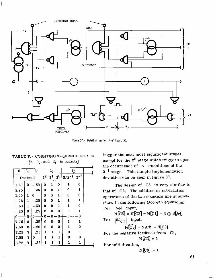
\ MERGING INPUT

ADD ?

Figure 37.- Detail of section A of figure 36.

TABLE V.- COUNTING SEQUENCE FOR C4 [e, ec, and Of in octantsl

Decimal .~

1.50 1.25 1 .oo

.75

.50

.25 0- 7.75 7.50 7.25 7.00 6.75

-

2 1 1 1 1 0 0. 0 0 7 7 7

.-

-.50 .25

1 -.25 -.. 50 .25

D - -.2E -.5c

.2! 0 -.2:

QC - -__

12 21 20 ~

~

0 1 0 0 0 1 0 0 1 0 0 1 0 0 1 0 0 0 0-0-0 0 0 0 0 0 0 1 1 1 1 1 1 1 1 1

1 0 0 1 0 0 1 1 1 0 0 1

- 0-0 1 1 1 0 0 1 0 0 1 1

5 I

c2 E

24 e

trigger the next most significant stage) except for the 2O stage which triggers upon the occurrence of a! transitions of the 2-1 stage. This simple implementation deviation can be seen in figure 37.

The design of C3 is very similar to that of C2. The addition or subtraction operations of the two counters are summa- rized in the following Boolean equations: For 1641 input,

N[C3] = N[C2] = N[Cl] = /3 @ S@4] For (6eC4( input,

N[C3] = N[C2] = S[C3] For the negative feedback from C4,

N[C2] = 1 For initialization,

N[C3] = 1 61

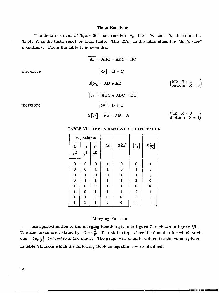
Theta Resolver

The theta resolver of figure 36 must resolve OC into 6x and Sy increments. Table VI is the theta resolver truth table. The X's in the table stand for "don't care" conditions. From the table it is seen that

therefore 16x1 = E + c

therefore

S[~X] = AB + AE

TABLE VI. - THETA RESOLVER TRUTH TABLE

ec, octants -

A

22

B

21

C

20

0 0 X 1 1 1 X 0

Merging Function

X 0 0 0 X 1 1 1

(::to: =,: = 0)

top x = 0 bottom X = 1

, An approximation to the merging function given in figure 7 is shown in figure 3.8. 2 The abscissas a r e related by D = dp. The stair steps show the domains for which vari-

OUS p c + 1 corrections are made. The graph was used to determine the values given

in table VII from which the following Boolean equations were obtained:

62

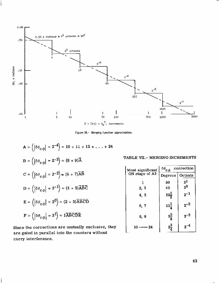
1.00

2l octants 90' - 50

1 I 5 10 50 100 500 1000

D = ( ~ 3 ) = $2, increments

Figure 38.- Merging function approximation.

A = (lae,j = 2-4) = io + 11 + 12 + . . . + 24

B = ((60c$1 = 2-3) = (8 + 9)x

C = ( (60c+( = 2-2) r: (6 + 7 ) z

--- D = (16ec+l = 2-1) = (4 + 5 ) m c

---- E = (16OC+l = 2') = (2 + 3 ) m C D

- 21 = 1XGEijii = (pecgl - )

Since the corrections are mutually exclusive, they are gated in parallel into the counters without carry interference.

5000

TABLE VII.- MERGING INCREMENTS

flost significant ON stage of A3

1 2, 3

4, 5

6, 7

8, 9

10 - 24

correction

legrees

90 45

2%

1 11- 4

8 3

s

2z

ktants

63

Input

The input section of S-BLOCS 2 and 3 of figure 26 contains the three natural binary input registers A, B, and C and the accumulator 1 which takes the various first dif- ferences among the three input points contained in the registers.

Registers.- Since RA, RB, and RC are implemented in x-y pairs, six 12-stage standard shift registers are connected as in figure 16 so that RC shifts into RB and RB into RA. This "linear" shifting enables the registers to be updated by a new input point. The registers also operate in a "circular" mode in which the serial output feeds back into the input as required by Al.

Accumulator 1.- Accumulator 1 is represented by the typical INTROL accumulator of figure 28; it has 12 stages and uses the previously described shift pulse generator (fig. 32) which is operated with SW1 open. Since RA, RB, and RC form the various serial inputs to Al, their contents must be shifted to Al. To prevent destruction of the data during this process, they are also fed back to the registers' inputs in accordance with the circular mode.

Negative quantities in the registers a r e represented in two's complement form (ref. 12) and, hence, A1 operates on these quantities just as though they were positive. Therefore, the operation of A1 for RA is always addition and for the other two reg- i s te rs is always subtraction as required for the first differences of steps @ and @ in figure 21.

Data Entry

As indicated in figure 23 two sets (12 each) of manually operated toggles a r e pro- vided for entering the x and y natural binary data. After flip-flop G 'has been reset by SW1, a main program command pulse causes the data to be transferred in parallel into RC. Since both set and reset inputs a r e connected to double-throw switches, resetting the register prior to entry is not necessary. In addition to the manual switch data entry, paper tape input is provided as an alternate mode of operation. Tape, pre- pared on the Flexowriter in the format of table I, is interpreted by a standard tape reader. Since natural binary coding is used in the input registers, the binary coded decimal (BCD) on the tape is converted to the natural binary code before entry into RC. Also, all nega- tive input points a r e converted to two's complement representation.

Code detector.- The code detector is used to recognize the non-numeric or control characters emitted by the tape reader. In INTROL these special characters serve the following functions:

64

A ''space" character which on tape separates the x- and y-data and controls flip- flop X of figure 23 which channels the x and y input data to their respective C registers

(+) and (-) sign characters which control flip-flop S that "turns on" the two's com- plementer for negative quantities

R carriage return which stops the tape reading and sets flip-flop X for next data point

Since a seven level code is utilized and only a few of the possible 27 combinations a r e used, many "don't care" conditions exist which permit a relatively simple synthesis of the detector. The particular detection codes used a r e specified in table I.

BCD to binary converter.- The BIDEC method (ref. 6) is used for the BCD to binary conversion. As related to this particular application the BIDEC algorithm is given in the section "Operations of the Experimental Model."

TABLE Vm.- TRUTH TABLE FOR "3 SUBTRACTER"

If decade reads

Binary coded decimal

0 0 0 0 0 1 0 1 1 0 1 0 1 1 1 1

Equivalent decimal number

0 to 7 8 9 10 11 12 13 14 15

Equivalent decimal number

(No change) 5 6 7 8 9 10 11 12

Change decade to

Binary coded decimal

0 0 0 1 1 1 X X

1 1 1 0 0 0 X X

0 1 1 0 1 1 0 0 0 1 1 0 X X X X

The specialized "3 subtracter" is synthesized by finding the logic which implements truth table VIII. Since counts 14 and 15 never occur, they are considered "don't care" conditions. four flip-flops of each decade is obtained:

From the reduction maps of figure 39, the following implementation for the

65

D C

B A

Figure 39.- Maps of BIDEC subtracter logic.

66

SC = DC(X +E) = DRD = pD RC = CD

Hence,

TB = AD

Hence,

It is noted that the characters a r e emitted from the tape reader with the most sig- nificant character leading and that BIDEC requires the characters to be shifted by RT of figure 23 with the least significant character leading. Since the shift register used is unidirectional, the required rearranging is accomplished as follows:

(1) Connect (with fictitious switch L) the serial output of the shift register to its serial input.

(2) Shift register 12 times.

(3) Read the BCD character, 4 bits in parallel, into the units position as shown i n figure 23.

(4) Repeat steps (2) and (3) for a total of four characters.

Since RT is 16 bits long,.its contents after reading the four characters a r e arranged as shown in figure 23. This arrangement is now ready for the BIDEC operation.

Two's comp1ementer.- If the absolute value of a negative number is subtracted from zero in the typical INTROL accumulator of figure 28, the two's complement results. Thus, since the two's complementer may be considered an accumulator in which Ak = 0 always, equations (17), (20), and (21) reduce, respectively, to

67

For the complementation of each number, P is initially reset. Equations (30) and (31) state that for complementing (Le., N = 1) P is set the first time that Bk is true in the serial operation and thereafter P remains set. Upon this hypothesis, equa- tion (29) states that for complementing, Ak+l = Bk @ 0 = Bk until the first Bk = l, after which Ak+l = Bk @ 1 = Bk. For positive numbers (Le., N = 0), P never gets set and, hence, Ak+l = Bk. Therefore, the Bk number does not get changed.

-

EXPERIMENTAL RESULTS

In general, the experimental results a r e in good agreement with the theory and confirm that the mathematical technique and implementation thereof a r e feasible. curves presented in this section a r e reproductions of those actually generated by the model and were selected because they emphasize both merits and weaknesses of the present model.

The

Evaluation of Generated Curves

The coordinates of the input data points of figure 1 were determined and read into The generated curve of figure 40 shows close agreement with the experimental model.

that of figure 1.

Y

0 100 200 400

Figure 40.- Points of f igure 1 interpolated by experimental model.

68

Y .c

Figure 41.- The f igure eight.

A considerably more difficult task is exhibited in figure 41. The figure-eight curve

demonstrates the ability to

(1) draw smooth curves through widely spaced points

(2) operate on nonequal argument data

(3) produce multivalued functions

(4) process data in all four quadrants

(5) handle infinite tangents

(6) produce both positive and negative rotations

At first glance, the curve between points 8 and 9 appears to be in error . the point sequence indicated in the figure is carefully considered, the distorted shape is found to be a reasonable interpolation.

The.curve between points 8 and 9, however, does reveal a weakness of the experi-

However, when

mental model. The abruptness in the turning is a result of the inability of its merging hardware to handle effectively any points which a r e spaced >0.7 inch. ever, is easily extended by adding similar stages of logic.

This range, how-

69

Figure 42.- Merging examples.

Y

X

, -100)

Figure 43.- Circle through two pofnts and one slope.

Figure 42 shows some results of merging tests designed to insure satisfactory merging in all directions. The point separation of -0.7 inch was chosen since, as previously mentioned, this distance represents the maximum effective merging range for the model.

As predicted in the section "Derivation of Output Function," the circle of figure 43 does have four sides slightly flattened. It is recalled that this tendency to flatten results from a mathematical approximation and that for normal curve interpola- tion this flatness is insignificant. This particular circle was drawn clockwise, first from A to B and then from B to A. In addition to the

70

. .. . . ..... -. .. ..

coordinates of A and B, the input data included the slope at B for the A to B portion and the slope at A for the B to A portion.

The curves in figures 40 to 43 were generated in the circular mode. The cardioid mode is demonstrated in figure 44. The curve was generated first from A to B over the lower path and then from A to B over the upper path. The input data consisted of the coordinates of A with respect to a coordinate system centered at B and alined with the slope (zero) of B. The upper or lower path is selected by integrating IC/ over a path in the upper or lower half-plane, respectively. An explanation of this selection can be seen in basic equation (l),

4' = &IC/'

by observing the initial $I' for both IC/ = +T and IC/ = -T. Furthermore, since d@' = Q dIC/' and Q > 0, the sense of rotation of 4' is the same as that of IC/'. In general, then, as a point moves along the interpolated path, IIC/'l and 14'1 = Q decrease monotonically, both ending with zero slope.

Careful inspection of this cardioid curve and the circular curve reveals a slight discrepancy in symmetry. (ref. 6) in the binary rate multiplier. this symmetry, as perhaps in the control of a machine tool, two or three stages of smoothing are recommended. A secondary contributor to the distortion may be the coarse resolution in several components of the system where, in the interest of simple

This distortion results primarily from the lack of smoothing For applications in which it is important to correct

Y

Figure 44.- Cardioid through two points and one slope.

71

and minimal hardware, the model was designed with fewest stages. For example, some of the computations are resolved to only -3O. In some applications, however, this resolu- tion should be extended by a factor 24.

Finally, the lemniscate mode is demonstrated by the curve of figure 45. Again two points and one slope dictated the path which was drawn. It is noted that the entire path lies in the same quadrant with the starting point A. The Y-axis then represents an unstable line on which the lemniscate diverges. Thus l+'l must be limited to ~ / 2 .

-75 1

X

Figure 45.- Lemniscate through two points and one slope.

+' Boundaries

In general, the +' limit occurs when ]+'I reaches a value such that I@' - +'I = T. This limit may be stated as a function of Q as follows:

T > 16' - + ' I = IQ+' - +'I = J+'(Q - 111

For Q > 1,

and, therefore,

To cover all four quadrants, +' must range over 27r. This range can be effected with a maximum value of I + ' I gives

of T. Substituting this maximum value in equation (32)

72

Hence,

and, therefore,

Thus, any two points in the finite coordinate system can be connected and termi- nated with any prescribed slope if 1 < Q < 2. Note that the interval is open. Therefore, for the important circular mode in which Q = 2, an unstable though somewhat trivial domain exists: the line for which +' = fa.

@-Computer Error

It is recalled that the design of the +-computer is based on the approximation S q = tan S q . Near the origin, however, 45' angle would be computed as ~ 5 7 ~ . This discrepancy of 12' is prohibitive. In the model, it w a s reduced to an e r ro r of <lo simply by presetting accumulator A3 to 0.012 before the computation of each angle.

S+ can be as great as 45O per increment; this

Initialization of (C3)

In step @ of the operations algorithm (p. 32), each new segment 2 of interpola- tion is initialized to -ec, the angle at which the last step entered a data point. In general, this angle is not p2 the "average" slope of the (2 - 1)th segment into the point. Since the initialization should be 0, -1 and not ec, prohibitive angular discontinuities result. Therefore, for the curves in figures 40 and 41 each initialization was manually adjusted to pZel when lec - pz -11 was large.

The correct initialization may be implemented by using C1 which contains, at the end of a segment, a measure of the desired angle is radians and, hence, the quantity must be counted into the binary rate multiplier for con- version to P radians and then recounted into C3. Step @ of the operations algorithm is corrected by the following procedure:

p2 -l. Unfortunately the unit of (Cl)

@ Reset C2 and C3.

@ Set ( ~ 2 ) = - ( ~ 4 ~ ) .

@ Count-down (Cl) through the binary rate multiplier into both C2 and C3 and apply appropriate multiplying factor and operational signs to leave (C2) = PI -1 - BC

and (C3) = -p2 -l.

@ Integrate @ and simultaneously count the angle into C3 to leave (C3) = - P2-1.

@ Begin the interpolated segment.

73

RESEARCH BYPRODUCTS

During the development of the subject controller, several innovations or research byproducts ensued. These byproducts are essentially separate entities which should find application in other areas, devices, or systems. The most important byproducts are as follows :

+-computer: A special purpose incremental digital computer for integrating the arc tangent angle as a function of various finite Sx and Sy input increments The described design can be easily modified to obtain virtually any accuracy and capacity. If the +-computer is utilized as a finite difference device, its speed is great.

Bidirectional binary rate multiplier: A device which eliminates the "hysteresis" inher- ent in conventional binary rate multipliers when utilized in bidirectional applications

Adder with round off: A digital accumulator which outputs rounded-off information to one precision but retains a finer precision for subsequent calculations Although developed in a natural binary system, the scheme is applicable to other weighted codes provided only that the weight of the least significant bit of the rounded portion is twice that of the adjacent lower order bit which, on turning on, carr ies into it. For example, in a BCD code of weight 1-2-4-5, the least significant bit (bit 1) of one decade has twice the weight as that of the most significant bit (bit 5) of the adjacent lower order decade; hence such a code is suitable.

High speed shift pulse generator: A device which, on command, generates a fixed number of fully formed pulses at a rate equal to the nominal speed of the logic with which it is implemented Although developed with the fixed number as 24, the scheme is adaptable to virtually any quantity.

Serial two's complementer: A simple digital device for serially converting a sign- magnitude negative number to its two's complement representation (and vice versa)

NEED FOR ADDITIONAL RESEARCH

The experimental results indicate that the merging-function-constant-Q concept developed in this research works well. Nevertheless, the concept was an expediency which does not f i t harmoniously into the system. Therefore, the scheme which follows seeks to satisfy this need.

From the fundamental relation @ ' = w' (eq. (l)),

74

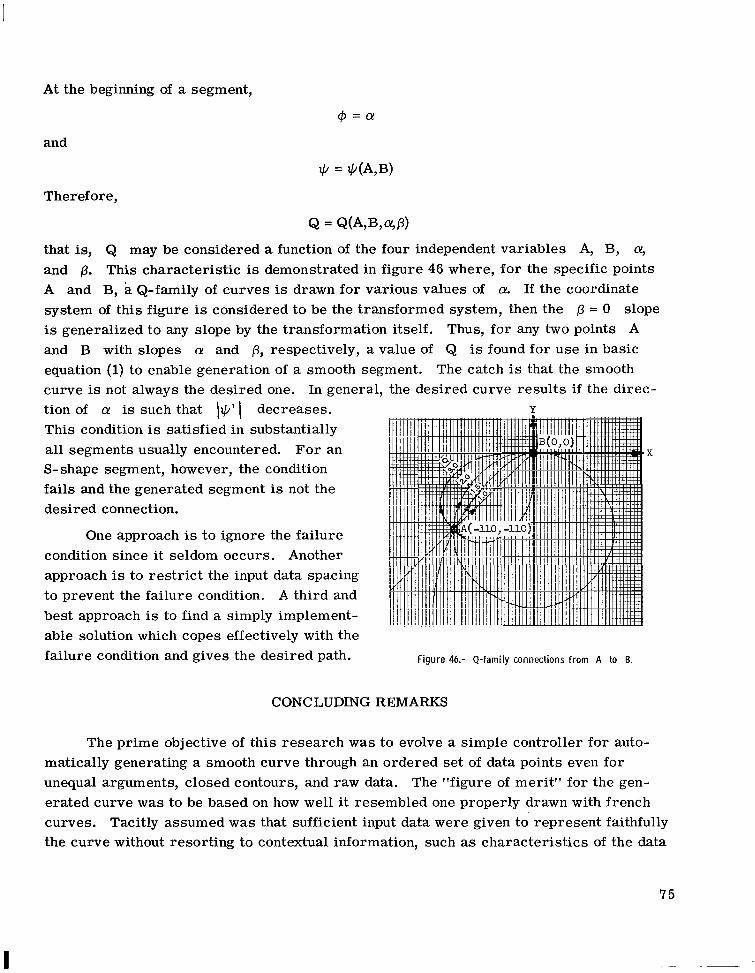
At the beginning of a segment,

@ = a !

and

IC/ = IC/(A,B)

Therefore,

Q = Q(A,B,M)

that is, Q may be considered a function of the four independent variables A, B, a, and p. This characteristic is demonstrated in figure 46 where, for the specific points A and B, a Q-family of curves is drawn for various values of a If the coordinate system of this figure is considered to be the transformed system, then the p = 0 slope is generalized to any slope by the transformation itself. Thus, for any two points A and B with slopes CY and p, respectively, a value of Q is found for use in basic equation (1) to enable generation of a smooth segment. The catch is that the smooth curve is not always the desired one. In general, the desired curve results if the direc-

This condition is satisfied in substantially

S-shape segment, however, the condition fails and the generated segment is not the desired connection.

tion of a! is such that \IC/' I decreases. Y

all segments usually encountered. For an X

One approach is to ignore the failure condition since it seldom occurs. Another approach is to restrict the input data spacing to prevent the failure condition. A third and best approach is to find a simply implement- able solution which copes effectively with the failure condition and gives the desired path. Figure 46.- Q-family connections from A to B.

CONCLUDING REMARKS

The prime objective of this research was to evolve a simple controller for auto- matically generating a smooth curve through an ordered set of data points even for unequal arguments, closed contours, and raw data. The "figure of merit'' for the gen- erated curve was to be based on how well it resembled one properly drawn with french curves. Tacitly assumed was that sufficient input data were given to' represent faithfully the curve without resorting to contextual information, such as characteristics of the data

75

I

I

source (e.g., frequency content, bandwidths, o r intentional discontinuities), or recognizing that the input data f a l l into some analytic function or geometric shape. The effect of context was forcibly demonstrated when the figure eight was redrawn in the context of two circles; the resulting curve was significantly less distorted. eight the sufficient input data assumption was violated. The foregoing and other experi- mental curves do indicate that given sufficient input data, the controller generates curves of equal fidelity to the skilled draftsman using french curves. Another way of stating this fact is: if enough input data are given so that the same curve results when drawn (out of context) by several skilled draftsmen, then the controller will also produce the same curve. highly subjective interpretation is perfectly adequate if consistently applied to both draftsmen and controller.

Therefore, for the figure

The word "same" does not require a quantitative definition because even a

Considering the magnitude of the task which it performs, the controller satisfies also the secondary objectives of simplicity and speed.

Langley Research Center, National Aeronautics and Space Administration,

Langley Station, Hampton, Va., April 6, 1966.

76

APPENDIX

X-axis reference direction does not change; hence + is invariant. However, under coordinate rotation (from system 2 to sys- tem 3), the reference direction changes by the amount of the rotation; hence + changes by an equal amount and, thus

Y1

b

/

DERIVATION OF STEERING ANGLE 4

3 X

$'

P x2

Consider the present problem to be that of determining the angle $' associated with the tangent of figure 2. The angle 4' can then be transformed to $ which can be used to guide point p from a to b.

Since b' is a destination of p' , the direction of b' with respect to p' is apparently an important parameter. The angle +' is therefore defined, as indicated in figure 2, as the instantaneous angle of the line connecting b' and p' as p' moves along the curve - that is,

where x' and y' are the coordinates of p'.

77

APPENDIX

Let cp' = cp'(t,b') and, in the interest of obtaining simple relationships, assume that

(es. (1)) $ 1 = Qq'

where Q is a constant. Several significant cases then result.

Case I - Q = 1: Obviously case I is the linear case in which

where c is a constant for xk 5 x' < x;. Hence @' would guide p' over a constant slope or linear path from a' to b'.

Case 11 - Q = 2: From equation (l),

cp' = 2t,b' dY In figure 2 it is seen that - = tan @'. dx Therefore,

a first order, homogeneous differential equation. (Prime with x and y is implicit.) Let

Y v = - X

then y =vx and

Separating the variables gives

3 --

2 v - v + v dx dv dv(1 - v ) ~

2v v - -- x - 1 - 4 -

Therefore,

v v + 1 ".w X

By use of partial fractions,

(37)

2 A B 1 - v +- V(v2+.=7 v 2 + 1

78

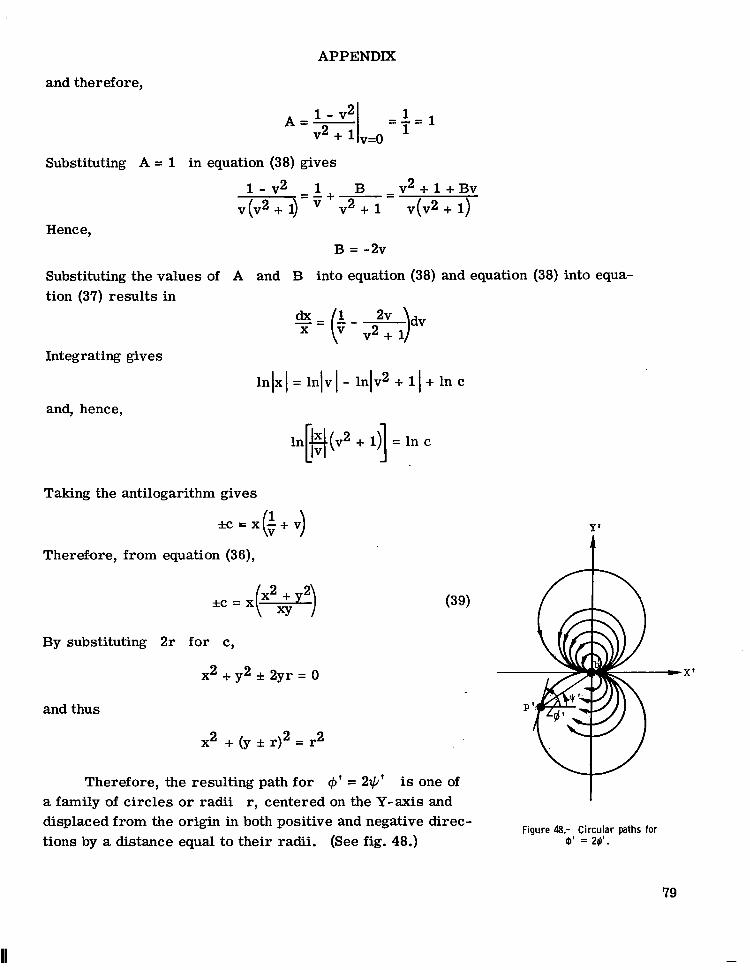
APPENDIX

and therefore,

1

Substituting A = 1 in equation (38) gives

1 - v 2 1 B - v 2 + 1 + B v

Hence, B = - 2 ~

Substituting the values of A and B into equation (38) and equation (38) into equa- tion (37) results in

Integrating gives

lnlxl= 1nJvl- lnlv2 + 11 + In c

and, hence,

Taking the antilogarithm gives

*C = x g + v)

Therefore, from equation (36),

By substituting 2 r for c,

x 2 + y 2 * 2 y r = o

and thus

x2 + (y * r)2 = r 2

Therefore, the resulting path for $' = 2q ' is one of

Y'

t

X'

I a family of circles o r radii r, centered on the Y-axis and displaced from the origin in both positive and negative direc- tions by a distance equal to their radii. (See fig. 48.)

Figure 48.- Circular paths for $' = 2#'.

79

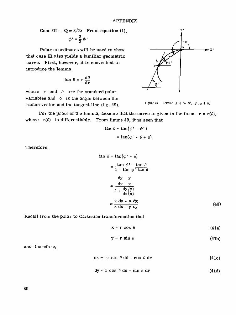
APPENDIX

Case III - Q = 3/2: From equation (l), Y' A 3

@' = z V -e b

Polar coordinates will be used to show that case III also yields a familiar geometric curve. First, however, it is convenient to introduce the lemma

7 X'

de t a n 6 = r - dr

where r and 8 a r e the standard polar variables and 6 is the angle between the radius vector and the tangent line (fig. 49).

/

Figure 49.- Relation of 6 to O', $', and 0.

For the proof of the lemma, assume that the curve is given in the form r = r(e), where r(e) is differentiable. From figure 49, it is seen that

tan 6 = tan(@? - tc/') = tan(@? - e + T )

Therefore,

tan 6 = tan(@' - e) - tan @ ? - tan 8

1 + tan @' tan e -

9-'

Recall from the polar to Cartesian transformation that

x = r COS e

y = r sin 8

and, therefore,

dx = -r sin e dB + cos e dr

dy = r cos 8 de + sin 8 dr

80

APPENDIX

Substituting equations (4 1) into equation (40) gives

tan 6 =

- -

which proves the

r cos e(r cos e de + sin 8 dr) - r sin e(-r sin 8 de + cos 8 dr) r cos e(-r sin 8 de + cos 8 dr) + r sin e(r cos 8 de + sin 8 dr)

r2cos2e de + r2sin20 de - r2de dB r cos2e dr + r sin2f3 d r r d r dr

--=r-

lemma. From this lemma and figure 49,

de dr r -- = tan 6 = tan(rC/?/Z) = tan

Separating the variables results in

d r de = sin(B/2)de ~0t(e/2) COS( e/2)

-= -

Since the numerator is the differential of the

the right-hand side) equation (42) is easily denominator (except for a factor of 1/2 on Y'

integrated to give

X'

In r = 2 In COS(^/^) + In 2a

where r > 0, cos(O/2) >O, a >O, and In 2a is the integration constant. Taking the antilogarithm gives

r = 2a ~ 0 ~ 2 ( e / 2 ) (-71 < e < a)

a n 4 therefore,

r = a(l + cos e) (43) I

Figure 50.- Cardioid for @' =: #' . the classical form of the cardioid of figure 50.

Case IV - Q = 3: From equation (l),

4' = 3Ip

Again, from the lemma and figure 49,

r - de = tan 6 = tan(2(8 - 71)) = tan 28 d r

81

APPENDIX

Separating the variables results in Y'

I dr de (cos 28)de r t an28 sin 28 -=-=

which is easily integrated to give

1 2

In r = - ln(sin 26) + In a

where r > 0, sin 28 > 0, a > 0 (fig. 51), and In a is the integration constant. Taking the antilogarithm yields

r2 = a2sin 20 (4 5)

the classical form of the lemniscate (ref. 13) of figure 51.

(44)

Figure 51.- Lemniscate for 0' = 3 ~ ' .

Since most of the equations of the foregoing figures are recognizable more easily- in polar coordinates, a polar generalization, which includes cases I1 to IV (case I is con- sidered to be trivial), is now derived. The relations

and

from figure 49 with equation (1)

give

Therefore the lemma can be expressed as

6 = $ 7 - *c . '

+ f = e - ~

$ 7 = Qq'

6 = (Q - l ) ( O - T)

r - d8 = tan[(Q - l ) ( O - T) + rk] d r

where k is any integer. Separating the variables results in

d r cos[(Q - l ) (8 - T) + Tk]d8

sin[(Q - l)(8 - T) + ~4 - =

which is easily integrated to give

l n r = - In sin[(Q - l ) ( O - T) + ~ f l + - l n c Q - 1 Q - 1

1 Q - 1

where r > 0, sin[(Q - l)(8 - T) + Tk] > 0, c > 0, and - In c is the integration

constant. Taking the antilogarithm yields the polar generalization

X'

82

APPENDIX

rQ-' = c sin[(Q - l ) ( e - n) + nk]

where the domains of 8 result from the conditions that

(sinC(Q - l ) ( e - T ) + ~k] > 0) *(O + 27rm < [cQ - l ) (e - n) + nk] < 7~ + 2nm)

for any integer m, and 2nm c kn.

For case 11, in which Q = 2, equation (46) becomes for k = 1

r = c sin 8

r = -c sin 8

(0 < e < 9)

(n < e < 2n) and for k = 0

which agrees with equation (39), as can be seen from the following transformation to Cartesian coordinates:

2 2 *c=-=- r l-2 - x + Y sin e r sin 6 Y

For case 111, in which Q = 3/2, equation (46) becomes for k = 1

Squaring both sides gives

r = c2cos2(:) = c2 +(I + cos e)

C2 which agrees with equation (43), where - = a. 2

For case IV, in which Q = 3, equation (46) becomes for k = 2 and k = 0, respectively,

r2 = c sin 2e (."::;) which agrees with equation (45), where c = a2. Also for k = 1 and k = -1, respectively,

r2 = -c sin 2e (.<<:<::)

83

APPENDIX

Thus, equation (46) becomes

r Q-l = c sin[(Q - 1)8]

for integer values of Q > 0 and for k = Q - 1, and

= ~ ' { l + COS[~(Q - 1)4}

2 for integer values of (Q + 0.5) > 1 and for k = Q - 0.5 and c' = - 2 '

C

(47)

Other popular geometric shapes can probably be found by solving equation (47) for additional integer values of Q or solving equation (48) for additional "half-integer" values. Also, Q may be quartered or further subdivided to obtain other shapes. With- out attempting to exhaust all of the important shapes, however, a significant conclusion is stated in the following theorem which is based on figure 49:

Theorem: If 8 is the polar angle of a point on a curve and $I is the tangent angle of the curve at the point, then for -a S (+ = 8 - a) < a simple linear relationships exist between $I and +, such that p generates smooth well-known geometric shapes which go through the coordinate origin at zero slope.

All that remains to be proved is the origin zero-slope portion. That the origin is a solution of equation (46) is easily seen by substitution; its slope may be determined as follows:

lim rQ-l = 0 = lim c sin[(Q - l ) ( O - a) + rk] P-0 P-0

where p - 0 means "as point p approaches the origin." Therefore,

lim KQ - l)(8 - a) -t- ak] = am P-0

where m is any integer. Letting m = k gives

and since (Q - 1) # 0 lim e = n P-0

Therefore, the curve goes through the origin at zero slope.

84

REFERENCES

1. Mergler, Harry Winston: A Numerical Machine Tool Control System Operating From Coded Punched-Paper Tape. Publ. No. 20,943, Univ. Microfilms, Inc., 1956.

Control Eng., 2. Henegar, H. B.: New Continuous Path System U s e s DDA Interpolator. vol. 8, no. 1, Jan. 1961, pp. 71-76.

3. Kaiwa, Toshimasa; and Inaba, Seiuemon: Latest Japanese Numerical Control Features. Control Eng., vol. 8, no. 10, 1961, pp. 88-91.

4. Batte, William Granville: A Digital Higher Order Interpolation Path Controller. Ph.D. Thesis, Case Inst. Technol., 1965.

5. Ninke, William H. : A Two- Dimensional Absolute Digital Data Path Control System. Rept. No. EDC- 1-63- 18 (NsG-36-60), Digital Systems Lab., Case Inst. Technol., Sept. 1963.

6. (Mergler, H. W.]: Notes on Digital Control Systems Engineering. Vols. 1 and 2, Eng. Div. of Case Inst. Technol.

7. Goldberg, Samuel: Introduction to Difference Equations.

8. Kaplan, Wilfred: Advanced Calculus. Addison-Wesley Press , Inc., 1952.

9. Ledley, Robert Steven: Programming and Utilizing Digital Computers. McGraw-Hill

Sci. Eds., Inc., 1961.

Book Co., Inc., c.1962, pp. 127-132.

10. Lee, Thad; and Mix, Gerhart: TRICE Lecture Notes. CSP-156, Packard Bell Computer, Sept. 1963.

11. Horton, William P.: Shift Counters.

12. Phister, Montgomery, Jr.:

3C 013-6, Computer Control Co., Inc.

Logical Design of Digital Computers. John Wiley & Sons, Inc., c.1958.

13. Burington, Richard Stevens: Handbook of Mathematical Tables and Formulas. Fourth ed., McGraw-Hill Book Co., c.1965.

NASA-Langley, 1966 L-4736 85

“The aeronautical and space activities of the United States shall be conducted so as t o contribute . . . to the expansion of human knowl- edge of phenomena in the atmosphere and space. shall provide for the widest practicable and appropriate dissemination of information concerning its activities and the results thereof .”

The Administration ,

-NATIONAL AERONAUTICS AND SPACE ACT OF 1958.

! NASA SCIENTIFIC A N D TECHNICAL PUBLICATIONS

TECHNICAL REPORTS: Scientific and technical information considered . important, complete, and a lasting contribution to existing knowledge.

TECHNICAL NOTES: of importance as a contribution to existing knowledge. .

TECHNICAL MEMORANDUMS: Information receivibg limited distri- bution because of preliminary data, security classification, or other reasons.

CONTRACTOR REPORTS: Technical information generated in con- nection with a NASA contract or grant and released under NASA auspices.

TECHNICAL TRANSLATIONS: Information published in a foreign language considered to merit NASA distribution in English.

TECHNICAL REPRINTS: Information derived from NASA activities and initially published in the form of journal articles.

SPECIAL PUBLICATIONS: Information derived from or of value to NASA activities but not necessarily reporting the results of individual NASA-programmed scientific efforts. Publications include conference proceedings, monographs, data compilations, handbooks, sourcebooks, and special bibliographies.

Information less broad in scope but nevertheless

. ,

I

L

Details on the availability of these publications may be obtained from:

\:* SCIENTIFIC AND TECHNICAL INFORMATION DIVISION

N AT1 0 N A L A E R 0 N A UTI CS A N D S PAC E A D M I N I ST RAT I 0 N

Washington, D.C. PO546