NBER WORKING PAPER SERIES

THE EXTENSIVE MARGIN OF EXPORTING PRODUCTS:A FIRM-LEVEL ANALYSIS

Costas ArkolakisMarc-Andreas Muendler

Working Paper 16641http://www.nber.org/papers/w16641

NATIONAL BUREAU OF ECONOMIC RESEARCH1050 Massachusetts Avenue

Cambridge, MA 02138December 2010

We thank David Atkin, Thomas Chaney, Arnaud Costinot, Don Davis, Gilles Duranton, JonathanEaton, Elhanan Helpman, Kalina Manova, Gordon Hanson, Lorenzo Caliendo, Sam Kortum, GiovanniMaggi, Marc Melitz, Peter Neary, Jim Rauch, Steve Redding, Kim Ruhl, Peter Schott, Daniel Treflerand Jon Vogel as well as several seminar and conference participants for helpful comments and discussions.Roberto Avarez kindly shared Chilean exporter and product data for the year 2000, for which we reportcomparable results to our Brazilian findings in an online Data Appendix at URL econ.ucsd.edu/muendler/research.We present an extension of our model to nested CES in an online Technical Appendix at the sameURL. Oana Hirakawa and Olga Timoshenko provided excellent research assistance. Muendler andArkolakis acknowledge NSF support (SES-0550699 and SES-0921673) with gratitude. A part of thispaper was written while Arkolakis visited the University of Chicago, whose hospitality is gratefullyacknowledged. The views expressed herein are those of the authors and do not necessarily reflect theviews of the National Bureau of Economic Research.

NBER working papers are circulated for discussion and comment purposes. They have not been peer-reviewed or been subject to the review by the NBER Board of Directors that accompanies officialNBER publications.

© 2010 by Costas Arkolakis and Marc-Andreas Muendler. All rights reserved. Short sections of text,not to exceed two paragraphs, may be quoted without explicit permission provided that full credit,including © notice, is given to the source.

The Extensive Margin of Exporting Products: A Firm-level AnalysisCostas Arkolakis and Marc-Andreas MuendlerNBER Working Paper No. 16641December 2010JEL No. F12,F14,L11

ABSTRACT

We use a panel of Brazilian exporters, their products, and destination markets to document a set ofregularities for multi-product exporters: (i) few top-selling products account for the bulk of a firm'sexports in a market, (ii) the distribution of exporter scope (the number of products per firm in a market)is similar across markets, and (iii) within each market, exporter scope is positively associated withaverage sales per product. Our data also show that firms systematically export their highest-sales productsacross multiple destinations. To account for these regularities, we develop a model of firm-productheterogeneity with entry costs that depend on exporter scope. Estimating this model for the within-firmsales distribution we identify the nature and components of product entry costs. We find that firmsface a strong decline in product sales with scope but also that market-specific entry costs drop fast.Counterfactual experiments with globally falling entry costs indicate that a large share of the simulatedincrease in trade is attributable to declines in the firm's entry cost for the first product.

Costas ArkolakisDepartment of EconomicsYale University, 28 Hillhouse AvenueP.O. Box 208268New Haven, CT 06520-8268and NBERcostas.arkolakis@yale.edu

Marc-Andreas MuendlerDepartment of Economics, 0508University of California, San Diego9500 Gilman DriveLa Jolla, CA 92093-0508and NBERmuendler@ucsd.edu

An online appendix is available at:http://www.nber.org/data-appendix/w16641

1 Introduction

Market-specific entry costs are an important ingredient in recent trade theory. Combined with firm

heterogeneity, entry costs serve as a key explanation for exporter behavior and the size distribution

of firms.1 After rounds of tariff reductions and drops in transport costs, local entry costs from

technical barriers to trade and regulatory protection are thought to be major remaining impediments

to trade (Baldwin 2000, Maskus and Wilson 2001).2 Micro-econometric estimates suggest that

firm entry costs are a substantive fraction of export sales (Das, Roberts, and Tybout 2007, Maskus,

Otsuki, and Wilson 2005). Market-specific fixed costs do not only limit firm entry, they also hinder

the expansion of prolific multi-product exporters.

To study the nature and components of entry costs, we use comprehensive data on multi-

product firms and their destinations. Beyond the extensive margin of firm presence, we decom-

pose, destination by destination, an exporter’s sales into the extensive margin of the number of

products—the exporter scope—and the remaining intensive margin of the exporter’s average sales

per product, which we call exporter scale. We use a structural approach to quantify the relevance

of multi-product exporters in a general-equilibrium framework for the first time. To do so, we

separately identify sources of within-firm heterogeneity in product sales and economies of scope

in local product entry costs. Based on our estimates, we assess the general-equilibrium effects of

reduced market-specific fixed costs on the expansion of incumbent multi-product exporters and

new exporters. Our simulations suggest that new products of incumbent exporters contribute less

to bilateral trade than new exporters.

A number of key regularities emerge from our Brazilian exporter data and discipline the anal-

ysis.3 First, a few top-selling products explain the bulk of a firm’s exports in a market, whereas

wide-scope exporters sell their lowest-selling products in minor amounts.4 Second, within des-

1See for example Melitz (2003), Chaney (2008) and Eaton, Kortum, and Kramarz (2010).2The World Bank estimates in its Global Economic Prospects 2004 report that trade facilitation would increase

world trade by approximately $377 billion overall, to which an improvement in the regulatory environment wouldcontribute $83 billion and services sector infrastructure and e-business usage another $154 billion (World Bank 2003).The World Trade Organization’s World Trade Report 2008 asserts that “with respect to product standards, technicalregulations and sanitary and phytosanitary (SPS) measures, considerable opportunities exist for reducing trade costs”(WTO 2008, p. 149).

3To assess robustness for another country, we use panel data of Chilean exporters in 2000 (see Alvarez, Faruq,and Lopez 2007). We find the regularities confirmed and estimates to be similar, and report them in our online DataAppendix.

4Bernard, Redding, and Schott (2010a) document a similar pattern for worldwide shipments by U.S. firms. Weshow that the pattern is repeated market by market.

1

tinations, there are few wide-scope and large-sales firms but many narrow-scope and small-sales

firms. Third, within destinations, mean exporter scope and mean exporter scale are positively as-

sociated. These three regularities occur repeatedly destination by destination. Comparing across

destinations but within firms, we find that exporters are likely to sell their highly successful prod-

ucts in many destinations and in large amounts. We interpret this body of regularities as evidence

of heterogeneity in product efficiency, or consumer appeal, and as evidence of entry costs that vary

by product and destination.

Guided by these facts, we propose a model of firm-product heterogeneity where firms face

destination-specific entry costs for each of their products. The model rests on a single source of

firm heterogeneity (productivity) and firms face declining efficiency in supplying their less suc-

cessful products, similar to Eckel and Neary (2010) and Mayer, Melitz, and Ottaviano (2009).5

Our specification of local entry costs accommodates the cases of both economies or diseconomies

of scope.6 The setup offers a tractable extension of the Melitz (2003) framework to multiple prod-

ucts where the firm decides along three export margins: its presence at export destinations, its

exporter scope at a destination, and its individual product sales at the destination.

We use our model’s structural implications to obtain novel estimates for parameters that govern

separate entry cost components, fitting the within-firm heterogeneity under the first regularity.

We check the fitted model’s prediction for the remaining two regularities across firms and show

that the model approximates well the scope and sales distributions and generates the observed

positive association between exporter scope and exporter scale. Estimates point to a strong decline

in product efficiency with scope. So only highly productive firms choose a wide scope. But

local entry costs exhibit economies of scope for the introduction of additional products within

a market, consistent with the fact that wide-scope exporters sell their lowest-selling products in

minor amounts.

Having parameterized the model, we simulate a 25-percent reduction in entry costs and their

effect on global trade. We distinguish between a decline in firm entry costs for the first product

and a decline in entry costs that a multi-product exporter incurs for additional export products. We

5Bernard, Redding, and Schott (2010a) develop a multi-product firm model with products that have idiosyncraticcountry-specific demand shocks. Departing from CES demand, Eckel, Iacovone, Javorcik, and Neary (2010) studythe firm’s investment in product appeal. Exporter scope is socially optimal in these models. Thomas (2010) proposesan agency approach to product adoption and documents inefficient variation in firm scope for detergent manufacturersacross local markets in Western Europe.

6Seminal references on economies of scope are Panzar and Willig (1977) and (1981). Formally, there are economiesof scope if the cost function satisfies C(x+ y) < C(x) + C(y) (if the cost function is subadditive).

2

find that most of the simulated trade increase is due to falling entry costs for the first product—

such as one-shot startup costs for information acquisition, the setup of certified and accredited

testing facilities, investments in technology acquisition for export development, and perhaps brand

marketing costs. In contrast, trade is less sensitive to falling entry costs for subsequent products—

such as compliance with an individual product’s technical requirements, mandatory or voluntary

product safety standards, and packaging and labelling procedures, or expenditures for extending

marketing and the distribution network to additional products.

Overall, a simulated 25-percent reduction in entry costs only results in a less than 1-percent

welfare increase. Firm entry costs are typically found to influence sales little because only small

exporters around the entry threshold respond (Das, Roberts, and Tybout 2007, di Giovanni and

Levchenko 2010). But incumbent exporters add products when entry costs fall, suggesting poten-

tially salient changes to trade flows because multi-product exporters dominate trade. Our simula-

tions show, however, that the elasticity of trade with respect to product entry costs is even smaller

than with respect to firm entry costs. The reason for the surprisingly small contribution of the

extensive margin of adding products is the estimated combination of strongly declining product

efficiencies and economies of scope in local entry, so that even highly productive wide-scope ex-

porters add only products that sell minor amounts. We confirm the small response at the extensive

margin of exporting products also for a simulated 25-percent drop in variable trade costs.

Our analysis is related to an emerging literature that documents the dominance of multi-product

firms in the economy and multi-product exporters in international trade (Bernard, Redding, and

Schott 2010b, Goldberg, Khandelwal, Pavcnik, and Topalova 2010).7 Beyond existing evidence,

we show systematic and recurrent exporter behavior market by market and the correlation of prod-

uct sales within firms across markets.

For our model, we use a conventional demand system with constant elasticity of substitution

(CES) and embed the Eckel and Neary (2010) production setup, by which firms can take up addi-

tional products (away from their core competency) only at lower marginal efficiency. This setup

implies that a firm’s product sales are perfectly correlated across the markets where a product is

sold, which reflects features of our data but also distinguishes our approach from the stochastic

7Bernard, Jensen, and Schott (2009) show for U.S. trade data in 2000, for instance, that firms that export more thanfive products at the HS 10-digit level make up 30 percent of exporting firms but account for 97 percent of all exports.In our Brazilian exporter data for 2000, 25 percent of all manufacturing exporters ship more than ten products at theinternationally comparable HS 6-digit level and account for 75 percent of total exports. Similar findings are shared byIacovone and Javorcik (2008) for Mexico and Alvarez, Faruq, and Lopez (2007) for Chile.

3

firm-product model of Bernard, Redding, and Schott (2010b and 2010a).8 Mayer, Melitz, and Ot-

taviano (2009) analyze additional properties of the within-firm sales distribution through country-

pair comparisons and explain them with an Eckel and Neary (2010) production setup under a

varying demand elasticity.9

While intentionally parsimonious, our model is qualitatively consistent with the empirical reg-

ularities under a set of mild and empirically confirmed restrictions on product efficiency and entry

costs. Moreover, under the common assumption of Pareto distributed firm productivities, the model

preserves desirable predictions of previous trade theory: at the firm level the model generates a to-

tal sales distribution that is Pareto-shaped in the upper tail as in Chaney (2008), and at the country

level it results in a general equilibrium gravity relationship resembling the one in Anderson and

van Wincoop (2003) and Eaton and Kortum (2002).

Arkolakis, Costinot, and Rodrıguez-Clare (2009) show for a wide family of models, which

includes ours, that conditional on identical observed trade flows these models predict identical

ex-post welfare gains irrespective of firm turnover and product-market reallocation. Their find-

ings also imply, however, that models in that family differ in their predictions for trade flows and

welfare with respect to ex-ante changes in entry costs. Our model provides market-specific micro-

foundations for these entry costs. The model’s tractable setup can be used to compute the impact

of rich policy experiments on trade flows and welfare.

The organization of this paper is in six more sections. In Section 2 we describe the data and

present key regularities. We introduce the general model in Section 3 and show how it generates

the regularities. In Section 4 we derive equilibrium and bilateral trade under a Pareto distribution

and adopt parametric functional forms for estimation. We obtain structural estimates of entry cost

parameters in Section 5, and simulate their cross sectional predictions. Section 6 applies these

estimates to simulate a drop in entry costs. Section 7 concludes.

8Incomplete correlation can readily be built into our model, using random sales shocks per product as developedby Eaton, Kortum, and Kramarz (2010). The benchmark specification in Bernard, Redding, and Schott (2010b)makes product heterogeneity market specific so that product sales are uncorrelated across markets. For product salescovariation to be built into their model, a correlated distribution of product efficiencies would need to be specified.

9Feenstra and Ma (2008), Nocke and Yeaple (2006) and Dhingra (2010) study multi-product exporters but do notgenerate a within-firm sales distribution, which lies at the heart of our analysis.

4

2 Data

Our Brazilian exporter data derive from the universe of customs declarations for merchandize

exports during the year 2000 by any firm. From these customs records, we construct a three-

dimensional panel of exporters, their respective destination countries, and their export products at

the Harmonized System (HS) 6-digit level. We briefly discuss the data sources and characteristics,

and then present three main stylized facts that emerge from the data.

2.1 Data sources and sample characteristics

In our pristine exports data from SECEX (Secretaria de Comercio Exterior), product codes are

8-digit numbers (under the common Mercosur nomenclature), of which the first six digits coincide

with the first six HS digits. We aggregate the monthly exports data to the HS 6-digit product, firm

and year level. To relate our data to product-market information for destination countries and their

sectors, we map the HS 6-digit codes to ISIC revision 2 at the two-digit level and link our data

to World Trade Flow (WTF) data for the year 2000 (Feenstra, Lipsey, Deng, Ma, and Mo 2005).

In 2000, our SECEX data for manufactured merchandize sold by Brazilian firms from any sector

(including commercial intermediaries) reaches a coverage of 95.9 percent of Brazilian exports in

WTF.

We restrict our sample to manufacturing firms and their exports of manufacturing products,

removing intermediaries and their commercial resales of manufactures. The restriction to manu-

facturing firms and their manufactured products makes our findings closely comparable to Eaton,

Kortum, and Kramarz (2004) and Bernard, Redding, and Schott (2010a), for example. The group

of manufacturing firms covers a substantial fraction of exports (81.7 percent of the WTF manu-

factures exports).10 The resulting manufacturing firm sample has 10,215 exporters shipping 3,717

manufacturing products at the 6-digit HS level to 170 foreign destinations, and a total of 162,570

exporter-destination-product observations. Multi-product exporters sell more than 90 percent of

all exports from Brazil.

10Exporter behavior in Brazil is strikingly similar to that in leading export countries such as France and the UnitedStates (see our online Data Appendix). Appendix D.1 reports summary statistics and documents the dominance ofmulti-product exporters in total exports. In our online Data Appendix we also report findings from the complementarygroup of commercial intermediary firms and their exports of manufactures.

5

Brazil to USA Brazil to World

110

100

1000

1000

0E

xpor

ts (

US

$ T

hsd

fob)

1 2 4 8 16 32Product Rank within Firm (HS 6−digit)

4−product Firms (159) 8−product Firms (36)16−product Firms (4) 32−product Firms (1)

110

100

1000

1000

0M

ean

Exp

orts

(U

S$

Ths

d fo

b)

1 2 4 8 16 32Product Rank within Firm (HS 6−digit)

4−product Firms (468) 8−product Firms (552)16−product Firms (576) 32−product Firms (416)

Source: SECEX 2000, manufacturing firms and their manufactured products.Note: Products at the HS 6-digit level. World average in right-hand graph from pooling destinations where firms in agiven exporter-scope group ship.

Figure 1: Within-firm Sales Distribution

2.2 Three regularities

To describe the extensive margin of exporting products, we look at the number of products that a

firm sells at each destination. We decompose a firm ω’s total exports to destination d, td(ω), into

the number of products Gd(ω) sold at d (the exporter scope in d) and the average sales per export

product ad(ω) ≡ td(ω)/Gd(ω) in d (the exporter scale in d). We elicit three major stylized facts

from the data at three levels of aggregation, moving from less to more aggregation.

Fact 1 Within firms and destinations, exports are concentrated in few top-selling products. Wide-

scope exporters sell small amounts of their lowest-selling products.

Figure 1 depicts the distribution of sales of firms for different products within the firm.11 We

consider firms with the same number of products and rank the products of each firm from top-

selling (rank 1) to lowest-selling at a given destination. We then take the average across firms of

each product at a given product rank and plot the logarithm of this value against the logarithm of

the rank of the product. The figure depicts the results for manufacturers that sell exactly 4, 8, 16

or 32 products to Brazil’s top export destination in 2000, the United States, or worldwide over all

destinations. The worldwide figures here treat the rest of the world as if it were a single destination

(individual plots are similar destination by destination). The elasticity of individual product sales

11Bernard, Redding, and Schott (2010a) present evidence for U.S. firms’ sales worldwide comparable to the right-hand side graph in Figure 1. Our analysis shifts attention to regularities by destination.

6

with respect to the rank of the product is about -2.8 in the United States and -2.6 worldwide

implying that sales fall sharply with rank. As expected, the contribution of the top-selling products

in the total sales of firms is large: for firms with 32 products in the USA or Argentina, the top

3 products account, on average, for more than 85 percent of their total sales. This number is 76

percent for the world as one destination.

For shipments to the United States in Figure 1, the top-selling product (rank 1) sells on average

US$ 38 million at 32-product firms but only US$ 2.2 million at 4-product firms.12 On average, the

top-selling product of multi-product exporters accounts for 70 percent of their sales to a destination.

For the lowest-selling product, in contrast, narrower-scope firms have far higher average sales per

product than wide-scope exporters. The lowest-selling product of 32-products exporters to the

United States, for instance, sells for merely US$ 12 in 2000 (rank 32) and 16-products exporters

ship just US$ 77 of their lowest-selling product (rank 16). In contrast, the lowest-selling product

of 8 and 4-products exporters (rank 8 and rank 4) sells for US$ 5,400 and US$ 67,000 respectively.

Thus, the findings in Figure 1 suggest that wide-scope exporters have higher sales for their first

product than narrow-scope firms. At the same time, wide-scope exporters tolerate lower sales for

their lowest-selling products than narrow-scope firms.13

Fact 2 Within destinations, there are few wide-scope and large-sales firms but many narrow-scope

and small-sales firms.

To graph the exporter scope distribution, we rank firms according to their exporter scopes in a

destination market. The upper panel of Figure 2 plots exporter scope against the scope percentiles

for Brazil’s top two exporting markets, the United States and Argentina. These plots too are sim-

ilar for most Brazilian destinations. For instance, the median Brazilian exporter sells one or two

products per destination and the mean number of products is around three to four products in in-

dividual destinations (see also Table D.1 in the Appendix). Exporter scope is a discrete variable

but the overall shape of the distributions approximately resembles that of a power-law distributed

variable.12There is considerable small-sample variability within single destinations so that top-product sales may not gener-

ally increase between firms with increasing scope. In Figure 1 for the United States, for instance, the (four) 16-productfirms exhibit untypically low top-product sales compared to 8-product firms, whereas the (nine) 17-product firms doexhibit higher top-product sales compared to the (22) 9-product firms as expected. Destination aggregates do notexhibit such small-sample variability.

13Beyond Fact 1, Mayer, Melitz, and Ottaviano (2009) document that the slope of the graphs in Figure 1 is steeperin larger destination markets.

7

Exporter Scope USA Exporter Scope Argentina

110

100

1000

Num

ber

of P

rodu

cts

(HS

6−

digi

t)

0 .05 .1 .25 .5 .75 .8 .85 .9 .95 1Firm Percentile in Number of Products Shipped

110

100

1000

Num

ber

of P

rodu

cts

(HS

6−

digi

t)

0 .05 .1 .25 .5 .75 .8 .85 .9 .95 1Firm Percentile in Number of Products Shipped

Mean Export Sales USA Mean Export Sales Argentina

110

100

1000

Mea

n E

xpor

ts (

US

$ m

illio

n fo

b)

110100Firm Percentiles in Total Exports from the Top

110

100

1000

Mea

n E

xpor

ts (

US

$ m

illio

n fo

b)

110100Firm Percentiles in Total Exports from the Top

Source: SECEX 2000, manufacturing firms and their manufactured products.Note: Products at HS 6-digit level. In the lower panel, the left-most observations are all exporters; at the next percentileare exporter observations with sales in the top 99 percentiles; up to the right-most observations with exporters whosesales are in the top percentile.

Figure 2: Exporter Scope and Export Sales Distributions

To graph the export sales distribution, we use cumulative plots in the lower panel of Figure 2. A

cumulative plot naturally relates to later regularities for exporter scope and exporter scale. On the

horizontal axis, we now group firms at or above a given total exports percentile. At the origin, we

cumulate all firms and plot mean total sales tsd. Then we step one percentile to the right along the

horizontal axis and restrict the sample to all those firms that are in the top 99 percentiles, depicting

mean total sales for that group of firms. We continue to move up in the total-exports ranking of

firms and graph mean total sales by percentile group until we reach the top-percentile group of

firms. Such a cumulative plot puts the emphasis on the mean exporter by percentile group and

weights down deviant behavior of small-scale exporters.14 It is the signature of a power law dis-

14Introducing the marketing cost mechanism of Arkolakis (2010) is a straightforward extension of our model andwould allow us to match the size distribution of smaller firms as well. For our focus is on the multi-product firm, weabstain from an exploration of small-firm deviations.

8

USA Argentina

p>=1p>=50

p>=90p>=95

100

1000

1000

0M

ean

Exp

orts

/Pro

duct

(U

S$

thsd

fob)

12

416

64M

ean

Num

ber

of P

rodu

cts

110100Firm Percentiles in Total Exports from the Top

Mean Exporter Scope Firms’ Mean Product Scale

p>=1

p>=50

p>=90p>=95

100

1000

1000

0M

ean

Exp

orts

/Pro

duct

(U

S$

thsd

fob)

12

416

64M

ean

Num

ber

of P

rodu

cts

110100Firm Percentiles in Total Exports from the Top

Mean Exporter Scope Firms’ Mean Product Scale

World Seven Groups of Ten Countries

p>=1

p>=50

p>=90p>=95

100

1000

1000

0M

ean

Exp

orts

/Pro

duct

(U

S$

thsd

fob)

12

416

64M

ean

Num

ber

of P

rodu

cts

110100Firm Percentiles in Total Exports from the Top

Mean Exporter Scope Firms’ Mean Product Scale

top 1−10

top 51−60top 61−70

top 1−10

top 11−20

top 61−70

110

010

0010

000

Log

Mea

n E

xpor

ts/P

rodu

ct (

US

$ th

sd fo

b)

12

416

64Lo

g M

ean

Num

ber

of P

rodu

cts

110100Log Firm Percentiles in Total Exports from the Top

Mean Exporter Scope Firms’ Mean Product Scale

Source: SECEX 2000, manufacturing firms and their manufactured products.Note: World graph is based on pooling all markets. The groups-of-ten graph shows 70 markets (with 100 or moreBrazilian exporters), where markets are first ranked by total sales and then lumped to seven groups of ten countriesby total-sales rank. Products at the Harmonized-System 6-digit level. Left-most observations are all exporters; at thenext percentile are exporter observations with sales in the top 99 percentiles; up to the right-most observations withexporters whose sales are in the top percentile.

Figure 3: Mean Exporter Scale and Mean Exporter Scope

tribution that the log-log relationship in such a cumulative plot is linear. A power-law distribution

implies that less frequent outcomes command a more than proportionate share of the total while the

most frequent outcomes represent only a subordinate fraction. So there are few large-sales firms

but many small-sales firms. (Plots of total exports against the total exports percentiles confirm the

inference and resemble findings in Eaton, Kortum, and Kramarz (2010).) The plots for sales are

similar across Brazilian destinations. Next we investigate the relationship between exporter scale

and exporter scope.

Fact 3 Within destinations, mean exporter scope and mean exporter scale are positively associ-

ated.

9

One might expect from Fact 1 that wide-scope firms would have low average sales per product

because they adopt more products with minor sales. The opposite is the case. In Figure 3 we plot

firms’ mean scope and scope-weighted mean exporter scale at a destination against these firms’

rank in total exports at that destination.15

The means in Figure 3 are computed in the same way as mean exports before and are linear

decompositions of their counterparts in the lower panel of Figure 2, by construction. On the hori-

zontal axis, we group firms at or above a given total exports percentile. At the origin, we cumulate

all firms and plot their mean scope Gsd and the scope-weighted mean exporter scale asd so that the

product of the two means yields mean total sales tsd. Then we move upwards in the total-exports

ranking of firms, percentile by percentile, dropping from the sample all those firms that are below

the next higher total-exports percentile and depict mean exporter scope and mean average scale for

the higher-ranked group of firms.

The log mean scope and log mean scale both increase in the firms’ log percentile. The increases

are close to linear in the two export markets United States and Argentina and, on average, in the

world (treating all destinations as a single market). This log-linear pattern is also visible in groups

of ten similarly ranked destinations (70 destinations with at least 100 Brazilian exporters where

destinations are first ranked by total sales and then lumped to seven groups of ten countries).

Overall, Figure 3 strongly suggests that there is a systematically positive relationship between

average exporter scale and exporter scope.

2.3 Product shipments across destinations

Before we turn to a firm-level model, we investigate whether firms systematically sell their most

successful products across destinations.16 We present evidence that a firm’s successful products

in one market are also its leading products in other markets, and that a firm’s successful products

reach a larger number of markets. To document systematic sales patterns by product and firm

across markets, we use the United States as our reference country. The United States is Brazil’s

top export destination in 2000.

15Scope-weighted mean exporter scale is [∑

ω Gd(ω)ad(ω)]/∑

ω Gd(ω) =∑

ω td(ω)/∑

g Gd(ω). For unweightedmean exporter scale, a similar positive association as depicted in Figure 3 arises. We present those figures and numer-ous additional results in our online Data Appendix.

16With the critique by Armenter and Koren (2010) and their balls-and-bins model of trade in mind, we pursue thisanalysis also to show that systematic patterns in product entry are inconsistent with a simple stochastic model whereexporters are just random collections of products.

10

Table 1: Overlaps between Reference Countries and Rest of World by Product Rank

Product Reference country: USA Reference country: Argentinarank Overlap Overlap #Dest./ #Firms Overlap Overlap #Dest./ #Firms

in Ref. top prd. firm top prd. firmcountry (1) (2) (3) (4) (5) (6) (7) (8)

1 .83 .83 8.9 2,280 .77 .77 7.8 3,0712 .54 .77 13.0 1,033 .54 .76 10.7 1,6724 .36 .73 18.9 368 .38 .67 14.2 7978 .34 .69 24.1 137 .30 .63 18.5 307

16 .26 .59 24.3 63 .24 .54 22.6 13632 .24 .53 30.2 22 .22 .50 29.7 4864 .15 .49 38.9 10 .29 .40 35.9 19

128 .13 .69 42.4 5 .11 .33 43.8 12

Source: SECEX 2000, manufacturing firms and their manufactured products.Note: Destination counts in columns 3 and 7 are mean numbers of destinations to which firms with at least as manyproducts as reported for a rank ship. Overlap in columns 1 and 5 is the proportion of destinations that a product ofreported rank reaches relative to the overall destination counts (in columns 3 and 7). Overlap in columns 2 and 6 isthe proportion of destinations that the top-selling product of firms with at least as many products as reported for arank reaches relative to the overall destination counts (in columns 3 and 7). Products at the HS 6-digit level, rankedby decreasing export value within firm in reference country. Sample restricted to firm-products that ship to referencecountry and at least one other destination.

First, within a firm, the leading products have systematically higher sales market by market. We

number products within a firm and a destination by their rank in the firm’s local sales, assigning

rank one to the firm’s top-selling product at a destination, rank two to the firm’s second-to-top

product at the destination, and so forth. For each given HS 6-digit product that a firm sells in the

United States we correlate the firm-product’s rank elsewhere with the firm-product’s U.S. rank. We

find a correlation coefficient of .747 and a Spearman’s rank correlation coefficient of .837.17

Second, lower ranked products reach systematically fewer destinations. Table 1 documents

that the number of destinations where a firm ships a product drops with the product’s rank in the

reference country. Consider the top-ranked product in the United States for the 2,280 firms that ship

at least one product to the United States (including single-product exporters to the United States).

These firms reach 8.9 destinations on average and their top-selling product ships to 83 percent

of the destinations that the firms reach with any product. Firms that sell at least two products in

the United States reach on average 13.0 destinations but their second-ranked product only ships

to a fraction of 54 percent of the destinations reached with any product. This fraction drops to

17When we repeat the exercise for Argentina (the second most important Brazilian export destination) as referencecountry, we find an even higher correlation coefficient of .785 and a Spearman’s rank correlation coefficient of .860for the same firm’s and same product’s ranks elsewhere.

11

36 percent for the fourth-ranked product for firms with at least 4 products in the United States

and to 13 percent for the 128th ranked product. For Argentina as a reference country, the fraction

drops systematically from 77 percent for the top-selling product to 11 percent for the 128th ranked

product.

Finally, we report evidence that export scale per product is positively associated at the indi-

vidual firm-product level, within industries and destinations (and not just across groups of firms

as Fact 3 showed). For our sample of manufacturing exporters and their individual manufactured

products, a regression of the log sales per product in a market on the seller’s log exporter scope

in the same market, controlling for industry and destination fixed effects, documents a coefficient

that is positive (0.072) and statistically significantly different from zero at the 1-percent level. So,

wide-scope exporters in a destination also receive systematically higher revenues for each individ-

ual product. This finding refutes the hypothesis that a firm is a random collection of products. For

a random collection of products, the exporter scale would be independent of the exporter scope in

a market.18

We turn to a model of exporting that generates the three stylized facts, and then revisit the

data to empirically evaluate the derived relationships. The model strives to explain the behavior

of multi-product exporters and to be quantitatively meaningful when matching the multi-product

facts at successive levels of aggregation. The characteristic log-linear relationships in the data will

motivate the choice of functional forms later.

3 A Model of Exporter Scope and Exporter Scale

Our model rests on a single source of firm heterogeneity. Firms sell one or multiple products

in the markets where they enter. There are three key ingredients: a firm’s overall productivity

that affects all products of the firm worldwide; firm-product specific efficiency that determines

individual product sales worldwide; and local fixed entry costs that depend on the number of

products that a firm sells in each destination market.

18If firms drew their product sizes from the same distribution (even if this distribution were truncated so that only afraction of the firm’s products made it to a given market), then the scale of each firm-product would not be related tothe firm’s scope.

12

3.1 Consumers

There are N countries. We label the source country of an export shipment with s and the export

destination with d. There is a measure of Ld consumers at destination d. Consumers have sym-

metric preferences with a constant elasticity of substitution σ over a continuum of varieties. In

our multi-product setting, a conventional “variety” offered by a firm ω from source country s to

destination d is the product composite

Xsd(ω) ≡

Gsd(ω)∑g=1

xsdg(ω)σ−1σ

σσ−1

,

where Gsd(ω) is the number of products that firm ω sells in country d and xsdg(ω) is the quantity

of product g that consumers consume. In marketing terminology, the product composite is often

called a firm’s product line or product mix. We assume that every product line is uniquely offered

by a single firm, but a firm may ship different product lines to different destinations.

The consumer’s utility at destination d is(N∑k=1

∫ω∈Ωkd

Xkd(ω)σ−1σ dω

) σσ−1

for σ > 1, (1)

where Ωkd is the set of firms that ship from source country k to destination d. For simplicity we

assume that the elasticity of substitution across a firm’s products is the same as the elasticity of

substitution between varieties of different firms.19

The representative consumer earns a wage wd from inelastically supplying her unit of labor

endowment to producers in country d and receives a per-capita dividend distribution πd equal to

her share 1/Ld in total profits at national firms. We denote total income with Yd = (wd + πd)Ld.

The consumer’s first-order conditions of utility maximization imply a product demand

xsdg(ω) =

(psdgPd

)−σTd

Pd

, (2)

19In Appendix C (and in our companion paper Arkolakis and Muendler (2010) for a continuum of products), wegeneralize the model to consumer preferences with two nests. The inner nest contains the products of a firm, whichare substitutes with an elasticity of ε. The outer nest aggregates those firm-level product lines over firms and sourcecountries, where the product lines are substitutes with a different elasticity σ = ε. In this paper we set ε = σ. Thegeneral case of ε = σ is fully consistent with the key regularities that we uncover but it introduces additional degreesof freedom into the model that cannot be disciplined with three-dimensional firm-product-destination data such asours.

Allanson and Montagna (2005) adopt a similar nested CES form to study the product life-cycle and market structure,and Atkeson and Burstein (2008) use a similar nested CES form in a heterogeneous-firms model of trade but do notconsider multi-product firms.

13

where psdg is the price of product g in market d and we denote by Td the total spending of con-

sumer in country d. In the calibration, we will allow for the possibility that total spending Td is

different from country output Yd so that we use different notation for the two terms. We define the

corresponding ideal price index Pd as

Pd≡

N∑k=1

∫ω∈Ωkd

Gkd(ω)∑g=1

pkdg(ω)−(σ−1) dω

− 1σ−1

. (3)

3.2 Firms

Following Chaney (2008), we assume that there is a continuum of potential producers of measure

Js in each source country s. Productivity is the only source of firm heterogeneity so that, under the

model assumptions below, firms of the same type ϕ from country s face an identical optimization

problem in every destination d. Since all firms with productivity ϕ will make identical decisions in

equilibrium, it is convenient to name them by their common characteristic ϕ from now on.

A firm of type ϕ chooses the number of products Gsd(ϕ) to sell to a given market d. The firm

makes each product g ∈ 1, 2, . . . , Gsd(ϕ) with a linear production technology, employing local

labor with efficiency ϕg. When exported, a product incurs a standard iceberg trade cost so that

τsd > 1 units must be shipped from s for one unit to arrive at destination d. We normalize τss = 1

for domestic sales. Note that this iceberg trade cost is common to all firms and to all firm-products

shipping from s to d.

Without loss of generality we order each firm’s products in terms of their efficiency so that ϕ1 ≥ϕ2 ≥ . . . ≥ ϕGsd

. Ranking products by consumer appeal would generate isomorphic results for

within-firm product sales heterogeneity. A firm will enter export market d with the most efficient

product first and then expand its scope moving up the marginal-cost ladder product by product.

Under this convention we write the efficiency of the g-th product of a firm ϕ as

ϕg ≡ϕ

h(g)with h′(g) > 0. (4)

We normalize h(1) = 1 so that ϕ1 = ϕ. We think of the function h(g) : [0,+∞) → [1,+∞)

as a continuous and differentiable function but we will consider its values at discrete points g =

1, 2, . . . , Gsd as appropriate.20

20Considering the function in its whole domain allows us to express various conditions in a general form as wewill illustrate later on. The function h(g) could be considered destination specific but such generality would introducedegrees of freedom that are not required for our analysis.

14

By varying firm-product efficiencies, some products will sell systematically more across mar-

kets (as empirically documented in Section 2.3 above). In turn, the assumption that the firm faces

a drop in efficiency for each additional product when its exporter scope widens is a common as-

sumption in multi-product models of exporters. Similar models are Eckel and Neary (2010), who

define the product with the highest efficiency as the “core competency” of the firm, and Mayer,

Melitz, and Ottaviano (2009). Nocke and Yeaple (2006), in contrast, assume that wider scope

reduces efficiency for all infra-marginal products.

Related to the marginal-cost schedule h(g) we define firm ϕ’s product efficiency index as

H(Gsd) ≡

Gsd(ϕ)∑g=1

h(g)−(σ−1)

− 1σ−1

. (5)

This efficiency index will play an important role in the firm’s optimality conditions for scope

choice. Since the marginal-cost schedule strictly increases in exporter scope, a firm’s product

efficiency index strictly decreases as its exporter scope widens, resembling the insight from the

stochastic firm-product model of Bernard, Redding, and Schott (2010a).

As the firm widens its exporter scope, it also faces a product-destination specific incremental

local entry cost fsd(g) that is zero at zero scope and strictly positive otherwise:21

fsd(0) = 0 and fsd(g) > 0 for all g = 1, 2, . . . , Gsd, (6)

where fsd(g) is a continuous function in [1,+∞).

The incremental local entry cost fsd(g) accommodates fixed costs of production (e.g. with

0 < fss(g) < fsd(g)). In a market, the incremental local entry costs fsd(g) may increase or

decrease with exporter scope. But a firm’s local entry costs

Fsd (Gsd) =∑Gsd

g=1 fsd(g)

necessarily increase with exporter scope Gsd in country d because fsd(g) > 0.22 We assume that

the incremental local entry costs fsd(g) are paid in terms of importer (destination country) wages

21Brambilla (2009) adopts a related specification but its implications are not explored in an equilibrium firm-productmodel.

22As long as the firm’s first product causes a nontrivial fixed local entry cost, we do not need any additional fixedlocal entry cost. In continuous product space with nested CES utility, in contrast, local entry costs must be non-zeroat zero scope because a firm would otherwise export to all destinations worldwide (see Arkolakis and Muendler 2010,Bernard, Redding, and Schott 2010a).

15

so that Fsd(Gsd) is homogeneous of degree one in wd. Combined with the preceding varying

firm-product efficiencies, this local entry cost structure allows us to endogenize the exporter scope

choice at each destination d.

In summary, there are two scope-dependent cost components in our model, the marginal cost

schedule h(g) and the incremental local entry cost fsd(g). Suppose for a moment that the in-

cremental local entry cost is constant and independent of g with fsd(g) = fsd. Then a firm in

our model faces diseconomies of scope because the marginal-cost schedule h(g) strictly increases

with the product index g. But, if incremental local entry costs decrease sufficiently strongly with

g, there could be overall economies of scope.

A firm with a productivity ϕ from country s faces the following optimization problem for

selling to destination market d

πsd(ϕ) = maxGsd,psdg

Gsd∑g=1

(psdg − τsd

ws

ϕ/h(g)

)(psdgPd

)−σTd

Pd

− Fsd(Gsd).

The firm’s first-order conditions with respect to individual prices psdg imply product prices

psdg(ϕ) = σ τsd ws h(g)/ϕ (7)

with an identical markup over marginal cost σ ≡ σ/(σ−1) > 1 for σ > 1.23 A firm’s choice of

optimal prices implies optimal product sales for product g

psdg(ϕ)xsdg(ϕ) =

(Pd

σ τsd ws

ϕ

h(g)

)σ−1

Td. (8)

Summing (8) over the firm’s products at destination d, firm ϕ’s optimal total exports to destination

d are

tsd(ϕ) =

Gsd(ϕ)∑g=1

psdg(ϕ)xsdg(ϕ) =

(Pd

σ τsdws

ϕ

)σ−1

TdH(Gsd(ϕ)

)−(σ−1), (9)

where H(Gsd) is a firm’s product efficiency index from (5). The term H(Gsd(ϕ))−(σ−1) strictly

increases in Gsd(ϕ).

Given constant markups over marginal cost, profits at a destination d for a firm ϕ selling Gsd

are

πsd(ϕ) =

(Pd

σ τsd ws

ϕ

)σ−1Td

σH(Gsd

)−(σ−1) −Gsd∑g=1

fsd(g).

23Similarly, in continuous product space (Arkolakis and Muendler 2010) the optimal markup does not vary withexporter scope for constant elasticities of substitution under monopolistic competition (even in the general case ofdifferent elasticities of substitution ε = σ).

16

Note: Operating profits for the core product are πg=1(ϕ) = [P ϕ/(σ τ w)]σ−1T/σ. Combined incremental scope costsz(g) ≡ f(g)h(g)σ−1 strictly increase in g by Assumption 1, with f(0) = 0 and h(1) = 1.

Figure 4: Optimal Exporter Scope

For profit maximization with respect to exporter scope to be well defined, we impose the following

condition.

Assumption 1 (Strictly increasing combined incremental scope costs). Combined incremental

scope costs zsd(G) ≡ fsd(G)h(G)σ−1 strictly increase in exporter scope G.

Under this assumption, the optimal choice for Gsd(ϕ) is the largest G ∈ 0, 1, . . . such that

operating profits from that product equal (or still exceed) the incremental local entry costs:(Pd

σ τsd ws

ϕ

h(G)

)σ−1Td

σ≥ fsd(G) ⇐⇒

πg=1sd (ϕ) ≡

(Pd ϕ

σ τsd ws

)σ−1Td

σ≥ fsd(G)h(G)σ−1 ≡ zsd(G). (10)

Operating profits from the core product are πg=1sd (ϕ), and operating profits from each additional

product g are πg=1sd (ϕ)/h(g)σ−1.

Figure 4 depicts the choice of optimal exporter scope. A firm will keep widening its exporter

scope as long as adding products does not reduce total profits. Equivalently, a firm will keep

widening scope as long as incremental scope costs zsd(g) are weakly less than the firm’s core

17

operating profits πg=1sd (ϕ). In this optimality condition, incremental local entry cost and costs from

declining product efficiency enter multiplicatively and their product must increase in scope for a

well defined optimum to exist. Thus, Assumption 1 is comparable to a second-order condition

(for perfectly divisible scope in the continuum version of the model, Assumption 1 is equivalent

to the second order condition). When Assumption 1 holds we will say that a firm faces overall

diseconomies of scope.

We can express the condition for optimal scope more intuitively and evaluate the optimal scope

of different firms. Firm ϕ exports from s to d iff πsd(ϕ) ≥ 0. At the break-even point πsd(ϕ) = 0,

the firm is firm is indif and only iferent between selling its first product to market d and remaining

absent. Equivalently, reformulating the break-even condition and using the above expression for

minimum profitable scope, the productivity threshold ϕ∗sd for exporting from s to d is given by

(ϕ∗sd)

σ−1 ≡ σfsd(1)

Td

(σ τsdws

Pd

)σ−1

. (11)

In general, we can define the productivity threshold ϕ∗,Gsd such that firms with ϕ ≥ ϕ∗,G

sd sell at

least Gsd products as (ϕ∗,Gsd

)σ−1≡ σzsd(G)

Td

(σ τsdws

Pd

)σ−1

,

where zsd(G) ≡ fsd(G)h(G)σ−1, or more succinctly, using (11), as(ϕ∗,Gsd

)σ−1=

zsd(G)

fsd(1)(ϕ∗

sd)σ−1 , (12)

under the convention that ϕ∗sd ≡ ϕ∗,1

sd . Note that if Assumption 1 holds then ϕ∗sd < ϕ∗,2

sd < ϕ∗,3sd < . . .

so that more productive firms introduce more products in a given market. So Gsd(ϕ) is a step-

function that weakly increases in ϕ.

Using the above definitions, we can rewrite individual product sales (8) and total sales (9) as

psdg(ϕ)xsdg(ϕ) = σ fsd(1)

(ϕ

ϕ∗sd

)σ−1

h(g)−(σ−1)

= σ zsd(Gsd(ϕ))

(ϕ

ϕ∗,Gsd

)σ−1

h(g)−(σ−1) (13)

and

tsd(ϕ) = σ fsd(1)

(ϕ

ϕ∗sd

)σ−1

H(Gsd(ϕ)

)−(σ−1). (14)

The following proposition summarizes the findings.

18

Proposition 1 If Assumption 1 holds, then for all s, d ∈ 1, . . . , N

• exporter scope Gsd(ϕ) is positive and weakly increases in ϕ for ϕ ≥ ϕ∗sd;

• total firm exports tsd(ϕ) are positive and strictly increase in ϕ for ϕ ≥ ϕ∗sd.

Proof. The first statement follows directly from the discussion above. The second statement fol-

lows because H(Gsd(ϕ))−(σ−1) strictly increases in Gsd(ϕ) and Gsd(ϕ) weakly increases in ϕ so

that tsd(ϕ) strictly increases in ϕ by (14).

The firm’s equilibrium choices for total sales tsd(ϕ) and the number of products sold Gsd(ϕ)

determine its exporter scale in market d,

asd(ϕ) ≡tsd(ϕ)

Gsd(ϕ)= σ fsd(1)

(ϕ

ϕ∗sd

)σ−1 H(Gsd(ϕ)

)−(σ−1)

Gsd(ϕ), (15)

conditional on exporting from s to d. In Section 2, we presented scope-weighted mean exporter

scale. Exporter scale asd(ϕ) is tightly related to scope-weighted mean exporter scale: if asd(ϕ)

is a monotonic function of productivity then scope-weighted mean exporter scale is a monotonic

function of productivity.24 In our model, it is easy to work with asd(ϕ) so we will characterize

its analytical properties to describe scope-weighted mean exporter scale. Under an additional

restriction, asd(ϕ) increases in firm productivity ϕ and therefore also in firm total sales:

Restriction 1 (Strong overall diseconomies of scope).Combined incremental scope costs zsd(G) ≡fsd(G)h(G)σ−1 strictly increase in G with an elasticity

∂ ln zsd(G)

∂ lnG> 1.

Restriction 1 is more stringent than Assumption 1 in that the restriction not only requires zsd to

increase with G but that the increase be more than proportional. We can then state the following

result.25

Proposition 2 If zsd(G) satisfies Restriction 1, then exporter scale asd(ϕ) strictly increases in ϕ at

the thresholds ϕ = ϕ∗sd, ϕ

∗,2sd , ϕ

∗,3sd , . . . , ϕ

∗,Gsd .

24To see this note that (t(ϕ) + x) / (G(ϕ) + y) ≤ x/y ⇐⇒ t(ϕ)/G(ϕ) ≤ x/y. So if t/G declines then excludinglower percentiles in scope-weighted mean exporter scale leads to increases in its value.

25Whereas the proposition demonstrates that the function asd(ϕ) generically increases in ϕ, this statement is nottrue for all ϕ. The simple reason is that the choice of products (the denominator of the function asd(ϕ)) is a stepfunction that depends on combined incremental scope costs zsd(G). The summation in the numerator of asd(ϕ) is alsoa step function but one that only depends on h(G), thus rendering stronger statements about asd(ϕ) elusive.

19

Proof. See Appendix A.1.

This proposition is particularly informative in situations where fsd(g) is a strictly decreasing

function. In such situations a highly productive firm adds many low-selling products because the

firm can generate additional profits from these products as fsd(g) declines. So it is possible in such

situations that wide-scope firms would have low exporter scale. Restriction 1, however, suffices

to guarantee that scale increases even if fsd(g) is a strictly decreasing function: it implies that the

efficiencies of marginal products decline so fast that only highly productive firms introduce them.

These productive firms have high sales for their top selling products, which means that their overall

scale is larger.26

The model can also parsimoniously generate the concentration of a firm’s sales in its core

products. To do that we need to introduce an additional sufficient restriction on h(g).

Restriction 2 (Bounded firm-product efficiency). The marginal-cost schedule h(·) results in boun-

ded firm-product efficiency

limG→∞H(G)−(σ−1) =∑∞

g=1 h(g)−(σ−1) ∈ (0,+∞) .

A number of conventional real analysis tests (e.g. the root test or the ratio test, see Rudin

1976, ch. 3) can be used to determine whether the sum converges by looking at the limiting terms

h(g)−(σ−1) as g → ∞. Formally, when this sum converges, the minimum share of a product g′ is

bounded from below by the finite number h(g′)−(σ−1)/∑+∞

g=1 h(g)−(σ−1). Intuitively, Restriction 2

implies that the “core” products account for a significant share of total sales, which remain bounded

even if many additional products are added.

4 Model Equilibrium and Model Predictions

To derive clear predictions for the model equilibrium we specify a Pareto distribution of firm pro-

ductivity following Helpman, Melitz, and Yeaple (2004) and Chaney (2008). A firm’s productivity

ϕ is drawn from a Pareto distribution with a source-country dependent location parameter bs and

a shape parameter θ over the support [bs,+∞) for s = 1, . . . , N . So the cumulative distribution

26Restriction 1 is a sufficient condition for the proposition. Examples can be found where Restriction 1 fails butasd(ϕ) generically still increases in ϕ. The result that scale increases with scope is not trivial and does not necessarilygeneralize to other setups. In the Bernard, Redding, and Schott (2010a) multi-product model, for instance, it can beshown that asd(ϕ) is constant under a Pareto distribution of product-specific demand shocks.

20

function of ϕ is Pr = 1− (bs)θ/ϕθ and the probability density function is θ(bs)θ/ϕθ+1, where more

advanced countries are thought to have a higher location parameter bs. Therefore the measure of

firms selling to country d, that is the measure of firms with productivity above the threshold ϕ∗sd, is

Msd = Js(bs)θ/(ϕ∗

sd)θ. (16)

The probability density function of the conditional distribution of entrants is given by

µsd(ϕ) =

θ(ϕ∗sd)

θ/ϕθ+1 if ϕ ≥ ϕ∗sd,

0 otherwise.(17)

4.1 Equilibrium and the gravity equation of trade

Under the Pareto assumption we can compute several aggregate statistics for the model. We denote

aggregate bilateral sales of firms from s to country d with Tsd. The corresponding average sales

per firm are defined as Tsd, so that Tsd = MsdTsd and

Tsd =

∫ϕ∗sd

tsd(ϕ)µsd(ϕ) dϕ. (18)

Similarly, we define average local entry costs as

Fsd =

∫ϕ∗sd

Fsd(Gsd(ϕ))µsd(ϕ) dϕ.

To compute Fsd in terms of fundamentals we need two further necessary assumptions.

Assumption 2 (Pareto probability mass in low tail). The Pareto shape parameter satisfies θ >

σ−1.

Assumption 3 (Bounded local entry costs and product efficiency). Incremental local entry costs

and product efficiency satisfy∑∞

G=1 fsd(G)−(θ−1)h(G)−θ ∈ (0,+∞), where θ ≡ θ/(σ−1).

Assumptions 2 and 3 guarantee that average sales per firm are positive and finite.

Proposition 3 Suppose Assumptions 1, 2 and 3 hold. Then for all s, d ∈ 1, . . . , N, average

sales per firm are a constant multiple of average local entry costs:

Tsd =θ σ

θ−1fsd(1)

θ

∞∑G=1

fsd(G)−(θ−1)h(G)−θ =θ σ

θ−1Fsd, (19)

where θ ≡ θ/(σ−1).

21

Proof. See Appendix A.2.

The share of total local entry costs in total exports Fsd/Tsd only depends on the model’s param-

eters θ and σ, even though local entry costs vary by source and destination country. So, despite

firm-product heterogeneity, bilateral average sales can be summarized with a function only of the

parameters θ and σ and the properties of average local entry costs Fsd.

Finally, we can use definition (16) of Msd together with definition (11) of ϕ∗sd and expres-

sion (19) for average sales to derive bilateral expenditure shares of country d on products from

country s

λsd =MsdTsd∑k MkdTkd

=Js(bs)

θ(wsτsd)−θ fsd(1)

−θFsd∑k Jk(bk)

θ(wkτkd)−θ fkd(1)−θFkd

, (20)

where θ ≡ θ/(σ−1), and fsd(1)−θFsd =

∑∞G=1 fsd(G)−(θ−1)h(G)−θ by equation (19).

Remarkably, the elasticity of trade with respect to variable trade costs is −θ, as in Eaton and

Kortum (2002) and Chaney (2008).27 Thus, our framework is consistent with bilateral gravity. The

difference between our model, in terms of aggregate bilateral trade flows, and the framework of

Eaton and Kortum (2002) is that fixed costs affect bilateral trade similar to Chaney (2008). Beyond

previous work, we provide a micro-foundation as to how entry cost components affect aggregate

bilateral trade through the weighted sum∑∞

G=1 fsd(G)−(θ−1)h(G)−θ. So our model offers a tool to

evaluate the responsiveness of overall trade to changes in individual entry cost components.

The partial elasticity ηλ,f(g) of trade with respect to a product g’s entry cost component is

−(θ− 1) times the product’s share in the weighted sum. To assess the relative importance of

the extensive margin of exporting products, relative to firm entry with the core product, we can

compare elasticities using the ratio

ηλ,f(g)ηλ,f(1)

=fsd(g)

−(θ−1)h(g)−θ

fsd(1)−(θ−1)(21)

for g = 2, . . . and the standardization h(1) = 1. Our model does not restrict this ratio to increase

or decrease with g as a product becomes less important in the within-firm sales distribution. It

therefore remains an empirical matter to quantify the importance of product entry relative to firm

entry when entry costs change.

We can also compute mean exporter scope in a destination. For the average number of products

to be finite we will need the necessary assumption that27In our model, the elasticity of trade with respect to trade costs is the negative Pareto shape parameter, whereas it

is the negative Frechet shape parameter in Eaton and Kortum (2002).

22

Assumption 4 (Strongly increasing combined incremental scope costs). Combined incremental

scope costs satisfy∑∞

G=1 zsd(G)−θ ∈ (0,+∞).

This assumption is in general more restrictive than Assumption 1. It requires that combined incre-

mental scope costs Z(G) do not just increase in G, but increase at a rate faster than 1/θ.28

Mean exporter scope in a destination is

Gsd =

∫ϕ∗sd

Gsd(ϕ) θ(ϕ∗

sd)θ

(ϕ)θ+1dϕ = (ϕ∗

sd)θ θ

[∫ ϕ∗,2sd

ϕ∗sd

ϕ−(θ+1) dϕ+

∫ ϕ∗,3sd

ϕ∗,2sd

2ϕ−(θ+1) dϕ+ . . .

].

Completing the integration, rearranging terms and using equation (12), we obtain

Gsd = fsd(1)θ ∑∞

G=1 zsd(G)−θ. (22)

The expression implies that mean exporter scope is invariant to destination market characteristics

other than local entry costs. A priori there is no reason why mean exporter scope Gsd should

be related to bilateral distance between s and d or to the size of the destination market. This

implication resonates with the evidence of highly robust scope distributions across destinations as

presented in Section 2.2.29

We turn to the model’s equilibrium. Notice that total manufacturing output of a country s

equals its total sales across all destinations:

Ys =∑N

k=1 λsk Tk. (23)

Additionally, Proposition 3 implies that a country’s total spending on fixed local entry costs is a

constant (source country invariant) share of bilateral exports. This result implies that the share of

wages in total income is constant (source country invariant). To see why observe that the share

of net profits from bilateral sales is the share of gross variable profits in total sales 1/σ less the

fixed costs paid and divided by total sales (θ−1)/θ σ. Thus, using the result of Proposition 3,

πsdLd/Tsd = 1/σ − (θ−1)/(θσ) = 1/(θ σ) = 1/(θ σ). Total profits for country s are πsLs =∑k λsk Tk/(θσ), where

∑k λskTk is the country’s total income by (23). So profit income and

28To see that, rearrange the expression to∑∞

G=1[fsd(G)h(G)σ−1]−θ =∑∞

G=1[Z(G)]−θ and notice that the ratiorule (see Rudin 1976, ch. 3) requires that Z(G) increases at a rate faster than 1/θ so that the sum converges.

29A regression of Brazil’s mean exporter scope on two main source-destination characteristics—market share andimport market size (see Appendix D.1)—shows that mean exporter scope responds relatively little to country charac-teristics, whereas the number of firms shipping to a destination is closely related to those characteristics (similar toEaton, Kortum, and Kramarz 2004).

23

Table 2: Parametric Functional Forms

Condition Parameter values

Ass. 1 Strictly increasing combined incremental scope costs δ + α(σ−1) > 0Ass. 2 Pareto probability mass in low tail θ > σ−1

Ass. 3 Bounded local entry costs δ + α(σ−1) > (δ+1)/θ

Ass. 4 Strongly increasing combined incremental scope costs δ + α(σ−1) > 1/θ

Restr. 1 Strong overall diseconomies of scope δ + α(σ−1) > 1Restr. 2 Bounded firm-product efficiency α(σ−1) > 1

Note: Functional forms fsd(g) = fsd · gδ and h(g) = gα by (25).

wage income can be expressed as constant shares of total income:

πsLs =1

θσYs and wsLs =

θσ−1

θσYs. (24)

We can now define an equilibrium in this economy, assuming for simplicity that trade is bal-

anced with Yd = Td. (We will relax this assumption in the calibration.) Given τsd, Js, bs and

definitions (16) and (17) for all s, d = 1, . . . , N , an equilibrium is a set of firm-product consump-

tion allocations for the representative consumer xsdg(ϕ) and prices and exporter scopes for the

representative firms [psdg(ϕ), Gsd(ϕ)] for g = 1, . . . , Gsd(ϕ) and ϕ ∈ Ωsd, and a set of wages

ws, such that (i) equation (2) is the solution of the representative consumer optimization program,

(ii) equations (7) and (10) solve the firm profit maximization programs, (iii) the current account

balance condition (23) holds in every country s where λsd is given by (20), and (iv) Pd and ϕ∗,Gsd

jointly satisfy equations (3) and (11) with Ys given by equation (24).

4.2 Predictions for the cross section of firms

Parametrizing the model allows us to quantitatively match the patterns that we observe in the

Brazilian data. Guided by the various log-linear relationships observed in Section 2.2 we set

fsd(g) = fsd · gδ for δ ∈ (−∞,+∞),

h(g) = gα for α ∈ [0,+∞).(25)

We first consider the necessary assumptions for equilibrium existence. Table 2 lists the condi-

tions for the parametric functions. Assumption 4 implies Assumption 1. It depends on the sign of δ

whether Assumption 3, which is needed to generate finite aggregate exports, implies Assumption 1

24

(or Assumption 4).30

Additional model restrictions generate desired facts. Restriction 1, by which the combined

incremental scope costs increase in scope with an elasticity of more than one, translates into δ +

α(σ−1) > 1. So Restriction 1 is more stringent than Assumption 1 (and than Assumption 4).

Finally, Restriction 2 implies that α(σ−1) > 1 and its relationship to Restriction 1 depends on the

sign of δ.

The optimal number of products for firms with ϕ ≥ ϕ∗sd is given by equation (10) and can be

written as

Gsd(ϕ) = integer(ϕ/ϕ∗

sd)σ−1

δ+α(σ−1)

. (26)

Using this relationship and equation (13) we can express optimal sales of a firm ϕ’s g-th product

in market d as a function of the total number of products that the firm sells in d:

psdg(ϕ)xsdg(ϕ) = σfsd(1)Gsd(ϕ)δ+α(σ−1)

(ϕ

ϕ∗,Gsd

)σ−1

g−α(σ−1). (27)

So total sales of a firm with Gsd products are

tsd(ϕ) = σfsd(1)Gsd(ϕ)δ+α(σ−1)

(ϕ

ϕ∗,Gsd

)σ−1

H(Gsd(ϕ)

)−(σ−1) (28)

where H(Gsd(ϕ)

)−(σ−1)=∑Gsd(ϕ)

g=1 g−α(σ−1), while exporter scale becomes

asd(ϕ) = σfsd(1)Gsd(ϕ)δ+α(σ−1)−1

(ϕ

ϕ∗,Gsd

)σ−1

H(Gsd(ϕ)

)−(σ−1). (29)

Note that the restriction δ + α(σ−1) > 1 (Restriction 1) is a sufficient condition for asd(ϕ) to

increase with Gsd but not a necessary one since H(Gsd)−(σ−1) also increases in scope.

Under the parametrization, the partial elasticity of trade (21) with respect to an additional

product’ entry cost, relative to the core product, becomes

ηλ,f(g)ηλ,f(1)

= g−δ(θ−1)−αθ

30The necessary conditions for equilibrium existence can be summarized as

minδ(θ−1), δθ

+ αθ > 1 and θ > 1.

By parametrization (25), the combined fixed cost function fsd(1)−θFsd(ν) ≡ fsd(1)

θ−1∑∞

G=1(G)−ν contains aRiemann zeta function ζ(ν) ≡

∑∞G=1 G

−ν for a real parameter ν ≡ θ[δ + α(σ−1)] + δ.

25

for g = 2, . . .. The power is strictly negative if and only if δ + α(σ−1) > δ/θ. So it depends on

the sign and magnitude of δ whether the elasticity of trade with respect to an additional product’s

fixed cost is higher or lower than the elasticity of firm entry.

4.3 Relation to regularities

We relate the model’s predictions to Facts 1 through 3 as presented in Section 2.2. By Fact 1

(Figure 1), a firm’s sales within a destination are concentrated in few core products. In the model,

the degree of concentration is regulated by how fast expression h(g) increases with g (the elasticity

α(σ− 1), which we will estimate in the next section). Thus, this fact is intimately related to

Restriction 2. Note that Figure 1 also implies that wide-scope exporters sell more of their top-

selling products than firms with few products. The model’s equation (27) matches this fact under

Assumption 1. Finally, the fact that wide-scope exporters sell their lowest-ranked products for tiny

amounts suggests that product efficiency (or consumer appeal) strongly declines for those products

and that fixed entry costs for these products are low. Our estimation will quantify the magnitudes.

Fact 2 (Figure 2) documents a high frequency of narrow-scope and small-sales firms in the

distributions of Brazilian exporters. The model’s predictions for the scope distribution of exporters

depend critically on the functional forms that we specify for fsd(g) and h(g). Our parametriza-

tion (25) implies that Gsd(ϕ) is Pareto distributed in the upper tail with shape parameter θ[δ+α(σ−1)]. Under this parametrization the model can potentially match the fast decline in the number of

firms selling products to a destination market. Predictions regarding the overall sales distribution

are less dependent on the functional form choices for fsd(g) or h(g). Restriction 2 is a sufficient

condition for equation (28) to exhibit a Pareto distribution in the upper tail. In that case total firm

exports are Pareto distributed with shape parameter −θ in the upper tail, which is reminiscent of

results in the Chaney (2008) and Eaton, Kortum, and Kramarz (2010) models.31

Last, we consider conditions under which the model generates Fact 3 (Figure 3), the positive

relationship between exporter scope and scope-weighted mean exporter scale. Restriction 1 on

31To see that sales are Pareto distributed notice that the sales percentile Pr of a firm with productivity ϕ is given by1− Pr = (ϕ∗

sd/ϕ)θ. So we can express equation (14) as

Pr = 1− tsd(ϕ)−θ(σfsd(1)H

(Gsd(ϕ)

)−(σ−1))θ

.

Since a firm’s product efficiency index converges to a constant as tsd(ϕ) → ∞ and Pr → 1, this expression meansthat sales are Pareto distributed in the upper tail with a shape parameter θ.

26

the combined incremental scope costs zsd(G) is sufficient for this to happen, as summarized by

Proposition 2. Under our parametrization (25), exporter scale asd(ϕ) (and thus scope-weighted

mean exporter scale asd(ϕ)) and exporter scope Gsd(ϕ) are positively associated if δ+α(σ−1) > 1,

that is if there is a sufficiently strong decline in product efficiency with scope.

We now apply the model to the Brazilian data and estimate parameters for the functional

forms (25). Our estimation target is the within-firm product sales distribution, using the same

data that we used to generate Figure 1. To then evaluate the model’s performance, we use the

within-firm estimates to simulate cross-firm relationships regarding exporter scope and exporter

scale as in Figures 2 and 3.

5 Estimation

Equation (27) is the basis for our estimation. We augment the equation by a multiplicative sales

disturbance ϵsdg, which may be due to unanticipated demand shocks after pre-determined scope

choice, or optimization and measurement error. We estimate the equation in its log form:

ln psdg(ϕ)xsdg(ϕ) = [δ + α(σ−1)] lnGsd(ϕ) − α(σ−1) ln g (30)

+ (σ−1) ln(ϕ/ϕ∗,G

sd

)+ lnσfsd(1) + ln ϵsdg(ϕ).

This equation is closely related to Figure 1 (Fact 1). Whereas Figure 1 presents the averages across

firms for products with the same rank, equation (27) relates individual product sales directly to

exporter scope and the product’s rank within the firm. Consistent with that Figure, equation (27)

implies that product sales increase in exporter scope and drop with the product’s rank within the

firm. Our identification of parameters δ and α(σ−1) relies on these two relationships between firm

scope and individual product sales.

Beyond the disturbance ln ϵsdg, there are two more unobserved components in the estimation

equation. The first unobserved component, lnσ, is common to all firms. The second unob-

served component, (σ−1) ln(ϕ/ϕ∗,Gsd ), varies by firm and destination and we capture it with firm-

destination fixed effects.32 To assess the robustness of the relationship we estimate equation (27)

with alternative sets of fixed effects.32In theory, this latter term varies little for large exporters since the maximum variation (ϕ∗,G+1

sd /ϕ∗,Gsd )σ−1 tends to

one as Gsd becomes large.

27

Table 3: Individual Product SalesFirm-destination-prod. data

estimator Ind. FE Ind. FE Firm FE Firm-dest. FEcontrols Dest. Dest.

Log Exp./prod. (1) (2) (3) (4)

Log # Products 1.396 1.319 1.557 1.273(.007) (.007) (.008) (.007)

Log Product Rank -2.558 -2.574 -2.624 -2.656(.007) (.007) (.006) (.006)

Scope elast. of local entry cost (δ) -1.162 -1.256 -1.067 -1.383Scope elast. of prod. efficiency (α(σ−1)) 2.558 2.574 2.624 2.656

Observations 162,570 162,570 162,570 162,570Panels 259 259 10,215 27,362R2 (within) .462 .510 .582 .618Corr. Firm FE, X′β .085 -.055

Source: SECEX 2000, manufacturing firms and their manufactured products.Note: Products at the Harmonized-System 6-digit level. Constant (as well as industry and destination fixed effects incolumns 1 through 3) included but not reported. R2 is within fit (relative to industry and firm fixed effects). Standarderrors in parentheses. Regression equation

ln pdϕg xdϕg = [δ + α(σ−1)] lnGdϕ − [α(σ−1)] ln gdϕ + lnσ + (σ−1) ln(ϕ/ϕ∗,G

d

)+ ln ϵdϕg.

5.1 Estimates

Table 3 documents that different specifications result in strikingly robust estimates of δ + α(σ−1)

and α(σ−1) for Brazilian manufacturers and their manufacturing products. Across specifications

in Table 3, δ falls in the range from −1.07 to −1.38 and α(σ−1) in the range from 2.56 to 2.66.33

The magnitude of the δ estimate implies that incremental local entry costs drop at an elasticity of

up to around −1.4 when manufacturers introduce additional products in a market with a presence.

But firm-product efficiency drops off even faster with an elasticity of around 2.6 or more. Adding

the two fixed scope cost coefficients suggests that there are net overall diseconomies of scope with

a scope elasticity of 1.2 or more. The coefficient estimates also suggest that both Restriction 1

and 2 are satisfied in our data.

To assess the robustness of our estimates we perform two more estimation exercises. First,

we aggregate the data as in Figure 1 (Fact 1) and fit the according regression equation with non-

linear least squares under literature-guided calibrations of the free parameter θ (see Appendix D.2).

33When we allow the coefficients on log exporter scope and log product rank to vary across 29 industries (ISIC3-digit) in the specification of column 4, then δ falls in the range from −1.19 to −1.59 for 25 out of 29 industries, andα(σ−1) in the range from 2.23 to 3.38 (see our online Data Appendix).

28

Regardless of free parameter choice, we find for δ+α(σ−1) estimates of 1.60 to 1.61 and for α(σ−1)estimates of 2.55, close to the estimates in Table 3. Second, we move on to estimate parameters

also from the cross section of firms. Note that the slopes of the graphs in Figure 3 (Fact 3) are

equal to the respective Pareto shape parameters and observe that our parametrization implies that

Gsd(ϕ) is Pareto distributed in the upper tail with shape parameter θ[δ+α(σ−1)] by equation (26)

and asd(ϕ) is Pareto distributed in the upper tail with shape parameter θ[δ + α(σ−1)]/[δ + α(σ−1) − 1] by equation (29). So the ratio of the two Pareto shape parameters also yields an estimate

of δ + α(σ−1). For the United States and Argentina in Figure 3, for instance, we fit the graphs to

linear relationships as implied by the Pareto distribution and find estimates for δ+α(σ−1) of 1.88

and 1.66, respectively, with R2 above 97 percent in the individual regression. These are reasonably

close to the implied estimates of δ + α(σ−1) between 1.27 and 1.56 in Table 3.

Supportive evidence on our main mechanisms comes from empirical studies in industrial or-

ganization. As regards declining product sales with wider scope, there is evidence that production

costs increase for firms that introduce more products (e.g. Bayus and Putsis 1999 for PCs). Our

finding of economies of scope in market-specific entry costs echoes related evidence of falling mar-

keting costs with scope in the consumer goods industry (e.g. Morgan and Rego 2009, who define a

market segment by NAICS operating code similar to our definition of an HS-6 digit product) and

falling distribution costs in the finance industry (e.g. Cummins, Weiss, Xie, and Zi 2010). Beyond

a quantification of diseconomies of scope, we are interested in their relationship to exporter entry

and implications for the firm size distribution and global trade.

Using our estimates, the power in the partial elasticity ratio (21) is strictly negative because

δ + α(σ−1) > 0 > δ/θ. So the partial elasticity of trade with respect to an additional product’s

fixed cost is lower than the elasticity with respect to the core product. In other words, our estimates

imply that product entry at multi-product exporters should matter less than firm entry with the core

product. We will return to the magnitudes in our simulation.

5.2 Model predictions

To illustrate model predictions, we choose θ = 1.28. This value falls within the range of parame-

terizations in the literature, so we use it as a benchmark in later simulations. In particular, Luttmer

(2007) and di Giovanni and Levchenko (2010) use θ = 1.06 as reported by Axtell (2001) and close

to Zipf’s Law. Arkolakis (2010) estimates θ = 1.49 using the Chaney (2008) version of the Melitz

29

Table 4: Benchmark Parameter Values

Parameter Value Source

Scope elasticity of local entry costs δ -1.38 Estimate (Table 3, col. 4)Scope elasticity of product-introd. cost α(σ−1) 2.66 Estimate (Table 3, col. 4)

Pareto shape parameter of productivity θ 8.28 Eaton and Kortum (2002)Elasticity of substitution betw. varieties σ 7.49 Broda and Weinstein (2006)Pareto shape parameter of total sales θ 1.28 θ ≡ θ/(σ−1)

(2003) model with Pareto distributed productivity.34 For θ = 8.28 from Eaton and Kortum (2002),

for instance, a value of θ = 1.28 implies σ = 7.49, which is in the range of demand elasticity

estimates reported by Broda and Weinstein (2006).

Based on our coefficient estimates for Fact 1 on the within-firm size distribution, we evaluate

the calibrated model for Facts 2 and 3. We view these predictions as over-identifying checks on

the model in the cross-section of firms. We simulate data from our estimated model and generate

statistics exactly as we did using the pristine data for Facts 2 and 3 discussed in Section 2.

The upper and middle panels of Figure 5 show the actual (left-hand side) and simulated (right-

hand side) exporter scope and mean sales distributions. Our estimate of δ + α(σ−1) = 1.27

implies overall diseconomies scope so that firms introduce more products only if they are much

more productive. Thus, unless the distribution of firms is strongly heterogeneous in sales (low θ),

the model cannot fully replicate the number of products that highly productive firms adopt. From

the discussion in Section 4.2 and the fact that the coefficient estimates imply α(σ−1) = 2.66 > 1

(in support of Restriction 2), it follows that the distribution of total sales is Pareto in the upper tail

with a coefficient −θ (set to 1.28). The model simulation matches the upper tail well in our graph

for mean sales at or a above a given percentile, which weights down deviant small-firm behavior

in the low tail.

The lower panel of Figure 5 shows the model predictions for mean exporter scope and exporter

scale as functions of the overall firm size percentile. The model tracks reasonably well the distribu-

tion of mean exporter scope. This success comes despite the fact that the parameters δ and α(σ−1)34The observation that the model exhibits a good fit with a lower θ than the estimate from more aggregate trade

data (as in Arkolakis 2010) is indicative of unmodelled within-firm heterogeneity (in addition to unmodelled firm

heterogeneity as in Arkolakis 2010). For we strive to explain multi-product firms’ optimal choices, we abstract from

idiosyncratic sales shocks per product and choose a value of θ at the midpoint of the range of existing estimates.

30

Actual Exporter Scope Predicted Exporter Scope1

1010

010

00N

umbe

r of

Pro

duct

s (H

S 6

−di

git)

0 .05 .1 .25 .5 .75 .8 .85 .9 .95 1Firm Percentile in Number of Products Shipped

110

100

1000

Num

ber

of P

rodu

cts

(HS

6−

digi

t)

0 .05 .1 .25 .5 .75 .8 .85 .9 .95 1Firm Percentile in Number of Products Shipped

Actual Mean Export Sales Predicted Mean Export Sales

110

100

1000

Mea

n E

xpor

ts (

US

$ m

illio

n fo

b)

110100Firm Percentiles in Total Exports from the Top

110

100

1000

Mea

n E

xpor

ts (

US

$ m

illio

n fo

b)

110100Firm Percentiles in Total Exports from the Top

Actual Mean Exporter Scope and Scale Predicted Mean Exporter Scope and Scale

p>=1p>=50

p>=90p>=95

100

1000

1000

0M

ean

Exp

orts

/Pro

duct

(U

S$

thsd

fob)

12

416

64M

ean

Num

ber

of P

rodu

cts

110100Firm Percentiles in Total Exports from the Top

Mean Exporter Scope Firms’ Mean Product Scale

p>=1

p>=50

p>=90

p>=95

100

1000

1000

0M

ean

Exp

orts

/Pro

duct

(U

S$

thsd

fob)

12

416

64M

ean

Num

ber

of P

rodu

cts

110100Firm Percentiles in Total Exports from the Top

Mean Exporter Scope Firms’ Mean Product Scale

Source: SECEX 2000, manufacturing firms and their manufactured products to the United States.Note: Products at HS 6-digit level. For simulations, we set α(σ−1) = 2.66 and δ = −1.38 from Table 3 (column 4),θ = 8.28 following Eaton and Kortum (2002), and σ = 7.49 so that θ = 1.28.

Figure 5: Exporter Scope and Exporter Scale and Their Model Predictions for the USA

31

are estimated to match the within-firm heterogeneity of sales. A reason for the close prediction is

that averaging over all upper percentiles in cumulative graphs assigns little weight to small-scope

exporters. The estimated model can also generate the increase in the exporter scale with firm size

but falls short of delivering the exact magnitude of that increase. Adding random random sales

shocks per product to the model could improve its predictions in this dimension. Overall, we

find the model’s quantitative performance satisfactory. The fact that parameter estimates to fit the

within-firm sales heterogeneity (Fact 1) also deliver a good approximation to the cross-firm distri-

bution of exporter scope and a plausible approximation to the scope-weighted mean exporter scale

distribution reassures us of our estimates.

Having queried the predictions of the calibrated model in several dimensions we proceed to

perform counterfactual experiments of a hypothetical trade liberalization with respect to local entry

costs.

6 Counterfactuals

We conduct a counterfactual simulation to quantify the implied impact of our estimates for changes

to bilateral trade when market-specific entry costs drop. Brazil being close to the median country

in exports per capita, we consider our parameter estimates informative for global trade.35

To perform counterfactual experiments we add three ingredients to the model following Eaton,

Kortum, and Kramarz (2010). (i) We introduce intermediate inputs as in Eaton and Kortum (2002).

In particular, we assume that the production of each product uses a Cobb-Douglas aggregate of

labor and a composite of all other manufacturing products with cost Pd. The labor share in man-

ufacturing production is β, and the share of intermediate inputs 1−β. So the total input cost is

wd = W βd P

1−βd , where we now think of wd as the input cost and Wd as the wage. (ii) There is

a non-manufacturing sector in each country as in Alvarez and Lucas (2007) that combines manu-

factures with labor, in a Cobb-Douglas fashion, where manufactures have a share γ in GDP. The

price of final output in country d is proportional to P γd W

1−γd . We state the resulting equations in

Appendix A. (iii) We allow for a manufacturing trade deficit Dd, and for an overall trade deficit

DTd in goods and services. Both deficits are set to their observed levels in 2000.

35By the WTF and WDI data for all industries and countries, Brazil ranks at the 48th percentile (top 100th out of192) in terms of exports per capita in 2000. In 2000, Brazil’s total exports are at the 88th percentile worldwide (top27th out of 205).

32

We compute the share of manufacturing in GDP for each country using data on GDP, man-

ufacturing production and trade (as described in Appendix D.3). We set the labor share in man-

ufacturing production to β = .330, the sample average for countries with available information

(Appendix D.3). To compute the impact of a counterfactual change in entry costs, we use the

Dekle, Eaton, and Kortum (2007) methodology (details in Appendix B). The merit of this method

is that it requires no information on the initial level of technology, iceberg trade costs, and entry

costs. Instead, we can compute the changes in all equilibrium variables using as a simple input the

percentage change in the underlying parameter of interest (entry cost parameters in our case).

We conduct two experiments with entry costs. The first experiment is a 25-percent drop in the

entry costs of exporting the first product fsd(1) = .75 for s = d. We interpret this experiment as

representing a decline in firm-level exporting cost such as one-time costs for information acquisi-

tion, search and matching costs for wholesale or retail representatives abroad, expenses for trade

fairs, the setup of certified and accredited testing facilities, investments in technology acquisition

for export development, one-time costs of product re-design and building up logistics for export,

and perhaps brand marketing costs.

The second experiment is a 25-percent drop in entry costs of exporting fsd(g) = .75 for all

products g = 1, 2, . . . and s = d. We view this exercise as a counterfactual decrease of non-

variable trade cost barriers that apply to all products repeatedly, such as technical barriers to trade.36

Examples of such trade barriers are product re-designs to meet local technical requirements or

energy-saving regulations, costs to satisfy performance requirements, costs of compliance with

voluntary safety rules or mandatory sanitary regulations including administrative and legal fees,

product-specific fixed costs of labelling and re-packaging, access costs to additional wholesale

representatives and retail shelve space, or labelling and marking costs for particular exporting

markets.36The perceived importance of technical barriers to trade for individual products is reflected in dispute settlement

cases at the World Trade Organization. As of October 2010, out of the total 418 dispute settlement cases ever brought,41 cases cite the Technical Barriers to Trade (TBT) and 37 cases the Sanitary and Phytosanitary Measures (SPS)agreements in their request for consultations. In numbers, these case counts are comparable to the 84 cases that citeanti-dumping (Article VI of GATT 1994) in the consultations request. The first dispute settlement case ever broughtagainst the United States (DS2) cites the Technical Barriers to Trade agreement with regards to gasoline standards.

Maskus, Otsuki, and Wilson (2005) find substantive fixed costs of compliance with technical barriers to trade, ap-proximately $425,000 per firm in survey data from 16 developing countries in the World Bank’s Technical Barriers toTrade (TBT) Survey Database. Deardorff and Stern (1998) classify non-tariff trade barriers into six broad categories;two of their categories correspond closely to entry costs: “technical barriers to trade” (quality standards, safety regula-tions, packaging and labelling requirements) and specific “customs procedures and administrative practices” (startupprocedures and documentation requirements).

33

Table 5: Simulation of Real-Wage Increase in Percent due to Decline in Entry Cost

25-percent decline θ = 8.28 θ = 4.87 θ = 8.28 θ = 4.87product range 1st all 1st all 1st all 1st all

Armenia .06 .07 .11 .14 Kuwait .22 .27 .44 .52Australia .18 .22 .33 .40 Kyrgyzstan .12 .14 .23 .27Austria .36 .43 .67 .80 Latvia .50 .60 .86 1.02Azerbaijan .13 .16 .25 .30 Lithuania .34 .41 .62 .75BelgmLuxNthl .45 .53 .85 1.01 Malta 1.0 1.20 1.74 2.07Bolivia .10 .12 .19 .23 Mexico .45 .54 .77 .92Brazil .07 .08 .14 .16 Morocco .21 .25 .40 .48Bulgaria .30 .36 .58 .69 Norway .23 .28 .44 .52Canada .36 .43 .66 .79 Oman .36 .43 .64 .76Chile .18 .22 .35 .42 Poland .22 .27 .44 .52ChinaHKG .20 .23 .39 .47 Portugal .28 .34 .53 .64Colombia .10 .12 .20 .24 Romania .27 .32 .52 .63CostaRica .03 .04 .11 .13 RussianFed .11 .13 .24 .29Cyprus .42 .50 .77 .93 Senegal .18 .21 .33 .40Ethiopia .04 .05 .09 .11 Slovenia .47 .57 .90 1.07Finland .17 .21 .38 .45 SouthKorea .19 .23 .40 .48FranceMonaco .21 .25 .41 .48 Spain .20 .24 .39 .47Germany .21 .25 .42 .50 SriLanka .18 .22 .35 .41Hungary .69 .82 1.26 1.50 Sweden .16 .20 .36 .43IndMalSgThai .47 .57 .94 1.13 TrinidadTbg .06 .07 .13 .15India .31 .38 .57 .68 Tunisia .34 .41 .65 .78Iran .08 .10 .17 .20 Turkey .15 .18 .29 .35Ireland .26 .31 .67 .80 UK .19 .23 .38 .45Israel .21 .25 .39 .47 USA .09 .10 .18 .21Italy .16 .19 .33 .39 Ukraine .14 .17 .31 .38Japan .05 .06 .11 .13 Uruguay .12 .15 .23 .28Jordan .17 .21 .33 .40 VietNam .33 .40 .63 .76Kazakhstan .28 .34 .51 .61 Yemen .10 .12 .22 .26Kenya .05 .06 .12 .14 RestOfWorld .65 .77 1.13 1.35

World Avg. .25 .29 .47 .56

Notes: Own calculations, real wage change in percentage points. Values of θ = 8.28 as in Eaton and Kortum (2002)and θ = 4.87 as in Eaton, Kortum, and Kramarz (2010). See Appendix D.3 for data construction. Following Dekle,Eaton, and Kortum (2007), we collapse (i) Hong Kong, Macao and mainland China, (ii) Belgium, Luxembourg andthe Netherlands, and (iii) Indonesia, Malaysia, Singapore, and Thailand into single entities.

34

Table 5 summarizes the results for increases in real wages. In our model, relative real-wage

increases are proportional to relative increases in bilateral trade flows. Our simulated real-wage

gains from declining entry costs are smaller than the ones typically found for falling variable trade

costs (e.g. Eaton, Kortum, and Kramarz 2010). The finding that declining fixed costs may not have

a large impact on welfare is also similar to simulation results for home-market entry by di Giovanni

and Levchenko (2010). Our explanation differs, however. At the firm entry margin, we confirm the

di Giovanni and Levchenko (2010) home-market simulation by which only small firms surpass the

entry threshold as fixed costs decline; these firms create these firms create little additional trade.

For multi-product firms, however, the effect could potentially dif and only ifer if a reduction of

fixed local entry costs induced the highly productive wide-scope firms to expand fast. But our

structural a strong decline in competency with scope when they take up additional products, so

there is also no strong increase in bilateral trade from the extensive margin of exporting products

at wide-scope firms.

Overall, the elasticity of trade with respect to fixed costs −(θ−1) is close to zero and therefore

makes the aggregate impact of changes in fixed costs small. If we use the lower value of θ = 4.87

for our simulations (the value considered by Eaton, Kortum, and Kramarz 2010), while keeping

θ = 1.28, then the welfare gains roughly double for all countries. So the value of θ = 4.87 strongly

alters the gains from changes in fixed costs. Reliable estimates of θ, or equivalently of σ given θ,

are an arguably important aspect of confidence in trade simulations (see for example Helpman,

Melitz, and Rubinstein 2008).

As a final check on the extensive margin of exporting products, we simulate a 25-percent drop

in variable trade costs τsd = .75 for all products. Real-wage gains from trade with respect to

changes in variable trade costs are much larger and within the magnitudes reported by Eaton,

Kortum, and Kramarz (2010). However, these magnitudes are affected only to a minor degree

by changes in θ, reminiscent of results in Atkeson and Burstein (2010) and Bergstrand, Egger,

and Larch (2010). We decompose the gains from trade into the contributions at each margin, by

holding the other two margins constant at a time. The extensive margin of firm entry contributes

31 percent of the welfare gains from reduced variable trade costs. The extensive margin of product

entry from expanding exporter scope contributes only 5 percent. The bulk of welfare gains accrues

at the remaining intensive margin of the exporter’s average sales per product with 64 percent.

35

7 Concluding Remarks

We have used three-dimensional panel data of Brazilian exporters, their products and their destina-

tion markets to uncover the costs that exporters face in selling additional products and expanding

in individual markets. The level of detail of the Brazilian data and the multi-product model that we

develop allow us to follow a reductionist approach, relating bilateral trade in the aggregate back to

the product adoption decision at individual firms. Building up from a firm’s choices of destination

markets and local product lines, our model leads to relationships that are consistent with the disag-

gregated trade data but also with previous theories of trade such as Chaney (2008), Eaton, Kortum,

and Kramarz (2010), and Arkolakis (2010), which consider more aggregate trade flows.

Estimation of this micro-founded model allows us to quantify the responsiveness of bilateral

trade to fixed entry cost components. We find in simulations that declines in fixed entry costs

only lead to relatively small increases in trade from new products at incumbents because multi-

product exporters face relatively low incremental entry costs but strong declines in competency

when they take up additional products. Though our approach allows us to analyze trade data at

various levels of aggregation, it nevertheless leaves recently available information from micro-trade

data unexplored, including information on unit prices and time series information. Our approach

suggests that such additional information may prove valuable in understanding more precisely the

barriers that determine the choice of products and the span of exporters.

36

Appendix

A Proofs

A.1 Proof of Proposition 2

The optimal choice for Gsd(ϕ) is the largest Gsd ∈ 0, 1, . . . such that inequality (10),(Pd

σ τsdws

ϕ

h(Gsd)

)σ−1Td

σ≥ fsd(Gsd),

is weakly satisfied, as shown in the text. In discrete product space, Gsd is an integer. For simplicity,

define Gsd as the continuous variable that solves

zsd(Gsd) =

(Pd

σ τsdws

ϕ

)σ−1Td

σ,

where zsd(G) ≡ fsd(G)h(G)σ−1. zsd(G) strictly increases in G by Restriction 1. So zsd(G) is

invertible. Hence Gsd = Gsd

((ϕ/ϕ∗

sd)σ−1) can also be expressed as the inverse function

Gsd = z−1sd

(fsd(1) (ϕ/ϕ

∗sd)

σ−1). (A.1)

Note that Gsd = Gsd for ϕ = ϕ∗sd, ϕ∗,2

sd , ϕ∗,3sd , and so forth.

As a shorthand, define the argument x ≡ fsd(1) (ϕ/ϕ∗sd)

σ−1. Restriction 1 is equivalent to

∂ ln zsd(G)

∂ lnG> 1 ⇐⇒ Z(G)

Z ′(G)G< 1 ⇐⇒ [Z−1(G)]′ Z(G)

G< 1,

where the last step follows by the inverse function theorem since zsd(G) strictly increases in G. By

equation (A.1), Gsd = z−1sd (x), so Restriction 1 is also equivalent to

∂ ln zsd(G)

∂ lnG> 1 ⇐⇒ G′(x) x

G(x)< 1 ⇐⇒ G(x)− G′(x) x > 0. (A.2)

We want to show that, if Restriction 1 holds, exporter scale asd(ϕ) strictly increases in ϕ when

evaluated at the points ϕ = ϕ∗sd, ϕ

∗,2sd , ϕ

∗,3sd , and so forth. So, by (15) and with the shorthand x =

fsd(1) (ϕ/ϕ∗sd)

σ−1, consider

asd(x) = σ xH(G(x)

)−(σ−1)/G(x).

37

The term H(G(x))−(σ−1) strictly increases in G(x) and x at ϕ = ϕ∗sd, ϕ

∗,2sd , ϕ

∗,3sd , and so forth. Since

we are only interested in sufficiency of the Restriction and since H(·)−(σ−1) strictly increases at the

evaluation points, it suffices to show that the result is true for x/G(x). x/G(x) is differentiable at

the points ϕ = ϕ∗sd, ϕ

∗,2sd , ϕ

∗,3sd , and so forth, so exporter scale asd(·) strictly increases if(

x/G(x))′

> 0 ⇐⇒ G(x)− G′(x) x

[G(x)]2> 0 ⇐⇒ G(x)− G′(x) x > 0.

The last step is an implication of Restriction 1 as shown in (A.2). This establishes the result.

A.2 Proof of Proposition 3

Average sales of firms in s shipping to d are

Tsd =

∫ϕ∗sd

tsd(ϕ) · µsd(ϕ) dϕ =

∫ϕ∗sd

σ fsd(1)

(ϕ

ϕ∗sd

)σ−1 Gsd(ϕ)∑g=1

h(g)−(σ−1) · θ (ϕ∗sd)

θ

(ϕ)θ+1dϕ

by optimal total exports (14) and the definition of a firm’s product efficiency index (5). Consider

the term∫ϕ∗sdϕσ−1−(θ+1)

∑Gsd(ϕ)g=1 h(g)−(σ−1) dϕ. Rewrite the term as a piecewise integral

∫ϕ∗sd

Gsd(ϕ)∑g=1

ϕσ−1−(θ+1)

h(g)σ−1dϕ =

∫ ϕ∗,2sd

ϕ∗sd

1∑g=1

ϕσ−1−(θ+1)

h(g)σ−1dϕ+

∫ ϕ∗,3sd

ϕ∗,2sd

2∑g=1

ϕσ−1−(θ+1)

h(g)σ−1dϕ+ . . .

=1

h(1)σ−1

∫ ∞

ϕ∗sd

ϕσ−1−(θ+1) dϕ+1

h(2)σ−1

∫ ∞

ϕ∗,2sd

ϕσ−1−(θ+1) dϕ+ . . .

=1

h(1)σ−1(ϕ∗

sd)(σ−1)−θ

θ − (σ−1)+

1

h(2)σ−1

(ϕ∗,2sd

)(σ−1)−θ

θ − (σ−1)+ . . .

for θ > σ − 1. Using the definitions of ϕ∗sd, ϕ

∗,2sd etc. from (12), we have

∫ϕ∗sd

Gsd(ϕ)∑g=1

ϕσ−1−(θ+1)

h(g)σ−1dϕ =

1

θ − (σ−1)

(fsd(1)

(ϕ∗sd)

σ−1

)θ−1 ∞∑G=1

fsd(G)−(θ−1)

h(G)θ. (A.3)

So Tsd = [θ σ/(θ−1)] fsd(1)θ∑∞

G=1 fsd(G)−(θ−1)h(G)−θ, proving the first equality in (19). The

expression is finite by Assumption 3.

Average fixed costs paid by firms in s selling to d are

Fsd =

∫ ϕ∗,2sd

ϕ∗sd

Fsd(1) θ(ϕ∗

sd)θ

ϕθ+1dϕ+

∫ ϕ∗,3sd

ϕ∗,2sd

Fsd(2) θ(ϕ∗

sd)θ

ϕθ+1dϕ+

= Fsd(1) (ϕ∗sd)

θ[(ϕ∗

sd)−θ −

(ϕ∗,2sd

)−θ]+ Fsd(2) (ϕ

∗sd)

θ[(ϕ∗,2sd

)−θ −(ϕ∗,3sd

)−θ]+ . . . .

38

Using the definition Fsd(Gsd) =∑Gsd

g=1 fsd(g) and collecting terms with a common ϕ∗,Gsd we can

rewrite the above expression as

Fsd = fsd(1) +(ϕ∗,2sd

)−θ(ϕ∗

sd)θ fsd(2) +

(ϕ∗,3sd

)−θ(ϕ∗

sd)θ fsd(3) + . . . .

Using the definition of ϕ∗,Gsd from equation (12) in the above equation we get

Fsd = fsd(1) +

(fsd(2)

1/(σ−1)h(2)

fsd(1)1/(σ−1)h(1)

)−θ

fsd(2) + . . .

=[fsd(1) + fsd(1)

θ(fsd(2)

1/(σ−1)h(2))−θ

fsd(2) + . . .]

= fsd(1)θ[fsd(1)

−(θ−1) + fsd(2)−(θ−1)h(2)−θ + . . .

]= fsd(1)

θ∑∞

G=1 fsd(G)−(θ−1)h(G)−θ

=θ−1

θ σTsd.

This proves the second equality in (19). So Fsd/Tsd is a destination invariant constant.

A.3 Mean sales per product

Figure 1 (Fact 1) depicts average sales of the g-th product for firms with an exporter scope of

exactly Gsd products in market d. To compute this statistic, we integrate the sales of the g-th

product psdg(ϕ)xsdg(ϕ) over the probability density of firms with ϕ such that ϕ∗,Gsd ≤ ϕ ≤ ϕ∗,G+1

sd .

We thus have∫ ϕ∗,G+1sd

ϕ∗,Gsd

psdg(ϕ)xsdg(ϕ)θ

[(ϕ∗,G

sd )−θ

−(ϕ∗,G+1sd )

−θ]−1

ϕθ+1 dϕ =

= σfsd(1)Gδ+α(σ−1)sd

∫ ϕ∗,G+1sd

ϕ∗,Gsd

(ϕ

ϕ∗,Gsd

)σ−1g−α(σ−1)θ

([(ϕ∗,G

sd )−θ

−(ϕ∗,G+1sd )

−θ]−1

ϕθ+1

)dϕ

= −fsd(1)Gδ+α(σ−1)sd g−α(σ−1) σθ

θ−(σ−1)(ϕ∗,G+1

sd )(σ−1)−θ

−(ϕ∗,Gsd )

σ−1−θ

(ϕ∗,Gsd )

(σ−1)−θ−(ϕ∗,G

sd )σ−1(ϕ∗,G+1

sd )−θ

= σθθ−(σ−1) fsd(1)G

δ+α(σ−1)sd

1−(

Gsd+1

Gsd

)[1−θ][δ+α(σ−1)]

1−(

Gsd+1

Gsd

)−θ[δ+α(σ−1)] g−α(σ−1),

where we used the definition from equation (11) in the last equality.

B Counterfactuals and Calibration

For the counterfactuals we set ws = W βs P

1−βs and, introducing auxiliary notation, we replace

fsd(1)Fsd with W−(θ−1)d Fsd since fixed costs are homogeneous of degree one in the import country’s

39

wage (and thus fsd(1)Fsd is homogeneous of degree 1− θ). We denote future variables with a

prime, and we consider technological parameters and labor endowments as time invariant. Using

expression (20) for current trade shares λsd, we can express counterfactual trade shares as

λ′sd =

λsd

(W β

s P1−βs

)−θ

τ−θsdFsd∑

k λkd

(W β

k P1−βk

)−θ

τ−θkdFkd

(B.4)

The price index (3) can be re-written as

P 1−σd =

∑k

∫ϕ∗kd

Mkd

Gkd(ϕ)∑g=1

(σW β

k P1−βk

ϕ/h(g)τkd

)1−σ θ (ϕ∗

kd)θ

ϕθ+1dϕ

=∑k

(W β

k P1−βk στkd

)1−σJk(bk)

θθ

∫ϕ∗kd

Gkd(ϕ)∑υ=1

ϕσ−θ−2

h(g)σ−1dϕ.

By Proposition 3, we can replace the integral term so that

P−θd = (Td)

θ−1 (σ)−(θ−1) (σ)−θ

1− 1/θ

∑k

Jkbθk

(W β

k P1−βk

)−θ

τ−θkd W

−(θ−1)d Fkd, (B.5)

which can be restated as37

Pd =

[∑k

λkd

(W β

k P1−βk

)−θ

τ−θkdFkd

]−1/θ(Td

Wd

)1/θ−1/(σ−1)

. (B.6)

The final equation for our counterfactuals follows Eaton, Kortum, and Kramarz (2010, Ap-

pendix E). We allow the share γd of manufacturing value added in GDP to be country specific.

37We can use expression (B.5) together with equation (20) to obtain

P−θd = (Td)

θ−1 (σ)−(θ−1) (σ)−θ

1− 1/θ

Jdbθd

(W β

d P1−βd

)−θ

W−(θ−1)d Fdd

λdd.

Thus changes in real wage are (Wd

Pd

)=(λdd

)−1/θ

(Td/Wd

) 1−θθ

(Fdd

)−1/θ.

We consider Fdd = 1 in our counterfactual exercise, so this expression differs for domestic entry costs from a similarone in Arkolakis, Costinot, and Rodrıguez-Clare (2009) inasmuch as changes in the ratio Td/Wd reflect changes inthe ratio of total absorption to wages (which is not one due to non-zero deficits).

40

Total manufacturing absorption is

Td = γd ·(Y Td +DT

d

)︸ ︷︷ ︸final demand (total labor income, profits)

+ (1−β) · σ−1

σYd︸ ︷︷ ︸

demand for intermediates

by manufacturing sector

,

where Y Td is total GDP of country d, including labor income and profits, DT

d is the current account

deficit and Yd output of the manufacturing sector. Notice that manufacturing spending equals

Td = Yd + Dd, where Dd is the trade deficit in the manufacturing sector. So we can solve for Td

and Yd and obtain

Td =γd(Y Td +DT

d

)− (1−β)(1−1/σ)Dd

1/σ + β(1−1/σ),

Yd =γd(Y Td +DT

d

)−Dd

1/σ + β(1−1/σ). (B.7)

To summarize, using the Dekle, Eaton, and Kortum (2007) algorithm, we can compute how

given changes in the fixed costs Fkd lead to λsd, Pd, Wd, and the new T ′d, Y ′

d by inspecting equa-

tions (B.4), (B.5) and imposing the current account balance condition

Y ′sLs =

N∑k=1

λ′skT

′k, (B.8)

where we use relationship (B.7) and T ′d = Y ′

d +Dd.

We obtain individual γd by country. To do so, we solve equation (B.7) for γd and compute

γd =Td − (1−β)(1−1/σ) (Td −Dd)

Y Td +DT

d

. (B.9)

for every country, using data on Td, Dd, Y Td and DT

d .

C Nested Utility

We generalize the model to consumer preferences N∑s=1

∫ω∈Ωsd

Gsd(ω)∑g=1

xsdg(ω)ε−1ε

εε−1

σ−1σ

dω

σ

σ−1

where ε > 1, σ > 1, ε = σ.

41

In this case we redefine the product efficiency index as:

H(Gsd) ≡

Gsd(ϕ)∑g=1

h(g)−(ε−1)

− 1ε−1

. (C.10)

With this new definition, the expressions for firm product sales (9) and for aggregate bilateral

trade (19) in Proposition 3 remain unaltered. Restrictions 1 and 2 take a generalized form but the

expressions are similar. For remaining details on the generalized model see our online Technical

Appendix.

With this generalization, a firm’s individual products can be less substitutable among them-

selves than with outside products (if ε < σ) or more substitutable (ε > σ). So the introduction

of additional products has a direct effect on the sales of infra-marginal products. The effect is

symmetric for all products, so relative sales of a firm’s existing products are not affected by the

introduction of additional products. This constancy of relative sales in our model does not carry

over to models with CES-preferences and a countable number of firms such as Feenstra and Ma

(2008) or to models with non-CES preferences such as Mayer, Melitz, and Ottaviano (2009) and

Dhingra (2010).

D Data

D.1 Exporter-product-destination data

We identify an exporter’s sector from the firm’s reported CNAE four-digit industry (for 654 in-

dustries across all sectors of the economy) in the administrative RAIS records (Relacao Anual

de Informacoes Sociais) at the Brazilian labor ministry. The level of detail in CNAE is roughly

comparable to the NAICS 2007 five-digit level. To map from the HS 6-digit codes to ISIC revi-

sion 2 at the two-digit level we use an extended SITC-to-ISIC concordance, augmenting an OECD

concordance for select manufacturing industries to all industries.38

As Table D.1 shows in columns 5 and 6, our Brazilian manufacturer sample includes 10,215

firms with shipments of 3,717 manufacturing products at the 6-digit Harmonized System level to

170 destinations, and a total of 162,570 exporter-destination-product observations.39 Exporters

38Our SITC-to-ISIC concordance is available at URL econ.ucsd.edu/muendler/resource.39We remove export records with zero value from the Brazilian data, which include shipments of commercial

42

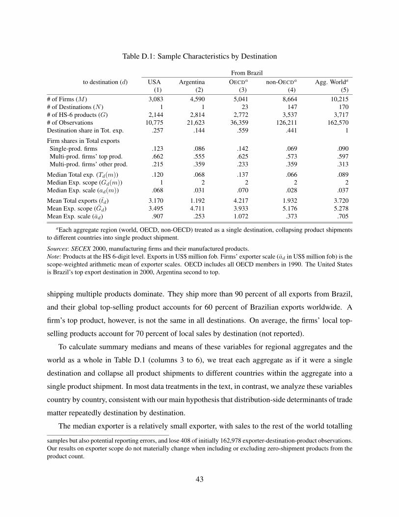
Table D.1: Sample Characteristics by Destination

From Brazilto destination (d) USA Argentina OECDa non-OECDa Agg. Worlda

(1) (2) (3) (4) (5)# of Firms (M ) 3,083 4,590 5,041 8,664 10,215# of Destinations (N ) 1 1 23 147 170# of HS-6 products (G) 2,144 2,814 2,772 3,537 3,717# of Observations 10,775 21,623 36,359 126,211 162,570Destination share in Tot. exp. .257 .144 .559 .441 1

Firm shares in Total exportsSingle-prod. firms .123 .086 .142 .069 .090Multi-prod. firms’ top prod. .662 .555 .625 .573 .597Multi-prod. firms’ other prod. .215 .359 .233 .359 .313

Median Total exp. (Td(m)) .120 .068 .137 .066 .089Median Exp. scope (Gd(m)) 1 2 2 2 2Median Exp. scale (ad(m)) .068 .031 .070 .028 .037

Mean Total exports (td) 3.170 1.192 4.217 1.932 3.720Mean Exp. scope (Gd) 3.495 4.711 3.933 5.176 5.278Mean Exp. scale (ad) .907 .253 1.072 .373 .705

aEach aggregate region (world, OECD, non-OECD) treated as a single destination, collapsing product shipmentsto different countries into single product shipment.

Sources: SECEX 2000, manufacturing firms and their manufactured products.Note: Products at the HS 6-digit level. Exports in US$ million fob. Firms’ exporter scale (ad in US$ million fob) is thescope-weighted arithmetic mean of exporter scales. OECD includes all OECD members in 1990. The United Statesis Brazil’s top export destination in 2000, Argentina second to top.

shipping multiple products dominate. They ship more than 90 percent of all exports from Brazil,

and their global top-selling product accounts for 60 percent of Brazilian exports worldwide. A

firm’s top product, however, is not the same in all destinations. On average, the firms’ local top-

selling products account for 70 percent of local sales by destination (not reported).

To calculate summary medians and means of these variables for regional aggregates and the

world as a whole in Table D.1 (columns 3 to 6), we treat each aggregate as if it were a single

destination and collapse all product shipments to different countries within the aggregate into a

single product shipment. In most data treatments in the text, in contrast, we analyze these variables

country by country, consistent with our main hypothesis that distribution-side determinants of trade

matter repeatedly destination by destination.

The median exporter is a relatively small exporter, with sales to the rest of the world totalling

samples but also potential reporting errors, and lose 408 of initially 162,978 exporter-destination-product observations.Our results on exporter scope do not materially change when including or excluding zero-shipment products from theproduct count.

43

around US$ 89,000. The mean exporter, in contrast, sells around US$ 3.7 million abroad, more

than 40 times as much as the median manufacturer. Exporter scope and exporter scale exhibit sim-

ilarly stark differences between mean and median. The median Brazilian manufacturer sells two

products worldwide, but the mean scope per firm is 5.3 products. The median Brazilian manufac-

turer has a product scale of around US$ 37,000 per product, but the exporter scale per exporter is

US$ 705,000, or around 20 times as high as that for the median firm.40

The importance of the top-selling product at multi-product exporters and the mean-median ra-

tios repeat across destinations. To investigate the robustness across countries, we select Brazil’s

top two export destinations (United States and Argentina), as well as the OECD and non-OECD ag-

gregates. Our theory emphasizes the importance of exporting behavior within destinations. Within

single countries, the mean manufacturer’s exports exceed the median manufacturer’s exports by

similarly large factors as in the aggregate, between 14 (in Argentina, column 2) and 26 (in the

United States, column 1). In the OECD aggregate (column 3), exports of the mean firm exceed the

exports of the median firm by a factor of about 30. Interestingly, the same mean-median ratio of

about 30 prevails in the non-OECD aggregate.

We further investigate the striking similarity of firm scope choices across destinations by relat-

ing the mean number of products to market characteristics. For this purpose, we consider a further

decomposition of the left-hand side variable: define tsd as the mean sales of firms from s selling

to d divided by the exporter scale of these firms in market d. Thus tsd ≡ Gsd tsd/Gsd ≡ Gsd asd,

where Gsd is the exporter mean exporter scope and asd ≡ td/Gsd is the exporter mean product

scale per product. We regress the log mean exporter scope Gd on the log of λsdTsd.

ln Gsd = 2.324(.676)

+ .087(.057)

lnλsd − .058(.046)

lnTsd.

The R2 is .281 (standard errors in parentheses). Neither market share nor market size are statisti-

cally significant predictors of exporter scope at conventional levels.41 So, most of the variation in

firms’ exports to a market is due to variation in their mean scale per product.

At the firm level, the Brazilian data exhibit market-presence patterns broadly similar to the40The means in Table D.1 are calculated as follows. A source country’s total exports Td are decomposed into

Td = Md Gd ad, where Md is the number of exporters to destination d, Gd ≡∑Md

ϕ=1 Gd(ϕ)/Md is the exporters’ meanexporter scope, and ad ≡ td/Gd is their products’ exporter scale. Equivalently, ad is the weighted arithmetic meanof ad(ϕ) over all ϕ, with weights Gd(ϕ): ad =

∑Md

ϕ=1 Gd(ϕ) ad(ϕ)/[∑Md

ϕ=1 Gd(ϕ)] = td/Gd. As the decompositionshows, scope weighting is necessary for the mean scope and the exporter scale to yield total exports when multiplied.

41The R2 drops to .212 when including lnMsd and industry fixed effects but coefficients become statistically sig-nificant at conventional levels except for market size, while magnitudes change little.

44

French and U.S. firm-destination data. Similar to Eaton, Kortum, and Kramarz (2004), for instance,

the elasticity of the number of firms with respect to the number of export destinations is about -2.5,

just as for French exporters.

D.2 Estimation of Figure 1 (Fact 1)

To generate data such as those in Figure 1 (Fact 1), we aggregate individual product sales by

averaging over all products of a given rank and all firms with a given exporter scope in a destination.

As shown in Appendix A.3, our model implies that the regression equation for average product

sales in Figure 1 is

ln asd = ln θσθ−(σ−1)fsd(1) + [δ + α(σ−1)] lnGsd(ϕ)− [α(σ−1)] ln g

+ ln[1− [Gsd/(Gsd+1)](θ−1)(δ+α(σ−1))

]− ln

[1− [Gsd/(Gsd+1)]θ(δ+α(σ−1))

]for g ≤Gsd, where asd ≡

∫ ϕ∗,G+1sd

ϕ∗,Gsd

psdg(ϕ) xsdg(ϕ)[θ/ϕθ+1][1/(ϕ∗,G

sd )−θ − (ϕ∗,G+1sd )−θ] dϕ is average

product sales for a product of rank g over all firms with exporter scope Gsd.

We fit this regression equation with non-linear least squares under three choices of the free pa-

rameter: θ = 1.06 (as used by Luttmer (2007) and di Giovanni and Levchenko (2010) and reported

by Axtell (2001)); θ = 1.28 (our middle-ground benchmark for counterfactual simulations); and

θ = 1.49 (as reported by Arkolakis (2010)). We find for δ + α(σ−1) estimates of 1.60 and 1.61

under the three parametrizations and for α(σ−1) an estimate of 2.55 under all three parametriza-

tions. These estimates closely resemble those in Table 3. Not surprisingly, the estimate for α(σ−1)is close to the slopes between 2.6 and 2.8 that were reported in Section 2.2 for Figure 1.

D.3 Data for simulations

For bilateral trade and trade balances in manufacturing products, we use World Trade Flow (WTF)

data in U.S. dollars for the year 2000 (Feenstra, Lipsey, Deng, Ma, and Mo 2005). To mitigate the

effect of entrepot trade, we follow Dekle, Eaton, and Kortum (2007) and collapse (i) Hong Kong,

Macao and mainland China, (ii) Belgium, Luxembourg and the Netherlands, and (iii) Indonesia,

Malaysia, Singapore, and Thailand into single entities. In 2000, import information for India is

missing from WTF. We obtain information for India in 2000 from UN Comtrade. We keep only

manufactured products from the WTF data, using a concordance from the OECD at the SITC

45

revision-2 4-digit level to determine manufactured products. So our final bilateral trade data set

excludes agricultural and mining commodities. By our construction, the world’s trade balance in

manufactures is zero.

For information on GDP, manufacturing value added and the overall trade balances in goods

and services in 2000 we use the World Bank’s World Development Indicators 2009 (WDI). India

included, our initial WTF sample has 132 countries that can be matched to the WDI data, and

we collapse bilateral trade for the rest of the world by trade partner into a 133rd observation. We

compute GDP and manufacturing value added for the rest of the world as the WDI reported world

total less the sample total of our 132 matched countries. We set the overall trade balances in goods

and services for the rest of the world so that the world total is zero.

We obtain β from the UNIDO Industrial Statistics Database at the 3-digit ISIC level (revi-

sion 2), which offers both manufacturing value added and manufacturing gross production for 51

of our sample countries and the rest of the world. Averaging the ratio of manufacturing value added

to manufacturing output in 2000 over these countries yields β = .330. This worldwide β estimate

enters our computation of γd by (B.9).

We finally need information on manufacturing absorption. Following Eaton, Kortum, and Kra-

marz (2004), we infer manufacturing absorption as manufacturing output (from the UNIDO Indus-

trial Statistics Database 2005) plus the trade deficit (from WTF). The UNIDO data for manufac-

turing output are considerably less complete than either WTF or WDI. We obtain manufacturing

output for Brazil from the Brazilian statistical agency IBGE (2010). Our final country sample for

which we have manufacturing absorption contains 57 countries. By the model in Appendix B, γd

is given as (B.9). We use our WTF-WDI-UNIDO data to calculate γd by country. For the rest of

the world, we set γd to the sample average over our 57 countries (average γ = .244) and back out

manufacturing absorption for the rest of the world from (B.9).

46

ReferencesALLANSON, P., AND C. MONTAGNA (2005): “Multiproduct Firms and Market Structure: An

Explorative Application to the Product Life Cycle,” International Journal of Industrial Organi-zation, 23(7-8), 587–97.

ALVAREZ, F., AND R. E. J. LUCAS (2007): “General Equilibrium Analysis of the EatonKortumModel of International Trade,” Journal of Monetary Economics, 54(6), 1726–68.

ALVAREZ, R., H. FARUQ, AND R. A. LOPEZ (2007): “New Products in Export Markets: Learningfrom Experience and Learning from Others,” Indiana University, Bloomington, unpublishedmanuscript.

ANDERSON, J. E., AND E. VAN WINCOOP (2003): “Gravity with Gravitas: A Solution to theBorder Puzzle,” American Economic Review, 93(1), 170–92.

ARKOLAKIS, C. (2010): “Market Penetration Costs and the New Consumers Margin in Interna-tional Trade,” Journal of Political Economy, forthcoming.

ARKOLAKIS, C., A. COSTINOT, AND A. RODRIGUEZ-CLARE (2009): “New Trade Models,Same Old Gains?,” NBER Working Paper, 15628.

ARKOLAKIS, C., AND M.-A. MUENDLER (2010): “The Extensive Margin of Exporting Products:The Continuum Case,” University of California, San Diego, unpublished manuscript.

ARMENTER, R., AND M. KOREN (2010): “A Balls-and-Bins Model of Trade,” Central EuropeanUniversity, unpublished manuscript.

ATKESON, A., AND A. T. BURSTEIN (2008): “Pricing-to-Market, Trade Costs, and InternationalRelative Prices,” American Economic Review, 98(5), 1998–2031.

(2010): “Innovation, Firm Dynamics, and International Trade,” Journal of Political Econ-omy, 118(3), 433–484.

AXTELL, R. L. (2001): “Zipf Distribution of U.S. Firm Sizes,” Science, 293(5536), 1818–20.

BALDWIN, R. E. (2000): “Regulatory Protectionism, Developing Nations, and a Two-Tier WorldTrade System,” Brookings Trade Forum, 2000(1), 237–280.

BAYUS, B. L., AND J. W. P. PUTSIS (1999): “Product Proliferation: An Empirical Analysis ofProduct Line Determinants and Market Outcomes,” Marketing Science, 18(2), 137153.

BERGSTRAND, J. H., P. EGGER, AND M. LARCH (2010): “Gravity Redux: Estimation of Gravity-Equation Coefficients, Elasticities of Substitution, and General Equilibrium Comparative Staticsunder Asymmetric Bilateral Trade Costs,” University of Notre Dame, unpublished manuscript.

BERNARD, A. B., J. B. JENSEN, AND P. K. SCHOTT (2009): “Importers, Exporters, and Multina-tionals: A Portrait of Firms in the U.S. that Trade Goods,” in Producer Dynamics: New Evidencefrom Micro Data, ed. by T. Dunne, J. B. Jensen, and M. J. Roberts, vol. 68 of Studies in Incomeand Wealth, chap. 14, pp. 513–552. University of Chicago Press, Chicago.

47

BERNARD, A. B., S. J. REDDING, AND P. K. SCHOTT (2010a): “Multi-product Firms and TradeLiberalization,” Quarterly Journal of Economics, forthcoming.

(2010b): “Multiple-Product Firms and Product Switching,” American Economic Review,100(1), 7097.

BRAMBILLA, I. (2009): “Multinationals, Technology, and the Introduction of Varieties of Goods,”Journal of International Economics, 79(1), 89–101.

BRODA, C., AND D. E. WEINSTEIN (2006): “Globalization and the Gains from Variety,” Quar-terly Journal of Economics, 121(2), 541–85.

CHANEY, T. (2008): “Distorted Gravity: The Intensive and Extensive Margins of InternationalTrade,” American Economic Review, 98(4), 1707–21.

CUMMINS, J. D., M. A. WEISS, X. XIE, AND H. ZI (2010): “Economies of Scope in FinancialServices: A DEA Efficiency Analysis of the U.S. Insurance Industry,” Journal of Banking andFinance, 34(7), 1525–1539, Special Issue.

DAS, S., M. J. ROBERTS, AND J. R. TYBOUT (2007): “Market Entry Costs, Producer Hetero-geneity, and Export Dynamics,” Econometrica, 75(3), 837–73.

DEARDORFF, A. V., AND R. M. STERN (1998): Measurement of nontariff barriers, Studies inInternational Economics. University of Michigan Press, Ann Arbor.

DEKLE, R., J. EATON, AND S. KORTUM (2007): “Unbalanced Trade,” American Economic Re-view: Papers and Proceedings, 97(2), 351–55.

DHINGRA, S. (2010): “Trading Away Wide Brands for Cheap Brands,” University of Wisconsin-Madison, unpublished manuscript.

DI GIOVANNI, J., AND A. A. LEVCHENKO (2010): “Firm Entry, Trade, and Welfare in Zipf’sWorld,” University of Michigan, unpublished manuscript.

EATON, J., AND S. KORTUM (2002): “Technology, Geography, and Trade,” Econometrica, 70(5),1741–79.

EATON, J., S. KORTUM, AND F. KRAMARZ (2004): “Dissecting Trade: Firms, Industries, andExport Destinations,” American Economic Review: Papers and Proceedings, 94(2), 150–54.

(2010): “An Anatomy of International Trade: Evidence from French Firms,” Universityof Chicago, unpublished manuscript.

ECKEL, C., L. IACOVONE, B. JAVORCIK, AND J. P. NEARY (2010): “Multi-product Firms atHome and Away: Cost- versus Quality-based Competence,” University of Oxford, unpublishedmanuscript.

ECKEL, C., AND J. P. NEARY (2010): “Multi-Product Firms and Flexible Manufacturing in theGlobal Economy,” Review of Economic Studies, 77(1), 188–217.

48

FEENSTRA, R. C., R. E. LIPSEY, H. DENG, A. C. MA, AND H. MO (2005): “World Trade Flows:1962-2000,” NBER Working Paper, 11040.

FEENSTRA, R. C., AND H. MA (2008): “Optimal Choice of Product Scope for MultiproductFirms under Monopolistic Competition,” in The Organization of Firms in a Global Economy,ed. by E. Helpman, D. Marin, and T. Verdier, chap. 6, pp. 173–199. Harvard University Press,Cambridge, Mass.

GOLDBERG, P., A. KHANDELWAL, N. PAVCNIK, AND P. TOPALOVA (2010): “Imported Inter-mediate Inputs and Domestic Product Growth: Evidence from India,” Quartery Journal of Eco-nomics, forthcoming.

HELPMAN, E., M. MELITZ, AND Y. RUBINSTEIN (2008): “Estimating Trade Flows: TradingPartners and Trading Volumes,” Quarterly Journal of Economics, 123(2), 441–87.

HELPMAN, E., M. J. MELITZ, AND S. R. YEAPLE (2004): “Export versus FDI with Heteroge-neous Firms,” American Economic Review, 94(1), 300–316.

IACOVONE, L., AND B. S. JAVORCIK (2008): “Shipping Good Tequila Out: Investment, Domes-tic Unit Values and Entry of Multi-product Plants into Export Markets,” University of Oxford,unpublished manuscript.

LUTTMER, E. G. J. (2007): “Selection, Growth, and the Size Distribution of Firms,” QuarterlyJournal of Economics, 122(3), 1103–44.

MASKUS, K. E., T. OTSUKI, AND J. S. WILSON (2005): “The Cost of Compliance with Prod-uct Standards for Firms in Developing Countries: an Econometric Study,” World Bank PolicyResearch Working Paper, 3590.

MASKUS, K. E., AND J. S. WILSON (eds.) (2001): Quantifying the Impact of Technical Barriersto Trade: Can It Be Done?, Studies in International Economics. University of Michigan Press,Ann Arbor, Michigan.

MAYER, T., M. J. MELITZ, AND G. I. P. OTTAVIANO (2009): “Market size, Competition, andthe Product Mix of Exporters,” Harvard University, unpublished manuscript.

MELITZ, M. J. (2003): “The Impact of Trade on Intra-Industry Reallocations and AggregateIndustry Productivity,” Econometrica, 71(6), 1695–1725.

MORGAN, N. A., AND L. L. REGO (2009): “Brand Portfolio Strategy and Firm Performance,”Journal of Marketing, 73(1), 59–74.

NOCKE, V., AND S. R. YEAPLE (2006): “Globalization and Endogenous Firm Scope,” NBERWorking Paper, 12322.

PANZAR, J. C., AND R. D. WILLIG (1977): “Economies of Scale in Multi-Output Production,”Quarterly Journal of Economics, 91(3), 481–493.

(1981): “Economies of Scope,” American Economic Review, 71(2), 268–272.

49

RUDIN, W. (1976): Principles of Mathematical Analysis. McGraw and Hill, New York, New York,3rd edn.

THOMAS, C. (2010): “Too Many Products: Decentralized Decision-Making in MultinationalFirms,” Columbia Business School, unpublished manuscript.

WORLD BANK (2003): Global Economic Prospects 2004: Realizing the Development Promise ofthe Doha Agenda. World Bank, Washington, DC.

WTO (2008): World Trade Report: Trade in a Globalizing World. World Trade Organization,Geneva.

50