NBER WORKING PAPER SERIES

LIQUIDITY AND THE THREAT OF FRAUDULENT ASSETS

Yiting LiGuillaume RocheteauPierre-Olivier Weill

Working Paper 17500http://www.nber.org/papers/w17500

NATIONAL BUREAU OF ECONOMIC RESEARCH1050 Massachusetts Avenue

Cambridge, MA 02138October 2011

A previous version of this paper was circulated under the title "Liquidity Constraints." We thank twoanonymous referees and Rob Shimer for comments that greatly improved the paper. We also thankVeronica Guerrieri for an insightful discussion, Andy Atkeson, Bill Branch, Dean Corbae, HaroldDemsetz, Manolis Galenianos, Hugo Hopenhayn, Thomas Philippon, Shouyong Shi, and seminar participantsat the Bank of Canada, the Federal Reserve Bank of Chicago, the Federal Reserve Bank of Cleveland,the National University of Seoul, the National Taiwan University, the Singapore Management University,the University of California at Riverside and Santa Cruz, the University of Wisconsin, and the Whartonschool at the University of Pennsylvania for useful comments. We thank Monica Crabtree-Reusserfor editorial assistance. The views expressed herein are those of the authors and do not necessarilyreflect the views of the National Bureau of Economic Research.

NBER working papers are circulated for discussion and comment purposes. They have not been peer-reviewed or been subject to the review by the NBER Board of Directors that accompanies officialNBER publications.

© 2011 by Yiting Li, Guillaume Rocheteau, and Pierre-Olivier Weill. All rights reserved. Short sectionsof text, not to exceed two paragraphs, may be quoted without explicit permission provided that fullcredit, including © notice, is given to the source.

Liquidity and the Threat of Fraudulent AssetsYiting Li, Guillaume Rocheteau, and Pierre-Olivier WeillNBER Working Paper No. 17500October 2011JEL No. E41,E44,E5,E58,G1,G12

ABSTRACT

We study an over-the-counter (OTC) market with bilateral meetings and bargaining where the usefulnessof assets, as means of payment or collateral, is limited by the threat of fraudulent practices. We assumethat agents can produce fraudulent assets at a positive cost, which generates endogenous upper boundson the quantity of each asset that can be sold, or posted as collateral in the OTC market. Each endogenous,asset-specific, resalability constraint depends on the vulnerability of the asset to fraud, on the frequencyof trade, and on the current and future prices of the asset. In equilibrium, the set of assets can be partitionedinto three liquidity tiers, which differ in their resalability, their prices, their sensitivity to shocks, andtheir responses to policy interventions. The dependence of an asset's resalability on its price createsa pecuniary externality, which leads to the result that some policies commonly thought to improveliquidity can be welfare reducing.

Yiting LiDepartment of EconomicsNational Taiwan University21 Hsu-Chow Rd. 100 Taipei, Taiwanyitingli@ntu.edu.tw

Guillaume RocheteauDepartment of EconomicsUniversity of California at Irvine3151 Social Science PlazaIrvine, California 9269grochete@uci.edu

Pierre-Olivier WeillDepartment of EconomicsUniversity of California, Los AngelesBunche Hall 8283Los Angeles, CA 90095and NBERpoweill@econ.ucla.edu

1 Introduction

Liquidity premia, or convenience yields, are key determinants of asset prices. This point is un-

controversial for fiat money, which derives its value solely from its liquidity services. According

to Krishnamurthy and Vissing-Jorgensen (2010), the same is true for government securities, high-

grade corporate bonds, and agency bonds. In this paper we present a theory of asset liquidity and

convenience yields, based on the following premise: an asset’s liquidity—the extent to which it can

facilitate exchange, as means of payment or as collateral—depends on its vulnerability to fraud. We

address a class of questions related to the cross-sectional dispersion and time-variation of liquidity

premia, such as what fundamental characteristics make some assets have higher turnover and lower

yields than others? What shocks prompt investors to suddenly shift their portfolios towards the

most liquid assets, which leads to widening yield spreads? Are liquid assets more susceptible of

exhibiting excess volatility? And, what types of open-market operations and financial regulations

are effective to mitigate aggregate liquidity shortages?

The threat of fraud has been a pervasive friction throughout history. Classical examples include

the clipping of coins in ancient Rome and medieval Europe, and the counterfeiting of banknotes

during the first half of the 19th century in the United States (Sargent and Velde, 2002; Mihm,

2007). Modern financial assets are no less susceptible to fraud. Intangible means of payment suffer

from identity thefts (Schreft, 2007), and mortgage-backed securities are subject to moral hazard

problems and lax incentives that plague the process of securitization (see, among others, Keys,

Mukherjee, Seru, and Vig, 2010).1 Similarly, the fact that some investors can spend resources to

cherry-pick the collateral used to secure risk-sharing arrangements is a concern for participants in

OTC derivative markets.2

We introduce the threat of fraud into a search-theoretic model of asset markets, building on

1The 2010 “Performance and Activity Report” of the SEC details many cases of financial fraud related tomortgage-based securities. Frauds and moral hazard problems in the mortgage market are not new. Snowden(2010) describes the US mortgage crisis of the late 20s and 30s and the earlier forms of securitization in the 20s. Realestate bond houses were overappraising properties, they violated underwriting standards, and they substituted badloans for performing mortgages in their mortgage pools.

2The International Swap and Derivatives Association (2010) reported that over 78% of OTC derivatives tradesare collateralized. Importantly, market participants consider some asset classes (e.g., cash or government securities)to be of higher collateral quality than others. Collateral quality depends on various factors such as volatility, creditrisk, and pricing ease.

1

recent work in monetary and financial economics (e.g., Lagos and Wright, 2005; Duffie, Garleanu,

and Pedersen, 2005). In the first period, agents trade an arbitrary number of assets in a competitive

market. In the second period, they trade goods and services in an over-the-counter (OTC) market,

with bilateral meetings and bargaining. Because of the frictions caused by a lack of commitment

and limited enforcement, agents use assets as means of payment, or as collateral, in the OTC

market. However, the extent to which an asset can play such a role is limited by the threat of

fraud: after incurring an asset-specific fixed cost, an agent can produce fraudulent assets, which

are worthless and indistinguishable from their genuine counterparts. In order to solve the resulting

OTC bargaining problem under asymmetric information, we assume that the asset holder makes a

take-it-or-leave-it offer, and we use the recent methodology of In and Wright (2011) for signaling

games with hidden choices to select an equilibrium.

A key insight of our analysis is that the threat of fraud generates asset-specific, endogenous

resalability constraints. While there are no exogenous restrictions on the transfer of assets in

bilateral matches in the OTC market, if the quantity of an asset offered is above some threshold,

then the trade is rejected with positive probability because of the rational fear that the asset might

be fraudulent. In equilibrium, agents never find it optimal to offer more of the asset than what

can be accepted with certainty, which prevents fraud from taking place. The resulting endogenous

resalability constraint has three determinants: the asset’s vulnerability to fraud, the difference

between the asset’s price and the discounted value of its cash flows, and the frequency of trades in

OTC markets. We emphasize three main implications of these endogenous resalability constraints

below.

First, because an asset’s resalability depends on its own vulnerability to fraud, prices and mea-

sures of liquidity vary across assets with identical cash flows. We obtain an endogenous three-tier

categorization of assets: illiquid, partially liquid, and liquid assets, which differ in their resalability,

their price, as well as their sensitivity to shocks and policy interventions. While the price of an

illiquid asset is equal to the present value of its cash flows, the price of a partially liquid or liquid

asset is strictly larger than the present value of its cash flows; i.e., this asset enjoys a liquidity

premium. This premium increases with the asset’s recognizability but decreases with its supply,

which is consistent with the downward-sloping aggregate demand for Treasury debt documented

2

in Krishnamurthy and Vissing-Jorgensen (2010). Finally, while the prices of illiquid and partially

liquid assets are constant in the absence of shocks to fundamentals, the prices of liquid assets can

exhibit self-fulfilling fluctuations.

Second, in a similar spirit as Guerrieri and Shimer (2011), our model identifies shocks that

generate phenomena akin to flights to liquidity, whereby investors shift their asset demands from

less liquid to more liquid assets, widening the liquidity spread between the two types of assets

(see Longstaff, 2004, and Dick-Nielsen, Feldhutter, and Lando, 2010). For instance, we consider

an increase in the frequency of liquidity needs in the OTC market that results in higher demand

for collateral. Such a shock increases the value of holding assets, as they are more likely to be

used as means of payment or as collateral, but it also has the countervailing effect of increasing

fraud incentives. We show that the first effect dominates for liquid assets and raises their prices,

while the second effect dominates for partially liquid assets and lowers their prices. Moreover,

the set of liquid assets endogenously shrinks, meaning that agents shift their demand to the most

recognizable assets, in accordance with a flight to liquidity. The same phenomenon can be generated

in our model by a shock that raises the threat of fraud for some partially liquid or liquid assets,

thereby reducing their resalability.

The third main implication of our results concerns policies aimed at managing the aggregate

supply of liquidity through open-market operations or financial regulations. In our model, an

open-market operation has a positive welfare effect if and only if it increases a simple measure of

aggregate liquidity—a weighted sum of asset supplies. Therefore, a substitution of liquid assets with

other liquid assets is irrelevant. An open-market purchase of illiquid assets with liquid ones, on the

other hand, raises aggregate liquidity and output. However, under a balanced budget requirement,

a purchase of partially liquid assets with liquid ones reduces aggregate liquidity, the yield of liquid

assets, and output. This paradoxical result arises because of a ”pecuniary externality,” according to

which an increase in the price of an asset reduces its resalability, which in turn can lower its liquidity

premium below the true marginal social value of its liquidity services. Due to this externality, a

balanced budget open-market purchase syphons out more liquidity than it is injecting in. This

result can shed some light on quantitative easing, which consists of injecting reserves in exchange

for less liquid assets (Krishnamurthy and Vissing-Jorgensen, 2011). According to our model, for

3

such policies to successfully increase aggregate liquidity, they must target the most illiquid assets.

In a similar vein, we study retention requirements that were introduced by the Dodd-Frank Act to

mitigate moral hazard problems in the securitization process. In the context of our model, such

requirements are welfare improving only if applied to illiquid assets.

1.1 Literature review

Kiyotaki and Moore (2001, 2005) study limited resalability by assuming that each period, agents

cannot sell more than an exogenous proportion of their asset holdings. While such exogenous

resalability constraints can be chosen to replicate our distribution of asset prices, they generate

markedly different comparative statics and policy recommendations (see Supplementary Appendix

E). For instance, with proportional resalability constraints, an increase in the frequency of trading

needs weakly increases the prices of all assets, while in our model it has asymmetric effects: it

increases the prices of liquid assets, and decreases the prices of partially liquid assets, consistent

with evidence on flight to liquidity. As another example, with proportional liquidity constraints,

an open-market purchase of partially liquid assets with liquid ones increases liquidity, asset yields,

and welfare. In our model, because of a new pecuniary externality, we obtain the opposite effects,

consistent with evidence on quantitative easing.

In Holmstrom and Tirole’s (2011, and references therein) corporate finance model, a moral

hazard problem generates endogenous borrowing constraints, i.e., resalability constraints in the

primary asset market. In the secondary market, corporate claims with identical cash flows enjoy the

same liquidity premium. In our model, by contrast, we focus on moral hazard in secondary markets.

We highlight the fact that agents’ incentives to take hidden actions depend on contemporaneous

secondary market prices and on OTC market frictions, and we generate cross-sectional differences

in liquidity premia between assets with identical cash flows.

The search-theoretic literature on the liquidity structure of asset returns includes, e.g., Wallace

(1998, 2000), Weill (2008), and Lagos (2010), and related work on the rate-of-return-dominance

puzzle. Our approach goes beyond this earlier search literature by showing how cross-sectional

differences in liquidity arise from fraud-based endogenous resalability constraints.3 Lester, Postle-

3Wallace (1998, 2000) emphasizes assets’ indivisibilities, Weill (2008) assumes increasing returns in the matching

4

waite, and Wright (2011) consider a private information problem where agents can recognize the

quality of an asset at some cost, but to determine the terms of trade under asymmetric informa-

tion they make the simplifying assumption that unrecognized assets are not accepted in a bilateral

match.4 They address this issue in an extension that follows our methodology closely.

There is a literature that emphasizes adverse selection problems in asset markets with search

frictions (e.g., Hopenhayn andWerner, 1996). The most closely related papers are Rocheteau (2009)

who introduces an adverse selection problem in a monetary model to explain the illiquidity of risky

assets, and Guerrieri, Shimer, and Wright (2010), who consider a competitive search environment to

illustrate how trading delays emerge endogenously to screen high- and low-quality assets. Guerrieri

and Shimer (2011) extend the previous paper to a general equilibrium framework and, among

other results, provide an explanation for flights to liquidity based on a dynamic adverse selection

problem. While the distinction between adverse selection and moral hazard in asset markets is

often subtle, the methodologies for capturing the two frictions differ profoundly. We take the

view that informational asymmetries in asset markets often result from strategic behavior, which

allows us to focus the model more squarely on the effects of the threat of fraud on asset liquidity.

At a more theoretical level, an important distinction between adverse selection and moral hazard

is that the type distribution is exogenous with the former, but is endogenous with the latter.

With an exogenous type distribution, under some conditions, agents can mitigate the asymmetric

information friction by holding broadly diversified asset portfolios. As our model demonstrates,

when the type distribution is endogenous, the asymmetric information friction remains relevant.

The next section presents the model. Section 3 solves the bargaining game under the threat

of fraud. Section 4 solves for asset prices, and Section 5 presents three main implications. The

appendix contains omitted proofs, and the supplementary appendix presents additional results and

extensions.

technology, and Lagos (2010) introduces exogenous restrictions on the use of some assets as means of payment.Similarly, Shi (2008) studies the pricing of bonds in a search economy where exogenous legal restrictions preventbonds from being used in payments in a fraction of trades.

4There is also a related literature on counterfeiting, e.g., Green and Weber (1996), Williamson and Wright (1994),and Nosal and Wallace (2007). In those studies, there is a single asset, asset holdings are restricted to {0, 1}, andassets are indivisible, while those restrictions are all relaxed in our model.

5

CM DM

competitive market

decision to producefraudulent assets

decentralized market:bilateral matchesand bargaining

Figure 1: Timing of the game.

2 The model

The economy lasts for two periods, t ∈ {0, 1}, and is populated by a continuum of agents who

trade sequentially in two markets: in a centralized market (CM) at t = 0, and in a decentralized

over-the-counter market (DM) at t = 1. There are two perfectly divisible and perishable goods.

The first good, which we take to be the numeraire, is produced and consumed at t = 0 and at

the end of t = 1. The second good, labeled the DM good, is produced and consumed in bilateral

meetings in the DM. There is a finite set of assets indexed by s ∈ S. Each asset pays off at the end

of t = 1 a dividend normalized to one unit of the numeraire.

Agents are divided evenly into two types, called buyers and sellers. Buyers wish to consume in

the DM but cannot produce, while sellers have the technology to produce goods in the DM but do

not want to consume. Together with frictions described below, this preference structure creates a

need for liquidity: buyers will acquire assets in the CM in order to finance the purchase of goods

produced by sellers in the DM. The utility of a buyer is:

x0 + β [u(q1) + x1] , (1)

where xt ∈ R is the consumption of the numeraire good at time t, with xt < 0 being interpreted

as production, q1 ∈ R+ is the consumption of the DM good, and β ≡ (1 + r)−1 ∈ (0, 1) is a

discount factor. The utility function, u(q), over the DM good is twice continuously differentiable,

with u(0) = 0, u�(q) > 0, u�(0) = ∞, u�(∞) = 0, and u��(q) < 0. The utility of a seller is:

x0 + β (−q1 + x1) , (2)

where q1 is the seller’s production in a pairwise meeting in the DM. Let q∗ = argmaxq [u(q)− q] > 0

denote the output level that maximizes the match surplus, so u�(q∗) = 1.

6

The CM is a perfectly competitive market, where agents trade the numeraire good and assets.

The DM, on the other hand, is an over-the-counter market, where a fraction σ ∈ (0, 1] of buyers

are matched bilaterally and at random with an equal fraction of sellers. Because of a lack of

commitment and limited enforcement, buyers purchase DM goods with assets or, equivalently, with

loans collateralized by assets (see footnote 11).

Terms of trade in pairwise meetings in the DM are determined according to a simple bargaining

game, in which the buyer makes a take-or-leave-it offer.5 The buyer, whose asset holdings are private

information, asks for a given amount of the DM good in exchange for some specified portfolio of

assets.6 The seller accepts or rejects the offer. If the seller accepts the offer, then the trade is

implemented, provided that the asset transfer is feasible given the buyer’s asset holdings. Matched

agents split apart before assets pay off.

We introduce the possibility of asset fraud as follows. In the CM at t = 0, a buyer can pay a

fixed cost k(s) > 0 to produce any quantity of fraudulent asset of type s. Fraudulent assets have

zero terminal value and, in the DM, cannot be distinguished by sellers from genuine assets.

2.1 Interpretations

Counterfeiting of a means of payment. A literal interpretation of the model concerns assets

used as means of payment, such as coins or banknotes, for which the fraud consists of producing

counterfeits.7 During the first half of the 19th century, the fixed cost to produce fake banknotes in-

cluded the cost to acquire plates and dies. See, e.g., Mihm (2007). Nowadays, this cost corresponds

to the price of photo-editing software and copy machines.

5In her discussion of our paper, Veronica Guerrieri investigated a version of the model with competitive searchand showed that this alternative pricing mechanism generates the same liquidity constraint as the one obtained underour simple bargaining game.

6By assuming that asset holdings are unobservable, we reduce the set of signals sent by a buyer, which simplifiesthe analysis. As shown in the earlier version of our working paper, results are robust to alternative assumptionsregarding the observability of asset holdings. Also, we do not allow buyers to offer lotteries over allocations. Inour context we conjecture that it is with no loss in generality, but such lotteries could be useful in the presence ofalternative cost structures of producing fraudulent assets—see Supplementary Appendix C on variable costs.

7Our model can accommodate fraud on unsecured credit in bilateral matches. In this case, an agent has theoption to produce a fake identity in the CM at a fixed cost (e.g., the cost incurred by a computer hacker to steal theidentity of someone else) and he can issue an IOU in the DM if matched. The repayment of genuine IOUs can beenforced in the following CM. In contrast, IOUs based on fake identities are not repaid.

7

Collateral fraud. An alternative interpretation is that buyers use assets as collateral to secure

loans to be repaid at the end of t = 1. If the asset is a house, the transaction in the DM is an equity

extraction loan to finance consumption. An example of mortgage fraud that closely resembles our

model is the property flipping scheme, whereby a buyer obtains a high-loan-to-value mortgage

based on a fake property appraisal, and the bank is left with worthless collateral.8 In this example,

the cost of producing fraudulent assets represents the cost of creating false documentation about

the borrower and the property. The DM can also be interpreted as an OTC market for credit

derivatives, such as the market for credit default swaps or interest rate swaps. In that context, the

goods traded in the DM are risk-sharing services, and collateral is used to mitigate counterparty

risk.9 The cost of producing fraudulent assets is the informational cost incurred by the buyer to

identify bad collateral. This cost is related to the complexity of the asset, its issuer, and the quality

and quantity of information released about the asset’s cash flows.

Securitization fraud. In this context buyers represent mortgage securitizers who originate and

package loans in the CM. Sellers represent final asset holders who acquire securitized assets in

the DM. There are gains from trading assets in the DM because it allows mortgage securitizers

to spread the risk of the underlying loans to final asset holders.10 In this example, the cost of

producing fraudulent assets is the cost of generating false documentation about the underlying

security, bribing an agency for a good rating, or engaging in accounting frauds.

3 Bargaining under the threat of fraud

In this section we solve for the equilibrium of the game between a buyer and a seller matched at

random. The game starts in the CM at t = 0 and ends in the DM at t = 1. For now we take as

given asset prices in the CM, φ(s), s ∈ S, and we anticipate that, in equilibrium, they will satisfy

8See http://www.fbi.gov/about-us/investigate/white collar/mortgage-fraud/mortgage fraud.9In Supplementary Appendix G, we provide an explicit model of risk-sharing arrangements, where the DM good

can be interpreted as risk-sharing services.10In Supplementary Appendix H, we provide such a model of securitization, where agents have Constant Absolute

Risk Aversion (CARA) utilities. This model confirms, albeit with different functional forms, that u(q) can beinterpreted as the utility of reducing the securitizer’s risk position, and q = c(q) can be interpreted as the cost ofincreasing the final asset holder’s risk position.

8

φ(s) ≥ β; i.e., the rate of return of asset s is no greater than the discount rate, which would be the

“fundamental price” of the asset in a frictionless economy.

The sequence of moves is as follows: (i) In the CM at t = 0, the buyer chooses a portfolio of

{a(s)} genuine and {a(s)} fraudulent assets, subject to a(s) ≥ 0 and a(s) ≥ 0; (ii) In the DM

at t = 1, the buyer is matched with a seller with probability σ, in which case he makes an offer

(q, {d(s)}), where q represents the output produced by the seller and d(s) is the transfer of assets

of type s (genuine or fraudulent) from the buyer to the seller; (iii) The seller decides whether to

accept the offer; (iv) If the offer is accepted, the seller delivers q units of goods to the buyer, and

the buyer delivers τ(s) ∈ [0, a(s)] genuine and τ(s) ∈ [0, a(s)] fraudulent units of asset s to the

seller, with τ(s) + τ(s) = d(s).11

Payoffs. The Bernoulli payoff of the buyer is:

−�

s∈S

�k(s)I{a(s)>0} + φ(s)a(s)

�+ βµ

�u(q) +

�

s∈S[a(s)− τ(s)]

�+ β(1− µ)

�

s∈Sa(s),

where I{a(s)>0} = 1 if the buyer produces fraudulent assets of type s, a(s) > 0, and zero otherwise.

In the above, µ = 1 if the buyer meets a seller who accepts his offer, and µ = 0 otherwise. The first

term is the payoff of the buyer at t = 0. In order to accumulate a(s) > 0 fraudulent units of asset

s, the buyer must incur the fixed cost k(s). In order to accumulate a(s) units of genuine asset s, he

must produce φ(s)a(s) units of the numeraire good in the CM. The second term is the discounted

payoff at t = 1 if µ = 1; i.e., if the buyer meets a seller in the DM and his offer is accepted. He

then enjoys the utility of DM good consumption, u(q), as well as the payoff from his net holding

of genuine assets, a(s) − τ(s), the initial amount purchased net of the asset transfer to the seller,

keeping in mind that each unit of genuine asset pays off one unit of the numeraire good at the end

of t = 1. The last term is, similarly, the discounted payoff of the buyer at t = 1 if µ = 0. Collecting

11We can reinterpret the payment, (q, {d(s)}), as a fully collateralized loan, where the buyer promises to repay�s∈S d(s) units of the CM output at the end of period 1. In order to secure the repayment of the loan, the buyer

posts d(s) units of asset s as collateral with a third party. If one asset is fraudulent, then the buyer will choose todefault on his obligation, in which case the seller seizes the assets that serve as collateral. If all assets are genuine,then the buyer is indifferent between repaying his debt or defaulting.

9

terms, we can rewrite the payoff as

−�

s∈S

�k(s)I{a(s)>0} +

�φ(s)− β

�a(s)

�+ βµ

�u(q)−

�

s∈Sτ(s)

�. (3)

Similarly, the Bernoulli payoff of the seller is

βµ

�−q +

�

s∈Sτ(s)

�, (4)

where we anticipate that, in equilibrium, sellers will not find it optimal to accumulate assets in the

CM.12 If the seller accepts the offer (µ = 1), he suffers the disutility of producing, q, and receives

τ(s) genuine units of asset s.

Equilibrium concept. Our equilibrium concept is Perfect Bayesian Equilibrium: actions are

sequentially rational following every history, and beliefs accord with Bayes’s rule whenever it is

possible. The notion of Perfect Bayesian Equilibrium imposes little discipline on the seller’s belief

in the DM regarding the decision of the buyer in the initial stage of the game to produce fraudulent

assets, conditional on an off-equilibrium offer being made. Our approach to circumvent this diffi-

culty consists of adopting a notion of strategic stability, according to which any equilibrium of the

original game should also be an equilibrium of the reverse-ordered game, with the following timing:

(i) The buyer determines his DM offer, (q, {d(s)}), before making any decision in the CM (e.g.,

one interpretation is that he posts an offer at the beginning of the CM for the next DM); (ii) He

chooses his portfolio composed of genuine and fraudulent assets; (iii) He is matched with a seller

who chooses whether to accept or reject the offer.13 This reordered game captures the idea that

12Sellers have no strict incentives to accumulate assets if φ(s) ≥ β, because their asset holdings are not observableand hence do not affect the terms of trade offered by the buyer.

13The re-ordering methodology, called the reordering invariance refinement, was developed by In and Wright(2011) for signaling games with unobservable choices. This refinement is based on the invariance condition of strategicstability from Kohlberg and Mertens (1986), which requires that the solution of a game should also be the solutionof any game with the same reduced normal form. (The intuitive criterion does not apply to our game becausein contrast to standard signaling games types are endogenous.) Beside being powerful in selecting equilibria andtractable (because subgame perfection becomes sufficient to solve the game), this equilibrium notion has a strongdecision-theoretic justification and nice normative properties. Specifically, in our model the reordered game capturesthe idea that upon seeing the buyer’s offer, the seller will infer that the buyer’s unobservable actions (portfolio andproduction of fraudulent assets) were chosen optimally with the offer in mind. (This forward induction logic isreminiscent to the one of most refinements in the signaling literature.) From a normative viewpoint, this refinementhas the appealing property of selecting an equilibrium of the original game that yields the highest payoff to the buyer,the agent making the offer. A more detailed description of the merits of this approach is provided in In and Wright(2011).

10

upon seeing the buyer’s offer, the seller will infer that the buyer’s unobservable actions (portfolio

and production of fraudulent assets) were chosen optimally with the offer in mind. The refinement

is intuitive in that it selects an equilibrium of the original game that yields the highest payoff to

the player making the offer, in our case the buyer. Moreover, it improves tractability as subgame

perfection becomes sufficient to solve the game.

Solving for equilibrium. The analysis of the game can be simplified by making two observations.

First, because of the fixed cost, the buyer will either produce the quantity of fraudulent assets that is

necessary to execute the offer in a match or he will produce no fraudulent asset at all. Consequently,

τ(s) = [1− χ(s)] d(s) and τ(s) = χ(s)d(s), where χ(s) = 0 if the buyer produces fraudulent assets,

and χ(s) = 1 otherwise. Moreover, the buyer must be able to cover his intended transfer of genuine

assets; i.e., a(s) ≥ χ(s)d(s).

Second, we can solve for the buyer’s optimal asset demand before solving for equilibrium offers.

Indeed, if φ(s) = β, it follows from the buyer’s payoff, (3), that any demand satisfying the constraint

a(s) ≥ χ(s)d(s) is optimal. If φ(s) > β, it is costly to hold assets, and so it is optimal to demand

a(s) = χ(s)d(s). In both cases, substituting the optimal asset demands into the objective amounts

to replacing a(s) with χ(s)d(s).

With these observations in mind, a buyer’s strategy specifies the following two objects: the

offer, (q, {d(s)}), and conditional on any offer, a probability distribution over {χ(s)} ∈ {0, 1}S ,

denoted by η. The seller’s strategy specifies, conditional on any offer (q, {d(s)}), the probability of

accepting, denoted by π.

The game is solved by backward induction. Following an offer, (q, {d(s)}), the seller’s decision

to accept a trade must be optimal given the buyer’s decision to produce fraudulent assets; i.e.,

π ∈ arg maxπ∈[0,1]

π

�− q +

�

s∈Sη(s)d(s)

�, (5)

where η(s) denotes the marginal probability of bringing genuine assets of type s.14 The seller’s

value of accepting the offer depends on the disutility of producing q units of goods and on the

14Note that, after replacing a(s) and τ(s) with χ(s)d(s) in (3) and (4), the payoffs of buyers and sellers becomelinear functions of the binary actions {χ(s)}. Therefore, taking expectations with respect to η amounts to replacingχ(s) with the marginal probability η(s).

11

expected quality of the asset transfer, determined by η.

Similarly, following an offer (q, {d(s)}), the buyer’s decision to bring genuine or fraudulent assets

is optimal given the seller’s probability of accepting; i.e.,

{η(s)} ∈ arg max{η(s)}

−�

s∈S

�k(s) [1− η(s)] + [φ(s)− β] η(s)d(s) + βσπη(s)d(s)

�, (6)

where the expression that is maximized consists of the terms in the buyer’s payoff that depend on

η. It shows that there are two gains from producing fraudulent assets: the savings in the holding

cost, φ(s)− β, and the savings in the expected cost of transferring genuine assets to a seller.

Finally, given equilibrium decision rules {η(s)} and π, the optimal offer, (q, {d(s)}), maximizes

the following objective

−�

s∈S

�k(s) [1− η(s)] + [φ(s)− β] η(s)d(s)

�+ βσπ

�u(q)−

�

s∈Sη(s)d(s)

�. (7)

A perfect Bayesian equilibrium that satisfies the reordering invariance refinement is a pair of buyer’s

and seller’s strategies satisfying (5), (6), and (7). The next proposition provides a simple joint

characterization of the asset demands and the offers made in any equilibrium.

Proposition 1 The asset demands, {a(s)}, and the equilibrium offers, (q, {d(s)}), solve:

maxq,{a(s),d(s)}

�−�

s∈S[φ(s)− β] a(s) + βσ [u(q)− q]

�(8)

s.t.

�

s∈Sd(s)− q = 0 (9)

d(s) ≤ k(s)

φ(s)− β + βσ, for all s ∈ S (10)

d(s) ∈ [0, a(s)] , for all s ∈ S. (11)

Moreover, following any equilibrium offer, the buyer transfers genuine assets with probability one,

η(s) = 1 for all s, and the seller accepts the offer with probability one, π = 1.

Proposition 1 shows that equilibrium asset demands and offers maximize the buyer’s expected

utility subject to three constraints. First is the individual rationality constraint, (9), which states

that the seller must be indifferent between accepting and rejecting the offer, given that the buyer’s

12

assets are genuine. The seller’s expected payoff is zero since the bargaining protocol specifies that

the buyer makes a take-it-or-leave-it offer. Second is the incentive compatibility constraint, (10),

which states that the buyer must find it optimal to accumulate genuine assets with probability one,

given that the seller accepts with probability one. Third is the feasibility constraint, (11), which

states that the buyer must hold enough genuine assets to cover his transfer to the seller.

To understand why the buyer finds it optimal to bring genuine assets with probability one,

consider a candidate equilibrium in which he brings genuine assets of type s0 with a probability

η(s0) ∈ (0, 1).15 In this candidate equilibrium, the buyer’s payment capacity is slack. To see this,

notice that the buyer could deviate and demand higher consumption in the DM, q� > q, keep the

same {d(s)}, and compensate the seller by bringing genuine assets of type s0 with higher probability,

η�(s0) > η(s0). This deviation would not change the buyer’s expected cost of transferring assets,

since he is indifferent between genuine or fraudulent assets of type s0. Moreover, by (6), indifference

implies:

k(s0) = [φ(s)− β + βσπ] d(s0) =⇒ π =k(s0)− [φ(s0)− β] d(s0)

βσd(s0);

i.e., the seller’s probability of acceptance, π, is pinned down by the transfer d(s0), and is unaffected

by the increase in q. Taken together, these observations mean that the buyer could increase his

payoff by raising his offer q without changing his expected cost of transferring the asset, and without

changing the seller’s acceptance probability.

Lastly, the proposition shows that, in equilibrium, the buyer always finds it optimal to make an

offer that is accepted with probability one. This result is not obvious because offering more assets

than the threshold of equation (10) has two effects going in opposite directions. The positive effect

is that the buyer can demand a higher q in exchange for a higher d. The negative effect is that

a larger offer increases fraud incentives, and hence it has a positive probability of being rejected.

Our proof shows that, with the fixed cost of producing fraudulent assets, the negative effect always

dominates.16

15Looking at η(s0) > 0 is without loss. See the proof of Proposition 1 for details.16In Supplementary Appendix C, we show that the negative effect also dominates if we add proportional costs of

producing fraudulent assets provided that those costs are not too large. If the proportional costs are large relativeto the fixed costs, then there can be situations where fraud generates rationing both at the intensive margin (thequantity of assets that can be transferred in a match) and at the extensive margin (the number of matches in whichtrade occurs).

13

Endogenous resalability constraints. Perhaps the most important result of Proposition 1 is

that the incentive-compatibility constraints, (10), take the form of resalability constraints, speci-

fying upper bounds on the transfer of assets from buyers to sellers.17 The resalability constraints

depend on the cost of producing fraudulent assets, k(s), the holding cost of an asset, φ(s)− β, and

the frequency of trades in the DM, σ.

From (10), an asset which is more susceptible to fraud is subject to a more stringent resalability

constraint. To illustrate this point, suppose that there are no search frictions, σ = 1. Then,

the resalability constraint of asset s is φ(s)d(s) ≤ k(s). The real value of the asset that can be

transferred in a bilateral match is simply the cost of producing fraudulent assets. In accordance

with the Wallace (1998) dictum, the liquidity of an asset depends on its intrinsic properties, which

here are captured by the ease of producing fraudulent assets.

The resalability constraints also depend on the frequency of trade in the DM. Increasing the

frequency of trade exacerbates the threat of fraud because the trade surplus of a con artist, u(q),

is greater than the match surplus of an honest buyer, u(q) − q. Therefore, the upper bound must

be lowered to keep incentives in line. To give a concrete example, if the process of securitization

implies that an asset can be retraded more frequently, then an increase in securitization raises the

threat of fraud and makes resalability constraints more likely to bind.18

Finally, the holding cost of the asset, φ(s) − β, enters the resalability constraint, because lack

of commitment forces agents to accumulate assets before liquidity needs occur. An increase in the

asset price raises the holding cost, which raises the buyer’s incentives to produce fraudulent versions

of the asset for a given size of the trade.

4 The liquidity structure of asset returns

In this section we study the implications of our model for cross-sectional liquidity premia. We

endogenize asset prices in the CM and show that the endogenous resalability constraints derived in

17If the asset is interpreted as an IOU (see Footnote 7), s = �, then one can set φ(�) = β since an IOU is issuedin the DM and there is no cost of holding it. In this case the incentive-compatibility constraint, (10), takes the form

of a borrowing constraint, d(�) ≤ k(�)βσ .

18Keys, Mukherjee, Seru, and Vig (2010) establish evidence that the securitization of subprime loans led to laxscreening. Purnanandam (2009) finds that banks involved highly in the originate-to-distribute market, where theoriginator of loans sells them to third parties, originated excessively poor-quality mortgages.

14

Proposition 1 create liquidity and price differences across assets, even if they have the same cash

flows. Our results help explain differences in asset prices that cannot be fully accounted for by

risk, and shed light on a variety of evidence on the positive relationship between liquidity and asset

prices.19

4.1 The liquidity-return trade-off

Assume that each asset s ∈ S comes in fixed supply, denoted by A(s). We define a symmetric

equilibrium to be a collection of prices, {φ(s)}, asset demands, {a(s)}, and a DM offer, (q, {d(s)}),

such that the asset demands and the offer solve the buyer’s problem (8)-(11) given prices, and the

asset market clears; i.e., a(s) = A(s) for all s ∈ S.20

Guessing that a(s) ≥ 0 and d(s) ≥ 0 do not bind, the first-order conditions of the buyer’s

problem are:

ξ = βσ�u�(q)− 1

�= λ(s) + ν(s) (12)

φ(s) = β + ν(s), (13)

for all s ∈ S, where ξ ≥ 0 is the Lagrange multiplier of the seller’s participation constraint, (9),

λ(s) ≥ 0 is the multiplier of the resalability constraint, (10), and ν(s) ≥ 0 is the multiplier of the

feasibility constraint, (11). The multiplier, ξ, measures the net utility of spending an additional

unit of asset in the DM, if matched with a seller with probability σ. The increased consumption

yields marginal utility u�(q) to the buyer, and the asset transfer has an opportunity cost equal to

one.

Taken together, (12) and (13) imply the following bounds on asset prices:

β ≤ φ(s) ≤ β + ξ. (14)

The upper bound is the present value of the asset’s cash flow, β, which we refer to as the ”fun-

damental value” of the asset, augmented by the net utility of spending an additional unit of the

asset in the DM, ξ. The lower bound is the “fundamental value” of the asset, β, since a buyer can

19Since Amihud and Mendelson (1986), liquidity (level and risk) has been shown to explain risk-adjusted assetreturn differentials. For recent studies, see, e.g., Chordia, Huh, and Subrahmanyam (2009).

20The symmetry restriction that all buyers have the same asset demands serves to pin down portfolios when someassets are priced at their fundamental values, φ(s) = β.

15

always hold onto any unit of the asset and consume its cash flow at the end of t = 1. Assuming for

now that q < q∗, so that ξ > 0, these first-order conditions imply that there are three categories of

assets.

Liquid assets. For this type of asset, the feasibility constraint is binding, ν(s) > 0, but

the resalability constraint is slack, λ(s) = 0. Therefore, the asset price is equal to the upper

bound, β + ξ. The asset is said to be perfectly liquid in the following sense: if the buyer holds

an additional unit of the asset, he would spend it in the DM. Substituting the market clearing

condition, a(s) = A(s), and the price, φ(s) = β + ξ, into the binding feasibility constraint and the

slack resalability constraint, we obtain d(s) = A(s) ≤ k(s)ξ+βσ . This last inequality can be equivalently

written as κ(s) ≥ βσ + ξ, where κ(s) ≡ k(s)/A(s) is the cost of fraud per unit of the asset.

partially liquid assets. For this type of asset, both the resalability and feasibility constraints

bind, λ(s) > 0 and ν(s) > 0. In equilibrium, a buyer spends all his holdings of the asset. However, if

he were to acquire an additional unit, he would choose not to spend it in the DM, for otherwise there

would be a positive probability of the trade being rejected. The asset is thus said to be partially

liquid and its price must be lower than the upper bound. From (10), d(s) = A(s) = k(s)φ(s)−β+βσ ,

which leads to φ(s) = β + κ(s) − βσ, keeping in mind that κ(s) = k(s)/A(s). The conditions

λ(s) = ξ + β − φ(s) > 0 and ν(s) = φ(s)− β > 0 can be written as βσ < κ(s) < βσ + ξ.

Illiquid assets. Lastly, there are assets for which the resalability constraint binds, λ(s) > 0,

but the feasibility constraint is slack, ν(s) = 0. In equilibrium the buyer does not spend a fraction

of his asset holdings even though he is liquidity constrained. Therefore, the asset is said to be

illiquid, and its price is equal to the lower bound, φ(s) = β. The binding resalability constraint

implies that d(s) = k(s)βσ . Substituting this expression into the slack feasibility constraint, we obtain

that κ(s) ≤ βσ.

The next step is to determine ξ and verify that q < q∗. From the above, we have:

d(s) = min

�A(s),

k(s)

βσ

�= θ(s)A(s), where θ(s) = min

�1,

κ(s)

βσ

�.

16

That is, the buyer either transfers all his holdings of asset s, or the maximum holding consistent

with the resalability constraint and the no-arbitrage restriction that φ(s) ≥ β. Substituting the

expression for d(s) into the seller’s binding participation constraint, (9), we obtain

q = L ≡�

s∈Sθ(s)A(s). (15)

The aggregate liquidity, L, is a weighted average of asset supplies, with endogenous weights de-

pending on trading frictions and assets’ recognizability characteristics.21 Given q, the convenience

yield of liquid assets, ξ, is determined by (12). One can easily verify that, if L < q∗, the above asset

prices, offer, and asset demands constitute a symmetric equilibrium. The condition L < q∗ means

that the aggregate liquidity is not large enough to satiate buyers’ liquidity needs, represented by

q∗. If L ≥ q∗, then the equilibrium has q = q∗ and φ(s) = β for all s ∈ S. Summarizing:

Proposition 2 (The liquidity-return relationship) There exists a unique symmetric equi-

librium. If L ≥ q∗, then q = q∗ and φ(s) = β for all s ∈ S. If L < q∗, then q < q∗,

ξ ≡ βσ [u�(q)− 1] > 0. Letting κ ≡ βσ, and κ ≡ βσ + ξ, there are three categories of assets:

1. Liquid assets: for any s ∈ S, such that κ(s) ≥ κ,

φ(s) = β + ξ (16)

θ(s) = 1. (17)

2. Partially liquid assets: for any s ∈ S, such that κ(s) ∈ (κ,κ),

φ(s) = β + [κ(s)− βσ] (18)

θ(s) = 1. (19)

3. Illiquid assets: for any s ∈ S, such that κ(s) ≤ κ,

φ(s) = β (20)

θ(s) =κ(s)

βσ< 1. (21)

21This approach is consistent with a definition of the quantity of money suggested by Friedman and Schwartz(1970) as ”the weighted sum of the aggregate value of all assets, the weights varying with the degree of moneyness.”Our definition of aggregate liquidity is also related to the Divisia monetary aggregates (e.g., Barnett, Fisher, andSerletis, 1992). A key difference is that in our approach the weight assigned to an asset in order to calculate liquiditychanges is not equal to its holding cost, which has normative implications that we discuss in Section 5.

17

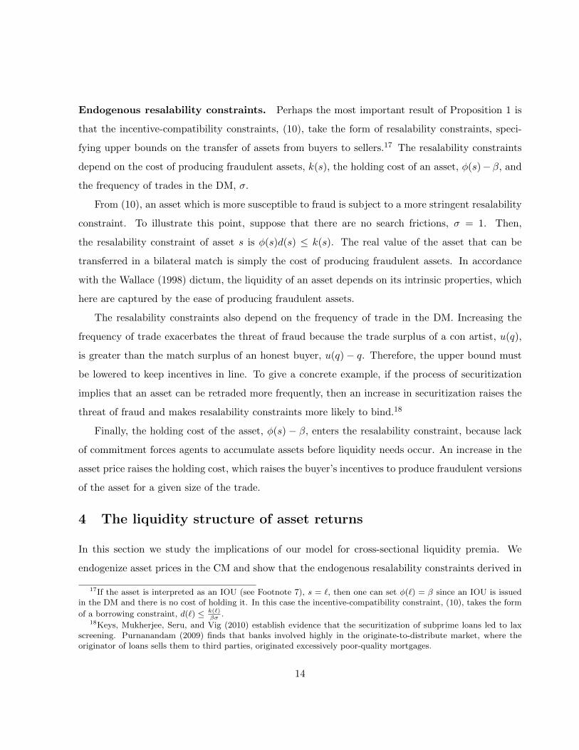
0 κ(s)

asset price

liquidpartially liquidilliquid

κ

β + ξ

β

κ

Figure 2: The liquidity structure of asset returns

The central implication of Proposition 2 is that, whenever there is a liquidity shortage, L < q∗,

assets with identical cash flows can have different prices. See Figure 2 for a graphical representation

of these price differences. This departure from the no-arbitrage principle is another formulation of

the rate-of-return dominance puzzle, according to which monetary assets coexist with other assets

with similar risk characteristics that generate a higher yield. In our model price differentials across

assets are attributed to differences in the cost of fraud. An asset which is more recognizable—

in the sense of not being sensitive to fraudulent activities—as captured by a high cost of fraud,

is used more intensively to finance random spending opportunities. Relative to assets that are

less recognizable, this asset generates some non-pecuniary liquidity services, ν(s) = φ(s) − β, also

referred to as a convenience yield, and is sold at a higher price.22

Krishnamurthy and Vissing-Jorgensen (2010, 2011) document the existence of convenience

yields for Treasury securities and, to a lesser extent, highly-rated bonds. They argue that a safety-

22To see why the price differentials do not represent arbitrage opportunities, relax the short-selling constraint andassume that, in order to sell an asset he does not own, an agent has to borrow it from someone else in exchange for afee, to be determined in equilibrium. The agent who borrows the asset can use it in the DM, but the agent who lendsit cannot. The equilibrium remains unchanged, and the fee clearing the market for borrowing asset s ∈ S is equal toits convenience yield, φ(s)− β. Indeed, an agent who borrows a liquid or partially liquid asset must compensate thelender for his forgone liquidity services in the DM.

18

premium (which they view as distinct from a standard risk premium) is an important component of

asset prices. Through the lens of our model, we can interpret this safety premium as the premium

offered by assets that are highly recognizable and that are less sensitive to informational asym-

metries and moral hazard considerations. Similarly, Vickery and Wright (2010) argue about the

existence of a liquidity premium for agency mortgage-backed securities, which are better protected

against the informational asymmetries that plague the process of securitization.

Proposition 2 also has insights for cross-sectional differences in transaction velocity, a standard

measure of liquidity in monetary economies. In our model, transaction velocity in the DM is

V(s) ≡ σd(s)A(s) = σθ(s). Proposition 2 predicts a positive relationship between the price of an asset

and its velocity. The most liquid assets (i.e., any asset s such that κ(s) ≥ κ) trade at the highest

price, and their velocity is maximum and equal to the frequency of spending opportunities in the

DM, σ. Illiquid assets (i.e., any asset s such that κ(s) <κ), however, have the highest rate of return,

equal to the rate of time preference, and the lowest velocities, less than σ. This result is consistent

with the view that bonds that are used more intensely as collateral in OTC markets tend to have

higher prices (Duffie, 1996).

In reality, a myriad of assets are not used as means of payment or collateral. This observation

is consistent with our results if there is a mass of assets that do not circulate in the DM, θ(s) = 0.

From (21) such assets must be characterized by κ(s) = 0: these are assets for which agents have so

little knowledge about their mere existence or attributes, that even simple, costless frauds can be

deceptive.23

5 Applications and Extensions

In this last section we apply our model of the liquidity structure of asset returns to analyze flight-

to-liquidity phenomena and to assess the effectiveness of aggregate liquidity management policies.

Moreover, we extend the model to an infinite time horizon in order to study time variations in

liquidity premia.

23That assets, or claims on those assets, can be counterfeited at no cost has been the standard explanation inmonetary theory for why capital goods are illiquid, since Freeman (1985), and more recently, Lester, Postlewaite, andWright (2011).

19

5.1 Flights to liquidity

A flight to liquidity occurs when market participants seek to reallocate their portfolios toward

highly liquid assets, which leads to a widening yield spread between liquid and less liquid assets.24

In what follows, we apply our analysis on the liquidity structure of asset returns to identify the

shocks that can generate a simultaneous increase in the prices of the most-liquid assets and a

reduction in the prices of less-liquid ones—a phenomenon resembling a flight to liquidity.

According to our model, a flight to liquidity can be explained by an exogenous reduction in k(s)

for some initially liquid or partially liquid assets that make them become illiquid. For instance,

agents might realize that some assets (e.g., MBS) can be subject to a broader set of fraudulent

practices than previously thought.25 The resalability and velocity of these assets decrease, which

causes aggregate liquidity and output to fall, and the liquidity premium on liquid assets, ξ, to

increase.26 The prices of partially liquid assets do not change, except for the ones that are charac-

terized by a lower cost of fraud. In addition, an increase in the threat of fraud can shrink the set

of liquid assets, while it expands the set of illiquid and partially liquid ones. Indeed, the threshold

κ = βσ + ξ and the interval κ− κ = ξ are increasing functions of the size of the liquidity premium

on liquid assets. Therefore, during a flight to liquidity, market demand for assets is concentrated

on a smaller set of highly recognizable assets.

An alternative explanation for a flight to liquidity is an increase in σ that formalizes an aggregate

liquidity demand shock, e.g., an increase in counterparty risk, leading to an increase in the demand

for collateral for OTC transactions.27 From (16) and (18) when σ increases the prices of liquid

24During the 1998 Russian-default crisis, many investors shifted their funds into the more liquid U.S. Treasurymarket, widening the yield spread between Treasury bonds and less-liquid debt instruments (Longstaff, 2004). Ev-idence also shows that, during the subprime crisis, the flight-to-quality was confined to AAA-rated bonds, and theilliquidity component of the rate of return of bonds with lower grades rose sharply (Longstaff, 2010; Dick-Nielsen,Feldhutter, and Lando, 2010).

25For some prominent economists this type of shock is a central explanation for the financial crisis of 2008. Inan interview to the Wall Street journal (09/24/2011), Robert Lucas argued that ”the shock came because complexmortgage-related securities minted by Wall Street and certified as safe by rating agencies had become part of theeffective liquidity supply of the system. All of a sudden, a whole bunch of this stuff turns out to be crap”.

26Some recent studies (e.g., Ajello, 2010; Shi, 2011) formulate the hypothesis that recessions are driven by liquidityshocks formalized by a reduction in the exogenous resalability of some assets. In contrast to our approach, thesemodels have the counterfactual implication that the prices of the assets that become more difficult to resell increase.

27Suppose, for instance, that a fraction σu of the trades in the DM can be financed with unsecured debt (e.g.,because commitment/enforcement is available in those meetings) while a fraction σs of the trades require collateralto be posted because of counterparty risk (e.g., sellers in those meetings cannot commit or cannot be forced to repay

20

assets rise, whereas the prices of partially liquid assets fall. The increase in the prices of liquid

assets occurs due to two effects going in the same direction. There is a direct effect according

to which liquid assets are used more often as collateral or means of payment, which raises their

liquidity value. The indirect effect is to reduce aggregate liquidity: from (15), an increase in σ

lowers the weights of illiquid assets in L, which reduces the output in bilateral matches and makes

liquid assets even more useful; i.e., the term β [u�(q)− 1] in (12) goes up. For partially liquid assets

the increase in σ has the additional markedly different effect of exacerbating fraud incentives. As

a result, their prices have to fall so that their resalability constraints hold, re-establishing buyers’

incentives to bring genuine assets. As shown in Figure 2, the set of illiquid and partially liquid

assets expands (because κ increases with σ and κ−κ increases with ξ) while the set of liquid assets

shrinks (because κ increases in ξ).

5.2 Liquidity management

In this section we use our model to study the effectiveness of policies aimed at managing the

supply of liquidity in the economy. These policies can take the form of open-market operations by

the central bank, which are intended to substitute liquid assets for less-liquid ones, or regulatory

measures that reduce the threat of frauds and relax resalability constraints for some assets.

Measuring the social value of assets’ liquidity services. Much of the analysis that follows is

based on the following theoretical observation. In competitive models with reduced-form demand

for liquidity (e.g., cash-in-advance or money-in-the-utility function), the convenience yield of an

asset not only measures the marginal private value of its liquidity services, but also its marginal

social value.28 In our model this property holds true for illiquid and liquid assets, but fails to hold

for partially liquid assets.

The marginal social value of the liquidity services provided by a unit of asset s is ∂L∂A(s)ξ,

which is equal to ξ for liquid and partially liquid assets, and 0 for illiquid assets. Therefore, the

convenience yield of partially liquid assets, φ(s) − β < ξ, underestimates the true marginal social

their debt.) An increase in counterparty risk can be formalized as an increase in σs such that σs + σu is unchanged.28This logic is underlying the calculation for the welfare cost of inflation in Lucas (2000), the measure of the

liquidity services provided by Treasuries in Krishnamurthy and Vissing-Jorgensen (2010), and Barnett, Fisher, andSerletis’s (1992) definition of Divisia monetary aggregates.

21

value of their liquidity services. The reason for this discrepancy is that an increase in the price of

an asset reduces its demand in two ways: by raising the holding cost, φ(s)− β, and by tightening

the resalability constraint. The latter effect creates a negative “pecuniary externality,” which can

depress asset prices below the marginal social value of the asset’s liquidity services.29 As we show

below, this observation implies that liquidity management policies targeting partially liquid assets

can be welfare reducing, because they underestimate these assets’ true contribution to aggregate

liquidity. By contrast, when targeting illiquid assets, the same policies are welfare improving.

Open-market purchases. Central banks routinely engage in aggregate liquidity management,

by issuing (or withdrawing) reserves, the most liquid assets, in exchange for Treasuries and, in recent

years, a wider range of less liquid assets, including agency bonds and mortgage-backed securities.

Consider a policy-maker in the CM, who sells a quantity, ∆A(s), of some liquid asset s from his

portfolio, and simultaneously purchases a quantity, ∆A(s�), of some other asset s�. A small open-

market operation has a small effect on prices, so that the budget constraint of the policy-maker is,

to a first-order approximation, φ(s)∆A(s) +φ(s�)∆A(s�) = 0. The welfare effect of such a policy is

∆L× ξ =

�∂L

∂A(s)∆A(s) +

∂L

∂A(s�)∆A(s�)

�ξ =

�1− ∂L

∂A(s�)

φ(s)

φ(s�)

�∆A(s)× ξ.

Suppose first that κ(s�) > κ, so both s and s� are liquid assets. Then, φ(s) = φ(s�), ∂L∂A(s�) = 1,

and ∆L = 0. Such an open-market operation is irrelevant: it does not change aggregate liquidity

and welfare, and hence it has no effect on output and asset prices. So liquidity management has

real effects only if it involves assets with different degrees of liquidity.

Suppose next that κ(s�) <κ, asset s� is illiquid. In this case aggregate liquidity does increase

because the purchase of illiquid assets has no consequence on aggregate liquidity; i.e., ∆L × ξ =

∆A(s)× ξ > 0. Thus, welfare increases, the price of liquid assets decreases, and the price of illiquid

assets is unaffected.

Finally, suppose that κ(s�) ∈ (κ, κ) ; i.e., asset s� is partially liquid. Then, φ(s�) < φ(s) and

∆L × ξ =�1− φ(s)

φ(s�)

�∆A(s) × ξ < 0, implying that such a policy reduces aggregate liquidity and

29By contrast, with the exogenous proportional resalability constraint, there is no such pecuniary externality, andasset convenience yields coincide with the marginal social value of the asset’s liquidity services. See SupplementaryAppendix E.

22

welfare. The intuition is in line with our earlier observation: while partially liquid and liquid assets

have different prices, they contribute equally to aggregate liquidity. At the same time, because it

has a higher price, one share of a liquid asset buys more than one share of a partially liquid one.

Thus a balanced-budget open-market operation ends up syphoning out more liquidity than it is

injecting in; i.e., aggregate liquidity is reduced. The welfare effect of this open-market operation is

of the opposite sign of the yield difference between the asset that is withdrawn and the asset that

is injected, and the prices of both assets s and s� increase.

The results above can help interpret some of the findings in Krishnamurthy and Vissing-

Jorgensen (2011) regarding the effect of quantitative easing. They find that the purchases of

Treasuries, agency bonds, and highly-rated corporate bonds in exchange for reserves led to a drop

in interest rates but it did not affect the yields on relatively illiquid assets (Baa corporate bonds).

This finding is consistent with our results if we interpret Baa corporate bonds as illiquid assets,

Treasuries and highly rated bonds as partially liquid, and reserves as fully liquid. Furthermore,

according to our findings, the drop in interest rates indicates that quantitative easing reduced

liquidity and welfare.

Regulatory measures. Some of the leading regulatory measures of the Dodd-Frank Act aim

to curb fraud incentives in the securitization industry.30 One of these measures is a requirement

for securitizers to retain at least 5 percent of the credit risk they originate. Importantly, some

asset-backed securities, deemed of higher quality, are exempted from this requirement. In this

section, we study the optimality and welfare impact of retention requirements. We show that the

regulator faces a trade-off between the role these requirements play as a discipline mechanism and

the distortion they introduce by increasing the costs of holding assets. We demonstrate that the

first effect dominates for illiquid assets, while the second effect dominates for partially liquid and

liquid assets. Hence, our model suggests that retention requirements should be confined to the least

liquid assets, i.e., the ones more susceptible to fraud.

Under a retention requirement policy, a buyer who wishes to transfer d(s) units of asset s in

the DM must hold 1 + ρ(s) units of the asset; i.e., d(s) ≤ a(s)1+ρ(s) , where ρ(s) is the retention rate

30The Dodd-Frank Act, enacted in July 2010 in response to the 2007-08 financial crisis, institutes a wide array ofnew regulations for the financial services industry.

23

associated with asset s. The policy imposes that the asset kept in retention is the exact same

asset as the one transferred in a match, i.e., if the asset transferred is fraudulent, so is the asset in

retention.31 The cost of producing d(s) units of fraudulent asset is of the form kf (s) + kv(s)d(s),

where the variable cost component, kv(s)d(s), was introduced to provide a channel through which

the regulatory measure can reduce agents’ incentive to commit fraud. We let kf (s) > 0 and take

kv(s) to be small enough so that, as before, equilibrium offers are accepted with probability one

(see Supplementary Appendix B). The resalability constraint of asset s becomes:

kf (s) + kv(s) [1 + ρ(s)] d(s) ≥ [φ(s)− β] [1 + ρ(s)] d(s) + βσd(s). (22)

The left side of (22) is the cost of fraud on d(s) units of asset s. If kv(s) > 0, then policy increases

the cost of fraud and, therefore, reduces fraud incentives. The right side of (22) is the cost of holding

[1 + ρ(s)] d(s) genuine units of asset s. Thus, if the asset is liquid or partially liquid, φ(s)− β > 0,

the retention requirement generates a distortion by increasing the effective holding cost of the asset.

In Supplementary Appendix B, we solve for equilibrium following the same steps as before. We

show that a retention requirement has asymmetric effects on the resalability of an asset, depending

on its liquidity status. For illiquid assets, equilibrium resalability becomes:

θ(s) =kf (s)/A(s)

βσ − kv(s) [1 + ρ(s)]. (23)

It is an increasing function of ρ(s) because when φ(s) = β retention rates raise the cost of com-

mitting fraud but do not affect assets’ effective holding costs. For liquid and partially liquid assets

resalability becomes:

θ(s) =1

1 + ρ(s), (24)

which is a decreasing function of ρ(s). Thus, for liquid or partially liquid assets, the distortionary

effect of retention rates dominates the incentive effect, reducing velocity and welfare. In the case of

liquid assets, this result is straightforward since the threat of fraud is not a binding constraint. In the

case of partially liquid assets, retention requirements have the partial equilibrium effect of relaxing

resalability constraints. But this effect simultaneously increases the demand for partially liquid

31In the context of securitization (see Supplementary Appendix H), a retention requirement means that thesecuritizer (represented in the model by the buyer) needs to retain assets from the same issue of asset-based securitieshe is offering to the general public (represented in the model by the seller).

24

assets. Therefore, for asset markets to clear, the prices of partially liquid assets must increase,

tightening back the resalability constraints and eliminating the positive incentive effect of the

retention policy. Taken together, the above results suggest that retention requirements should target

illiquid assets. Other, more recognizable assets, should be exempted, in line with the prescriptions

of the Dodd Frank Act.

5.3 Dynamics of liquidity premia

This section provides a dynamic extension of our static model. We show that the prices of all

liquid assets covary with a common liquidity premium.32 This common liquidity premium can be

the subject of self-fulfilling fluctuations, creating excess volatility in the price of liquid assets. The

prices of illiquid and partially liquid assets are, however, immune to such fluctuations.

Given agents’ quasilinear preferences, it is straightforward to introduce an infinite time horizon

using the setup of Lagos and Wright (2005). Time is indexed by t ∈ N. Each period is divided into

two subperiods, a DM followed by a CM. Each unit of the asset s pays off a dividend normalized

to one unit of the numeraire at the beginning of each CM. The technology to produce fraudulent

assets in period t− 1 becomes obsolete in period t, and all fraudulent assets produced in period t

are confiscated by the government before agents enter the CM of period t.33

As shown in supplementary Appendix D, these assumptions allow us to apply the analysis of

the static model, where the terminal value of the asset is equal to the cum-dividend value, 1+φt(s),

of reselling the asset in the CM in period t. Focusing on equilibrium with qt < q∗, Proposition 2

generalizes as follows.34 There are three classes of assets, of which the prices solve:

φt−1(s) = [1 + φt(s)]×

β + ξt κt(s) ≥ κtβ + [κt(s)− βσ] if κt(s) ∈ (κ, κt)β κt(s) ≤ κ

, (25)

32References on the empirical literature on the co-movements of liquidity across assets are included in Acharyaand Pedersen (2005) who develop an asset pricing model in which a per-share cost of selling securities can vary overtime.

33This assumption, borrowed from Nosal and Wallace (2007), is made for tractability to prevent fraudulent assetsfrom circulating across periods.

34If aggregate liquidity is abundant, there exists a unique equilibrium in which the resalability constraint andthe feasibility constraint do not bind at any date, qt = q∗, and each asset is priced at its fundamental value; i.e.,φt(s) = 1/r.

25

where κt(s) ≡ k(s)[1+φt(s)]A(s) , κ ≡ βσ, κt ≡ ξt + βσ, and

ξt = βσ�u�(qt)− 1

�(26)

qt = L =�

s∈Sθt(s) [1 + φt(s)]A(s), where θt(s) = min

�1,

κt(s)

βσ

�. (27)

The equilibrium equations are the same as in the static model, but with an endogenous terminal

value of 1 + φt(s). This difference is substantial because expectations of future liquidity premia,

capitalized in φt(s), feed back into the current liquidity premium, φt−1(s)− β [1 + φt(s)].35

We now characterize equilibria in a neighborhood of the unique steady state,�{φ(s)}, q, ξ

�. In

such a neighborhood, the sets of liquid, partially liquid, and illiquid assets do not change. Moreover,

from (25), one can verify that dφt−1(s)dφt(s)

∈ [0, 1) for all κt(s) < κt, so that the prices of illiquid and

partially liquid assets are equal to their steady-state values in any dynamic equilibrium. This need

not be the case for liquid assets. To see this point, let us linearize the equilibrium equations near

the steady state. We obtain, from (25), that the price of liquid assets solves:

φt−1(s) =�β + ξ

�φt(s) +

�φ(s) + 1

�ξt, (28)

where φt(s) ≡ φt(s)− φ(s) and ξt ≡ ξt− ξ. The first term on the right side of (28) is the discounted

value of the future price of the asset, with the discount rate augmented by a liquidity premium;

the second term captures the change in the liquidity premium. Linearizing (26) and (27) in the

neighborhood of the steady state:

ξt = βσu��(q)qt where qt =�

s:κ(s)≥κ

φt(s)A(s), (29)

and qt ≡ qt − q. From (29), the size of the liquidity premium, relative to its steady-state value,

depends negatively on changes in the market capitalization of liquid assets.

Multiplying both sides of (28) by A(s) and taking the sum over all liquid assets, we obtain

ξt−1 = γξt, where γ = β + ξ + βσu��(q)�

s:κ(s)≥κ

�φ(s) + 1

�A(s). (30)

35This effect, as is well known, can lead to an equilibrium in which an asset has positive value even if it pays nodividend; i.e., a positive liquidity premium can be a self-fulfilling phenomenon. In Supplementary Appendix D weconsider such an economy with fiat money.

26

The nature of the dynamics depends on γ. If γ > −1, then ξt = ξ for all t, and the liquidity

premium is constant over time. If γ < −1, in contrast, there exists a continuum of equilibria

indexed by the initial value of ξ in the neighborhood of zero that converges to the steady state.

Along these equilibria, ξt alternates between positive and negative values. The price of liquid assets

covaries and exhibits excessive volatility relative to fundamentals, whereas the prices of partially

liquid assets and illiquid ones remain constant. As can be seen from (29), the fluctuating liquidity

premium is a self-fulfilling phenomenon. If agents anticipate that the liquidity premium will be

high in the future so that φt > 0, then aggregate liquidity and output are high, qt > 0. But, at

the margin, agents do not value much the asset’s liquidity services, and so the current liquidity

premium is low, ξt < 0. If the constant multiplying ξt in (28) is large enough, then φt−1 < 0. The

same reasoning implies that the liquidity premium one period before will be high, ξt−1 > 0, and

the fluctuations will continue.

6 Conclusion

In this paper we have proposed a theory of the cross-sectional distribution and time-variation of

liquidity premia by taking seriously the possibility of asset fraud in an economy with limited com-

mitment and enforcement. We have shown the emergence of asset-specific resalability constraints

that take the form of upper bounds on the transfer of assets in OTC market trades. These bounds

are not invariant to policy shifts (e.g., the composition of asset supplies and regulation on assets’

retention requirements), and they depend on some characteristics of the assets such as their vulner-

ability to fraud, as well as the frequency of trading opportunities. Our model generates a liquidity

structure of asset returns based on a three-tier classification of assets. This classification is rele-

vant for the comparative statics of asset prices, the dynamics of liquidity premia, explanations of

flight-to-liquidity phenomena, and the analysis of open-market operations and regulations of the

OTC market.

27

References

[1] Ajello, Andrea (2010). “Financial Intermediation, Investment Dynamics and Business Cycle,”

manuscript.

[2] Acharya, Viral V. and Lasse Heje Pedersen (2005). “Asset Pricing with Liquidity Risk,” Journal

of Financial Economics, Elsevier 77, 375-410.

[3] Amihud, Yakov and Haim Mendelson (1986). “Asset Pricing and the Bid Ask Spread,” Journal

of Financial Economics 17, 223-249.

[4] Barnett, William A., Douglas Fisher, and Apostolos Serletis (1992). “Consumer Theory and

the Demand for Money,” Journal of Economic Literature 30, 2086-2119.

[5] Chordia, Tarun, Huh Sahn-Wook and Avanidhar Subrahmanyam (2009). “Theory-Based Illiq-

uidity and Asset Pricing,” Review of Financial Studies 22, 3629-3668.

[6] Dick-Nielsen, Jens, Peter Feldhutter, and David Lando (2010). “Corporate Bond Liquidity

Before and After the Onset of the Subprime Crisis,” manuscript.

[7] Duffie, Darell (1996). “Special Repo Rates” Journal of Finance 51, 493-526.

[8] Duffie, Darrell, Nicolae Garleanu and Lasse Heje Pedersen (2005). “Over-the-counter Markets,”

Econometrica 73, 1815-1847.

[9] Freeman, Scott (1985). “Transactions Costs and the Optimal Quantity of Money,” Journal of

Political Economy 93, 146-157.

[10] Green, Edward and Warren Weber (1996). “Will the New $100 Bill Decrease Counterfeiting?”

Federal Reserve Bank of Minnepolis Quarterly Review 20, 3-10.

[11] Guerrieri, Veronica and Robert Shimer (2011). “Dynamic Adverse Selection: A Theory of

Illiquidity, Fire Sales, and Flight to Quality,” mimeo.

[12] Guerrieri, Veronica, Robert Shimer, and Randall Wright (2010). “Adverse Selection in Com-

petitive Search Equilibrium,” Econometrica 78 , 1823-1862.

28

[13] Holmstrom, Bengt and Jean Tirole (2011). Inside and Outside Liquidity, Princeton, Princeton

University Press.

[14] Hopenhayn, Hugo A. and Ingrid M. Werner (1996). “Information, Liquidity, and Asset Trading

in a Random Matching Game,” Journal of Economic Theory 68, 349-379.

[15] In, Younghwan and Julian Wright (2011). “Signaling Private Choices,” manuscript.

[16] Keys, Benjamin J., Tanmoy K. Mukherjee, Amit Seru, and Vikrant Vig (2010). “Did secu-

ritization lead to lax screening? Evidence from subprime loans,” The Quarterly Journal of

Economics 125, 307-62.

[17] Kiyotaki, Nobuhiro and John Moore (2001). “Liquidity, Business Cycles and Monetary Policy,”

manuscript.

[18] Kiyotaki, Nobuhiro and John Moore (2005). “Liquidity and asset prices,” International Eco-

nomic Review 46, 317-349.

[19] Kohlberg, Elon and Jean-Francois Mertens (1986). “On the strategic stability of equilibria,”

Econometrica 54, 1003-1037.

[20] Krishnamurthy, Arvind and Annette Vissing-Jorgensen (2010). “The aggregate demand for

Treasury debt,” manuscript.

[21] Krishnamurthy, Arvind and Annette Vissing-Jorgensen (2011). “The Effects of Quantitative

Easing on Interest Rates,” manuscript.

[22] Lagos, Ricardo (2010). “Asset prices and liquidity in an exchange economy,” Journal of Mon-

etary Economics 57, 913-930.

[23] Lagos, Ricardo and Randall Wright (2005). “A unified framework for monetary theory and

policy analysis,” Journal of Political Economy 113, 463–484.

[24] Lester, Benjamin, Andrew Postlewaite and Randall Wright (2011). “Information, Liquidity,

Asset Prices, and Monetary Policy,” Review of Economic Studies, forthcoming.

29

[25] Longstaff, Francis A. (2004). “The Flight-to-Liquidity Premium in U.S. Treasury Bond Prices,”

Journal of Business 77, 511-526.

[26] Longstaff, Francis A. (2010). “The subprime credit crisis and contagion in financial markets,”

Journal of Financial Economics 97, 436-450.

[27] Lucas, Robert E. (2000). “Inflation and Welfare,” Econometrica 68, 247-274.

[28] Friedman, Milton and Anna J. Schwartz (1970). Monetary statistics of the United States:

estimates, sources, methods, NBER Studies in business cycles, no. 20, New York: National

Bureau of Economic Research.

[29] Mihm, Stephen (2007). A nation of counterfeiters: Capitalists, con men, and the making of

the United States, Cambridge, Harvard University Press.

[30] Nosal, Ed and Neil Wallace (2007). “A model of (the threat of) counterfeiting,” Journal of

Monetary Economics 54, 229-246.

[31] Purnanandam, Amiyatosh K. (2009). “Originate-to-Distribute Model and the Subprime Mort-

gage Crisis,” manuscript.

[32] Rocheteau, Guillaume (2009). “A Monetary Approach to Asset Liquidity,” Working Papers

09-01, Federal Reserve Bank of Cleveland.

[33] Sargent, Thomas J. and Francois R. Velde (2002). The Big Problem of Small Change, Prince-

ton: Princeton University Press.

[34] Schreft, Stacey L. (2007). “Risks of identity theft: Can the market protect the payment sys-

tem?” Federal Reserve Bank of Richmond, Economic Review, Fourth Quarter, 5-40.

[35] Shi, Shouyong (2008). “Efficiency improvement from restricting the liquidity of nominal

bonds,” Journal of Monetary Economics 55, 1025– 1037.

[36] Shi, Shouyong (2011). “Liquidity, Assets and Business Cycles,” manuscript.

30

[37] Snowden, Kenneth A. (2010) “Covered Farm Mortgage Bonds in the Late Nineteenth Century

U.S,” NBER Working Papers 16242

[38] Vickery, James and Joshua Wright (2010). “TBA Trading and Liquidity in the Agency MBS

Market,” manuscript.

[39] Wallace, Neil (1998). “A dictum for monetary theory,” FRB Minneapolis Quarterly Review

22: 20-26.

[40] Wallace, Neil (2000). “A model of the liquidity structure based on asset indivisibility,” Journal

of Monetary Economics 45, 55-68.

[41] Weill, Pierre-Olivier (2008). “Liquidity premia in dynamic bargaining markets,” Journal of

Economic Theory 140, 66-96.

[42] Williamson, Stephen and Randall Wright (1994). “Barter and Monetary Exchange under Pri-

vate Information,” American Economic Review 84, 104-123.

31

A Proof of Proposition 1

We define an outcome of the game as an offer (q, {d(s)}) made by the buyer, probabilities {η(s)} of

bringing genuine assets, and a probability π ∈ [0, 1] that the seller accepts the offer. Let us consider

the auxiliary problem of choosing an outcome in order to maximize the expected utility of a buyer,

−�

s∈S

�k(s) [1− η(s)] + [φ(s)− β] η(s)d(s)

�+ σβπ

�u(q)−

�

s∈Sη(s)d(s)

�, (31)

subject to the constraint that the probabilities π and {η(s)} are the basis of an equilibrium in the

sub-game following offer (q, {d(s)}); that is:

π ∈ arg maxπ∈[0,1]

π

�− q +

�

s∈Sη(s)d(s)

�(32)

η(s) ∈ arg maxη∈[0,1]

η

�k(s)− [φ(s)− β + βσπ] d(s)

�, for all s ∈ S. (33)

We start by showing that:

Claim 1 Any solution of the auxiliary problem has the property that η(s) = 1 and q =�

s∈S d(s).

Proof. Consider first any feasible outcome �q, d, η,π� such that η(s0) < 1 for some s0. If

η(s0) = 0, then consider the alternative outcome, �q�, d�, η�,π��, such that: (i) q� = q, d�(s) = d(s)

for all s �= s0, d�(s0) = 0; (ii) η�(s) = η(s) for all s �= s0 and η�(s0) = 1; (iii) π� = π. The

incentive constraint of the seller, (32), is satisfied since it only depends on the product η(s)d(s).

The incentive constraint of the buyer, (33), is obviously satisfied for s �= s0. For s = s0 we have

k(s0) > [φ(s)− β + βσ] d�(s0) = 0 and so η�(s0) = 1 is optimal for the buyer. One can then verify

that, with this alternative outcome, the expected utility of the buyer increases by k(s0) > 0.

Next, consider any feasible outcome such that η(s0) ∈ (0, 1): the buyer is indifferent between

counterfeiting asset s0 or not. We then increase η(s0) by ε ∈ (0, 1] and q by εd(s0), which is positive

since the incentive constraint of the buyer, (33), binds. The incentive constraint of the seller, (32)

is satisfied because his payoff conditional on accepting the offer does not change. Because the buyer

is indifferent between counterfeiting asset s0 or not, an increase in η(s0) affects neither his payoff,

(31), nor his incentive constraint, (33). The corresponding increase in q, however, increases his

payoff strictly.

32

Next, consider any feasible outcome �q, d, η,π� such that η(s) = 1 for all s, but q <�

s∈S d(s).

Then the alternative outcome with q� =�

s∈S > q, η�(s) = 1, and π� = π, increases the expected

payoff to the buyer by σβπ [u(q�)− u(q)] > 0 and satisfies all the constraints.

This claim implies that we can rewrite the auxiliary problem as

maxq,d,π

−�

s∈S[φ(s)− β] d(s) + σβπ [u(q)− q] (34)

s.t.�

s∈Sd(s)− q = 0 (35)

k(s) ≥ [φ(s)− β + βσπ)] d(s), for all s ∈ S. (36)

The second condition is the first-order necessary and sufficient condition for (33) evaluated at

η(s) = 1. Next, we show:

Claim 2 Any solution of the auxiliary problem, (31)-(33), has the property that u�(q) ≥ 1 and

π = 1.

Proof. The first claim holds because otherwise one could reduce the quantity produced, increase

the expected utility of the buyer, and satisfy all the constraints. To prove the second claim suppose,

towards a contradiction, that π < 1. Note first that the value of the auxiliary problem must be

positive: a small offer q� = d�(s0) > 0, d�(s) = 0 for s �= s0, and π� = 1 yields a positive payoff.

This implies that both q > 0 and π > 0. Moreover, at least one of the incentive constraints,

(36), must be binding since otherwise one could increase π without violating any of the incentive

constraints, and improve the objective. Let SB ⊆ S be the set of binding IC constraints. Since

[φ(s)− β + βσπ] d(s) = k(s) for all s ∈ SB, it follows that d(s) > 0. Now consider the following

variational experiment: increase π by some small ε and decrease the payments d(s), for all s ∈ SB,

so that all the incentive constraints continue to bind. Up to second-order terms, the decrease in

d(s) is equal to m(s)ε, where

m(s) ≡ βσd(s)

φ(s)− β + βσπ,

is the marginal rate of substitution between π and d(s) in the IC constraint for asset s ∈ SB.

Lastly, to satisfy the participation constraint, the decrease in q must be, up to second order terms,

33

�s∈SB

m(s)ε. The change in the buyer’s expected utility is, up to second-order terms, equal to

∆U × ε, where

∆U =�

s∈SB

[φ(s)− β]m(s)− βσπ�u�(q)− 1

� �

s∈SB

m(s) + βσ [u(q)− q]

>�

s∈SB

[φ(s)− β]m(s) + βσ�u�(q)− 1

�

q − π�

s∈SB

m(s)

≥�

s∈SB

[φ(s)− β]m(s) + βσ�u�(q)− 1

� �

s∈SB

[d(s)− πm(s)] =�

s∈SB

[φ(s)− β]m(s)u�(q) ≥ 0,

where we move from the first line to the second line using u(q)− q > q [u�(q)− 1] ≥ 0 (the equality

is strict because of two facts: first, u(q) is strictly concave and second, q > 0, since the value of

the auxiliary problem is positive); from the second line to the third line using q ≥�

s∈SBd(s); and

from the third to the fourth line by noting that d(s)− πm(s) = [φ(s)− β]m(s)/(βσ).

From Claims 1-2 and the result according to which a(s) ≥ χ(s)d(s) if φ(s) = β, and a(s) =

χ(s)d(s) if φ(s) > β, it follows that the auxiliary problem, (31)-(33), reduces to the maximization

problem of Proposition 1, (8)-(11). Now we note that the solution to the auxiliary problem is an

upper bound on the value of the buyer in any equilibrium of the game. Let (q, {d(s)}) be one

solution of the auxiliary problem. Because, as argued above, the value of the auxiliary problem

is positive, it must satisfy q > 0 and d(s) > 0 for some s ∈ S. Consider, for any ε > 0 small

enough, the offer dε(s) = max{d(s)− ε, 0} and qε = q− (S+1)ε. By construction, this offer is such

that [φ(s)− β + βσ] dε(s) < k(s), and qε <�

s∈S dε(s). Thus, π = 1 and η(s) = 1 is the unique

equilibrium in the subgame following (qε, {dε(s)}). By letting ε go to zero and making the above

offer, the buyer can achieve a value arbitrarily close to that of the auxiliary problem. Therefore, in

any equilibrium, the buyer’s value must be equal to that of the auxiliary problem. Moreover, any

equilibrium outcome satisfies (32) and (33). Therefore, any equilibrium outcome must solve the

auxiliary problem.

34