i

National Institute for Higher Education,Dublin School of Electronic Engineering

Thesis Submitted for Degree of Master of Engineering

Low Bit Rate Speech Transmission Classified Vector Excitation Coding

By

Brian F Buggy B E (Hons)

I declare that the research herein was completed by the undersigned

Submitted to

Dr Sean Marlow B Sc PhD

August 1987

Signed Date

TABLE OF CONTENTS

Abstract 1

Acknowledgments 2

1 Introduction 3

2 Predictive Coding of speech 72 1 Introduction 72 2 A Predictive Coding Scheme for Speech, 9 2 3 Prediction Based on Short Time

Spectral Envelope, 102 4 Prediction Based on Spectral Fine

Structure, 13

3 Methods for Determining Linear PredictiveParameters 173 1 Introduction 173 2 Formulation and So lut ion of Linear

Predictor Parameters, 17 3 3 The Autocorrelation Method, 18 3 4 Solution of the Autocorrelation Method 19 3 5 The Formulation and Solution of the

Lattice Method, 22

\

i

3 6 Formulation and Solution of the PitchPredictor Parameters, 25

Implementation and Evaluation of LPC Analysis4 1 Introduction, 314 2 Specification of the LPC Analysis

Parameters, 31 4 3 Comparison of Autocorrelation and Burg

Methods, 33 4 3 1 Stability, 334 3 2 Finite Word Length Effects, 34 4 3 3 Tapered Time Windows, 35 4 3 4 Computational Complexity and

Storage Requirements, 35 4 3 5 Subjective Comparisons, 37 4 3 6 Discussion, 38

4 4 Implementation of the Autocorrelation Method of LPC Analysis, 39

4 5 Analysis of the LPC Analysis and Synthesis Implementation, 45

4 6 Improved Excitation of the LPC Synthesiser, 56

Vector Quantisation 5 1 Introduction, 60 5 2 Preliminaries, 605 3 Formulation of the Codebook Design

Problem, 61 5 4 Motivation for Using Vector

Quantisation, 61 5 5 Algorithms for Codebook Design, 645 6 Vector Quantisation of the LPC

Parameters, 66

Algorithms for Waveform Vector Quantisation6 1 Introduction, 696 2 Waveform Vector Quantisation, 69 6 3 Analysis of a Waveform VQ System using

the LBG Algorithm, 73 6 4 Pairwise Nearest Neighbour Clustering

Algorithm, 776 5 Analysis of the PNN Algorithm 79

Classification of the LPC Residual7 1 Introduction, 827 2 Choice of Classification Parameters, 83 7 3 Classification of Codebook Excited LPC

(CCELP) System, 86

7 4 Simple Classified Residual Vector Excitation (CVXC), 89

7 5 Evaluation of the CVXC System, 93

Improvements and Future Developments 8 1 Introduction, 97 8 2 Improving the Codebook, 97 8 3 Perceptual Noise Weighting, 98 8 4 Incorporation of Multi-Pulse

Codebook Design, 101 8 5 Alternative Search Procedure, 102 8 6 Real Time Implementation, 103

Conelusions

Bibllography

into

Appendix I

Abstract

Vector excitation coding (VXC) is a speech digitisation technique growing in popularity Problems associated with VXC systems are high computational complexity and poor reconstruction of plosives

The Pairwise Nearest Neighbour (PNN) clustering algorithm is proposed as an efficient method of codebook design It is demonstrated to preserve plosives better than the Linde-Buzo-Gary (LBG) algorithm [34] and maintain similar quality to LBG for other speech Classification of the residual is then studied This reduces codebook search complexity and enables a shortcut in computation of the PNN algorithm to be exploited

1

Acknowledgment

I am indebted to Dr S Marlow who kindled my interest in speech processing and enabled me to undertake this research I wish to thank Dr C McCorkell for his encouragement during the last two years and Mr N Murphy for his help in resolving many technical and mathematical problems I would also like to thank Miss M Broderick for her assistance in preparing this thesis

2

The proliferation of wide bandwidth communication systems such as microwave, satellite and optical links has not sated man's appetite for communication Efforts at reducing the bandwidth required for voice transmission, known as speech coding, are now more m demand than ever Speech coding strives to reduce the bandwidth required, through the application of signal processing techniques

The first voice coder or vocoder was invented in the late 1930s However, it was the wide availability of fast computers and the advent of digital signal processing which caused a revolution in speech coding m the 1960s One of the most powerful speech processing techniques called Linear Predictive coding (LPC) was developed independently by Atal and Schroeder [1] and Itakura and Saito [2] at this time It is a source coder i e it attempts to track the underlying process producing the speech wave The algorithm produces a digital filter which approximates the spectra 1 shape of the speech and a residual which is "relatively white"

In an LPC speech coding system, the spectral filter is transmitted along with some information concerning the excitation to be used to re-synthesise the speech The simplest excitation model is to assume only two forms of

1 Introduction

3

speech exist voiced and unvoiced This oversimplification gives synthetic quality results with the most critical element being the choice of voiced/unvoiced threshold The bit rate is low being only about 2400 bit/s

Waveform coding has been applied to the residual to improve quality Scalar quantisation has been used to achieve communication quality with very good results However, the bit rate for good quality transmission is greater than 24,000 bits/s and the complexity is greatly increased

In recent years, efforts have concentrated at producing good quality speech below 9,600 bits/s The motivation for such low bit rates is to reduce the cost of future all-digital telephone equipment as transmission below 9,600 bits/s is feasible on most telephone systems Other applications of growing importance are the incorporation of voice mail within computer systems, the demand for sophisticated encryption of the speech signal and more efficient use of radio frequency bandwidth for cellular telephone systems

One method of achieving good quality around 8k bit/s is to use multi-pulse excitation [3] The complexity of this is very high but the speech generated is highly intelligible Unfortunately, below 8k bits/s, the quality

4

of this system degrades rapidlyMost recently research has concentrated on a form of

coding known as Vector Quantisation (VQ) Using this method code books are generated which attempt to find the best fit for all possible LPC residuals This method has the possibility of transmission at bit rates as low as 4,800 bits/c Code Excited Linear Prediction (CELP) was demonstrated by Atal and Schroeder to give results [4] using Gaussian codebooks but computational costs were prohibitive and reproduction of plosives was very poor

In this thesis, an investigation of Vector Excitation Coding VXC is carried out It starts with a detailed investigation LPC to determine a suitable algorithm to use which will be both robust and give an accurate representation of the speech spectra Two formulations are examined and the autocorrelation method is chosen over the Burg method because it is less computationally intensive and gives comparable results Thecharacteristics of various residuals are examined to demonstrate various critical wave shapes that have to be preserved to achieve good quality coding A majorobjective and a shortcoming of previous algorithms, is the preservation of plosive shape

An investigation of Vector Quantisation and the most popular coding algorithm (K-means) is then undertaken A

5

variation on this algorithm is described for Vector Excitation Coding The limitations of this algorithm, especially in preserving "edges" in the speech is documented An alternative algorithm, known as thePairwise Nearest Neighbours (PNN) clustering algorithm is scrutinised It was previously used in video coding [5] and is reported to preserve "edges" better than the K- means algorithm

Experiments are then performed to find ways of partitioning the codebook so that searching complexity can be reduced This also leads to shortcuts in the codebook design for the PNN algorithm The results of this experimentation are reported for short pieces of test data A system which combines a classified codebook with LPC is proposed (called CVXC) The results obtained are compared with a classified CELP system [6]

Finally, possible alterations and additions are proposed which if carried out should determine the usefulness of the system

6

2 Predictive Coding of Speech

2 1 IntroductionA predictive coder is a system for efficiently

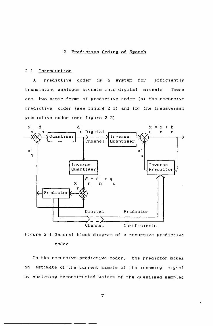
translating analogue signals into digital signals There are two basic forms of predictive coder (a) the recursive predictive coder (see figure 2 1) and (b) the transversal predictive coder (see figure 2 2) x d d ’ Sc = x + b

Figure 2 1 General block diagram of a recursive predictive coder

In the recursive predictive coder, the predictor makes an estimate of the current sample of the incoming signa1 by analysing reconstructed values of the quantised samples

7/

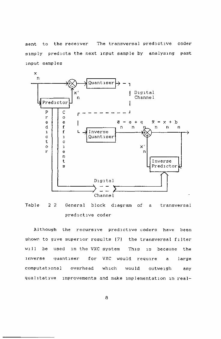
sent to the receiver The transversal predictive coder simply predicts the next input sample by analysing past input samples

x

Table 2 2 General block diagram of a transversal predictive coder

Although the recursive predictive coders have been shown to give superior results [7] the transversal filter will be used in the VXC system This is because the inverse quantiser for VXC would require a large computational overhead which would outweigh any qualitative improvements and make implementation m real­

8

time impracticalTo efficiently apply predictive coding to speech, it is

necessary to take into account the characteristics of this type of signal Speech varies from one sound to anothere g from the unvoiced or noise like /s/ as in "see" tothe voiced and quasi periodic /ee/ Therefore thepredictor must be able to adapt to the change in the input signal This chapter will deal with an examination of predictive systems that exploit certain speech characteristics

2 2 A Predictive Coding Scheme for SpeechPredictive coding schemes for speech have been

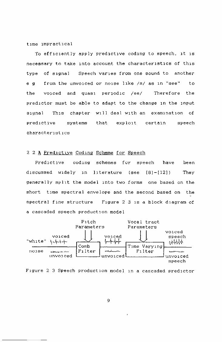
discussed widely in literature (see [8]-[12]) They generally split the model into two forms one based on the short time spectral envelope and the second based on the spectral fine structure Figure 2 3 is a block diagram of a cascaded speech production model

PitchParameters

voiced"white"noise —̂

unvoiced

Xz_Comb Fi Iter

voic e d

unvoiced

Vocal tract Parameters

Time Varying Filter

voicedspeech

unvoicedspeech

Figure 2 3 Speech production model in a cascaded predictor

9

i

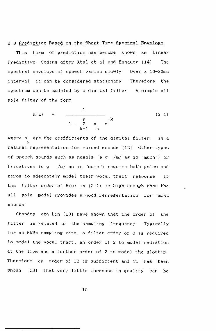
This form of prediction has become known as Linear Predictive Coding after Atal et al and Hanauer [14] The spectral envelope of speech varies slowly Over a 10-20ms interval it can be considered stationary Therefore the spectrum can be modeled by a digital filter A simple all pole filter of the form

1H(z) = (2 1)

P -k1 - 2 a z

k=l kwhere a are the coefficients of the digital filter, is a

knatural representation for voiced sounds [12] Other types of speech sounds such as nasals (e g /m/ as in ‘’much") or fricatives (e g /s/ as in ’’some") require both poles and zeros to adequately model their vocal tract response If the filter order of H(z) in (2 1) is high enough then the all pole model provides a good representation for most sounds

Chandra and Lin [13] have shown that the order of the filter is related to the sampling frequency Typically for an 8kHz sampling rate, a filter order of 8 is required to model the vocal tract, an order of 2 to model radiation at the lips and a further order of 2 to model the glottis Therefore an order of 12 is sufficient and it has been shown [13] that very little increase in quality can be

2 3 Prediction Based on the Short Time Spectral Envelope

10

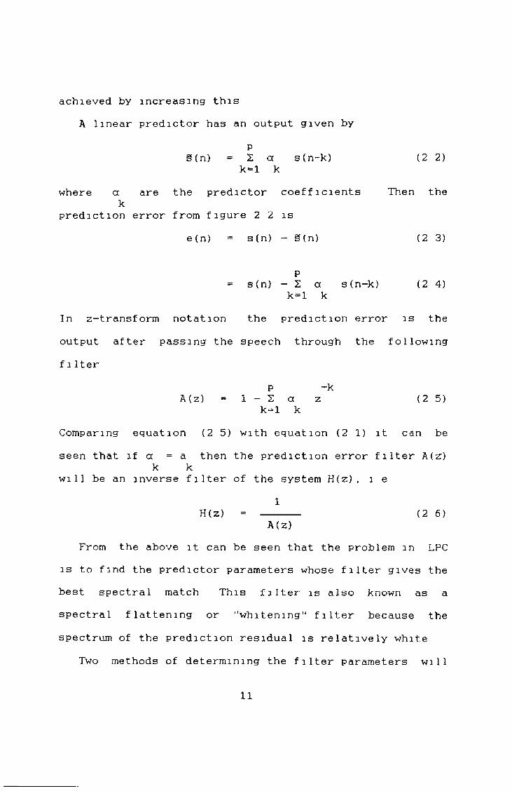
achieved by increasing thisA linear predictor has an output given by

Pg(n) 2 a s(n-k) (2 2)

k*l kwhere a are the predictor coefficients Then the

kprediction error from figure 2 2 is

e (n) s (n) - § (n) (2 3)

P- s(n) - 2 a s(n-k) (2 4)

k=l kIn z-transform notation the prediction error is the output after passing the speech through the following f i Iter

P -kA (z) = 1 - 2 a z (2 5)

k-1 kComparing equation (2 5) with equation (2 1) it can beseen that if a = a then the prediction error filter A(zO

k kwill be an inverse filter of the system H(z), i e

1H(z) = ------- (2 6)

A(z)From the above it can be seen that the problem in LPC

is to find the predictor parameters whose fi 1ter gives the best spectral match This filter is also known as aspectral flattening or "whitening“ filter because the spectrum of the prediction residual is relatively white

Two methods of determining the fi Iter parameters wi11

11

be discussed in sections (3 3) and (3 5)

-1 0 0 0

- i s o o 1- - - - - - - - - 1- - - - - - - - - 1- - - - - - - - -0 0 OS 0 1 0 I1! 0 u 0 time (s)

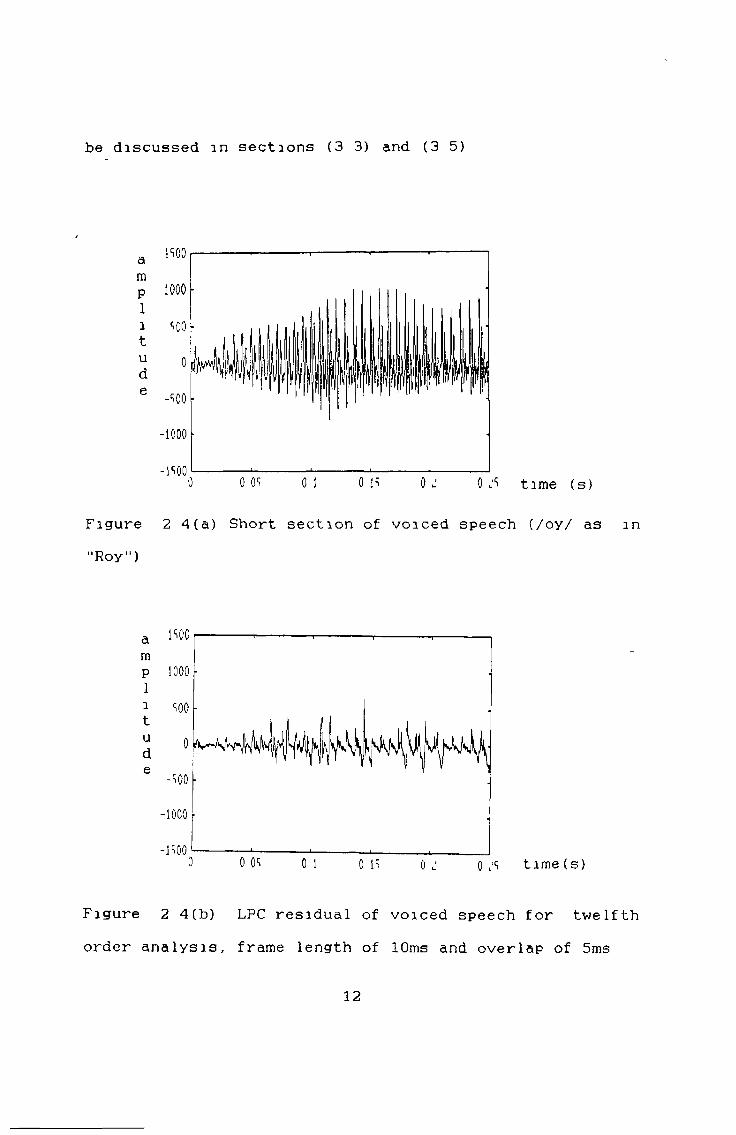
Figure 2 4(a) Short section of voiced speech (/oy/ as "Roy")

amP 1000 ■

1

1 S00 -

-1000 •

-1*500 L .------ ,______o 0 OS 0 1 o IS ft ¿ 0 time (s)

in

Figure 2 4(b) LPC residual of voiced speech for twelfth order analysis, frame length of 10ms and overlap of Sms

12

This is also known as long term prediction or pitch prediction Figure 2 4(a) shows a typical segment of voiced speech The signal is relatively periodic yet after LPC the residual still shows up periodic spikes (figure 2 4(b)) This happens because the LPC only predicts short time spectral shape To remove pitch periodicity, furtherprediction is necessary, but the analysis interval has tobe increased This needs to be done because the lowestpitch frequency found in human speech is approximately 50Hz Therefore a 30ms analysis interval should contain at least one pitch pulse

A simple pitch predictor can be- represented in z- transform notation by

-MP (z) = 3 zd

The delay M of the predictor is the period of theexcitation signal It can be shown (Atal et al [1]) that

< s s > n n-M av

3 = ------- (2 7)<s2 >

n-M avth

where s is the n sample of the excitation signal and n

2 4 Prediction Based on Spectral Fine Structure

1<s s > Z s s (2 8)

n n-M av N n n n-M

13

Figure 2 4(c) Residual of voiced speech (/oy/ as in “Roy") after first order pitch prediction

a 1-00mP 10001

1 SQO

e-*¡00

-1 0 0 0

-I'M0 0 OS 0 1 0 IS 0 J 0 JS time (s)

Figure 2 4(d) Residual of voiced speech (/oy/ as in “Roy“) after third order pitch prediction

14

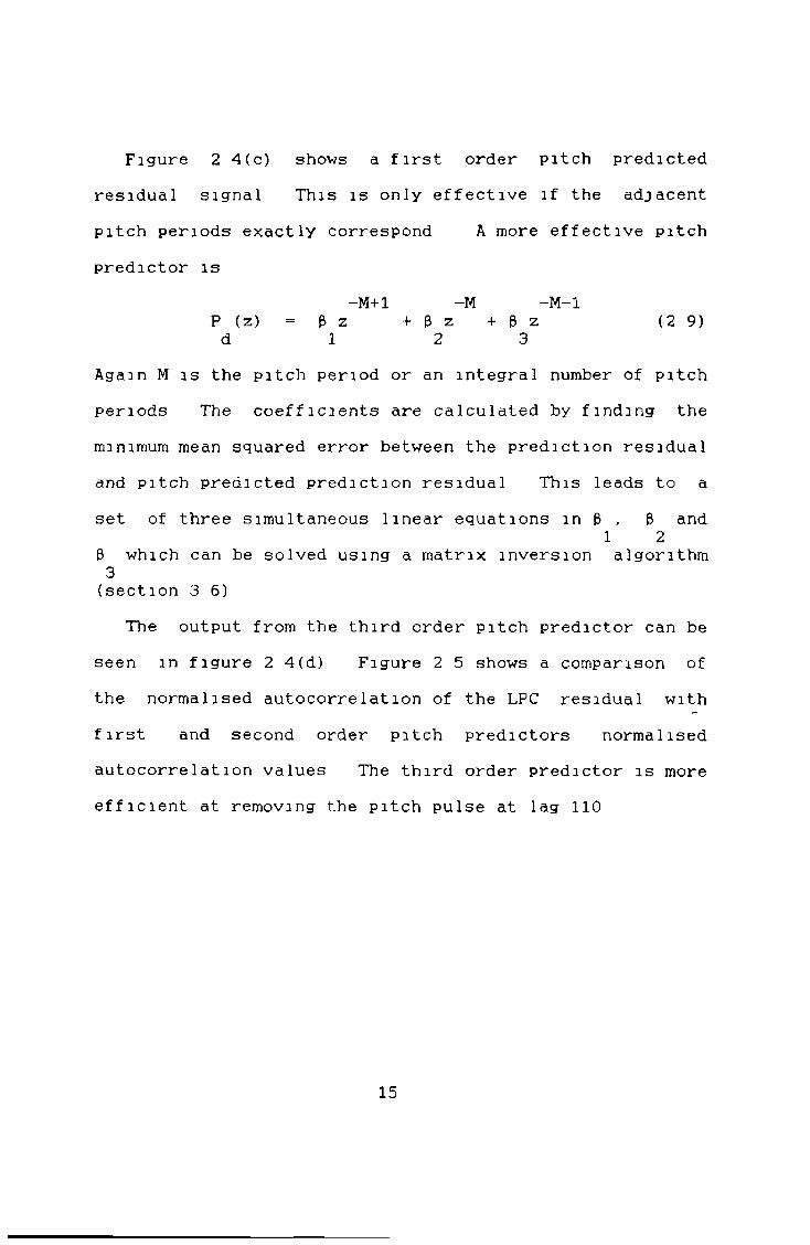
Figure 2 4(c) shows a first order pitch predicted residual signal This is only effective if the adjacent Pitch periods exactly correspond A more effective pitch predictor is

-M+l -M -M -lP (z) = & z + 3 z + 3 z (2 9)d 1 2 3

Again M is the pitch period or an integral number of pitchperiods The coefficients are calculated by finding theminimum mean squared error between the prediction residualand pitch predicted prediction residual This leads to aset of three simultaneous linear equations in 3 , 3 and

1 23 which can be solved using a matrix inversion algorithm 3(section 3 6)

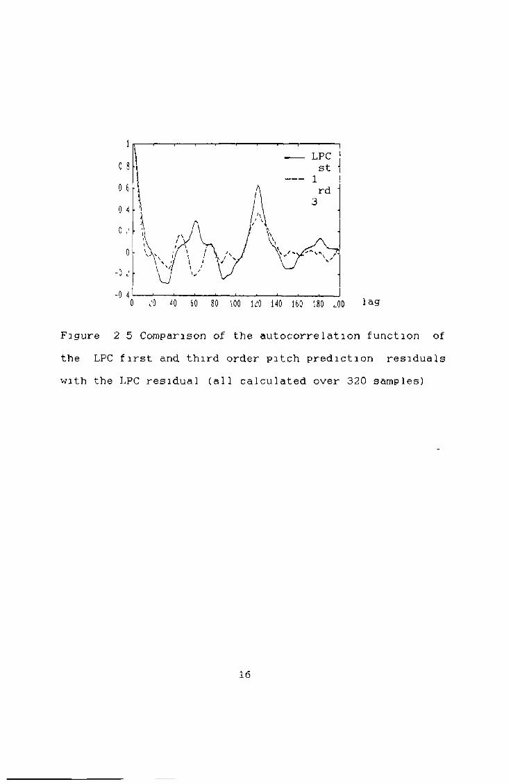
The output from the third order pitch predictor can be seen in figure 2 4(d) Figure 2 5 shows a comparison of the normalised autocorrelation of the LPC residual with first and second order pitch predictors normalised autocorrelation values The third order predictor is more efficient at removing the pitch pulse at lag 110

15

0 8

0 6

0 4 0

0-0 o'

-0 40 t'O 40 60 SO 100 U'O 140 160 180 .0 0

Figure 2 5 Comparison of the autocorrelation function of the LPC first and third order pitch prediction residuals with the LPC residual (all calculated over 320 samples)

1

16

3 Methods for Determining Linear Predictive Parameters

3 1 IntroductionAn overview of Linear Prediction was given in the

previous chapter Here, two formulations will be described, the autocorrelation method and the maximum entropy or Burg method In particular, one algorithm for each formulation wi11 be examined m detai1 These two methods are not the only two available, but they are among the most popular and well understood It is intended that an improved excitation source of a well Known predictive coder will be developed Therefore only well behaved methods will be considered

Finally a long term predictor will be examined and a solution of its parameters will be described

3 2 Formulation and Solution of Linear Predictor Parameters

There are many different formulations of LPC parameters, some of which are listed below

(a) covariance method [14](b) the autocorrelation method [9,15](c) the lattice method [1 0 ](d) the maximum likelihood formulation [15](e) Prony’s method [15]

The first three are the most widely used, but only (b) and

17

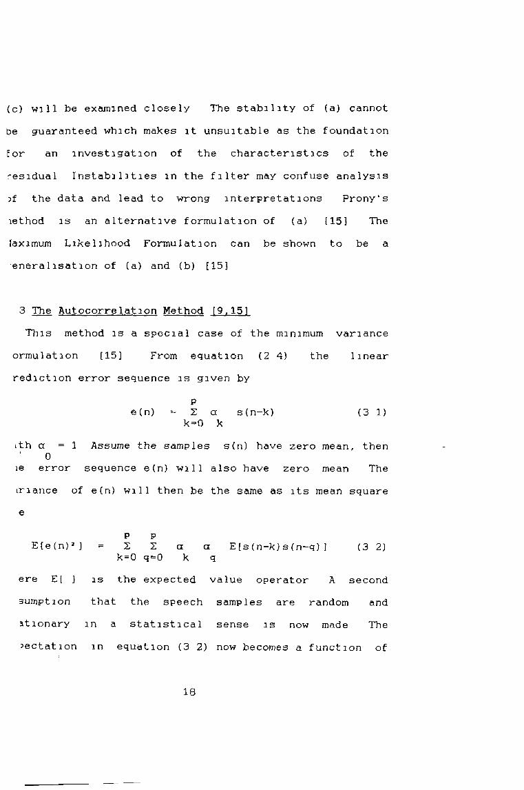
(c) will be examined closely The stability of (a) cannot be guaranteed which makes it unsuitable as the foundation for an investigation of the characteristics of the residual Instabilities in the filter may confuse analysis >f the data and lead to wrong interpretations Prony's lethod is an alternative formulation of (a) [15] Thelaximum Likelihood Formulation can be shown to be aeneralisation of (a) and (b) [15]

3 The Autocorrelation Method [9,15]This method is a special case of the minimum variance

ormulation [15] From equation (2 4) the linear rediction error sequence is given by

Pe(n) - 2 a s(n-k) (3 1)

k=Q kith a = 1 Assume the samples s(n) have zero mean, then

0le error sequence e(n) will also have zero mean The inance of e(n) will then be the same as its mean square e

P PE [e (n) 2 ] 2 2 a a E [s(n-k)s(n-q)] ( 3 2)

k = 0 q= 0 k qere E[ ] is the expected value operator A secondsumption that the speech samples are random andationary in a statistical sense is now made The^ectation in equation (3 2) now becomes a function of

18

the difference between k and q In terms of the autocorrelation R(n)

E[s(n-k)s(n-q)] = R(q-k) (3 3)If the process s(n) is further assumed to be ergodic then

1 N-lR(q-k) = lim --- 2 s(n-k)s(n-q) (3 4)

N- >c° N n=0The predictor error variance can then be written as

p PE [e (n) 2 ] 2 2 a R(q-k)a (3 5)

k—0 q~ 0 k qThe problem has now reduced to finding values for a ,

Jp which minimise this equation Since we only have a

finite set of values, equation (3 4) cannot be directlyevaluated If the samples are windowed using a finitelength window (eg a Hamming window [16)) then equation (3 4) can be directly computed If the window length is N then all the samples s(n) outside the window are equal to zero Therefore equation (3 4) reduces to

1 N+p-1R (P) * 2 s (n) s (n+p) (3 6 )

N n-0where p = |q-k[ ( 3 7 )

3 4 Solution to Autocorrelation MethodTo find the values of a , 1 = 1 p which minimise the

iprediction variance given in equation ( 3 5 ) , differentiate with respect to (w r t ) a , 1 = 1 p and set the result

l

19

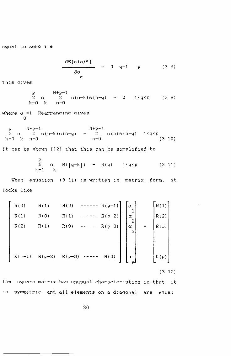
equal to zero 1 e

6 E [ e ( n ) 2 ]------------ - 0 q=l p (3 8 )

6 aq

This givesP N+p-12 a 2 s(n-k)s(n-q) = 0 liqlp (3 9)

k= 0 k n= 0

where a =1 Rearranging gives 0

P N+p-1 N+p-12 a 2 s(n-k)s(n-q) = 2 s(n)s(n-q) liqip

k=0 k n=0 n=0 (3 10)It can be shown [12] that this can be simplified to

P2 a R(lq-kl) = R (q) l<q<P (3 11)

k=l kWhen equation (3 1 1 ) is written m matrix form, it

looks like

R (0) R(l) R (2) --- -- R(p -1) a R(l)l

R (1) R(0 ) R (1) --- R(p-2 ) a R (2)2

R (2 ) R C1) R (0 ) --- — R(p-3) a = R(3)3

R(p-l) R(p-2 ) R (P-3) --- -- R (0 ) a R(p)- - - P- -

(3 12)r h e square matrix has unusual characteristics in that it is symmetric and all elements on a diagonal are equal

20

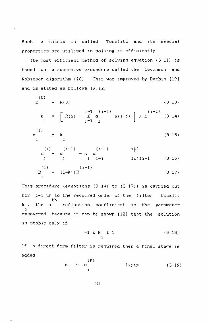
Such a matrix is called Toeplitz and its special properties are utilised in solving it efficiently

The most efficient method of solving equation (3 11) is based on a recursive procedure called the Levinson and Robinson algorithm [18] This was improved by Durbin [19] and is stated as follows [9,12]

(0)E « R (0) (3 13)

r i-l (i-l) -i (i-l)k = R ( i ) - 2 a Rd-j) / E (3 14)i L j-1 j J

(i)a * k (3 15)i l

( i ) d - 1 ) d - 1 ) i f la = a - k a

3 3 i i-j 1<j<i-1 (3 16)(i) (i-l)

E = (1-k2)E (3 17)l

This procedure (equations (3 14) to (3 17)) is carried outfor i=l up to the required order of the filter Usually

thk , the i reflection coefficient is the parameterl

recovered because it can be shown [1 2 ] that the solution is stable only if

-1 < k < 1 (3 18)l

If a direct form filter is required then a final stage is added

(P)ct = a lijip (3 19)J 3

21

where a is the direct form filter value J

In the calculation of the LPC parameters, it can be shown [15] that using infinite precision arithmetic guarantees the stability of the recursion

3 5 The Formulation and Solution of the Lattice Method

f (n) 0

f (n) 1

f (n) f (n) 2

f (n)

0 1 2 p - 1 p

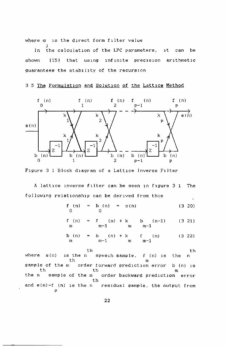
Figure 3 1 Block diagram of a Lattice Inverse Filter

A lattice inverse filter can be seen m figure 3 1 The following relationship can be derived from this

f (n) b (n) = s(n)0 0

f (n) = f (n) + k b (n-1 )m m-1 m m-1

b (n) = b (n) + k f (n)m m - 1 m m - 1

th

(3 20)

(3 21)

(3 22)

thwhere s(n) is the n speech sample, f (n) is the n

th msample of the m order forward prediction error b (n) is

th th mthe n sample of the m order backward prediction error

thand e(n)=f (n) is the n residual sample, the output from

P

22

th

Makhoul [1 0 ] derived several formulations based on thelattice filter by minimising some norm of the forwardresidual f (n) or backward residual b (n) or a combination

m mof both

To simplify derivations the following definitions are made

the p stage of the inverse filter

F (n) = E f2 (n) | (3 23)m L m

B (n) = E b2 (n) | (3 24)m L m

[f2 (n) 1L m J|"b2 (n) 1 L m J

C (n) = ETf (n) b (n-l)l (3 25)m L m m J

If the variance of the forward prediction error isminimised the following relationship can be derived

E[f (n) b (n-l)l C (n)f L m-l m - 1 J m - 1

k « - = - ( 3 260m r B (n-1)

m - 1Fb2 (n-1 ) 1 L m - 1 J

This result is equivalent to the autocorrelation method as it is also derived by minimising the mean square forward error

The backward method can be derived in a similar fashion except this time the variance of the backward prediction error is minimised [10] The following relationship holds

23

m

if (n) b (n-l)l L m - 1 m - 1 J

E[f2 (n) 1L m - 1 J

C (n) m - 1

F (n) m - 1

(3 27)

f bIt can also be shown [10] that the sign of k and k are

m midentical for all m

th f fMakhoul defined a generalised q mean of k and k as

sign(k )f q b q -,

I k | + | k |l / q

(3 28)

For k to be a reflection coefficient it must satisfy equation (3 18) This limits the value of q in the above to

q < 0 (3 29)A particular case which interests us is when q=-l This

is called the Harmonic Mean Method [10], Burg Method [17] or Maximum Entropy Method Inserting q=-l into equation (3 28) gives [10]

B - 1 k = k m

f b 2k k

f b k + k

2C (n) m - 1

(3 30)F (n) m - 1

B (n-1) m - 1

The recursion is carried out by combining equations (3 30) , (3 20) (3 21) and (3 22) and performing therecursion for m=l p, the required order of the filter

24

The lattice methods discussed do not perform a global :>timisation Instead a series of local optimisations are irned out, one as each order of the filter is ilculated Also, the addition of an extra filter order >es not affect those calculated in previous recursions When deriving the lattice formulations, Makhoul made no

¡sumption concerning the stationarity of the signal to be edicted However, he showed [10] that the lattice method sub-optimal if the signal is not stationary Only when e signal is stationary does the lattice method give the me solution as the autocorrelation method

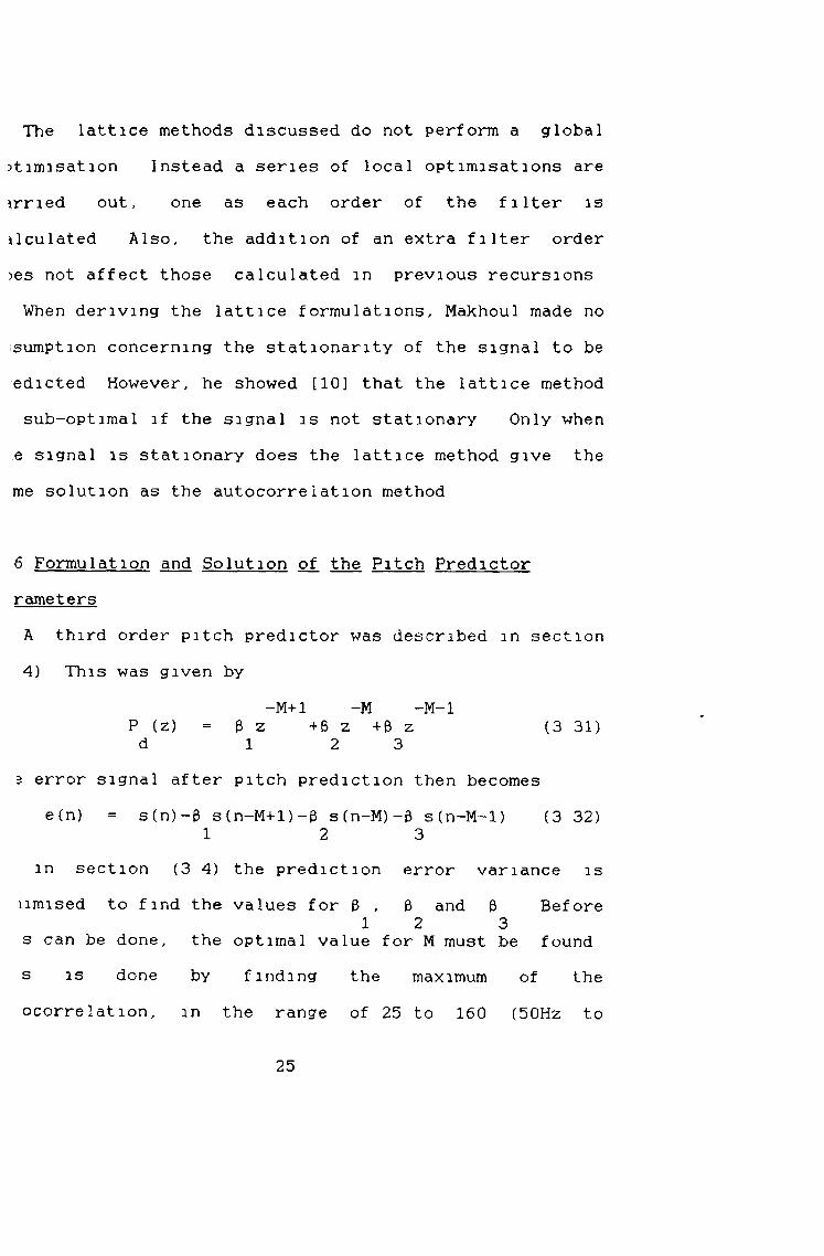
6 Formulation and Solution of the Pitch Predictor rametersA third order pitch predictor was described in section 4) This was given by

-M+l -M -M-l P (z) - 0 z +0 z +3 z (3 31)d 1 2 3

5 error signal after pitch prediction then becomese(n) = s(n)-0 s(n-M+l)-p s(n-M)-0 s(n-M-l) (3 32)

1 2 3in section (3 4) the prediction error variance is

limised to find the values for 3 , 3 and 0 Before1 2 3

s can be done, the optimal value for M must be founds is done by finding the maximum of theocorrelation, m the range of 25 to 160 (50Hz to

25

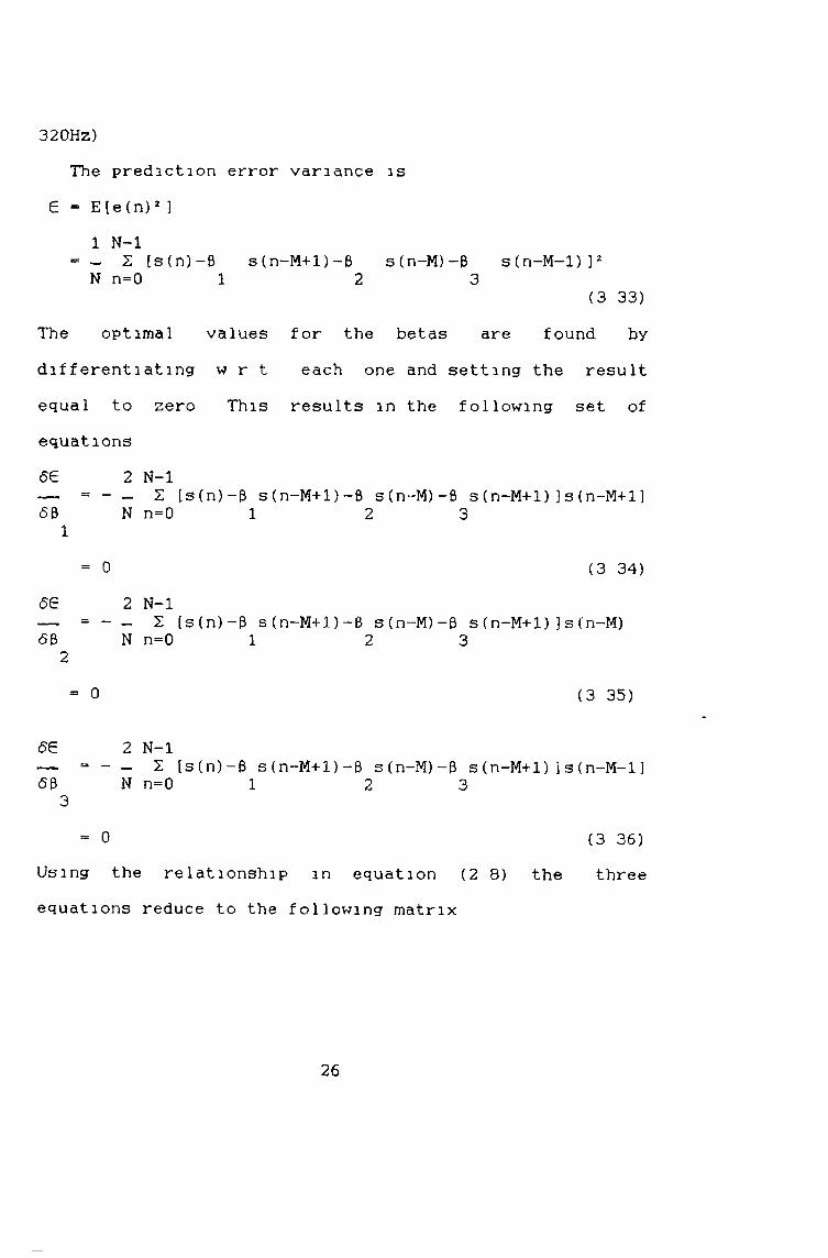
320Hz)The prediction error variance is

e = E [e (n) 2 ]1 N-l

= - 2 [s(n)-0 s(n-M+1)-B s(n-M)-0 s(n-M-l) ] 2N n=0 1 2 3

(3 33)The optimal values for the betas are found bydifferentiating w r t each one and setting the resultequal to zero This results in the following set ofequations 6 € 2 N-l— = - - 2 [s(n)-0 s(n-M+l)~0 s(n-M)-0 s(n-M+1))s(n-M+1]60 N n=0 1 2 3

1

- 0 (3 34)6 6 2 N-l— = - - 2 [s(n)-0 s (n-M+1)-0 s(n-M)-0 s(n-M+1))s(n-M)60 N n=0 1 2 3

2

” 0 (3 35)

6 6 2 N-l— - - - 2 [s(n) - 0 s(n-M+1)-0 s(n-M)-B s(n-M+1 )]s(n-M-1360 N n=0 1 2 3

3= 0 ( 3 36)

Using the relationship m equation (2 8 ) the threeequations reduce to the following matrix

26

< s2 > n-M+1

<s s > <s s >n-M+1 n~M n-M+1 n-M-1

<s s > <s2 >n-M+1 n-M n-M

<s s >n-M n-M-1

<s s > < s s > < s 2 >n-M+1 n-M-1 n-M n-M-1 n-M-1

01

02

03

< s >n-M+1

< s >n-M

< s >n-M-1

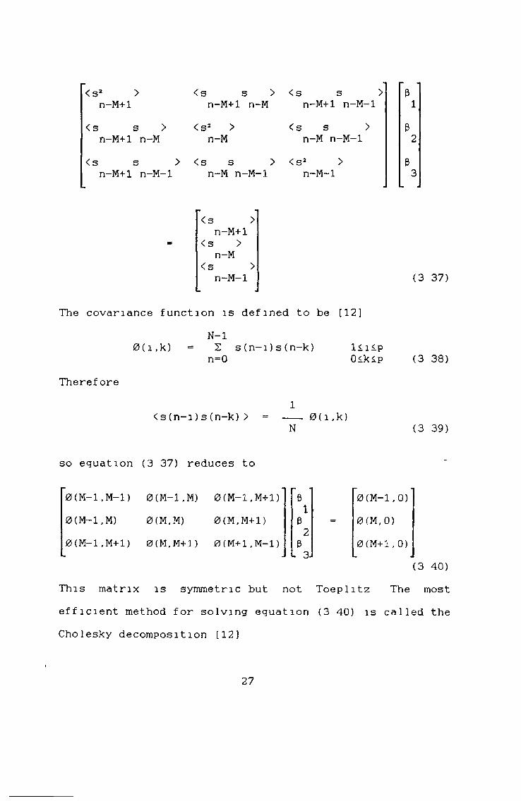
The covariance function is defined to be [12

0(i,k)N-l

2 s(n-i)s(n-k) n= 0

1< i<P 0 <k< p

Therefore

(3 37)

(3 38)

< s(n-i)s(n-k)> 0(i,k)N (3 39)

so equation (3 37) reduces to

0 (M-l, M-l) 0 (M-l,M) 0 (M-l,M+l) 0 0 (M-l,0 )0 (M-l, M) 0 (M, M) 0 (M,M+1)

10 = 0 (M, 0)

0 (M—1 ,M+l) 0 (M, M+l) 0 (M+l,M-l)Z

0 0 (M+l,0 )- . L 3-J . .(3 40)

This matrix is symmetric but not Toeplitz The most efficient method for solving equation (3 40) is called the Cholesky decomposition [123

27

If equation (3 40) is written as= 0

then the matrix $ can be expressed ast

$ = VDVwhere V is a lower triangular matrix (whose main elements are all 1), D is a diagonal matrix and transpose

It can be shown [12] that

V = [*0(i7 3 ) - V d V 1 / d 1<j<i-U L k=l ik k jk J 3

and the diagonal matrix is given byd - 0 (1 ,1 )1

i-ld = 0(i,i) - 2 V2 d i>2i k=l ik k

When the matrices D and V have been calculated,(3 41) can be rewritten as

tVDV O - 0

Def mingt

Y - DV n Insert this into (3 46) to get

VY = 6

-1Multiply across by D in equation(3 47) to get

(3 42) diagona1

denotes

(3 43)

(3 44)

(3 45)

equation

(3 46)

(3 47)

(3 48)

(3 41)

28

t - 1V n = D Y (3 49)

It has been shown [12] that equation (3 48) can beevaluated with

l-lY - 6 - 2 V Y p >i >2 (3 50)i i j-1 1J J

with initial conditionY = 0 (3 51)1 1

Finally equation (3 49) can be solved for O withP

f ï = Y / d ~ 2 V O l<i<p-l (3 52) l l i j = i + l j i j

with initial conditionO - Y / d (3 53)P P P

Note equation (3 52) is solved for i=p down to 1 = 1t

The general term for this solution is the covariance method [12] Unfortunately it is well known that the square matrix in equation (3 40) can become ill-conditioned This is because the covariance method is a restatement of Prony's method [15] and is attempting to model the signals by a series of exponentials Thisproblem is most prevalent in short frame analysis, wheregrowing sequences (the inclusion of a pitch pules) causethe solution to grow If the analysis frame is long (always greater than one pitch period) then such problems are reduced

29

If the matrix m equation (3 40) still becomes ill- conditioned, it can be re-conditloned by using the stabilised covariance method [20] This involves adding a constant to the main diagonal to ensure that all the eigenvalues are positive values

30

4 Implementation and Evaluation of LPC Analygig

4 1 IntroductionIn the previous chapter, two methods of producing

predictor parameters for a linear predictive analysis system were described In this chapter important characteristics of the autocorrelation and Burg methods will be compared using results derived from refereed literature These results will be used to select the method of analysis for the VXC system

Next the specific implementation details of the chosen method will be described Algorithms for pitch prediction and synthesis for both short and long term analysis will also be detailed

Finally, re-synthesis of the speech will be investigated and possible improvements to the traditional method of excitation of the LPC all-pole filter will be discussed

4 2 Specification of the LPC Ana lysis ParametersBefore a comparison of analysis methods can be carried

out, a specification for the type of analysis required must be drawn up This has to take into account the desire to improve on previous implementations

As stated in the introduction, one of the main areas of

31

degradation of current LPC algorithms is in plosives like /b/ Words like "fat" and "bat" analysed and synthesised using LPC tend to sound the same because the plosive changes into a fricative The reason for this is that the analysis interval used in the LPC is usually too long (20- 30ms) and this has the effect of smearing or averaging the plosive (a sudden burst of energy) Also as the plosive is a non-repetitive short duration pulse, it is not analysed properly by LPC algorithms which leave most of the plosive information m the residual signal [2 1 ]

In order to get around this problem, the analysis will be carried out using a 10ms analysis window The frame update rate will be 5ms and the sampling frequency will be 8kHz The speech will be low pass filtered to 3-4kHz prior to sampling to avoid aliasing This will give an analysis frame length of 80 with an update window length of 40

The speech is band limited to 3-4kHz by a high order filter, so some useful spectral information between 3-4kHz and 4kHz has been lost or severely attenuated In an attempt to recover some of this and improve analysis accuracy [93 the speech is pre-emphasised before analysis A filter of the form

-1F(z) =* 1-iiz (4 1 )

is used, where u is the pre-emphasis factor Typically a value of u - 0-9 is used

32

To make a logical decision on which LPC analysisalgorithm to choose, the two methods derived previuosly will be viewed under various headings below Both methods were implemented in a high level language so that information on storage requirements and computational cost could be determined These implementations also act as a benchmark for comparing with Finite Word Length (FWL) or assembler versions At this stage, steps were taken to implement both methods on a TMS32020 Digital Signal Processor so that FWL problems could be observed

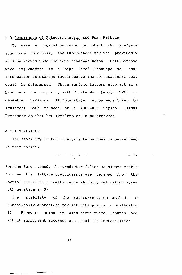
4 3 1 StabilityThe stability of both analysis techniques is guaranteed

if they satisfy-1 < k < 1 (4 2)

i

?or the Burg method, the predictor filter is always stable Decause the lattice coefficients are derived from the >artial correlation coefficients which by definition agree ath equation (4 2)

The stability of the autocorrelation method is heoretically guaranteed for infinite precision arithmetic 15] However using it with short frame lengths andithout sufficient accuracy can result in instabilities

4 3 Comparison of Autocorrelation and Burg Methods

33

In a recent paper [22] it was shown analytically thatthe Burg method gives superior results to theautocorrelation method under FWL The reason for this isbecause in the Burg method a local optimisation isperformed at each filter order The stages are thus

th"decoupled" and any error generated at the n- 1 stage

thwill be compensated for at the n stage

In the autocorrelation method, there is very strongth

coupling between stages Error generated at the n-1 stage are propagated and amplified in further stages Markel and Gray [15] investigated FWL effects in the autocorrelation method They conclude that in a FWL implementation of the autocorrelation method of LPC

(i) pre-emphasis should be applied as this gave a 3-4 bit improvement

(n) the sampling frequency should be as low aspossible

(in) the calculation of the autocorrelationcoefficients should be calculated usingmaximum precision and only the final resultshouId be rounded to the required word length

In particular they showed that at least 18 bits accuracy is required in an autocorrelation implementation so that only a negligible number of unstable filters will occur

4 3 2 Finite Word Length Effects

34

One of the assumptions in the autocorrelation formulation was that the waveform segment was zero outside the window of interest Therefore a time window must be used to effect this assumption A Hamming window [163 is used in the analysis of the speech The Hamming window is given by

h(n) - 0-54 - 0-46 cos (2irn/ (N-l)) 0<n<N-l0 Otherwise (4 3)

This has a superior performance to a rectangular window because it has a far higher attenuation m the stop band [16] and it also has a bandwidth twice that of a rectangular window A window is unnecessary in the Burg method as no assumptions were made about the signal outside the current area of interest

4 3 4 Computational Complexity and Storage RequirementsA summary of the data and computational requirements of

the two methods can be seen in table 4 1 All computation is measured in terms of multiply/adds because most current DSP chips are optimised around this type of calculation Taking into account the parameters arrived at in section (4 2), numerical values for storage needed and computational load are listed above These values do not include any overhead for control of the software as this

4 3 3 Tapered Time Windows

35

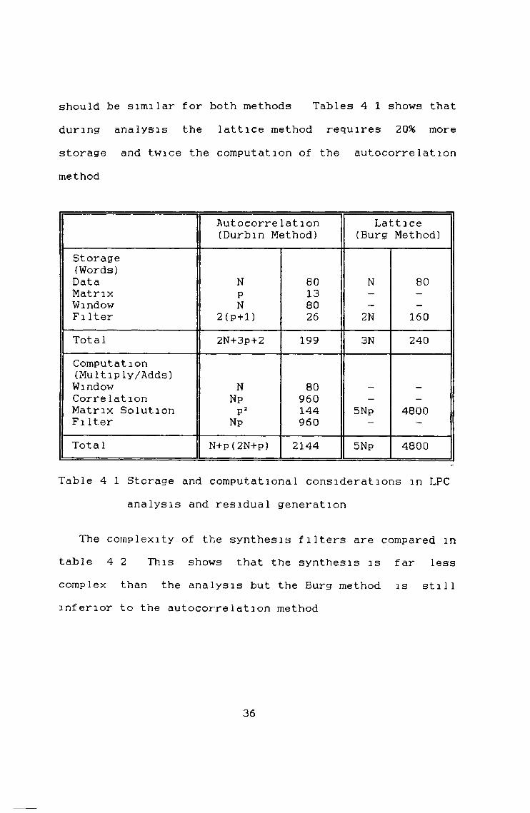
should be similar for both methods Tables 4 1 shows that during analysis the lattice method requires 2 0 % more storage and twice the computation of the autocorrelation method

Autocorrelation (Durbin Method)

Lattice (Burg Method)

Storage(Words)Data N 80 N 80Matrix P 13 - -Window N 80 - -Fi Iter 2 (p+l) 26 2N 160Total 2N+3P+2 199 3N 240Computation (Multiply/Adds)Window N 80 - —Correlation Np 960 - -Matrix Solution P2 144 5Np 4800Fi Iter Np 960 — —

Total N+p(2N+p) 2144 5Np 4800

Table 4 1 Storage and computational considerations in LPC analysis and residual generation

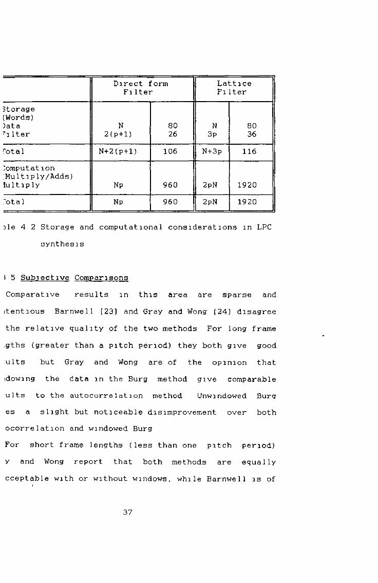
The complexity of the synthesis filters are compared in table 4 2 This shows that the synthesis is far less complex than the analysis but the Burg method is still inferior to the autocorrelation method

36

Direct form LatticeFilter FiIter

Storage(Words))ata N 80 N 807i Iter 2 (p+1 ) 26 3p 36Total N+2(p+1) 106 N+3p 116Computation;Multiply/Adds)lult ip ly Np 960 2pN 1920"ota 1 Np 960 2pN 1920

)le 4 2 Storage and computational considerations in LPC synthesis

* 5 Subjective ComparisonsComparative results in this area are sparse anditentious Barnwell [23] and Gray and Wong [24] disagree the relative quality of the two methods For long frame igths (greater than a pitch period) they both give good ults but Gray and Wong are of the opinion that idowing the data m the Burg method give comparable ults to the autocorrelation method Unwindowed Burg es a slight but noticeable disimprovement over both ocorrelation and windowed BurgFor short frame lengths (less than one pitch period) y and Wong report that both methods are equally cceptable with or without windows, while Barnwell is ofi

37

the opinion that no audible distortion occurs until the frame length is reduced below 60 (less than a pitch period in many cases)

In both these studies, no information was given about the type of speakers used (male/female) This makes a direct comparison difficult, but taking into account the stated frame length that will be used (80), both results show that the subjective advantage to be gained is at best marginal

4 3 6 DiscussionIn the examination of the various characteristics of

the two analysis methods, it is clear that they only differ strongly in one area computational complexity The autocorrelation method only has stability problems in fixed point implementation It has been shown however, that excellent results can be achieved with word lengths greater than 18-bits The processor to be used has a word length of 16-bits but it does support the restricted floating point format Q15 [25] and many fixed point calculations can be carried out to 32-bit precision

The spectral accuracy of the two methods for 80 sample frame lengths is marginal at best In some cases the Burg method gives better results [23], but perceptually the difference is small Gray and Wong [24] report improved

38

perceptual results with a windowed version of the Burg method It is noted that windowing would add further to the computational complexity of the Burg method

The computational load of the Burg method is extremely high, being twice as high as the autocorrelation method This large disparity could make the implementation of the proposed VXC system m real time very difficult Consequently, the autocorrelation method was chosen as the analysis method, as it offered reasonable results with low computational complexity and well documented instability problems which can be avoided

4 4 Implementation of the Autocorrelation Method of LPC Analysis

The effort required in implementing a real-time LPC analysis system (including pitch predictor) is extremely high The pressure this would put on resources woul'd detract from the investigation of the coder in the proposed VXC system Nevertheless , any implementation on a DSP, however inefficient, would be useful in demonstrating problems that wouId arise in rea 1 time systems thereby easing future development As an example, changes were made to the LPC software, implemented on the DSP, so that real time acquisition of speech could be accomp1ished The effect of this was to add a 10% overhead

39

in computation By the simple addition of a FIFO (first in, first out) buffer in hardware, the sampling could be reduced to a 1- 2 % overhead

The implementation used Q15 floating point format [25] instead of a fixed point implementation such as the LeRoux-Gueguen algorithm [26] This gives maximum analysis accuracy and is supported by the TMS32020 DSP used

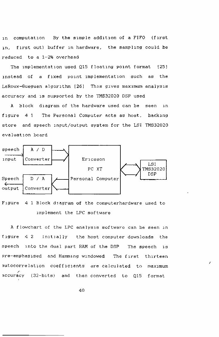
A block diagram of the hardware used can be seen in figure 4 1 The Personal Computer acts as host, backing store and speech input/output system for the LSI TMS32020 evaluation board

Figure 4 1 Block diagram of the computerhardware used to implement the LPC software

A flowchart of the LPC analysis software can be seen infigure 4 2 Initially the host computer downloads thespeech into the dual part RAM of the DSP The speech ispre-emphasised and Hamming windowed The first thirteenautocorrelation coefficients are calculated to maximum

saccuracy (32-bits) and then converted to Q15 formati

40

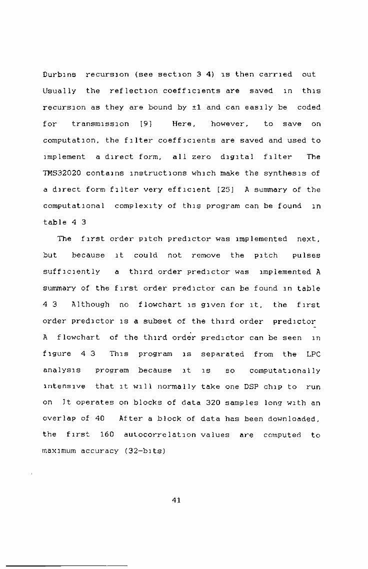
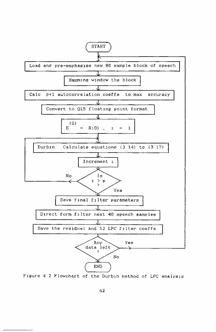
Durbins recursion (see section 3 4) is then carried out Usually the reflection coefficients are saved in this recursion as they are bound by ± 1 and can easily be coded for transmission [9] Here, however, to save on computation, the filter coefficients are saved and used to implement a direct form, all zero digital filter The TMS32020 contains instructions which make the synthesis of a direct form filter very efficient [25] A summary of the computational complexity of this program can be found in table 4 3

The first order pitch predictor was implemented next, but because it could not remove the pitch pulses sufficiently a third order predictor was implemented A summary of the first order predictor can be found in table 4 3 Although no flowchart is given for it, the firstorder predictor is a subset of the third order predictor

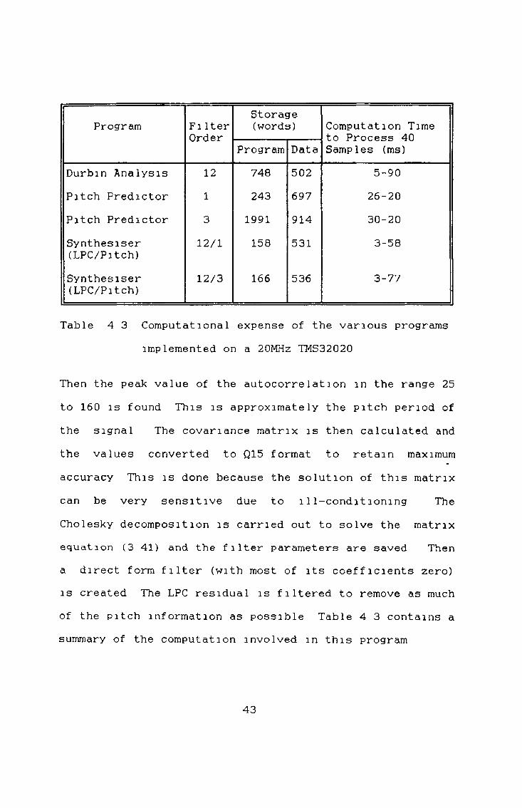
*A flowchart of the third order predictor can be seen m

figure 4 3 This program is separated from the LPC analysis program because it is so computationally intensive that it will normally take one DSP chip to run on It operates on blocks of data 320 samples long with an overlap of 40 After a block of data has been downloaded, the first 160 autocorrelation values are computed to maximum accuracy (32~bits)

41

42

Program Fi Iter Order

Storage(words) Computation Time

to Process 40 Samples (ms)Program Data

Durbin Analysis 1 2 748 502 CJl i o

Pitch Predictor 1 243 697 26-20Pitch Predictor 3 1991 914 30-20Synthesiser (LPC/Pitch)

1 2 / 1 158 531 3-58

Synthesiser (LPC/Pitch)

12/3 166 536 3-77

Table 4 3 Computational expense of the various programs implemented on a 20MHz TMS32020

Then the peak value of the autocorrelation in the range 25 to 160 is found This is approximately the pitch period of the signal The covariance matrix is then calculated and the values converted to Q15 format to retain maximum accuracy This is done because the solution of this matrix can be very sensitive due to ill-conditioning The Cholesky decomposition is carried out to solve the matrix equation (3 41) and the filter parameters are saved Then a direct form filter (with most of its coefficients zero) is created The LPC residual is filtered to remove as much of the pitch information as possible Table 4 3 contains a summary of the computation involved in this program

43

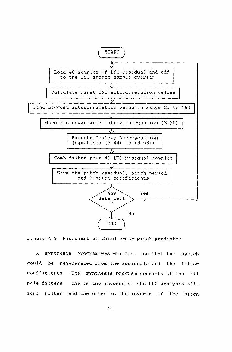
START

Load 40 samples of LPC residual and add to the 280 speech sample overlap

Calculate first 160 autocorrelation values

Find biggest autocorrelation value in range 25 to 160

Generate covariance matrix in equation (3 20)

Execute Cholsky Decomposition (equations (3 44) to (3 53))

Comb filter next 40 LPC residual samples

Save the pitch residual, pitch period and 3 pitch coefficients

Yes

Figure 4 3 Flowchart of third order pitch predictor

A synthesis program was written, so that the speech could be regenerated from the residuals and the filter coefficients The synthesis program consists of two all pole filters, one is the inverse of the LPC analysis all- zero filter and the other is the inverse of the pitch

44

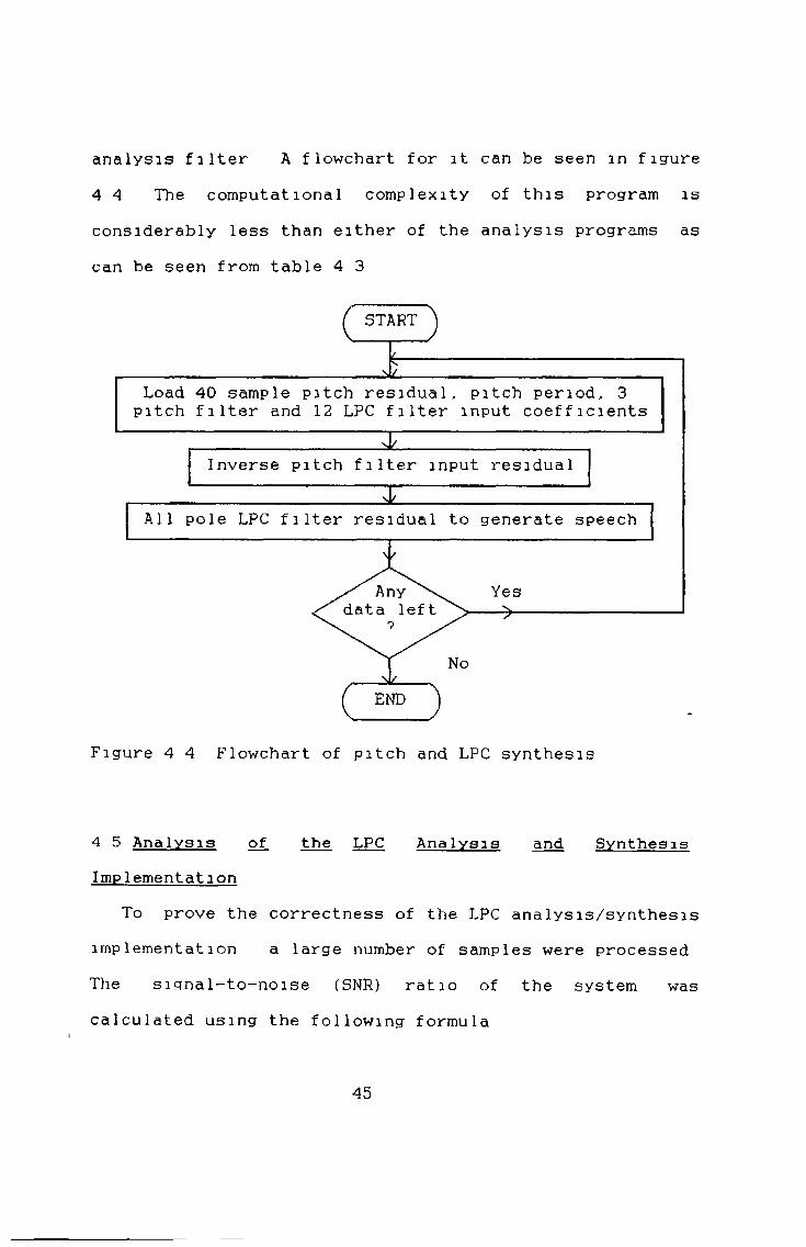
analysis filter A flowchart for it can be seen m figure 4 4 The computational complexity of this program is considerably less than either of the analysis programs as can be seen from table 4 3

4 5 Analysis of the LPC Ana lysis and Synthesis Implementation

To prove the correctness of the LPC analysis/synthesis implementation a large number of samples were processed The signal-to-noise (SNR) ratio of the system was calculated using the following formula

45

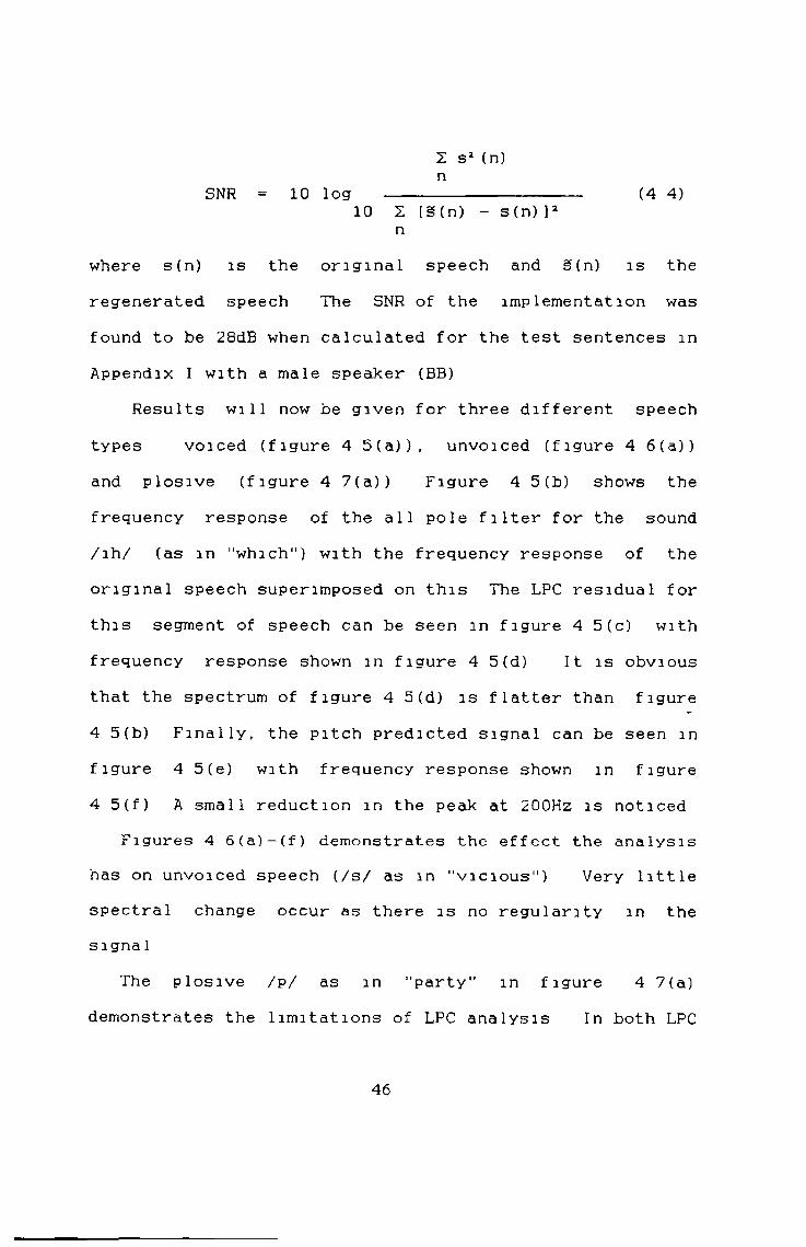
2 s2 (n) n

SNR = 10 log -------------------- (4 4)1 0 2 [S(n) - s(n ) ] 2

nwhere s(n) is the original speech and §(n) is theregenerated speech The SNR of the implementation wasfound to be 28dB when calculated for the test sentences in Appendix I with a male speaker (BB)

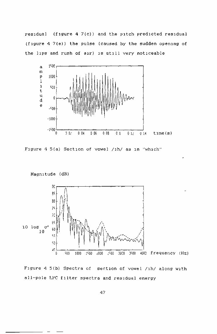
Results will now be given for three different speech types voiced (figure 4 5(a)), unvoiced (figure 4 6 (a)) and plosive (figure 4 7(a)) Figure 4 5(b) shows thefrequency response of the all pole filter for the sound /ih/ (as in "which") with the frequency response of theoriginal speech superimposed on this The LPC residual for this segment of speech can be seen in figure 4 5(c) with frequency response shown in figure 4 5(d) It is obvious that the spectrum of figure 4 5(d) is flatter than figure 4 5(b) Finally, the pitch predicted signal can be seen in figure 4 5(e) with frequency response shown in figure 4 5(f) A small reduction in the peak at 200Hz is noticed

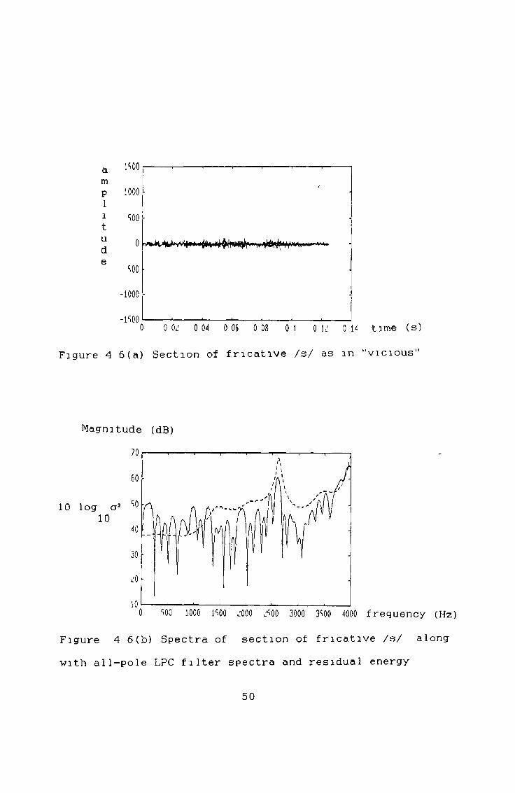
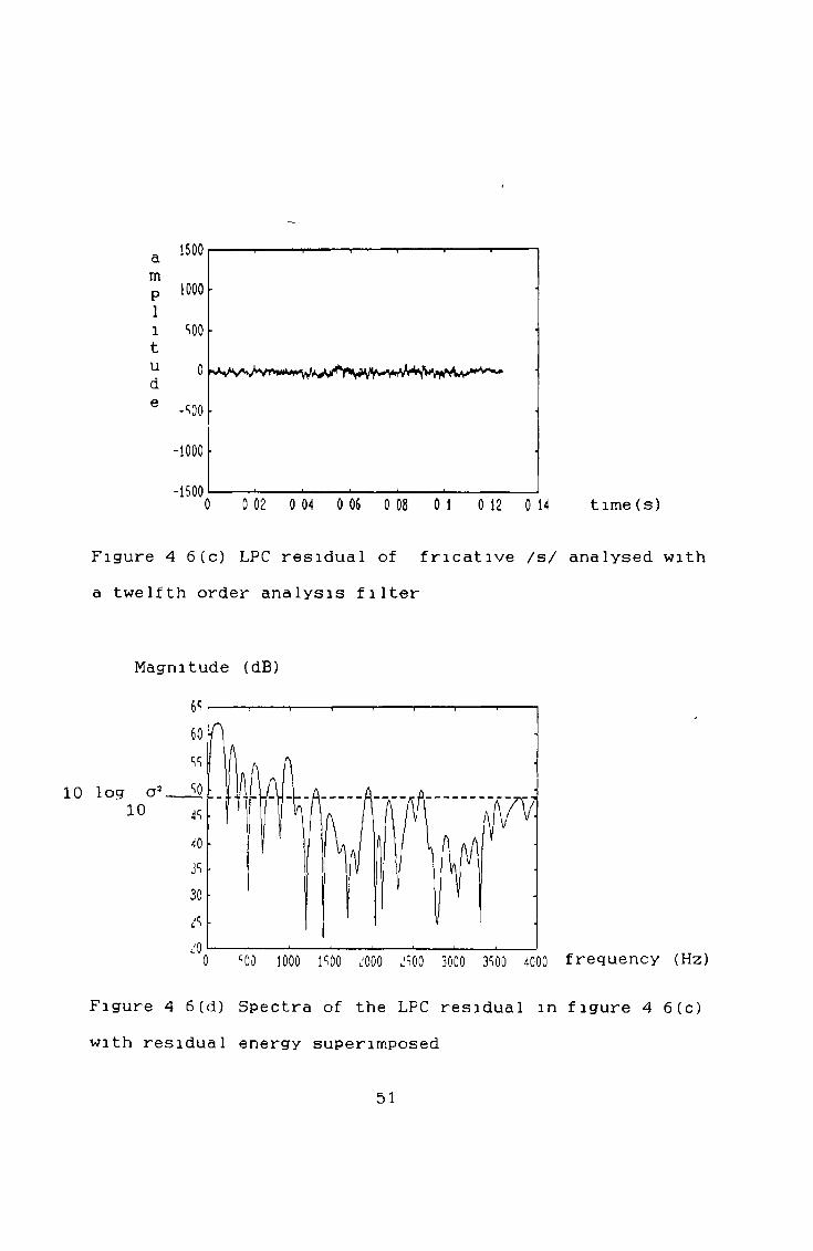
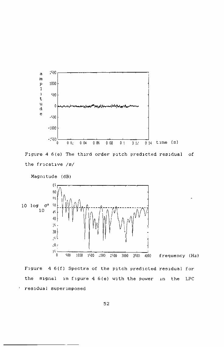
Figures 4 6 (a)— (f) demonstrates the effect the analysis has on unvoiced speech (/s/ as in "vicious") Very little spectral change occur as there is no regularity in thesigna 1

The plosive / p / as in "party" in figure 4 7(a) demonstrates the limitations of LPC analysis In both LPC

46

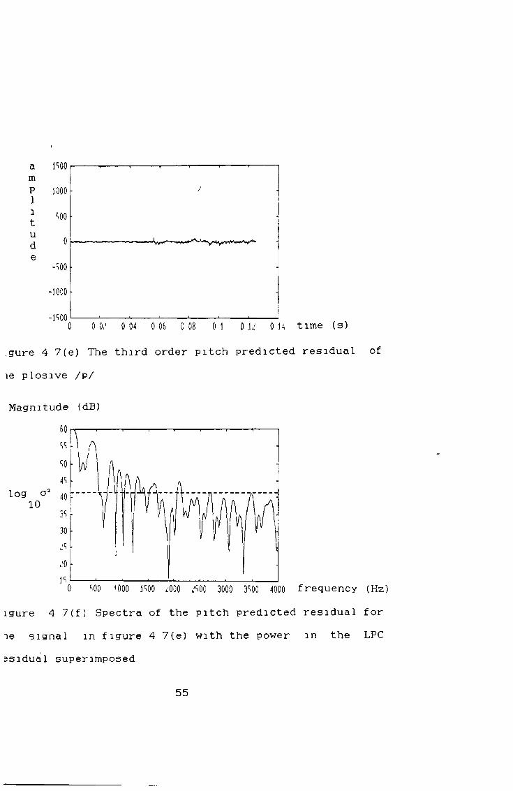
residual (figure 4 7(c)) and the pitch predicted residual (figure 4 7(e)) the pulse (caused by the sudden opening of the lips and rush of air) is still very noticeable

m

1000

soo

o

-soo

■1000

^000 0 0.' 0 04 0 06 0 08 0 1 0 \ i U 14 time(s)

Figure 4 5(a) Section of vowel /ih/ as in “which“

Magnitude (dB)

1 0 log a2 10

Figure 4 5(b) Spectra of section of vowel /ih/ along with all-pole LPC filter spectra and residual energy

47

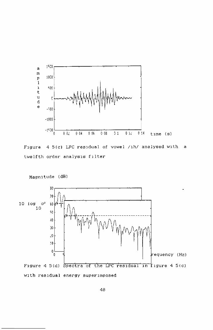
Figure 4 5(c) LPC residual of vowel /ih/ analysed with a twelfth order analysis filter

Magnitude (dB)

8070

1 0 log a2 60 1 0 SO

4030.'0300

0 S00 1000 1SOO ¿000 JSOO 3000 3SOO 4000 frequency (Hz)

Figure 4 5(d) Spectra of the LPC residual in figure 4 5(c) with residual energy superimposed

(dB)

48

Figure 4 5(e) The third order pitch predicted residual of the vowel /ih/Magnitude (dB)

1 0 log a2 10

0 f0) 1000 5^00 ,'000 , c00 JuOO 3W» 1000 frequency (Hz)

Figure 4 5(f) Spectra of the pitch predicted residual for the signal in figure 4 5(e) with the power in the LPC residual superimposed

49

amP11tude

1S00

1000

-1000

■isoo0 0 OJ 0 04 0 06 0 08 0 1 0 1,' 0 14 time (s)

Figure 4 6 (a) Section of fricative /s/ as m "vicious"

Magnitude (dB)70

60

1 0 log a2 ^10

40

30 .'0

100 SQ0 1000 1S00 ¿000 JS00 3000 3S00 4000 frequency (Hz)

Figure 4 6 (b) Spectra of section of fricative /s/ along with all-pole LPC filter spectra and residual energy

50

a 1500 mp 1000 1l S00tu 0de -SOO

-1000

-1500 0 0 02 0 04 0 06 0 08 0 1 0 12 0 14 t i m e ( s )

Figure 4 6 (c) LPC residual of fricative /s/ analysed with a twelfth order analysis filter

Magnitude (dB)6S 60 ss

1 0 log a2-__10 4S

40 JS 30 ¿S ¿00 SOO 1000 isoo ¿000 l'SOO 3000 3̂00 4000 frequency (Hz)

Figure 4 6 (d) Spectra of the LPC residual in figure 4 6 (c) with residual energy superimposed

51

mP 100011 SOOt

S 1

e -soo-1000

* ^0 0 0; 0 04 0 06 0 08 0 1 0 1.' 0 14 time (s)

Figure 4 6 (e) The third order pitch predicted residual of the fricative /s/

Magnitude (dB)6S 60 SS

1 0 log a2 SO 10 ^

40 3S 30 ,'S ¿0 IS0 soo 1000 1S00 ¿000 l'SOO 3000 3SOO 4000 frequency (Hz)

Figure 4 6 (f) Spectra of the pitch predicted residual for the signal in figure 4 6 (e) with the power in the LPC

1 residual superimposed

52

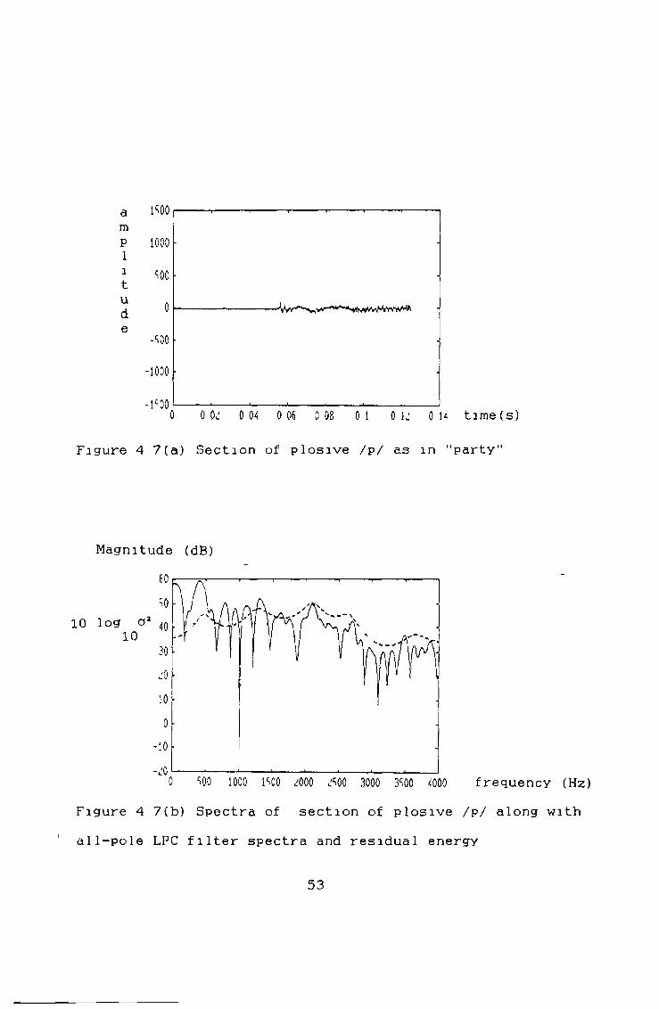
Figure 4 7(a) Section of plosive /p/ as m MpartyM

Magnitude (dB)60 SO

1 0 log a2 40 1 0

30 ¿0 10

0 >10

-¿00 soo 1000 isoo ¿000 ¿S00 3000 3S00 4000 frequency (Hz)

Figure 4 7(b) Spectra of section of plosive /p/ along with all-pole LPC filter spectra and residual energy

53

amP11tude

Figure 4 7(c) LPC residual of plosive /p/ analysed with a twelfth order analysis filter

Magnitude (dB)

1 0 log & 1 0

<¡00 3000 3S0G 4000 frequency (Hz)

Figure 4 7(d) Spectra of the LPC residual in figure 4 7(c) with residual energy superimposed

54

a mmP 10001i sootud 0

e -SOO

-1000

-1*5000 0 0,' 0 04 0 06 0 08 0 1 0 LJ 0 14 time (s)

.gure 4 7(e) The third order pitch predicted residual of le plosive /p/

Magnitude (dB)

log o ' 10

0 c.00 1000 1S00 ¿000 ¿soo 3000 3̂00 4000 frequency (Hz)igure 4 7(f) Spectra of the pitch predicted residual for ie signal in figure 4 7(e) with the power in the LPC ssidual superimposed

55

The analysis thus produces three different types of residual

(i) Residuals, derived from voiced speech, havinga high energy content and still retaining some pitch information and hence slight penodicy

(I I ) Noise like residuals with low energy derived from unvoiced speech

(I I I ) Residuals from plosive sounds, having a burst of energy relatively large compared with the preceding signal

4 6 Improving the Excitation of the LPC SynthesiserSo far a method has been described which optimally

matches the spectrum of short segments of speech with adigital filter The original speech was sampled at 8kHzwith a resolution of 1 2 -bits giving a transmission rateover a digital channel of 96k bits per second If instead, the filter parameters are transmitted, a much lower bit rate can be accomplished Several ways of encoding the filter parameters have been described m literature [1 1 ] showing that 1 2 filter parameters can be quantised to atotal of 40 bits (using fewer bits for higher orders) without much audible distortion With a frame update rate of Sms, this implies a bit rate of 8 k bits per second

56

Pitch period

Figure 4 7 Simplified model of speech production assuming purely voiced or unvoiced speech exists

In addition to transmitting the filter parameters, some information has to be sent about the excitation of the filter In traditional systems [ 1 2 ] , this information consists of a voiced/unvoiced (V/UV) decision, and when voicing was detected the pitch period was transmitted Furthermore the g a m of the residual was transmitted, so that the speech power of the encoder and decoder were matched This results in the system shown m figure 4 8 , with the all-pole filter being driven by either a white noise source (UV) or a periodic train of pulses (V) The information on voicing, pitch, gain and synchronisation typically took a further 13 bits per frame giving a total bit rate of 10600 bits per second Although this is a

57

considerable bit rate reduction (9 1), the quality of this is a best described as 'synthetic-qua1 ity1 having a robot like sound Further bit rate reductions are possible [27] and have bit rates of only 2400 bits per second, achieved using a 2 2 Sms frame

The major problem with the traditional LPC vocoder is in the excitation signal The pulse excitation has been shown to give good results for vowels and the noise source gives good results for pure fricatives However one with a combination of voiced and unvoiced sounds (e g /v/ as in "veal") or plosive sounds are very poorly represented To overcome this problem, many alternative driving signals have been used multi-pulse excitation [3], stocastic excitation only [4], coded residual [28] and various combinations of excitations [2 1 ]

The most promising of these m terms of bit rate reduction is Code Excited Linear Prediction (CELP) [4] The principle is to obtain a large sequence of the LP*C residual or (Gaussian noise), break this into vectors of fixed length and place them together into a codebook by averaging all those that have similar characteristics This codebook generation is computationally intensive, but is carried out "off-line" and it only has to be done once The encoding process finds the closest match for the generated residual within the codebook The position

58

within the codebook is transmitted to the decoder and the code is used to excite the synthesiser The efficient coding of the LPC parameters and residual will now be considered so as to preserve the reproduction accuracy over a wide range of different sounds

59

f

5 1 IntroductionIn the previous chapter , a specification of a speech

coding system was drawn up It requires the transmission of two filters, one representing short time spectral shape, the other containing pitch information This chapter will introduce a method whereby a group or block of parameters are quantised A review of the methods currently in use is included, along with the most popular algorithm A method for reducing the transmission rate of the LPC parameters will be outlined

5 2 Pre1iminariesA vector quantiser was defined by Gray [28] as

“a system for mapping a sequence of continuous or discrete vectors into a digital sequence suitable for communication over or storage in a digital channe1 ”

The objective in this mapping is the reduction of the bit rate This is accomplished by assigning a symbol to a vector at an encoder the transmission of the symbol over a channel and reconstruct ion of a vector at the decoder It is clear that a large saving in bit rate could be attained if a vector (of arbitrary length) is represented

5 Vector Quantisation

60

by one symbolThis conversion of high rate data into low rate data

inevitably involves a loss of fidelity Consequently the problem faced in designing a vector quantisation system is, given a fixed bit rate B, obtain the lowest possible distortion or alternatively minimise the bit rate for a given fidelity The objective therefore, is to generate an ensemble of vectors, called a codebook, which best represents all possible types of vectors

5 3 Formulation of the Codebook Design ProblemThe LPC system described previously gives out an N (=40

in our system) sample residual every iteration In vectorquantisation, each N sample residual vector, x, is mappedonto another vector y of the same length under thetransformation

y = Q(x) (5 1)The input vector, x, can take on a large (possibly infinite) number of states, while output vector, y, can only take on L states (known as the number of codebook levels) The quantisation operation, Q( ) assigns to y the vector in the codebook, C, which is the least cost approximation of x To design the codebook, C, the N- dimensional space has to be divided into L cells (which adequately span all possible inputs x) and each cell C ,

l

61

liiiL, is assigned a vector yl

The assignment of vector y as the quantised version ofvector x entails a cost known as the distortion A measureof this difference is usually written d(x,y), the measureof dissimilarity of the two vectors

In a codebook of length LB = log L bits (5 2)

2are needed to code each vector The transmission rate is

T = BF bits/s (5 3)T

where F is the number of codewords transmitted per T

second The rate per dimension (useful when talking about vectors) is

BR = --- bits/dimension (5 4)

N

5 4 Motivation for Using Vector QuantisationRate distortion theory is the branch of information

theory devoted to data compression This theory was developed by Shannon [29,30] and further elaborated upon by Gallagher [31] and Berger [32] Using it, the upper and lower bounds of performance of data compression systems can be theoretically determined The Rate DistortionFunction, R(D), is defined as the smallest value of the rate per dimension, R attainable for a fixed distortion,

62

o

D The inverse of this is the Distortion Rate Function D(R) It is the minimum distortion, D that can be achieved at a fixed rate, R

It can be shown [33] that the upper bound on D(R) for a memoryless Gaussian source with variance a2 , is given by

-2RD (R) = 2 a2 (5 5)G

For the transformation m equation (5 1) the averagedistortion in quantising x as y is given by

D = E [d (x, y) ] (5 6 )where d(x,y) is the distortion per dimension It can beshown [32] that the minimum distortion rate D (R) for a

Nfixed rate R is

D (R) = min E[d(x,y)] (5 7)N Q(x)

where the minimum is found over all possible mappings ofQ(x) The lower bound is found in the limit as N->®, i e

*D (R) - lim D (R) (5 8 )

N- >oo NThis demonstrates the fundamental result of rate

distortion theory coding of vectors will always produce better results than with scalars and in theory, one can approach the distort ion rate function arbitrarily c lose by increasing the vector dimension N

63

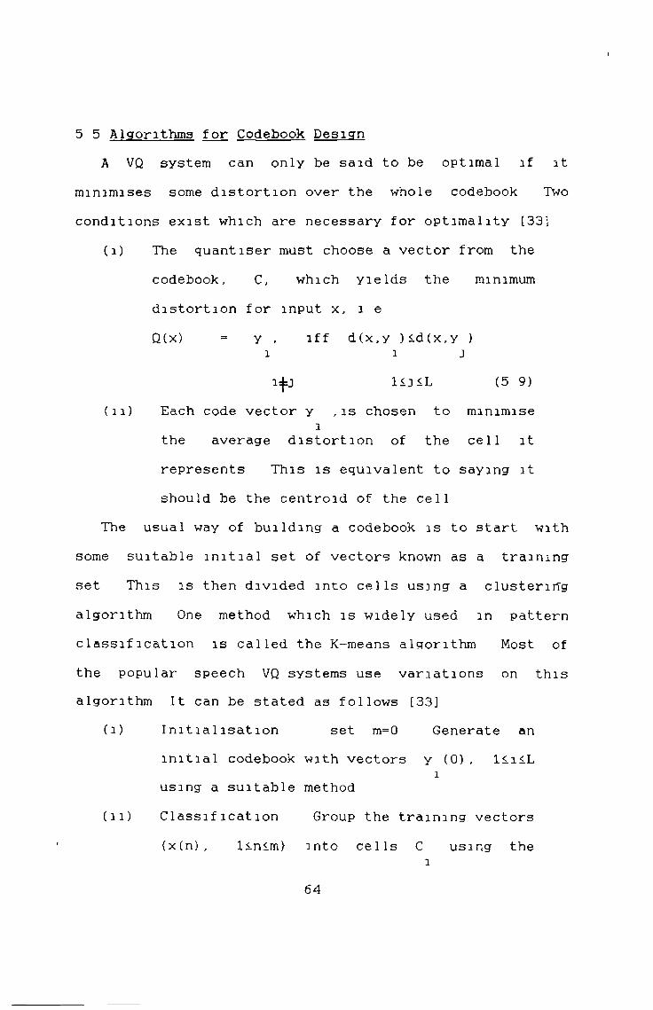
A VQ system can only be said to be optimal if it minimises some distortion over the whole codebook Two conditions exist which are necessary for optimality [33]

(I) The quantiser must choose a vector from thecodebook, C, which yields the minimumdistortion for input x, i eQ(x) « y , iff d(x,y )<d(x,y )

i i 3

i$ 3 1<J<L (5 9)(n) Each code vector y , is chosen to minimise

ithe average distortion of the cell itrepresents This is equivalent to saying itshould be the centroid of the cell

The usual way of building a codebook is to start withsome suitable initial set of vectors known as a trainingset This is then divided into cells using a clusteringalgorithm One method which is widely used in patternclassification is called the K-means algorithm Most ofthe popular speech VQ systems use variations on thisalgorithm It can be stated as follows [33]

(i) Initialisation set m=0 Generate aninitial codebook with vectors y (0), l<i<L

iusing a suitable method

(I I ) Classification Group the training vectors {x(n), linim} into cells C using the

i

5 5 Algorithms for Codebook Design

64

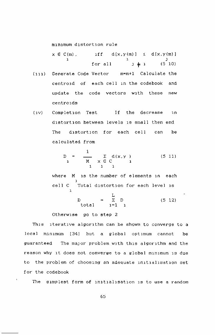
x € C(m), iff d[x,y(m)] < d[x,y(m)]1 i J

for all j 1 (5 10)( m ) Generate Code Vector m=m+l Caleu 1 ate the

centroid of each cel 1 m the codebook andupdate the code vectors with these newcentroids

(iv) Comp letion Test If the decrease indistortion between levels is small then end The distortion for each cel 1 can be calculated from

1D = 2 d(x,y ) (5 11)i M x E C l

i l l

where M is the number of elements in eachi

cell C Total distortion for each level isl

LD = 2 D (5 12)total 1 = 1 l

Otherwise go to step 2This iterative algorithm can be shown to converge to a

loca1 minimum [34] but a globa1 optimum cannot beguaranteed The major problem with this algorithm and thereason why it does not converge to a global minimum is dueto the problem of choosing an adequate initialisation setfor the codebook

The simplest form of initialisation is to use a random

minimum distortion rule

65

training sequence for the first L codes or a piece of data from the signal to be coded A second form of initialisation is to apply a scalar quantiser many times in succession and then cut down the vector codebook to the required size [35] A third type of initialisation uses the "splitting" technique [34,36) This starts by finding the centroid of a small sequence This centroid is perturbed to form two new centroids The K-means algorithm is then run to find the optimum 1 -bit quantiser for this training sequence This procedure is carried out until the desired rate of the codebook is reached

Variations on the K-means algorithm have been discussed widely in literature (see Gray [28] for a summary) Most of these are sub-optimal in a coding sense as they attempt to reduce computational complexity and/or memory requirements through the use of alternative searching strategies to full search However, they do achieve results approaching those of the optimal VQ system

5 6 Vector Quantisation of the LPC ParametersThis section describes a method by which the LPC voice

coder can be compressed using VQ techniques A major problem in coding LPC parameters is finding a suitable distortion measure The Itakura-Saito distortion measure [37] has been shown to be analytically tractable,

66

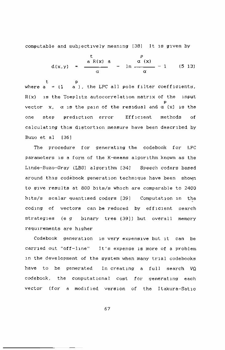
computable and subjectively meaning [38] It is given byt P

a R(x) a a (x)d(x,y) - - In ------- - 1 (5 13)

a at p

where a - (1 a ), the LPC all pole filter coefficients,R(x) is the Toeplitz autocorrelation matrix of the input

pvector x, a is the gain of the residual and a (x) is the one step prediction error Efficient methods of calculating this distortion measure have been described by Buzo et al [36]

The procedure for generating the codebook for LPCparameters is a form of the K-means algorithm known as the Lmde-Buzo-Gray (LBG) algorithm [34] Speech coders based around this codebook generation technique have been shov^n to give results at 800 bits/s which are comparable to 2400bits/s scalar quantised coders [39] Computation in thecoding of vectors can be reduced by efficient searchstrategies (e g binary tree [39]) but overall memory requirements are higher

Codebook generation is very expensive but it can be carried out "off-line" It's expense is more of a problem in the development of the system when many trial codebooks have to be generated In creating a full search VQ codebook, the computational cost for generating each vector (for a modified version of the Itakura-Sat1 0

67

distortion) is [33]

By definition, each vector is coded using B=RN=log L bits2

ThereforeRN

C = N2 (5 15)If a training sequence of length M is used and Iiterations are required, then the total cost is

RNC = IMN2 (5 16)T

Therefore the computational costs grow exponentially with vector length and rate per dimension It can also be shown that total memory cost is

RNM = N (2 + M) (5 17)T

Lack of large computational resources usually hampers research in this area The subject of interest is the coding of the residual, so construction of a VQ system for the LPC was avoided as this would spread available resources too thinly Nevertheless it would be possible to code the LPC system described in section (4 4) a 2400 bits/s with little additional extra distortion

C « NL (5 14)

68

6 Algorithms for Waveform Vector Quantisation

6 1 IntroductionThe LBG algorithm will be applied to waveform coding of

the LPC Residual The limitations of the algorithm will then be discussed An alternative approach proposed by Equitz [5] called the Pairwise Nearest Neighbour (PNN) algorithm will be described It will be demonstrated that it gives comparable results at a lower computational cost and goes some way to improving upon the shortcomings of the LBG algorithm

6 2 Waveform Vector QuantisationThe basic technique of VQ could be directly applied to

speech by creating a codebook using a version of the K- means algorithm However because of the amount of information in the speech signal, a large codebook of small dimension vectors would be required to give good results Reducing the bit rate in such a system would require an increase in vector length to keep the distortion sma1 1 It has been shown that this causes an exponential increase in resources (equations (5 15) and (5 16)) Also problems arise due to "edge effects" because when codes are joined together discontinuities occur causing distortion

69

A way of removing a large amount of information in speech using LPC has already been described, so it makes sense to assume that far fewer codes should be needed to represent the LPC residual Figures (4 4(e)), (4 5(e)) and

‘ (4 6 (e)) have shown that the waveform becomes fairly random after short and long term spectral information has been removed

If each sample of the residual is coded independently (i e scalar quantisation), then between 8 bits (using Pulse Coded Modulation (PCM)) and 3 bits (using Adaptive Differential PCM) would be required to adequately code it [8 ] This results in a rate of between 74k bits per second and 32k bits per second when spectral information is included Although it is well known that such systems give high quality speech, the bit rate reduction is small and transmission over telephone bandwidth lines is not possible

Schroeder and Atal [4] proposed the use of a purely random Guassian innovation as excitation source at the decoder called Code Excitation Linear Prediction or CELP The results, although promising showed that massive computation was needed (~ 3200 million multiply/adds per second) because a 1 0 -bit full search codebook was required The signa1-to-noise ratio of this system was always poor in the region of rapidly changing speech

70

power An alternative excitation is to use vectors based upon the residual of the LPC system This is usually referred to as Vector Excitation Coding or VXC

LPC coding gives three sets of parameters spectral filter, pitch filter and gain, which can be coded using VQ to reduce the bit rate The separate coding of LPC parameters and residual is known as a product code and can achieve better results overall if each step is independent It has been argued by Makhoul [33] that such is the case for the LPC, pitch, gain and residual coding stages Therefore separate codebooks can be created with only a small performance degradation over using one large codebook Furthermore, it would be difficult to find a distortion measure which would adequately cover all stages meaningfully and enable optimal joint quantisation

In CELP, the residual is quantised as part of the analysis procedure, 1 e the residual code is chosen as the one which minimises the distortion of the input speech Although better results can be achieved than by directly comparing residuals, the computational cost is prohibitive Within CELP, the most expensive task is the re-synthesis of each vector in the codebook, so that synthetic speech can be compared with original speech

71

*

LPC Pitch NormalisedResidual Residual Residual

Figure 6 1 A block diagram of an LPC waveform coding system

A shortcut that saves 90% of the computation, is tocompare the residual generated during analysis with allvectors in the codebook A block diagram for this type ofwaveform coding system can be seen in figure ( 6 1 ) TheLPC and pitch predictor parameters are calculated in thenormal way The gain of the residual is then found andused to normalise it so that only a "shape" vectorremains The gain can now be quantised separately Adistortion measure is used to find the closest code vectorto the input residual vector

The distortion measure used m waveform coding isusually the Mean Square Error (MSE) or L norm given by

2N—1

d(x ,y) - ||x"y|i2 = 2 (x - Y)2 (6 1 )1 = 0

where N is the vector length Although the squared error gives a useful measure of the similarity of the shape of

72

vectors, it lacks perceptual meaning when applied to speech Being among the few tractable measures available, it will be used for the present The performance of this type of coder is usually measured in terms of signal-to- noise-ratio

The calculation of the best code for transmission can be very expensive if the codebook is long, because no shortcut m calculation of the distortion measure can be made Therefore code length and codebook size should be kept to a minimum

6 3 Analysis of a Waveform VQ System using the LBG Algorithm

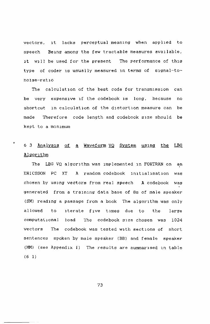
The LBG VQ algorithm was implemented m FORTRAN on an ERICSSON PC XT A random codebook initialisation was chosen by using vectors from real speech A codebook was generated from a training data base of 8 s of male speaker (SM) reading a passage from a book The algorithm was only allowed to iterate five times due to the large computational load The codebook size chosen was 1024 vectors The codebook was tested with sections of short sentences spoken by male speaker (BB) and female speaker (MM) (see Appendix I) The results are summarised in table (6 1)

73

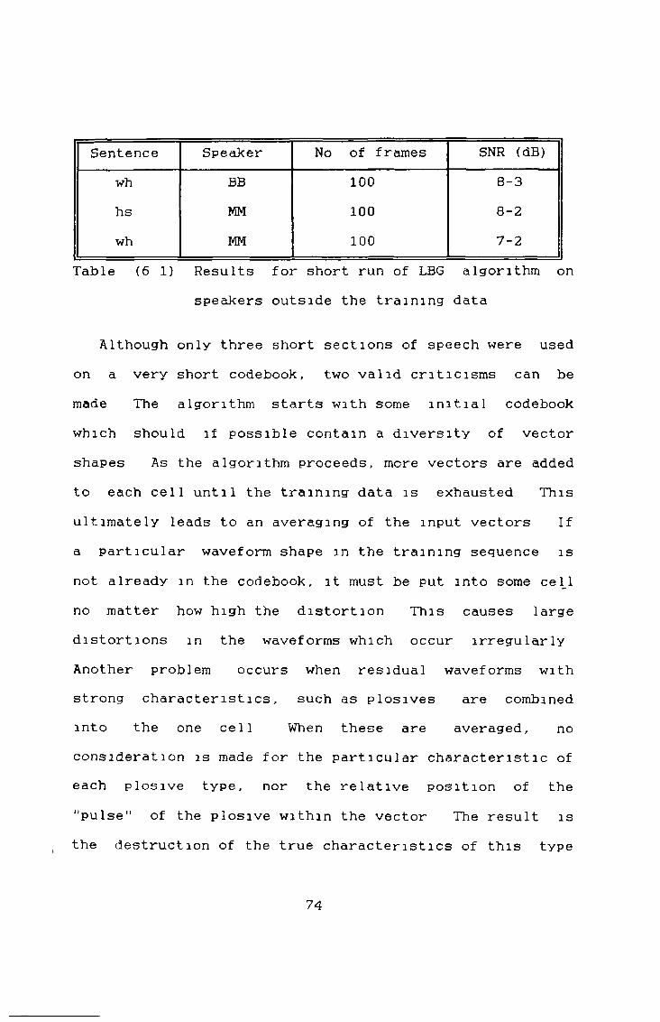
Sentence Speaker No of frames SNR (dB)wh BB 1 0 0 8-3hs MM 1 0 0 8 - 2

wh MM 1 0 0 7-2Table ( 6 1) Results for short run of LBG algorithm on

speakers outside the training data

Although only three short sections of speech were used on a very short codebook, two valid criticisms can be made The algorithm starts with some initial codebookwhich should if possible contain a diversity of vector shapes As the algorithm proceeds, more vectors are added to each cell until the training data is exhausted This ultimately leads to an averaging of the input vectors If a particular waveform shape in the training sequence is not already in the codebook, it must be put into some cell no matter how high the distortion This causes large distortions in the waveforms which occur irregularly Another problem occurs when residual waveforms with strong characteristics, such as plosives are combined into the one cell When these are averaged, noconsideration is made for the particular characteristic ofeach plosive type, nor the relative position of the "pulse" of the plosive within the vector The result is the destruction of the true characteristi c s of this type

74

of signal

¿WO sample

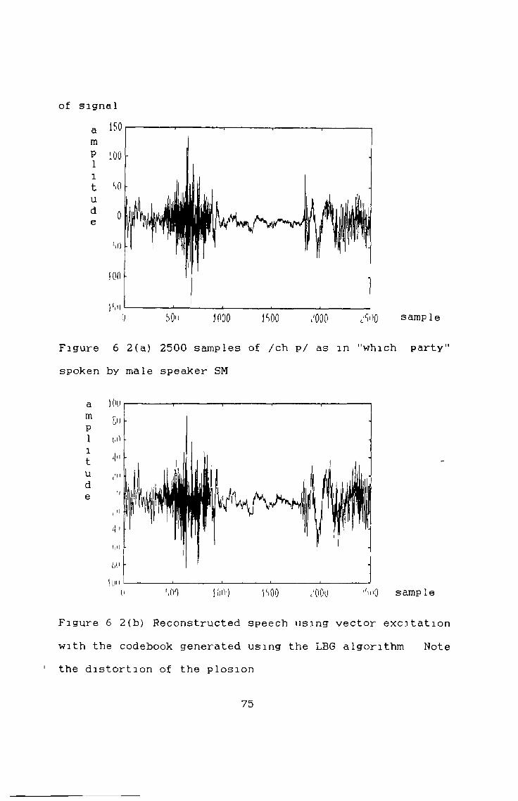
Figure 6 2(a) 2500 samples of /ch p/ as m "which party" spoken by male speaker SM

j00>) N )0 ,'OOU itiQ sample

Figure 6 2(b) Reconstructed speech using vector excitation with the codebook generated using the LBG algorithm Note the distortion of the plosion

75

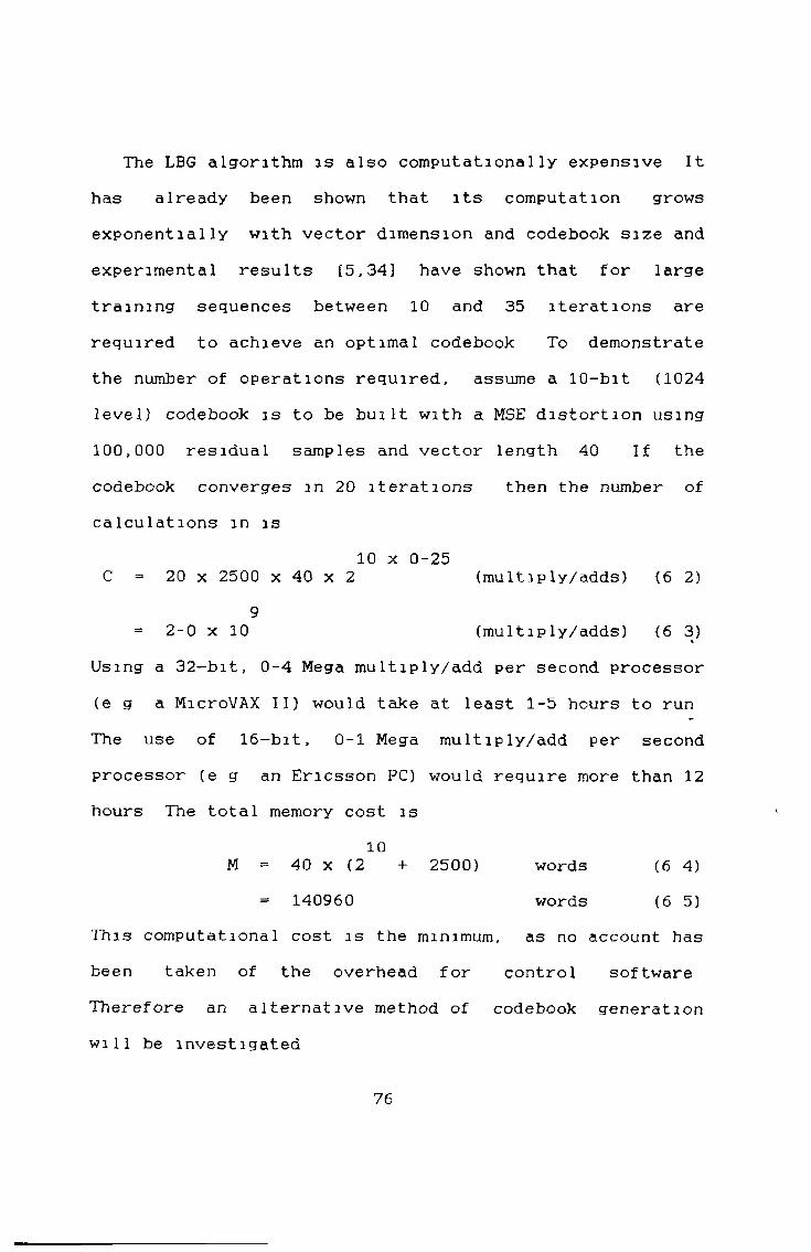
The LBG algorithm is also computationally expensive It has already been shown that its computation grows exponentially with vector dimension and codebook size and experimental results [5,343 have shown that for largetraining sequences between 10 and 35 iterat ions are required to achieve an optima1 codebook To demonstratethe number of operations required, assume a 10-bit (1024level) codebook is to be built with a MSE distortion using 100,000 residual samples and vector length 40 If the codebook converges in 2 0 iterations then the number ofcalculations m is

10 x 0-25C = 20 x 2500 x 40 x 2 (multiply/adds) ( 6 2 )

92 - 0 x 1 0 (multiply/adds) ( 6 3 )

Using a 32-bit, 0-4 Mega multiply/add per second processor (eg a MicroVAX II) would take at least 1-5 hours to run The use of 16-bit, 0-1 Mega multiply/add per secondprocessor (e g an Ericsson PC) would require more than 12hours The total memory cost is

10M = 40 x (2 + 2500) words ( 6 4)

= 140960 words ( 6 5)This computatlona1 cost is the minimum, as no account has been taken of the overhead for control software Therefore an alternative method of codebook generation will be investigated

76

6 4 Pairwise Nearest Neighbour Clustering AlgorithmThe process of generating VQ codewords has already been

described as a process of grouping the training sequence into clusters and then representing each cluster by a single codeword The PNN algorithm starts by assigning a cluster to each vector in the training sequence Then the two vectors that are closest together (according to some distortion measure) are combined together The process then continues until the desired number of clusters is reached

When two vectors are combined into a cluster, they are usually represented by their centroid In N-dimensional Euclidean space this is given by

1cent (C ) - 2 x ( 6 6 )

i M x € C il 1 1

where M is the number of vectors in each cluster C i l

If one assumes that each cluster is adequatelyrepresented by it's centroid, then it is possible tooptimally derive a K-l dimension codebook from a Kdimension codebook This is done by combining the twoclusters which minimise the additional distortionintroduced in representing them as one As with the K~means algorithm, the codebook generated cannot beconsidered globally optimal If the MSE distortion isused 1 on codebook C then the pair of clusters which cause

77

the minimum distortion between clusters C and C is giveni J

byn n i J

--------- I X ~ * |2 (6 7)n + n i ji J

where n is the number of the elements in cluster i and 2 i i

is the centroid of cluster i The only parameters thathave to be updated when calculating equation (6 2) foreach cluster are the weight n and the centroid St Equitz

i l[5] calls the distortion introduced by combining the twoclusters the "weighted distance" because it is a productof the Euclidean distance between the centroids of thecells and the weight of each cell

Once the closest cells have been determined they arecombined taking into account the weight of each centroidso that the "true" centroid is always maintained This iscalculated by

n n n i i J J

2 * - (6 8)n + n i J

where is the centroid of the cluster containing allvectors m C and C

i JIf the algorithm only combines two vectors at each

iteration the computational cost for the training set is

78

Usually the number of training vectors M, is much greater than codebook size L, so this procedure is more expensive than LBG

A more efficient method is to merge more than two vectors at a time If 50% of candidate vectors are combined simultaneously, and then the clusters are readjusted to take account of the combined vectors, equation (6 4) reduces to

NRC « 2MN2 (6 10)

This shortcut, called simple PNN, is only possible if the vectors can be pre-arranged in groups with similar characteristics Methods for accomplishing this will be considered in the next chapter The cost of this algorithm is constant for a given number of training vectors If the numerical example in section (5 2) is applied to equation (6 10) the computation is

8C * 2 x 10

l e about 10% LBG algorithm

6 5 Analysis of the PNN AlgorithmThe PNN algorithm was implemented in the C language on

an Ericsson PC XT The codebook was generated m a similar way to that m section (6 3) and tested using the same

NRC = (M-L) MN2 (6 9)

79

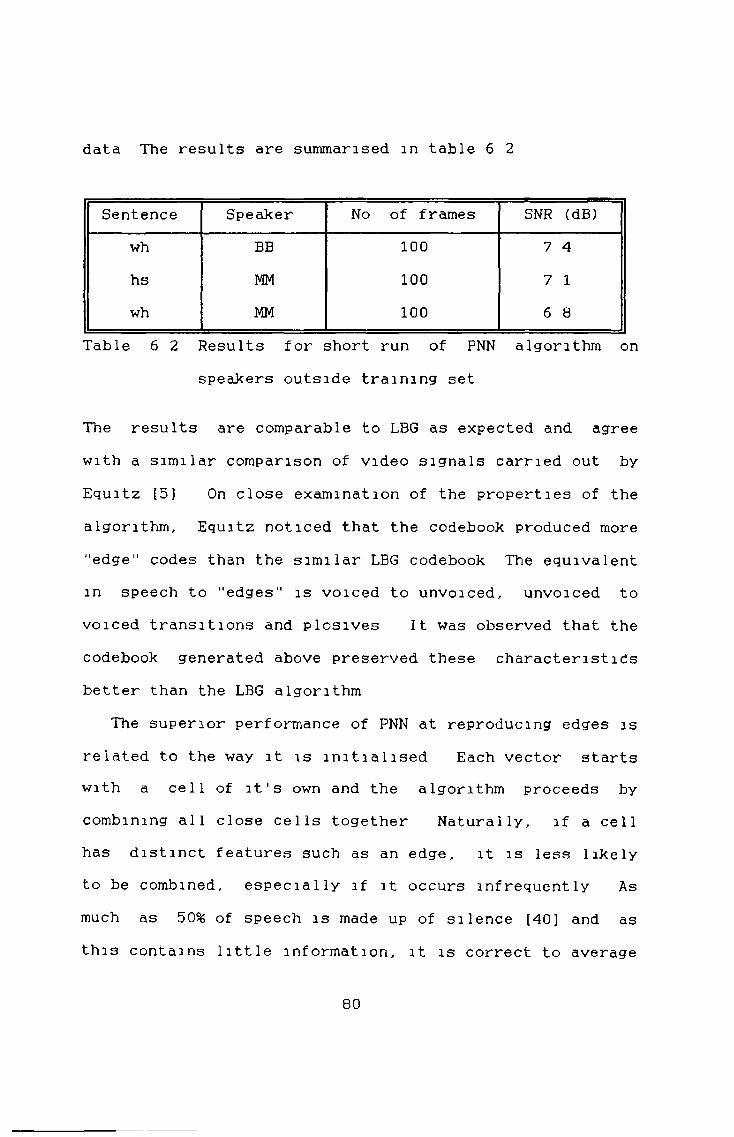
data The results are summarised in table 6 2

Sentence Speaker No of frames SNR (dB)wh BB 100 7 4hs MM 100 7 1wh MM 100 6 8

Table 6 2 Results for short run of PNN algorithm on speakers outside training set

The results are comparable to LBG as expected and agree with a similar comparison of video signals carried out by Equitz [5] On close examination of the properties of the algorithm, Equitz noticed that the codebook produced more "edge” codes than the similar LBG codebook The equivalent in speech to “edges" is voiced to unvoiced, unvoiced to voiced transitions and plosives It was observed that the codebook generated above preserved these characteristics better than the LBG algorithm

The superior performance of PNN at reproducing edges is related to the way it is initialised Each vector starts with a cell of it's own and the algorithm proceeds by combining all close cells together Naturally, if a cell has distinct features such as an edge, it is less likely to be combined, especially if it occurs infrequently As much as 50% of speech is made up of silence [40] and as this contains little information, it is correct to average

80

it into few cells Vowel sounds take up a large proportion of the spoken portion of speech These occupy a large number of cells Unvoiced sounds occupy some cells of their own but also combine with silence cells PNN succeeds, in most cases, to combine the vectors in this way leaving a lot more cells for edges relative to LBG It is also less likely to combine cells with large differences

In the next chapter a method will be described which will reduce the complexity of the codebook search by dividing the full search codebook into logical sub-groups This technique will also enable the simple PNN algorithm to be implemented

81

7 Classification of the LPC Residual

7 1 IntroductionA method for classifying the LPC residual is now

proposed The motivation for classification is to divide the incoming speech into logical subgroups to ease codebook generation and reduce the computational load in searching It was pointed out m the previous chapter that clustering of vectors with similar characteristics would result in substantial computational savings in the PNN a lgon thm

Two systems of classifier were developed The first system is the original CELP idea of comparing the re- synthesised speech for every residual m the codebook, with the speech to be coded This is shown to be prohibitively expensive, but the quality is superior and is used as a benchmark The second system has a more complex three parameter classifier but only residuals are compared

The classification of the residual results in a sub- optimal quantiser because the distortion is no longer minimised over the whole of the codebook However, it will be demonstrated that classification helps to improve the operation of the PNN algorithm by further helping to preserve plosives and other rapidly changing speech

82

signa Is

For classification parameters to be useful they must group the vector together in some subjectively meaningful way The cost of generating the parameters should be taken into account as the reason for using them is to cut down on the computation of a full search codebook Five different measures are described They are (i) Zero Cross Rating (ZCR)

This is a useful parameter for separating high and low frequency signals It was used by Coppen and Sereno [41] along with frame variance to classify an LPC residual without pitch prediction It can be calculated from

N— 12 Isgn[x(m)] - sgn[x(m-l)]| (7 1)

m=0

1 x(n) > 00 x(n) = 0

- -1 x(n) < 0 (7 2)The cost of this measure is approximately 64,000 multiply/adds per second for a vector of 40 samples(1 1 ) Normalised Unit Lag Autocorrelation (PRD)

The parameter is a measure of the periodicity of the residual Although most residuals look totally random, it has been found by experimentation that the unit lag

7 2 Choice of Classification Parameters

83

ZCR

wheresgn[x(n)]

autocorrelation still gives a meaningful measure of periodicity It was used by Cuperman and Gersho [42] who used it in a three way classifier The cost of this measure is approximately 16,000 multiply/adds per second for a 40 sample vectors( m ) Normalised Value of Autocorrelation at Pitch Lag (RPP)

This is proposed as another measure of periodicity It is calculated from the LPC residual as part of the pitch predictor algorithm Therefore there is no direct overhead in generating it However, since it does not give a measure of the actual waveform to be quantised its use must be questioned(iv) Pulsive Measure I (PMI) Ratio of Geometric Mean to Rectified Arithmetic Mean

This pulsive measure proposed by Thomson and Prezas[43] is given by

1 N 2 e2N n=l n

1 N 2 | e |N n=l n

(7 3)It was used as a voiced/unvoiced classifier to improve the excitation of the LPC system In the system to bedescribed it will be used to differentiate between noise

84

like residuals and pulsive ones Therefore it should lump plosives and periodic signals together Another parameter in the classifier will then have to be used to separate out these two signal types (eg a periodicity measure) The computational cost for this measure, assuming a 40 sample vector is 17,000 multiply/adds per second(v) Pulsive Measure II (PMII) Normalised EnergyDifference Function

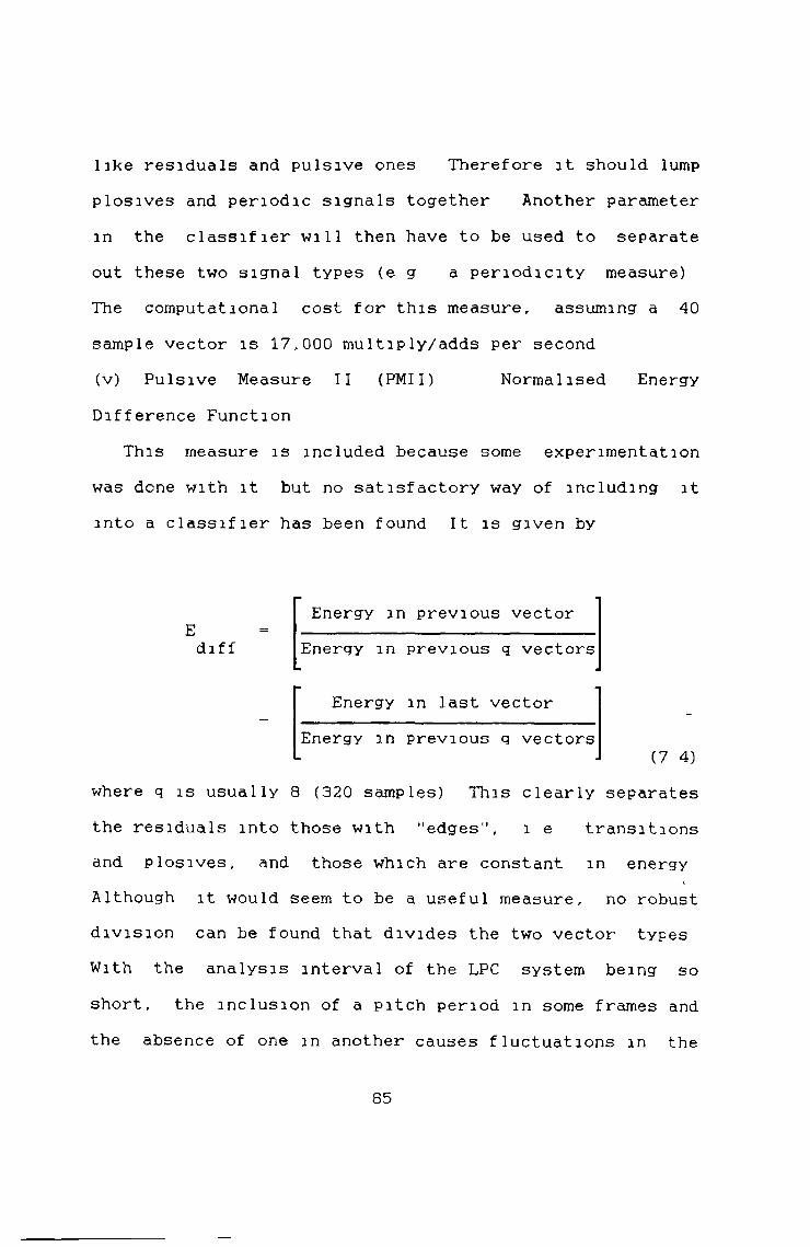
This measure is included because some experimentation was done with it but no satisfactory way of including it into a classifier has been found It is given by

diffEnergy in previous vector

Energy m previous q vectors

Energy m last vector Energy m previous q vectors

(7 4)where q is usually 8 (320 samples) This clearly separates the residuals into those with "edges", l e transitionsand plosives, and those which are constant in energy

\

Although it would seem to be a useful measure, no robust division can be found that divides the two vector types With the analysis interval of the LPC system being so short, the inclusion of a pitch period in some frames and the absence of one in another causes fluctuations m the

85

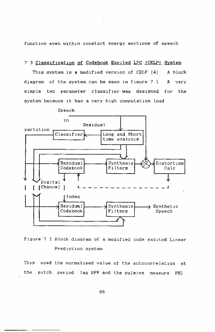
function even within constant energy sections of speech

7 3 Classification of Codebook Excited LPC (CELP) System This system is a modified version of CELP [4] A block

diagram of the system can be seen m figure 7 1 A very simple two parameter classifier was designed for the system because it has a very high computation load

Speech m

Residualpartition

Classif 1 er *r

Digital r rI I I Channel |

I ndexResidualCodebook

Long and Short time analysis

Residual ------- )_____ ^ ___Synthesis Distort ion

Codebook FiIters vO / Calc

i

Synthesis FiIters

Synthetic Speech

Figure 7 1 Block diagram of a modified code excited Linear Prediction system

This used the normalised value of the autocorrelation at the pitch period lag RPP and the pulsive measure PMI

86

These only contribute about 17,000 multiply/adds per second to the computation The codebook was generated using the PNN algorithm This CCELP system was simulated on a MicroVAX II computer The speech database is 32s of a male speaker (SM) reading a passage from a book (Flanagan pg 386 [40]) The test data was four short sentences (seeAppendix I) spoken by a male speaker (BB) and a female speaker (MM), l e all tests were done out of the training sequence with speakers outside the training set

Initially the number of classes was set at four and the codebook size to 64 vectors By experimentation with scatter plots, the parameters were set to RPP=0~5 and PMI=l-5 Table 7 1 shows the effect of varying these parameters on the SNR

PM I RPP SNR(dB)1-5 0-5 8-21-5 0-3 8-51-5 0-2 8-11-8 0-3 9-41-9 0-3 8-6

Table 7 1 Effects of classification thresholds on four class, 64 vector per class CCELP system

In this CCELP system the number of classes has little

87

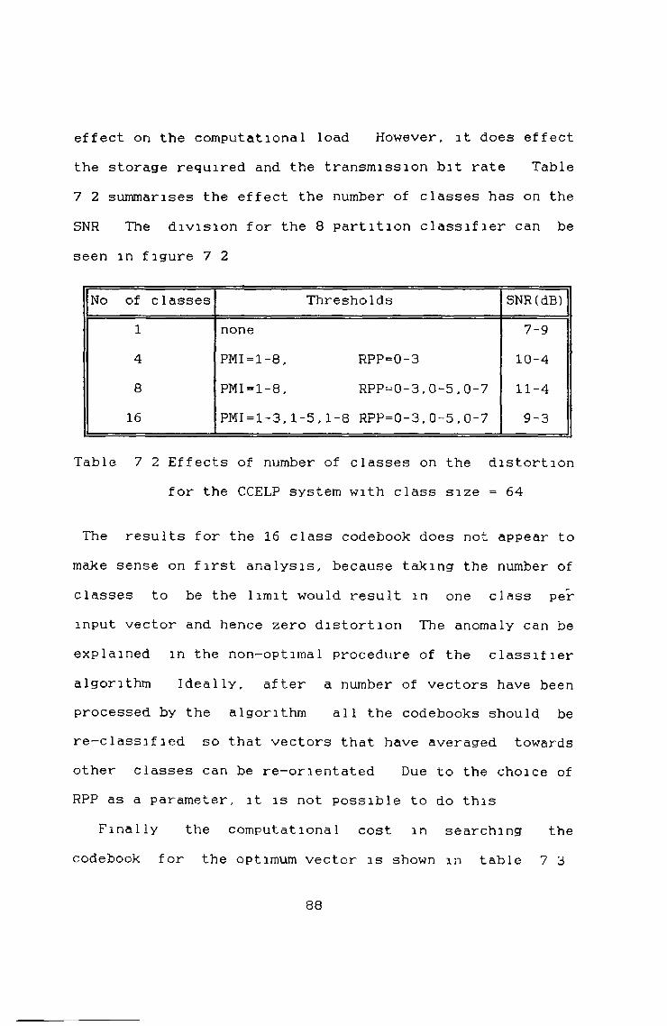
effect on the computational load However, it does effect the storage required and the transmission bit rate Table 7 2 summarises the effect the number of classes has on the SNR The division for the 8 partition classifier can be seen in figure 7 2

No of classes Thresholds SNR(dB)1 none 7-94 PMI=l-8, RPP=0-3 10-48 PMI=l-8, RPP=0-3,0-5,0-7 11-416 PMI=1-3,1-5,1-8 RPP=0-3,0-5,0-7 9-3

Table 7 2 Effects of number of classes on the distortionfor the CCELP system with class size = 64

The results for the 16 class codebook does not appear to make sense on first analysis, because taking the number of classes to be the limit would result m one class perinput vector and hence zero distortion The anomaly can be explained in the non-optimal procedure of the classifier algorithm Ideally, after a number of vectors have been processed by the algorithm all the codebooks should be re-classifled so that vectors that have averaged towards other classes can be re-orlentated Due to the choice of RPP as a parameter, it is not possible to do this

Finally the computational cost m searching thecodebook for the optimum vector is shown m table 7 3

88

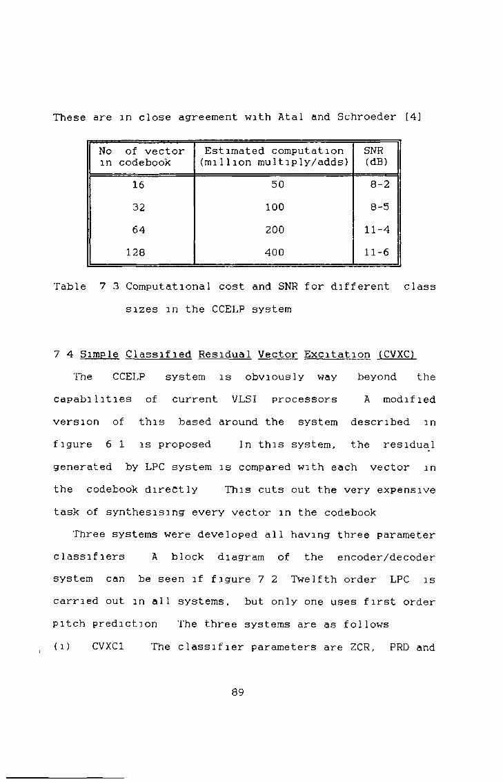
These are m close agreement with Atal and Schroeder [4]

No of vector m codebook

Estimated computation (million multiply/adds)

SNR(dB)

16 50 8-232 100 8-564 200 11-4

128 400 11 **6

Table 7 3 Computational cost and SNR for different class sizes m the CCELP system

7 4 Simple Classifled Residual Vector Excitation (CVXC)The CCELP system is obviously way beyond the

capabilities of current VLSI processors A modified version of this based around the system described in figure 6 1 is proposed In this system, the residual generated by LPC system is compared with each vector in the codebook directly This cuts out the very expensive task of synthesising every vector in the codebook

Three systems were developed all having three parameter classifiers A block diagram of the encoder/decoder system can be seen if figure 7 2 Twelfth order LPC is carried out in all systems, but only one uses first order pitch prediction The three systems are as follows(i) CVXC1 The classifier parameters are ZCR, PRD and

89

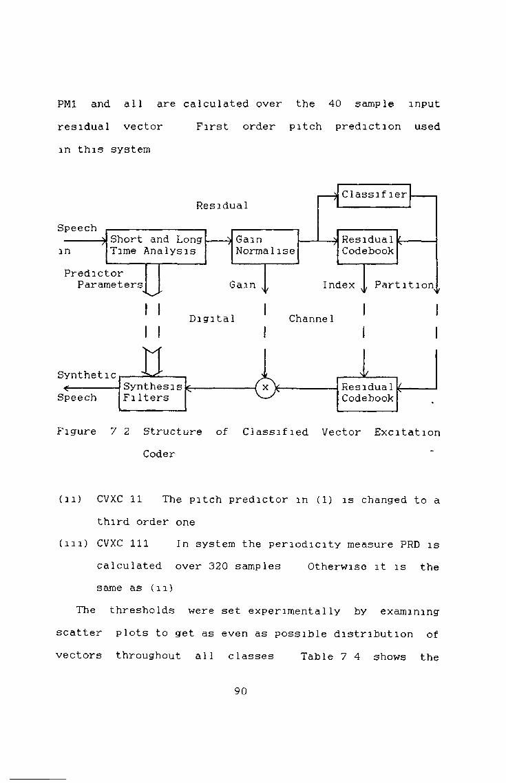
PM1 and all are calculated over the 40 sample input residual vector First order pitch prediction usedin this system

Digital Channel

Figure 7 2 Structure of Classified Vector Excitation Coder

(n) CVXC 11 The pitch predictor m (1) is changed to a third order one

( m ) CVXC 111 In system the periodicity measure PRD is calculated over 320 samples Otherwise it is the same as (n)

The thresholds were set experimentally by examining scatter plots to get as even as possible distribution of vectors throughout all classes Table 7 4 shows the

90

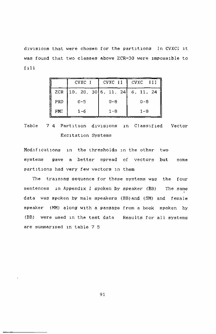
divisions that were chosen for the partitions In CVXCI it was found that two classes above ZCR=30 were impossible to fill

CVXC I CVXC II CVXC IIIZCR PRD PM I

10, 20, 300-51-6

0300

00 1

1 O

«H

6, 11, 24 0 - 8

1-8

Table 7 4 Partition divisions m Classified Vector Excitation Systems

Modifications m the thresholds in the other two systems gave a better spread of vectors but some partitions had very few vectors in them

The training sequence for these systems was the four sentences in Appendix I spoken by speaker (BB) The same data was spoken by male speakers (BB)and (SM) and female speaker (MM) along with a passage from a book spoken by (BB) were used in the test data Results for all systems are summarised in table 7 5

91

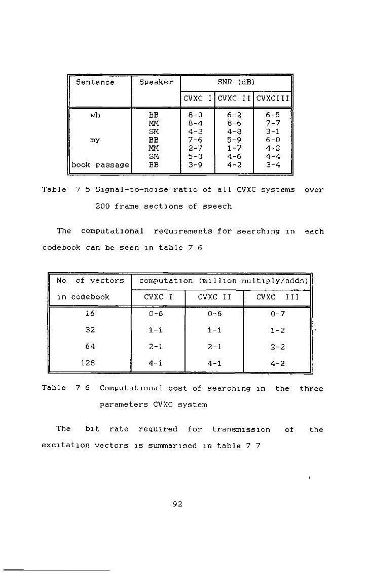
Sentence Speaker SNR (dB)CVXC I CVXC II CVXCIII

wh BB 8-0 6-2 6-5MM 8-4 8-6 7-7SM 4-3 4-8 3-1

my BB 7-6 5-9 6-0MM 2-7 1-7 4-2SM 5-0 4-6 4-4

book passage BB 3-9 4-2 3-4

Table 7 5 Signal-to-noise ratio of all CVXC systems over 200 frame sections of speech

The computational requirements for searching m each codebook can be seen in table 7 6

No of vectors in codebook

computation (million multiply/adds)CVXC I CVXC II CVXC 111

16 io VOio 0 1 SI

32 1-1 1-1 1-264 2-1 2-1 CM1CM

128 <—i i 4-1 4-2

Table 7 6 Computational cost of searching in the three parameters CVXC system

The bit rate required for transmission of the excitation vectors is summarised m table 7 7

92

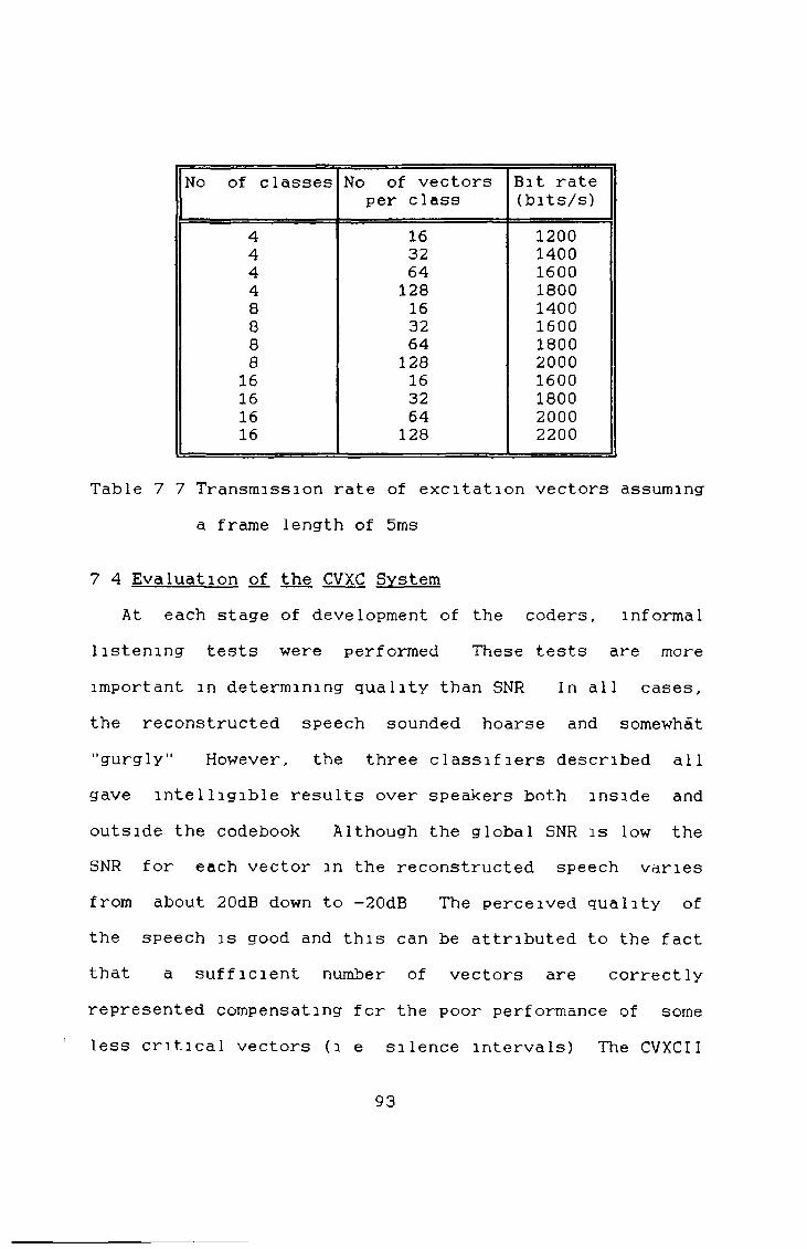
No of classes No of vectors per class

Bit rate (bits/s)

4 16 12004 32 14004 64 16004 128 18008 16 14008 32 16008 64 18008 128 200016 16 160016 32 180016 64 200016 128 2200

Table 7 7 Transmission rate of excitation vectors assuming a frame length of 5ms

7 4 Evaluation of the CVXC SystemAt each stage of development of the coders, informal

listening tests were performed These tests are more important in determining quality than SNR In all cases, the reconstructed speech sounded hoarse and somewhat "gurgly" However, the three classifiers described all gave intelligible results over speakers both inside andoutside the codebook Although the global SNR is low theSNR for each vector in the reconstructed speech varies from about 20dB down to -20dB The perceived quaiity ofthe speech is good and this can be attributed to the factthat a sufficient number of vectors are correctly represented compensating for the poor performance of some less critical vectors (i e silence intervals) The CVXCII

93

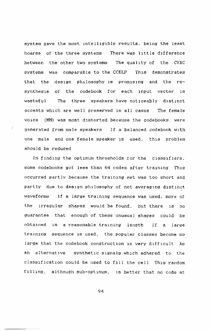
system gave the most intelligible results, being the least hoarse of the three systems There was little difference between the other two systems The quality of the CVXC systems was comparable to the CCELP This demonstrates that the design philosophy is promising and the re- synthesis of the codebook for each input vector is wasteful The three speakers have noticeably distinct accents which are well preserved in all cases The female voice (MM) was most distorted because the codebooks were generated from male speakers If a balanced codebook with one male and one female speaker is used, this problem should be reduced

In finding the optimum thresholds for the classifiers, some codebooks got less than 64 codes after training This occurred partly because the training set was too short and partly due to design philosophy of not averaging distinct waveforms If a large training sequence was used, more of the irregular shapes would be found, but there is no guarantee that enough of these unusual shapes could be obtained in a reasonable training length If a large training sequence is used, the popular classes become so large that the codebook construction is very difficult As an alternative synthetic signals which adhered to the classification could be used to fill the cell This random filling, although sub-optimum, is better that no code at

94

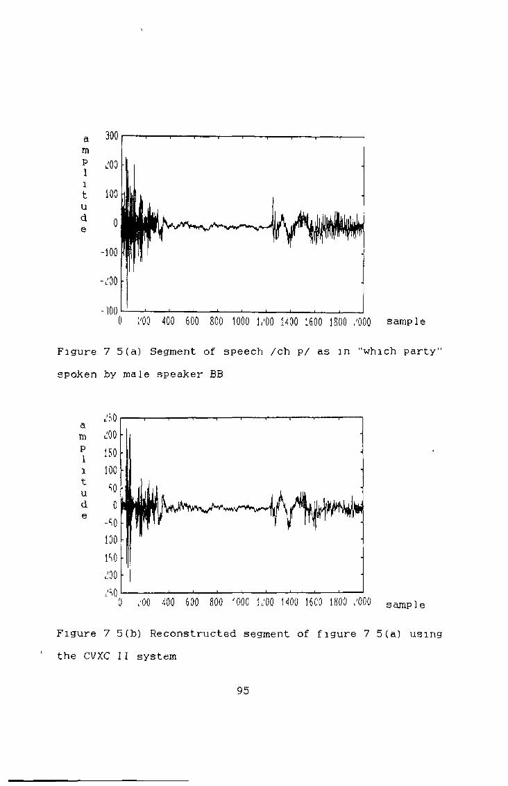
800 1000 1/00 1400 1600 1800 /000 sample

Figure 7 5(a) Segment of speech /ch p/ as in ’’which party" spoken by male speaker BB

Figure 7 5(b) Reconstructed segment of figure 7 5(a) using the CVXC 11 system

95

It was stated that one area of improvement most hoped for over traditional excitation methods was the reconstruction of plosives Figure 7 5 (a) shows thesegment /ch p/ of the words "which party" spoken by (BB) inside the codebook for the CVXCII system The processed and reconstructed versions of this can be seen in figure 7 5(b) The characteristic shape of the plosive is well preserved, as is the shape of most of the surrounding speech The gain at this frame was low so the actual size of the plosion was reduced This good reproduction of plosives was borne out m listening tests

all

96

8 Improvements and Future Developments

8 1 IntroductionFurther work remains to be done to complete the

investigation of the classifier in the CVXC system This chapter outlines a set of comprehensive tests that must be carried out so that the classifier can reach its full potential Noise shaping is then described This can be used to reduce noise at frequencies where speech power is low, and so improve perceived quality The possibility of incorporating another coding technique (multi-pulse) is discussed An alternative matching procedure is proposed which get around the limitations of the squared error distortion measure

Finally, the hardware required for the implementation of the whole CVXC system is described It is demonstrated that the use of the very latest DSP chips enables this to be carried out in real time

8 2 Improving the CodebookSo far, all the results obtained have been for

codebooks generated from short length training sequence (<32s) The results have been promising but not comprehensive The first recommendation and the one that should probably have the greatest effect, is to use a

97

training sequence of 5 minutes This should contain at least five male and five female speakers so that the widest range of speech characteristics are covered The partition parameters could then be further refined

Computationally, the extension of the training set is very high Five minutes of residuals takes up almost 5M bytes of memory In the CVXC systems described previously, 50% of the input vector went into five different partitions On average, this means that in one of these partitions 6000 vectors will have to be compressed into 64 vectors Using simple PNN, this means at least 30M multiply/adds per partition Therefore, to efficiently carry out further investigations, more powerful hardware will be required

When using the simplified PNN algorithm, it is necessary to re-classify the codebook after each step A periodicity measure must be found that is tractable over the vector length and gives better results than PRD m the "VXC II system This would stop the problem of a codebook oeing generated in a partition which would never be used

J 3 Perceptual Noise WeightingThe hoarseness that the coded speech suffers from is

lainly due to high noise levels at low frequencies Galand 7] showed that the pre-emphasis filter of the form

98

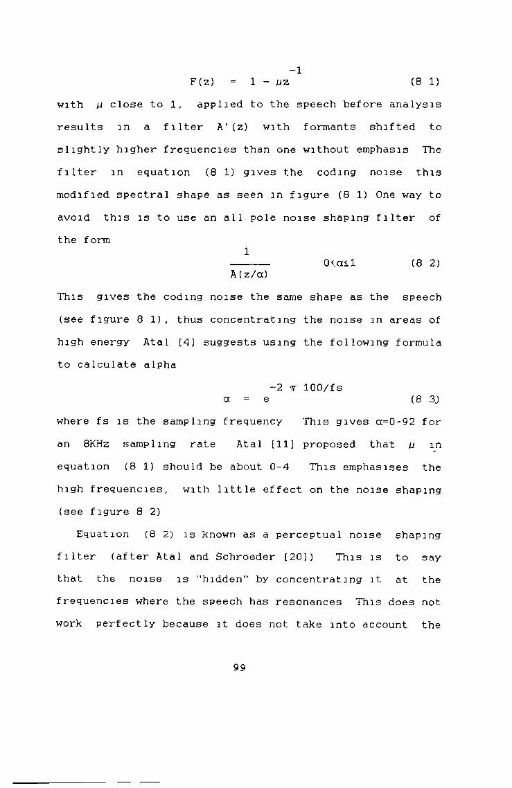
with u close to 1, applied to the speech before analysis results in a filter A ’(z) with formants shifted to slightly higher frequencies than one without emphasis The filter in equation (8 1) gives the coding noise this modified spectral shape as seen in figure (8 1) One way to avoid this is to use an all pole noise shaping filter of the form

1------------ Oiccil (8 2)A(z/a)

This gives the coding noise the same shape as the speech (see figure 8 1), thus concentrating the noise in areas of high energy Atal [4] suggests using the following formula to calculate alpha

-2 7T 100/fs a = e (8 3J

where fs is the sampling frequency This gives a=0-92 foran 8KHz sampling rate Atal [11] proposed that u inequation (8 1) should be about 0-4 This emphasises thehigh frequencies, with little effect on the noise shaping(see figure 8 2)

Equation (8 2) is Known as a perceptual noise shapingfilter (after Atal and Schroeder [20]) This is to saythat the noise is "hidden" by concentrating it at thefrequencies where the speech has resonances This does notwork perfectly because it does not taKe into account the

-1F(z) 1 - uz (8 1)

99

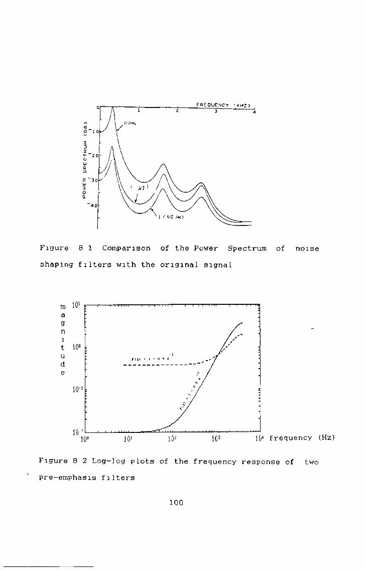
Figure 8 1 Comparison of the Power Spectrum of noise

3haping filters with the original signal

Figure 8 2 Log— log plots of the frequency response of two pre-emphasis filters

100

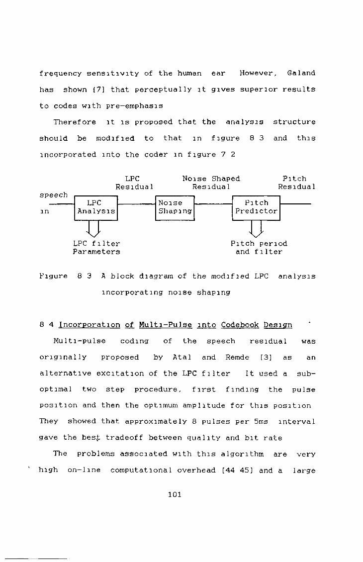
frequency sensitivity of the human ear However, Galand has shown [73 that perceptually it gives superior results to codes with pre-emphasis

Therefore it is proposed that the analysis structure should be modified to that in figure 8 3 and this incorporated into the coder m figure 7 2

LPCResidual

Noise Shaped Residua 1

PitchResidual

LPC filter Parameters

Pitch period and filter

Figure 8 3 A block diagram of the modified LPC analysis incorporating noise shaping

8 4 Incorporation of Multi-Pulse into Codebook DesignMulti-pulse coding of the speech residual was

originally proposed by Atal and Remde [3] as an alternative excitation of the LPC filter It used a sub- optimal two step procedure, first finding the pulse position and then the optimum amplitude for this position They showed that approximately 8 pulses per Sms interval gave the bes£ tradeoff between quality and bit rate

The problems associated with this algorithm are very high on-line computational overhead [44 453 and a large

101

distortion when the bit rate is reduced below 8k bit/s[44)

The incorporation of multi-pulse techniques into VXC was proposed by Davidson and Gersho [46 3 They showed that the vectors could be stripped down to 4 pulses per 40 dimension vector This produced a small increase in the perceived quality of the speech The thinning out procedure results in a 10% reduction m the storagerequirements It also reduces the search complexity of the coder Unfortunately, it adds significantly to the codebook generation complexity

An experimental investigation of this method to see how well it works on codes generated by the PNN algorithm is needed before steps could be taken to incorporate multi- pulse into the present system

8 5 A1ternative Search ProcedureIt was demonstrated that CELP could achieve better

SNR than the CVXC systems This demonstrates the weaknessof the squared error distortion measure on its ownAlthough it may match waveforms reasonably well, noconsideration is taken of the speech that is generated No distortion measure short of the complexity of CELP can directly determine the perceptual quality of each code vector

102

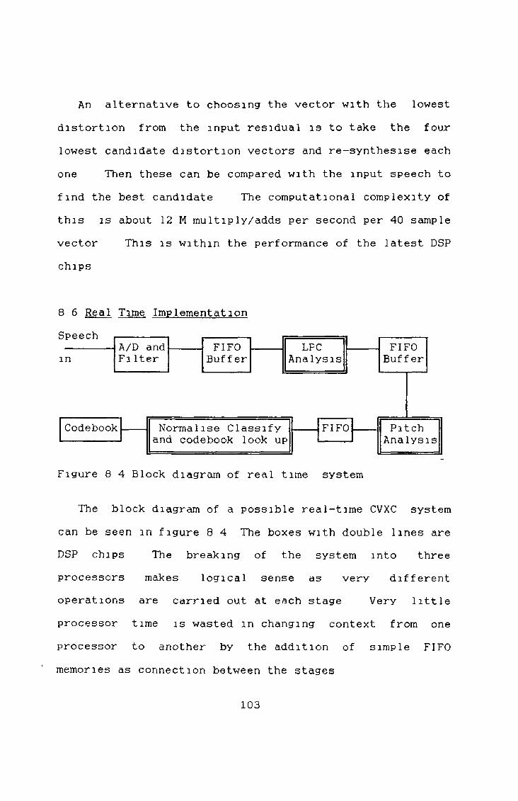
An alternative to choosing the vector with the lowest distortion from the input residual is to take the four lowest candidate distortion vectors and re-synthesise each one Then these can be compared with the input speech to find the best candidate The computational complexity of this is about 12 M multiply/adds per second per 40 sample vector This is within the performance of the latest DSP chips

8 6 Real Time Implementation

Figure 8 4 Block diagram of real time system

The block diagram of a possible real-time CVXC system can be seen in figure 8 4 The boxes with double lines are DSP chips The breaking of the system into threeprocessors makes logical sense as very differentoperations are carried out at each stage Very little processor time is wasted in changing context from one processor to another by the addition of simple FIFO memories as connection between the stages

103

The implementations of LPC analysis described in chapter 4 required about 6 M instructions per second A fixed point implementation on a 32 bit DSP would reduce this to about 4 M instructions per second The pitch analysis is very expensive, mainly due to the calculation of the autocorrelation Shortcuts in this calculation can be achieved by using the FFT method [123 which cut down the calculations to 15 M instructions per second Other shortcuts, such as reducing the computation of the comb filter by complex buffering of the filter delays would reduce the computation by as much as another 5M instruction per second

Chapter 7 described a range of possible classifications systems that could be implemented If a 2,000 bits/sec transmission rate for the residual is required only a 2 million multiply/adds per sec processor is required However, if the modification suggested in section 8 5 is added a further 12 million multiply/adds per sec would be required

The addition of Vector Quantisation to the predictor parameters would require the addition of another processor The speed of this would be dependent on the size of code book needed Using a 1024 level binary tree codebook for LPC parameters would be about the same as the Durbin recursion [363 The pitch and gain quantisation

104

is much simpler so a-processor of less than 5 multiply/adds per second would suffice for this

mi 11 ion

105

9 Conelusions

An investigation of the elements of a Classified Vector Excitation System was carried out LinearPredictive coding was studied m detail and it was found that it gave a good representation of the spectral shape of most speech sounds However the residual still contained some information which it was necessary to transmit to a decoder for accurate speech reconstruction

Previous techniques for accomplishing this were investigated The traditional voiced/unvoicedsynthesiser is totally inadequate for high quality reproduction Waveforms Vector Quantisation was then studied as a way of improving excitation The LBG algorithm was seen to give reasonable results in some speech areas, but was unable to reproduce plosives accurately

An alternative to this algorithm, called Pairwise Nearest Neighbour clustering, was applied to speech This gave improved results m the reconstruction of plosives and reasonable results in most other areas

Classification of the residual was then described This technique divided up the code book into segments with common characteristics This resulted in much reduced search complexity and also enabled a shortcut in the PNN

106

algorithm to be carried out It further enhanced the preservation of "edge" codes m the speech

The results obtained were based on very short training sequences Although the SNR was low, especially m the case of the CVXC system, the speech was always intelligible The reproduced speech was "gurgly" and a little hoarse It is imperative that a longer training sequence be tried before a definitive statement on the usefulness of this system can be made However, the robustness of the system from speaker to speaker is encouraging Adding the recommendations in chapter 8 should result in noticeable improvements

To sum up, the PNN algorithm is a useful alternative to the LBG or K-means algorithm for code book design Classification of the residual helps the code book search effort, it streamlines PNN codebook generation and reduces the distortion of "edge" type residuals

107

10 Biblography

[1] B S Atal and M R Schroeder, "Adaptive Predictive Coding of Speech Signals*', Bel 1 Syst Tech J , Vol 49 , PP 1973-1987, Oct 1970[2] F I Itakura and S Saito, "Analysis-SynthesisTelephony Based Upon the Maximum Likelihood Method", Proc th

6 Int Congress on Acoustics, pp C17-20, Tokyo 1968[3] B S Atal and J R Remde, "A New Model of LPC Excitation for Producing Natural-sounding speech at low bit rates", Proc of ICASSP, pp 614-617, Paris 1982[4] M R Schroeder and B S Atal, "Stocastic Coding of Speech Signals at Very Low Bit RatThe Importance of Speech Perception", Speech Communication, Vol 4, pp 155- 162, North-Holland 1985[5] W Equitz, "Fast Algorithms for Vector Quantisation Picture Coding”, Proc of ICASSP, pp 725-728, Dallas, Tx 1987[6] S Marlow and B Buggy, "Selective Modelling of the LPC Residual", To be published in Proc of European Speech Technology Conference, Edinburgh 1987[7] C Galand, "Theoretical and Experimental Study of Adaptive Predictive Coders", Proc ICASSP, pp 619-622, Atlanta, G1981

108

i

[8] J L Flanagan, M R Schroeder B S Atal, R E Crochiere, N S Jayant and J M Tnbolet, "Speech Coding", IEEE Trans on Commun Vol COM-27, No 4, p p

710-737 April 1979[9] J Makhoul, "Linear Prediction A Tutorial Review", Proc IEEE Vol 63, p p 561-580, April 1975[10] J Makhoul, "Stable and Efficient Methods for Linear Prediction", IEEE Trans Acoust . Speech, Signal Processing. Vol ASSP-25, No 5, p p 423-428, Oct 1977[11] B S Atal, "Predictive Coding of Speech at Low BitRates" IEEE Trans on Commun Vol CÖM-30 No 4, p p

600-614, April 1982[12] L R Rabiner and R W Schafer, Digital Processing of Speech Signals, Englewood Cliffs NJ Prentice-Hal1,1971[13] S Chandra and W C Lin "Experimental Comparisonbetween Stationery and Non-stationery Formulations of Linear Prediction Applied to Speech" IEEE Trans Acoust Speech, Signal Processing, Vol ASSP-22 No 5 p p 403-415, Oct 1977[14] B S Atal and S L Hanauer, "Speech Analysis andSynthesis by Linear Prediction of the Speech Wave" JAcoust Soc Am Vol 50, p p 637-655, 1971[15] J D Marke 1 and A H Gray Jr Linear Prediction ofSpeech New York NY Springer Verlag, 1976

109

[16] A V Oppenheim and R W Schafer, Digital Signal Processing, Englewood Cliffs, NJ Prentice-Hal1, 1975[17] J Burg, "A New Analysis Technique for Time SeriesData“, Proc NATO Advanced Study Institute on SignalProc , Enschede, Netherlands, 1968[18] N Levinson, ’’The Wiener RMS (root mean square) Error Criterion in Filter Design and Prediction", J_ Math Phys , Vo 1 25, p p 261-278, 1947[19] J Durbin, ’'The Fitting of Time Series Models", Rev Intern Statist Inst , Vol 28, p p 233-244, 1960[20] B S Atal and M R Schroeder, "Predictive Coding of Speech Signals and Subjective Error Criteria", IEEE Trans Acoust , Speech, Signal Processing, Vol ASSP-27, No 3,June 1977[21] B S Atal, "High Quality Speech at Low Bit Rates Multi-Pulse and Stochastically Excited Linear Predictive Coders", Proc ICASSP p p 1681-1684, Tokyo 1986[22] S T Alexander and Z M Rhee, "Analytical FinitePrecision Results for Burg's Algorithm and theAutocorrelation Method for Linear Prediction", IEEE Trans Acoust , Speech, Signal Processing, Vol ASSP-35, No 5,May 1987[23] T P Barnwell III, "Windowless Techniques For LPC Analysis" IEEE Trans Acoust , Speech, Signal Processing. Vol ASSP-28, No 4, August 1980

110

[24] A H Gray Jr and D Y Wong, "The Burg Algorithm for LPC Speech Analysis/Synthesis", IEEE Trans Acoust ,Speech, Signal Processing, Voi ASSP-28, No 6, Dec 1980[25] Texas Instruments, TMS32Q20 User1s Guide, Texas Instruments, 1985[26] J Le Roux and C Gueguen, "A Fixed Point Computation of Partial Correlation Coefficients”, IEEE Trans Acoust , Speech, Signal Processing, Voi ASSP-25, No 3, June 1977[27] S Maitra and C R Davis, "A Speech Digitizer at 2400Bits/s", IEEE Trans Acoust , Speech, Signal Processing, Voi ASSP-27, No 6, Dec 1979[28] R M Gray, "Vector Quantization", IEEE ASSP Magazine, April 1984[29] C E Shannon, "A Mathematical Theory of Communication", Bel 1 Syst Tech J , Voi 27, p p 379-423, 623-656, 1948[30] C E Shannon, "Coding Theorems for a Discrete Source with a Fidelity Criterion", IRE Nat Conv Ree (pt 4) , PP 142-163, 1959[31] R Gallager, Information and Reiiable Communication, New York, NY Wiley 1968[32] T Berger, Rate Distortion Theory, Englewood Cliffs, NJ Prentice-Hal1 1971[33] J Makhoul, "Vector Quantization in Speech Coding" Proc IEEE. Voi 73, No 11, Nov 1985

111

[34] Y Linde, A Buzo and R M Gray, "An Algorithm for Vector Quantizer Design”, IEEE Trans Commun , vol COM- 28, No 1, p p 84-95, Jan 1980[35] H Abut, R M Gray and G Rebolledo, ’’Vector Quantization of Speech and Speech-1 ike Waveforms", IEEE Trans Acoust . Speech. Signal Processing, Vol ASSP-30, PP 423-435[36] A Buzo, A H Gray Jr , R M Gray and J D Markel, "Speech Coding Based Upon Vector Quantization", IEEE Trans Acoust , Speech, Signal Processing, Vol ASSP-28, PP 562-574, Oct 1980[37] F Itakura, "Minimum Prediction Residual Principle Applied to Speech Recognition", IEEE Trans Acoust . Speech, Signal Processing, Vol ASSP-23, No 1, pp 67-72, Feb 1975[38] R M Gray, A Buzo, A H Gray Jr , "An 800 Bits/s Vector Quantization LPC Vocoder”, IEEE Trans Acoust , Speech, Signal Processing, Vol ASSP-30, No 5, Oct 1982“[40] J L Flanagan, Speech Analysis Synthesis and Perception, New York, NY Springer Verlag, 1972[41] M Coppen and D Sereno, "Feature Extraction and Product Codes in Vector Excited Coders”, Proc ICASSP, pp 1942-1945, Dallas, TX 1987

112

[42] V Cuperman and A Gersho, "Vector Predictive Coding of Speech at 16k Bits/s", IEEE Trans on Commun , Vol COM-33, July 1985[43] D L Thomson and D P Prezas, "Selective Modeling of the LPC Residual During Unvoiced Frames White Noise or Pulse Excitation", Proc ICASSP, pp 3087-3090, Tokyo 1986[44] S Singhal, "Reducing Computation m Optimal Amplitude Mulit-Pulse Excitation", Proc ICASSP, pp 2363- 2366, Tokyo 1986[45] J Lefevre and M Coppen, "Speech Coding What isthe Need for the Office Workstation", Proc ESPRIT Tech Week, 1985[46] G Davidson and A Gersho, "Complexity Reduction Methods for Vector Excitation Coding", Proc ICASSP, pp 3055-3058, Tokyo 1986

113

Sentence Test SentenceCodewh Which party did Baker go to ?my Many may know my new meaninghs His vicious father had seizuresry Why were you away a year Roy 7

Appendix 1

114