Natural Resources Defense Council Appliance Standards

Natural Resources Defense Council Appliance Standards Awareness Project

October 12, 2012

Ms. Brenda Edwards U.S. Department of Energy Building Technologies Program 1000 Independence Avenue, SW Mailstop EE-2J Washington, DC 20585

RE: Docket No. EERE-2012-BT-STD-0020 / RIN 1904-AC77: Energy Conservation Standards for Commercial Clothes Washers

Dear Ms. Edwards, This letter constitutes the comments of the Natural Resources Defense Council and the Appliance Standards Awareness Project in response to the Department of Energy (DOE) notice of availability of the Framework Document (FD) regarding Energy Conservation Standards for Commercial Clothes Washers (CCWs). 77 Fed. Reg. 48108. We appreciate the opportunity to provide input to this process. All major product categories should be included in the DOE Analysis It should be noted that “other commercial applications” in the statutory definition of this product category include washers used for on-premise laundry. The FD assumes, without citing data, that applications other than coin laundries and multi-housing common areas constitute a “small segment” of the market,1 and the category was largely ignored in the technical analysis for the 2010 rule.2 One of the major venues for on-premise laundry is the hospitality industry. We note that the lodging industry reported nearly 4.9 million guestrooms in 2011 with an occupancy factor of 60% in properties with 15 or more rooms.3 Additionally, the 17,000 bed and breakfast establishments averaged 6 rooms with a reported occupancy of about 44%.4 While large establishments often use larger laundry equipment not covered by the DOE CCW standards, the size of the hospitality industry alone makes on-premise laundry equipment a sector clearly worthy of evaluation in the DOE analysis. And while the total unit count may indeed be smaller than the other two sectors evaluated in the previous analysis, this subgroup may have distinctive usage factors that will influence total energy and water use for covered CCWs.

1 Framework Document, p. 25. 2 See, for example: Commercial Clothes Washers Final Rule Technical Support Document, December 2009. Chapter 6, Energy and Water Use Determination, p. 6-5. “ . . . DOE focused only on these two building applications to determine the appropriate number of commercial clothes washer cycles per year.” 3 American Hotel and Lodging Association, <www.ahla.com>. 4 Professional Association of Innkeepers International. www.inkeeping.org.

1

http://www.inkeeping.org/

Test Procedure Issues The energy savings in CCWs achieved by reducing the remaining moisture content (RMC) of clothing at the end of the wash cycle are largely dependent on moisture-sensing termination controls in commercial dryers. The prevalence of timer-activated termination controls in commercial dryers must be considered. In its 2010 analysis, DOE used its residential clothes washer analysis from the year 2000 to determine a relationship between RMC and MEF for the purpose of calculating the dryer energy for commercial clothes washers.5 Additionally, the effectiveness of automatic termination controls, to the extent they are present in commercial dryers, will also affect energy savings from CCWs that achieve a lower RMC. A 2009 report by Ecos Consulting looking at residential clothes dryers found that termination control strategies can vary in effectiveness and that actual drying energy varied by 20 to 30 percent for the same load, largely because energy use at the end of cycle is not being captured in the current test procedure.6 We support establishing new efficiency standards based on IMEF metric to capture standby and off-mode power and IWF metric to capture water consumption from all temperature cycles. Additionally, the cold temperature usage factor (.37) in the current test procedure should be corroborated for the commercial environment. Reuse of Previous Analyses DOE should specify the portions of the 2010 analysis that will be reused in the current rulemaking, and to what extent data, if not methodology, will be updated. Market Assessment DOE should confirm the split between the coin laundry and multifamily housing sectors of the market. The different operating characteristics of these subsectors have significant influence on the life-cycle costs and payback period analysis, and erroneous estimates of subsector shipments may significantly skew the outcome of the rulemaking. Product Classes DOE must reconsider the division of CCWs into separate product classes for top-loading and front-loading machines. As stated in the FD:

During the previous energy conservation standards rulemaking for CCWs, DOE promulgated standards for two product classes: top-loading and front-loading. DOE stated that it had identified at least one consumer utility related to the method of loading clothes. Specifically, DOE determined that the longer cycle

5 Commercial Clothes Washers Final Rule Technical Support Document, December 2009. Chapter 6, Energy and Water Use Determination, p. 6-3. 6 Bendt, Calwell, and Moorefield. Residential Clothes Dryers: An Investigation of Energy Efficiency Test Procedures and Savings Opportunities. Ecos Consulting. November 6, 2009, pp.4-5.

2

times of front-loading CCWs versus cycle times for top-loaders are likely to significantly impact consumer utility. In commercial and multi-housing settings, it is beneficial to consumers with multiple, sequential laundry loads to approximately match CCW cycle times to those of the dryers to maximize throughput and minimize wait times, and wash times of 70–115 minutes would be longer than most drying cycles. Because the longer wash cycle times for front-loaders arise from the reduced mechanical action of agitation as compared to top-loaders, DOE stated such longer cycles may be required to achieve the necessary cleaning, and thereby constitute a performance-related utility of frontloading CCWs versus top-loading CCWs under the meaning of 42 U.S.C. 6295(q). 75 FR 1122, 1130-34. For the reasons stated above and in the previous rulemaking, DOE is considering retaining these two product classes during this rulemaking.7

In the 2010 final rule, DOE was drawing comparisons from a February 2009 Consumer Reports article on residential washers contrasting front-loader cycle times of 50 to 115 minutes with top-loader cycle times of 30 to 85 minutes. Currently, however, Speed Queen has two models of commercial front loaders with a cycle time of 27 minutes, while two of their models of top-loaders are advertised at 16 to 31 minutes and a third commercial top loader simply advertised as “programmable”. Unimac, which is another Alliance brand, offers comparably sized top and front loaders with respectively the same cycle times with the added note “plus fill time”, which would presumably add at least another minute or two, and may apply to the Speed Queen machines. For comparison, GE’s commercial top loader is listed with a wash time of 24.5 minutes excluding water fill time. And Electrolux has a comparably sized commercial front-loader with a “total time” of 31 minutes. Thus, today’s commercial front loaders operate within the same time range as the top loaders, a fact that obviates DOE’s principal rationale for two separate product classes.8 Technology Assessment Temperature-differentiated pricing controls should be added to the list of technology options that manufacturers can use to reduce energy consumption in machine operation. This feature is already being offered by Whirlpool and by Alliance in their Speed Queen branded products. Temperature differentiated pricing offers launderers the incentive to opt for lower temperature settings than they might otherwise select under undifferentiated pricing. Such controls allow a machine’s owner or leasee to pass through a share of the energy savings resulting from less frequent use of hot water to the end user making the temperature selection. The test procedure for CCWs can allow credit for inclusion of such a feature without altering the mechanics of the test procedure itself.

7 Framework Document, pp. 18-19. 8 DOE previously concluded that first cost is not a “feature” that provides consumer utility for purposes of EPCA, nor is accessing a top-loading washer without stooping a consumer utility when clothes dryers invariably operate in a front-loading format. See 75 Fed. Reg. 1133-1134.

3

Engineering Analysis In the FD, DOE stated that the Department is unaware of any top-loaders that exceed the January 8, 2013 baseline efficiency level and therefore did not identify any efficiency levels above the baseline to analyze.9 However, the absence of current products on the market that exceed the baseline level does not necessarily mean that efficiency levels above the baseline are not technologically feasible. As noted by DOE in the FD, the maximum available efficiency level is not necessarily equivalent to the “max-tech” level since there may be technology options for improving efficiency that have not yet been incorporated into current products.10 If DOE retains separate product classes for top-loaders and front-loaders, DOE must identify a max-tech level for top-loaders. Energy and Water Use Analysis Cycles per year should be determined for on-premise laundries as well as for coin laundries and multifamily housing. Life-Cycle Cost and Payback Period Analysis Energy, Water and Wastewater Prices. The most recent AWWA/Raftelis survey should be used. The 2010 survey contains water price information for 308 utilities and wastewater price information for 228 utilities. Shipments Analysis Energy Star unit shipment data for 2011 implies a total market of approximately 200,000 new CCWs that year.11 Since the program partners supplying data to Energy Star are the manufacturers supplying data to DOE for this analysis, these data points should be reflected in DOE’s shipments analysis. Monetizing Carbon Dioxide and Other Emissions Reductions DOE’s proposed methodology for monetizing carbon dioxide significantly underestimates the benefits associated with CO2 emissions reductions. As argued by NRDC economist Laurie Johnson in a recently published paper in the Journal of Environmental Studies and Sciences, attached as appendix A, the values developed by the interagency committee for social cost of carbon which DOE proposes to use in its analysis significantly underestimate the negative effects that CO2 emissions will have on future generations. As described in detail in Appendix A, the primary flaw in the interagency committee’s analysis is that it does not use appropriate discount rates or discounting methodology for intergenerational costs and benefits (for intergenerational benefits, OMB permits discount rates between 1 and 3 percent, whereas the lowest discount rate used by the committee was 2.5 percent). The study found that CO2 emissions are likely to impose damages between 2.6 to more than 12 times higher than the government’s primary estimate,

9 Framework Document. p. 22. 10 Ibid. p. 23. 11 Energy Star Unit Shipment and Market Penetration Report Calendar Year 2011 Summary. www.energystar.gov.

4

http://www.energystar.gov/

resulting in a range of $55 to $266 per ton. Even these estimates may be too low if future temperature increases are outside the middle range predicted by climate scientists (the $55 to $266 figures are central estimates, corresponding to DOE’s central estimate of $21/ton of CO2) and because many of the large potential damage categories expected to result from climate change are not monetized. Given these shortcomings, we urge DOE to include a scenario in its analysis using 99th percentile estimates of the SCC. Thank you very much for considering these comments. Sincerely,

Edward R. Osann Senior Policy Analyst Natural Resources Defense Council

Meg Waltner Energy Efficiency Advocate Natural Resources Defense Council

Joanna Mauer Technical Advocacy Coordinator Appliance Standards Awareness Project Attachment A: “The Social Cost of Carbon in U.S. Regulatory Impact Analyses: An Introduction and Critique” Questions about or responses to this letter may be directed to Edward R. Osann, Natural Resources Defense Council, 1314 Second Street, Santa Monica, CA 90401; 310-434-2300; [email protected].

5

mailto:[email protected]

6

The social cost of carbon in U.S. regulatory impact analyses:an introduction and critique

Laurie T. Johnson & Chris Hope

Published online: 12 September 2012# AESS 2012

Abstract In 2010, as part of a rulemaking on efficiencystandards, the U.S. government published its first estimatesof the benefits of reducing CO2 emissions, referred to as thesocial cost of carbon (SCC). Using three climate economicmodels, an interagency task force concluded that regulatoryimpact analyses should use a central value of $21 per metricton of CO2 for the monetized benefits of emission reduc-tions. In addition, it suggested that sensitivity analysis becarried out with values of $5, $35, and $65. These estimateshave been criticized for relying upon discount rates that areconsidered too high for intergenerational cost–benefit anal-ysis, and for treating monetized damages equivalently be-tween regions, without regard to income levels. Wereestimate the values from the models (1) using a range ofdiscount rates and methodologies considered more appro-priate for the very long time horizons associated with cli-mate change and (2) using a methodology that assigns“equity weights” to damages based upon relative incomelevels between regions—i.e., a dollar’s worth of damagesoccurring in a poor region is given more weight than oneoccurring in a wealthy region. Under our alternative dis-count rate specifications, we find an SCC 2.6 to over 12times larger than the Working Group’s central estimate of$21; results are similar when the government’s estimates areequity weighted. Our results suggest that regulatory impactanalyses that use the government’s limited range of SCCestimates will significantly understate potential benefits ofclimate mitigation. This has important implications withrespect to greenhouse gas standards, in which debates over

their stringency focus critically on the benefits of regula-tions justifying the industry compliance costs.

Keywords Social cost of carbon . Cost–benefit analysis .

Climate change . Regulatory impact analysis

Introduction

In February of 2010, an interagency committee of the U.S.government published its first estimates of the “social costof carbon” (SCC), a monetized value of the marginal benefitof reducing 1 ton of CO2.

1 This committee, established in2009 under the direction of the Obama Administration, wascreated after the U.S. Court of Appeals for the Ninth Circuitin 2007 ruled, essentially, that the National HighwayTransportation Traffic Safety Administration (NHTSA)had to assign a dollar value to benefits from reducing CO2

emissions (i.e., “monetize” them) when the agency issuedfuel economy standards.

NHTSA had taken the position that because there was arange of values for the benefits from CO2 emission reduc-tions in the economics literature, the agency should excludeany monetary value for them in its analysis of costs andbenefits. The Court said: “NHTSA’s reasoning is arbitraryand capricious for several reasons. First, while the recordshows that there is a range of values, the value of carbonemissions reduction is certainly not zero” (Center forBiological Diversity v. NHTSA, 538F.3d 1172, 1200; 9thCir., 2008).

The court’s decision highlighted the need for an SCCestimate that could be used consistently across all

1 Models are being developed for other gases as well; in the meantime,their impacts are approximated by multiplying the SCC by a gas’s CO2

equivalency, or its “global warming potential.” See the IntergovernmentalPanel on Climate Change’s Fourth Assessment Report (2007).

L. T. Johnson (*)Natural Resources Defense Council,Washington, DC, USAe-mail: [email protected]

C. HopeJudge Business School, University of Cambridge,Cambridge, UK

J Environ Stud Sci (2012) 2:205–221DOI 10.1007/s13412-012-0087-7

government agencies. Toward this end, the ObamaAdministration formed the committee, called theInteragency Working Group on the Social Cost of Carbon,in 2009 (“Working Group”). The Working Group, com-prised of six executive branch offices and six regulatoryagencies, was charged with developing the first officialestimates of the SCC.

The SCC estimates published by the Working Groupincluded a central value of $21 per metric ton of CO2, witha range of alternatives to use for sensitivity analysis, equal to$5, $35, and $65.2 Though the Working Group did notrequire agencies use a particular value, it did give someguidance: “…the central value that emerges is [$21 per tonof CO2]…For purposes of capturing the uncertainties in-volved in regulatory impact analysis, we emphasize theimportance and value of considering the full range.” (USGovernment 2010, pp. 3, 25, 33).

Government regulatory agencies are now routinelyusing these estimates to calculate greenhouse gas reduc-tion benefits in regulatory impact analyses (RIAs).While some statutes (e.g., the Clean Air Act) prohibitusing the results of cost–benefit analysis in determininghealth-based standards, agencies still monetize benefitsand present them, pursuant to several executive orders.(An executive order is a directive from the President toexecutive branch agencies, in this case, concerning pro-cedures for developing regulations; an executive orderdoes not change the agency’s substantive obligationsunder the statute that it is enforcing).

The Working Group’s SCCs have been widely criticizedby economists, climate scientists, and environmental advo-cates, among others, for significantly understating futureclimate damages. This article focuses on two factors thatsubstantially reduced the Working Group’s estimates: itschosen discount rates and discounting methodology, andits decision not to weigh damages by the income levels ofwhere they occur.3

Because compliance costs are usually incurred in thenear term but benefits accrued much farther out, thediscount rate is especially critical in climate policyanalysis: the compounding effect of interest rates heavi-ly penalizes estimated benefits, while costs are much

less impacted. A high discount rate thus favors criticsof greenhouse gas regulations and weakens the caseregulatory agencies can make in setting stringentstandards.

The Working Group chose high discount rates from arange of observed market interest rates (i.e., upper endvalues from the range were selected). Lower market interestrates, as well as alternative discount rates based upon inter-generational concerns, were not considered, despite theiracceptance in both the economics literature and officialgovernment guidelines.

A well-established methodology for equity weightingwas also available to the Working Group, but not used.Equity weighting assigns a higher value to a dollar’s worthof damage occurring in a poor region than to one occurringin a wealthy one. With the majority of climate impactsexpected to occur in low-income countries, this significantlylowered the Working Group’s estimates.

In this paper, we reestimate the SCC models usingdiscount rates that weigh future generations’ costs andbenefits more heavily than those used by the WorkingGroup. Separately, we also reestimate the models usingequity weights. Under our alternative discount rate spec-ifications, we find an SCC 2.6 to over 12 times largerthan the Working Group’s central estimate of $21;results are similar when the government’s estimates areequity weighted.

In addition to demonstrating the importance of these keyassumptions, we hope to provide a useful introduction to thesocial cost of carbon accessible to an interdisciplinary audi-ence. Because the SCC involves a number of deeply ethicaland philosophical issues, and depends critically on the SCCmodels accurately capturing climate science, it is essentialthat its further development includes input from a broadrange of disciplines spanning both the social and physicalsciences.

The second section (“The social cost of carbon modelsused by the Working Group”) describes the general struc-ture of social cost of carbon models, and the overallframework used by the Working Group. The next section(“Technical background on discounting”) provides back-ground on discounting, followed by a detailed discussionin the fourth section of related parameters (discount ratesand equity weights) chosen by the Working Group. In thefifth section, “Discount rates and methodology as imple-mented by the Working Group” we critique the WorkingGroup’s assumptions, and in “Re-estimating the WG’sestimates using alternative discounting and equity weight-ing” re-estimate their SCCs using criteria we considermore appropriate for intergenerational climate damages.“Policy implications” examines cost–benefit calculationsin two federal regulatory impact analyses utilizing theSCC. We conclude in the final section.

2 All figures in this article are given in 2007 dollars, and rounded to thenearest dollar.3 As discussed further below, other variables are also important inexplaining the Working Group’s low SCCs, including the limitednumber of damages represented in the SCC models, a limited repre-sentation of catastrophic risks, and a lack of accounting for riskaversion—which generally increases the SCC (Kousky and Kopp,2011). Unfortunately, re-estimating the SCC along any of these lineswould require additional data currently unavailable, methodologiesthat are only in early stages of development within the literature, orboth.

206 J Environ Stud Sci (2012) 2:205–221

The social cost of carbon models used by the WorkingGroup

The Working Group relied upon three climate economicmodels to estimate the SCC, called integrated assessmentmodels (IAMs). IAMs, as suggested by their name, integrateclimate science with economic analysis. Their overall archi-tecture is relatively straight forward. First, they project fu-ture emissions based upon various socioeconomic (GDP andpopulation) projections. Emissions are then translated intoatmospheric concentration levels, concentration levels intotemperature changes, and temperature changes into mone-tized economic damages. Damages increase over time asphysical and economic systems become more stressed inresponse to greater climate change.

Damages are only included to the extent that they impacthuman welfare in some way (i.e., the SCC is an anthropo-centric measure of well-being), and are based upon mone-tized estimates of impacts as published in the economicsliterature. These include damages such as property valuelosses due to rising sea levels, positive and negative impactson agriculture, changes in heating and cooling expenditures,climate-related diseases such as malaria and dengue fever,and ecosystem losses.

It is generally acknowledged that the SCC is likely tounderstate impacts by excluding a large number of factorsthat would increase it while excluding only a very smallnumber of countervailing forces. This is reflected in how theWorking Group summarizes potential biases, and theirimplications for future SCC estimates:

… Current IAMs do not assign value to all of theimportant physical, ecological, and economic impactsof climate change recognized in the climate changeliterature…because of lack of precise information onthe nature of damages and because the science incor-porated into these models understandably lags behindthe most recent research. Our ability to quantify andmonetize impacts will undoubtedly improve withtime. But it is also likely that even in future applica-tions, a number of potentially significant damage cat-egories wil l remain non-monetized. (Oceanacidification is one example of a potentially largedamage from CO2 emissions not quantified by anyof the three models. Species and wildlife loss is an-other example that is exceedingly difficult tomonetize).…As noted above, the damage functions underlyingthe three IAMs used to estimate the SCC may notcapture the economic effects of all possible adverseconsequences of climate change and may thereforelead to underestimates of the SCC (Mastrandrea2009). In particular, the models’ functional forms

may not adequately capture: (1) potentially discontin-uous “tipping point” behavior in Earth systems,4 (2)inter-sectoral and inter-regional interactions,5 includ-ing global security impacts of high-end warming, and(3) limited near-term substitutability between damageto natural systems and increased consumption.It is the hope of the interagency group that over timeresearchers and modelers will work to fill these gapsand that the SCC estimates used for regulatory analy-sis by the Federal government will continue to evolvewith improvements in modeling (US Government2010, pp. 29, 31)

Against these sources of downward biases, the WorkingGroup notes two factors that might bias the SCC in eitherdirection:6

[The] models do not adequately account for potentialadaptation or technical change that might alter theemissions pathway and resulting damages. In this re-spect, it is difficult to determine whether the incom-plete treatment of adaptation and technological changein these IAMs under or overstate the likely damages(US Government 2010, p. 30).

The three models the Working Group relied upon werethree popular IAMs used in the peer-reviewed literature:DICE, Policy Analysis of the Greenhouse Effect (PAGE),and Climate Framework for Uncertainty, Negotiation, andDistribution (FUND). DICE (Dynamic Integrated Climateand Economy) evolved from a series of energy models, andwas developed by William Nordhaus (Nordhaus and Boyer2000; Nordhaus 2008); PAGE has been used by Europeandecision makers in assessing the marginal impact of carbon

4 The PAGE model used by the Working Group (see below) doesinclude potential damages from tipping points. For any given temper-ature increase above some tolerable threshold, the model assigns apositive probability of reaching a tipping point. It then specifies apercentage of world GDP that would be lost in that instance. SeeHope (2006, 2008) for a more detailed description.5 These impacts refer to interactions between events, where one type ofclimate damage can lead to, or exacerbate, another. For example,extreme weather events could lead to various public health damages(“inter-sectoral”) or mass migration, which in turn could lead to socio-political international conflicts (“inter-regional”).6 In the case of downward biases, the Working Group notes severalways in which the models may be overly optimistic with respect toadaptation and technology assumptions. DICE, for example, assumeshealthcare technologies improve over time, so that health impacts arereduced. In PAGE, an explicit parameter specifies the percentage ofdamages that can be adapted to, with especially large amounts assumedin the version of PAGE used by the Working Group, so much so thatAckerman et al. (2009) questioned whether so much adaptation wouldactually occur in reality (the model has since been updated withreduced percentages). In both DICE and FUND, assumed changes inagricultural practices mitigate some climate impacts, but these calibra-tions do not account for negative effects of increased climate variabil-ity, pests, or diseases.

J Environ Stud Sci (2012) 2:205–221 207

emissions, and was developed by Chris Hope (Hope 2006,2008); FUND was originally developed to study interna-tional capital transfers in climate policy and is now widelyused to study climate impacts (e.g., Tol 2002a, b, 2009;Anthoff et al. 2009), and developed initially by RichardTol.7

While the models differ in certain respects,8 the WorkingGroup treated them identically with respect to three factors:(1) uncertainty in future emission levels and the resultingclimate sensitivity; (2) inclusion of global impacts; and (3)discount rates and discounting methodology.

Uncertainty in future emissions and climate sensitivity

To reflect uncertainty in future emission levels and climateresponse, the Working Group selected five socioeconomicand emissions trajectories. The trajectories were developedby the Stanford Energy Modeling Forum (EMF).9 Fourrepresent possible business-as-usual (BAU) scenarios vary-ing by population, wealth, and emissions growth; theseproduced CO2 concentration levels ranging from 612 to889 ppm by 2100. The fifth scenario represents an emis-sions pathway that achieves stabilization at 550 ppm CO2-equivalency (CO2-only concentrations of 425–484 ppm) in2100, a lower-than-BAU trajectory the Working Group con-sidered consistent with widespread action by countries tomitigate ghg emissions, or unexpected advances in low-carbon technologies.

The Working Group further treated uncertainty in climateprojections by using a statistical procedure known as aMonte Carlo simulation. A Monte Carlo simulation runsany given model repeatedly, each time randomly pickingvalues for uncertain parameters with specified probabilitydistributions. In this case, the random parameter was climatesensitivity, defined as the long-term increase in the annualglobal-average surface temperature from a doubling of at-mospheric CO2 concentration relative to pre-industrial lev-els (or stabilization at a concentration of approximately 550parts per million (ppm)). For each emissions scenario, amodel was run 10,000 times. This produced 150,000 “sub”

SCC estimates, which were then further averaged to producea final SCC (3 models×5 emissions scenarios×10,000 runsper emission scenario), for each of the Working Group’sthree discount rates (discussed further below).

To determine a probability distribution to use for climatesensitivity, the Working Group consulted with lead authorsof the International Panel on Climate Change (IPCC). Themost authoritative statement about equilibrium climate sen-sitivity appears in the IPCC’s Fourth Assessment Report:

Basing our assessment on a combination of several inde-pendent lines of evidence…including observed climatechange and the strength of known feedbacks simulatedin [global climate models], we conclude that the globalmean equilibriumwarming for doubling of CO2, or ‘equi-librium climate sensitivity’, is likely to lie in the range2 °C to 4.5 °C, with a most likely value of about 3 °C.Equilibrium climate sensitivity is very likely largerthan 1.5 °C.10 For fundamental physical reasons aswell as data limitations, values substantially higherthan 4.5 °C still cannot be excluded, but agreementwith observations and proxy data is generally worsefor those high values than for values in the 2 °C to4.5 °C range (US Government 2010, p. 13).

The Working Group selected the Roe and Baker (2007)probability distribution among four candidate distributions(Roe and Baker, log-normal, gamma, and Weibull), andcalibrated it to be consistent with IPCC text above (USGovernment 2010).

Global social cost of carbon

One of the most important decisions made by the WorkingGroup was its choice to estimate a “global” SCC rather than a“domestic” one. A domestic SCC value is meant to reflect thevalue of damages in the U.S.A. resulting from a unit change incarbon dioxide emissions, while a global SCC value is meantto reflect the value of damages worldwide. Because a majorityof damages are expected to occur outside the U.S., estimatedglobal SCCs are usually much higher than domestic ones.11

Legally, the relevant statutory provisions are usually am-biguous as to whether a domestic or global SCC is permis-sible (US Government 2010). However, empirical,theoretical, and ethical arguments strongly support the useof a global value.

7 David Anthoff now co-develops revised versions of FUND with Tol.8 While similar in overall architecture, the models differ in someimportant ways that explain the different SCCs they produce. A dis-cussion of these is beyond the scope of this article. A summary can befound in the Working Group’s analysis; Ackerman and Stanton (2011)also provide a comprehensive overview of climate economics thatincludes a detailed discussion and critique of the three models. Fulldescriptions of the models published by their developers are availableas cited above.9 The Working Group chose the EMF scenarios over those developedby the United Nation’s Intergovernmental Panel on Climate Change(IPCC) on the rationale that they were more recent (the IPCC scenariosdate back to the 1997 Second Assessment Report), while at the sametime also peer-reviewed, published, and publicly available. See http://emf.stanford.edu/ for a description.

10 This is in accord with the judgment that it “is likely to lie in therange 2 to 4.5 °C” and the IPCC definition of “likely” as greater than66 % probability (Le Treut et al. (2007)). “Very likely” indicates agreater than 90 % probability.11 For example, in a 2009 regulation of fuel economy standards, theDepartment of Transportation calculated a separate $2 domestic SCCand a $33 global SCC (US Government 2010, p. 3).


http://emf.stanford.edu/

http://emf.stanford.edu/

First, from a purely self-interested standpoint, excludingglobal damages is not in U.S. interests, as greenhouse gasemissions have effects in other countries that will likely spillover to the U.S.A. For example, national security could bethreatened from international disputes resulting from con-flicts over stressed resources, humanitarian crises, sea levelrise, epidemics, and mass migration from heavily impactedareas. Studies on national security and climate change de-scribe global warming as a “threat multiplier,” and warn ofimpacts on the U.S.A. resulting from climate damages in therest of the world.12,13

From a public goods perspective, only a global SCCmakes sense. If all countries conducted regulatory analysesusing domestic SCCs, the result would be mitigation levelsfar below the optimum, creating a massive public goodsfailure.14 Strategically, emissions reductions the U.S.A.undertakes could lead other countries to reduce their emis-sions. If that turns out to be true, a domestic SCC willgreatly underestimate the total benefits of emissionsreductions.

Finally, it is difficult to ethically justify that the U.S.A.should value the damages it imposes upon other countries atzero. Many countries, especially poor ones, did not contrib-ute to current CO2 levels in the atmosphere, yet will sufferthe worst consequences. Further, developed countriesobtained their income status by emitting greenhouse gases,and as a result have more resources to absorb climate dam-ages, while the opposite is true of the poor countries.

Discounting methodology

The Working Group used constant discount rates of 2.5, 3,and 5 %, and considered the value from 3 % as the mean, or“central,” SCC value. It also gave as an upper-bound sensi-tivity the 95th percentile estimate from the 3 % discount ratecase. Before presenting the Working Group’s rationale forits discounting methodology, our critique of it, and ouralternative estimates, we first provide necessary technicalbackground in the next section.

Technical background on discounting

Discounting is a standard practice in economics when cal-culating costs and benefits over time. Because money todayis more valuable than the same amount of money in thefuture due to interest and economic growth, a dollar today isnot directly comparable to one received in the future.Economists therefore “discount” future income streams toexpress them in the same year’s value, or their “presentvalue.”

The formula for discounting is straight forward. If $100 isinvested today with a 5 % real (inflation-adjusted) annualreturn, in 1 year it will be worth $105. In two, it will beworth $105 plus 5 % of $105, or $110.25. Mathematically,this can be represented by a simple equation, FV0PV×(1+r)t,where FV stands for future value, PV for present value, r forthe discount rate, and t for the year in which a cost or benefitoccurs. Inverting the formula for the present value gives PV0

FV/(1+r)t. The discount rate is often estimated from marketinterest rates, discussed further below.

Applying this formula to climate damages that occurmany years in the future shows why the discount rate is socritical. Twenty-five years from now, $100 worth of climatedamage has a present value of only $30 ($100/(1.0525)) if a5 % annual discount rate is used, due to the effect ofcompound interest. Occurring 100 years from now it ispractically 0, at 76 cents.

The interest rate

The Working Group concluded that climate damages areexpected to primarily affect consumers through higher pri-ces of goods and services, rather than capital investments.As such, the SCC was discounted using what is referred toas a “consumption” discount rate,15 which reflects howmuch households are willing to sacrifice in consumptiontoday in order to have more in the future, or how much theyare willing to pay to borrow from future consumption.Broadly speaking, that amount will depend upon how

12 The CNA Corporation, (2007). National Security and the Threat ofClimate Change. http://securityandclimate.cna.org.13 National Intelligence Council, (2008). National IntelligenceAssessment on the National Security Implications of Global ClimateChange to 2030. As presented at the Permanent Select Committee onIntelligence and the Select Committee on Energy Independence andGlobal Warming, 25 June 2008, in the testimony of Dr. Thomas Fingar,Deputy Director of National Intelligence for Analysis and Chairman ofthe National Intelligence Council. http://www.dni.gov/testimonies/20080625_testimony.pdf.14 Public goods failure in this context refers to a situation in which it isin one’s self interest to ignore negative externalities s/he is imposing onothers; with everyone behaving this way, everyone is worse off thanthey would have been had they taken into account the effects of theirchoices on others.

15 The U.S. Office of Management and Budget distinguishes betweenprojects that impact consumption verses investment flows.Specifically: “…the average before-tax rate of return to private capitalin the U.S. economy…is a broad measure that reflects the returns toreal estate and small business capital as well as corporate capital. Itapproximates the opportunity cost of capital, and it is the appropriatediscount rate whenever the main effect of a regulation is to displace oralter the use of capital in the private sector…The effects of regulationdo not always fall exclusively or primarily on the allocation of capital.When regulation primarily and directly affects private consumption(e.g., through higher consumer prices for goods and services), a lowerdiscount rate is appropriate…This simply means the rate at which asociety discounts future consumption flows to their present value.”(OMB 2003, p. 33).


http://securityandclimate.cna.org

http://www.dni.gov/testimonies/20080625_testimony.pdf

http://www.dni.gov/testimonies/20080625_testimony.pdf

impatient individuals are, the size of their incomes nowversus what they expect them to be in the future, and therisk of default perceived by lenders for a given type of asset.

The Ramsey equation

Consumption discount rates are modeled in economic theorywith a well-known equation developed by Frank Ramsey(1928):

r ¼ ρþ ηg;

where r is the discount rate, ρ the “pure rate of time prefer-ence” (PRTP), η the “elasticity of marginal utility,” and g theper capita rate of growth in consumption.

The parameter ρ (“rho”) captures the psychologicaltendency to prefer experiencing utility from consump-tion today over delaying it into the future (i.e., how“impatient” an individual is). With multiple generationsbeing affected by climate change, many argue that theonly value for ρ that is both theoretically coherent andmorally defensible is 0: ρ represents an individual’spreference for when he or she consumes wealth andincome, not when others do; the person emitting green-house gases today is not the same person experiencingclimate damages in the future. Ramsey himself arguedthat it is “ethically indefensible” to apply a positive rateof pure time preference across different generations. Toour knowledge, the only potentially ethical justificationput forth for doing so is the unlikely possibility that thehuman race becomes extinct in the future (for a reasonunrelated to climate change).16

“Eta” (η) captures the utilitarian concept that as one’sincome increases, each additional dollar gives less utility.Conversely, as income decreases, each additional dollar lostbrings more “disutility.”

In the instance of social cost–benefit analysis, wherea policy analyst is evaluating choices that affect multi-ple individuals over time, η takes on an additional, andimportant role: it weighs costs and benefits betweenindividuals living in different time periods according totheir income levels. For the SCC, damages would beweighed less over time the richer society becomes, aseach additional dollar’s worth of damage brings lessdisutility at higher income levels. Conversely, if societybecomes poorer over time, each additional dollar’sworth of damage would bring a higher disutility, justi-fying weighing future damages more heavily than pres-ent ones. In practice, this means that if futureconsumption is assumed to grow (decline), each

additional dollar’s worth of damage in the future willbe weighed less (more) than if it had occurred earlier intime.

Finally, the growth term, g, correspondingly captureschanges in income and consumption. If g is positive,the discount rate increases; if it is negative, it decreases.This relationship is also important, since climate dam-ages could negatively interfere with economic produc-tivity, resulting in a contraction of output and thereforelower discount rate. In the extreme, if the rate of timepreference is 0, the Ramsey equation would yield anegative discount rate if output per capita is expectedto decrease over time.

Ethical justifications for discounting future climate damages

From this discussion, we can see that one justificationfor discounting climate impacts is if people in the futureare wealthier than people today. An example using thepresent value equation demonstrates the point. Supposeper capita consumption is equal to $35,000 today, andgrows by 2 % per year. One hundred years from now,per capita consumption would be almost $254,000($35,000×1.02100). The average person in 100 yearswould be almost $219,000 richer than the average per-son today. Assuming all things can be measured quan-titatively in monetary units, only if damages exceed$219,000 will that future person be worse off thantoday as a result of climate change.

Another justification for discounting damages, one per-haps not as obvious, is based upon the concept of theopportunity cost of forgone investments. By investing inclimate mitigation, society gives up the opportunity to investthat money in alternative assets, and as a result could actu-ally lower future generations’ income relative to what itwould have been otherwise. For instance, suppose the returnon alternative investments is 5 % per year. If society spent$10 on mitigation to prevent the $100 in damages 100 yearsfrom now, that implies a return of approximately 2.33 % (at2.33 % per year, $10 grows to $100 in future value). Had the$10 been invested at 5 % instead, there would be a 2.67 %higher return (5 % less 2.33 %), equal to $140. Only if itcost less than 76 cents to mitigate the $100 of damage wouldmitigation be a better investment (recall from above that76 cents is the present value of $100 at 5 % interest over100 years; any cost less than 76 cents would give a returnhigher than 5 %).

While these two reasons, wealthier future generations andthe potential for higher returns elsewhere, might seem morejustified than time preference discounting, they also relyupon value judgments. We take this up further below, afterexplaining the discount rates and methodology chosen bythe Working Group.

16 The Stern Review (2007) used a rate of pure time preference of0.1 % per year, based on an arbitrary estimate of the annual probabilitythat the human race will not survive.


Discount rates and methodology as implementedby the Working Group

The Working Group chose three discount rates, based largelyupon empirically observed interest rates, of 2.5, 3, and 5 %.

The core rate of 3 % was chosen on the basis that it is theaverage “risk-free” rate savers and borrowers use to discountfuture consumption, approximated by the long-term return on10 year U.S. Treasury notes. A “risk-free” rate is justified if oneassumes that individuals would be satisfied with a return onmitigation similar to one found on a “safe” asset, i.e., an assetthat yields, with high confidence, a small but positive return.

The 2.5 % rate was based upon historical data showing that,due to interest rate (and, indirectly, growth rate) uncertainty,investors implicitly use declining discount rates over long timeperiods that imply lower effective constant discount rates. TheWorking Group noted that this rate was also consistent with (1)the U.S. Office of Management and Budget guidelines speci-fying that rates lower than 3 % can be used for sensitivityanalysis in instances of intergenerational discounting; and (2)the possibility that the economy could be performing worse athigher future temperatures; in this instance, the marginal dis-utility of damages would be higher due to lower future incomelevels, justifying a lower discount rate.17

Finally, the highest value of 5 % was justified on thegrounds that some borrowers are willing to pay higherinterest rates than the risk-free rate: “the high interest ratesthat credit-constrained individuals accept suggest that someaccount should be given to the discount rate revealed bytheir behavior” (US Government 2010). The WorkingGroup also noted that 5 % would be appropriate if theeconomy were performing better at higher future temper-atures, perhaps due to higher growth rates associated withhigher emission levels; in this instance, the marginal disutil-ity of damages would be lower due to larger future incomelevels, justifying a higher discount rate.

In explaining its preference for market interest rates overa Ramsey formulation, the Working Group noted that therewas wide disagreement as to what values parameters in theRamsey equation should take, in particular ρ and η. Not onlyis there a range of estimates of values as they apply to anindividual’s own income over time, there is also a range ofestimates over what individuals think these values should bewhen applied to individuals other than themselves.Choosing among different empirical or theoretical estimateswould require normative judgments as to the appropriateRamsey discount rate. The Working Group argued that, incontrast, market interest rates reflect actual preferences, and

spare the decision maker from having to impose his or herown subjective values: “Advocates of this approach gener-ally call for inferring the discount rate from market rates ofreturn ‘because of a lack of justification for choosing asocial welfare function that is any different than what [indi-viduals] actually use’ (Arrow et al. 1996)” (US Government2010). The Working Group thus concluded that marketdiscount rates would be more “defensible and transparent.”

Critique of Working Group’s discount ratesand methodology

Our critique of the Working Group’s discounting is straightforward. First, it did not consider the full range of consump-tion interest rates observed in markets, nor intergenerationaldiscount rates established in the economics literature andrecognized in government guidelines. Second, it treatedevery dollar worth of damages occurring in poorer regionsas having equal impact as one occurring in wealthier ones.The Working Group failed to adequately justify its choices.

In this section, we discuss the alternative discount ratesthe Working Group elected not to use, as well as the ratio-nale for equity weighting—a sound cost–benefit principle,for which a widely applied methodology is available to usewhen estimating the SCC.

The Working Group’s discount rates

The Working Group provided a rationale for the upper enddiscount rates it selected, but did not do the same forexcluding lower values. Guidelines for economic analysiswritten by two prominent members of the Working Group,the Environmental Protection Agency (EPA) and the Officeof Management and Budget (OMB), both consider lowerrates appropriate in special circumstances, where benefitsand costs are incurred by future generations. Britain’s gov-ernment used a constant rate of 1.4 % in the Stern Review’sSCC estimate (Stern 2007).

In a 2008 technical support document, EPA suggests alower end value of 0.5 % (and an upper end no greater than3 %),18 noting the following:

A review of the literature indicates that rates of threepercent or lower are more consistent with conditionsassociatedwith long-run uncertainty in economic growthand interest rates, intergenerational considerations, and

17 Put another way, if there is any uncertainty in future consumptionlevels, mitigation pays off the most in bad states of the world, increas-ing its value. For a mathematical derivation of the relationship betweenuncertainty in income and marginal utility, see Cochrane (2001).Howarth (2003) also provides a helpful discussion.

18 EPA’s Guidelines for Preparing Economic Analyses (2000) also notethat estimates of intergenerational discount rates “generally range fromone-half to three percent (p50).” Interestingly, the most recently pub-lished Guidelines (2010) do not provide estimates of intergenerationaldiscount rates.


the risk of high impact climate damages (which couldreduce or reverse economic growth) (EPA 2008, p. 9)19

OMB suggests sensitivity analysis from 1 to 3 % wouldbe reasonable:

Special ethical considerations arise when comparingbenefits and costs across generations. Although mostpeople demonstrate time preference in their own con-sumption behavior, it may not be appropriate for soci-ety to demonstrate a similar preference when decidingbetween the well-being of current and future genera-tions. Future citizens who are affected by such choicescannot take part in making them, and today’s societymust act with some consideration of their interest…estimates of appropriate discount rates in this case,from the 1990s, [range] from 1 to 3 % per annum(OMB 2003, p. 35).

OMB writes further that lower rates can be justified onthe basis of uncertainty about the appropriate rate to useover long time horizons:

A second reason for discounting the benefits and costsaccruing to future generations at a lower rate is in-creased uncertainty about the appropriate value of thediscount rate, the longer the horizon for the analysis.Private market rates provide a reliable reference fordetermining how society values time within a genera-tion, but for extremely long time periods no compara-ble private rates exist (OMB 2003, p. 36).

With respect to the 3 and 2.5 % discount rates, theWorking Group selected from the higher end of availableestimates that each of these rates were intended to represent.

The 3 % discount rate was chosen to approximate thepost-tax “risk-free” rate of return. It represents the long-runaverage return on 10-year U.S. Treasury notes, which carrysignificantly more inflation risk than shorter-term low-riskassets.20 In the finance literature, Treasury bills are ofteninterpreted as a risk-free asset, because their real returns are

highly stable over time, and adjust rapidly to changes ininflation (Howarth 2003). Between 1926 and 2000, thesepaid an average pre-tax return of 0.7 % per year, and 0 %post-tax (Ibbotson Associates, 2001). Similarly, returns low-er than the 3 % used by the Working Group are observed onsafe private-sector assets, such as money market accountsand certificates of deposit. Even low-risk corporate bondsgenerate lower returns than the Working Group’s 3 %: overthe same time period, Ibbotson finds an average return of2.6 % pre-tax and 1.5 % post-tax.

The Working Group’s lowest discount rate of 2.5 %,based upon the work of Newell and Pizer (2003), was alsothe highest among available estimates of declining discountrates.21 Two alternatives imply lower effective (constant)discount rates: one officially published by the UKTreasury in guidelines for government analyses, and anotherestimated by Weitzman (2001), from a broad survey ofeconomists.22 Weitzman elicited 2,800 responses fromPh.D. economists, who stated what discount rates they feltshould be used for climate change damages the farther intothe future they occur. The percentage of surveys returnedwas high (77 %), and his results published in the top eco-nomics journal in the profession. Notably, the top 50 pre-eminent scholars in his sample (the “blue ribbon”economists, e.g., some with Nobel prizes) prescribed ratescomparable to the other respondents.

In short, the full range of intergenerational discount rates(0.5 to 3 %, per EPA’s 2008 technical support document andOMB guidelines, the UK’s SCC estimate using 1.4 %, andthe UK Green Book and Weitzman’s declining discount rateschedules) justify discount rates much lower than theWorking Group’s lower bound of 2.5 %. The WorkingGroup consistently chose the highest discount rates avail-able, without explaining its rejection of alternative lowerones.

To review, the discussion above and in the previoussection point to several justifications for low discount rates:(1) individuals may view mitigation investments similarly tohow they value “safe” assets, i.e., assets that yield, with highcertainty, small but positive returns; (2) to allow for thepossibility that future generations will have a preferencefor alternative discount rates and methodologies; (3) toallow for the possibility that private market rates for ex-tremely long time horizons, were they to exist, may be lowerthan observed interest rates; (4) to reflect the fact that invest-ors implicitly use declining discount rates over long timeperiods, implying lower effective constant discount rates;

19 Technical support document, U.S. EPA (2008). EPA notes in thebeginning of the document that it began developing most of theinformation in the report in support of the Executive Order 13432,for developing Clean Air Act regulations that would reduce GHGemissions from motor vehicles. The report does not reflect an officialagency decision and, to the authors’ knowledge, EPA has not sincereleased any documents specifying an official range for intergenera-tional discount rates. We also note that the 2000 guidelines discussionof intergenerational discount rates, similar to OMB, is not an agencydirective specifying these discount rates must be used in agencyanalysis.20 On Treasury notes, OMB cites evidence of a 3.1 % average pre-taxrate (2003); after adjusting for Federal taxes, the Working Group (p20)estimates a post-tax return of about 2.7 %; Newell and Pizer (2003)find pre-tax interest rates between 3.5 and 4 %, while Arrow (2000)suggests roughly 3–4 %.

21 Newell and Pizer estimated two declining discount that gave equiv-alent constant discount rates of 2.2 and 2.8 %; the Working Group took2.5 as a mid-point.22 As shown in the next section, using either alternative discount rateschedule produces higher SCC estimates than the Working Group’s at2.5 %.


and (5) to take into account the possibility that the economycould be performing worse at higher future temperatures, sothat the marginal disutility of damages would be higher dueto lower future income levels.

To this list, one more factor can be added: privateinvestors (and hence market interest rates) do not takeinto account pollution externalities resulting from pro-duction, such as the depreciation of natural capital (e.g.,loss of natural habitats to development and pollution)and public health damages, or other potentially negativesocial impacts related to economic production, such asinequality. They therefore tend to overestimate the im-pact growth has on real social welfare.

Sterner and Person (2008) provide an interesting andrelated argument: as access to environmental goods andservices is reduced by climate damages, their relative valuewill increase substantially so that the “public bads” fromclimate change, and therefore the SCC, will be much higher.Indeed, they find that adjusting relative prices could haveequally powerful impacts on the SCC as discount rates.

We can get a sense of the distortion in market inter-est rates caused by negative externalities by examiningpast efforts made to adjust gross domestic product(GDP) for them. Estimates vary widely, depending uponthe year(s) examined and the methodologies employed,but all find adjusted growth to be lower than unadjust-ed. Goodstein (2004) summarizes three studies of ad-justed annual GDP per capita growth, finding a range of0.2 to 3.1 percentage points lower, for various timeperiods.23 A more recent analysis by Talberth et al.(2007) found annual per capita adjusted growth rate2.5 percentage points below GDP. This data suggeststhat, based upon historical data alone (which may bemore forgiving than the future under climate change),adjusting the real growth rate term in the Ramsey equa-tion, or the growth implicit in market interest rates,could significantly lower the discount rate.

Equity weighting

As with lower discount rates, equity weighting is stronglyjustified in the academic literature, and common in policyanalysis. Extensive research finds that many individualsbelieve that inequality reduces their welfare even if theirown income level is unaffected, referred to as “inequality

aversion.” Correspondingly, equity weights are discussedextensively in the economics literature, and widely used inpolicy analysis (Azar and Sterner 1996; Fankhauser et al.1997), including by Great Britain (Clarkson and Deyes2002), Germany (Umweltbundesamt 2007), and theEuropean Commission. As Anthoff et al. (2009) argue, thequestion is not whether to use equity weights, but ratherwhat equity weights to use. Contrary to the WorkingGroup’s argument, there is simply no way of avoiding theissue: by failing to equity weight of the SCC, the Workinggroup effectively assumed an equity weight of unity, i.e., adollar’s worth of damage to a poor person is equivalent toone experienced by a wealthier person.

Inequality aversion is particularly relevant with climatechange: poorer regions are expected to have far less incometo cope with damages than are wealthier regions, a problemcompounded by the fact that they are also expected to bearmore of the damages while having contributed the least tothe problem.24 The methodology used by the WorkingGroup neglects this inequality, both at any given point intime, as well as with respect to changes in wealth overtime.25,26

The Working Group acknowledged the validity of argu-ments in favor of equity weighting, but countered those withwhat we view as a weak rationale. Specifically, it noted thatemissions reductions also impose costs that would need tobe equity weighted, in order to completely account forequity impacts of mitigation, i.e., a given cost of emissionsreductions would impose a greater utility or welfare loss ona poor region than on a wealthy one (US Government 2010,footnote 7). The problem with this argument is that regu-lations mitigating greenhouse gases in the U.S.A. will im-pose costs predominantly on the U.S.A.;27 a global policywith different mitigation costs across countries is not what isbeing evaluated.

Objectivity and transparency

In the final analysis, the Working Group’s claim, that usingobserved market interest rates allows the decision maker to

23 Goodstein summarizes Nordhaus and Tobin (1972), who estimate a0.7 percentage point difference in annual per capita growth between1929 and 1965, and a 1.8 percentage point difference between 1947and 1965; Zolatas (1981), who estimates 1.8 % (1947–1965), 1.6 %(1950–1965), and 1.5 % (1965–1977) differences; and Daly and Cobb(1989), who estimate differences of 0.2 (1950–1960), 0.6 (1960–1970), 3 (1970–1980) and 3.1 (1980–1986).

24 Though a majority of these regions are expected to remain poor inthe future, some inequality will be mitigated by the fact that a fewcountries are projected to grow so rapidly that they eventually catch upwith today’s wealthier countries.25 Although not the focus of this paper, it is important to note that theWorking Group’s use of constant discount rates is internally inconsis-tent the EMF-22 scenarios in the IAM models specifying growth ratesthat vary by regions.26 An extensive discussion of questions related to equity weighting canbe found in Dietz et al. (2009).27 Theoretically, it is possible that U.S. regulations could increaseprices of internationally consumed goods, but we would argue sucheffects would be orders of magnitude smaller than costs to the U.S., ifany at all.


avoid imposing his or her own normative judgments, cannotbe sustained. In effect, it assumes that future generationswill have a preference for consumption discount rates; thatthese rates should be approximated by market interest ratesrather than through the Ramsey equation; that the rate oftime preference should be greater than 0 (a positive timepreference is embedded in market rates); and that inequalityaversion is not important. All of these assumptions requireethical judgments by the decision maker that cannot beavoided.

Nor are market interest rates “transparent”: one cannotdetermine what is implicitly being assumed regarding im-patience preferences (the rate of time preference), versuswhat is being assumed about preferences to smooth income,and hence consumption, over time.

Re-estimating the WG’s estimates using alternativediscounting and equity weighting

Alternative discount rates and declining discount rates

We re-ran the Working Group’s SCC models using constantdiscount rates of 1, 1.5, and 2 %, rates consistent with thosesuggested by both EPA and OMB; we also re-ran them usingthe UK Green Book and Weitzman declining discount rateschedules.28,29 Table 1 presents our results, alongside theWorking Group’s SCC estimates using 2.5, 3, and 5 %. Inaddition, we provide the 95th and 99th percentile estimates atall discount rates.

Our alternative estimates find the highest SCC usingthe 1 % constant discount rate, equal to $266 ($758 and$1,774 at the 95th and 99th percentiles, respectively),

and the lowest at $55 using the UK Green Book sched-ule ($156 and $304 at the 95th and 99th percentiles,respectively). Our five estimates exceed the WorkingGroup’s main estimate of $21 by factors ranging from2.6 (Green Book) to 12.7 (1 % discount rate). Threeexceed the Working Group’s 95th percentile estimate of$65 at the 3 % discount rate by factors ranging from1.9 (1.5 % discount rate) to 4 (1 % discount rate), oneis almost identical ($62 at the 2 % discount rate), andthe fifth 15 % lower ($55 using Green Book). All ofthe Working Group’s 99th percentile values are lowerthan ours; the former range from $29 to $221, and thelatter $304 to $1,774.

Equity weights

To reestimate the Working Group’s SCCs with equityweighting, we employ the most widely used methodol-ogy in the SCC literature, originally developed for theFUND model by its authors (Anthoff et al. 2009). The

28 The UK declining discount rate schedule (Lowe, 2008) is as followsa,b:

0–30years

31–75years

76–125years

126–200years

201–300years

301+years

UK Treasurydiscount rateschedule, zerorate of timepreference

3.00 % 2.57 % 2.14 % 1.71 % 1.29 % 0.86 %

aThere are two declining discount rate schedules in UK guidelines, onethat includes a positive value for the rate of time preference and onethat excludes it. This schedule is the one that excludes it.bThe Stern Review used a constant discount rate of 1.4 %.

Table 1 2010 Social cost of carbon of CO2 (2007$) using alternativediscount rates

SCC

Constant discount rate of 1% $266

(95th percentile) ($758)

(99th percentile) ($1,774)

Constant discount rate of 1.5% $122



Constant discount rate of 2% $62



Constant discount rate of 2.5%, Working Group $35



Constant discount rate of 3%, Working Group $21



Constant discount rate of 5%, Working Group $5



UK Green Book declining rate schedule $55



Weitzman declining discount rate schedule $175



The Working Group’s estimates were an average of three models,FUND, DICE, and PAGE; the estimates presented here are calculatedin the same manner

29 The Weitzman (2009) schedule is as follows:

1–5 years 6–25 years 26–75 years 76–300 years 300+years

Weitzmanschedule

4 % 3 % 2 % 1 % 0 %

In addition, new versions of the models would need to be re-coded touse the socioeconomic scenarios used by the Working Group.


method uses the Ramsey equation to discount damages,to which we then apply an equity weight. We describeour approach here only very generally, with the equa-tions and a fuller description given in the Appendix.

The FUND formula for equity weighting is incorporatedinto the newest versions of DICE and PAGE, but unfortu-nately was not in the versions used by the Working Group.As such, we were only able to demonstrate the potentialimpact of equity weighting on the Working Group’s SCCsusing FUND. Had we been able to apply our methodologyto DICE and PAGE, results would not be identical.However, they would be qualitatively similar; that is, theSCC would increase relative to the original Working Groupestimates.

Our overall method was as follows. We first solvedfor the same rate of time preference ρ (see The socialcost of carbon models used by the Working Groupsection above) that reproduced the SCCs obtained bythe Working Group, assuming a value of 1 for η, theelasticity of marginal utility and the realized consump-tion growth rates corresponding to the given EMF-22socioeconomic scenario for different regions. We set ηequal to 1 because it is a commonly used value in theliterature, and the simplest way to do the calcula-tion.30,31 It is important to note, however, that in thisexercise we are not advocating any particular value of η(or ρ); rather, we are demonstrating the potential impactof imposing regional equity weights. Different values ofη would produce different SCCs (further discussed inthe Appendix), so the estimates presented here shouldnot be interpreted as the only possible values theWorking Group would have obtained had it used re-gional equity weights.

We had to use an iterative process to solve for ρ, andtherefore limited our search for solutions to be within therange of 0 to 4 % (each discount rate would produce adifferent ρ); the highest value used in the literature of whichwe are aware is 3 %, and this is from earlier work byNordhaus and Boyer (2000). In his most recent work,Nordhaus uses 1.5 % (Nordhaus and Boyer 2000;Nordhaus 2011). We iterated as high as 4 % to see whatthe results might look like.

Next, using the ρ’s corresponding to each discount rate,we re-ran FUND with equity weights. In effect, we isolatethe impact of adding equity weights from the time discount-ing component of the Working Group’s SCCs.

Table 2 presents our results, alongside the WorkingGroup’s original estimates. We include the rates of timepreference corresponding to each discount rate. For the 2.5and 3 % discount rates, we find that adding regional equityweights increases the SCC by more than tenfold, with aver-age (over all five EMF socioeconomic scenarios)corresponding rates of time preference equal to 1.1 and1.54 %, respectively.

Interestingly, to reproduce the Working Group’s SCCsat the 5 % discount rate required very high rates of timepreference—higher than the 3 % used in Nordhaus andBoyer’s older work (2000), and significantly higher thanNordhaus’s current 1.5 %. At the 5 % discount rate, theSCC switches from being positive to negative (i.e.,there are net benefits from warming),32 with acorresponding average rate of time preference of3.2 %. For two EMF scenarios, there was no solutionbetween 0 and 4 %—we would have had to iterateacross values greater than 4 for the rate of time prefer-ence. For the three EMF scenarios for which we couldsolve, the corresponding rates of time preference were3.4, 3.3, and 2.9 % (for the average of 3.2 %). Thus, ifthe Working Group had used Ramsey discounting, itwould have had to assume rates of time preferenceunobserved in the literature (i.e., greater than 3) forfour of its five socioeconomic scenarios, in order toreproduce its estimates under the 5 % discount rate.33

Policy implications

The SCCs we have calculated have important implicationsin setting emission standards. In this section, we examinecost–benefit calculations from two federal regulatory impactanalyses (RIA) that utilized the Working Group’s SCCs. Thefirst is from an energy efficiency standard set for smallelectric motors, also the first rulemaking for which theWorking Group’s SCCs were used. The second looks at arecently proposed rule restricting carbon emissions fromnewly constructed electric power units, not yet finalized asof the time of this writing.

30 See, for example, Nordhaus (2011), Stern (2007), Hope (2008), andAnthoff et al. (2009).31 As discussed in the Appendix, while our equity weightingincreases the Working Group SCCs, alternative values for etacould produce both higher and lower equity weighted estimatesthan those presented here.

32 FUND is the only model of the three used by the Working Group toestimate a negative SCC. This is a result of a controversial benefitincluded in FUND that predicts CO2 fertilization will significantlyincrease agricultural yields in the early stages of warming. For researchfinding counterbalancing negative impacts of climate change on agri-culture, see Lobell et al. (2011), Fisher et al. (2012), Roberts andSchlenker (2012), and Schlenker and Roberts (2009). Because thesebenefits come early, higher discount rates can have the effect ofreversing the sign of the SCC, as relative to damages that occur muchlater in time, these benefits are less impacted by the compoundingeffect of discounting.33 The authors are currently examining whether this result holds forother values of η.


Energy efficiency standard

In a detailed examination of federal rulemakings, Masurand Posner (2010) demonstrate that, contrary to claimsmade in various RIAs, the standard which maximizesnet benefits could depend upon which Working GroupSCC is used. We borrow one of their examples, theenergy efficiency standard for small electric motors,and extend the analysis using the alternative SCCs wehave calculated.

The Energy Policy and Conservation Act instructs theU.S. Department of Energy (DOE) to adopt energyconservation standards that are technologically feasibleand economically justified, and would result in signifi-cant energy savings. In accordance with this directive,DOE promulgated efficiency standards for small electricmotors, published in the U.S. Federal Register in Marchof 2010 (DOE 2010).

The Department set standards for two types of motors.We present results here for one of those, polyphase smallelectric motors; qualitatively, conclusions are the same forthe other motor (capacitor start).

For polyphase motors, DOE considered eight strin-gency levels, and presented calculations of total netbenefits for each using the Working Group’s four SCCvalues of $5, $21, $35, and $65. Table 3 below repro-duces DOE’s analysis. DOE justified the standard itultimately chose, option 4b, on the basis that it maxi-mized net benefits. The agency noted that this was thecase at any carbon price.

This conclusion is an artifact of the options it examined,however. From Table 3, one can see that if option 4b had notbeen considered, or was not available, net benefits aremaximized under option 4 at carbon prices of $5 and $21.At $35, options 4 and 5 both provide the maximum(equivalent) net benefits. At $65, level 5 is the economicallyefficient choice.

It is also the case that an SCC between $35 and $65would have resulted in option 5 delivering a higher netbenefit than option 4. This is because technology costs don’tvary across different SCCs, but net gains do as emissions

reduction increases with higher stringency levels. Thus, therelative benefits in emissions reduction outweigh the in-creased technology costs between options 4 and 5 (leavingout option 4b).

Any of the alternative SCCs we have estimated in thispaper would justify the stringency level of option 5 in theabsence of 4b; our lowest estimate, using the Green Bookdeclining discount rate, was $55 per metric ton. This is ofsignificant consequence in regards to emission levels: CO2

reductions are almost 20 % greater in option 5 compared tooption 4b (18.3 versus 15.4 metric tons, respectively), andalmost twice as high between 5 and 4 (18.3 metric tons ofCO2 versus 9.3, respectively). Table 4 presents thecorresponding emissions reductions for each option, from2015 to 2045.

Proposed carbon standards for new power plants

A pivotal role for the SCC can also be inferred from a recentproposed rule to restrict carbon emissions from new powerplants.

Under Section 111(b) of the Clean Air Act, theEnvironmental Protection Agency (EPA) is required to set“new source performance standards” for new power plants.Accordingly, in March of 2012, the Agency proposed thefirst national limit on CO2 emissions from new fossil fuel-fired electric generating units (U.S. EnvironmentalProtection Agency 2012).

An emission limit of 1,000 lbs of CO2 per megawatt hour(MWh) of generation was proposed, somewhat higher thanthe emission rate of a new natural gas plant (820 lbs/MWh)and significantly lower than that of a new uncontrolled coalplant (1,800 lbs/MWh).34 As part of its regulatory impactanalysis, the Agency calculated carbon damages for coalrelative to natural gas.

Table 2 Estimated 2010 Social Cost of CO2, adding regional equity weights to Working Group (WG) estimates, assuming eta01

2.50 % 3 % 5 %

Constant consumption discounting (WG estimates) $14 $6 −$1.4a

Effective rate or time preference corresponding to WG estimates 1.10 % 1.54 % 3.2 %b

Revised WG estimates with regional equity weightsb $145 $70 $1

a Footnote 33 above explains FUND’s negative SCC estimates at high discount rates.b Excludes two EMF socioeconomic solutions for which the solution for the rate of time preference would have exceeded our iteration range of 0 to4 %

34 These emission rates are for a model 600-MW plant operating at anassumed 85 % capacity factor and built in 2016. Capacity factor is theactual output of a power plant relative to the maximum generation itcan produce if operating at full capacity over a given period of time.


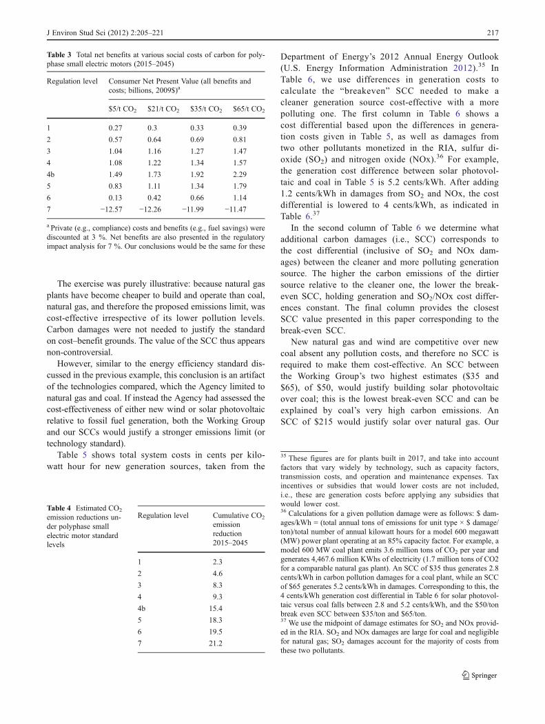
The exercise was purely illustrative: because natural gasplants have become cheaper to build and operate than coal,natural gas, and therefore the proposed emissions limit, wascost-effective irrespective of its lower pollution levels.Carbon damages were not needed to justify the standardon cost–benefit grounds. The value of the SCC thus appearsnon-controversial.

However, similar to the energy efficiency standard dis-cussed in the previous example, this conclusion is an artifactof the technologies compared, which the Agency limited tonatural gas and coal. If instead the Agency had assessed thecost-effectiveness of either new wind or solar photovoltaicrelative to fossil fuel generation, both the Working Groupand our SCCs would justify a stronger emissions limit (ortechnology standard).

Table 5 shows total system costs in cents per kilo-watt hour for new generation sources, taken from the

Department of Energy’s 2012 Annual Energy Outlook(U.S. Energy Information Administration 2012).35 InTable 6, we use differences in generation costs tocalculate the “breakeven” SCC needed to make acleaner generation source cost-effective with a morepolluting one. The first column in Table 6 shows acost differential based upon the differences in genera-tion costs given in Table 5, as well as damages fromtwo other pollutants monetized in the RIA, sulfur di-oxide (SO2) and nitrogen oxide (NOx).36 For example,the generation cost difference between solar photovol-taic and coal in Table 5 is 5.2 cents/kWh. After adding1.2 cents/kWh in damages from SO2 and NOx, the costdifferential is lowered to 4 cents/kWh, as indicated inTable 6.37

In the second column of Table 6 we determine whatadditional carbon damages (i.e., SCC) corresponds tothe cost differential (inclusive of SO2 and NOx dam-ages) between the cleaner and more polluting generationsource. The higher the carbon emissions of the dirtiersource relative to the cleaner one, the lower the break-even SCC, holding generation and SO2/NOx cost differ-ences constant. The final column provides the closestSCC value presented in this paper corresponding to thebreak-even SCC.

New natural gas and wind are competitive over newcoal absent any pollution costs, and therefore no SCC isrequired to make them cost-effective. An SCC betweenthe Working Group’s two highest estimates ($35 and$65), of $50, would justify building solar photovoltaicover coal; this is the lowest break-even SCC and can beexplained by coal’s very high carbon emissions. AnSCC of $215 would justify solar over natural gas. Our

Table 4 Estimated CO2

emission reductions un-der polyphase smallelectric motor standardlevels

Regulation level Cumulative CO2

emissionreduction2015–2045

1 2.3

2 4.6

3 8.3

4 9.3

4b 15.4

5 18.3

6 19.5

7 21.2

36 Calculations for a given pollution damage were as follows: $ dam-ages/kWh = (total annual tons of emissions for unit type × $ damage/ton)/total number of annual kilowatt hours for a model 600 megawatt(MW) power plant operating at an 85% capacity factor. For example, amodel 600 MW coal plant emits 3.6 million tons of CO2 per year andgenerates 4,467.6 million KWhs of electricity (1.7 million tons of CO2for a comparable natural gas plant). An SCC of $35 thus generates 2.8cents/kWh in carbon pollution damages for a coal plant, while an SCCof $65 generates 5.2 cents/kWh in damages. Corresponding to this, the4 cents/kWh generation cost differential in Table 6 for solar photovol-taic versus coal falls between 2.8 and 5.2 cents/kWh, and the $50/tonbreak even SCC between $35/ton and $65/ton.37 We use the midpoint of damage estimates for SO2 and NOx provid-ed in the RIA. SO2 and NOx damages are large for coal and negligiblefor natural gas; SO2 damages account for the majority of costs fromthese two pollutants.

Table 3 Total net benefits at various social costs of carbon for poly-phase small electric motors (2015–2045)

Regulation level Consumer Net Present Value (all benefits andcosts; billions, 2009$)a

$5/t CO2 $21/t CO2 $35/t CO2 $65/t CO2

1 0.27 0.3 0.33 0.39

2 0.57 0.64 0.69 0.81

3 1.04 1.16 1.27 1.47

4 1.08 1.22 1.34 1.57

4b 1.49 1.73 1.92 2.29

5 0.83 1.11 1.34 1.79

6 0.13 0.42 0.66 1.14

7 −12.57 −12.26 −11.99 −11.47

a Private (e.g., compliance) costs and benefits (e.g., fuel savings) werediscounted at 3 %. Net benefits are also presented in the regulatoryimpact analysis for 7 %. Our conclusions would be the same for these

35 These figures are for plants built in 2017, and take into accountfactors that vary widely by technology, such as capacity factors,transmission costs, and operation and maintenance expenses. Taxincentives or subsidies that would lower costs are not included,i.e., these are generation costs before applying any subsidies thatwould lower cost.


closest corresponding SCC is the 99th percentile using a 2.5%discount rate, $221. Wind would require an SCC of $74 to becost-effective over natural gas. This is slightly above theWorking Group’s highest SCC ($65), but significantly belowour next highest estimate of $107 (95th percentile estimateusing a 2.5 % discount rate).

The break-even SCCs presented here are conservativein three respects. First, the SCC grows over time,whereas the SCCs used here are for 2010.38

Accounting for the growth of SCCs over time wouldincrease the cost of generation (inclusive of carbondamages) with coal or gas for a given starting SCC,reducing the 2010 SCC that corresponds to break evengeneration costs. Second, technological innovation maycontinue to drive down costs of wind and solar in thefuture, further lowering the break-even SCC. Third, wedo not account for externalities other than air emissionsfrom the power plants, such as methane emissions fromnatural gas wells and land disturbance from coalmining.

Discussion

These two regulatory impact analyses suggest that over-all emission reductions achieved by a collection ofefficiency and air pollution standards could be influ-enced by the SCC. This appears to be the case withthe Working Group’s higher SCCs, and even more sowith our alternative SCCs (or if the SCC increases forother reasons). Executive orders emphasizing the impor-tance of benefits relative to costs are not legally bind-ing, but regulators may feel more comfortable proposingstricter rules the more they can back them up withstrong benefits calculations.

Recent Congressional attacks on the Clean Air Actare instructive: advocates have vigorously defended theAct by pointing to the enormous benefit–cost ratiosfound in EPA’s economic analyses of the statute’s im-plementation, and these ratios are frequently cited in the

press.39 Interestingly, one monetized benefit drives thisresult: the value of reducing risks to life, as measuredby the “value of a statistical life” (VSL).40 Estimates ofthe VSL started out very small, but grew substantiallyover time as they developed in the economics litera-ture.41 If SCC estimates follow the same trajectory, thelong-run consequence of its role in cost–benefit analysiscould be significant. Stronger standards might be pro-posed, and those that are promulgated are likely to beeasier to defend against political attacks.

Conclusion

Regulatory standards governing carbon emission reductionsmay well hinge on the value of the social cost of carbon(SCC). The estimates we report under our different sensitivi-ties span values that are markedly higher than the WorkingGroup‘s. Had the Working Group used a set of discount ratesand discounting methodology considered appropriate for in-tergenerational costs and benefits, more stringent standardswould be justified. The same conclusion applies to our equityweighting results: had the Working Group weighed damagesaccording to income levels, a common practice in the SCCliterature, its values would be much higher. Even net benefitscalculations using the Working Group’s own range of valuescan justify higher stringency levels, depending upon which oftheir SCCs are used.

In addition to demonstrating the importance of discountingand equity weighting on the Working Group’s estimates, wehope we have provided a useful introduction to the social costof carbon. Its estimation is a fundamentally interdisciplinaryexercise involving multiple ethical and technical challenges;improving upon it thus depends critically upon input from a

Table 5 Generationcosts for new plantsconstructed in 2017

Cents/kWh (2007$)

Natural gas 6.3

Wind 9.1

Coal 9.3

Solarphotovoltaic

14.5

39 Benefits of the 1990 amendments to the Clean Air Act (CAA) areestimated to exceed costs by a ratio of 26 to 1 in 2010, and 30 to 1 in2020 (EPA 2011).40 EPA summarizes this measure as follows: “[W]hen conducting abenefit–cost analysis of new environmental policies, the Agency usesestimates of how much people are willing to pay for small reductions intheir risks of dying from adverse health conditions that may be caused byenvironmental pollution…This is best explained by way of an example.Suppose each person in a sample of 100,000 people were asked howmuch he or she would be willing to pay for a reduction in their individualrisk of dying of 1 in 100,000, or 0.001 %…[if the average willingness topay for this reduction in risk were $100] [t]hen the total dollar amount…to save one statistical life in a year would be $100 per person×100,000people, or $10 million” (http://yosemite.epa.gov/ee/epa/eed.nsf/pages/MortalityRiskValuation.html#whatisvsl).41 Early economic theory estimated the value of a life usingforegone earnings (i.e., the value of a lost life was equal to theindividual’s remaining lifetime earnings), which produced esti-mates far lower than today’s that use VSL methodology. EPAcurrently uses $7.6 million per life. (http://yosemite.epa.gov/ee/epa/eed.nsf/pages/MortalityRiskValuation.html#whatvalue, con-verted from 2006$ to 2007$).

38 The SCC increases over time because future emissions are expectedto produce larger incremental damages as physical and economicsystems become more stressed in response to greater climatic change.


http://yosemite.epa.gov/ee/epa/eed.nsf/pages/MortalityRiskValuation.html#whatisvsl

http://yosemite.epa.gov/ee/epa/eed.nsf/pages/MortalityRiskValuation.html#whatisvsl

http://yosemite.epa.gov/ee/epa/eed.nsf/pages/MortalityRiskValuation.html#whatvalue

http://yosemite.epa.gov/ee/epa/eed.nsf/pages/MortalityRiskValuation.html#whatvalue

broad range of expertise. With the unlikely prospect of com-prehensive climate legislation in Congress at present, direct orindirect (e.g., through energy efficiency standards) regulationof greenhouse gases under existing law is likely to be theprimary tool used to address climate change in the UnitedStates for the foreseeable future, with the SCC taking on anincreasingly important role.

Acknowledgments The authors would like to thank David Anthoff,Blair Beasley, Dallas Burtraw, Dan Lashof, Antony Millner, and severalanonymous reviewers for their helpful comments. Any errors are our own.

Appendix

The FUND model uses the Ramsey discounting formula toapply regional equity weights to damages based uponwhether they occur in poorer versus wealthier regions.

To understand the methodology in more detail, thisAppendix describes the discounting equations them-selves—both the one used by the Working Group, andthe Ramsey formulation we used to apply regional eq-uity weights. We include here a review of some of theconcepts discussed in “The social cost of carbon modelsused by the Working Group” section.

Equation 1 below shows the Working Group’s discountrate formula, where δ is the constant discount rate, t the timeperiod, r a given region, and Dtr damages in region r in timeperiod t caused by one additional ton of CO2 emitted today.T is the number of years considered for the analysis.

SCC with constant discounting dð Þ¼ P

r

PT

t¼0Dtr

11þd

� �t¼ PT

t¼0

11þd

� �t P

rDtr

ð1Þ

In layman’s terms, Eq. 1 discounts all damages by thesame discount rate δ, regardless of the region in which theyoccur, and then sums them over time.

Equation 2 describes Ramsey discounting, without anequity weight applied between regions.

SCC with Ramsey discounting without regional equity weights ρ; η; gtð Þ¼ P

r

PT

t¼0Dtr

1

1þ ρþ ηgt

� �t

|fflfflfflfflfflfflfflfflfflfflfflffl{zfflfflfflfflfflfflfflfflfflfflfflffl}Ramsey discount

factor

ð2Þ

where η is the elasticity of marginal utility, ρ the pure rate oftime preference (PRTP), and gt average per capita worldconsumption growth between the present and time t.42 ThePRTP is the most controversial parameter, as it captures atendency to prefer experiencing utility from consumptiontoday rather than delaying it into the future—thus discount-ing future damages to individuals simply because they havethe misfortune of being born later. The parameter η repre-sents the idea that as one’s income increases, each additionaldollar brings less utility; correspondingly, one dollar’s worthof climate damages causes more “disutility” to a poor indi-vidual than it does to a wealthier one. The growth term, gt,correspondingly captures changes in income. If gt is posi-tive, the discount rate increases; if it is negative, it decreases.

Finally, we apply a regional equity weight to Eq. 2

SCC ¼X

r

Cn

C0r

� �

|fflfflffl{zfflfflffl}equityweight

η XT

t¼0Dtr

1

1þ ρþ ηgtr

� �t

|fflfflfflfflfflfflfflfflfflfflfflffl{zfflfflfflfflfflfflfflfflfflfflfflffl}Ramsey discount

factor

�X

r

XT

t¼0Dtr

Cn

Ctr

� �η 1

1þ ρ

� �t

ð3Þ

where Cn is consumption per capita in time 0 in the region towhich other regions’ damages are weighted, Cor per capita

42 More precisely, let gs be the actual consumption growth rate at time

s, then gt is defined by the following equation 1þ gtð Þ�t ¼ Qts¼0

1þ gsð Þ�1 , i.e., gt is the geometric mean growth from the present totime t.

Table 6 SCCs required to make cleaner generation cost-effective (2007$)

Cost differential for cleaner sourceto be cost-effective (cents/kWh),excluding carbon

Break-even2010 SCC

Closest Working Group (WG) and/orJohnson-Hope (JH) cost-effective SCC

Natural gas versus coal Not applicable* Not applicable* Not applicable*

Wind versus coal Not applicable* Not applicable* Not applicable*

Solar photovoltaic versus coal 4 $50 Between WG 2.5 % ($35) and WG3 % 95th percentile ($65)

Wind versus natural gas 2.8 $74 Between WG 3 % 95th percentile ($65)and JH 2.5 % 95th percentile ($107)**

Solar photovoltaic versus natural gas 8.2 $215 JH 2.5 % 99th percentile ($221)**

*Both natural gas and wind are more cost-effective than coal without consideration of carbon damages.

**Even though the Working Group uses 2.5 percent as one of its discount rates, we classify this as a JH estimate because the Working Group doesnot include this value as one that regulatory agencies can use in their impact analyses


consumption at time 0 for a given region r for which theequity weight is computed, and Ctr per capita consumptionat time t in region r. gtr now stands for the average con-sumption growth between the present and time t in region r(the precise definition follows the same method as outlinedin the footnote above).

We set Cn equal to U.S. per capita income, so that theequity weight for impacts in the U.S.A. is 1, i.e., thatimpacts in the U.S.A. are valued the same way as any othercost or benefit within the U.S.A. would be valued.43,44

To estimate a regionally equity weighted SCCcorresponding to a given constant consumption discountrate used by the Working Group, we first solved for thevalue of ρ in Eq. 2 that gave us the same SCC as obtainedfor a given consumption discount rate δ in Eq. 1, assuming avalue of 1 for η and the realized consumption growth ratescorresponding to the given EMF-22 socioeconomic scenariofor different regions. For each EMF-22 scenario, weobtained a value for ρ, denoted hereafter ρ. After solvingfor ρ, we then substituted that value into Eq. 3, to get thefinal regionally equity weighted SCCs corresponding to thedifferent consumption discount rates. In effect, we isolatethe impact of adding equity weights from the time discount-ing component of the Working Group’s SCCs.

We set η equal to 1 because it was the simplest way to dothe calculation, and because it is the most used value in theliterature. It is important to note, however, that in thisexercise we are not advocating any particular value of η(or ρ); rather, we are demonstrating the importance of im-posing regional equity weights on the Working Group’sSCC estimates for a given consumption discount rate.

Different values of η would produce different SCCs andcorresponding ρ s , so the equity-weighted estimates pre-sented here should not be interpreted as the only possiblevalues the Working Group would have obtained had it usedregional equity weights. In general, damages can increase ordecrease as η increases, depending upon how incomes forrich versus poor regions compare relative to one another in agiven time period (equity weighting between regions in agiven time period), and relative to their starting values(“marginal utility” weighting for a given region over timevia the discount rate). The latter effect, however, does notimpact our SCCs, as we held that constant by varying ρ (seeabove). The effect of η can also vary depending uponwhether regions are assumed to get benefits from climatechange (e.g., through CO2 fertilization) and the income levelof regions obtaining such benefits.

References

Ackerman F, Stanton EA (2011) Climate economics: the state of theart. Stockholm Environment Institute—U.S. Center, Summerville,MA

Ackerman F, Stanton EA, Hope C, Alberth S (2009) Did the SternReview underestimate US and global climate damages? EnergyPolicy 37(7):2717–2721

Anthoff D, Hepburn C, Tol R (2009) Equity weighting and the mar-ginal damage costs of climate change. Ecol Econ 68(3):836–849

Arrow K (2000) A comment on cooper. The World Bank ResearchObserver 15(2)

Azar C, Sterner T (1996) Discounting and distributional considerationsin the context of global warming. Ecol Econ 19(2):169–184

Arrow KJ, Cline WR, Maler KG, Munasinghe M, Squitieri R, StiglitzJE (1996) Intertemporal equity, discounting, and economic effi-ciency. In: Bruce JP, Lee H, Haites EF (eds) Climate Change1995: Economic and Social Dimensions of Climate Change.Cambridge University Press, Boston, MA

Clarkson R, Deyes K (2002) Estimating the social cost of carbonemissions. Government Economics Service Working Paper. HMTreasury, London

Cochrane JH (2001) Asset pricing. Princeton University Press,Princeton

Daly H, Cobb J (1989) For the common good. Beacon, BostonDietz S, Hepburn C, Stern N (2009) Economics, ethics and climate

change. In: Basu K, Kanbur R (eds) Arguments for a better world:essays in Honour of Amartya Sen (volume 2: Society Institutionsand Development). Oxford University Press, Oxford

Fankhauser S, Tol R, Pearce DW (1997) The aggregation of climatechange damages: a welfare theoretic approach. Environ ResourEcon 10(3):249–266

Fisher A, Hanemann M, Roberts M, Schlenker W (2012) The econom-ic impacts of climate change: evidence from agricultural outputand random fluctuations in weather: comment. American Eco-nomic Review

Goodstein ES (2004) Economics and the environment, 3rd edn. Hobo-ken, NJ, Wiley

Hope C (2006) The marginal impact of CO2 from PAGE2002: anintegrated assessment model incorporating the IPCC’s fivereasons for concern. The Integrated Assessment Journal 6(1):19–56

43 Ideally, the models would be constructed at a more disaggregatedlevel such that inequalities within countries could also be accountedfor. At present, however, the models are not sufficiently developed todo so, and it would be challenging to modify them due to limitedinequality data in many parts of the world.44 It is important to note that equity weighted results can be presentedusing different per capita consumption levels for normalization, as longas the costs of mitigation (and any other costs and benefits in the U.S.)are similarly weighted. Regardless of the normalization weight chosen,if it is consistently applied across all costs and benefits the conclusionof a cost–benefit analysis will not change (i.e., the cost–benefit ratiowill stay the same). In calculating an SCC for any given region, usingthat region’s per capita income as the normalization weight reduces thelikelihood of errors in a cost–benefit analysis. If a social cost of carbonthat is equity weighted and normalized with world average per capitaconsumption is used in a U.S. cost–benefit analysis, one consequentlyhas to equity weight the other costs and benefits the same way, with aweight also less than 1. In practice this would be highly cumbersome,confusing, and prone to error. Alternatively one can pick U.S. percapita income as the normalization for the equity weighting, as wasdone in Anthoff et al. (2009) and for the FUND results presented in thispaper. With this normalization, the equity weight for the U.S. is 1, andthe need to equity weight any other costs or benefits in the U.S. towhich the benefits of emission reductions might be compared is notnecessary, given that a weight of 1 would not change these estimates.


Hope C (2008) Optimal carbon emissions and the social cost of carbonunder uncertainty. The Integrated Assessment Journal 8(1):107–122

Howarth RB (2003) Discounting and uncertainty in climate changepolicy analysis. Land Economics 79(3):369–381

Ibbotson Associates (2001) Stocks, bonds, and inflation. IbbotsonAssociates, Chicago

Intergovernmental Panel on Climate Change (2007) Fourth Assess-ment Report Climate Change

Kousky C, Kopp RE (2011) Risk premia and the social cost of carbon: areview. Economics: The Open-Access, Open-Assessment E-Journal.Discussion Paper No. 2011-19. http://www.economics-ejournal.org/economics/discussionpapers/2011-19

Le Treut HR, Somerville I, Cubasch Y, Ding C, Mauritzen A, Mokssit,Peterson T, Prather M (2007). Historical overview of climatechange. In: Solomon S, Qin D, Manning M, Chen Z, MarquisM, Averyt KB, Tignor M, Miller HL (eds) Climate change 2007:the physical science basis. Contribution of Working Group I to theFourth Assessment Report of the Intergovernmental Panel onClimate Change. Cambridge University Press, Cambridge

Lobell D, Schlenker W, Costa-Roberts J (2011) Climate trends andglobal crop production since 1980. Science 333(6042):616–620

Lowe J (2008) Intergenerational wealth transfers and social discount-ing: supplementary greenbook guidance. UK Treasury. http://www.hm-treasury.gov.uk/d/4(5).pdf

Mastrandrea M (2009) Calculating the benefits of climate policy:examining the assumptions of Integrated Assessment Models.Pew Center on Global Climate Change Working Paper

Masur JS, Posner EA (2010) Climate regulation and the limits of cost–benefit analysis. John M. Olin Law & Economics Working PaperNo. 525 and Public Law and Legal Theory Working Paper No. 315

Newell R, Pizer W (2003) Discounting the distant future: how much douncertain rates increase valuations? J Environ Econ Manag46:52–71

Nordhaus W (2008) A question of balance: weighing the options onglobal warming policies. Yale University Press, Princeton, NJ

Nordhaus W (2011) Estimates of the social cost of carbon: backgroundand results from the RICE-2011 model. Cowles Foundation Dis-cussion Paper No. 1826

Nordhaus W, Boyer J (2000) Warming the world: economic models ofglobal warming. MIT Press, Cambridge, MA

Nordhaus W, Tobin J (1972) Is growth obsolete? In Economic re-search: retrospect and prospect Vol 5: Economic Growth, NationalBureau of Economic Research

Ramsey F (1928) A mathematical theory of saving. Econ J 38:543–559Roberts M, Schlenker W (2012) Is agricultural production becoming

more or less sensitive to extreme heat? Evidence from U.S. cornand soybean yields. In: Fullerton D, Catherine, W (eds) TheDesign and Implementation of U.S. Climate Policy. Universityof Chicago Press, Chicago

Roe G, Baker M (2007) Why is climate sensitivity so unpredictable?Science 318:629

Schlenker W, Roberts M (2009) Nonlinear temperature effects indicatesevere damages to U.S. crop yields under climate change. Proceed-ings of the National Academy of Sciences 106(37):15594–15598

Stern N (2007) The Stern Review: the economics of climatechange. Cambridge, UK: Cambridge University Press, availableonline at http://www.hm-treasury.gov.uk/independent_reviews/stern_review_economics_climate_change/sternreview_index.cfm

Sterner T, Persson UM (2008). An even sterner review: introducingrelative prices into the discounting debate. Review of Environ-mental Economics and Policy 2(1):61–76

Talberth J, Cobb J, Slattery N (2007) The genuine progress indicator2006: a tool for sustainable development. Redefining progress,Oakland, CA

Tol R (2002a) Estimates of the damage costs of climate change. Part I:benchmark estimates. Environmental and Resource Economics21:47–73

Tol R (2002b) Estimates of the damage costs of climate change. Part II:dynamic estimates. Environmental and Resource Economics21:135–160

Tol R (2009) An analysis of mitigation as a response to climate change.Copenhagen Consensus on Climate. Discussion Paper

Umweltbundesamt (2007) Okonomisch Bewertung von Umweltscha-den: Methodenkonvention zur Schantzun externer Umweltkosten.Dessau

U.S. Department of Energy (2010) Energy conservation program:energy conservation standards for small electric motors. FedRegist 75:10874–10948

U.S. Energy Information Administration (2012) Levelized cost ofnew generation resources in the Annual Energy Outlook2012. USEIA, Washington DC. www.eia.gov/forecasts/aeo/electricity_generation.cfm

U.S. Environmental Protection Agency (2008) Technical support doc-ument on benefits of reducing GHG emissions. USEPA, Wash-ington DC

U.S. Environmental Protection Agency (2011) The benefits and costsof the Clean Air Act from 1990 to 2020. USEPA, Washinton DC

U.S. Environmental Protection Agency (2012) Standards of perfor-mance for greenhouse gas emissions for stationary sources; elec-tricity utility generating units. Fed Regist 72:22392–22441

U.S. Government (2010) Interagency Working Group on Social Costof Carbon. Technical support document: social cost of carbon forregulatory impact analysis under Executive Order 12866

U.S. Office of Management and Budget (September 17, 2003) Regu-latory analysis (OMB Circular A-4)

Weitzman M (2001) Gamma discounting. Am Econ Rev 91(1):260–271Zolatas X (1981) Economic growth and declining social welfare. New

York University Press, New York


http://www.economics-ejournal.org/economics/discussionpapers/2011-19

http://www.economics-ejournal.org/economics/discussionpapers/2011-19

http://www.hm-treasury.gov.uk/d/4(5).pdf

http://www.hm-treasury.gov.uk/d/4(5).pdf

http://www.hm-treasury.gov.uk/independent_reviews/stern_review_economics_climate_change/sternreview_index.cfm

http://www.hm-treasury.gov.uk/independent_reviews/stern_review_economics_climate_change/sternreview_index.cfm

http://www.eia.gov/forecasts/aeo/electricity_generation.cfm

http://www.eia.gov/forecasts/aeo/electricity_generation.cfm

Documents

Natural Resources Defense Council Appliance Standards