Embed Size (px)
Citation preview

Doney et al., Natural Climate-Carbon Cycle Variability, J. Climate, submitted.
1
Natural Variability in a Stable, 1000 Year Global CoupledClimate-Carbon Cycle Simulation
Journal of ClimateSubmitted: June 17th, 2005Revised: October 31st, 2005
Scott C. DoneyMarine Chemistry and GeochemistryWoods Hole Oceanographic InstitutionWoods Hole, MA 02543, [email protected]
Keith LindsayClimate and Global DynamicsNational Center for Atmospheric ResearchBoulder, CO 80307, USA
Inez Fung and Jasmin JohnBerkeley Atmospheric Sciences CenterUniversity of California, BerkeleyBerkeley, CA 94720, USA

Doney et al., Natural Climate-Carbon Cycle Variability, J. Climate, submitted.
2
Abstract
A new three-dimensional global coupled carbon-climate model is presented in the
framework of the Community Climate System Model (CSM-1.4). The biogeochemical
module includes explicit land water-carbon coupling, dynamic carbon allocation to leaf,
root and wood, prognostic leaf phenology, multiple soil and detrital carbon pools, oceanic
iron limitation, a full ocean iron cycle, and 3-D atmospheric CO2 transport. A sequential
spin-up strategy is utilized to minimize the coupling shock and drifts in land and ocean
carbon inventories. A stable, 1000-year control simulation-global annual mean surface
temperature ±0.10 K and atmospheric CO2 ±1.2 ppm (1σ)-is presented with no flux
adjustment in either physics or biogeochemistry. The control simulation compares
reasonably well against observations for key annual mean and seasonal carbon cycle
metrics; regional biases in coupled model physics, however, propagate clearly into
biogeochemical error patterns. Simulated interannual to centennial variability in
atmospheric CO2 is dominated by terrestrial carbon flux variability, ±0.69 Pg C y-1 (1σ ,
global net annual mean), which in turn reflects primarily regional changes in net primary
production modulated by moisture stress. Power spectra of global CO2 fluxes are white
on timescales beyond a few years, and thus most of the variance is concentrated at high
frequencies (timescale < 4 years). Model variability in air-sea CO2 fluxes, ±0.10 Pg C y-1
(1σ , global annual mean), is generated by variability in sea surface temperature, wind
speed, export production, and mixing/upwelling. At low frequencies (timescale > 20
years), global net ocean CO2 flux is strongly anti-correlated (0.7 to 0.95) with the net CO2
flux from land; the ocean tends to damp (20-25%) slow variations in atmospheric CO2

Doney et al., Natural Climate-Carbon Cycle Variability, J. Climate, submitted.
3
generated by the terrestrial biosphere. The intrinsic, unforced natural variability in land
and ocean carbon storage is the “noise” that complicates the detection and mechanistic
attribution of contemporary anthropogenic carbon sinks.
(1) Introduction
Over the last two centuries, the levels of atmospheric carbon dioxide CO2, an
important greenhouse gas that modulates Earth’s radiative balance and climate, have
increased due to fossil-fuel combustion and land-use. Levels have risen from a
preindustrial value of 280 ppm to about 380 ppm at present, equivalent to an increase of
~200 Pg of carbon (1 Pg =1015g) (Prentice et al., 2001). By comparison, atmospheric
carbon dioxide levels for the preceding several millennia of the Holocene were
essentially flat, within plus or minus 5 ppm of the preindustrial value. ‘Business as usual’
economic and climate scenarios project values as high as 700 to 1000 ppm by the end of
the twenty-first century, levels not experienced on Earth for the past several million years
(Pearson and Palmer, 2000). There is growing evidence that this increase in atmospheric
CO2 will have a significant, long-term impact on the planet’s climate and biota (IPCC,
2001).
Recent estimates suggest that only about half of the fossil fuel CO2 released by
human activity during the last two decades has remained in the atmosphere; on average,
about equal amounts or roughly 2 Pg C/yr have been taken up by the ocean and land,
respectively. As global climate models are improved, the future behavior of these land
and ocean carbon sinks and the resulting atmospheric forcing are emerging as one of the

Doney et al., Natural Climate-Carbon Cycle Variability, J. Climate, submitted.
4
main uncertainties associated with climate projections (Hansen et al., 1998; Prentice et
al., 2001). In most previous anthropogenic climate change projections, the trajectory of
atmospheric CO2 concentration is prescribed and the resulting physical climate response
computed. This approach, however, neglects the potential for substantial feedbacks
between climate change and the carbon cycle that could either exacerbate or partially
ameliorate global climate change.
Human perturbations to the Earth’s climate occur on top of a large natural carbon
cycle, a complex system involving the ocean, atmosphere and land domains and the
fluxes among them. Many of the underlying ecological and biogeochemical processes are
sensitive to shifts in temperature, the hydrological cycle, and ocean dynamics, and the
magnitude and, in some cases, even the sign of specific carbon-climate feedbacks are
unknown. Two recent studies by Cox et al. (2000) and Dufresne et al. (2002) present
strikingly different pictures of carbon-climate feedbacks, differences that must arise
because of the underlying formulations linking the physical climate and biogeochemistry.
On geological time-scales, ice core and other paleo-proxy reconstructions suggest large
contemporaneous variations in climate and atmospheric CO2, ranging from glacial-
interglacial cycles (Petit et al., 1999) to the high CO2, warm periods of the Cretaceous
and Permian; the exact interplay of climate forcing and carbon cycle dynamics on these
scales also is not well resolved.
Numerical models provide one of the few direct and quantitative methods for
assessing such questions, and a number of recent studies have explored the behavior of

Doney et al., Natural Climate-Carbon Cycle Variability, J. Climate, submitted.
5
coupled carbon-climate simulations (Friedlingstein et al., 2001; Thompson et al., 2004l
Zeng et al., 2004; Mathews et al., 2005; Govindasamy et al., 2005). Here we present a
new, fully coupled 3-D climate-carbon cycle model based on the framework of the
Community Climate System Model (CCSM) project (Blackmon et al., 2001). The overall
objectives of the CCSM-carbon project are to better understand: (1) what processes and
feedbacks are most important in setting atmospheric CO2, and (2) how do CO2 and
climate co-evolve. We focus in this paper on the description of the land, ocean and
atmosphere biogeochemical component models (Section 2), their integration within the
CSM 1.4 physical model framework, and the analysis of a stable, 1000-year pre-
industrial simulation. By introducing a sequential spin-up procedure, we minimize the
drifts in land and ocean carbon inventories that can arise from biases in coupled model
physical climate (Section 3). In Section 4, we assess the skill of the control simulation by
comparing the annual mean and seasonal cycle of key simulated carbon metrics against
observations. We fully resolve the 3-D structure of atmospheric CO2, providing important
constraints on model dynamics. We then use the control integration to quantify the
magnitude and physical mechanisms of natural interannual, decadal, and centennial
variability in carbon exchange within and among the reservoirs (Section 5).
The simulations presented here focus on carbon cycle responses to intrinsic,
natural variability of the physical climate system. We do not include here natural external
climate perturbations such as volcanic eruptions and solar variability that may impact
carbon cycle variability (e.g., Gerber et al., 2003; Trudinger et al., 2005). Experiments
using the CSM 1-Carbon model exploring the carbon-climate feedbacks arising from the

Doney et al., Natural Climate-Carbon Cycle Variability, J. Climate, submitted.
6
anthropogenic fossil fuel CO2 emissions for the 19th, 20th, and 21st centuries are presented
in Fung et al. (2005). Key finds reported there include: an inverse relationship between
carbon sink strengths and the rate of fossil fuel emissions; a positive carbon-climate
feedback where climate warming increases atmospheric CO2 and amplifies the climate
change; and large regional changes in terrestrial carbon storage modulated by hydrologic
and ecosystem responses.
(2) Model Description
The coupled carbon-climate model treats radiative CO2 as a prognostic variable,
with the atmospheric abundance as the residual after accounting for the climate-sensitive
fluxes into and out the land biosphere (Fab and Fba, respectively), and into and out of the
ocean (Fao and Foa, respectively).
oaaobaab FFFFurceExternalSoCOCOt
+−+−=ℑ+∂∂
)( 22 (1)
In Equation 1,
€
ℑ(CO2) is the 3-dimensional atmospheric transport of CO2 due to large-
scale advection and to turbulent mixing associated with dry and moist convection. We
have added Equation 1 to the NCAR coupled atmosphere-land-ocean-ice physical climate
model (CSM 1.4) and embedded new versions of a terrestrial carbon module to estimate
Fab and Fba, and oceanic carbon module to estimate Fao and Foa . These are described
below. In the control run described here, ExternalSource=0. The CSM 1.4-Carbon

Doney et al., Natural Climate-Carbon Cycle Variability, J. Climate, submitted.
7
source code and the simulations discussed here are electronically available from:
http://www.ccsm.ucar.edu/working_groups/Biogeo/csm1_bgc/
(2.1) CSM 1.4 coupled physical model
The core of the coupled carbon-climate model is a modified version of NCAR
CSM1.4, consisting of ocean, atmosphere, land, and sea-ice physical components
integrated via a flux coupler (Boville and Gent, 1998; Boville et al., 2001). The
simulations here are integrated with an atmospheric spectral truncation resolution of T31
(~3.75°) with 18 levels in the vertical, and an ocean resolution of 3.6° in longitude and
0.8° to 1.8° latitude and 25 levels in the vertical (referred to as T31x3). The sea ice
component model runs at the same resolution as the ocean model, and the land surface
model runs at the same resolution as the atmospheric model. Physical control simulations
display stable surface temperatures and minimal deep ocean drift without requiring
surface heat or freshwater flux adjustments. The water cycle is closed through a river
runoff scheme, and modifications have been made to the ocean horizontal and vertical
diffusivities and viscosities from the original version (CSM 1.0) to improve the equatorial
ocean circulation and interannual variability.
The 3-D atmospheric CO2 distribution is advected and mixed as a dry-air mixing
ratio using a semi-Lagrangian advection scheme; both dry and moist turbulent mixing
schemes are used for the transport of water vapor mass fractions. The model CO2 field
affects the shortwave and longwave radiative fluxes through the column average CO2
concentration.

Doney et al., Natural Climate-Carbon Cycle Variability, J. Climate, submitted.
8
(2.2) Land carbon-cycle model
The CSM1.4-carbon land carbon module (Figure 1) combines the NCAR Land
Surface Model (LSM) biogeophysics package (Bonan, 1996) with the Carnegie-Ames-
Stanford Approach (CASA) biogeochemical model (see Randerson et al., 1997). Both the
LSM and CASA models are documented extensively in the literature. Here we provide a
brief overview of the models and highlight changes that have been made to the standard
model dynamics. The land surface is characterized by the fractional coverage of 14 plant
functional types (PFTs) and 3 soil textures (Bonan 1996). LSM estimates leaf-level
stomatal conductance of CO2 and water to maximize carbon assimilation for sunlit and
shady conditions (Collatz et al. 1990; Sellers et al. 1996). The carbon assimilation is
integrated through the canopy using the fraction of sun-lit and shade leaves to yield gross
primary productivity (GPP). A terrestrial CO2 fertilization effect arises physiologically in
the model because carbon assimilation via the Rubisco enzyme is limited by internal leaf
CO2 concentrations; GPP thus increases with external atmospheric CO2 concentrations,
eventually saturating at high CO2 levels.
In this implementation, net primary productivity (NPP = Fab) is assumed to be
50% of GPP calculated by LSM (replacing NPP calculated by CASA). The NPP/GPP
ratio has been demonstrated to be constant on annual time scales across a wide range of
forests (Waring et al. 1998). While it is well-known that autotrophic respiration (Ra)
varies seasonally and diurnally, we have not modeled Ra explicitly, as its magnitude as
well as sensitivity to temperature and other control variables remain uncertain even in
high-frequency flux tower measurements (e.g. Wohlfahrt et al., 2005; Reichstein et al.

Doney et al., Natural Climate-Carbon Cycle Variability, J. Climate, submitted.
9
2005). The impact of this assumption on modeled CO2 cannot be readily quantified, as
global-scale constraints are available for the seasonal variability of NPP (via satellite
observations of the NDVI) and on the net flux (via the seasonal oscillations of
atmospheric CO2), and not for GPP or respiration.
NPP is allocated to three live biomass pools M (leaf, wood, root) following
Friedlingstein et al. (1999), with preferred allocation to roots during water-limited
conditions and to leaves during light-limited conditions:
k
kkk
MNPPM
t τα −=
∂
∂k=1,2,3 (2)
In the CASA formulation, turnover times τk of the three live pools are PFT-specific but
time-invariant, with constants ranging from 1.8 years for leaves in tropical broadleaved
evergreen trees to 48 years for wood in broadleaf deciduous tress. The leaf mortality of
deciduous trees is modified to include cold-drought stress to effect leaf-fall in 1-2
months, and leaf biomass (kgC/m2 land) is translated into prognostic leaf area indicies
(LAI) using specific leaf areas (SLA, m2 leaf /kgC), following Dickinson et al. (1998), so
that LAI varies with climate. We place limits on LAI, with a minimum of 0.6 to simulate
the storage of carbon in photosynthates and a maximum of 6 to simulate light and
nutrient limitation. The excess carbon above the maximum Mleaf is added to litterfall
Mleaf/τleaf.
There are 9 dead carbon pools, with leaf mortality contributing to metabolic and
structure surface litter (k=4,5), root mortality contributing to metabolic and structure soil
litter (k=6,7), and wood mortality contributing to coarse woody debris (CWD, k=8). The

Doney et al., Natural Climate-Carbon Cycle Variability, J. Climate, submitted.
10
subsequent decomposition of Mk, k=4-8 by microbes leads to transfer of carbon to the
dead surface and soil microbial pools (k=9,10) and the slow and passive pools (k=11,12).
A fraction of each carbon transfer is released to the atmosphere via microbial or
heterotrophic respiration. This is summarized in Equation 3:
k
k
nkn
n k
kkn
j j
jjkk
MMMMt τ
γτ
γτ
γ )1(12
4
12
4
12
1∑∑∑===
−−−=∂∂
k=4,…12 (3)
The first term on the RHS of Equation 3 is the gain of Mk due to litterfall and the transfer
from other dead carbon pools j; the second term is the loss of Mk due to transfer from pool
k to other pools n; and third term is Rh = Fba, the loss of carbon to the atmosphere via
heterotrophic respiration. The transfer coefficients γjk are time-invariant constants
following CASA.
The rates of transfer are climate sensitive, following CASA:
)()(10
1 wgTfkk−− = ττ k=4,…12 (4)
where τk0 is the turnover time of pool k at 10oC with no water limitation; τk0 ranges from
20 days for the metabolic soil pool to 500 years for the passive pool. The modulators f(T)
and g(w) are functions of soil temperature (T) and an index of soil moisture saturation
(w), respectively. Soil temperature and soil moisture are averaged over the top 30 cm
(top 2 model soil layers) of the soil. f(T) is represented by a Q10 of 2, or a rate doubling
for every 10oC increase in soil temperature referenced to 10oC. g(w) is a monotonic
Doney et al., Natural Climate-Carbon Cycle Variability, J. Climate, submitted.
11
function of soil moisture saturation, and ranges linearly between 0 and 1 for w between
0.25 and 0.75.
This version of the model does not include other land surface processes that affect
atmosphere-biosphere interactions. These include an explicit nitrogen cycle, fires and
other disturbances, herbivory, dynamic vegetation cover, or anthropogenic land cover
change.
Carbon fluxes and carbon pools are updated at LSM time-steps of 30 minutes so
that the prognostic biogeochemistry is in step with the biogeophysics. The geographic
distribution of the net atmosphere-land flux :
hbaabland RNPPNEPFFF −==−=Δ (5)
is passed to the atmosphere to update atmospheric CO2 concentration. In this way,
changes in leaf areas calculated by CASA influence GPP, transpiration and albedo, and
changes in temperature and soil moisture calculated by LSM alter NPP, allocation and
decomposition rates. Thus there is full coupling of the energy, water and carbon cycles.
(2.3) Ocean carbon-cycle model
The ocean carbon-cycle model is a derivative of the OCMIP-2 biotic carbon
model, which is itself a derivative of the model of Najjar et al. (1992), and is described
for instance in Doney et al. (2003) (see also R.G. Najjar and J.C. Orr, 1999: OCMIP-2
Biotic-HOWTO, unpublished manuscript, http://www.ipsl.jussieu.fr/OCMIP/). Air-sea
fluxes of CO2 are estimated as:

Doney et al., Natural Climate-Carbon Cycle Variability, J. Climate, submitted.
12
€
ΔFocn = Fao − Foa = kuβT (pCO2atm − pCO2
sw )(1-fice) (5)
where ku is the wind-dependent gas-exchange coefficient across the air-sea interface, βΤ
is the temperature-dependent solubility of CO2, and pCO2atm
and pCO2sw are the partial
pressures of CO2 in the lowest two layers of the atmosphere (~60 mb) and in the top layer
of the ocean, respectively, and fice is the fractional ice coverage. pCO2sw is calculated
from model DIC, ALK, temperature and salinity according to carbonate chemistry.
The primary differences between the new model (Figure 2) and the OCMIP-2
BGC model are:
• nutrient uptake has been changed from a nutrient restoring formulation to a
prognostic formulation,
• iron has been added as a limiting nutrient in addition to phosphate, and
• a parameterization for the iron cycle has been introduced.
The prognostic variables transported in the ocean model are phosphate PO4, total
dissolved inorganic Fe, dissolved organic phosphorus DOP, dissolved inorganic carbon
DIC, alkalinity ALK, and oxygen O2. We describe here only the differences with the
OCMIP-2 biotic carbon model.
(2.3.1) Nutrient Uptake
The parameterization of biological uptake is similar to that used in HAMOCC
(Hamburg Model of the Ocean Carbon Cycle; Bacastow and Maier-Reimer, 1990; Maier-
Reimer, 1993). Uptake of PO4 is given by the turnover of biomass B, modulated by
temperature, macro- and micronutrients, and surface solar irradiance:

Doney et al., Natural Climate-Carbon Cycle Variability, J. Climate, submitted.
13
Jprod = FT · FN · FI · B · max{1,zml/zc} / τ. (6)
Like the OCMIP-2 BGC model, biological uptake only occurs in the production zone (z <
zc), where zc is the compensation depth (75m). The temperature limitation function:
FT = (T + 2) / (T + 10) (7)
is the same that is used in HAMOCC with T in degrees Celsius. The nutrient limitation
term is the minimum of Michaelis-Menten limiting terms for PO4 and Fe:
},{44
4
FePON Fe
FePOPO
minFκκ ++
= (8)
where κPO4 is 0.05 µmol/L and κFe is 0.03 nmol/L. The light (irradiance) limitation term:
II I
IF
κ+= , (9)
uses I, the solar short-wave irradiance, and a light limitation term κI (20 W/m2).
Irradiance decays exponentially from the sea surface with a 20 m length-scale. If the cell
is completely contained in the mixed layer zml, then I is the average over the entire mixed
layer. If the cell is completely below in the mixed layer, then I is simply the average over
the cell. For intermediate cases, I is the appropriate weighted average. As a consequence,

Doney et al., Natural Climate-Carbon Cycle Variability, J. Climate, submitted.
14
the light limitation term decays like O(1/zml) for zml > zc. B is a proxy for biomass
(µmol/L):
},{:
4PFer
FePOminB = , (10)
where rFe:P is the ratio of Fe to PO4 uptake 5.85x10⁻⁴ (mol/mol) derived by assuming a Fe
to C uptake ratio of 5.0x10⁻⁶ (mol/mol) and a C to PO4 uptake ratio of 117 (mol/mol).
The term max{1,zml/ zc} scales the uptake by zml when it exceeds zc; this is meant to
implicitly extend the production zone to the base of the mixed layer. Finally, τ is the
optimal uptake timescale (15 d).
(2.3.2) Iron Parameterization
There are three conceptual forms of iron in the model, Fe representing dissolved
inorganic iron, DOFe the iron content of the dissolved organic matter, and POFe the iron
content of the sinking particles. The following processes govern the iron cycle:
• surface deposition of Fe from the atmosphere,
• biological uptake of Fe, converting Fe into DOFe and POFe
• remineralization of DOFe into Fe,
• scavenging of Fe into POFe,
• and remineralization of POFe into Fe.
Surface deposition of Fe is derived from the monthly climatological dust flux estimated
by Mahowald et al. (2003) The dust is assumed to be 3.5% Fe by weight with 2% of the
Fe bioavailable. Biological uptake of Fe is equal to rFe:P · Jprod. It is routed to DOFe and

Doney et al., Natural Climate-Carbon Cycle Variability, J. Climate, submitted.
15
POFe using the same partitioning that is used for P, where a fixed fraction σ= 0.67 goes
to DOFe and the remainder goes to POFe. DOFe remineralizes into Fe following first-
order kinetics with a rate constant κ = 2 y-1. Since rFe:P is constant and σ and κ are the
same for the Fe pools as they are for the P pools, DOFe is equal to rFe:P · DOP. Because
of this relationship, DOFe is not explicitly tracked in the model.
The scavenging of Fe is similar to the single ligand model described in Archer
and Johnson (2000). Conceptually there is a ligand that organically binds to Fe
molecules, protecting them from scavenging. Fe that is not bound to ligands is denoted
Fefree and is the positive root of the quadratic equation
Fe2free + (L + 1/KL - Fe) Fefree - Fe/KL = 0, (11)
where L is the concentration of ligand and KL is the strength of the binding reaction. We
assume a globally uniform ligand concentration of 1.0 nmol/L and a KL equal to 300
L/nmol. The scavenging of Fe is given by:
JFe_scav= Fefree · C0 · (1 + α exp(-z/zscav)), (12)
where C0= 0.2 y-1, α = 200, and zscav = 250m.
Scavenged Fe is attached to the sinking particles to form POFe. A fraction (40%)
of the scavenged Fe is assumed to be insoluble and is directly lost to the sediments. The

Doney et al., Natural Climate-Carbon Cycle Variability, J. Climate, submitted.
16
remaining 60% can be remineralized back to dissolved form below zc. The OCMIP-II
model used a single Martin power law curve (a=-0.9) to describe the vertical POP flux
profile overall the full water column. This scheme needs to be modified to a local power
law because scavenged Fe is attached to the sinking organic matter throughout the water
column. Consider a model cell with a flux FPOFe through the top at zt. The flux at the
bottom (zb) is then:
FPOFe(zb) = FPOFe(zt) · (zb/zt)-a + (zb - zt) · 0.6 · JFe_scav (13)
where 0.6 represents the 60% of the scavenged Fe that is potentially soluble. Of the POFe
that reaches the sea floor, that due to biological uptake is remineralized into the bottom
cell. This is equivalent to setting the sea floor remineralization of POFe to rFe:P times sea
floor POP remineralization.
(3) Coupled Carbon-Climate Spinup
In order to reduce the magnitude of the coupling shock and transient response
when carbon is coupled to the climate of the coupled model, a sequential spin-up
procedure is employed (Figure 3). The spin-up procedure involves categorizing
atmospheric CO2 into three flavors:
Tracer CO2 (CTracer): This flavor is transported by the atmospheric dynamics and
responds to the geographically varying surface fluxes provided by the land and ocean
components.

Doney et al., Natural Climate-Carbon Cycle Variability, J. Climate, submitted.
17
Biogeochemistry CO2 (CBGC): This flavor is passed to the land and ocean components for
inclusion in photosynthesis and air-sea flux computations. It is either a specified constant,
e.g. 280 ppm for pre-industrial conditions, or taken to be the model time/space varying
CTracer field averaged in the vertical over the bottom two model levels (~60 mb). The
specification could be different for the land and the ocean.
Radiative CO2 (CRad): This flavor is passed to the atmospheric component’s radiation
parameterization. It is either a specified constant or is taken to be the (pressure-weighted)
column average of CTracer. Note that in traditional climate models CRad depends only on
time; in this study, we additionally allow CRad to vary with longitude and latitude. The
CSM-1 atmospheric radiation parameterization makes numerous simplifications based on
the assumption that CRad is vertically homogeneous, making it impractical to include the
vertical distribution of CTracer. However, independent computations indicate that the
impact of including the vertical distribution of CO2 in the radiation calculations is
negligible (pers. comm. J. Kiehl).
The land and ocean carbon components are first spun-up to an approximate
steady-state and then incrementally coupled with each other and the physical climate. For
the ocean circulation and carbon model spin-up, we use prescribed atmosphere physics
and sea-ice observational datasets that correspond to modern conditions. Atmospheric
CO2 (CBGC) is held at 278 ppm, representing pre-industrial conditions. Integrating the
ocean model to steady-state would take thousands of model years. In order to avoid such

Doney et al., Natural Climate-Carbon Cycle Variability, J. Climate, submitted.
18
a long integration, a depth dependent acceleration technique is used following
Danabasoglu et al. (1996). Because this technique is not conservative, PO4, DOP, and
ALK are multiplied by a scale factor at the beginning of each year to restore the global
inventories of PO4+DOP and ALK-rN:P DOP. The ocean model is run for 350 surface
years, corresponding to 17500 accelerated deep-water years, at which point the annual
air-sea CO2 gas flux is 0.063 ± 0.011 Pg C y-1, over the last 10 years of the integration.
The land carbon component is particularly sensitive to soil moisture, so it is
expeditious for the hydrological cycle in the land spin-up to resemble that from a coupled
simulation. The approach taken here is to start with Mk produced by a 1000-year
integration of the land carbon module forced by the CSM1.4 surface climate, and
generate coupled carbon-climate model climatologies from a preliminary 100 year run
with all active physical components and land carbon (CBGC=CRad = 280 ppm). This step
yields approximate steady states for NPP and the live carbon pools under the coupled
model climate. The detrital and soil carbon pools are spun up next in an off-line mode
forced by the coupled carbon-climate model climatologies of litterfall, surface air and soil
temperatures and soil moisture. The land spin-up is then continued with active
atmospheric and land components (CBGC=CRad = 280 ppm) and data cycling of the model
climatologies of SST and ice extent. Additional numerical acceleration techniques are
applied during this phase to the Slow and Passive Soil carbon pools, which have turnover
times in excess of 200 years and thus would require over 1000 years to fully equilibrate.
The final net land CO2 flux over the last 10 years of the land spin-up is 0.072 ± 0.613 Pg
C y-1.

Doney et al., Natural Climate-Carbon Cycle Variability, J. Climate, submitted.
19
The end states of the land and ocean carbon spin-ups are inserted into a full
physically-coupled atmosphere-ocean-land-ice configuration and are then incrementally
coupled to the physics and each other. In a first 100 year segment (Figure 3), CBGC and
CRad are fixed at 280 ppm in order to allow the land and ocean carbon cycles to adjust to
the climate of the coupled model. The land and ocean carbon components at this step are
thus independent. In a second 50 year segment, CTracer is reinitialized to 280 ppmv, CBGC
for the land and ocean is the average of the lowest ~60 mb of CTracer, and CRad remains set
to 280 ppm. The purpose of this segment is to allow the land and ocean carbon cycles to
adjust to each other via CTracer prior to the introduction of radiative feedbacks. The end
state of the second segment has a global mean atmospheric CO2 concentration of ~282
ppmv and net CO2 fluxes of 0.17 ± 0.74 Pg C y-1, and it is used as the initial condition of
the 1000 year control run, where CRad varies with CTracer providing full prognostic carbon-
climate coupling. Note that CTracer is not reset at the beginning of the control run. Because
of this and the fact that the system conserves carbon, the total carbon inventory for
the1000 year control is determined by the initial conditions of second segment, and is in
equilibrium with an atmospheric CO2 of ~280 ppmv and the corresponding model
climate.
In our standard 1000-year control, we do not use the prognostic CBGC for the land
biosphere; CBGC seen by the land is fixed 280 ppmv. This is equivalent to assuming that
that there is no terrestrial CO2 fertilization production and that production is limited by
other factors such a nitrogen. A companion 500 year experiment includes the full effects

Doney et al., Natural Climate-Carbon Cycle Variability, J. Climate, submitted.
20
of CO2 fertilization on terrestrial photosynthesis by setting CBGC to be the evolving CO2
concentration in the lowest ~60 mb of the atmosphere. The mean state and variability of
the two simulations are indistinguishable statistically in both physical and
biogeochemical measures, reflecting the fact that the natural variations in atmospheric
CO2 in our control simulations are relatively small.
(4) Model Stability and Mean Physical/Biogeochemical
Climate
(4.1) Global Climate and Carbon Cycle Time-Series
As shown in Figure 4, global integral properties such as the average surface
temperature, atmospheric CO2 concentration, and the ocean and land carbon inventories
remain approximately stable over the entire 1000-year coupled carbon-climate control
simulation. Global annual mean model surface temperature remains constant within
±0.10 K (1 σ) over the integration, and other global integral physical climate metrics are
similarly constant. The stability of the CSM-1 physical climate with fixed atmospheric
composition and no flux corrections is documented in Boville and Gent (1998) and
Boville et al. (2001). The global annual mean atmospheric CO2 in the 1000-year control
run displays no long-term trend, and the variations are ±1.2 ppmv (1 σ), small enough
that the concomitant alterations in the radiation budget are relatively minor. Thus the
variability in Figure 4 arises from natural, internal dynamics of the climate system
working on the carbon cycle.

Doney et al., Natural Climate-Carbon Cycle Variability, J. Climate, submitted.
21
The model carbon inventories vary on interannual to centennial time-scales,
reflecting continuous repartitioning of carbon among the atmosphere, ocean and land
reservoirs (Figure 4c). A dominant feature is the gradual increase in atmospheric CO2 by
~4 ppmv in the first 350-400 years of the integration followed by a comparable decrease
over the ensuing 200-250 years. These changes are tied to oscillations in both the land
and ocean inventories and are related to slow adjustments in the physical climate (soil
moisture, land and sea surface temperatures, ocean circulation) and, for the oceans,
changes in atmospheric CO2. The 500-year simulation with CO2 fertilization also exhibits
a stable, but somewhat different, atmospheric CO2 trajectory (Figure 4b); in this case
there is an initial transient uptake rather than release from the land biosphere. The
magnitude of the interannual to centennial variability is quite comparable, however.
Superposed on the very low-frequency variations are centennial and shorter time-
scale signals, which dominate the variability in the last 400 years of the 1000-year control
simulation. Because it is difficult to separate the effects of model drift from natural
variability on the millennial time-scale with only a 1000-year simulation, we focus our
analysis to centennial and shorter timescales. These variations in atmospheric inventory
appear to be driven primarily by changes in the land inventory, with net terrestrial carbon
uptake and release events as large as 5-10 Pg C on decadal scales. On these same scales,
the ocean carbon inventory is positively correlated with the atmosphere and anti-
correlated with the land but with a smaller amplitude signal (~10-20%). The dynamics
controlling this variability is discussed in more detail in Section 5.

Doney et al., Natural Climate-Carbon Cycle Variability, J. Climate, submitted.
22
(4.2) Physical Climate Drift and Biases
Similar to previous physics-only CSM-1 solutions, the carbon-climate control
simulation is not completely stationary, exhibiting long-term drift in some physical
properties. There is a vertical redistribution of salt in the ocean with the surface ocean
freshening (~0.035 psu/century) and a corresponding increase of deep-water salinity. A
small net heat flux imbalance leads to a weak ocean warming (~0.02K/century averaged
over full water column). The surface warming and freshening would both contribute to a
small ocean CO2 outgassing, but the flux is small relative to internal variability of the
model or the anthropogenic fluxes explored in Fung et al. (2005). The global storage of
soil moisture and the biogeochemical moisture dependence term shows little or no long-
term drift. Non-negligible patterns of regional climate drift occur but do not significantly
impact our main findings.
There are also a number of biases in the spatial patterns of the physics in the CSM
1.4 coupled model that impact the biogeochemical solution. Model surface temperatures
are too cold in the northern hemisphere continental interiors relative to observations
(Figure 5a). Although some of the cooling may be ascribed to the fact that our control run
has preindustrial atmospheric CO2 concentrations, other simulations with greenhouse
forcing equivalent to the late 20th century also show similar biases of –2 to 6K (Boville et
al., 2001; Dai et al., 2001). The CSM 1.4 solutions produce an unrealistic precipitation
pattern in the equatorial Pacific pattern with a double Inter-Tropical Convergence Zone
(ITCZ) and bands of excess rainfall north and south of the equator (Boville and Gent,
1998; Dai et al., 2001). Significant biases exist in tropical and temperate land
Doney et al., Natural Climate-Carbon Cycle Variability, J. Climate, submitted.
23
precipitation with too wet conditions in central Africa, western South America, western
North America, and parts of Indonesia and overly dry conditions in parts of Amazonia
and eastern North America. In the model ocean, the double ITCZ leads to bands of too
fresh and vertically stratified surface waters in the Pacific and to an off equator shift in
the maxima of interannual air-sea CO2 flux variability (Section 5.2). On land, the
temperature and precipitation biases result in corresponding anomalies in the simulated
spatial patterns of NPP, LAI and carbon storage.
(4.3) Land Carbon Dynamics
The net terrestrial CO2 flux ΔFland or net ecosystem production (NEP) reflects the
lag on seasonal, interannual out to centennial timescale between net primary production
NPP and heterotrophic respiration Rh. The global mean terrestrial NPP is 66.74±0.88 Pg
C y-1 in the 1000 year control run. We note that the simulation is not directly comparable
with contemporary observations because of land cover changes and climates forcings in
the past two centuries, but the modeled NPP is within the range simulated by dynamic
vegetation models forced by climate of the 19th and 20th centuries (Cramer et al. 2001).
The geographic distribution of the simulated NPP (Figure 6a) is not inconsistent with in-
situ measurements and satellite observations of the normalized difference vegetation
index (NDVI; e.g., Tucker et al., 2005). The latitudinal gradient of NPP is steeper than
observed, with an underestimation at high latitudes due to the small area of boreal forests
in the LSM prescriptions of plant functional types, the high latitude cold bias in CSM 1.4,
and an overestimation at low latitudes of excessive stomatal conductance under diffuse
radiation. Some obvious blemishes in the simulated NPP field, such as the relatively low

Doney et al., Natural Climate-Carbon Cycle Variability, J. Climate, submitted.
24
simulated values along the coast of eastern South America or in Indochina, are a direct
result of biases in the coupled model precipitation field (Figure 5b).
With the turnover times τk specified via the land carbon module (Equations 2-4),
the simulated NPP field yields reasonable distributions of living biomass and detrital/soil
carbon, 871±2.4 and 1086±2.0 PgC respectively (Figure 1 and 6b). Substantial terrestrial
carbon storage occurs in the regions of high NPP in the tropics and subtropics, mostly in
living biomass. Elevated carbon inventories are found as well along a band of boreal
forests in the Northern Hemisphere associated with cooler temperatures and a larger
fraction of storage in the detrital and soil pools. While the model inventories are
reasonable to the lowest order, it is difficult to directly compare the model detrital and
soil carbon distribution against the observations. The model soil carbon pools represent
only the organic material in the upper 20 cm of the soil, and the model does not account
for carbon storage in high latitude peats, for example.
(4.4) Ocean Carbon Dynamics
The geographic pattern of the average annual net air-sea flux (Figure 7a) from the
control simulation broadly resembles that compiled by Takahashi et al. (2002) for the
contemporary ocean, showing net outflux of CO2 from the equatorial regions and
Southern Ocean and net invasion of CO2 into the temperate and subpolar North Pacific
and North Atlantic. Some differences in the spatial distribution, such as the larger net
CO2 efflux from the model Southern Ocean, are expected since the model represents pre-
industrial conditions. The patterns and integrated magnitude (8.94 ±0.10 Pg C y-1) of the

Doney et al., Natural Climate-Carbon Cycle Variability, J. Climate, submitted.
25
simulated sinking particulate organic matter export (Figure 7b) are also generally
consistent with the more limited observational constraints on this quantity (Doney et al.,
2003) except for the Equatorial Pacific problems already mentioned. So too are the water
column DIC and nutrient distributions, which are governed by a combination of air-sea
exchange, biological uptake and export, subsurface remineralization, and ocean
circulation.
(4.5) Atmospheric CO2 Distributions
The time/space distribution of atmospheric CO2 integrates land and ocean fluxes
on regional to global scales. Because our model tracks the 3-D atmospheric CO2 tracer
field, we can utilize the model atmospheric CO2 field to assess the skill of simulated
surface fluxes. Surface CO2 fluxes are reflected in spatial patterns in the mean
atmospheric surface CO2 distribution (lowest ~60 mb) (Figure 8a). Over land, net long-
term fluxes into/out of the land biosphere are approximately zero, and the elevated CO2
levels found in the tropics and Northern Hemisphere temperate zone arises from the so-
called “rectifier effect” associated with seasonal correlations between surface CO2 fluxes
and atmospheric convection and mixing (Denning et al., 1995). Over ocean, the model
exhibits a peak due to equatorial CO2 outgassing regions (Figure 7a). Atmospheric CO2 is
also slightly higher in the Southern than in the Northern hemisphere because of the large
uptake of CO2 in the North Pacific and North Atlantic formation sites and subsequent
southward lateral transport and release in the Equatorial and Southern Oceans (Broecker
and Peng, 1992). The simulated mean spatial patterns in the model cannot be directly

Doney et al., Natural Climate-Carbon Cycle Variability, J. Climate, submitted.
26
compared to modern observations, which are strongly influenced by fossil fuel emissions
and fluxes due to current and past land-use change.
The seasonal cycle of CO2 at Mauna Loa, Hawaii provides a useful measure of
the seasonal imbalances between NPP and Rh of the northern hemisphere land biosphere
(e.g., Fung et al., 1987; Randerson et al., 1997) and is thus an indirect constraint on the
bulk turnover time of soil carbon. The 1000-year mean CO2 seasonal cycle at the location
of Mauna Loa, Hawaii, in the model resembles that observed (Figure 8b). Both the
modeled and observed cycles peak in May and have a trough in September/October; the
simulated peak-trough amplitude is ~4 ppmv, somewhat smaller than the observed value
of ~6 ppmv, which also includes the small but non-negligible effects of seasonal transport
of fossil fuel CO2 (Randerson et al., 1997). The model underestimation of the CO2
amplitude is also partially due to the underestimation of NPP at northern high latitudes.
The agreement suggests that the seasonal dynamics of both photosynthesis and
decomposition are reasonably well captured in the model, and that known deficiencies in
the physical climate model have not impaired gross features of terrestrial carbon
dynamics. The spatial patterns of the seasonal atmospheric CO2 amplitude (not shown)
are consistent with modern observations, increasing from <1-2 ppmv over the Southern
Ocean to 5-15 ppmv over high terrestrial NPP regions in the tropics and Northern
hemisphere temperate (Figure 6a).
Doney et al., Natural Climate-Carbon Cycle Variability, J. Climate, submitted.
27
(5) Natural Carbon-Climate Variability
(5.1) Global Surface CO2 Flux Variability
Time-series of the global integrated, annual net CO2 surface fluxes from the land
ΔFland and ocean ΔFocean (Figure 9) highlight the high frequency, interannual variability
in surface atmosphere exchange. The rms variability (1σ) in the annual net global fluxes
is ±0.69 Pg C y-1 and ±0.10 Pg C y-1, for ΔFland and ΔFocean respectively. For monthly,
deseasonalized anomalies, the corresponding rms variability increases to ±1.40 Pg C y-1
and ±0.19 Pg C y-1. As with the low-frequency signal, interannual variability in terrestrial
exchange dominates over that of the ocean by almost an order of magnitude, in part
because of the chemical buffering of the carbon dioxide system in seawater, with year-to-
year shifts from the terrestrial biosphere as large as ±2 Pg C.
The interannual variability in the simulated terrestrial flux is comparable to the
value of ±2.0 Pg C y-1 inferred from the contemporary atmospheric CO2 record (Bousquet
et al., 2000). Some care is required in a direct model-data comparison as the
contemporary fluxes include processes, such as often human-ignited fire contributions
(Langenfelds et al., 2002; Randerson et al. 2005) and variability in climate due to
volcanic eruptions and the subsequent impact on terrestrial carbon storage (Angert et al.,
2004), that are not explicitly treated in CSM 1-Carbon. The modeled variability is also
comparable to, albeit at the low end of, those simulated in an intercomparison of
terrestrial ecosystem models (Dargaville et al. 2002). Note that the simulated pentadal
variability in ΔFland is similar in magnitude to the inferred magnitude of the
anthropogenic terrestrial carbon sink; thus the attribution of the contemporary carbon

Doney et al., Natural Climate-Carbon Cycle Variability, J. Climate, submitted.
28
sink to processes other than climate variability remains a statistical challenge. The
simulated ocean variability is considerably smaller than that inferred from atmospheric
inversions but is consistent with estimates derived from historical reconstructions using
ocean only biogeochemical models (monthly global anomalies: ±0.20 Pg C y-1, Le Quere
et al., 2000; ±0.23 Pg C y-1, Obata and Kitamura, 2003).
(5.2) Spatial Patterns in CO2 Flux Variability
The geographic distribution of the rms variability in the annual means of ΔFland
and ΔFocn (1σ standard deviation of the time-series at each individual grid point) is
shown in Figure 10a. Variability in ΔFland is largest in the tropics, peak values exceeding
100-200 gC m-2 y-1, and is elevated (20-100 gC m-2 y-1) across temperate North America
and Eurasia. The tropical variability maxima occur in bands of moderate NPP
surrounding the terrestrial NPP maxima in Amazonia, Central Africa and Indonesia
(Figure 6a). Locally, the air-sea CO2 flux variability of the annual means ranges from <1
to >10 gC m-2 y-1 in the coupled model, with maxima in the subpolar North Atlantic and
North Pacific, Southern Ocean, and in two off-equatorial bands in the tropical Pacific.
There is a general correspondence between the locations of the maxima in air-sea CO2
flux variability and the regions of strong CO2 uptake and degassing (Figure 7a).
The largest variability in our air-sea flux is in the Southern Ocean and North
Atlantic. This is in contrast to most modeling and observational studies that show the
highest air-sea CO2 flux variability associated with El Nino-Southern Oscillation
(ENSO), accounting for the majority of the total global variability in ocean only

Doney et al., Natural Climate-Carbon Cycle Variability, J. Climate, submitted.
29
simulations (70%, Le Quere et al., 2000; >50% Obata and Kitamura, 2003) and coupled
ocean-atmosphere simulations (e.g., Jones et al., 2003). This could be because these
ocean-only models underestimate high-latitude ocean dynamics and biology. It could
also be because of overly weak vertical gradients in DIC in upper thermocline in the
model tropics, caused by overly strong iron limitation and therefore low surface
biological uptake (Figure 7b). In contrast to the model results, Equatorial Pacific
observations show that the highest interannual variability in air-sea CO2 flux occurs on or
near the equator. In the field data, it appears to be driven primarily shoaling and
deepening of the thermocline in the central and eastern basin, which in turn alters the
magnitude of subsurface inorganic carbon upwelling. The model simulations include
corresponding changes in thermocline depth (20 deg. C isotherm). The variability in
simulated monthly sea surface temperature anomalies (±0.72 K) in the central Equatorial
Pacific in the 1000-year control agrees well with observations (±0.82 K) suggesting that
our low tropical variability is not an issue of thermocline variability or physical
upwelling (Otto-Bliesner and Brady, 2001). The problem appears instead to be that the
vertical inorganic carbon gradients are too weak so that even with thermocline shoaling
or deepening there is insufficient variability in the inorganic carbon concentrations of the
upwelled source water.
Not surprisingly, the model regions with high surface CO2 flux variability create
corresponding areas of elevated variability in the overlying surface atmospheric CO2 field
(Figure 10b). Rms variability (1σ) in the spatial anomalies in annual surface CO2
concentrations (after removal of global mean) range from < 0.2 ppmv over oceans to 0.2-

Doney et al., Natural Climate-Carbon Cycle Variability, J. Climate, submitted.
30
0.5 ppmv over northern Eurasia and eastern North America to as high as 0.5-1.0 ppmv in
the tropics. The spatial patterns in the annual mean and rms spatial variability in surface
atmospheric CO2 are almost identical between the cases with and without land CO2
fertilization.
(5.3) Terrestrial Variability Mechanisms
Terrestrial photosynthesis and decomposition are enhanced by positive
temperature and soil moisture anomalies (unless thresholds are exceeded), and the net
effect on NPP and Rh depend on their synergistic or competing effects. Over land, the
interannual variability of surface air temperature and soil moisture is positively correlated
(warm-wet and cool-dry) when mean air temperature is low (e.g., temperate latitudes in
winter and polar regions in the summer) and negatively correlated (warm-dry and cool-
wet) when the mean air temperatures are high (tropics all year and temperate bands in the
summer). These distinct regional/seasonal patterns are illustrated in Figure 11a, a spatial
map of air temperature/soil moisture correlation for Northern Hemisphere summer.
Interannual variations in simulated NEP tend to be controlled by summer moisture stress
(annual mean stress in the case of the tropics) rather than temperature stress (Figure 11b).
An exception is in the polar Northern Hemisphere, where temperature and moisture
effects are synergistic and comparable in size.
Because the turnover time of vegetation carbon is shorter than that of soil carbon,
NPP is slightly more sensitive to climate perturbations than Rh, ±0.88 Pg C y-1 versus
±0.54 Pg C y-1 (1σ rms, global net annual mean), respectively. Thus NPP decreases faster

Doney et al., Natural Climate-Carbon Cycle Variability, J. Climate, submitted.
31
than Rh with climate stress and increases faster than Rh under favorable climate
conditions (Figure 12a). NPP and Rh co-vary on subannual timescales. Globally,
however, the linkage of land photosynthesis to respiration is considerably weaker on
interannual timescales because regional flux anomalies tend to cancel.
Variations in simulated terrestrial NEP can be driven by NPP, Rh or both. In our
model formulation, the climate modulations are the same for all the dead carbon pools (cf
Equation 4). The respiratory fluxes from the fast (τk<5 yr) pools are in step with NPP
and cancel 50-60% of the NPP. It is the variation of wood biomass, coarse woody debris
(CWD) and the “leakage” of dead carbon from the litter to the slow pool that determines
NEP on decadal to centennial time scales. Unlike the fluxes, the variability of these
pools is comparable on interannual and interdecadal time scales (Figure 4c), with 1-σ rms
for global annual means of ±1.51, ±0.63, and ±0.95 PgC for wood, CWD, and the slow
pool, respectively. Figure 12b shows squared coherence versus frequency of NEP versus
NPP and NEP versus Rh; the squared coherence varies from 0 (completely incoherent or
uncorrelated at all phase lags) to 1 (fully coherent) and indicates the fraction of variance
that can be accounted for between the two time-series with a linear model. NEP, the non-
cancellation between NPP and Rh, is essentially uncorrelated with Rh on all timescales
shorter than 10 years. Rh is coherent with both NPP and NEP on centennial timescales,
lagging by about a decade (turnover time of coarse woody debris) and largely tracks the
variations in net accumulation/loss of soil/detrital carbon (cf Equation 3).
Doney et al., Natural Climate-Carbon Cycle Variability, J. Climate, submitted.
32
(5.4) Ocean Variability Mechanisms
Several competing mechanisms govern oceanic CO2 flux variability in the 1000-
year control, and the relative magnitudes (and even the signs) of the interactions differ
from region to region and by time-scale. The variability in net air-sea CO2 flux ΔFocn
(Figure 10a) can be analyzed in terms of the components contributing to the model air-
sea flux parameterization (Equation 5). The transfer velocity ku depends on the square of
10-m wind speed U2. Wind driven variability contributes to high frequency flux
variability everywhere, with the sign of the U2 – ΔFocn correlation depending on mean net
air-sea flux patterns (Figure 7a). Sea-ice coverage plays a role at high latitude both in
terms of capping gas exchange and altering stratification. The impact of low frequency
variations in pCO2atm on ΔFocn is discussed in Section 5.5; the high frequency
atmospheric signal is small enough over the ocean (Figure 10b) to have little impact on
air-sea flux.
Variability in surface water pCO2sw is governed by thermal solubility and
freshwater inputs (cooling and freshening decrease pCO2), biological uptake and particle
export that draws down dissolved inorganic carbon (DIC) and alkalinity with the net
effect of reducing pCO2, and mixing/circulation that can bring up subsurface waters with
elevated DIC, alkalinity, nutrients, and pCO2 (metabolic CO2) due to respiration of
organic matter at depth. The interplay of these different factors is shown in a set of ΔFocn
versus property covariance maps (Figure 13). Interannual variations in freshwater fluxes
associated with the model ENSO lead to surface freshening, warming, stratification, and
negative CO2 flux anomalies (uptake), driving the large off-Equator variability in the

Doney et al., Natural Climate-Carbon Cycle Variability, J. Climate, submitted.
33
tropical Indo-Pacific (Figure 10a). Net freshwater input to the surface ocean lowers sea
surface salinity (SSS), reducing both DIC and alkalinity by dilution. The thermodynamics
of the ocean carbonate system is such that dilution (negative SSS anomaly) lowers
surface water pCO2 and drives a downward (negative) CO2 flux anomaly, which accounts
for the large positive SSS-CO2 flux covariance in Figure 13c. Note that the SST-CO2
flux covariance in these regions is negative, opposite that of thermodynamics (warming
leading to increased seawater pCO2), and demonstrates that haline forcing dominates
over thermal.
The effects of particle export and circulation are often opposed to each other
because the same enhanced mixing or upwelling that brings nutrients to the surface to
enhance production (lower pCO2 and positive, downward ocean CO2 uptake anomaly)
also brings DIC that increases pCO2. In the deep-mixing zones of the Southern Ocean
and North Atlantic, upwelled DIC from deeper mixing overwhelms enhanced biological
drawdown, leading to positive CO2 flux anomalies (outgassing). In the Southern Ocean,
deeper mixing is associated with colder SSTs while the pattern occurs in the subpolar
North Atlantic, where mixing is governed by sea-ice distributions and surface salinity.
(5.5) Ocean Damping of Land-driven Atmospheric CO2 Variability
The power spectral densities (Pg C y-1)2/(cycles y-1) in the simulated global net
land and ocean CO2 fluxes are plotted in Figure 14a versus the log of frequency (cycles
y-1). The spectral analysis utilizes monthly, deseasonalized anomalies where a mean
seasonal climatology has been removed from the global time-series of ΔFland and ΔFocean .

Doney et al., Natural Climate-Carbon Cycle Variability, J. Climate, submitted.
34
Figure 14b displays the spectrum for the total flux (land+ocean) but plotted in a variance-
preserving form where the area under any frequency band is proportional to variance in
that band (Emery and Thomson, 1998). The spectral analysis illustrates several features:
terrestrial variability dominates over ocean variability at all frequencies; the spectra are
white on timescales beyond a few years and thus most of the variance is concentrated at
high frequencies (frequency >0.25 cycles y-1; timescale < 4 y); on a relative basis, the
ocean has more variability than the land at low frequencies (frequency <0.1 cycles y-1;
timescale > 10 y).
A cross-spectral analysis of the model global net ocean and land CO2 fluxes is
presented in Figure 15. The first panel displays the squared coherence versus frequency;
squared coherence varies from 0 (completely incoherent or uncorrelated at all phase lags)
to 1 (fully coherent) and indicates the fraction of variance that can be accounted for
between the two time-series with a linear model. The average coherence of ΔFland and
ΔFocean on subannual time-scale is low, essentially indistinguishable from zero at the 95%
confidence level. The global time-series are strongly coherent on timescales of 2 to 100
years, and the land CO2 fluxes can explain 40-90% of the variance in the ocean fluxes.
The mechanism and relationship between ΔFland and ΔFocean varies with time-
scale. The second panel (Figure 15b) displays the phase difference (in degrees) between
ΔFland and ΔFocean (solid line) and ΔFocean and atmospheric CO2 inventory (circles) as a
function of frequency. Assuming that the pairs of time-series are coherent (Figure 15a), a
phase of 0 degrees occurs when the time-series are perfectly correlated (peaks matching

Doney et al., Natural Climate-Carbon Cycle Variability, J. Climate, submitted.
35
peaks) and +/-180 degrees when perfectly anti-correlated (peaks matching troughs).
Negative phases mean the ocean lags either the land fluxes or atmosphere CO2. On time-
scales of a few years (frequency 0.25 to 0.50 cycles y-1), the ocean and land fluxes are
approximately in phase (~+50 degrees) with the ocean somewhat leading the land by a
few months. Although the land and ocean CO2 fluxes partially amplify each other with
respect to their impacts on atmospheric CO2, the two carbon reservoirs are only indirectly
coupled via the biogeochemical responses to regional and global physical climate modes
(ENSO, NAO, etc.) (Wang and Schimel, 2003).
The small positive ocean-land phase difference in the model is somewhat counter
to the expectation based on ENSO observations. During an El Nino, negative ocean CO2
flux anomalies (reduced outgassing) arise in the Equatorial Pacific a few months prior to
the larger positive terrestrial flux anomalies (e.g., Jones et al., 2001). The along equator
upwelling driven interannual variability in our model simulations is too small and the
different land-ocean interannual variability phasing is governed by the ENSO response of
the off-equator variability bands (salinity forcing) and model ENSO teleconnections on
temperate ocean biogeochemistry variability.
On decadal and longer time-scales, ΔFland and ΔFocean are closer to being anti-
correlated (Figure 15b), and the land-ocean carbon coupling occurs more directly through
variations in atmospheric CO2. At a phase of +180 degrees, the troughs in ocean CO2 flux
would exactly line up with the peaks in the land flux (and visa versa); since the land-
ocean phase difference is ~+150 degrees, the ocean troughs somewhat lag the land peaks

Doney et al., Natural Climate-Carbon Cycle Variability, J. Climate, submitted.
36
by ~1 to10 years on decadal to centennial timescales, respectively. Correspondingly, the
ocean troughs somewhat lead atmospheric CO2 peaks by a roughly similar amount of
time. The strong land-ocean coherence (Figure 15a) and phasing (Figure 15b) suggest
that global low-frequency carbon cycle variability originates on the land and then
propagates into the atmosphere and ocean. For example, a CO2 release from the terrestrial
biosphere results in the growth of atmospheric CO2 that in turn drives a net air-sea CO2
flux into the ocean; the maximum ocean uptake occurs prior to the peak in atmospheric
concentrations when the temporal gradient is largest (Figure 16). The strength of this
ocean damping of land induced atmospheric CO2 variability is about 20-25% on multi-
decadal scales.
Direct comparison of the estimated multi-decadal to centennial variability from
CSM 1-Carbon against contemporary observations is complicated by the limited temporal
duration of data records (a few decades at most) together with the large impacts of
anthropogenic activities on the carbon cycle including fossil fuel emissions, land-use, and
climate change. For the pre-industrial period, perhaps the best data set with sufficient
time-resolution and global scale are atmospheric CO2 time-series from bubbles trapped in
high deposition ice cores (e.g., Law Dome, Etheridge et al., 1996; Taylor Dome,
Indermühle et al., 1999; Dronning Maud Land, Siegenthaler et al., 2005). The simulated
peak to peak centennial-scale variability from CSM 1.4-Carbon (~5ppmv CO2) is
comparable to that from ice-core records (e.g., ~6 ppmv CO2, Siegenthaler et al., 2005)
but the agreement may be misleading because of drift issues in the model simulations, the
omission of external volcanic and solar climate-carbon perturbations (Gerber et al., 2003;

Doney et al., Natural Climate-Carbon Cycle Variability, J. Climate, submitted.
37
Trudinger et al., 2005), and possible analytical errors in the ice record. The validation
problem is even more challenging on decadal scales because of limited temporal
resolution and low precision for the ice core data.
(6) Discussion
This paper documents the development of and results from the first coupled
carbon-climate model in the NCAR CCSM framework. The 1000-year integration is
stable, and the simulated climatologies in carbon inventory and fluxes resemble, to the
lowest order, those determined from available observations. Atmospheric CO2
excursions are small, ~4 ppm over several centuries, and no abrupt changes are found in
this integration. Documentable discrepancies between simulations and observations can
be traced to biases in the physical climate in the model, so that future development of the
carbon modules must be accompanied by concomitant improvements in the climate
models.
Analysis of the 1000-year integration shows that globally terrestrial fluxes are
more variable than oceanic fluxes on all time scales; however different processes
dominate the variability on different time scales. Variability of the land fluxes and ocean
fluxes on interannual time scales is principally a response to interannual variability in
surface climate, and so these fluxes are, to lowest order, independent of one another, even
though they both have statistics similar to climate variability. Long time scale (101 - 102
years) variability of land fluxes is modulated by the slowly decomposing coarse woody
debris and soil carbon pools, while that of the ocean fluxes is modulated by variability of

Doney et al., Natural Climate-Carbon Cycle Variability, J. Climate, submitted.
38
atmospheric CO2. It is on decadal and longer time scales that the atmosphere-land-ocean
coupling becomes evident. Climate variability drives changes in the land NEP. This in
turn alters atmospheric CO2 and drives changes in air-sea exchange of CO2. The reverse
does not happen in our 1000-year simulation, as the variability in the ocean fluxes is too
small to drive an atmospheric CO2 anomaly (and concomitant climate anomaly) that
could impact stomatal conductance on land.
The variability of the land and ocean fluxes is the “noise” in the detection of
anthropogenic carbon sinks. Short-term NEP is driven by changes in NPP, which is more
sensitive than Rh to climate perturbations. The detrital and soil carbon pools are minor
contributors to the instantaneous Rh variability, and their slow variations set the
background for long-term NEP. Thus, not only is the variability in terrestrial NEP
comparable in magnitude to the contemporary land sink for anthropogenic CO2, but also
inferences about NEP processes based on interannual variability may not hold on longer
time scales.
Our coupled simulations highlight the need for improved understanding of the
linkages between the terrestrial carbon and water cycles on seasonal to decadal
timescales. Water and carbon storage are intimately coupled in the CCSM simulations,
with interannual variability in carbon storage primarily reflecting regional reductions in
net primary production modulated by periods of elevated moisture stress. In Fung et al.
(2005), we find that similar mechanisms, namely regional soil moisture dependence,
controls the simulated responses of net ecosystem exchange to anthropogenic climate

Doney et al., Natural Climate-Carbon Cycle Variability, J. Climate, submitted.
39
change; drier conditions in the tropics leads to destabilization of carbon inventories and
CO2 venting to the atmosphere while warmer and wetter conditions in temperate to high
latitudes leads to enhanced carbon storage. There is a growing body of observational
evidence that large-scale patterns in terrestrial productivity and carbon cycle dynamics at
mid- and high latitudes in the northern hemisphere are driven by drought (Angert et al.,
2005; Cias et al., 2005).
Acknowledgements
The authors gratefully acknowledge the support of the Community Climate
System Model (CCSM) project and the numerous scientists and programmers involved in
its development. In particular, we would like to thank G. Bonan, W. Collins, J. Kiehl, S.
Levis, P. Rasch and M. Vertenstein. This work was supported by NCAR, NSF ATM-
9987457, NASA EOS-IDS grant NAG5-9514, NASA Carbon Cycle Program grant
NAG5-11200, Lawrence Berkeley National Laboratory LDRD, and the WHOI Ocean
and Climate Change Institute. Computational resources were supplied from the NSF
Climate Simulation Laboratory and the DOE NERSC. NCAR is sponsored by the U.S.
National Science Foundation.

Doney et al., Natural Climate-Carbon Cycle Variability, J. Climate, submitted.
40
References
Angert A., S. Biraud, C. Bonfils, W. Buermann, I. Fung, 2004: CO2 seasonality indicatesorigins of post-Pinatubo sink, Geophys. Res. Lett., 31, L11103,doi:10.1029/2004GL019760.
Angert, A., S. Biraud, C. Bonfils, C.C. Henning, W. Buermann, J. Pinzon, C.J. Tucker,and I. Fung, 2005: Drier summers cancel out the CO2 uptake enhancement induced bywarmer springs, Proc. Natl. Acad. Sci. USA, 102(31), 10823-10827.
Archer, D.E. and K. Johnson, 2000: A model of the iron cycle in the ocean, GlobalBiogeochem. Cycles, 14(1), 269–280.
Bacastow, E. and E. Maier-Reimer, Ocean-circulation model of the carbon cycle, Clim.Dyn., 4, 95–125.
Blackmon, M., B. Boville, F. Bryan, R. Dickinson, P. Gent, K. Kiehl, R. Moritz, D.Randall, J. Shukla, S. Solomon, G. Bonan, S. Doney, I. Fung, J. Hack, E. Hunke, J.Hurrell, J. Kutzbach, J. Meehl, B. Otto-Bliesner, R. Saravanan, E.K. Schneider, L.Sloan,M. Spall, K. Taylor, J. Tribbia and W. Washington, 2001: The Community ClimateSystem Model, Bull. Amer. Meteorol. Soc., 82, 2357-2376.
Bonan, G.B., 1996: The NCAR Land Surface Model (LSM version 1.0) coupled to theNCAR Community Climate Model, NCAR Tech. Note NCAR/TN-429+STR, 171 pp.
Bousquet, P., P. Peylin, P. Ciais, C. Le Quere, P. Friedlingstein, and P.P. Tans, 2000:Regional changes in carbon dioxide fluxes of land and oceans since 1980, Science, 290,1342-1346.
Boville, B.A. and P.R. Gent, 1998: The NCAR Climate System Model, version one. J.Climate, 11, 1115–1130.
Boville, B.A., J.T. Kiehl, P.J. Rasch, and F. O. Bryan, 2001: Improvements to the NCARCSM-1 for transient climate simulations. J. Climate, 14, 164–179.
Broecker, W.S. and T.-H. Peng, 1992: Interhemispheric transport of carbon dioxide byocean circulation, Nature, 356, 587-589.
Ciais, P., M. Reichstein, N. Viovy, A. Granier, J. Ogee, V. Allard, M. Aubinet, N.Buchmann, C. Bernhofer, A. Carrara, F. Chevallier, N. De Noblet, A.D. Friend, P.Friedlingstein, T. Grunwald, B. Heinesch, P. Keronen, A. Knohl, G. Krinner, D. Loustau,G. Manca, G. Matteucci, F. Miglietta, J.M. Ourcival, D. Papale, K. Pilegaard, S. Rambal,G. Seufert, J.F. Soussana, M.J. Sanz, E.D. Schulze, T. Vesala, R. Valentini, 2005:Europe-wide reduction in primary productivity caused by the heat and drought in 2003,Nature, 437 529-533.

Doney et al., Natural Climate-Carbon Cycle Variability, J. Climate, submitted.
41
Cramer, W., A., Ebondeau, F. I. Woodward, I. C. Prentice, R. Betts, V. Brovkin, P. Cox,V. Fisher, J. Foley, A. Friend, I. Kucharik, M. Loma, N. Ramankutty, S. Sitch, B. Smith,A. White and C. Young-Molling, 2001: Global response of terrestrial ecosystemstructure and function to CO2 and climate change: results from sixdynamic global vegetation models. Global Change Biology, 7, 357-373.
Collatz, G.J., J.A. Berry, G.D. Farquhar, and J. Pierce, 1990: The relationship betweenthe Rubisco reaction mechanism and models of leaf photosynthesis, Plant Cell Environ.,13, 219-225.
Cox, P.M., R.A. Betts, C.D. Jones, S.A. Spall, and I.J. Totterdell, 2000: Acceleration ofglobal warming due to carbon cycle feedbacks in a coupled climate model, Nature, 408,184-187.
Dai, A., T.M.L. Wigley, B.A. Boville, J.T. Kiehl, and L.E. Buja, 2001: Climates of thetwentieth and twenty-first centuries simulated by the NCAR Climate System Model, J.Climate, 14, 485-519.
Danabasoglu, G., J. C McWilliams, and W. G. Large, 1996: Approach to equilibrium inaccelerated ocean models, J. Climate, 9, 1092–1110.
Dargaville R.J., M. Heimann, A.D. McGuire, I.C. Prentice, D.W. Kicklighter, F. Joos,J.S. Clein, G. Esser, J. Foley, J. Kaplan, R.A. Meier, J.M. Melillo, B. Moore, N.Ramankuty, T. Reichenau, A. Schloss, S. Sitch, H. Tian, L.J. Williams, and U.Wittenberg, 2002: Evaluation of terrestrial carbon cycle models with atmospheric CO2measurements: Results from transient simulations considering increasing CO2, climate,and land-use effects. Global Biogeochemical Cycles 16 (4): Art. No. 1092
Denning, A.S., I. Fung, and D. Randall, 1995: Strong simulated meridional gradient ofatmospheric CO2 due to seasonal exchange with the terrestrial biota, Nature, 376, 240-242.
Dickinson, R.E., M. Shaikh, R. Bryant, and L. Graumlich, 1998: Interactive canopies fora climate model, J. Clim., 11(11), 2823–2836.
Doney, S.C., K. Lindsay, and J.K. Moore, 2003: Global ocean carbon cycle modeling, inM.J.R. Fasham, editor, Ocean Biogeochemistry: The role of the ocean carbon cycle inglobal change, Springer-Verlag, 217–238.
Dufresne, J.L., P. Friedlingstein, M. Berthelot, L. Bopp, P. Ciais, L. Fairhead, H. LeTreut, and P. Monfray, 2002: On the magnitude of positive feedback between futureclimate change and the carbon cycle, Geophys. Res. Lett., 29, 10.1029/2001GL013777,2002.

Doney et al., Natural Climate-Carbon Cycle Variability, J. Climate, submitted.
42
Emery, W.J., and R.E. Thomson, 1998: Data Analysis Methods in PhysicalOceanography, Pergamon, Elsevier Science, New York, 634pp.
Etheridge, D.M., L.P. Steele, R.L. Langenfelds, R.J. Francey, J.-M. Barnola, and V.I.Morgan, 1996: Natural and anthropogenic changes in atmospheric CO2 over the last1000 years from air in Antarctic ice and firn, J. Geophys. Res., 101D, 4115-28.
Friedlingstein, P., G. Joel, C.B. Field, and I.Y. Fung, 1999: Toward an allocation schemefor global terrestrial carbon models, Global Change Biol., 5, 755-770.
Friedlingstein, P., L. Bopp, P. Clais, and Coauthors, 2001: Positive feedback betweenfuture climate change and the carbon cycle, Geophys. Res. Lett. 28, 1543-1546.
Fung, I., K. Prentice, E. Matthews, J. Lerner, and G. Russell, 1987: Three dimensionaltracer model study of atmospheric CO2: Response to seasonal exchange with theterrestrial biosphere, J. Geophys. Res., 88(C2), 1281-1294.
Fung, I., S.C. Doney, K. Lindsay, and J. John, Evolution of carbon sinks in a changingclimate, Proc. Nat. Acad. Sci. (USA), 102, 11201-11206, doi:10.1073/pnas.0504949102.
Gerber, S., F. Joos, P. Brügger, T.F. Stocker, M.E. Mann, S. Stich, and M. Scholze, 2003:Constraining temperature variations over the last millennium by comparing simulated andobserved atmospheric CO2, Climate Dynamics, 20, 281-299.
Govindasamy, B. S. Thompson, A. Mirin, M. Wickett, K. Caldeira and C. Delire, 2005:Increase of carbon cycle feedback with climate sensitivity: Results from a coupledclimate and carbon cycle model. Tellus, 57B,153-163.
Hansen, J.E., M. Sato, A. Lacis, and V. Oinas, 1998: Climate forcings in the industrialera. Proc. Nat. Acad. Sci., USA, 95, 12753-12758."Indermüle, A., T.F. Stocker, F. Joos, H. Fischer, H.J. Smith, M. Wahlen, B. Deck, D.Mastroianni, J. Tschumi, T. Blunier, R. Meyer, and B. Stauffer, 1999: Holocene carbon-cycle dynamics based on CO2 trapped in ice at Taylor Dome, Antarctica, Nature, 398,121-126.
IPCC, 2001: Climate Change 2001: The Scientific Basis. Contribution of Working GroupI to the Third Assessment Report of the Intergovernmental Panel on Climate Change.[Houghton, J.T., Y. Ding, D.J. Griggs, M. Noguer, P.J. van der Linden, X. Dai, K.Maskell, and C. A. Johnson (eds.)]. Cambridge University Press, United Kingdomand New York, NY, USA, 881 pp.
Jones, C.D., M. Collins, P.M. Cox, and S.A. Spall, 2001: The carbon cycle response toENSO: A coupled climate-carbon cycle model study, J. Clim., 14(21), 4113-4129
Le Quere, C., J.C. Orr., P. Monfray, and O. Aumont, 2000: Interannual variability of the
Doney et al., Natural Climate-Carbon Cycle Variability, J. Climate, submitted.
43
oceanic sink of CO2 from 1979 through 1997, Global Biogeochem. Cycles, 14, 1247-1265.
Mahowald, N., C. Luo, J. del Corral, and C.S. Zender, 2003: Interannual variability inatmospheric mineral aerosols from a 22-year model simulation and observational data, J.Geophys. Res., 108(D12), 4352, doi:10.1029/2002JD002821.
Mathews, H. D., A. J. Weaver, and K. J. Meissner, 2005: Terrestrial carbon cycledynamics under recent and future climate change. J. Climate, 18(10), 1609-1628.
Maier-Reimer, E., 1993: Geochemical cycles in an ocean general circulation model.preindustrial tracer distributions, Global Biogeochem. Cycles, 7(3), 645–677.
Najjar, R.G., J.L. Sarmiento, and J. R. Toggweiler, 1992: Downward transport and fate oforganic matter in the ocean: simulations with a general circulation model, GlobalBiogeochem. Cycles, 6(1), 45–76.
Obata, A. and Y. Kitamura, 2003: Interannual variability of air-sea exchange of CO2
from 1961 to 1998 simulated with a global ocean circulation-biogeochemistry model, J.Geophys. Res., 108(C11), 3337, doi:10.1029/2001JC001088.
Otto-Bliesner, B.L., and E.C. Brady, 2001: Tropical Pacific variability in theNCAR Climate System Model, J. Climate, 14, 3587-3601.
Pearson, P.N. and Palmer M.R., 2000: Atmospheric carbon dioxide concentrations overthe past 60 million years, Nature, 406, 695-699.
Petit, J.R. et al., 1999: Climate and atmospheric history of the past 420,000 years fromthe Vostok ice core, Antarctica, Nature, 399, 429-436.
Prentice et al., 2001: The carbon cycle and atmospheric carbon dioxide, in ClimateChange 2001, The Scientific Basis, 3rd IPCC Assessment, ed. Houghton et al.,Cambridge University Press, 183-237.
Randerson, J.T., M.V. Thompson, T.J. Conway, I.Y. Fung, and C.B. Field, 1997: Thecontribution of terrestrial sources and sinks to trends in the seasonal cycle of atmosphericcarbon dioxide, Global Biogeochem. Cycles, 11(4), 535-560.
Reichstein, M., E. Falge, D. Baldocchi, D. Papale, M. Aubinet, P. Berbigier, C.Bernhofer, N. Buchmann, T. Gilmanov, A. Granier, T. Grunwald, K. Havrankova, H.Ilvesniemi, D. Janous, A. Knohl, T. Laurila, A. Lohila, D. Loustau, G. Matteucci, T.Meyers, F. Miglietta, J.M. Ourcival, J. Pumpanen, S. Rambal, E. Rotenberg, M. Sanz, J.Tenhunen, G. Seufert, F. Vaccari, T. Vesala, D. Yakir, and R. Valentini, 2005: On theseparation of net ecosystem exchange into assimilation and ecosystem respiration: reviewand improved algorithm, Global Change Biology, 11(9), 1424-1439.

Doney et al., Natural Climate-Carbon Cycle Variability, J. Climate, submitted.
44
Sellers, P.J., D.A. Randall, G.J. Collatz, J.A. Berry, C.B. Field, D.A. Dazlich, C. Zhang,G.D. Collelo, and L. Bounoua, 1996: A revised land surface parameterization (SiB2) foratmospheric GCMs. 1. Model formulation, J. Clim., 9(4), 676–705.
Siegenthaler, U. E. Monnin, K. Kawamura, R. Spahni, J. Schwander, B. Stauffer, T.F.Stocker, J.-M. Barnola, and H. Fisher, 2005: Supporting evidence from the EPICADronning Maud Land ice core for atmospheric CO2 changes during the past millennium,Tellus, 57B, 51-57.
Takahashi, T., S.C. Sutherland, C. Sweeney, A. Poisson, N. Metzl, B. Tilbrook, N. Bates,R. Wanninkhof, R.A. Feely, C. Sabine, J. Olafsson, Y. Nojiri, 2002: Global sea–air CO2
flux based on climatological surface ocean pCO2, and seasonal biological andtemperature effects, Deep-Sea Research II, 49, 1601–1622.
Thompson, S., B. Govindasamy, A. Mirin, K. Caldeira, C. Delire, J. Milovich, M.Wickett, and D. Erickson, 2004: Geophys. Res. Lett., 31(23), L23211,10.1029/2004GL021239.
Trudinger, C., I. Enting, D. Etheridge, R. Francey, and P. Rayner, 2005: The carbon cycleover the past 1000 years inferred from the inversion of ice core data, in A history ofatmospheric CO2 and its effect on plants, animals, and ecosystems, J.R. Ehleringer, T.E.Cerling, and M.D. Dearing (ed.), Ecological Studies 177, Springer, New York, 329-349.
Tucker C.J. et al., 2005: An extended AVHRR 8-km NDVI data set compatible withMODIS and SPOT vegetation NDVI data. Int. J. Remote Sens., in press.
Wang, G., and D. Schimel, 2003: Climate change, climate modes, and climate impacts,Annu. Rev. Environ. Resour., 28, 1-28.
Waring, R.H., J.L. Landsberg, and M. Williams, 1998: Net primary production offorests: a constant fraction of gross primary production? Tree Physiology, 18, 129-134.
Wohlfahrt, G., M. Bahn, A. Haslwanter, C. Newesely, and A. Cernusca, 2005: Estimationof daytime ecosystem respiration to determine gross primary production of a mountainmeadow, Agriculture Forest Meteor., 130(1-2), 13-25.
Zeng, N., H. Qian, E. Munoz, and R. Iacono, How strong is carbon cycle-climatefeedback under global warming?, 2004: Geophys. Res. Lett., 31, L20203, doi: 10.1029/2004GL020904.

Doney et al., Natural Climate-Carbon Cycle Variability, J. Climate, submitted.
45
Figure CaptionsFigure 1: Schematic of land biogeochemistry module in CSM 1.4-Carbon based onmodified versions of the NCAR Land Surface Model (LSM) and CASA biogeochemicalparameterizations (Bonan, 1996; Randerson et al., 1997). Simulated net primaryproduction (NPP) (Pg C/y) on land is computed as the difference between gross primaryproduction (GPP), provided by LSM thus linking carbon uptake and stomatal water loss,and autotrophic respiration. NPP is allocated to three biomass pools (leaf, wood, root),and heterotrophic respiration and detrital material are incorporated through nine detritaland soil carbon pools. Prognostic leaf phenology and dynamic allocation are alsoincorporated. The land biogeochemical modules effects the physical climate water andenergy cycles through varying leaf area index (LAI) and GPP. The mean carbon standingstocks (Pg C) for each of the living and detrial pools is shown for the 1000 year controlintegration.
Figure 2: Schematic of ocean biogeochemistry module in CSM 1.4-Carbon based on amodification of the Ocean Carbon Model Intercomparison Project (OCMIP-II) bioticcarbon parameterization (Doney et al., 2003). The model includes in simplified form themain processes for the solubility carbon pump, organic and inorganic biological carbonpumps, and air-sea CO2 flux. Modifications from the original OCMIP-II version includeprognostic computation of new/export production as a function of light, temperature,phosphate and iron concentrations and a dynamical iron cycle.
Figure 3: Schematic of the sequential spin-up procedure used to reduce physical andbiogeochemical drift for CSM 1.4-Carbon control simulation. The spin-up procedureinvolves categorizing atmospheric CO2 into three flavors: CBGC is the concentration seenby the land biosphere and ocean; CTracer is the concentration advected in the atmosphere;and CRad is the concentration seen by the physical climate radiation code. Two multi-century control simulations are conducted. In our standard 1000-year control, CBGC seenby the land is fixed 280 ppmv; this is equivalent to assuming that that there is noterrestrial CO2 fertilization production and that production is limited by other factors sucha nitrogen. A companion 500 year experiment includes the full effects of CO2 fertilizationon terrestrial photosynthesis. The mean state and variability of the two simulations areindistinguishable statistically in both physical and biogeochemical measures.
Figure 4: Time-series of annual mean global a) surface temperature (K), b) surfaceatmospheric CO2 concentration (ppmv-dry air), and c) atmosphere, land, and oceancarbon inventory anomalies (Pg C) from the CSM 1.4-Carbon 1000 year controlsimulation. The dashed line in b) is the surface atmosphere CO2 concentration from acompanion 500-year control simulation with land biosphere CO2 fertilization.
Figure 5: Spatial maps of annual mean physical biases of the CSM 1.4-Carbon controlsimulation relative to modern climatological observations for a) temperature (K), modelminus National Center for Environmental Prediction (NCEP) and b) precipitation(mm/day), model minus Global Precipitation Climatology Project (GPCP).

Doney et al., Natural Climate-Carbon Cycle Variability, J. Climate, submitted.
46
Figure 6: Spatial maps of terrestrial a) annual net primary production NPP (g C m-2 y-1),and b) total carbon storage (g C m-2) averaged over the 1000 year CSM 1.4-Carboncontrol simulation.
Figure 7: Spatial maps of a) annual net air-sea CO2 flux (mol C m-2 y-1) (positive out ofthe ocean) and b) particulate organic export at 75 m depth (mol C m-2 y-1) averaged overthe 1000 year CSM 1.4-Carbon control simulation.
Figure 8: Atmospheric surface CO2 fields (ppmv) from CSM 1.4-Carbon 1000 yearcontrol simulation. Panel a) shows the mean spatial distribution averaged over the bottomtwo model layers (~60 mb). Panel b) shows the mean seasonal cycle with rms interannualvariability (shading) from the model and observations at the Mauna Loa Observatory,Hawaii. The model is sampled at the nearest sigma surface to the altitude of the MaunaLoa Observatory. Observed data are from NOAA/CMDL.
Figure 9: Time series of global integrated, annual net a) land and b) ocean CO2 fluxes (PgC/y) from the CSM 1.4-Carbon 1000 year control simulation, highlighting the magnitudeof the interannual variability. Note the different vertical scales for the land and oceanpanels.
Figure 10: Spatial maps of the rms variability (1σ rms variability) of a) annual net surfaceCO2 fluxes (g C m-2 y-1) and b) annual surface atmospheric CO2 spatial concentrationanomalies (ppmv) over the 1000 year CSM 1.4-Carbon control simulation. Note the non-linear scale in panel a.
Figure 11: Spatial maps of the a) correlation between surface 2-m air temperature and soilmoisture for June-July-August and b) covariance of net annual ecosystem production(NEP) and annual mean non-dimensional model soil moisture stress term g(w) (Equation4) from the CSM 1.4-carbon 1000-year control run (grey regions are where thecorrelation is not significant).
Figure 12: Panel a) Time-series of low-pass filtered, global net land net primaryproduction NPP, respiration Rh and net ecosystem production NEP (Pg C y-1) from theCSM 1.4-Carbon 1000 year control simulation. A 20 year Hanning filter is used toremove high-frequency variability. Panel b) shows the squared coherence (0-1) versusfrequency (cycles y-1) from cross-spectrum analyses of global land NEP versus NPP andRh.
Figure 13: Spatial covariance maps of annual mean air-sea CO2 flux (positive out of theocean) and biological and physical forcing factors including a) mixed layer depth, b) seasurface temperature, c) sea surface salinity, and d) export production.
Figure 14: a) Power spectral density (Pg C y-1)2/(cycles y-1) versus frequency (cycles y-1)for the global integrated land and ocean CO2 fluxes from the CSM 1.4-Carbon 1000 yearcontrol simulation. The power spectra are for monthly anomalies generated by removing

Doney et al., Natural Climate-Carbon Cycle Variability, J. Climate, submitted.
47
a mean seasonal cycle. Panel b) displays the spectrum for the total flux (land+ocean) invariance preserving form (frequency*power spectral density).
Figure 15: Cross-spectrum analysis for global integrated land and ocean CO2 fluxes(ΔFland vs. ΔFocean) from CSM 1.4-Carbon 1000-year control simulation. Panel a) showsthe squared coherence (0-1) versus frequency (cycles y-1). Panel b) shows the phasedifference (degrees; <0 ocean lags) between ocean and land CO2 fluxes (solid line) andocean CO2 flux and atmospheric CO2 (circles). A value of 0 degrees occurs when thetime-series are perfectly correlated and +/-180 degrees when they are perfectly anti-correlated. Phase in degrees can be converted to lags/leads in years by dividing by 360(degree cycle-1) * frequency (cycles y-1). Phases are not displayed for frequencies > 0.5cycles y-1 because the ΔFland vs. ΔFocean coherences (Panel a), on average, are equivalentto zero at the 95% confidence level.
Figure 16: Time-series of low-pass filtered, global net land and ocean CO2 fluxes (Pg Cy-1) and atmospheric CO2 inventory anomaly (Pg C; scaled by dividing by 20) from theCSM 1.4-Carbon 1000 year control simulation. A 20 year Hanning filter is used toremove high-frequency variability.

Doney et al., Natural Climate-Carbon Cycle Variability, J. Climate, submitted.
48
Figure 1: Schematic of land biogeochemistry module in CSM 1.4-Carbon based onmodified versions of the NCAR Land Surface Model (LSM) and CASA biogeochemicalparameterizations (Potter et al., 1993; Bonan, 1996). Simulated net primary production(NPP) (Pg C/y) on land is computed as the difference between gross primary production(GPP), provided by LSM thus linking carbon uptake and stomatal water loss, andautotrophic respiration. NPP is allocated to three biomass pools (leaf, wood, root), andheterotrophic respiration and detrital material are incorporated through nine detrital andsoil carbon pools. Prognostic leaf phenology and dynamic allocation are alsoincorporated. The land biogeochemical modules effects the physical climate water andenergy cycles through varying leaf area index (LAI) and GPP. The mean carbon standingstocks (Pg C) for each of the living and detrial pools is shown for the 1000 year controlintegration.

Doney et al., Natural Climate-Carbon Cycle Variability, J. Climate, submitted.
49
Figure 2: Schematic of ocean biogeochemistry module in CSM 1.4-Carbon based on amodification of the Ocean Carbon Model Intercomparison Project (OCMIP-II) bioticcarbon parameterization (Doney et al., 2003). The model includes in simplified form themain processes for the solubility carbon pump, organic and inorganic biological carbonpumps, and air-sea CO2 flux. Modifications from the original OCMIP-II version includeprognostic computation of new/export production as a function of light, temperature,phosphate and iron concentrations and a dynamical iron cycle.

Doney et al., Natural Climate-Carbon Cycle Variability, J. Climate, submitted.
50
Figure 3: Schematic of the sequential spin-up procedure used to reduce physicaland biogeochemical drift for CSM 1.4-Carbon control simulation. The spin-up procedureinvolves categorizing atmospheric CO2 into three flavors: CBGC is the concentration seenby the land biosphere and ocean; CTracer is the concentration advected in the atmosphere;and CRad is the concentration seen by the physical climate radiation code. Two multi-century control simulations are conducted. In our standard 1000-year control, CBGC seenby the land is fixed 280 ppmv; this is equivalent to assuming that that there is noterrestrial CO2 fertilization production and that production is limited by other factors sucha nitrogen. A companion 500 year experiment includes the full effects of CO2 fertilizationon terrestrial photosynthesis. The mean state and variability of the two simulations areindistinguishable statistically in both physical and biogeochemical measures.

Doney et al., Natural Climate-Carbon Cycle Variability, J. Climate, submitted.
51
Figure 4: Time-series of annual mean global a) surface temperature (K), b) surfaceatmospheric CO2 concentration (ppmv-dry air), and c) atmosphere, land, and oceancarbon inventory anomalies (Pg C) from the CSM 1.4-Carbon 1000 year control

Doney et al., Natural Climate-Carbon Cycle Variability, J. Climate, submitted.
52
simulation. The dashed line in b) is the surface atmosphere CO2 concentration from acompanion 500-year control simulation with land biosphere CO2 fertilization.
Figure 5: Spatial maps of annual mean physical biases of the CSM 1.4-Carbon controlsimulation relative to modern climatological observations for a) temperature (K), modelminus National Center for Environmental Prediction (NCEP) and b) precipitation(mm/day), model minus Global Precipitation Climatology Project (GPCP).

Doney et al., Natural Climate-Carbon Cycle Variability, J. Climate, submitted.
53
Figure 6: Spatial maps of terrestrial a) annual net primary production NPP (g C m-2 y-1),and b) total carbon storage (g C m-2) averaged over the 1000 year CSM 1.4-Carboncontrol simulation.
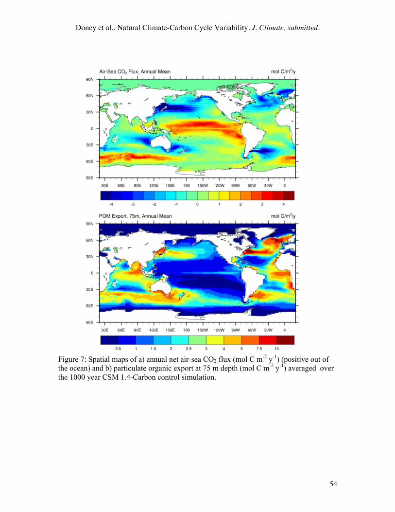
Doney et al., Natural Climate-Carbon Cycle Variability, J. Climate, submitted.
54
Figure 7: Spatial maps of a) annual net air-sea CO2 flux (mol C m-2 y-1) (positive out ofthe ocean) and b) particulate organic export at 75 m depth (mol C m-2 y-1) averaged overthe 1000 year CSM 1.4-Carbon control simulation.

Doney et al., Natural Climate-Carbon Cycle Variability, J. Climate, submitted.
55
Figure 8: Atmospheric surface CO2 fields (ppmv) from CSM 1.4-Carbon 1000 yearcontrol simulation. Panel a) shows the mean spatial distribution averaged over the bottomtwo model layers (~60 mb). Panel b) shows the mean seasonal cycle with rms interannualvariability (shading) from the model and observations at the Mauna Loa Observatory,Hawaii. The model is sampled at the nearest sigma surface to the altitude of the MaunaLoa Observatory. Observed data are from NOAA/CMDL.

Doney et al., Natural Climate-Carbon Cycle Variability, J. Climate, submitted.
56
Figure 9: Time series of global integrated, annual net a) land and b) ocean CO2 fluxes (PgC/y) from the CSM 1.4-Carbon 1000 year control simulation, highlighting the magnitudeof the interannual variability. Note the different vertical scales for the land and oceanpanels.

Doney et al., Natural Climate-Carbon Cycle Variability, J. Climate, submitted.
57
Figure 10: Spatial maps of the rms variability (1σ rms variability) of a) annual net surfaceCO2 fluxes (g C m-2 y-1) and b) annual surface atmospheric CO2 spatial concentrationanomalies (ppmv) over the 1000 year CSM 1.4-Carbon control simulation. Note the non-linear scale in panel a.

Doney et al., Natural Climate-Carbon Cycle Variability, J. Climate, submitted.
58
Figure 11: Spatial maps of the a) correlation between surface 2-m air temperature and soilmoisture for June-July-August and b) covariance of net annual ecosystem production(NEP) and annual mean non-dimensional model soil moisture stress term g(w) (Equation4) from the CSM 1.4-carbon 1000-year control run (grey regions are where thecorrelation is not significant).
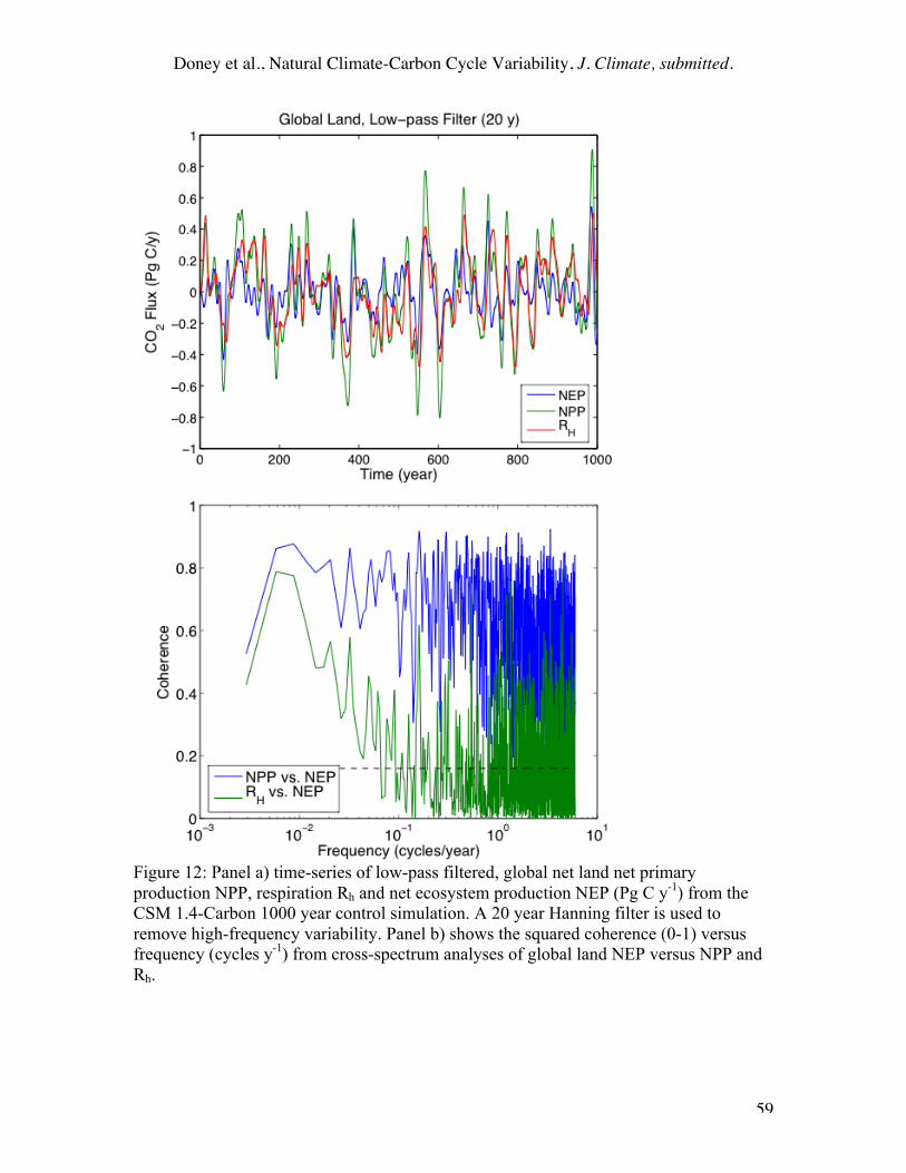
Doney et al., Natural Climate-Carbon Cycle Variability, J. Climate, submitted.
59
Figure 12: Panel a) time-series of low-pass filtered, global net land net primaryproduction NPP, respiration Rh and net ecosystem production NEP (Pg C y-1) from theCSM 1.4-Carbon 1000 year control simulation. A 20 year Hanning filter is used toremove high-frequency variability. Panel b) shows the squared coherence (0-1) versusfrequency (cycles y-1) from cross-spectrum analyses of global land NEP versus NPP andRh.

Doney et al., Natural Climate-Carbon Cycle Variability, J. Climate, submitted.
60

Doney et al., Natural Climate-Carbon Cycle Variability, J. Climate, submitted.
61
Figure 13: Spatial covariance maps of annual mean air-sea CO2 flux (positive out of theocean) and biological and physical forcing factors including a) mixed layer depth, b) seasurface temperature, c) sea surface salinity, and d) export production.

Doney et al., Natural Climate-Carbon Cycle Variability, J. Climate, submitted.
62
Figure 14: a) Power spectral density (Pg C y-1)2/(cycles y-1) versus frequency (cycles y-1)for the global integrated land and ocean CO2 fluxes from the CSM 1.4-Carbon 1000 yearcontrol simulation. The power spectra are for monthly anomalies generated by removinga mean seasonal cycle. Panel b) displays the spectrum for the total flux (land+ocean) invariance preserving form (frequency*power spectral density).

Doney et al., Natural Climate-Carbon Cycle Variability, J. Climate, submitted.
63
Figure 15: Cross-spectrum analysis for global integrated land and ocean CO2 fluxes(ΔFland vs. ΔFocean) from CSM 1.4-Carbon 1000-year control simulation. Panel a) showsthe squared coherence (0-1) versus frequency (cycles y-1). Panel b) shows the phasedifference (degrees; <0 ocean lags) between ocean and land CO2 fluxes (solid line) andocean CO2 flux and atmospheric CO2 (circles). A value of 0 degrees occurs when thetime-series are perfectly correlated and +/-180 degrees when they are perfectly anti-

Doney et al., Natural Climate-Carbon Cycle Variability, J. Climate, submitted.
64
correlated. Phase in degrees can be converted to lags/leads in years by dividing by 360(degree cycle-1) * frequency (cycles y-1). Phases are not displayed for frequencies > 0.5cycles y-1 because the ΔFland vs. ΔFocean coherences (Panel a), on average, are equivalentto zero at the 95% confidence level.
Figure 16: Time-series of low-pass filtered, global net land and ocean CO2 fluxes (Pg Cy-1) and atmospheric CO2 inventory anomaly (Pg C; scaled by dividing by 20) from theCSM 1.4-Carbon 1000 year control simulation. A 20 year Hanning filter is used toremove high-frequency variability.