Embed Size (px)
Citation preview

This document is downloaded from DR‑NTU (https://dr.ntu.edu.sg)Nanyang Technological University, Singapore.
Natural ventilation and energy efficiency of abuilding envelope in tropical climate
Wu, Xiaoying
2014
Wu, X. (2014). Natural ventilation and energy efficiency of a building envelope in tropicalclimate. Master’s thesis, Nanyang Technological University, Singapore.
https://hdl.handle.net/10356/61655
https://doi.org/10.32657/10356/61655
Downloaded on 18 Mar 2022 06:50:04 SGT
NANYANG TECHNOLOGICAL UNIVERSITY
School of Mechanical and Aerospace Engineering
Natural Ventilation and Energy
Efficiency of a Building Envelope in
Tropical Climate
WU XIAOYING
(B.Eng, Nanyang Technological University)
A Thesis Submitted to Nanyang Technological University
In Fulfillment of the Requirements for the Degree of
Master of Engineering
2013

ACKNOWLEDGEMENTS
I
ACKNOWLEDGEMENTS
I would like to express my greatest appreciation to my supervisor, Assoc. Prof. Li Hua
for his immense guidance, training and support throughout the long journey of this
project. I am also extremely grateful for the incredible amount of patience he had with me,
and for the untiring help during my difficult moments. He has imparted in me the skill of
problem solving, article writing, creative expression and perseverance which led to the
fruition of this scientific work. This project has been a most enriching experience for me
in research, thanks to Assoc. Prof. Li Hua.
I am deeply grateful to ERI@N for providing the research scholarship throughout my
Master candidature. Without the strong support of my colleagues in ERI@N, including
Prof. Subodh, Mr. Nilesh, Mr. Koh Leong Hai, Ms. Zhou Jian, Dr. Chien Szu-Cheng, this
work could not be possible. Their superb guidance, technical support and services are
essential for completion of this study. And my special thanks go to my examiners who
have taken their precious time and effort to read through and assess my thesis.
I have the great luck to work with a group of wonderful and delightful colleagues in AIT,
especially, Dr. Popovac Mirza. His guidance is really essential to me.

ACKNOWLEDGEMENTS
II
I want to thank Ms. Tong Shanshan for guiding me at the first beginning of my
simulation work. We do have spent pleasure time together to study and discuss the CFD
simulation. I thank all the people for their valuable suggestions and stimulating
discussions.
I have to say, I am very lucky to have my best friend Ms. Yan Lina with me. Without her
support and understanding, it will not be a pleasant journey for me.
Finally, I would like to show my deepest gratitude to my mother (Ren Sushuang), father
(Wu Jufang), brother (Wu Xiaobin) and my husband (Yang Bin). Without their
encouragement and understanding, this work could not be completed successfully.

ABSTRACT
III
ABSTRACT
With the development of economy, environmental issues become more critical.
Improving building energy efficiency is one of the key solutions to reduce the
environmental pollution. Building envelopes as a major component in building design
play a very essential role in building energy efficiency. In general, the building envelopes
separate the indoor and outdoor, and perform as a protection layer of living space from
the extreme harsh environment. Apart from the protection function, the building
envelopes should be aesthetic and energy efficient at the same time.
Natural ventilation is a very commonly-used traditional strategy to achieve human
comfort and energy saving simultaneously. With the development of technology,
currently various building forms can be built in reality. This gives natural ventilation
more potential in application. Therefore, the effect of building forms on natural
ventilation becomes very important for architects and developers.
In the present thesis, the academic contributions into the research area of building
performance in energy efficiency are achieved in the following two aspects.
Modeling and Simulation of Natural Ventilation for Effect of Building Forms
Regarding the structured building, it is found that common space achieves the
poorest natural ventilation over a year, excluding rooftop. This is attributable to
the low porosity of building.
Regarding the porous building, it is concluded that, with the increase of the
percentage of void inside the building, common spaces results in higher wind

ABSTRACT
IV
speed, and the percentage of thermal comfortable area also increases, contrary to
structured building.
Regarding the free-form architecture building, it is observed that the wind
velocity profile inside the atrium is highly correlated to the floor level. This is
attributed to the stack effect. In addition, the internal airflow speed is almost
independent of the external wind.
Modeling and Simulation of Energy Efficiency for Effect of Building Envelope
In terms of external building envelope, a reduction in cooling load is achieved by
increasing either the vertical length L, or by reducing the horizontal distance D
between building envelope and wall.
It is shown that a maximum energy efficiency of 13% is achieved by increasing
length L to 50% of the building height H.
In general, the external envelope tends to make a more significant contribution to
improvement of energy efficiency for buildings with windows, compared with
windowless building.

TABLE OF CONTENTS
V
TABLE OF CONTENTS
ACKNOWLEDGEMENTS ............................................................................. I
ABSTRACT ............................................................................................. III
TABLE OF CONTENTS ............................................................................... V
LIST OF FIGURES ...................................................................................... IX
LIST OF TABLES ....................................................................................... XV
CHAPTER 1 INTRODUCTION ................................................................. 1
1.1 Background ............................................................................................................. 1
1.2 Tropical Climate of Singapore ................................................................................ 4
1.3 Natural Ventilation.................................................................................................. 7
1.3.1 Definition of Natural Ventilation .................................................................... 7
1.3.2 Classification of Natural Ventilation ............................................................... 8
1.4 Building Envelope ................................................................................................ 11
1.4.1 Definition of Building Envelope ................................................................... 11
1.4.2 Classification of Building Envelope Design ................................................. 13
1.5 Motivation and Objectives .................................................................................... 16
1.6 Organization of Report ......................................................................................... 20
CHAPTER 2 LITERATURE REVIEW .................................................... 22
2.1 Energy Efficiency of Building Envelope .............................................................. 22
2.1.1 Envelope Thermal Transfer Value (ETTV) .................................................. 22
2.1.2 Correlation between Building Design and Energy Efficiency ...................... 24
2.1.3 Overhang Shading Devices ........................................................................... 26

TABLE OF CONTENTS
VI
2.1.4 Louvers Shading Devices .............................................................................. 28
2.1.5 Double Skin ................................................................................................... 29
2.2 Effect of various Building Envelope on Natural Ventilation................................ 31
2.2.1 Louvers Shading Devices .............................................................................. 31
2.2.2 Double Skin ................................................................................................... 32
2.3 Thermal Comfort Analysis Models for Naturally Ventilated Spaces ................... 34
CHAPTER 3 NATURAL VENTILATION FOR EFFECT OF BUILDING
FORMS ............................................................................... 37
3.1 Methodology for Simulation of Natural Ventilation ............................................ 37
3.1.1 Laminar Flow or Turbulence Flow ............................................................... 38
3.1.2 Turbulence Flow Model ................................................................................ 39
3.1.3 Computational Domain ................................................................................. 40
3.1.4 Boundary Conditions ..................................................................................... 41
3.1.5 Post Processing .............................................................................................. 41
3.2 Project I: A Structured Research Building CleanTech Two ................................ 42
3.2.1 Description of Model ..................................................................................... 44
3.2.2 Boundary Condition ...................................................................................... 45
3.2.3 Results and Discussion .................................................................................. 46
3.2.4 Summary ....................................................................................................... 51
3.3 Project II: A Porous Academic Building North Spine Academic Building.......... 53
3.3.1 Description of Model ..................................................................................... 54
3.3.2 Boundary Conditions ..................................................................................... 55
3.3.3 Results and Discussion .................................................................................. 56
3.3.4 Summary ....................................................................................................... 62

TABLE OF CONTENTS
VII
3.4 Project III: A Free-Form Academic Building Learning Hub................................ 62
3.4.1 Description of Model ..................................................................................... 64
3.4.2 Boundary Conditions ..................................................................................... 67
3.4.3 Results and Discussion .................................................................................. 68
3.4.4 Summary ....................................................................................................... 73
CHAPTER 4 ENERGY EFFICIENCY FOR EFFECT OF BUILDING
ENVELOPE ........................................................................ 75
4.1 Methodology for Simulation of Building Energy ................................................. 75
4.1.1 Geometries of Simulation Models ................................................................. 76
4.1.2 Assumption and input of Simulation Model ................................................. 82
4.1.3 Post Process ................................................................................................... 89
4.2 Effect of Plane-Plate Envelope ............................................................................. 90
4.2.1 Effect of Distance between Building Envelope and Wall on the relationship
of Energy Efficiency and Length of Building Envelope ............................... 90
4.2.2 Effect of Length of Building Envelope on the relationship of Energy
Efficiency and Distance between Building Envelope and Wall. ................... 94
4.2.3 Effect of Angle θ between Building Envelope and Wall on Energy Efficiency
....................................................................................................................... 97
4.2.4 Effect of Location of Window on Energy Efficiency ................................. 103
4.2.5 Remarks ....................................................................................................... 106
4.3 Effect of Curved-Shell Envelope ........................................................................ 107
4.3.1 Effect of Distance between Building Envelope and Wall on the relationship
of Energy Efficiency and Length of Building Envelope ............................. 107

TABLE OF CONTENTS
VIII
4.3.2 Effect of Length of Building Envelope on the relationship of Energy
Efficiency and Distance between Building Envelope and Wall .................. 110
4.3.3 Remarks ....................................................................................................... 112
4.4 Effect of Vertical Green Envelope ...................................................................... 113
4.4.1 Effect of Mesh Size on Energy Efficiency .................................................. 113
4.4.2 Effect of Porosity Ratio on Energy Efficiency ............................................ 114
4.4.3 Remarks ....................................................................................................... 117
4.5 Effect of Internal Smart Blinds ........................................................................... 117
4.5.1 Effect of Smart Blinds on indoor ambient temperature .............................. 117
4.5.2 Effect of Smart Blinds on wall temperature of east façade ......................... 119
4.5.3 Remarks ....................................................................................................... 122
CHAPTER 5 CONCLUSION AND FUTURE WORK .......................... 124
5.1 Conclusion .......................................................................................................... 124
5.2 Future work ......................................................................................................... 127
PUBLICATIONS ARISING FROM THE THESIS .................................. 129
REFERENCES ........................................................................................... 130

LIST OF FIGURES
IX
LIST OF FIGURES
Figure 1.1 Rising trend of global energy consumption in different countries. [3] ............. 2
Figure 1.2 Typical breakdown of energy consumption within a commercial building with
the biggest use of electricity by air-conditioning and mechanical-ventilation
(ACMV). ................................................................................................................. 3
Figure 1.3 Sun-path diagram in Singapore, in which the sun traverses directly above the
equator in September and off the equator in June and December [7]. .................... 5
Figure 1.4 Direction of prevailing wind in Singapore. ....................................................... 6
Figure 1.5 Cross ventilation through a building. ................................................................ 9
Figure 1.6 Stack ventilation within a building. ................................................................. 10
Figure 1.7 Building envelope with exterior and interior environment [11]. ..................... 12
Figure 1.8 Self-shaded envelope of Concourse in Singapore. .......................................... 14
Figure 1.9 An example of exterior louvers shading design [12]....................................... 14
Figure 1.10 Overhang design in eave condition [13]. ....................................................... 15
Figure 1.11 Double skin envelope [12]............................................................................. 16
Figure 1.12 External building envelope adopted in this thesis. ........................................ 18
Figure 1.13 Basic case adopted in this thesis. ................................................................... 19
Figure 1.14 Special cases resulted from the general case. ................................................ 20
Figure 2.1 Relative ranking of influencing parameters on ETTV when WWR varies [15].
............................................................................................................................... 25
Figure 2.2 Energy saving efficiency from exterior shading observed from variation in AC
electricity usage density in office buildings. ......................................................... 26
Figure 2.3 Four different configurations of shading devices [22]. ................................... 29

LIST OF FIGURES
X
Figure 2.4 Impact of different insulation on energy savings of a double-skin in a north-
south building [24]. ............................................................................................... 30
Figure 2.5 Velocity vectors on a longitudinal-section (a) wind-tunnel experiment
(CEDVAL), (b) CFD simulations [34]. ................................................................ 34
Figure 3.1 Impression drawing of CTT building. (Source: JCPL). .................................. 42
Figure 3.2 Computational domain of CFD simulation for CTT project including existing
and future buildings in CleanTech Park within next 20 years. ............................. 43
Figure 3.3 CTT building model in CFD simulation by gambit software.......................... 43
Figure 3.4 Diagram of CTT model setup for ventilation simulation. ............................... 44
Figure 3.5 Velocity vectors in north wind scenario. ......................................................... 47
Figure 3.6 Velocity vectors in northeast wind scenario. ................................................... 48
Figure 3.7 Velocity vectors in south wind scenario. ......................................................... 49
Figure 3.8 Site plan of Clean Tech Park. .......................................................................... 49
Figure 3.9 Velocity vectors in southeast wind scenario. .................................................. 50
Figure 3.10 Average wind velocity in a year. ................................................................... 52
Figure 3.11 Impression drawing of NSAB building (Source: ADDP). ............................ 53
Figure 3.12 Computational domain of the NSAB model ................................................. 54
Figure 3.13 Top view of NSAB and neighbor buildings in CFD simulation model. ....... 54
Figure 3.14 Plane view of velocity contour of seven levels within NSAB under north
wind scenario. ....................................................................................................... 58
Figure 3.15 Cross section view: (a) cross section line; (b) velocity vector within the small
atrium area; (c) velocity contour. .......................................................................... 58
Figure 3.16 Plane view of velocity contour of seven levels within NSAB in northeast
wind scenario. ....................................................................................................... 59

LIST OF FIGURES
XI
Figure 3.17 Cross section view: (a) cross section line; (b) velocity vector within the small
atrium area; (c) velocity contour. .......................................................................... 59
Figure 3.18 Plane view of velocity contour of seven levels within NSAB in south wind
scenario. ................................................................................................................ 60
Figure 3.19 Cross section view: (a) cross section line; (b) velocity vector within the small
atrium area; (c) velocity contour. .......................................................................... 60
Figure 3.20 Plane view of velocity contour of seven levels within NSAB in southeast
wind scenario. ....................................................................................................... 61
Figure 3.21 Cross section view: (a) cross section line; (b) velocity vector within the small
atrium area; (c) velocity contour. .......................................................................... 61
Figure 3.22 Impression drawing of LH building. (Source: NTU) .................................... 63
Figure 3.23 Computational domain for LH model ........................................................... 65
Figure 3.24 Cross section view of LH model. .................................................................. 65
Figure 3.25 Top view of LH model in CFD simulation. .................................................. 66
Figure 3.26 Cross section view (Level 5) of LH building model in which gaps and
staircases together with four selected measured points are shown. ...................... 66
Figure 3.27 Velocity vectors of 9 floors for north wind scenario. .................................... 69
Figure 3.28 Circulation winds in between the buildings. ................................................. 70
Figure 3.29 Velocity vectors of 9 floors for northeast wind scenario. ............................. 71
Figure 3.30 Velocity vectors of 9 floors for south wind scenario. ................................... 72
Figure 3.31 Velocity vectors of 9 floors for southeast wind scenario. ............................. 73
Figure 4.1 Geometry of the basic energy simulation model without window. ................. 76
Figure 4.2 Geometry of basic energy simulation model with window on east wall. ........ 77
Figure 4.3 Geometric parameters of plane-plate envelope. .............................................. 77

LIST OF FIGURES
XII
Figure 4.4 Geometric parameters of curved-shell envelope for the effect on building
energy efficiency in the vertical envelope design (a) and the horizontal overhang
design (b). ............................................................................................................. 78
Figure 4.5 Geometry of simulation models with vertical green envelope with 50%
porosity ratio for building with window (a) and windowless building (b). .......... 80
Figure 4.6 Geometry of simulation models with vertical green envelope which has
porosity ratio of 10% (a), 20% (b), 30% (c), 40% (d), 50% (e), 60% (f), 70% (g),
80% (h) and 90% (i). ............................................................................................. 80
Figure 4.7 Geometry of simulation model with internal smart blind. .............................. 81
Figure 4.8 Schedule of lighting system on weekdays. ...................................................... 84
Figure 4.9 Schedule of lighting system on Saturday. ....................................................... 84
Figure 4.10 Schedule of occupancy on weekdays. ........................................................... 85
Figure 4.11 Schedule of occupancy on Saturday. ............................................................. 85
Figure 4.12 Schedule of equipment on weekdays. ........................................................... 86
Figure 4.13 Schedule of equipment on Saturday. ............................................................. 86
Figure 4.14 Effect of distance (D) between building envelope and wall on the relationship
of energy efficiency and length (L) of external plane-plate building envelope for
building with window. .......................................................................................... 91
Figure 4.15 Effect of distance (D) between building envelope and wall on the relationship
of energy efficiency and length (L) of external plane-plate building envelope for
building without window. ..................................................................................... 93
Figure 4.16 Effect of length (L) of building envelope on the relationship between building
cooling load and distance (D) between plane-plate envelope and wall for building
with window.......................................................................................................... 94

LIST OF FIGURES
XIII
Figure 4.17 Effect of length (L) of building envelope on the relationship between building
cooling load and distance (D) between plane-plate envelope and wall for building
without window. ................................................................................................... 96
Figure 4.18 Effect of the angle θ between plane-plate envelope and wall on building
cooling load for the building with window at 025.0/ HD . .............................. 98
Figure 4.19 Effect of angle θ between plane-plate envelope and wall on building cooling
load for building with window at 125.0/ HD . .................................................. 99
Figure 4.20 Effect of angle θ between plane-plate envelope and wall on building cooling
load for building with window at 25.0/ HD . .................................................... 99
Figure 4.21 Effect of angle θ between plane-plate envelope and wall on building cooling
load for building with window at 5.0/ HD . .................................................... 100
Figure 4.22 Effect of angle θ between plane-plate envelope and wall on building cooling
load for building with window at 75.0/ HD . .................................................. 100
Figure 4.23 Effect of angle θ between plane-plate envelope and wall on building cooling
load for building with window at 1/ HD . ....................................................... 101
Figure 4.24 Effect of angle θ between plane-plate envelope and wall on building cooling
load for windowless building. ............................................................................. 103
Figure 4.25 Bar chart of indoor cooling load with or without window and with envelope
on east or west. .................................................................................................... 105
Figure 4.26 Effect of distance between Building Envelope and Wall (D) on the
relationship of energy efficiency and length of external plane-plate building
envelope (L) for building with window and vertical curved-shell envelope. ..... 107

LIST OF FIGURES
XIV
Figure 4.27 Effect of distance between Building Envelope and Wall (D) on the
relationship of energy efficiency and length of external plane-plate building
envelope (L) for building with window and horizontal curved-shell envelope. . 108
Figure 4.28 Effect of length of building envelope (L) on the relationship between building
cooling load and distance between plane-plate envelope and wall (D) for building
with window and vertical curved-shell envelope. ............................................... 110
Figure 4.29 Effect of distance between building envelope and wall (D) on building
cooling load for building with window and horizontal curved-shell envelope. . 111
Figure 4.30 Three simulation models of vertical green envelope with 50% porosity and
different mesh size of 1m (a), 0.5m (b), and 0.25m (c). ..................................... 114
Figure 4.31 Effect of porosity ratio of building envelope on cooling load for building
with window........................................................................................................ 115
Figure 4.32 Effect of porosity ratio of building envelope on cooling load for building
with window........................................................................................................ 116
Figure 4.33 External solar radiation and indoor ambient temperature at the center point
inside the building with smart blind (solid blue), no blind (solid red) and static
blind (solid green) on 21st June. .......................................................................... 119
Figure 4.34 External solar radiation and indoor ambient temperature on east façade of the
building with smart blind (solid blue), no blind (solid red) and static blind (solid
green) on 21st June. ............................................................................................. 121

LIST OF TABLES
XV
LIST OF TABLES
Table 1.1 Typical Energy Consumption in Major Countries for Office Buildings [5-6]. .. 3
Table 1.2 Mean wind speed and frequency of prevailing winds in Singapore. .................. 7
Table 1.3 Monthly statistics of wind directions in Singapore. ........................................... 7
Table 2.1 Impact of different design factors on annual cooling load. .............................. 24
Table 2.2 Energy saving efficiency from exterior shading observed from variation in AC
electricity usage density in office buildings. ......................................................... 27
Table 3.1 Boundary conditions for CTT model. ............................................................... 45
Table 3.2 Average wind speed for all the public areas in CTT. ....................................... 51
Table 3.3 Boundary conditions for CFD simulation of NSAB. ........................................ 56
Table 3.4 Area-weighted average wind speed and percentage of thermal comfort inside
the common spaces in seven levels for four wind scenarios. ............................... 62
Table 3.5 Boundary conditions for Learning Hub natural ventilation simulation. ........... 67
Table 3.6 Percentage of comfort areas. ............................................................................. 74
Table 4.1 Blind tilt angle and openness factor calculated based on vector of solar incident
ray. ........................................................................................................................ 82
Table 4.2 Cooling load contribution for energy simulation .............................................. 83
Table 4.3 Solar radiation intensity and outdoor temperature in Singapore on 21st June [51].
............................................................................................................................... 88
Table 4.4 Boundary conditions in CFD simulation. ........................................................ 88
Table 4.5 Material properties used in CFD simulation [12]. ........................................... 89
Table 4.6 Minimum cooling load by varying D/H for building with window and plane-
plate envelope. ...................................................................................................... 92

LIST OF TABLES
XVI
Table 4.7 Minimum cooling load with varying L/H for building with window and plane-
plate envelope. ...................................................................................................... 95
Table 4.8 Comparison study of minimum cooling load with θ. ..................................... 102
Table 4.9 Minimum cooling load with varying L/H for building with window and vertical
curved-shell envelope. ........................................................................................ 108
Table 4.10 Minimum cooling load with varying L/H for building with window and
horizontal curved-shell envelope. ....................................................................... 109
Table 4.11 Minimum cooling load with varying D/H for building with window and
vertical curved-shell envelope. ........................................................................... 111
Table 4.12 Ambient temperature at the center point inside the building with smart blind
or static blind or without blind. ........................................................................... 118
Table 4.13 Average surface temperature on building east façade with smart blind or static
blind or without blind.......................................................................................... 120

CHAPTER 1 INTRODUCTION
1
CHAPTER 1 INTRODUCTION
In this chapter, the importance of building energy performance in recent years is
overviewed, followed by the global trend of building energy consumption in different
countries. The definition and classification of natural ventilation and building envelope
are then introduced correspondingly. Finally, the motivation of this study and
organization of this report are outlined.
1.1 Background
With the development of economic, global energy consumption rises as shown in Figure
1.1 , and the environmental issue becomes more and more critical. All the items, such as
air pollution, water pollution, land pollution, climate change and global warming, appear
in daily life more and more frequently. Generally, most of the environmental crises
originate from energy related problems. Without solving the energy issues, there will be
no sustainable development.
The building and construction industry is a highly-contaminative, high energy-consuming
and high carbon-emissive industry. For example, in United States, 41% of primary
energy is consumed by building sectors [1], and in Singapore, buildings consume about
31% of total electricity, and after adding households’ consumption the number jumps to
49% of all electricity [2]. The trend of energy consumption in buildings [3] is shown in
Figure 1.1, in which, electricity, natural gas and petroleum are the total building
expenditures. Energy use in buildings was increased by 61.3%, compared with year 1980.
Thus, the building energy efficiency becomes critical nowadays.

CHAPTER 1 INTRODUCTION
2
Within the typical lifespan of a building, there are two phases: construction and operation.
In the construction phase, major energy consumption comes from building materials,
transportation and construction. For example, cement is a very common building material.
In China, 1 ton of CO2, 0.74 kg of SO2 and 130 kg of dust are generated, in order to
produce one ton of cement. The production of raw materials, such as steel, cement, flat
glass, ceramic, brick and aggregates, consumes over 1.6 × 10⁸ ton of coal per year, about
13% of China’s total energy output [4]. In the operation phase, the main energy use is by
electricity, which is used for air-conditioning system, lighting system, vertical
transportation system, ventilation system, equipment and other miscellaneous, in order to
maintain indoor comfort and human life.
Figure 1.1 Rising trend of global energy consumption in different countries. [3]

CHAPTER 1 INTRODUCTION
3
Figure 1.2 Typical breakdown of energy consumption within a commercial building
with the biggest use of electricity by air-conditioning and mechanical-ventilation
(ACMV).
Table 1.1 Typical Energy Consumption in Major Countries for Office Buildings [5-6].
Energy end-uses USA (%) UK (%) Spain (%) Singapore (%)
HVAC 48 55 52 52
Lighting 22 17 33 12
Equipment (appliances) 13 5 10 25
DHW (domestic hot water) 4 10 – -
Food preparation 1 5 – -
Refrigeration 3 5 – -
Others 10 4 5 11
The percentage distribution of energy consumption inside an office building is shown in
Figure 1.2 [5]. The office building energy consumptions in four countries is compared as
shown in Table 1.1. There are three key energy end uses inside an office building, namely
Highest
Consumption

CHAPTER 1 INTRODUCTION
4
heating, ventilation and air-conditioning (HVAC) systems, lighting systems and
equipment. These end-uses total to about 86% of the total energy consumption. However,
the energy consumption by equipment is very user dependent and developers could
control this part during the building design. Thus, the two controllable big energy
consumers are HVAC and lighting system. HVAC takes around 50% of the total energy
consumption, and lighting around 20% of the total energy consumption. Hence, in order
to improve building performance, HVAC and lighting systems are the focus parts to
reduce energy consumption.
1.2 Tropical Climate of Singapore
Understanding the climate around the building is also very important since the
performance of the building is climate dependent. In this report, buildings in Singapore
are chosen to be studied.
Singapore lies within the tropical climatic belt, with geographical coordinates 1.37 of
north latitude and 103.75 of east longitude. Its tropical climate is characterized by
uniform temperature and pressure, high humidity and abundant rainfall. There are no
distinct wet or dry seasons. Normally the maximum rainfall occurs in December and
April, and the drier months are usually in February and July. The temperature differences
in Singapore are not distinct, with the minimum diurnal temperature ranging from 23oC
to 26oC and the maximum diurnal temperature from 31
oC to 34
oC. Similarly, there is no
significant variation in pressure. The diurnal relative humidity ranges in the high 90% in
the early morning to around 60% in the mid-afternoon. The mean relative humidity value
is 84% and it often reaches 100% during prolonged heavy rain.

CHAPTER 1 INTRODUCTION
5
Besides the factors mentioned above, solar-energy, the major heat gain in natural and
artificial ventilated buildings in the tropics, is another important components of the
climate. In Singapore, the sun traverses east-west directly above our buildings most of the
time, which is shown in Figure 1.3. In summer, the sun is in the north of Singapore, while
in winter, the sun is in the south. In this report, 21st June is used to represent the summer
time and similarly 21st
December is used to represent the winter time. Normally the north
and south sides of the building are only exposed to the sun during half of the year, and
the east and west sides of the building are exposed to the sun everyday within a year.
Figure 1.3 Sun-path diagram in Singapore, in which the sun traverses directly above
the equator in September and off the equator in June and December [7].

CHAPTER 1 INTRODUCTION
6
Figure 1.4 Direction of prevailing wind in Singapore.
The wind situation is also very important in building energy efficiency, especially for
naturally ventilated buildings. In Singapore, there are two main monsoon seasons: north
monsoon (from December to early March) and south monsoon (from June to September).
Both seasons are separated by two relatively short inter-monsoon periods (late March to
May and October to November). The map of Singapore with indicated directions for
north and south monsoons was shown in Figure 1.4. During the north monsoon period,
the northeast or north winds prevail, with wind speed reaching up to 11 m/s in the months
of January and February. Southeast or south winds prevail during the south monsoon
period with wind speed reaching up to 6 m/s. The sky is mostly cloudy, with frequent
afternoon showers during these times. Light and variable winds occur during the two
inter-monsoon periods. The mean wind speed for the prevailing winds in Singapore is
shown in Table 1.2 [8]. The monthly statistics of wind direction is shown in Table 1.3 [9].

CHAPTER 1 INTRODUCTION
7
Table 1.2 Mean wind speed and frequency of prevailing winds in Singapore.
Wind Direction Mean Speed (m/s) Frequency
North 2 22.2%
Northeast 2.9 22.2%
South 2.8 27.8%
Southeast 3.2 27.8%
Table 1.3 Monthly statistics of wind directions in Singapore.
Month Wind Direction
Jan N/NE
Feb N/NE
Mar N/NE
Apr variable
May S/SE
Jun S/SE
Jul S/SE
Aug S/SE
Sep S/SE
Oct variable
Nov variable
Dec N/NE
1.3 Natural Ventilation
1.3.1 Definition of Natural Ventilation
Natural ventilation is the process of supplying and removing air through an indoor space
without using mechanical systems. Natural ventilation is important in removing heat,
water vapor and CO2 released by human body, and hence controls indoor thermal comfort.

CHAPTER 1 INTRODUCTION
8
In relation to the criterion of good energy efficient design and indoor thermal comfort,
natural ventilation becomes a very attractive solution to ensure both good indoor air
quality and acceptable comfort conditions in many regions. Natural ventilation seems to
provide an answer to many complaints about the usage of mechanical ventilation systems,
and it can provide a more energy efficient, healthier and more comfortable environment if
integrated properly.
However ‘natural’ also means that behavior is random and efficient control of the
building is difficult. Furthermore, in many urban environments outdoor air conditions and
acoustics may not be acceptable because of air and noise pollution. Natural ventilation in
this kind of situation need special design features in order to avoid a direct link between
indoor and outdoor environments. In order to be effective, natural ventilation also
requires a high degree of permeability within the building. In the case of deep plan design,
in which the horizontal distance from one side external wall to the other side
external wall is many times greater than the floor to floor height, fresh air delivery or a
good mixture of air may not be possible without special design considerations. Physical
features such as neighboring building walls, trees and others, which may influence air
movement, must be taken into account in natural ventilation design.
1.3.2 Classification of Natural Ventilation
There are two types of natural ventilation in buildings: wind driven ventilation and
buoyancy driven ventilation. Wind driven ventilation, or cross ventilation, is formed by
pressure difference between inlet and outlet. The inlet is the opening where the wind can
blow through and enter the indoor environment, and the outlet is the opening where the

CHAPTER 1 INTRODUCTION
9
wind can blow through and leave the indoor space. Sometimes the inlet and outlet could
be the same opening depending on the building design. Cross ventilation could be further
classified into single-sided ventilation and double-sided ventilation. Buoyancy driven
ventilation is formed by temperature difference between inlet and outlet. It could be
further classified into stack effect, night cooling and thermal mass based on temperature
difference mechanisms.
1.3.2.1. Wind Driven Ventilation
The concept of cross ventilation is simple and has to do with pressure difference between
the outdoor and indoor environment. When wind hits one side of a building (the
windward side), the air speeds up in order to flow around the building to the opposite side
of the building (the leeward side).This creates a positive pressure on the windward side
and a negative pressure on the leeward side. If windows in a building are open, air is
forced to enter from the windward side and leave at the leeward side, which creates a
force for air crossing through the building, as shown in Figure 1.5. In order to produce
the maximum total airflow through a space, both inlet and outlet openings should be as
large as possible, and the inlet opening should be much smaller than the outlet one.
Figure 1.5 Cross ventilation through a building.

CHAPTER 1 INTRODUCTION
10
1.3.2.2. Buoyancy Driven Ventilation
The concept of the stack effect has to do with temperature differentiation between the
indoor and outdoor environment as shown in Figure 1.6. Hot air rises within a building
and escapes through an opening on the roof and pulls cooler air from outside into the
building. This creates a cross airflow within the interior space and creates ventilation for
the building. A stack increases this effect, and the longer the stack the greater the airflow
obtained. Stack ventilation works regardless of whether there is any prevailing wind
available. Even though the movement of air is at a relatively slow speed, the results from
the stack effect may be adequate to supply fresh air and produce convection cooling.
However, these forces are rarely sufficient to create the required air movement for
thermal comfort in certain hot zones of a living space. The only natural force can be
relied on for this purpose is the dynamic effect of wind, and great effort must be made to
capture this force.
Figure 1.6 Stack ventilation within a building.
The concept of night cooling rests on the fact that outdoor temperatures are usually lower
at night than during the day. Cooler night air is brought into the interior space to flush out
warm stale air that has accumulated during the day. The night cooling concept is
relatively simple to be implemented, but the security risks should be considered. If the

CHAPTER 1 INTRODUCTION
11
windows are left open during the night, over-cooling may occur and then condensation
issues on the inner face of windows occur when air-conditioning is used on the next day.
Thermal mass is incorporated into a building structure to absorb heat during the daytime
hours, in order to keep the interior space cool. Cooler outside air can be brought in to
bring the temperature of the thermal mass back down to preoccupancy levels at night.
Typically, this mass is incorporated into ceiling spaces and walls in the form of masonry
construction. This is an effective method of providing ventilation to buildings. However,
the use of thermal mass is the most challenging in hot and humid climate, where night
temperatures remain elevated. It should be strategically located to prevent overheating in
such climate.
1.4 Building Envelope
1.4.1 Definition of Building Envelope
Building envelope, also known as building enclosure, is one of the fundamental
components in a building. It separates unconditioned exterior environment from
conditioned interior space, as illustrated in Figure 1.7. Building envelope furnishes
appearance of buildings and also functions as load bearing, active or passive
environmental control and creative expression for architect [10]. The envelope is made
up of all the exterior components of the building, including walls, roof, foundations,
windows, and doors.

CHAPTER 1 INTRODUCTION
12
Figure 1.7 Building envelope with exterior and interior environment [11].
Generally the functions of the building envelope can be categorized into 3 groups:
structural support, control and finish. The structural maintains all the mechanical loadings
imposed on the building. The control function is to govern flow of mass and energy such
as moisture, air, heat and sound in between interior and exterior environments. The finish
function is to end the enclosure surfaces and the interfaces of the envelope, meaning that
the façade design and interfaces of wall are all considered as the finish function of
envelope.
Building envelope, working as the middle layer between the indoor and outdoor, plays a
very important role in mass and energy transfer, especially in Singapore whose climate is
hot and humid. Human tends to use air-conditioning system to achieve indoor thermal
comfort. Due to the temperature difference between the indoor and outdoor, there is heat
conduction through the walls, roofs, floors and windows. There is also solar radiation
through the glass windows and heat loss due to air infiltration. All these activities

CHAPTER 1 INTRODUCTION
13
increase the internal cooling load, and results in an increase in the energy consumption
and cost. In order to achieve better building energy efficiency, there is a need to regulate
the design of building envelopes to minimize heat gains into the interior spaces and
energy lost.
1.4.2 Classification of Building Envelope Design
Based on the number of layers, building envelopes are classified into single skin envelope
and double skin envelope. For the single skin envelope, based on shading strategies, it is
further classified into self-shading building envelope and with-shading devices building
envelope.
1.4.2.1. Single-Skin Envelope
For single-skin envelope, there are two common shading strategies: self-shading and
extra shading devices. The self-shaded design is shown in Figure 1.8, and the louvers and
the overhang shading device design are shown in Figure 1.9 and Figure 1.10 separately.
Generally architectures prefer to use overhangs in building because it also gives the
building character. The main function of overhang is to protect the windows or walls
from outdoor climate and performs like shading device and rain shelter.

CHAPTER 1 INTRODUCTION
14
Figure 1.8 Self-shaded envelope of Concourse in Singapore.
Figure 1.9 An example of exterior louvers shading design [12].

CHAPTER 1 INTRODUCTION
15
Figure 1.10 Overhang design in eave condition [13].
1.4.2.2. Double-Skin Envelope
The double skin façade or double skin envelope illustrated in Figure 1.11 is a system of
building consisting of two skins placed in such a way that air flows in the intermediate
cavity. The ventilation of the cavity can be natural, fan supported or mechanical. Apart
from the type of the ventilation inside the cavity, the origin and destination of the air can
differ depending mostly on climatic conditions, the use, the location, the occupational
hours of the building and the HVAC strategy. Double skin façade could be classified into
multi-storey façade, shaft box façade, corridor façade and box window façade, based on
different geometries of building façade [12]. In addition, based on the natural of
ventilation inside the cavity between the first and second skins, double skin façade could
also be categorized as active double skin façade and passive double skin façade. If the
ventilation inside the cavity is driven by mechanical method, such as fans, it is named as

CHAPTER 1 INTRODUCTION
16
active double skin. Otherwise, it is named as passive double skin, meaning that there is
no power consumed to introduce the ventilation inside the cavity.
Figure 1.11 Double skin envelope [12]
1.5 Motivation and Objectives
Singapore is a tropical country with hot and humid climate. Here air-conditioning system
plays an essential role in people’s daily work and life. Therefore, the energy efficiency of
building envelope becomes essential, and natural ventilation as a method to reduce the
dependency on air conditioning system becomes very important as well. So in this thesis,
the effect of building forms on the natural ventilation and the effect of parameters of
building envelope on the building energy efficiency are studied through mathematical
modeling and simulation.
For the effect of building forms on the natural ventilation, three real buildings are studied
by modeling and simulation to find out how the building form affects the natural

CHAPTER 1 INTRODUCTION
17
ventilation in real building projects. The first one is CleanTech Two (CTT) building
which has structured architecture design. The second one is North Spine Academic
Building (NSAB) which has porous architecture design, located inside NTU. Finally, the
third one is Learning Hub (LH) building which has free-form architecture design located
inside NTU. There are two main reasons for choosing these three buildings. One is that
all these three buildings are targeted to get Green Mark Platinum award which require at
least 30% of energy saving and even NSAB is targeted to get Green Mark PlatinumPlus
which require more than 40% energy saving. Such big energy saving requirement results
that the building should be designed in a passive way to avoid the energy consumption by
air-conditioning which is a big energy consumer. The other is that the building time of
three buildings is very near (CTT was planned in 2011 and is under construction now,
NSAB is in the planning stage now and will be under construction in 2015 and LH was
planned in 2012 and is also under construction now), and such near time means that the
available technologies, materials, construction work are almost the same. In one sentence,
these three buildings have the similar target and same available resources.
For the effect of parameters of building envelope on the energy efficiency, although
many researchers have done relevant studies in this area with the focus on a very specific
design, such as overhang, double skin façade, louvers and self-shading, there is no
general guideline for design of building shading devices outside the building envelope, in
terms of building energy efficiency. Therefore, this research aims to develop a general
guideline for building envelopes in terms of energy efficiency through a holistic
investigation of all key parameters involved in a shading device.

CHAPTER 1 INTRODUCTION
18
The model used in this study is shown in Figure 1.12, in which a single-storey building
with 10×10×4 m3 is assumed, and the red lines represent a general building envelope
outside the building wall. The basic case is shown in Figure 1.13, in which there is only
building wall without any shading devices or double skin.
Figure 1.12 External building envelope adopted in this thesis.

CHAPTER 1 INTRODUCTION
19
Figure 1.13 Basic case adopted in this thesis.
This general building envelope includes the double skin design and overhang design,
which can be illustrated in Figure 1.14.
Horizontal overhang design is resulted when the θ = 90°.
General overhang design is resulted when D = 0 and θ ≠ 90°.
Double skin design is resulted when θ = 0° and D ≠ 0. The only difference
between the two cases at the bottom is the 1st part of the building envelope. One
has the 1st part and the other has not.
The objective of this study is to develop a guideline for design of a building envelope
with highly efficient energy through parametric studies. As indicated in the Figure 1.12,
the parameters are:
D: the length of the 1st part of building envelope.
L: the length of the 2nd
part of building envelope.

CHAPTER 1 INTRODUCTION
20
Porosity of building envelope.
Fenestration location on the wall.
The angle θ between building envelope and wall.
Figure 1.14 Special cases resulted from the general case.
1.6 Organization of Report
Chapter 1 presents the background information related to this study, motivation and
objectives of this study.
Chapter 2 provides a review of building energy efficiency studies and natural ventilation
studies of three type of shading devices: overhang, louvers and double skin. The indoor

CHAPTER 1 INTRODUCTION
21
comfort standard and regulations on building envelope energy performance are also
included. Building design factors on building energy efficiency are covered as well.
Chapter 3 investigates the effect of building forms on the natural ventilation via
computational fluid dynamic (CFD) simulation.
Chapter 4 investigates the effect of external envelope on building energy efficiency via
energy simulation using EnergyPlus and Open Studio, and the effect of internal shading
device on building energy efficiency via CFD simulation.
Chapter 5 concludes all the findings and details the recommendation the future work.

CHAPTER 2 LITERATURE REVIEW
22
CHAPTER 2 LITERATURE REVIEW
This chapter reviews the energy efficiency with various building design factors, followed
by the standard of indoor thermal comfort. The regulations on building envelope energy
efficiency are then discussed. Previously published research work on the energy
efficiency of three kinds of building shading devices, overhang, louvers and double skin
is reviewed. Finally, research work on natural ventilation of louvers and double skin is
also reviewed.
2.1 Energy Efficiency of Building Envelope
2.1.1 Envelope Thermal Transfer Value (ETTV)
An envelope thermal performance standard known as Overall Thermal Transfer Value
(OTTV) was published by Building Control Regulations in 1979, in order to regulate
building envelopes designs and control solar heat gains by buildings. However, the
standard is only applicable to air conditioned non-residential buildings. In early 2000, a
major review on OTTV was conducted to work out a more accurate calculation that was
named Envelope Thermal Transfer Value (ETTV) [14]. ETTV was still only applicable
to non-residential buildings that are air-conditioned during day time.
In 2008 the ETTV is extended to cover the residential buildings [15], in which the air-
conditioners are usually turned on during the daytime. In order to differentiate roof from
ETTV, Residential Envelope Transmittance Value (RETV) was proposed, in which the
air-conditioners are usually turned on during evening.

CHAPTER 2 LITERATURE REVIEW
23
In ETTV there are three heat gain components, the heat conduction through opaque walls,
heat conduction through glass windows, and solar radiation through glass windows.
ETTV is evaluated as the average heat gain over the whole envelope area of the building.
The maximum permissible ETTV was set at 50 W/m2 [14]. The formula is given as
, (2.1)
( ) ( ) ( )( )( ), (2.2)
where WWR is the window to wall ratio, Uw the thermal transmittance of opaque wall
(W/m2•K), Uf the thermal transmittance of fenestration (W/m
2•K), CF the correction
factor for solar heat gain through fenestration, and SC the shading coefficients of
fenestration.
The thermal transmittance or U-value of a construction is defined as the quantity of heat
that flows through a unit area of a building section under steady-state conditions in unit
time per unit temperature difference of the air on either side of the section. It is given by:
(2.3)
(2.4)
where R0 is the air film resistance of external surface, R1 the air film resistance of internal
surface with unit of m2°K/W, K1, K2, Kn the thermal conductivity of basic material with
unit of W/m°K and b1, b2, bn the thickness of basic material with unit of m.

CHAPTER 2 LITERATURE REVIEW
24
2.1.2 Correlation between Building Design and Energy Efficiency
The correlation between building design factors and energy consumption was studied by
Lin H.T in 2011 [4]. An analysis on the impact of various envelope related factors on air-
conditioning load was performed through a model of 10-storey office building located in
seven different climates ranging from the tropics to the extreme cold: Singapore, Hong
Kong, Taipei, Shanghai and Harbin [4]. As shown in Table 2.1, the first important factor
is insulation, which is most prominent in cold climates like Harbin and Beijing.
Conversely, the second important factor is the shading factor, which carries a heavier
weightage in hot humid climates like Singapore. The third important factor is the ratio of
window-to-wall, with the ratio affecting energy savings by 36 to 49% in most climates,
except extreme cold climate where Harbin is located in. The fourth factor was the
building-orientation, whose influence on energy was relatively low compared with the
window-to-wall ratio.
Table 2.1 Impact of different design factors on annual cooling load.
Building
Orientation
Window
Ratio
Shading at
windows
Exterior
Insulation
Other
Extreme Cold (Harbin) 5.0% 17.9% 0.0% 72.3% 4.7%
Cold (Beijing) 7.7% 36.3% 15.8% 29.0% 11.2%
Northern Subtropical
(Shanghai)
3.6% 37.1% 8.7% 44.8% 5.9%
Northern Subtropical
(Tokyo)
4.7% 43.2% 20.1% 20.3% 11.7%
Southern Subtropical
(Taipei)
5.5% 49.0% 42.7% 0.0% 6.5%
Southern Subtropical
(Hong Kong)
4.8% 44.2% 45.7% 0.0% 6.3%
Tropical (Singapore ) 10.0% 40.4% 47.0% 0.0% 6.3%

CHAPTER 2 LITERATURE REVIEW
25
Chua and Chou studied the parameters influence on ETTV in 2010 [16], as shown in
Figure 2.1. It was shown that SC (shading coefficient) and WWR (window to wall ratio)
had strong influence on the ETTV. The influence of Uw and αs (absorptance of the
opaque wall) decreased as WWR was increased, while it was quite considerable at a low
WWR of 0.36. As day-lighting is an important aspect of energy-saving strategy, it is
often not advisable to alter WWR of most existing buildings [17]. In Taiwan existing
buildings have significant annual energy savings by using appropriate window glass,
followed by shading devices, whereas the roof construction produced less energy-
efficient benefits [18].
Figure 2.1 Relative ranking of influencing parameters on ETTV when WWR varies
[15].

CHAPTER 2 LITERATURE REVIEW
26
2.1.3 Overhang Shading Devices
The energy saving effect of exterior shading devices in different climate zones was
compared by Lin H.T. [4]. The model is a ten storey building with floor area of 25 × 50
m2 and window to wall ratio of 50%. It was shown in Figure 2.2 that the total air-
conditioner (AC) energy consumption deceased in southern subtropical Taipei and rose
both in the warmer tropical and cooler cold climates as a result of growing cooling load
for the former and heating load for the latter. The exterior shading was not only very
effective in the tropics and subtropics, but had some effect in the cold climate as well. A
1 m horizontal sunshade had energy efficiency of 15.8%, 15%, 12.9%, 5.6%, 3.5% and
11.0% in Singapore, Hong Kong, Taipei, Tokyo, Shanghai and Beijing respectively and
only reaches 0.7% in the extreme cold Harbin, as shown in Table 2.2. This indicated a
growing trend for modern offices to be “heat-sensitive”.
Figure 2.2 Energy saving efficiency from exterior shading observed from variation in
AC electricity usage density in office buildings.

CHAPTER 2 LITERATURE REVIEW
27
Table 2.2 Energy saving efficiency from exterior shading observed from variation in AC
electricity usage density in office buildings.
No shading 0.5 m Horizontal Shading 1.0 m Horizontal Shading
Total AC energy
consumption
(kWh/m2.a)
Total AC energy
consumption
(kWh/m2.a)
Energy Saving Total AC energy
consumption
(kWh/m2.a)
Energy Saving
Singapore 92.4 82.1 11.1% 77.8 15.8% Hong
Kong
76.3 69.6 8.8% 64.9 14.9%
Taipei 70.4 64.8 8.0% 61.3 12.9% Tokyo 75.9 72.8 4.1% 71.6 5.7% Shanghai 88.7 86.3 2.7% 85.6 3.5% Beijing 116.5 106.2 8.8% 103.8 10.9% Harbin 166.7 165.2 0.9% 165.6 0.7%
In 2005, Kumar et al. evaluated the performance of solar passive cooling techniques such
as solar shading insulation of building components and air exchange rate [19]. It was
found that a decrease in the indoor temperature by about 2.5°C to 4.5°C was noticed by
adding solar shading insulation. Results modified with insulation and controlled air
exchange rate showed a further decrease of 4.4°C to 6.8°C in room temperature. For a
shaded and selectively ventilated building with one window, 2 cm of thermal insulation
gave the same result as 8~10 cm of insulation for a conventional building, which was
non-shaded and not ventilated.
In 2012, Yu et al. investigated a methodology to analyze the energy and CO2 emission
payback periods of external overhang shading in a university campus in Hong Kong [20].
It was shown that after application of the solar shading system, the annual space cooling
load was reduced by about 139,250 kWh, which is equivalent to reduction of about
44.1%. However, the data was collected only from May to November. If the data
collected was annually based, the results would be more reliable.

CHAPTER 2 LITERATURE REVIEW
28
In 2011, Wong et al. studied the building energy efficiency of different configurations of
shading device in reducing heat again under afternoon sun for the west facing naturally
ventilated classrooms [21].Field physical measurements were conducted to compare the
space with and without the shading devices. The study found out that the performance of
4-panel configuration was more efficient than complete setting configuration in reducing
heat gain into the building. Normally it is naturally ventilated when the wind speed is
higher than certain value in Singapore.
2.1.4 Louvers Shading Devices
Kim et al. carried out a series of simulations by an energy analysis program, to
investigate the thermal performance of exterior shading device in residential building
[22]. In this study, four different configurations of shading devices were compared, as
shown in Figure 2.3. They are (1) the horizontal overhang, which was of great use and
dependent on its projecting depth, (2) the conventional blind system, in which the slat
angle gave the ability to control sunlight, (3) a light shelf, so that both internal and
external light shelves with slats were equipped to improve day lighting performance
while allowing direct sun, and (4) the proposed exterior shading device as a target
variable in this study. It was shown in the results that the proposed experimental shading
device promises the most efficient performance with various adjustments of the slat angle.
A secondary advantage was that it also provided better views for occupants. In 2012, Kim
et al. proposed an integrated design in which louvers were added inside the cavity of
double skin envelope [23]. The energy efficiency of such louvers was studied and a
parametric study of the width of the louver on energy efficiency was carried out. In the
results, it was shown that it would save 6% more annual cooling energy by adding the

CHAPTER 2 LITERATURE REVIEW
29
louvers inside the cavity, but the energy saving did not increase significantly by
increasing the width of louver, only maximum 1% of energy saving was achieved.
Figure 2.3 Four different configurations of shading devices [22].
2.1.5 Double Skin
After the double-skin was developed, this technology aims to provide an energy saving
solution in building industry. However, how efficient was this technology or what was
the limitation of this technology? In order to answer such questions, Elisabeth et al.
compared the consumption of heating and cooling in a building with or without double-
skin when the heating and cooling natural strategies were or were not used, according to
the level of insulation and the orientation of the double-skin [24]. The result was shown
in Figure 2.4 that, where the DSF means double skin façade, the addition of a double-skin
always caused an increase in the cooling loads and such increasing became more obvious

CHAPTER 2 LITERATURE REVIEW
30
when natural cooling strategy was not applied. Therefore, it was recommended that the
addition of a double-skin can be considered only if the strategies of natural cooling can
be applied.
Figure 2.4 Impact of different insulation on energy savings of a double-skin in a north-
south building [24].
In addition, Lin [4] thought double skin was not very suitable in cold climate and became
even worse in hot climate. In 2010, existing main research methods on the thermal
performance of double skin façade and shading devices was reviewed [25]. Such
recommendations were made, which were applying ventilated double skin façade with
controlled shading device system would be a new efficient way for the commercial
buildings in the hot-summer and cold-winter zone to meet the task of sustainable building
design in China.

CHAPTER 2 LITERATURE REVIEW
31
In 2012, Kim et al. proposed different designs of double skin façade and carried out the
building energy efficiency analysis by using computational tools [20]. The parameters
studied were the width of cavity, and the width of louvers which were treated as shading
devices inside the cavity and the shape of the cavity. It was shown in the results that 90
cm was the optimum value for the width of cavity, which helped to cut down annual
cooling energy by 40%.
2.2 Effect of various Building Envelope on Natural Ventilation
2.2.1 Louvers Shading Devices
The impact of louvers on the indoor natural ventilation was studied through CFD
simulation [26]. In this study, the wind velocity profile and pressure distribution in
the natural ventilated building model were plotted and studied. The rotation angles of the
shutter and different incidence angles of the wind affect natural ventilation rate were
studied as well. The influences of shutters on the discharge coefficients were analyzed,
and use principles of the louver equipped in the building were proposed.
Similarly, in 2007 Tablada et al. investigated the natural ventilation strategy of exterior
louvers which were treated as passive cooling device in residential buildings [27]. In this
study, the implementation of the louver systems, the natural ventilation strategies, and the
evaluation and quantification of the (dis)comfort was performed by coupling CFD
and Building Energy Simulation (BES) calculations. Values of indoor air speed and
pressure coefficients were obtained from CFD calculations and were further used as input
in BES calculations and comfort analysis. It was found that, for the particular case,
overheating problems could be improved by passive means by the application of several

CHAPTER 2 LITERATURE REVIEW
32
strategies, like the use of existing balconies with external louver systems and whole
day natural cross ventilation.
2.2.2 Double Skin
The natural ventilation in the double skin façade with various building orientations was
studied by Elisabeth et al. [28]. The possibility of natural ventilation in double skin
façade was discussed and it was found that the cross-ventilation was less effective than
single sided ventilation for the same ventilation rate. It was found that, in order to obtain
a ventilation rate of 4 volume per hour, the size of the openings was a function of the
stack effect, and of the wind orientation and speed [29].
Similarly, Ding et al. carried out a reduced scale model experiments and simulation to
evaluate the natural ventilation performance of a double skin with a solar chimney [30].
It was found that increasing the height of the solar chimney could improve the ventilation
rate. As there are always limitations on the acceptable height of the solar chimney, the
solar chimney was recommended to be more than two-floor high.
In 2007, Kim et al. proposed opening design on both single skin envelope and double
skin envelope and investigated the natural ventilation performance accordingly by using
CFD simulation [31]. The results showed that inlets and outlets on the double skin
envelope could not provide improved ventilation volume than single skin envelope, but
adding openings on the double skin envelope would help to increase ventilation rate and
indoor air circulation.

CHAPTER 2 LITERATURE REVIEW
33
In 2011, Kim et al. proposed three different methods to achieve energy saving through
controlling the openings on the outer skin [32]. The effects of different control models on
natural ventilation and heating loads in office buildings in winter was investigated.
The fluid mechanics of natural ventilation within double skin façade in multi-storey
buildings was studied by Mongotti et al. [33]. The main driving force in this study was
the temperature difference, which is the buoyancy effect. This study explored how the
height of the facade and the sizes of the openings in the room and the facade can be
optimized for each mode of operation.
Xu et al. investigated a 2D CFD simulation to simulate the natural ventilation of a
combined venetian blind and double skin envelopes [34]. By comparing the simulation
results with the experiment data, it was found that a good agreement was achieved
between experiment and simulation results, as shown in Figure 2.5. Hence, CFD
simulation was prove as a reliable tool to analyze the ventilation in the double skin facade
with a venetian blind.

CHAPTER 2 LITERATURE REVIEW
34
Figure 2.5 Velocity vectors on a longitudinal-section (a) wind-tunnel experiment
(CEDVAL), (b) CFD simulations [34].
2.3 Thermal Comfort Analysis Models for Naturally Ventilated Spaces
The standard of thermal comfort has been published since 1994 in ISO 7730 [35-37]. The
most common thermal comfort model used is the traditional Predicted Mean Vote (PMV)
and Predicted Percentage of Dissatisfied (PPD) model for air-conditioned buildings [37].
PMV and PPD are accepted as ISO 77330 and are calculated by empirical equations. The
PMV equation uses a steady-state heat balance for the human body. The equation is
derived empirically and the thermal sensation vote indicates the personal deviation from
the heat balance [-3 (cold) to +3 (hot); a seven point scale, 0 = neutral (optimum)]. The
PPD equation indicates the variance in the thermal sensation of the group of persons
exposed to the same conditions. Dissatisfaction with the thermal environment, discomfort,
was defined for those who vote cold (-3), cool (-2), warm (+2) and hot (+3). In PMV-

CHAPTER 2 LITERATURE REVIEW
35
PPD model, the percentage of dissatisfaction is never 0% even in the optimal thermal
condition where PMV=0. PMV and PPD are calculated based on six variables: activity
(metabolic rate), clothing (ensemble insulation), air temperature, air velocity, mean
radiant temperature (MRT) and humidity. The values of the variables for the activity and
clothing are determined via ASHRAE Fundamentals [38]. The PMV and PPD values are
calculated based on six basic variables: activity, clothing, air temperature, air velocity,
mean radiant temperature and humidity. However, it is proven that the PMV index is
inadequate in the case of naturally ventilated buildings, and the human body in a
naturally ventilated environment feels more comfortable than in a mechanically
controlled thermal environment [39-41].
In 2002, Fanger and Toftum introduced the extended PMVNV comfort model, which is
more suitable for naturally ventilated buildings in warm climate and can be considered
consistent with traditional PMV model [37]. This PMVNV model introduced an
expectancy factor e which is multiplied with PMV to reach the mean thermal sensation
vote of the occupants of the naturally ventilated building in a warm climate. In 2012,
Shafqat and Patrick combined this PMVNV model with Computational Fluid Dynamic
(CFD) method to evaluate the thermal comfort conditions in an atrium building [42].
However, it was pointed out that this PMVNV model still showed discrepancy in
predicting actual thermal sensations, especially at lower temperatures [43].This model is
an extension of PMV-PPD model. This model introduces an expectancy factor e, which is
to be multiplied with PMV to reach the mean thermal sensation vote of the occupants of
the actual non-air-conditioned building in a warm climate.
PMVNV = PMV * e (2.5)

CHAPTER 2 LITERATURE REVIEW
36
The factor e is estimated to vary between 1 and 0.5. For air-conditioned building, it is 1.
For non-air-conditioned buildings, the expectancy factor is assumed to depend on the
duration of the warm weather over the year and whether such buildings can be compared
with many others in the region that are air-conditioned. If the weather is warm all the
year or most of the year, and there are no or few air-conditioned buildings, expectancy
factor e may be 0.5. If there are many air-conditioned buildings, the expectancy factor e
may be 0.7. For Singapore, the value of expectancy factor is 0.7 [34].

CHAPTER 3 NATURAL VENTILATION FOR EFFECT OF BUILDING FORMS
37
CHAPTER 3 NATURAL VENTILATION FOR
EFFECT OF BUILDING FORMS
In this chapter, three real buildings are investigated for the effect of building form on
natural ventilation inside the building via Computational Fluid Dynamic (CFD)
simulation. The first one is CleanTech Two (CTT) building which has structured
architecture design. The second one is North Spine Academic Building (NSAB) which
has porous architecture design, located inside NTU. Finally, the third one is Learning
Hub (LH) building which has free-form architecture design located inside NTU. In each
project, the model description is introduced first, followed by the results and discussion,
and then a short summary is covered. The methodology of simulation of natural
ventilation for the three projects is the same; therefore, the methodology is introduced
only in the first section.
3.1 Methodology for Simulation of Natural Ventilation
There are no standard solutions to all CFD problems. Depending on the goals and
problems, different settings need to be implemented or altered in the software to provide
an accurate and consistent result. Generally, natural ventilation is dependent on both wind
speed and gravity. Gravity can be considered zero, if only ventilation due to wind is
studied [44]. In this case, heat input can be set to any value and the resulting effect on the
ventilation rate is ignorable. However if buoyancy effect is considered, heat input value
needs to be adjusted accordingly. Heiselberg et al. [45] suggested that buoyancy flow has
to be treated with caution as it is possible to have multiple states exist in natural

CHAPTER 3 NATURAL VENTILATION FOR EFFECT OF BUILDING FORMS
38
ventilation of simple buildings. Buoyancy effect should be accounted if the relative
magnitude of the forces due to buoyancy and pressure is high.
In this chapter, ANSYS Fluent software is engaged to simulate the air flow around and
inside the building. ANSYS Fluent software contains the broad physical modeling
capabilities needed to model flow, turbulence, heat transfer, and reactions for industrial
applications ranging from air flow over an aircraft wing to combustion in a furnace, from
bubble columns to oil platforms, from blood flow to semiconductor manufacturing, and
from clean room design to wastewater treatment plants.
3.1.1 Laminar Flow or Turbulence Flow
Normally Reynold number is used to define that a flow is either laminar or turbulent. If
Re < 2300, it is laminar flow; if Re > 4000, it is turbulent flow; if 2300 < Re < 4000, it is
transition flow. The equation for flow in a pipe is:
(3.1)
where ρ is the density of the fluid flowing inside the pipe, u mean velocity of the fluid, d
diameter of the pipe and μ the viscosity of the fluid.
Normally all the natural ventilation in the urban environment is turbulent flow. For
example, the average north wind velocity in Singapore is 2 m/s. The domain used for
natural ventilation simulation usually is 5 times larger than the target building. For
example the domain is 100 × 100 × 100 m3. In this case ρ = 1.225 kg/m
3, μ = 1.78 e
-5
kg/m.s, u = 2 m/s, d = 100 m, thus, Re ≈ 1.37 e7 which is much larger than 4000.

CHAPTER 3 NATURAL VENTILATION FOR EFFECT OF BUILDING FORMS
39
3.1.2 Turbulence Flow Model
Multiple turbulence models are available to study the turbulence effect. Typically it is not
realistic to apply direct-numerical simulation at present. Therefore, the turbulence models
should be used for a successful simulation.
The turbulence models can be divided into two groups: large-eddy simulations (LES),
and turbulent transport model (Reynolds averaged Navier-Stocke equation modeling,
RANS). Generally LES can provide much more information about the flow field and the
dispersion process than the RANS approach which directly gives only the mean field and
provides only statistical estimates for the turbulent transport. This has been proven in
many areas [46-48]. However, LES requires finer grid distribution which will increase
the computing time dramatically. Chen and Srebric [49] recommend RANS equations
with turbulent transport models for steady airflow simulation.
The most widely used RANS models are the two-equation turbulence models, k-ε and k-
ω models in which k represents the turbulent kinetic energy, ε is the turbulent dissipation
rate and ω is the specific dissipation rate. The k-ε models can be separated into standard
model, renormalization group theory (RNG) model and realizable model.
A hybrid solar-assisted natural ventilation system in the Engineering building of the
Concordia University have solved for radiation intensity transport equations (RTEs) in
addition to turbulence models [50]. To account for radiation, Solar Load model and
Discrete Transfer Radiation Model (DTRM) were used, to calculate solar radiation and
radiation exchange in between façade surfaces respectively. Four turbulence models (k-ε
standard, k-ε RNG, k-ε realizable and k-ω shear stress transport (SST)) were compared

CHAPTER 3 NATURAL VENTILATION FOR EFFECT OF BUILDING FORMS
40
and it was found that all models deliver sufficient accuracy compared to the experimental
data. However, k-ω SST gave a higher accuracy compared to k-ε models. RNG model
performs better than standard k-ε model near wall surfaces [51]. Also, RNG model
provides reasonable accuracy compared to large-eddy simulation (LES) that is more
computational intensive but with higher accuracy. Stavrakakis et al. [52] who also
compared standard k-ε model and RNG model, found that both models gave reasonable
accuracy for natural ventilation in a livestock building and a greenhouse. However the
standard k-ε model converged in less iteration than the RNG k-ε model.
3.1.3 Computational Domain
To make sure the wind has fully developed, the domain should be large enough.
According to Best Practice Guideline [53], following requirements should be matched
when setting up the model:
Only the building should be represented if its distance from the region of interest
is less than 6Hn, where Hn is the building height. Otherwise, the building is too far
to have an influence.
For urban areas with multiple buildings, the top of the computational domain
should be 5Hmax away from the tallest building with height Hmax, where Hmax is the
building height of the tallest building within the domain.
For urban areas with multiple buildings, the lateral boundaries of the
computational domain can be placed closer than 5Hmax to that part of the built area,
where Hmax is the building height of the tallest building within the domain.

CHAPTER 3 NATURAL VENTILATION FOR EFFECT OF BUILDING FORMS
41
3.1.4 Boundary Conditions
Various boundary conditions are available in Fluent such as “wall”, “velocity inlet”,
“pressure-outlet”, and “symmetry”. In the study of ventilation in a greenhouse Hou and
Ma [44], the boundary condition for sky is set to be “symmetry” while ground and
buildings surfaces are set to be “wall”, and thermal boundary conditions are set to be
adiabatic for building surfaces while fixed temperatures are imposed on roof and floor
levels. On the other hand, Hussain and Oosthuizen [50] imposed mixed thermal boundary
conditions on building surfaces. They factored in convection and radiation heat transfer.
Radiation exchange in between façade and the sky was also taken into account. Besides,
glazing effect of façade glass was also calculated to provide a better result.
3.1.5 Post Processing
Normally the residuals of three momentums in x, y, z direction and the energy are used to
judge if the simulation is complete. Normally when the residuals are less than 10-3
, the
results could be trusted. The residuals are not the only condition to judge the competency
of the simulations, but also the flux in and out of the domain. Generally, the difference
between the flux into the domain and the flux out of the domain should be less than 0.001.
Finally, the user could plot the pressure contour and velocity vectors from the simulation
results and judge the results based on the physics knowledge.
For natural ventilation, the purpose of CFD simulation is to check the comfort level for
people. Normally the temperature contour and wind velocity vector on the plane which is
about 1.5 meters above the ground should be drawn for all the activity areas. The
streamline helps the users to understand the flow mechanism as well.

CHAPTER 3 NATURAL VENTILATION FOR EFFECT OF BUILDING FORMS
42
3.2 Project I: A Structured Research Building CleanTech Two
Located on a large contiguous green field site, CleanTech Park has a natural undulating
terrain and matured lush greenery with natural streams running through it. CleanTech
Park is developed by JTC in three phases. When completed in 2030, this Park will have
twenty five buildings. The first of these, the six-story and 2-towered Clean Tech One was
completed in 2012. CTT is the second building as shown in Figure 3.1, and currently is
under construction and going to be completed by 2014. The gross floor area (GFA) of
CTT is 38,000 m2.
Figure 3.1 Impression drawing of CTT building. (Source: JCPL).
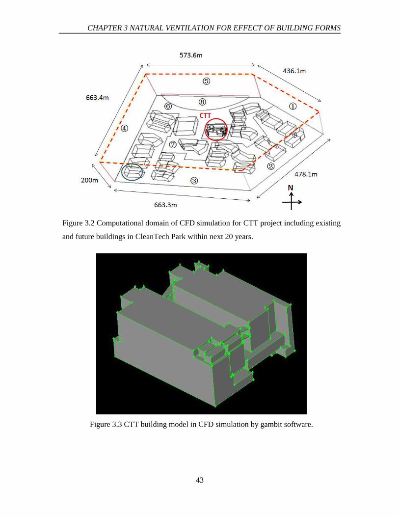
CHAPTER 3 NATURAL VENTILATION FOR EFFECT OF BUILDING FORMS
43
Figure 3.2 Computational domain of CFD simulation for CTT project including existing
and future buildings in CleanTech Park within next 20 years.
Figure 3.3 CTT building model in CFD simulation by gambit software.

CHAPTER 3 NATURAL VENTILATION FOR EFFECT OF BUILDING FORMS
44
Figure 3.4 Diagram of CTT model setup for ventilation simulation.
3.2.1 Description of Model
The computational domain of CFD simulation is shown in Figure 3.2, in which the
domain is made up with eight boundary surfaces, numbered as ①, ②, ③, ④, ⑤, ⑥
(sky), ⑦ (ground), and ⑧ representing a forest located in the north side of CTT. Inside
the domain, the target building CTT with the height of 37.5 m above ground is circled in
red, and the surrounding buildings include one existing building CleanTech One and
other future buildings within next twenty years. The tallest building within the domain is
circled in blue with a height of 38 m.
More detailed CTT model is shown in Figure 3.3. In general it is necessary to use a
mathematical model simplifying for problem simulation with desired accuracy. Based on
these, several assumptions are made and they are:
A flat surface is assumed for the ground.
Most details of CTT are captured except the louvers and green walls.
Simple blocks are used to represent surrounding buildings. Only the shape,
relative height and location are considered, except other details.
Porous structure is used to represent the forest as indicated by ⑧.

CHAPTER 3 NATURAL VENTILATION FOR EFFECT OF BUILDING FORMS
45
As shown in Figure 3.4, the inbound vertical wind profile is given by the
Logarithmic law with the reference height of 15 m.
3.2.2 Boundary Condition
The boundary conditions for CTT model are shown in Table 3.1, in which the locations
of boundaries are shown in Figure 3.2. The boundary conditions vary with wind scenarios,
which are classified into north, northeast, south and southeast wind. In each wind
scenario, the average wind speed indicated in Table 1.2 is used.
Table 3.1 Boundary conditions for CTT model.
Boundary
Wind Scenario
North North &
Northeast South Southeast
①
Velocity Inlet
Wind Speed
m/s 2wind v
Velocity Inlet
Wind Speed = 2.9
m/s
Pressure Outlet
Pressure Outlet
② Pressure Outlet Pressure Outlet Pressure Outlet Pressure Outlet
③ Pressure Outlet Pressure Outlet
Velocity Inlet
Wind Speed = 2.8
m/s
Velocity Inlet
Wind Speed = 3.2
m/s
④ Pressure Outlet Pressure Outlet
Velocity Inlet
Wind Speed = 2.8
m/s
Velocity Inlet
Wind Speed = 3.2
m/s
⑤
Velocity Inlet
Wind Speed = 2
m/s
Velocity Inlet
Wind Speed = 2.9
m/s
Pressure Outlet Pressure Outlet
⑥ Symmetry
⑦ Wall
⑧ Porosity Zone with Inertial Resistance = 0.45 m-1
A porous media is used to simulate the block effect of the forest, based on the inertial loss
coefficient C [50].
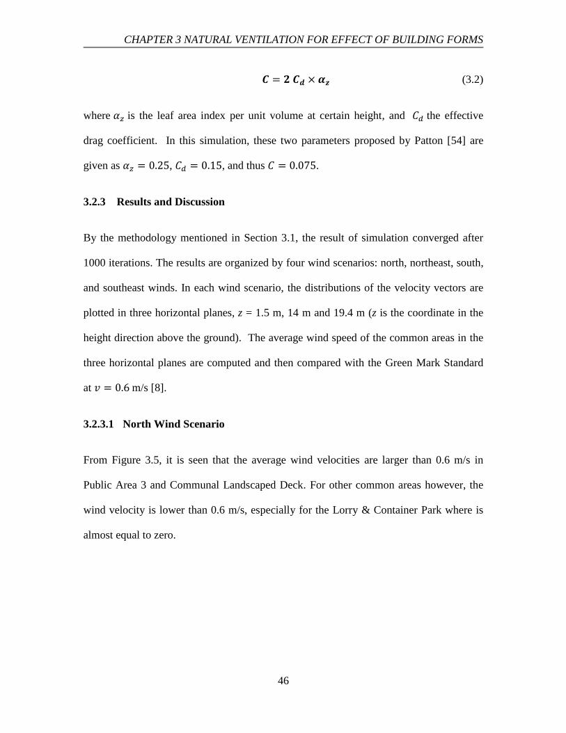
CHAPTER 3 NATURAL VENTILATION FOR EFFECT OF BUILDING FORMS
46
(3.2)
where is the leaf area index per unit volume at certain height, and the effective
drag coefficient. In this simulation, these two parameters proposed by Patton [54] are
given as , , and thus .
3.2.3 Results and Discussion
By the methodology mentioned in Section 3.1, the result of simulation converged after
1000 iterations. The results are organized by four wind scenarios: north, northeast, south,
and southeast winds. In each wind scenario, the distributions of the velocity vectors are
plotted in three horizontal planes, z = 1.5 m, 14 m and 19.4 m (z is the coordinate in the
height direction above the ground). The average wind speed of the common areas in the
three horizontal planes are computed and then compared with the Green Mark Standard
at m/s [8].
3.2.3.1 North Wind Scenario
From Figure 3.5, it is seen that the average wind velocities are larger than 0.6 m/s in
Public Area 3 and Communal Landscaped Deck. For other common areas however, the
wind velocity is lower than 0.6 m/s, especially for the Lorry & Container Park where is
almost equal to zero.

CHAPTER 3 NATURAL VENTILATION FOR EFFECT OF BUILDING FORMS
47
Figure 3.5 Velocity vectors in north wind scenario.
3.2.3.2 Northeast Wind Scenario
From the Figure 3.6, it is observed that the average wind velocities in most common
areas are larger than 0.6 m/s, except the Lorry & Container Park. However, compared
with the north wind scenario, the ventilation situation in the Lorry & Container Park is
improved when wind blows from northeast. The possible reason is that the perpendicular
area is increased between the opening and the wind direction, and thus wind enters this
park much easier.

CHAPTER 3 NATURAL VENTILATION FOR EFFECT OF BUILDING FORMS
48
Figure 3.6 Velocity vectors in northeast wind scenario.
3.2.3.3 South Wind Scenario
From Figure 3.7, it is found that the average wind velocities in most common areas are
lower than 0.6 m/s, except the Public Area 3. Compared with north wind scenario, natural
ventilation situation in all the common areas becomes worse. The possible reason is that
the wild field helps to accelerate the north wind, where the area is outside of the blue box
but within the dark green box, as illustrated in Figure 3.8.

CHAPTER 3 NATURAL VENTILATION FOR EFFECT OF BUILDING FORMS
49
Figure 3.7 Velocity vectors in south wind scenario.
Figure 3.8 Site plan of Clean Tech Park.

CHAPTER 3 NATURAL VENTILATION FOR EFFECT OF BUILDING FORMS
50
3.2.3.4 Southeast Wind Scenario
From Figure 3.9, it is concluded that the average wind velocities in most common areas
are lower than 0.6 m/s, except the Public Area 3 and Communal Landscaped Deck.
Compared with the south wind scenario, the ventilation situation on all the common areas
becomes better, especially the Communal Landscaped Deck. The possible reason is that
the perpendicular area increases between the opening and the wind direction, and wind
can enter this park much more easily.
Figure 3.9 Velocity vectors in southeast wind scenario.

CHAPTER 3 NATURAL VENTILATION FOR EFFECT OF BUILDING FORMS
51
3.2.4 Summary
From all the above four wind scenarios, the average wind speeds in all the public areas
are summarized in Table 3.2. It is clearly shown that Public Area 3 and Communal
Landscaped Deck have good natural ventilation, compared with the Green Mark Standard
0.6 m/s [9].
Table 3.2 Average wind speed for all the public areas in CTT.
Average Speed (m/s) North Wind Northeast Wind South Wind Southeast Wind
Public Area 1 0.2 0.6 0.2 0.25
Public Area 2 0.3 0.8 0.2 0.3
Public Area 3 0.8 0.7 1 1.2
Lorry Park & Container Park 0.1 0.4 0.3 0.4
Communal Landscaped Deck 0.75 1.8 0.4 2
As different wind scenarios have different frequencies stated in Table 1.2, the average
wind speed is obtained as
4
1
Velocity Average )(i
ii FVV (3.3)
where Vi is the wind speed of certain wind scenario in a certain cell, Fi the frequency of
the certain wind scenario, and VAverage Velocity the average wind speed in a certain cell in a
year. After combining four wind scenarios via Eq. (3.3), the results are shown in Figure
3.10.
It is clearly seen that the middle part of rooftop on the south block has higher average
wind velocity of 2 ~ 2.5 m/s. The communal landscaped deck and Public Area 3 have
good ventilation where the average wind velocity is larger than Green Mark Standard of

CHAPTER 3 NATURAL VENTILATION FOR EFFECT OF BUILDING FORMS
52
0.6 m/s [9], while the ventilation in other public areas needs to be improved, where the
average wind velocity is lower than 0.6 m/s.
Figure 3.10 Average wind velocity in a year.

CHAPTER 3 NATURAL VENTILATION FOR EFFECT OF BUILDING FORMS
53
3.3 Project II: A Porous Academic Building North Spine Academic
Building
Normally the word “porous” is used to describe a material which has many holes inside.
However, now it is extended to describe a building which has may void inside and such
voids help to enhance the natural ventilation. According to the master plan of NTU
published in 2012, there will be ten new buildings in the campus in the next several years.
One of them is the North Spine Academic Building (NSAB) illustrated in Figure 3.11.
NSAB is right now in design phase and the target of this project is to achieve as much as
40% energy saving. Therefore, natural ventilation becomes attractive as one of the energy
saving strategies in the design stage, which building can be enhanced further by
increasing the porosity.
Figure 3.11 Impression drawing of NSAB building (Source: ADDP).

CHAPTER 3 NATURAL VENTILATION FOR EFFECT OF BUILDING FORMS
54
Figure 3.12 Computational domain of the NSAB model
Figure 3.13 Top view of NSAB and neighbor buildings in CFD simulation model.
3.3.1 Description of Model
NSAB is a seven-storey building with the ground floor named as “Basement Four (B4)”
and the other levers from bottom to top are “Basement Three (B3)”, “Basement Two
(B2)”, “Basement One (B1)”, “Level One (L1)”, “Level Two (L2)” and “Level Three
(L3)”.
The simulation model is shown in Figures 3.12and 3.13. The neighboring buildings, N4,
N3, N4.1 and LT 2A, are included and NSAB is circled in red. Inside NSAB, all the
①
③
② ④
⑤
⑥

CHAPTER 3 NATURAL VENTILATION FOR EFFECT OF BUILDING FORMS
55
toilets are designed in a naturally ventilation manner. In order to simulate the NSAB
model, the following assumptions are made:
A flat surface is assumed for the ground, but the height differences between the
buildings are considered.
The toilets are naturally ventilated, and the screen inside the toilets has 50%
porosity.
Simple blocks are used to represent surrounding buildings, N3, N4, N4.1 and LT
2A.
As shown in Figure 3.4, the inbound vertical wind profile is given by the
Logarithmic law with reference height of 15 m.
k-ε realizable turbulence model is used with the backflow turbulent intensity of 5%
and viscosity ratio of 5% [55].
For the solar radiation model, Solar Ray Tracing model [56] is engaged with
Longitude of 103.667 °, Latitude of 1.35 ° and Time Zone 8.
13:00 pm on 21st June is chosen as the simulation time, when the solar intensity is
the highest within a day.
The solar irradiation value and outside temperature are from epw file of energy
simulation.
3.3.2 Boundary Conditions
The boundary conditions are shown in Table 3.3, in which the locations of boundaries are
shown in Figure 3.12. The boundary conditions vary with wind scenarios, which are
classified into north, northeast, south and southeast wind. In each wind scenario, the
average wind speed indicated in Table 1.2 is used.

CHAPTER 3 NATURAL VENTILATION FOR EFFECT OF BUILDING FORMS
56
Table 3.3 Boundary conditions for CFD simulation of NSAB.
Boundary Wind Scenarios
North Wind Northeast Wind South Wind Southeast Wind
①
Velocity Inlet
Wind Speed = 2
m/s
Velocity Inlet
Wind Speed = 2.9
m/s
Pressure Outlet Pressure Outlet
② Pressure Outlet
Velocity Inlet
Wind Speed = 2.9
m/s
Pressure Outlet
Velocity Inlet
Wind Speed = 3.2
m/s
③ Pressure Outlet Pressure Outlet
Velocity Inlet
Wind Speed = 2.8
m/s
Velocity Inlet
Wind Speed = 3.2
m/s
④ Pressure Outlet Pressure Outlet Pressure Outlet Pressure Outlet
⑤ Symmetry Symmetry Symmetry Symmetry
⑥ Wall Wall Wall Wall
Screen
inside the
toilets
Pressure Jump
50% porosity
3.3.3 Results and Discussion
Based on the methodology mentioned in Section 3.1 of this chapter, the simulation result
is converged after 1000 iterations. The results are organized by four wind scenarios: north
wind, northeast wind, south wind and southeast wind, as detailed in the following sub-
sections. In each wind scenario, both the plane and cross-sectional views of velocity
contour are plotted at all seven levels, in which the average wind speed of the common
areas in three horizontal planes are computed and then compared with the Green Mark
Standard (0.6 m/s) [9].

CHAPTER 3 NATURAL VENTILATION FOR EFFECT OF BUILDING FORMS
57
3.3.3.1 North Wind Scenario
From Figures 3.14 and 3.15, it is seen that the wind has the highest speed in Basement
Four compared with the other levels, and it achieves its maximum speed at about 2.7 m/s
inside the common space of Basement Four. One possible reason is the tunneling effect,
and the other is that Basement Four has big opening in neighbor buildings, such that the
wind can easily enter NSAB. The wind speed in Levels 1 to 3 is the lowest compared
with that in other levels. The wind speed inside the small atrium is about 0.1~1.2 m/s.
3.3.3.2 Northeast Wind Scenario
From Figures 3.16 and 3.17, it is observed that the whole wind flow pattern is similar to
that in north wind scenario. The only difference is that the wind speed everywhere is
increased.
3.3.3.3 South Wind Scenario
From Figures 3.18 and 3.19, it is found that the wind pattern in south wind scenario is
very similar to that in north and northeast wind scenarios, but the wind speed everywhere
is larger than that in north wind scenario, but smaller than that in northeast wind scenario.
3.3.3.4 Southeast Wind Scenario
From Figures 3.20 and 3.21, it is concluded that the wind pattern in south wind scenario
is very similar to that in north, northeast and south wind scenarios, but the wind speed
everywhere is the largest among these four wind scenarios.

CHAPTER 3 NATURAL VENTILATION FOR EFFECT OF BUILDING FORMS
58
Figure 3.14 Plane view of velocity contour of seven levels within NSAB under north
wind scenario.
Figure 3.15 Cross section view: (a) cross section line; (b) velocity vector within the
small atrium area; (c) velocity contour.

CHAPTER 3 NATURAL VENTILATION FOR EFFECT OF BUILDING FORMS
59
Figure 3.16 Plane view of velocity contour of seven levels within NSAB in northeast
wind scenario.
Figure 3.17 Cross section view: (a) cross section line; (b) velocity vector within the
small atrium area; (c) velocity contour.

CHAPTER 3 NATURAL VENTILATION FOR EFFECT OF BUILDING FORMS
60
Figure 3.18 Plane view of velocity contour of seven levels within NSAB in south wind
scenario.
Figure 3.19 Cross section view: (a) cross section line; (b) velocity vector within the
small atrium area; (c) velocity contour.

CHAPTER 3 NATURAL VENTILATION FOR EFFECT OF BUILDING FORMS
61
Figure 3.20 Plane view of velocity contour of seven levels within NSAB in southeast
wind scenario.
Figure 3.21 Cross section view: (a) cross section line; (b) velocity vector within the
small atrium area; (c) velocity contour.

CHAPTER 3 NATURAL VENTILATION FOR EFFECT OF BUILDING FORMS
62
3.3.4 Summary
Thermal comfort inside the small atrium is calculated based on PMVNV-PPD model and
shown in Table 3.4. It is shown that for southeast wind scenario, the situation is very
good, where percentage of satisfaction (PS) is about 90%. However, PS is only 49% for
northeast wind scenario. Thermal comfort inside toilets is not good, where PS is less than
10% for all the toilets.
Table 3.4 Area-weighted average wind speed and percentage of thermal comfort inside
the common spaces in seven levels for four wind scenarios.
NE-Wind SE-Wind N-Wind S-Wind
Velocity
(m/s)
PS
(%)
Velocity
(m/s)
PS
(%)
Velocity
(m/s)
PS (%) Velocity
(m/s)
PS (%)
L3 1.74 66.9 1.79 84.1 0.67 16.19 1.01 56.34
L2 1.61 56.7 1.79 75.9 0.63 9.81 0.72 32.31
L1 1.88 49.2 2.42 73.8 0.66 7.35 0.75 29.83
B1 2.03 61.8 2.18 59.6 0.89 15.92 1.13 48.45
B2 1.97 56.0 2.70 56.3 0.73 7.04 1.09 43.49
B3 1.87 45.0 1.82 54.5 0.7 2.19 0.93 29.83
B4 2.97 63.2 3.09 50.7 1.33 11.01 1.86 59.63
Toilets <10 <10 <10 <10
3.4 Project III: A Free-Form Academic Building Learning Hub
The new Learning Hub (LH) is one of fourteen new buildings at NTU within the next
three years, under the University’s Campus Master Plan that will transform the NTU
campus into a University City. LH broke ground on 12th
October 2012, and currently it is
under construction.

CHAPTER 3 NATURAL VENTILATION FOR EFFECT OF BUILDING FORMS
63
This hub has nine stories with total height of 34.2 m, and each level has the height of 3.8
m. It is designed with a structure without conventional corridors. As a flower like layout,
it is made up of several “petals” (involving 55 tutorial rooms), atrium and 3 staircase
blocks, as shown in Figure 3.22. In Level 1, there are only petals in the north, south and
west side. From Level 2 to Level 6, there are 13 petals. In Levels 7 to 9, there are 10, 6
and 4 petals respectively. It also allows the students to enter from all directions around
into a large central space which links all the separate “petals” together. Each “petal”
tower consists of classrooms and is build up gradually. Gardens, shaded terraces, and
pergolas are designed on selected upper levels and rooftops, as shown in Figure 3.22. All
the rooms are air-conditioned. On the other hand, the public spaces (e.g. the corridors and
atrium area) are designed to be naturally ventilated.
Figure 3.22 Impression drawing of LH building. (Source: NTU)

CHAPTER 3 NATURAL VENTILATION FOR EFFECT OF BUILDING FORMS
64
3.4.1 Description of Model
The computational domain for LH model is shown in Figure 3.23, in which the domain is
made up of six boundary surfaces, numbered as ①, ②, ③, ④, ⑤ (sky), and ⑥
(ground). Inside the domain, LH with building height of 34.2 m and three nearest
neighbor buildings, Business school with building height 1.9 m lower than LH, School of
Humanities and Social Sciences (HSS) with building height 12.5 m lower than LH and
Innovation Center (26.45 m lower than LH) are considered in this simulation.
As shown in Figure 3.24, this is a nine story building with each level height of 3.8 m, and
formed by 13 blocks and the interconnected “corridors”. Only the individual rooms are
air-conditioned; the corridors and atrium areas are designed to be naturally ventilated.
The staircases are with 50% porosity which enhances the natural ventilation in the atrium
and corridors. The detailed LH model in CFD simulation is shown in Figure 3.25. In
order to build up the simulation model, there are some assumptions:
The ground is assumed to be a flat surface, but the height difference between LH
and surrounding buildings are considered.
Simple blocks are used to represent surrounding buildings, HSS, Innovation
Center and Business School.
The shapes of all Learning Hub blocks from Level 2 to Level 9 are assumed to be
the same, but all the other details are considered.
The envelopes of staircases of LH have 50% porosity.
As shown in Figure 3.4, the inbound vertical wind profile is given by the
Logarithmic law with the reference height of 15 m.
Turbulence model and solar ray tracing model is the same as that in NSAB project.

CHAPTER 3 NATURAL VENTILATION FOR EFFECT OF BUILDING FORMS
65
Figure 3.23 Computational domain for LH model
Figure 3.24 Cross section view of LH model.

CHAPTER 3 NATURAL VENTILATION FOR EFFECT OF BUILDING FORMS
66
Figure 3.25 Top view of LH model in CFD simulation.
Figure 3.26 Cross section view (Level 5) of LH building model in which gaps and
staircases together with four selected measured points are shown.

CHAPTER 3 NATURAL VENTILATION FOR EFFECT OF BUILDING FORMS
67
3.4.2 Boundary Conditions
The boundary conditions for LH model is shown in Table 3.5, in which the locations of
boundaries are shown in Figure 3.23. The boundary conditions vary with wind scenarios,
which are classified into north, northeast, south and southeast wind. In each wind
scenario, the average wind speed indicated in Table 1.2 is used. To simulate the envelope
of staircases which have porosity of 50%, Porous Jump model [57] is used. Porous jump
conditions are normally used to model a thin "membrane'' that has pressure-drop
characteristics. In this Porous Jump mode, there are two important parameters, the
thickness of the “membrane” and the pressure jump coefficient which define the pressure
drop over this “membrane”.
Table 3.5 Boundary conditions for Learning Hub natural ventilation simulation.
Boundary North Wind Northeast Wind South Wind Southeast Wind
① Velocity Inlet
Wind Speed = 2
m/s
Velocity Inlet
Wind Speed = 2.9
m/s
Pressure Outlet Pressure Outlet
② Pressure Outlet Velocity Inlet
Wind Speed = 2.9
m/s
Pressure Outlet Velocity Inlet
Wind Speed = 3.2
m/s
③ Pressure Outlet Pressure Outlet Velocity Inlet
Wind Speed = 2.8
m/s
Velocity Inlet
Wind Speed = 3.2
m/s
④ Pressure Outlet Pressure Outlet Pressure Outlet Pressure Outlet
⑤ Symmetry Symmetry Symmetry Symmetry
⑥ Wall Wall Wall Wall
Envelopes of
Staircases
Porous Jump
Thickness: 0.1 m;
Pressure-Jump Coefficient: 31.24 m-1

CHAPTER 3 NATURAL VENTILATION FOR EFFECT OF BUILDING FORMS
68
3.4.3 Results and Discussion
Based on the methodology mentioned in Section 3.1 of this chapter, the simulation result
converged after 1000 iterations. The results are organized by wind directions: north wind,
northeast wind, south wind and southeast wind. In each wind scenario, the contours of
static pressure and velocity vectors are provided. All the results are based on the
horizontal plane which is 1.5 meters height above the floor. The reason for choosing such
plane is that 1.5 meter height is the height of people activities.
In all the figures below, z is the coordinate of height. For example z = 1.5 m means that
the height of the plane is 1.5 m above the ground. Similarly, z = 31.9 m means that the
plane is 31.9 m above the ground. All the circled areas in light blue are the blocks of LH
building. The area surrounded by these blocks is the atrium area, which is interested for
natural ventilation.
3.4.3.1 North Wind Scenario
From Figure 3.27, it is clearly seen that from Level 1 to 2, the maximum wind velocity in
the atrium area decreases, and the areas with wind velocity larger than 0.6 m/s [8]
decrease. This is because the size of blocks increases and the distance between blocks
decrease, so it reduces the possibility of wind entering into the atrium area. From Level 2
to 6, the wind profiles are almost the same.
From Level 6 to 7, the area with wind velocity larger than 0.6 m/s increases. There are
two possible reasons for this situation. One is that some blocks are removed compared to
Level 6. The other is that the HSS building is located in the northeast of LH and is 12.5 m

CHAPTER 3 NATURAL VENTILATION FOR EFFECT OF BUILDING FORMS
69
lower than LH, meaning that the effect of wind blockage due to HSS building almost
disappears from Level 7 and above.
The major difference between Level 7 and 8 is that the block located in the north is
removed, so that a good channel is created for cross ventilation. This situation also
happens in Level 9. However, the average wind velocity in Level 9 increases compared
that in Level 8. This is because that the Business School Building located in the
northwest of LH is 1.7 m lower than LH, meaning that the blockage effect due to
Business School almost disappears from level 9.
Figure 3.27 Velocity vectors of 9 floors for north wind scenario.
N

CHAPTER 3 NATURAL VENTILATION FOR EFFECT OF BUILDING FORMS
70
Figure 3.28 Circulation winds in between the buildings.
3.4.3.2 Northeast Wind Scenario
Similar to North Wind Scenario, from Level 1 to Level 2, the maximum wind velocity in
the atrium area decreases and the areas with wind velocity larger than 0.6 m/s decrease
largely, as shown in Figure 3.29 This is because that the size of blocks increases and the
distance between blocks decreases; as a result it reduces the possibility of wind entering
into the atrium area.
It is found that there is almost no wind from Level 2 to Level 4 in northeast wind scenario,
which is very different from north wind scenario. This is due to the blockage effect of
HSS building. The wind blows from northeast and HSS is located just in the northeast of
Learning Hub. Such blockage effect of HSS is much bigger than that in the north wind
scenario. In Level 5 and 6, there are some winds, although the blockage effect of HSS
still exists. One possible reason is the circulations of wind in between buildings when
wind blows from lower building to higher building, as illustrated in Figure 3.28. Such
circulation enables the wind to blow through the gaps in between the blocks.

CHAPTER 3 NATURAL VENTILATION FOR EFFECT OF BUILDING FORMS
71
The reasons for the difference between Level 6 and 7 are the same as that in north wind
scenario. One is that some blocks are removed compared with Level 6. The other is that
the effect of wind blockage almost disappears due to HSS building. In Level 7, a channel
for cross ventilation is created by removing two blocks. Similarly, another channel for
cross ventilation is created in Level 8 by removing one north block.
It is found that the average wind velocity in Level 9 increases compared that with Level 8
in northeast wind scenario, which is similar to north wind scenario. The possible reason is
that blockage effect due to Business School almost disappears from Level 9.
Figure 3.29 Velocity vectors of 9 floors for northeast wind scenario.
N

CHAPTER 3 NATURAL VENTILATION FOR EFFECT OF BUILDING FORMS
72
3.4.3.3 South Wind Scenario
The flow patterns of Level 2 and 3 are almost the same, as shown in Figure 3.30. The
wind flow patterns of Level 4, 5 and 6 are almost the same. From Level 7 to 9, areas with
velocity larger than 0.6 m/s increases. The possible reason is that some blocks are
removed, which results in enhancing the cross ventilation.
Figure 3.30 Velocity vectors of 9 floors for south wind scenario.
N

CHAPTER 3 NATURAL VENTILATION FOR EFFECT OF BUILDING FORMS
73
3.4.3.4 Southeast Wind Scenario
The wind flow patterns of Level 3, 4, 5 and 6 are almost the same. From Level 7 to 9,
areas with velocity larger than 0.6 m/s increases. The possible reason is that some blocks
are removed, which results in enhancing the cross ventilation.
Figure 3.31 Velocity vectors of 9 floors for southeast wind scenario.
3.4.4 Summary
Based on the discussions above, several conclusions are made as follows. (1) North wind
scenario is the worst among four wind scenarios. This is mainly due to the blockage
effect by the Business school. (2) In Level 2 to 6, the ventilation is very bad especially
for the north and northeast wind scenarios.
N

CHAPTER 3 NATURAL VENTILATION FOR EFFECT OF BUILDING FORMS
74
The percentage of areas with velocity greater than 0.6 m/s is shown in Table 3.6. It is
shown that the best situation of natural ventilation in the atrium occurs when southeast
wind prevails. This always happens from June to September in Singapore, when 47.2% of
total atrium area are natually ventilated. The worst case happens when north wind
prevails, which always happens from December to March. In this case, the atrium areas
from Level 2 to Level 7 are totally not naturally ventilated at all.
Table 3.6 Percentage of comfort areas.
Levels North Wind Northeast Wind South Wind Southeast Wind
Level 1 5 % 10 % 35% 60%
Level 2~Level 6 0 % Level 2~4: 0%
Level 5: 3 %
Level 6: 5%
20% 20%
Level 7 0 % 50% 75% 80%
Level 8 20% 70% 75% 95%
Level 9 30% 70% 80% 90%

CHAPTER 4 BUILDING ENERGY SIMULATION
75
CHAPTER 4 ENERGY EFFICIENCY FOR EFFECT
OF BUILDING ENVELOPE
In general, there are three most commonly-used architectural shading designs in buildings,
namely the external overhang design, vertical greenery shading, and internal venetian
blind. In this chapter therefore, the three shading envelope designs are studied via energy
and CFD simulations: (1) external building envelope including the plane-plate and
curved-shell envelopes, (2) the vertical green envelope, and (3) internal smart blind. The
building energy simulation is conducted by the EnergyPlus-based software, OpenStudio,
in order to study the effect of various building envelope parameters on the indoor cooling
load, due to the external building and vertical green envelopes respectively. For analysis
of effect of the internal venetian blind, the CFD simulation software, Fluent, is used for
modeling and simulation of the temperature profile inside the building.
4.1 Methodology for Simulation of Building Energy
OpenStudio is an open source software for modeling and simulation of building energy,
developed by National Renewable Energy Laboratory (NREL), in order to simulate
building energy based on EnergyPlus and carry out the advanced daylight analysis based
on Radiance. A graphical energy-modeling tool, OpenStudio, includes the functions of
visualization, and schedules editing, loads constructions and materials editing, a drag and
drop interface to make input of resources for spaces and zones, a visual HVAC and
service water heating design tool, and output visualization. In the present work,
OpenStudio is used to simulate the building energy consumption for various types of
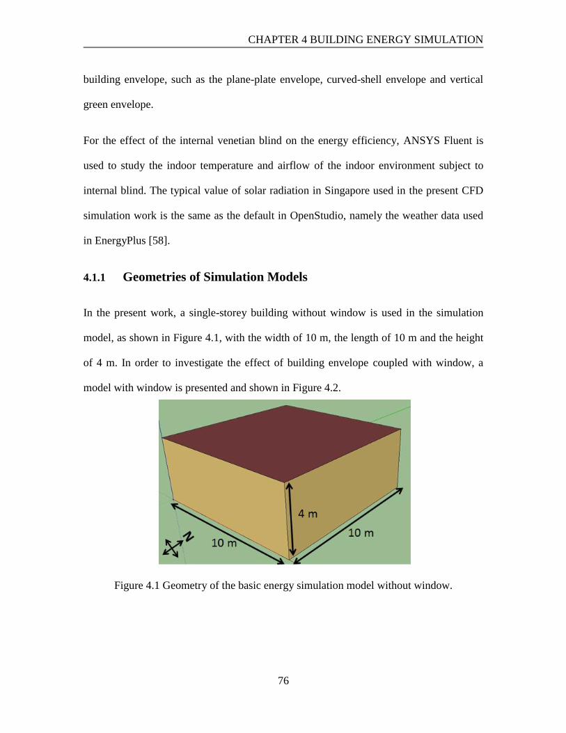
CHAPTER 4 BUILDING ENERGY SIMULATION
76
building envelope, such as the plane-plate envelope, curved-shell envelope and vertical
green envelope.
For the effect of the internal venetian blind on the energy efficiency, ANSYS Fluent is
used to study the indoor temperature and airflow of the indoor environment subject to
internal blind. The typical value of solar radiation in Singapore used in the present CFD
simulation work is the same as the default in OpenStudio, namely the weather data used
in EnergyPlus [58].
4.1.1 Geometries of Simulation Models
In the present work, a single-storey building without window is used in the simulation
model, as shown in Figure 4.1, with the width of 10 m, the length of 10 m and the height
of 4 m. In order to investigate the effect of building envelope coupled with window, a
model with window is presented and shown in Figure 4.2.
Figure 4.1 Geometry of the basic energy simulation model without window.

CHAPTER 4 BUILDING ENERGY SIMULATION
77
Figure 4.2 Geometry of basic energy simulation model with window on east wall.
4.1.1.1 Plane-Plate Envelope
For the effect of geometry of the plane-plate envelope on energy efficiency, three
parameters are studied in details via modeling and simulation. They are the length of
building envelop (L), the distance between the building envelope and wall (D), and the
angle of the building envelope and wall (θ), as shown in Figure 4.3. In addition, the
building height (H) is used to normalize the parameters L and D. In the present numerical
simulations, the L/H ranges from 0 to 1, D/H from 0 to 1, and θ from 0° to 90°.
Figure 4.3 Geometric parameters of plane-plate envelope.

CHAPTER 4 BUILDING ENERGY SIMULATION
78
4.1.1.2 Curved-Shell Envelope
For the curved-shell building envelope, there are two commonly-used positions: the
horizontal overhang and vertical envelope, as shown in Figure 4.4. For analysis of the
effect of geometry of curved shell envelope on energy efficiency, two parameters are
studied in details via modeling and simulation. They are the length of building envelop (L)
for the horizontal overhang design, and the distance between the building envelope and
wall (D) for the vertical envelope design.
Figure 4.4 Geometric parameters of curved-shell envelope for the effect on building
energy efficiency in the vertical envelope design (a) and the horizontal overhang design
(b).

CHAPTER 4 BUILDING ENERGY SIMULATION
79
4.1.1.3 Vertical Green Envelope
For the effect of vertical green envelope on the building energy efficiency, a porous
model is used to simulate its shading effect by capturing the porosity ratio of the whole
vertical green envelope. The porosity ratio is the ratio between area of hole and area of
whole envelope and varies from 0 to 1, whereby 0 means there is no holes on the
envelope and 1 means there is no envelope. The simulation models of vertical envelope
with different porosity ratio are shown in Figure 4.5, in which the distance between the
vertical green envelope and building wall is constant in order to focus on the effect of
porosity ratio. In the present model, the distance between the vertical green envelope and
building wall is 1m which is referred to as the Clean Tech One building.
In order to investigate the correlation of vertical green envelope and window in terms of
building energy efficiency, here with-window and windowless scenarios are carried out.
In each scenario, there are 9 simulation models with porosity ratio 10%, 20%, 30%, 40%,
50%, 60%, 70%, 80% and 90%. Figure 4.6 shows the simulation model of vertical green
envelope with 50% porosity.

CHAPTER 4 BUILDING ENERGY SIMULATION
80
Figure 4.5 Geometry of simulation models with vertical green envelope which has
porosity ratio of 10% (a), 20% (b), 30% (c), 40% (d), 50% (e), 60% (f), 70% (g), 80%
(h) and 90% (i).
Figure 4.6 Geometry of simulation models with vertical green envelope with 50%
porosity ratio for building with window (a) and windowless building (b).

CHAPTER 4 BUILDING ENERGY SIMULATION
81
4.1.1.4 Internal Smart Blind
For the effect of internal smart blind on building energy efficiency, Fluent is used to
simulate the indoor temperature and airflow. Compared with static blind, the smart blind
can adjust its tilt angle to face directly towards the sun, according to the sun’s elevation
angle by communicating with the luminance sensor. In the case of rainy days, the
humidity sensor is involved as well.
The simulation model is shown in Figure 4.7, in which the room is a cubic box of 1.5 ×
1.5 × 2 m3, and the blind has a length of 1.5m, width of 0.05 m and thickness of 0.003 m.
The distance between two neighbor blinds is 0.05m meaning that, when the blinds are
closed, there is no gap between the two neighbor blinds. In the present simulation work,
the west wall of the building is a window made up of glass material and other walls are
made up with concrete.
Figure 4.7 Geometry of simulation model with internal smart blind.

CHAPTER 4 BUILDING ENERGY SIMULATION
82
The blind tilt angle is calculated based on the vector of solar incident ray which is
calculated by solar calculator in ANSYS Fluent and shown in Table 4.1 From the blind
title angle, the vertical distance of gap between two neighbor blinds can be calculated.
Since the window is located on the west façade, the direct solar radiation can only enter
into the building during the afternoon time from 1:00 pm to 6:00 pm. Therefore, the
smart blind is fully opened from 8:00 am to 12:00 pm.
Table 4.1 Blind tilt angle and openness factor calculated based on vector of solar incident
ray.
Time
Vector of solar incident ray Blind Tilt
Angle (°)
Vertical
Blind Gap
Distance
(cm)
Openness
Factor x y z
8:00 am -0.3924003 0.8916435 0.2258182 90 5 100%
9:00 am -0.3870584 0.8056033 0.4485411 90 5 100%
10:00 am -0.3827416 0.6681235 0.6380594 90 5 100%
11:00 am -0.3788352 0.4784777 0.7921761 90 5 100%
12:00 pm -0.3765128 0.2596771 0.8892727 90 5 100%
1:00 pm -0.3756232 0.02318264 0.9264825 68 3.12 62%
2:00 pm -0.3765139 -0.2100136 0.9022924 64 2.84 57%
3:00 pm -0.3782829 -0.4383183 0.8153399 55 2.11 42%
4:00 pm -0.381805 -0.628249 0.677885 43 1.32 26%
5:00 pm -0.3861023 -0.7824106 0.4886294 29 0.64 13%
6:00 pm -0.3913333 -0.8796299 0.2703876 16 0.19 4%
4.1.2 Assumption and input of Simulation Model
For modeling of the plane-plate, curved-shell and vertical green envelope, OpenStudio
software is used with the default model of AHARE Medium Office [59]. In the Medium
Office model, the default values are used to simulate the cooling load, as shown in Table

CHAPTER 4 BUILDING ENERGY SIMULATION
83
4.2, in which the density of people is given as 0.054 people/m2, the density of lighting
energy 9.688 W/m2, the plug load 5.813 W/m
2, and air infiltration rate 0.150 h
-1. As well
known, the total indoor cooling load consists of two parts, the sensible load and latent
loads. In this thesis, sensible load refers to the sensible heating gains from outdoor
environment through convection, conduction or solar radiation, and latent load refers to
the latent heat gains from outdoor environment when moisture is added to the space by
means of vapor emitted by the occupants or generated by a process or through air
infiltration. It is thus assumed that the human body contributes to the sensible and latent
loads, and the equipment and lighting contribute to the sensible load only.
Table 4.2 Cooling load contribution for energy simulation
Contribution
Factors
People density
(people/m2)
Plug load
(W/m2)
Lighting load
(W/m2)
Air infiltration
rate (h-1
)
Energy density 0.054 5.813 9.688 0.150
In order to simulate the one-year energy consumption, the schedules are assumed as
follows, which are applicable for simulation of the plane-plate envelope, the curved-shell
envelope and the vertical green envelope. In general, the schedules include three main
activities for the simulation model, namely the schedule of lighting system, the schedule
of occupancy, and the schedule of equipment, as shown in Figures 4.8 to 4.13. Inside
these figures, the y-axis represents the normalized value from 0 to 1. In Figure 4.8, for
example, the value of y-axis is 0.86 at 8:00 am, meaning that the lighting load is 86% of
the maximum lighting load.

CHAPTER 4 BUILDING ENERGY SIMULATION
84
4.1.2.1 Schedule of Lighting System
Figure 4.8 Schedule of lighting system on weekdays.
Figure 4.9 Schedule of lighting system on Saturday.
The schedule of lighting system used in the study is the default value in OpenStudio. The
lighting system is turned off on Sunday and turned on during weekdays and Saturday, as
shown in Figures 4.8 and 4.9 respectively. During weekdays, the lighting is turned on
starting from 5:00 am and turned off after 11:00 pm, and the peak load starts from 8:00
am to 5:00 pm. On Saturday, the lighting is turned on starting from 6:00 am and turned
off after 5:00 pm, and the peak load starts from 8:00 am to 2:00 pm.

CHAPTER 4 BUILDING ENERGY SIMULATION
85
4.1.2.2 Schedule of Occupancy
Figure 4.10 Schedule of occupancy on weekdays.
Figure 4.11 Schedule of occupancy on Saturday.
The schedule of occupancy used in this study is the default value in OpenStudio. People
do not come to the building on Sunday and come to work during weekdays and Saturday
shown in Figures 4.10 and 4.11 respectively. During weekdays, the people start to come
to office from 6:00 am and leave after 10:00 pm, and from 8:00 am to 5:00 pm all the
people are assumed in the office except of the lunch time from 12:00 pm to 1:00 pm. On
Saturday, 50% of people come to the office since 8:00 am and leave after 2:00 pm.

CHAPTER 4 BUILDING ENERGY SIMULATION
86
4.1.2.3 Schedule of Equipment
Figure 4.12 Schedule of equipment on weekdays.
Figure 4.13 Schedule of equipment on Saturday.
The schedule of equipment used in this study is the default value in OpenStudio. It is
assumed that the equipment is partially turned on during weekdays and Saturday, and
turned off on Sunday, as shown in Figures 4.12 and 4.13 respectively. During weekdays,
the percentage of the equipment in usage increases from 40% to 86% from 6:00 am to
8:00 am, and then remains 80% until 5:00 pm except of lunch time from 12:00 pm to
1:00 pm. Then it starts to decrease after 5:00 pm and returns to 40% from 11:00 pm. On
Saturday, the percentage of the equipment in usage increases from 30% to 50% in the

CHAPTER 4 BUILDING ENERGY SIMULATION
87
period between 6:00 am and 8:00 am and starts to decrease after 2:00 pm, and then
returns to 30% after 5:00 pm.
4.1.2.4 Assumptions and Inputs for CFD Simulation
For modeling of internal smart blind, Fluent is engaged to simulate the internal
temperature and airflow with or without smart blind or with static blind. The solar load
model in Fluent is engaged to calculate radiation effects from the sun ray that enters the
computational domain. The solar load model includes a solar calculator utility that can be
used to construct the sun's location in the sky for a given time-of-day, date, and position.
As for the ventilation, k-ε renormalization group theory (RNG) model is used to capture
the buoyance driven ventilation inside the building.
Following assumptions are made for the present CFD simulation:
It is assumed that no air-conditioning is provided inside the building.
The shading effect from neighbor buildings is not considered, in order to focus on
the effect of smart blind on building energy efficiency.
For Benchmark D mentioned in 4.1.3 Post Process, the static blind is assumed to
be flat all the time.
The solar radiation intensity value and outdoor temperature used in the CFD simulation is
shown in Table 4.3. Diffuse solar radiation is due to the sunlight that has been scattered
by molecules and particles in the atmosphere, while direct radiation comes from the sun
on a cloudless day.

CHAPTER 4 BUILDING ENERGY SIMULATION
88
Table 4.3 Solar radiation intensity and outdoor temperature in Singapore on 21st June [51].
Time
Global
horizontal
radiation (W/m2)
Direct normal
radiation (W/m2)
Diffuse radiation
(W/m2)
Dry Bulb
Temperature (°C)
8:00 am 22 0 22 27.4
9:00 am 149 59 129 29
10:00 am 305 106 246 29
11:00 am 442 95 373 29.8
12:00 pm 542 107 451 31
1:00 pm 597 193 420 31
2:00 pm 601 192 424 29.2
3:00 pm 628 280 386 30
4:00 pm 570 345 312 30
5:00 pm 435 375 215 30.6
6:00 pm 226 196 151 30
The boundary conditions in the present CFD simulation are shown in Table 4.4. Except
that the west wall is made up with glass that is semi-transparent, the other walls are made
up with concrete that is opaque. The U value is calculated based on Equations 2.3 to 2.4
and listed in Table 4.5. As for all the materials used in the CFD simulation, the material
properties are shown in Table 4.5 including the density, specific heat and thermal
conductivity.
Table 4.4 Boundary conditions in CFD simulation.
Boundary
Condition
Boundary
Condition Materials Thickness (m)
U value
(W/(m2·K))
East Wall Opaque Concrete 0.21 1.6756
North Wall Opaque Concrete 0.21 1.6756
South Wall Opaque Concrete 0.21 1.6750
Roof Wall Opaque Concrete 0.25 0.5277
Ground Wall Opaque Concrete 0.21 2.1305
West Wall Semi-Transparent Glass 0.006 5.2800
Blind Wall Opaque Aluminium 0.003 6.0970

CHAPTER 4 BUILDING ENERGY SIMULATION
89
Table 4.5 Material properties used in CFD simulation [12].
Concrete Carpet Glass Aluminium Building Insulation
Density (kg/m3) 2400 288 2220 2719 10
Specific Heat (J/kg·K) 750 1380 830 871 830
Thermal Conductivity
(W/(m·K)) 1.442 0.06 1.15 202.4 0.1
4.1.3 Post Process
For analysis of building energy consumption, the post process of energy simulation is
conducted. Here the final indoor district cooling load with unit of Giga-Joule (GJ) is used
as a key parameter for comparison and analysis of the effect of various envelope
parameters. In order to study the improvement by adding the external building envelope,
two benchmark models are used in the study: Benchmark A and Benchmark B.
Benchmark A is the model without window and envelope, and it has the cooling
load of 26.14 GJ.
Benchmark B is the model with window of 2m 81 located on the west side and
without external envelope, and it has the cooling load of 32.88 GJ.
These two benchmarks are used for comparison with the following case studies by
varying different parameters, in order to analyze the effect of external building envelope.
For analysis of building energy consumption, the post process of CFD simulation is
conducted. Here the ambient temperature of center point inside the building and the
surface temperature of east wall are used as key parameters for comparison and analysis

CHAPTER 4 BUILDING ENERGY SIMULATION
90
of the effect of smart blind. In order to study the improvement by adding the internal
smart blind, two benchmark models are used in the study: Benchmark C and Benchmark
D.
Benchmark C is the model without internal blind.
Benchmark D is the model with static blind which cannot change its tilt angle.
These two benchmarks are used for comparison with the smart blind case with different
tilt angle at different time period, in order to analyze the effect of internal smart blind.
4.2 Effect of Plane-Plate Envelope
4.2.1 Effect of Distance between Building Envelope and Wall on the relationship
of Energy Efficiency and Length of Building Envelope
In this section, the vertical plane-plate envelope length L is normalized against the
building height H to elucidate the effect of the envelope length L on building indoor
cooling load, as shown in Figure 4.14. This figure is plotted for the variation of cooling
load with L/H for given D/H, in which the y-axis represents the indoor cooling load with
unit of GJ and the x-axis the L/H.

CHAPTER 4 BUILDING ENERGY SIMULATION
91
Figure 4.14 Effect of distance (D) between building envelope and wall on the
relationship of energy efficiency and length (L) of external plane-plate building
envelope for building with window.
Figure 4.14 shows the relationship between the cooling load and the ratio L/H for
different ratios D/H, where L denotes the envelope length, H the building height, and D
the distance between building envelope and wall. For the case of 025.0/ HD , the
cooling load decreases with increasing L/H from 0 to 1, and reaches the minimum if
014.1/ HL . By comparing with Benchmark B with the cooling load of 32.88 GJ, there
is cooling load saving of 14.93% at the minimum point. Similarly, for the case of
125.0/ HD , the cooling load decreases with increasing L/H from 0 to 0.861, and then
increases when L/H is larger than 0.861. If the cooling load reaches the minimum point
where L/H is 0.861, a cooling load saving of 14.7% is achieved if compared with
27.00
28.00
29.00
30.00
31.00
32.00
33.00
34.00
0.00 0.10 0.20 0.30 0.40 0.50 0.60 0.70 0.80 0.90 1.00
Co
olin
g Lo
ad (
GJ)
Building envelope length (L) / Building height (H)
D/H = 0.025
D/H = 0.125
D/H= 0.25
D/H = 0.5
D/H = 1
Linear (Benchmark)
Benchmark B: 32.88GJ
D/H = 0.025 D/H = 0.125 D/H = 0.25 D/H = 0.5 D/H = 1 Benchmark B

CHAPTER 4 BUILDING ENERGY SIMULATION
92
Benchmark B. For the case of 25.0/ HD , the cooling load decreases with increasing
L/H from 0 to 0.8, and then increases when 8.0/ HL . At the minimum point where
8.0/ HL , a cooling load saving of 14.66% is achieved when compared with
Benchmark B. For the case of 5.0/ HD , the cooling load decreases with increasing
L/H from 0 to 0.762, and then increases when 762.0/ HL . At the minimum point
where 762.0/ HL , a cooling load saving of 14.22% is achieved if compared with
Benchmark B. For the case of 1/ HD , the cooling load decreases with increasing L/H
from 0 to 0.753, and then increases when 753.0/ HL . At the minimum point where
753.0/ HL , a cooling load saving of 13.42% is achieved when compared with
Benchmark B. All these numbers are listed in Table 4.6.
Table 4.6 Minimum cooling load by varying D/H for building with window and plane-
plate envelope.
D/H At minimum cooling load Percentage of energy saving compared
with Benchmark B (%) L/H Cooling Load (GJ)
0.025 1.014 27.972 14.93
0.125 0.861 28.048 14.70
0.250 0.800 28.061 14.66
0.500 0.762 28.205 14.22
1.000 0.753 28.464 13.43
With a larger distance D, the effect on energy efficiency by L is smaller than that for a
small distance D. For a given distance D, it is found that the cooling load decreases first
and then increases after it reaching a minimum point, while increasing the length of
envelope for a building with window. The values of L/H at the minimum cooling loads
reduce with increasing D/H. It is also seen that, if the vertical length L increases to 50%

CHAPTER 4 BUILDING ENERGY SIMULATION
93
of the height of the building, the effect on energy efficiency is improved significantly, i.e.
cooling load saving of 13%. However, if L increases further, the effect on energy
efficiency becomes insignificantly. This is attributable to the maximum blocking of solar
radiation by a long external envelope, which reduces the solar heat gain into the building.
In addition, it is observed that the maximum difference between the percentage of cooling
load saving is 1.5% at these minimum points, which occurs between 0.025 and 1 of D/H.
As for the windowless building, the cooling load decreases with increasing length of
envelope L and the improvement of energy efficiency by increasing L becomes smaller
than when distance D is small. Compared with with-window buildings, the improvement
on energy efficiency by installing such external building envelope is not significant, with
maximum cooling load saving of 1.95% compared with Benchmark A with 26.14 GJ.
Figure 4.15 Effect of distance (D) between building envelope and wall on the
relationship of energy efficiency and length (L) of external plane-plate building
envelope for building without window.
Generally, energy efficiency can be improved by increasing the length L of external
plane-plate building envelope, especially for building with window. In order to maximize
25.50
25.60
25.70
25.80
25.90
26.00
26.10
26.20
0.00 0.10 0.20 0.30 0.40 0.50 0.60 0.70 0.80 0.90 1.00
Co
olin
g Lo
ad (
GJ)
Building envelope length (L) / Building height (H)
D/H= 0.025
D/H= 0.125
D/H= 0.25
D/H= 0.5
D/H= 0.75
D/H= 1
Linear (Benchmark)
Benchmark A: 26.14GJ
D/H = 0.025 D/H = 0.125 D/H = 0.25 D/H = 0.5 D/H = 0.75 D/H = 1 Benchmark A

CHAPTER 4 BUILDING ENERGY SIMULATION
94
the energy efficiency, L/H should be chosen in the range of 0.75 to 1. Normally a
maximum energy saving of 14.93% can be achieved by optimizing the length of envelope
for with-window building. For windowless building, there is no much improvement on
energy efficiency by varying the length of plane-plate building envelope.
4.2.2 Effect of Length of Building Envelope on the relationship of Energy
Efficiency and Distance between Building Envelope and Wall.
In this section, the horizontal distances D between the external plane-plate building
envelope and wall, is normalized against the building height H to elucidate the effect on
building indoor cooling load, as shown in Figures 4.16 and 4.17. These figures are plotted
for the variation of cooling load with D/H for given L/H, in which the y-axis represents
the indoor cooling load with unit of GJ and the x-axis the D/H.
Figure 4.16 Effect of length (L) of building envelope on the relationship between
building cooling load and distance (D) between plane-plate envelope and wall for
28.00
28.50
29.00
29.50
30.00
30.50
31.00
31.50
32.00
32.50
33.00
0.00 0.10 0.20 0.30 0.40 0.50 0.60 0.70 0.80 0.90 1.00
Co
olin
g Lo
ad (
GJ)
Distance between envelope and wall (D) / Building height (H)
L/H = 0
L/H = 0.25
L/H = 0.5
L/H = 0.75
L/H = 1
Linear (Benchmark)
Benchmark B: 32.88 GJ
L/H = 0 L/H = 0.25 L/H = 0.5 L/H = 0.75 L/H = 1 Benchmark B

CHAPTER 4 BUILDING ENERGY SIMULATION
95
building with window.
Table 4.7 Minimum cooling load with varying L/H for building with window and plane-
plate envelope.
L/H Minimum Point for Cooling Load Percentage of energy saving compared
with Benchmark B (%) D/H Cooling Load (GJ)
0 1.240 29.418 10.530
0.25 0.756 28.679 12.778
0.5 0.162 28.403 13.615
0.75 0 28.261 14.048
1 0 28.125 14.462
Figure 4.16 shows the relationship between the cooling load and the ratio D/H for
different ratios L/H, where D the distance between building envelope and wall, H the
building height, and L denotes the envelope length. For the case of 0/ HL , the cooling
load decreases with increasing D/H from 0 to 1, and reaches the minimum when D/H is
1.24. By comparing with the Benchmark B with the cooling load of 32.88GJ, cooling
load saving of 10.53% is achieved at the minimum point where D/H is 1.24. For a case of
25.0/ HL , the cooling load increases with increasing D/H from 0 to 0.756, and then
increases when D/H is larger than 0.756. At this minimum point where D/H is 0.756,
cooling load saving of 12.78% is achieved if compared with Benchmark B. For a case of
5.0/ HL , the cooling load is decreased with increasing D/H from 0 to 0.162, and then
increases when D/H is larger than 0.162. At the minimum point where D/H is 0.162,
cooling load saving of 13.02% is achieved if compared with Benchmark B. For a case of
75.0/ HL or 1/ HL , the cooling load increases with increasing D/H from 0 to 1.
The minimum point occurs when D/H equals to a negative number which is not possible

CHAPTER 4 BUILDING ENERGY SIMULATION
96
which means that in reality distance D should be remain unchanged a small number when
L/H equals to 0.75 or 1. All these numbers are listed in Table 4.7.
It is found that for a with window building, when 5.0/ HL , the cooling load decreases
first and then increase after reaching a minimum point with increasing D, and the value of
D/H where the minimum cooling load occurs reduces with increasing L/H. However,
when 5.0/ HL , the cooling load increases with increasing distance D and the
improvement of energy efficiency is not significant by varying distance D compared with
that when 5.0/ HL . Therefore, the distance D should be kept as small as possible
when 5.0/ HL , in order to maximize the energy efficiency.
Figure 4.17 Effect of length (L) of building envelope on the relationship between
building cooling load and distance (D) between plane-plate envelope and wall for
building without window.
25.50
25.60
25.70
25.80
25.90
26.00
26.10
26.20
0.00 0.10 0.20 0.30 0.40 0.50 0.60 0.70 0.80 0.90 1.00
Co
olin
g Lo
ad (
GJ)
Distance between envelope and wall (D) / Building height (H)
L/H = 0
L/H = 0.25
L/H = 0.5
L/H = 0.75
L/H = 1
Linear (Benchmark)
Benchmark A: 26.14 GJ
L/H = 0 L/H = 0.25 L/H = 0.5 L/H = 0.75 L/H = 1 Benchmark A

CHAPTER 4 BUILDING ENERGY SIMULATION
97
As for the windowless building, the cooling load decreases firstly and then increases with
increasing distance D when 75.0/ HL . When 75.0/ HL , the cooling load increases
with increasing distance D. However, compared with with-window building, the
improvement on energy efficiency by installing the building envelope is not significant,
with maximum 1.95% cooling load saving.
Generally, building energy efficiency can be improved by varying the distance D
between plane-plate envelope and wall, and the improvement is significant for with-
window building. In order to maximize the energy efficiency, building envelope D/H
should be in the range of 0.162~1.24 when 5.0/ HL and 0 when 5.0/ HL , with
cooling load saving of 10.5~13.6 % and 14~14.5% compared with Benchmark B. As for
windowless building, there is no much improvement on energy efficiency by changing
the distance D.
4.2.3 Effect of Angle θ between Building Envelope and Wall on Energy Efficiency
In this section, the angle θ between the external plane-plate building envelope and wall is
studied to clarify the effect on indoor cooling load, as shown in Figures 4.18 o 4.25. The
y-axis represents the indoor cooling load and the x-axis represents the angle θ.
As shown in Figure 4.18, where 025.0/ HD , the cooling load decreases first, and then
increases after reaching a minimum point with increasing the angle θ when 5.0/ HL .
Then cooling load profile with angle θ becomes very flat when 5.0/ HL . Similarly, for
]1,025.0(/ HD , the cooling load decreases first, and then increases after reaching a
minimum point with increasing the angle θ when 5.0/ HL and the cooling load profile

CHAPTER 4 BUILDING ENERGY SIMULATION
98
with angle θ becomes flat when 5.0/ HL , as shown in Figures 4.19 to 4.23. However,
the cooling load profiles with angle θ become more flat with increasing D/H at same L/H.
In order to investigate the effect of angle θ on cooling load, the cooling load savings at
0 is used to compare with the minimum cooling load. It is found that the maximum
cooling load saving difference of 4.41% is achieved by increasing θ from 0° to 45°, for
25.0/ HL and 025.0/ HD , as shown in Table 4.8. However, with increasing L/H or
D/H, it is found that the cooling load saving difference with varying angle θ decreases. It
is seen that the cooling load saving difference between that at minimum cooling load and
at 0 with varying angle θ becomes negligible with maximum cooling load saving
difference of 0.71%, for 125.0/5.0/ HDHL .
Figure 4.18 Effect of the angle θ between plane-plate envelope and wall on building
cooling load for the building with window at 025.0/ HD .
27.00
28.00
29.00
30.00
31.00
32.00
33.00
0 10 20 30 40 50 60 70
Co
olin
g Lo
ad (
GJ)
Angle θ between building envelope and wall (°)
L/H= 0.25
L/H= 0.5
L/H= 0.75
L/H= 1
Linear (Benchmark)
L/H = 0.25 L/H = 0.5 L/H = 0.75 L/H = 1 Benchmark
Benchmark: 32.88 GJ

CHAPTER 4 BUILDING ENERGY SIMULATION
99
Figure 4.19 Effect of angle θ between plane-plate envelope and wall on building cooling
load for building with window at 125.0/ HD .
Figure 4.20 Effect of angle θ between plane-plate envelope and wall on building cooling
load for building with window at 25.0/ HD .
27.00
28.00
29.00
30.00
31.00
32.00
33.00
0 10 20 30 40 50 60 70
Co
olin
g Lo
ad (
GJ)
Angle θ between building envelope and wall (°)
L/H= 0.25
L/H= 0.5
L/H= 0.75
L/H= 1
Linear (Benchmark)
L/H = 0.25 L/H = 0.5 L/H = 0.75 L/H = 1 Benchmark
Benchmark: 32.88 GJ
27.00
28.00
29.00
30.00
31.00
32.00
33.00
0 10 20 30 40 50 60 70
Co
olin
g Lo
ad (
GJ)
Angle θ between building envelope and wall (°)
L/H= 0.25
L/H= 0.5
L/H= 0.75
L/H= 1
Linear (Benchmark)
L/H = 0.25 L/H = 0.5 L/H = 0.75 L/H = 1 Benchmark
Benchmark: 32.88 GJ

CHAPTER 4 BUILDING ENERGY SIMULATION
100
Figure 4.21 Effect of angle θ between plane-plate envelope and wall on building cooling
load for building with window at 5.0/ HD .
Figure 4.22 Effect of angle θ between plane-plate envelope and wall on building cooling
load for building with window at 75.0/ HD .
27.00
28.00
29.00
30.00
31.00
32.00
33.00
0 10 20 30 40 50 60 70
Co
olin
g Lo
ad (
GJ)
Angle θ between building envelope and wall (°)
L/H= 0.25
L/H= 0.5
L/H= 0.75
L/H= 1
Linear (Benchmark)
L/H = 0.25 L/H = 0.5 L/H = 0.75 L/H = 1 Benchmark
Benchmark: 32.88 GJ
27.00
28.00
29.00
30.00
31.00
32.00
33.00
0 10 20 30 40 50 60 70
Co
olin
g Lo
ad (
GJ)
Angle θ between building envelope and wall (°)
L/H= 0.25
L/H= 0.5
L/H= 0.75
L/H= 1
Linear (Benchmark)
L/H = 0.25 L/H = 0.5 L/H = 0.75 L/H = 1 Benchmark
Benchmark: 32.88 GJ

CHAPTER 4 BUILDING ENERGY SIMULATION
101
Figure 4.23 Effect of angle θ between plane-plate envelope and wall on building cooling
load for building with window at 1/ HD .
27.00
28.00
29.00
30.00
31.00
32.00
33.00
0 10 20 30 40 50 60 70
Co
olin
g Lo
ad (
GJ)
Angle θ between building envelope and wall (°)
L/H= 0.25
L/H= 0.5
L/H= 0.75
L/H= 1
Linear (Benchmark)
L/H = 0.25 L/H = 0.5 L/H = 0.75 L/H = 1 Benchmark
Benchmark: 32.88 GJ

CHAPTER 4 BUILDING ENERGY SIMULATION
102
Table 4.8 Comparison study of minimum cooling load with θ.
D/H The parametric values making the minimum cooling load At θ = 0° Difference of cooling load saving
between those at θ = 0° and at
minimum cooling load (%) θ (°)
Energy saving compared with
Benchmark B (%)
Energy saving compared with
Benchmark B (%)
L/H L/H L/H L/H L/H L/H L/H L/H L/H L/H L/H L/H L/H L/H L/H L/H
0.25 0.5 0.75 1 0.25 0.5 0.75 1 0.25 0.5 0.75 1 0.25 0.5 0.75 1
0.025 45.50 15.25 27.50 -10.00 6.17 16.86 14.19 14.40 1.76 13.53 13.96 14.39 4.41 3.33 0.23 0.01
0.125 33.70 15.83 11.11 -21.67 7.84 13.88 14.08 14.34 6.11 13.66 14.05 14.29 1.73 0.22 0.03 0.05
0.25 27.83 12.50 -3.75 -25.00 9.71 13.83 14.06 14.20 9.00 13.69 13.99 14.14 0.71 0.14 0.07 0.06
0.5 13.00 10.50 -13.33 -85.00 11.36 13.57 13.70 13.97 11.25 13.50 13.69 13.75 0.11 0.07 0.01 0.22
0.75 9.00 -13.50 -20.00 -7.50 11.92 13.35 13.44 13.42 11.89 13.29 13.41 13.41 0.03 0.06 0.03 0.01
1 6.67 -7.14 -12.50 -35.00 12.18 13.12 13.18 13.24 12.17 13.11 13.17 13.20 0.01 0.01 0.01 0.04

CHAPTER 4 BUILDING ENERGY SIMULATION
103
As for the windowless building shown in Figure 4.24, the cooling load does not increase
significantly by varying the angle θ between building envelope and wall. The maximum
cooling load saving is around 0.23% by varying the angel which is negligible.
Figure 4.24 Effect of angle θ between plane-plate envelope and wall on building cooling
load for windowless building.
Generally, energy efficiency can be improved by varying the angel θ between plane-plate
building envelope and wall, and the improvement is significant for with window building,
especially when 125.0/5.0/ HDHL . A maximum cooling load saving difference
of 4.44% is achieved with varying angle θ from 0° to 45.5°, for 25.0/ HL and
025.0/ HD , shown in Table 4.8. With increasing either D or L, the energy saving
difference decreases by varying the angle θ.
4.2.4 Effect of Location of Window on Energy Efficiency
In this section, simulation is carried out for the effect of window on building energy
efficiency via comparison between the buildings with and without window, as shown in
25.50
25.60
25.70
25.80
25.90
26.00
26.10
26.20
0 20 40 60 80
Co
olin
g Lo
ad (
GJ)
Angle θ between building envelope and wall (°)
L/H= 0.25
L/H= 0.5
L/H= 0.75
L/H= 1
Linear (Benchmark)
L/H = 0.25 L/H = 0.5 L/H = 0.75 L/H = 1 Benchmark A
Benchmark A: 26.14 GJ
CHAPTER 4 BUILDING ENERGY SIMULATION
104
Figure 4.25. The y-axis represents the cooling load and x-axis represents the cases of
different combinations of parameter L and D. The blue and red color columns represent
the cases without window but with external envelope on the east and west side
respectively, and correspondingly green and purple columns represent the cases with
window and external plane-plate envelope on the east and west side. In Figure 4.25, the
data is categorized into six major groups with different values of parameter D, and then
further classified into five minor groups with different values of parameter L.
It is found that the location of external building envelopes have negligible effect on
indoor cooling load for windowless buildings and with-window building.

CHAPTER 4 BUILDING ENERGY SIMULATION
105
Figure 4.25 Bar chart of indoor cooling load with or without window and with envelope on east or west.

CHAPTER 4 BUILDING ENERGY SIMULATION
106
4.2.5 Remarks
From the simulation work above, following conclusions are made for the building with
plane-plate envelope:
For building with window, the length of plane-plate envelope L should be in the
range of 0.75 to 1 with cooling load reduction of 13.43 to 14.93% compared with
Benchmark B, in order to maximize the energy efficiency.
For building with window, the distance between plane-plate envelope and wall
D/H should be in the range of 0.162 to 1.24 when 5.0/ HL and 0 when
5.0/ HL , with cooling load saving of 10.5~13.6 % and 14~14.5% compared
with Benchmark B
For building with window, the angle θ between plane-plate envelope and wall
should be in the range of 15° to 46° when 5.0/ HL and 125.0/ HD , with the
maximum energy saving of 4.4% compared with the cooling load at θ = 0°. The
angle θ could be any value when 5.0/ HL or 125.0/ HD as a result of
without affecting the energy efficiency by more than 1%.
For windowless building, there is no much improvement on energy efficiency by
changing L or D or θ.

CHAPTER 4 BUILDING ENERGY SIMULATION
107
4.3 Effect of Curved-Shell Envelope
4.3.1 Effect of Distance between Building Envelope and Wall on the relationship
of Energy Efficiency and Length of Building Envelope
In this section, curved shell envelope length L is normalized against building height H to
elucidate its effect on building indoor cooling load, as shown in Figures 4.26 to 4.28. The
y-axis represents the indoor cooling load with unit of GJ and the x-axis the L/H.
Figure 4.26 Effect of distance between Building Envelope and Wall (D) on the
relationship of energy efficiency and length of external plane-plate building envelope
(L) for building with window and vertical curved-shell envelope.
Figure 4.26 shows the relationship between the cooling load and the ratio of building
envelope length and building height L/H for vertical curved-shell envelope. As shown in
Figure 4.26, the cooling load decreases first, and then increases after reaching a minimum
point with increasing L/H from 0 to 1.The profile of cooling load becomes flat with
increasing the distance D between envelope and wall.
27.00
28.00
29.00
30.00
31.00
32.00
33.00
34.00
0.2 0.4 0.6 0.8 1
Co
olin
g Lo
ad (
GJ)
Length of building envelope (L) / Building height (H)
D/H = 0.025
D/H = 0.125
D/H= 0.25
D/H = 0.5
D/H = 0.75
D/H = 1
Linear (Benchmark)
D/H = 0.025 D/H = 0.125 D/H = 0.25 D/H = 0.5 D/H = 0.75 D/H = 1 Benchmark B
Benchmark B: 32.88 GJ

CHAPTER 4 BUILDING ENERGY SIMULATION
108
Table 4.9 Minimum cooling load with varying L/H for building with window and vertical
curved-shell envelope.
D/H
At minimum cooling load
L/H Cooling Load (GJ) Percentage of energy saving compared with
Benchmark B (%)
0.025 0.793 27.708 15.729
0.125 0.796 28.131 14.442
0.250 0.799 28.822 12.342
0.500 0.802 29.987 8.798
0.750 0.827 30.671 6.719
1.000 0.802 31.244 4.976
It is found that the minimum cooling load occurs when )83.0,79.0(/ HL with
improvement of 4.98~15.73% on cooling load compared with Benchmark B, for various
D/H. The result is summarized in Table 4.9.
Figure 4.27 Effect of distance between Building Envelope and Wall (D) on the
relationship of energy efficiency and length of external plane-plate building envelope
(L) for building with window and horizontal curved-shell envelope.
29.00
29.50
30.00
30.50
31.00
31.50
32.00
32.50
33.00
0.25 0.35 0.45 0.55 0.65 0.75 0.85 0.95
Co
olin
g Lo
ad (
GJ)
Length of building envelope (L) / Building height (H)
D/H = 0.025
D/H = 0.125
D/H= 0.25
Linear (Benchmark)
D/H = 0.025 D/H = 0.125 D/H = 0.25 Benchmark B
Benchmark B: 32.88 GJ

CHAPTER 4 BUILDING ENERGY SIMULATION
109
Figure 4.27 shows the relationship between the cooling load and the ratio of building
envelope length and building height L/H for horizontal curved-shell envelope. As shown
in Figure 4.27, the cooling load decreases first, and then increases after reaching a
minimum point with increasing L/H.
Table 4.10 Minimum cooling load with varying L/H for building with window and
horizontal curved-shell envelope.
D/H When cooling load reaches minimum
L/H Cooling Load (GJ) Percentage of energy saving compared with
Benchmark B (%)
0.025 1.117 29.506 10.261
0.125 1.080 29.401 10.581
0.250 1.064 29.201 11.189
It is found that, the minimum cooling load occurs at )12.1,06.1(/ HL with cooling load
saving of 10.26 to 11.19% compared with Benchmark B, for various D/H, as shown in
Table 4.10. As for the windowless building, the energy efficiency of curved-shell
envelope is not significant, with the maximum cooling load saving of 0.75%.
Generally, energy efficiency can be improved by increasing length L of the curved-shell
building envelope, especially for building with window. In order to maximize the energy
efficiency, L/H should be in the range of 0.79 to 0.83 for vertical curved-shell envelope
and 1.06 to 1.12 for horizontal curved-shell envelope, as a result of reducing cooling load
by 4.98 to 15.73% and 10.26 to 11.19% respectively. For windowless building, there is
not much improvement on energy efficiency by changing the length of building envelope.

CHAPTER 4 BUILDING ENERGY SIMULATION
110
4.3.2 Effect of Length of Building Envelope on the relationship of Energy
Efficiency and Distance between Building Envelope and Wall
In this section, horizontal distances D between the curved-shell building envelope and
wall, is normalized against the building height H to elucidate its effect on building indoor
cooling load, as shown in Figures 4.28 to 4.30. The y-axis represents the indoor cooling
load and the x-axis represents the D/H.
Figure 4.28 Effect of length of building envelope (L) on the relationship between
building cooling load and distance between plane-plate envelope and wall (D) for
building with window and vertical curved-shell envelope.
Figure 4.28 shows the relationship between cooling load and D/H for vertical curved-
shell envelope. As shown in Figure 4.28, the cooling load decreases first, and then
increases after reaching a minimum point with increasing D/H, when 25.0/ HL .
However, when 25.0/ HL , the cooling load increases first and decrease after reaching
a maximum point with increasing D/H.
27.00
28.00
29.00
30.00
31.00
32.00
33.00
0 0.2 0.4 0.6 0.8 1
Co
olin
g Lo
ad (
GJ)
Distance between envelope and wall (D) / Building height (H)
L/H = 0.25
L/H = 0.5
L/H = 0.75
L/H = 1
Linear (Benchmark)
L/H = 0.25 L/H = 0.5 L/H = 0.75 L/H = 1 Benchmark B
Benchmark B: 32.88 GJ

CHAPTER 4 BUILDING ENERGY SIMULATION
111
Table 4.11 Minimum cooling load with varying D/H for building with window and
vertical curved-shell envelope.
L/H
At minimum cooling load
D/H Cooling Load (GJ) Percentage of energy saving compared with
Benchmark B (%)
0.25 0.253 31.089 5.447
0.50 0.000 28.230 14.142
0.75 0.000 28.085 14.583
1.00 0.000 27.946 15.006
It is found that, when 25.0/ HL the minimum cooling load occurs at 253.0/ HD
with cooling load reduction of 5.45% compared with Benchmark B. However when
25.0/ HL , the minimum cooling load occurs at the point where distance 0/ HD
with 14.15 to 15.01% of cooling load reduction. It is also seen that the cooling load
profiles are almost the same when ]1,5.0[/ HL , with maximum difference between any
two profiles of 0.1 GJ meaning cooling load saving of 0.3%. All the data is summarized
in Table 4.11.
Figure 4.29 Effect of distance between building envelope and wall (D) on building
cooling load for building with window and horizontal curved-shell envelope.
29.00
29.50
30.00
30.50
31.00
31.50
32.00
32.50
33.00
33.50
0 0.05 0.1 0.15 0.2 0.25 0.3
Co
olin
g Lo
ad (
GJ)
Distance between envelope and wall (D) / Building height (H)
L/H = 0.25
L/H = 0.5
L/H = 0.75
L/H = 1
Linear (Benchmark)
L/H = 0.25 L/H = 0.5 L/H = 0.75 L/H = 1 Benchmark B
Benchmark B: 32.88 GJ

CHAPTER 4 BUILDING ENERGY SIMULATION
112
Figure 4.29 shows the relationship between cooling load and D/H for horizontal curved-
shell envelope. As shown in Figure 4.29, the cooling load decreases with increasing D/H,
for various L/H. However, all the profiles are very flat with maximum difference of 0.3
GJ which is cooling load saving of 0.9%. This means that for horizontal curved-shell
envelope, the effect of distance D is negligible.
As for the windowless building, the energy efficacy of curved-shell envelope is not
significant, with maximum cooling load saving of 0.75%.
Generally, energy efficiency can be improved by varying the distance D between curved-
shell building envelope and wall, especially for building with window. For vertical
curved-shell envelope, D/H should be 0.253 for 25.0/ HL and 0 for 25.0/ HL , with
cooling load saving of 5.45% and 14 to 15% respectively, compared with Benchmark B,
in order to maximize the energy efficiency. For horizontal curved-shell envelope, the
effect of distance D on cooling load is negligible. For windowless building, there is not
much improvement on energy efficiency by changing the distance D.
4.3.3 Remarks
From the simulation work above, following conclusions are made:
For building with window and vertical curved-shell envelope, L/H should be in
the range of 0.79 to 0.83 with cooling load saving of 4.98 to 15.73%, in order to
maximize the energy efficiency.
For building with window and vertical curved-shell envelope, D/H should be
0.253 when 25.0/ HL and 0 when 25.0/ HL , with cooling load saving of

CHAPTER 4 BUILDING ENERGY SIMULATION
113
5.45% and 14 to 15% respectively, compared with Benchmark B, in order to
maximize the energy efficiency.
For building with window and horizontal curved-shell envelope, L/H should be in
the range of 1.06 to 1.12, with cooling load saving of 10.26 to 11.19%, in order to
maximize the energy efficiency.
For building with window and horizontal curved-shell envelope, the effect of
distance D on cooling load is negligible.
For windowless building, there is no much improvement on energy efficiency by
varying L or D.
4.4 Effect of Vertical Green Envelope
4.4.1 Effect of Mesh Size on Energy Efficiency
In this section, the mesh dependence test is carried out to validate that the cooling load is
independent of the mesh size of vertical green envelope. As shown in Figure 4.30, the
simulation model of vertical green envelope is made up of small piece of square faces
with three different sizes: 0.25m, 0.5m and 1m.

CHAPTER 4 BUILDING ENERGY SIMULATION
114
Figure 4.30 Three simulation models of vertical green envelope with 50% porosity and
different mesh size of 1m (a), 0.5m (b), and 0.25m (c).
It is found that there is no difference on the district cooling load by changing the mesh
size. Therefore, further simulation models can be developed based on the mesh size of
0.25m without affecting the final results.
4.4.2 Effect of Porosity Ratio on Energy Efficiency
In this section, porosity ratio of vertical green envelope is used to elucidate its effect on
building indoor cooling load, as shown in Figures 4.31 to 4.33. The y-axis represents the
indoor cooling load and the x-axis denotes the porosity ratio of vertical green envelope.

CHAPTER 4 BUILDING ENERGY SIMULATION
115
Figure 4.31 Effect of porosity ratio of building envelope on cooling load for building
with window.
(4.1)
From the simulation results, it is found that, for a building with window, the cooling load
increases with increasing porosity ratio of vertical green envelope in a liner relationship,
as shown in Figure 4.31. The relationship between cooling load and porosity ratio could
be described by Eq. (4.1). The energy saving reaches the maximum of 10.30%, when
porosity ratio is 0 meaning green envelope is ideally dense. When porosity ratio is larger
than 0.9, the cooling load saving is lower than 1% which is negligible. Therefore, in order
to make the effect on building energy efficiency, the porosity ratio should be lower than
0.9.
y = 3.4209x + 29.494
28
29
30
31
32
33
34
0 0.1 0.2 0.3 0.4 0.5 0.6 0.7 0.8 0.9 1
Co
oli
ng
Load
(G
J)
Porosity Ratio
Benchmark B: 32.88 GJ

CHAPTER 4 BUILDING ENERGY SIMULATION
116
Figure 4.32 Effect of porosity ratio of building envelope on cooling load for building
with window.
(4.2)
From the simulation results, it is found that, for a windowless building, the cooling load
increases with increasing the porosity ratio of vertical green envelope in a liner
relationship, as shown in Figure 4.32. The relationship between cooling load and porosity
ratio is found to be described by Eq. (4.2). The energy saving is maximum 1.45% when
porosity ratio is 0 which means green envelope is ideally dense. When porosity ratio is
higher than 0.3, the cooling load saving is lower than 1% which is negligible. Therefore,
in order to make the effect on building energy efficiency, the porosity ratio should be
lower than 0.3.
Generally, energy efficiency can be improved by varying the porosity ratio of vertical
green envelope, especially for building with window. In order to maximize the energy
efficiency, the porosity ratio should be as small as possible, which could help to reduce
cooling load by 10.3% and 1.45% for building with window and windowless building.
y = 0.3864x + 25.76
25.7
25.75
25.8
25.85
25.9
25.95
26
26.05
26.1
26.15
26.2
0 0.1 0.2 0.3 0.4 0.5 0.6 0.7 0.8 0.9 1
Co
oli
ng
Load
(G
J)
Porosity Ratio
Benchmark A: 26.14 GJ

CHAPTER 4 BUILDING ENERGY SIMULATION
117
4.4.3 Remarks
From the simulation work above, following conclusions are made:
For building without window, the porosity ratio should be as small as possible in
order to improve the building energy efficiency, with maximum cooling load
saving of 1.45% compared with Benchmark A.
For building with window, the porosity ratio should be as small as possible in
order to improve the building energy efficiency, with maximum cooling load
saving of 10.3% compared with Benchmark B.
4.5 Effect of Internal Smart Blinds
4.5.1 Effect of Smart Blinds on indoor ambient temperature
In this section, the three models (the west-facing building with smart blind, the static
blind, and the building without blind) are simulated at various times starting from 8:00
am to 6:00 pm on an hourly basis to study the effect of the smart blinds on the indoor
ambient temperature at the center point inside the building. Table 4.12 is presented for
summarization of ambient temperature at the center point inside the building with
different blind systems at different time, the temperature differences between Smart Blind
and Benchmark C, and the temperature differences between Smart Blind and Benchmark
D.

CHAPTER 4 BUILDING ENERGY SIMULATION
118
Table 4.12 Ambient temperature at the center point inside the building with smart blind
or static blind or without blind.
Time
Ambient Temperature (°C) ∆T between Smart
Blind and
Benchmark C (°C)
∆T between Smart
Blind and
Benchmark D (°C) Smart
Blind
Benchmark
C
Benchmark
D
8:00 am 31.3 28.7 31.3 -2.6 0
9:00 am 37.2 39.5 37.2 2.3 0
10:00 am 47.2 48.2 47.2 1 0
11:00 am 51.8 53.8 51.8 2 0
12:00 pm 55.2 58 55.2 2.8 0
1:00 pm 54.2 54.5 54.5 0.3 0.3
2:00 pm 55.5 56.3 55.8 0.8 0.3
3:00 pm 58.2 59 58.5 0.8 0.3
4:00 pm 61.6 64 62.3 2.4 0.7
5:00 pm 54 58.2 56.4 4.2 2.4
6:00 pm 44.2 47.8 46.4 3.6 2.2
Figure 4.33 shows the relationship between the solar radiation input and the ambient
temperature of center points inside the building with different blind systems. In Figure
4.33, left y-axis represents the ambient temperature and the right y-axis the solar radiation
value, while the x-axis represents the time on hourly basis. The scattering points
represents the values resulted from CFD simulation and the dotted lines the solar
radiation values from the weather file of EnergyPlus [51].
It is found that overall the indoor ambient temperature with smart blinds is reduced by 0.3
to 4.2 °C and 0.3 to 2.4 °C, compared with the Benchmark C (shown in solid red line in
Figure 4.33) and Benchmark D (shown in solid green line in Figure 4.33). The largest
difference found in ambient temperature is 4.2 °C, which occurs at around 5 pm. The
possible reason is due to the highest direct solar radiation experienced during this hour of
the day, as shown in Figure 4.33. For a building with static blinds, the ambient
temperature is reduced by 0 to 2.8 °C, compared with Benchmark C. The largest

CHAPTER 4 BUILDING ENERGY SIMULATION
119
difference found in ambient temperature is 2.8 °C, which occurs at around 12 pm. The
possible reason is that the diffusion of solar radiation reaches the highest value during
this hour of the day, as shown in Figure 4.33. The highest ambient temperature of the
building occurs at 4:00 pm. This is attributable to the highest total solar radiation (here
the sum of the direct radiation and diffuse radiation) experienced during this hour of the
day, as shown in Figure 4.33.
Figure 4.33 External solar radiation and indoor ambient temperature at the center point
inside the building with smart blind (solid blue), no blind (solid red) and static blind
(solid green) on 21st June.
4.5.2 Effect of Smart Blinds on wall temperature of east façade
In this section, three models (west-facing building with smart blind, static blind and
without any blind) are simulated at various times staring from 8am to 6pm on hourly
0
100
200
300
400
500
600
700
0
10
20
30
40
50
60
70
8 10 12 14 16 18
Am
bie
nt
Tem
per
atu
re (
°C)
Time (hour)
Diffuse Radiation
Direct Radiation
Total Radiation
Smart Blind
No Blind
Static Blind
Sola
r R
adia
tio
n (
W/m
²)
Diffuse Radiation Direct Radiation Total Radiation Smart Blind Benchmark C Benchmark D

CHAPTER 4 BUILDING ENERGY SIMULATION
120
basis to study the effect of smart blinds on the surface temperature of the east wall of the
building.
Table 4.13 is presented for summarization of wall temperature on east façade for three
buildings with different blind systems at different time, the temperature difference
between Smart Blind and Benchmark C and the temperature difference between Smart
Blind and Benchmark D.
Table 4.13 Average surface temperature on building east façade with smart blind or static
blind or without blind.
Time
Ambient Temperature (°C) ∆T between Smart
Blind and
Benchmark C (°C)
∆T between
Smart Blind and
Benchmark D
(°C)
Smart
Blind
Benchmark
C
Benchmark
D
8:00 am 31.3 28.91 31.3 -2.39 0
9:00 am 37.26 41.21 37.26 3.95 0
10:00 am 47.15 51.38 47.15 4.23 0
11:00 am 51.74 57.69 51.74 5.95 0
12:00 pm 55.17 62.48 55.17 7.31 0
1:00 pm 54.52 58.52 57.35 4 2.83
2:00 pm 55.75 60.78 58.14 5.03 2.39
3:00 pm 58.43 63.45 60.58 5.02 2.15
4:00 pm 59.21 69.86 61.76 10.65 2.55
5:00 pm 52.55 63.43 60.11 10.88 7.56
6:00 pm 43.42 51.83 47.8 8.41 4.38
Figure 4.34 shows the relationship between the surface temperature of east wall of the
building with different blind systems and the solar radiation input. In Figure 4.34, left y-
axis represents the ambient temperature and the right y-axis represents the solar radiation
value while the x-axis represents the time on hourly basis. The scattering points are the
values got from CFD simulation and the dotted lines are the solar radiation values from
the weather file of EnergyPlus [58].

CHAPTER 4 BUILDING ENERGY SIMULATION
121
Figure 4.34 External solar radiation and indoor ambient temperature on east façade of
the building with smart blind (solid blue), no blind (solid red) and static blind (solid
green) on 21st June.
It is found that the surface temperature of the east wall of the building with smart blinds
is reduced by 3.95 to 10.88 °C and 2.15 to 7.56 °C, compared with the one without blinds
(shown in solid red line in Figure 4.34) and with static blinds (shown in solid green line
in Figure 4.34 respectively). The largest difference in wall temperature is found to be
10.88 °C, which occurs at around 5 pm. The reason for this is attributable to the highest
direct solar radiation experienced during this hour of the day, as shown in Figure 4.34.
For a building with static blinds, the ambient temperature is reduced by 1.17 to 8.1 °C
compared with the one without any blind. The largest difference in wall temperature is
0
100
200
300
400
500
600
700
0
10
20
30
40
50
60
70
8 10 12 14 16 18
Surf
ace
Tem
per
atu
re (
°C)
Time (hour)
Diffuse Radiation
Direct Radiation
Total Radiation
Smart Blind
No Blind
Static Blind
Sola
r R
adia
tio
n (
W/m
²)
Diffuse Radiation Direct Radiation Total Radiation Smart Blind Benchmark C Benchmark D

CHAPTER 4 BUILDING ENERGY SIMULATION
122
found to be 8.1 °C, which occurs at around 4 pm, followed by 12pm where the
temperature difference is 7.31. The reason for this is attributable to the highest total solar
radiation and diffuse solar radiation experienced during this hour of the day separately, as
shown in Figure 4.34. The highest ambient temperature of the building occurs at 4pm
which is the same with ambient temperature. This is attributable to the highest total solar
radiation (direct radiation + diffuse radiation) experienced during this hour of the day, as
shown in Figure 4.34.
Generally, the ambient temperature is reduced by 0.3 to 4.2°C by using the smart blind
system compared with that without blind, and the reduction reaches maximum point at
5pm. Compared with that with static blind, the ambient temperature is reduced by 0.3 to
2.4 °C by implementing smart blind system in afternoon. Similarly the average surface
temperature of the east wall of the building is reduced by 3.95 to 10.88 °C by using smart
blind system, compared with that without blind. Compared with that with static blind, the
average surface temperature of the east wall of the building is reduced by 2.15 to 7.56 °C
by using the smart blind system.
4.5.3 Remarks
From the simulation work above, following conclusions are made:
The indoor ambient temperature with implementing smart blinds is reduced by 0.3
to 4.2 °C compared with Benchmark C.
The indoor ambient temperature with implementing smart blinds is reduced by 0.3
to 2.4 °C, compared with Benchmark D.

CHAPTER 4 BUILDING ENERGY SIMULATION
123
The average surface temperature of the east wall of the building with
implementing smart blinds is reduced by 3.95 to 10.88 °C, compared with
Benchmark C.
The average surface temperature of the east wall of the building with
implementing smart blinds is reduced by 2.15 to 7.56 °C, compared with
Benchmark D.

CHAPTER 5 CONCLUSION AND FUTURE WORK
124
CHAPTER 5 CONCLUSION AND FUTURE WORK
5.1 Conclusion
In this thesis, the academic contributions into the research area of building performance
in energy efficiency are achieved in two aspects. One is to study the effect of building
forms on the natural ventilation, which is investigated via modeling and simulation of the
three real projects (CTT, NSAB and LH), as described in Chapter 3. The other is to study
the effect of building envelope on the energy efficiency, which is further classified into
the four envelope scenarios (the plane-plate, curved-shell, vertical green, and internal
envelopes), as described in Chapter 4.
Modeling and Simulation of Natural Ventilation for Effect of Building Forms
Through the studies of the three real buildings, the following conclusions are made.
(1) Compared with porous building such as NSAB, the common spaces in the structured
buildings such as CTT have the poorer natural ventilation over a year, excluding roof-
top. This is attributable to the low porosity of building.
(2) In the porous building such as NSAB, it is found that the common spaces have wind
velocity with the maximum at 3.09 m/s, contrary to structured building.
(3) In free-form architectural buildings such as LH, the wind velocity profile found in the
atrium is highly correlated to the floor levels, which is attributed to the stack effect.

CHAPTER 5 CONCLUSION AND FUTURE WORK
125
Modeling and Simulation of Energy Efficiency for Effect of Building Envelope
The building envelopes studied include the external and internal envelopes. The present
external envelope is further classified into the plane-plate, curved-shell and vertical green
envelopes. For the internal envelope however, the smart blind system is studied.
Effect of the plane-plate envelope on building energy efficiency
For development of a general design guideline of the external plane-plate building
envelope, a reduction in cooling load can be achieved by increasing the building envelope
length L, decreasing the distance D, or tuning the angle θ between building envelope and
wall. Through parametric study via EnergyPlus for energy simulation, the following
conclusions are made.
(1) For the building with window, L/H is recommended to range from 0.75 to 1, which
results in the cooling-load reduction of 13.43 to 14.93%, compared with Benchmark
B, in order to maximize the energy efficiency.
(2) For the building with window, D/H is recommended to range from 0.162 to1.24 when
5.0/ HL , and to remain at 0 when 5.0/ HL , which results in the cooling-load
reduction of 10.5 to 13.6 % and 14 to 14.5% respectively, compared with Benchmark
B.
(3) For the building with window, the angel θ between plane-plate envelope and wall is
recommended to range from 15° to 46° when 5.0/ HL and 125.0/ HD , which
results in the maximum energy saving of 4.4%, compared with the cooling load at θ =
0°. There is an influence of less than 1% on the energy efficiency when 5.0/ HL or
125.0/ HD with any value of the angel θ.
CHAPTER 5 CONCLUSION AND FUTURE WORK
126
(4) For the building without window, there is no much improvement on energy efficiency
even if various L or D or θ are tuned.
Effect of the curved-shell envelope on building energy efficiency
As a general design guideline for external curved-shell building envelope, a reduction in
cooling load can be achieved by increasing the building envelope length L, or decreasing
the distance D or tuning the angle θ between building envelope and wall. Through
parametric study of using energy simulation, following conclusions are made.
(1) For building with window and vertical curved-shell envelope, L/H should range from
0.79 to 0.83, which results in cooling load reduction of 4.98 to 15.73% compared
with Benchmark B.
(2) For building with window and vertical curved-shell envelope, D/H should be 0.253
when 25.0/ HL , and remain at 0 when 25.0/ HL , which results in cooling load
reduction of 5.45% and 14 to 15% respectively, compared with Benchmark B.
(3) For building with window and horizontal curved-shell envelope, L/H should be in the
range of 1.06 to 1.12, which results in cooling load reduction of 10.26 to 11.19%.
(4) For building with window and horizontal curved-shell envelope, the effect of distance
D on cooling load is negligible.
(5) For building without window, there is no much improvement on energy efficiency by
varying L or D.
Effect of vertical green envelope on building energy efficiency
As a general design guideline for vertical green envelope, building energy efficiency can
be improved by decreasing the porosity ratio of vertical green envelope, especially for

CHAPTER 5 CONCLUSION AND FUTURE WORK
127
buildings with window. Through parametric study of using energy simulation, following
conclusions are made.
(1) For building without window, the porosity ratio should be as small as possible in
order to improve the building energy efficiency, which results in a maximum cooling
load reduction of 1.45% compared with Benchmark A.
(2) For building with window, the porosity ratio should be as small as possible in order to
improve the building energy efficiency, which results in a maximum cooling load
reduction of 10.3% compared with Benchmark B.
Effect of internal smart blind on building energy efficiency
For development of a general guideline for the internal smart blind, the following
conclusions are made.
(1) The reduction of the indoor ambient temperature ranges from 0.3 to 4.2°C if the smart
blind system is performed compared with that without blind or with static blind. The
reduction reaches the maximum at 5:00 pm.
(2) The average surface temperature in the east wall of the building is reduced by 3.95 to
10.88 °C if the smart blind system is used, compared with that without blind, and by
2.15 to 7.56 °C compared with that with static blind.
5.2 Future work
For the natural ventilation in buildings, two future works are recommended.
(1) One is to develop a design standard for natural ventilation in semi-outdoor spaces
specified in Singapore.

CHAPTER 5 CONCLUSION AND FUTURE WORK
128
(2) The other is to study the effect of porosity on natural ventilation in buildings specified
in Singapore.
For the building envelope on the energy efficiency, following recommendations are listed.
(1) The first is to simulate multi-storey building to compensate the whole guideline, since
only single-storey building is used in this thesis.
(2) The second is to include ETTV in the data analysis, in order to make this guideline
more useful for the building developers and architects.
(3) The third is to study the effect of vertical green envelope on natural ventilation.
(4) The fourth is to study the energy savings in terms of cooling load due to the internal
blinds.
(5) Finally the cost analysis and carbon footprint emission for building envelope is
recommended to assist the developer in the decision making process.

PUBLICATIONS ARISING FROM THE THESIS
129
PUBLICATIONS ARISING FROM THE THESIS
Journal Papers:
1. Xiaoying Wu, Hua Li and Shah Kwok Wei. Energy and CFD simulation on smart
blind systems. (In preparation).
Conference Papers:
1. Xiaoying Wu, Szu-Cheng Chien and Hua Li. (2013). Assessment of natural
ventilation potentials on free-form architecture design using CFD simulations: a
Learning Hub building in Singapore, Paper represented at SB 13 Singapore
Conference. Singapore. 9-10 September 2013.
2. Bharath Seshadri, Nilesh Y. Jadhav, Majid Bin Haji Sapar, Aaron P. Boranian,
Danielle M. Griego, Wu Xiaoying, Szucheng Chien, I Komang Narendra, Jatin N.
Sarvaiya, Doris Österreicher, Markus Brychta, Florian Stift, Mirza Popovac,
Reshma Singh and Kristen Parrish (2013). High-Performance building design in
Singapore: Scientific Planning and Support, Paper represented at SB 13 Singapore
Conference. Singapore. 9-10 September 2013.

REFERENCES
130
REFERENCES
[1] Buildings energy data book. Department of Energy. U.S., available on:
http://buildingsdatabook.eren.doe.gov/ChapterIntro1.aspx.
[2] Building and Construction Authority. (2010). Existing building retrofit.
Singapore.
[3] Buildings energy data book. Department of Energy. U.S., available on:
http://buildingsdatabook.eren.doe.gov/TableView.aspx?table=1.2.3.
[4] Lin, H. T. (2011). Green Architecture: An Asian Perspective. Hong Kong: Hong
Kong Arts Centre.
[5] Luis, P., Jose, O., & Christin, P. (2007). A review on buildings energy
consumption information. Energy and Buildings, 40, 394-398.
[6] Singapore’s Second National Communication: Under the United Nations
Framework Convention on Climate Change, November 2010 (NEA).
[7] GAISMA, available on: http://www.gaisma.com/en/location/singapore.html.
[8] Building Construction Authority. (2010). BCA Green Mark: Certification
Standard for New Buildings. Singapore.
[9] Singapore National Environment Agency, (2009). Weather Wise Singapore,
Singapore.
[10] Ulrich, K., Tillmann, K., Marcel, B., & Thomas, A. (2007). Façades: Principles
of Construction. Basel : Birkhäuser Verlag.
[11] The challenge series. Available on: http://www.thechallengeseries.ca/chapter-
04/building-envelope/.

REFERENCES
131
[12] Department of Construction and Architecture, Lund University. (2004). Double
Skin Facades of Office Buildings. Sweden: Harris Poirazis
[13] Shading and Wind Direction. Available on :
http://www.righthouse.co.nz/benefits/our-integrated-approach/aspect/shading-
and-wind-direction.
[14] Building and Construction Authority. (2004). Code on Envelope Thermal
Performance for Buildings. Singapore. Available on:
http://www.bca.gov.sg/PerformanceBased/others/ETTV.pdf
[15] Building and Construction Authority. (2008). Code on Envelope Thermal
Performance for Buildings. Singapore. Available on:
http://www.bca.gov.sg/PerformanceBased/others/RETV.pdf
[16] Chua, K.J., & Chou, S.K. (2010). An ETTV-based approach to improving the
energy performance of commercial buildings. Energy and Buildings, 42, 491-499.
[17] Mohimen, M. E., Hanna, G., & Krarti, M. (2005). Analysis of daylighting
benefits for office buildings in Egypt, ASME Journal of Solar Energy
Engineering, 127, 366-370.
[18] Lai, C.M., & Wang, Y.H. (2011). Energy-Saving Potential of Building Envelope
Designs in Residential Houses in Taiwan. Energies 2011, 4, 2061-2076.
[19] Kumar, R., Garg, S.N., & Kaushik, S.C. (2005). Performance evaluation of
multi-passive solar applications of a non-air-conditioned building. International
Journal of Environmental Technology and Management, 5, 60-75.
[20] Yu, H., Niu, J.L., & Chung, T.M. (2012). Energy and carbon emission payback
analysis for energy-efficient retrofitting in buildings – Overhang shading option.
Energy and Buildings, 44, 94-103.

REFERENCES
132
[21] Wong, N.H., & Tan, E., (2011). Performance of shading device in classrooms of
Zero Energy Building in Singapore. Paper represented at 27th International
Conference on Passive and Low Energy Architecture: Architecture and
Sustainable Development. Belgium: Presses Universitaires de Louvain, 13-15
July 2011.
[22] Kim, G., Lim, H.S., Lim, T.S., Schaefer, L., & Kim, J.T. (2012). Comparative
advantage of en exterior shading device in thermal performance for residential
buildings. Energy and Buildings, 46, 105-111.
[23] Kim, G., Lim, H.S., & Kim. J.T., (2012). Development of a Double-Skin Façade
for Sustainable Renovation of Old Residential Buildings. Paper represented 7th
International Symposium on Sustainable Healthy Building, Korea.
[24] Elisabeth, G., and Andre, D.H. (2007). Are energy consumptions decreased with
the addition of a double-skin?. Energy and Buildings, 39, 605-619.
[25] Zhou, J., and Chen, Y. (2012). A review on applying ventilated double-skin
façade to buildings in hot-summer and cold-winter zone in China. Renewable
and Sustainable Energy Reviews, 14, 1321-1328.
[26] Wang, Y., Lu, P., Liu, J. P., Yao, H. B., & Chen, L. L. (2011). The analysis of
the impact of the louver on the natural ventilation. Paper represented at 1st
International Conference on Civil Engineering, Architecture
and Building Materials. Kaikou, China: Trans Tech Publications. 18-20 June
2011.
[27] Tablada, Abel, Carmmeliet, Jan, Baelmans, Martine, Saelens. (2009, June 22 -
24). Exterior louvers as passive cooling strategy in a residential building:
Computation Fluid Dynamics and Building Energy Simulation modeling. Paper

REFERENCES
133
represented at 26th International Conference on Passive and Low Energy
Architecture: Architecture Energy and the Occupant's Perspective. Québec City,
Canada: Les Presses de l'Universite Laval.
[28] Elisabeth, G., & Andre, D. H. (2004). Natural ventilation in a double-skin façade.
Energy and Buildings, 36, 137 - 146.
[29] Elisabeth, G., & Andre, D. H. (2004). Is day natural ventilation still possible in
office buildings with a double-skin façade? Building and Environment, 39, 399 -
409.
[30] Ding, W.T., Hasemi, Y., & Yamada, T. (2005). Natural ventilation performance
of a double-skin façade with a solar chimney. Energy and Buildings, 37. 411 -
418.
[31] Kim, C.R., Cho, G.Y., Lee, S.W., Yeo, M.S., & Kim, K.W. (2007). Opening
design to improve the natural ventilation performance of high-rise residential
buildings. Paper represented at 6th International Conference on Indoor Air
Quality, Ventilation and Energy Conservation in Buildings: Sustainable Built
Environment. Sendai, Japan: Tohoku University Press, 28-31 October 2007.
[32] Kim, Y. M., Lee, J. H., Kim, S. M., & Kim, S. Y. (2011). Effects of double skin
envelopes on natural ventilation and heating loads in office buildings. Energy
and Buildings, 43, 2118 - 2126.
[33] Mingotti, N., Torwong, C., & Andrew, W.W. (2011). The fluid mechanics of the
natural ventilation of a narrow-cavity double-skin façade. Building and
Environment, 46, 807 - 823.
[34] Xu, X. L., & Yang, Z. (2008). Natural ventilation in the double skin façade with
venetian blind. Energy and Buildings, 40, 1498 - 1504.

REFERENCES
134
[35] ISO 7730, (1994). Moderate Thermal Environments – Determination of the PMV
and PPD Indices and Specifications of the Conditions for Thermal Comfort, 2nd
ed., International Standards Organisation, Geneva.
[36] ASHRAE, (1997). ASHRAE handbook Fundamentals, American Society of
Heating, Refrigerating and Air-Conditioning Engineers, Atlanta, USA.
[37] Fanger, P.O. & Toftum, J. (2002). Extension of the PMV model to non-air-
conditioned buildings in warm climates, Energy and Buildings 34 (6) 533-536.
[38] Inch. P. (2009). 2009 ASHRAE HANDBOOK FUNDAMENTALS. Available
on:
http://kntu.ac.ir/DorsaPax/userfiles/file/Mechanical/OstadFile/dr_sayadi/193374
25502009AshraeFundamentals.pdf.
[39] Feriadi, H., Wong, N.H., Chandra, S. & Cheong, K.W. (2003). Adaptive
behavior and thermal comfort in Singapore’s naturally ventilated housing.
Building Research & Information 31 (1), 13-23.
[40] Wong, N.H., Feriadi, H., Lim, P.Y., Tham, K.W., Sekhar, C. & Cheong, K.W.
(2002). Thermal comfort evaluation of naturally ventilated public housing in
Singapore. Building and Envrionment 37 1267-1277.
[41] Feriadi, H. & Wong, N.H. (2004). Thermal comfort for naturally ventilated
houses in Indonesia. Energy and Buildings 36 614-626.
[42] Shafqat, H. & Patrick H. O. (2012). Numerical investigations of buoyancy-
driven natural ventilation in a simple atrium building and its effect on the
thermal comfort conditions. Applied Thermal Engineering 40 358-372.

REFERENCES
135
[43] Wang, L.P. & Wong, N. H. (2007). Applying Natural Ventialtion for Thermal
Comfort in Residential Buildings in Singapore. Architectural Science Review
50.3 224-233.
[44] Hou, C. & Ma, C. (2008). Boundary Setting in Simulating Greenhouse
Ventilation by Fluent Software. Computer and Computing Technologies In
Agriculture, 2(259), 1391-1395.
[45] Heiselberg, P., Li, Y., Andersen, A., Bierre, M., & Chen, Z. (2004).
Experimental and CFD evidence of multiple solutions in a naturally ventilated
building. Indoor Air, 14(1), 43-54.
[46] Shuzo, M., Akashi, M., & Yoshihiko, H. (1990). Examing the k-ɛ model by
means of a wind tunnel test and large-eddy simulation of the turbulence structure
around a cube. Wind Engineering and Industrial Aerodynamics, 35, 87-100.
[47] Bu, Z. & Kato, S. (2010). Numerical simulation of wind-driven natural
ventilation in basement and attached areaway space in single detached dwelling.
Paper represented at the fifth International Symposium on Computational Wind
Engineering, Chapel Hill, North Carolina, USA, 23-27 May 2010.
[48] Nielsen, P.V. (1998). The selection of turbulence models for prediction of room
airflow. ASHRAE Transactions, 104(1B), 1119-1127.
[49] Chen, Q., & Srebric, J. (2002). A procedure for verification, validation, and
reporting of indoor environment CFD analyses. HVAC & R Research, 8(2), 201-
216.
[50] Hussain, S., & Oosthuizen, P.H. (2012). Numerical investigations of buoyancy-
driven natural ventilation in a simple atrium building and its effect on the
thermal comfort conditions. Applied Thermal Engineering, 40, 358 - 372.

REFERENCES
136
[51] Evola, G. & Popov, V. (2006). Computational analysis of wind driven natural
ventilation in buildings. Energy and Buildings. 38(5), 491 - 501.
[52] Stavrakakis, G.M., Koukou, M.K., Vrachopoulos, M.G., & Markato, N.C. (2008).
Natural cross-ventilation in buildings: Building scale experiments, numerical
simulation and thermal comfort evaluation. Energy and Buildings. 40(9), 1666 -
1681.
[53] Jorg, F., Antti, H., Schlunzen, H., & Bertrand, C. (2007). COST Action 732:
Best practice guideline for the CFD simulation of flows in the urban environment.
Hamburg, Germany: University of Hamburg.
[54] Patton, E.G., Sullivan, P.P., & Davis, K.J. (2003). The influence of a forest
canopy on top-down and bottom-up diffusion in the planetary boundary layer.
Quarterly Journal of the Royal Meteorological Society, 129 (590), 1415-1434.
[55] FLUENT 6.3 User’s Guide. Available on:
http://aerojet.engr.ucdavis.edu/fluenthelp/html/ug/node1354.htm.
[56] FLUENT 6.3 User’s Guide. Available on:
http://aerojet.engr.ucdavis.edu/fluenthelp/html/ug/node592.htm.
[57] FLUENT 6.3 User’s Guide. Available on:
http://aerojet.engr.ucdavis.edu/fluenthelp/html/ug/node288.htm.
[58] U.S Department of Energy. EnergyPlus Software Weather Data, available on:
http://apps1.eere.energy.gov/buildings/energyplus/cfm/weather_data3.cfm/region
=5_southwest_pacific_wmo_region_5/country=SGP/cname=Singapore.
[59] EnergyPlus Overview, available on:
http://apps1.eere.energy.gov/buildings/energyplus/pdfs/gettingstarted.pdf.