Nature Research - Carbonate weathering as a driver …...Carbonate weathering as a driver of carbon dioxide supersaturation in lakes Rafael Marcé, Biel Obrador, Josep-Anton Morguí,

1

SUPPLEMENTARY INFORMATION

Carbonate weathering as a driver of carbon dioxide supersaturation in lakes

Rafael Marcé, Biel Obrador, Josep-Anton Morguí, Joan Lluís Riera, Pilar López, Joan Armengol

Supplementary Methods

Data collection. We used data collected during a national-wide sampling program during 1987-

1988 including 101 reservoirs15. This database offers a unique opportunity due to the verifiable

accuracy of in-situ chemical analyses, the homogeneity of methods applied across lakes, and the

wide range of DIC content and trophic states it covers (Supplementary Table 1 and

Supplementary Data). Every system was visited during winter and summer for a total of 202

samples. We measured surface DO concentration by performing Winkler titrations in the field,

and DIC and dissolved CO2 concentrations were estimated from pH (Ross combination

electrode Orion 81-04), water temperature, and alkalinity (in situ Gran titration with HCl) along

with the dissociation constants for carbonic acid in freshwater systems31. CO2 concentration

calculations are very sensitive to errors in pH measurements2. In our study this was minimized

by the fact that all pH determinations were performed with the same probe and by the same

person (J. A. M.) after calibration with buffer solutions in the field. The accuracy of the

alkalinity determinations was assessed elsewhere by comparing alkalinity with the ionic balance

of the samples32. In calculating values for DO, DIC, and CO2 disequilibrium relative to the

atmosphere, elevation effects on atmospheric pressure and a baseline of 350 ppmv CO2 for

1987-1988 were considered. CO2 concentrations plotted in Fig. 2 were solved at 25ºC after

standardization of pH values at the same temperature to discount the effect of varying water

temperatures.

Carbonate weathering as a driver of CO2 supersaturation in lakes

SUPPLEMENTARY INFORMATIONDOI: 10.1038/NGEO2341

NATURE GEOSCIENCE | www.nature.com/naturegeoscience 1

© 2015 Macmillan Publishers Limited. All rights reserved

http://dx.doi.org/10.1038/ngeo2341

2

Regression analyses between DO and DIC disequilibrium. To investigate the relationships

between DO and DIC disequilibrium relative to the atmosphere in our dataset we performed

linear regressions grouping the data considering the 33% and 66% alkalinity percentiles: low

alkalinity (n = 67, median = 0.4, range = 0.06-0.83 meq L-1), mid alkalinity (n = 68, median =

1.6, range = 0.88-2.22 meq L-1), and high alkalinity (n = 67, median = 3.0, range = 2.27-4.69

meq L-1). The distribution of some variables inside these three groups showed non-normality.

Considering the overly conservative Shapiro-Wilk W test only two out of 6 distributions at play

(3 groups for DO and DIC) showed conspicuous deviations from normality (DIC at low and

medium alkalinity). We repeated all regression analyses showed in Figure 1b normalizing all

variables using Box-Cox transformation. After transformation, all distributions were normal

(Shapiro-Wilk W test) except DIC at low alkalinity, that still showed a moderate deviation from

normality (skewness=-1.08); and alkalinity, that showed a flat distribution (skewness=0.07) that

did not compromise the regression analysis. The analyses showed in Figure 1b but using the

transformed variables resulted in an identical result when compared to the analyses using the

original variables.

We also performed a factorial regression analysis to test the effect of alkalinity on the DO vs.

DIC relationships. Results using original and Box-Cox transformed variables also rendered

identical results.

DO disequilibrium as a proxy of NEP. The keystone of our modeling approach is the use of

dissolved DO disequilibrium relative to the atmosphere as a surrogate for NEP. This is based

on the fact that the time scale for gas equilibration with the atmosphere is large compared to the

velocity of metabolic reactions33. Therefore, our DO disequilibrium estimates are representative

of conditions at the short to medium term, because the supposition of a system closed to the

atmosphere would not hold for longer periods (e.g., year). Despite the fact that some recent


3

works support the use of discrete sampling data to estimate lake NEP34 there are obvious

concerns regarding the magnitude of the diel variations in DO, CO2, and pH. Consequently, we

do not calculate NEP values in mass per volume per time units. However, it is important to

note that we do not aim to characterize a water mass in terms of a particular time scale, but

rather assess the relationship between carbon and oxygen deviations from equilibrium for a

particular moment. In addition, the need for considering spatial heterogeneity in carbon

processing in lakes has been increasingly stressed, either in the vertical35 or horizontal36,37

dimensions. Spatial heterogeneity appears to be particularly relevant for CO2 (refs. 38-41) and

CH4 (refs. 42-45) emission estimates from lakes and reservoirs. However, we must note again

that our aim is not to characterize the carbon budget of a particular water body, but to assess

the relationships between CO2 and a proxy of NEP in surface water parcels showing contrasted

DIC contents. This means that our data should not be considered as representative of the

whole system.

All in all, since no temporal and spatial scale can be unequivocally adopted in our calculations,

our NEP proxy stays as DO disequilibrium expressed in mass per liter units. Note that this

limitation defines our surrogate NEP values as semi-quantitative estimates, because two similar

values can indeed be the result of rather different net metabolic rates expressed in the

customary mass per volume per time units.

Rationale of the models and the calcification hypothesis. We applied three different

models combining different assumptions in a heuristic framework. The aim was to show how

the different assumptions explained different patterns in the observed data, in order to guide

the reader to the main conclusions of our paper. We understand that this was better

accomplished by serially combining our assumptions (i.e., heuristically) in three models, which

included the relevant steps of our reasoning.


4

Although the effects of calcification on the partial pressure of carbon dioxide is a classical topic

in oceanography33 and freshwater research46, the molar ratios between carbonate precipitation

and NEP have been extensively studied in the ocean but they are almost absent in the

limnological literature. The molar ratios between carbonate precipitation and NEP used in

Model 3 (α in Eq. 2) are lower than those found in marine benthic ecosystems (1.3 for coral

reefs47), but comparable to ratios measured for marine planktonic assemblages (between 0.2 and

1, ref. 19). Our data come mainly from systems poor in benthic primary producers, hence it is

possible that macrophyte-dominated lakes show higher rates of carbonate precipitation to NEP

ratios, as has been found in incubation experiments with freshwater macrophytes18. In any case,

although the assumption of carbonate precipitation to NEP ratios dependent on fixed alkalinity

thresholds is clearly not realistic for particular lakes, our results show that it is a reasonable

approach when modelling processes across a large population of lakes.

Although our hypothesis that calcite reactions impact the DIC vs. DO disequilibrium is

consistent with our results and with the thermodynamic state of calcium carbonate in our

samples (Supplementary Figure 1), we acknowledge that we cannot unequivocally assign the

observed effect to calcite reactions. Anaerobic metabolic processes like sulfate reduction and

denitrification may also impart a similar change in the stoichiometry between DIC and DO21,

although this is unlikely to be responsible for a widespread effect on DIC levels in the surface

layer of deep systems like the ones in our dataset. Another process that may be responsible for

the observed effect on the DIC vs. DO relationship would be an exchange between water and

the atmosphere faster for DO than for CO2. Actually, the time needed to equilibrate a volume

of water with the atmosphere is larger for CO2 that for DO, due to the effects of the DIC pool

on partial pressure of CO248. Although we cannot discard this effect in our high alkalinity

samples, it would be difficult to explain why this process is not affecting the DIC vs. DO

relationship in low alkalinity systems as well, because even at low alkalinities the effect of DIC

on CO2 equilibration is not negligible. In any case, although our results are not at odds with the


5

hypothesis of carbonate precipitation included in Model 3, further research providing direct

evidences on the effect of carbonate precipitation and dissolution reactions on lake CO2

dynamics is required to reach a solid conclusion.

Global map of alkalinity in runoff. The basis for this calculation are the studies of global

atmospheric CO2 consumption by chemical weathering of minerals49–51. Those studies collect

information on alkalinity fluxes from watersheds of known lithology to build empirical

relationships relating runoff and alkalinity fluxes for different lithologies. We assigned different

empirical relationships (Supplementary Table 2) to the lithologic classes found in a global

lithological map52 with a resolution of 1 km2. We used global composite runoff fields53 to solve

the equations for the local generation of alkalinity at every pixel (1 km2) considering the

corresponding lithology, and we converted the figures to alkalinity concentration in meq L-1. All

calculations and alignments were performed in ESRI ArcGIS Spatial Analyst. At this step,

however, calculations still miss the fact that runoff accumulates along river networks, and this

may dramatically change the values of alkalinity in large watersheds draining areas with very

different lithologic classes and local runoff generation. To overcome this limitation, we solved

the transport of alkalinity along river networks using the Dominant River Tracing (DRT), a

global river network database designed to perform macroscale hydrologic calculations54. This

database merges the HydroSHEDS database55 with HYDRO1k (USGS,

https://lta.cr.usgs.gov/HYDRO1K) to cover high latitude regions not included in the former.

We used the flow direction raster at 1/16 of a degree (aprox. 300 m) in

ftp://ftp.ntsg.umt.edu/pub/data/DRT to generate an area accumulation raster in ESRI

ArcGIS Spatial Analyst (the area accumulation raster at this resolution is incorrect or corrupted

in the aforementioned ftp site). After alignment of the different rasters at 300 m resolution

(flow direction, area accumulation, local runoff generation, and local alkalinity), the routing of

runoff and alkalinity was solved in Matlab 7.2 after exporting all maps in ASCII format


6

(Supplementary Fig. 3a). The area accumulation raster was used to hierarchically solve

calculations, using the flow direction raster to define the cells contributing to each pixel.

Alkalinity for accumulated runoff was calculated as the runoff-weighted average of the

contributing cells (including the local pixel and considering accumulation effects as calculations

progress). Raster maps, ASCII files, and Matlab scripts are available under request to R. M. See

Supplementary Fig. 3b for a comparison between the map of alkalinity in locally generated

runoff and the same map after considering water routing along river networks.

The final map of alkalinity in accumulated runoff was checked against alkalinity values stored in

the GEMSTAT database maintained by UNEP/GEMS/Water Programme (www.gemstat.org).

We initially collected 60848 measurement of alkalinity from surface water sampling sites (rivers,

lakes, and reservoirs) around the globe, but we finally worked with 55055 measurements from

584 stations (Supplementary Fig. 3a) after discarding several measurements. The main reason to

discard measurements was an ambiguous definition of the methodology used to measure

alkalinity and of the final units of the results in the database, which coincided with apparently

inconsistent results for some stations (extremely wide ranges or unrealistic upper or lower

bounds). We calculated the mean alkalinity for each station (the average number of

measurements at each station was 99) and compared this value with the alkalinity value of the

corresponding pixel in our map of alkalinity in accumulated runoff, using the reported

geographic coordinates of the site to extract the value from the map.

The comparison between values from the GEMSTAT database and those extracted from our

map gave an average error of 0.26 meq L-1. The distribution of the alkalinity values obtained

with the map was very similar to the measured values (Supplementary Fig. 3c), although the

map slightly underestimates the prevalence of high alkalinity values. This was expected because

our procedure does not account for concentration mechanisms promoted by evaporation,

especially relevant in endorheic basins. For this reason the map is not suitable for predicting


7

alkalinity in saline environments. Another source of error potentially explaining why high

alkalinity values are not adequately predicted in our map is the fact that evaporites are always

poorly represented in analyses of alkalinity generation from runoff50–52. In any case, the overall

quality of the results is appropriate for a global analysis focused on global distributions like the

one presented here.

Global distribution of alkalinity in lakes and reservoirs. We used two different sources of

information to account for lakes and reservoirs. For reservoirs we used the GRAND database24,

while for lakes we used the GLWD database23. The polygons of the GRAND database were

rasterized at 300 m resolution, and areas corresponding to very large reservoirs (>600 km2) were

removed because the alkalinity map is void inside the margins of very large water bodies.

Alkalinity and area values for those very large reservoirs were treated separately in this analysis

using data collected from the GEMSTAT database. For lakes we considered the water bodies

labeled as lakes in the Levels 1 and 2 of the GLWD database, also rasterized at 300 m

resolution. Unfortunately, this includes some reservoirs already present in the GRAND

database. To avoid this overlapping, we removed all waterbodies coincident with the GRAND

database from our lake map. Very large lakes (>600 km2) were treated separately following the

same procedure as for very large reservoirs. To calculate the areal distribution of alkalinity

across lakes and reservoirs we first projected all the layers using the cylindrical equal area

Behrmann projection. Then we estimated the areal distribution of alkalinity in lakes and

reservoirs by overlapping our map of alkalinity in accumulated runoff with our lake and

reservoirs rasters. All analyses were performed in ESRI ArcGIS Spatial Analyst. Results for very

large lakes and reservoirs were added to this calculation afterwards. We performed calculations

for the entire Earth in 10º latitudinal strips. It is worth mentioning that this analysis does not

include the area of very small water bodies not covered by the GRAND and GLWD databases.

The area of lakes and reservoirs larger than 0.001 km2 has been estimated at 3.8 million km2

(ref. 56), while our lake and reservoir rasters (including very large water bodies) account for 2.5


8

million km2. Although the fact that our analysis misses small water bodies is an obvious

limitation of our approach, we preferred to restrict our analysis to lakes for which the explicit

location was available. In any case, this implies that our estimates of weathering-related CO2

emissions are indeed conservative figures.

Potential emissions from the supply of alkalinity to lakes and reservoirs. Adopting the

assumptions that rock weathering is the main source of alkalinity in surface waters and that this

DIC loading reaches lakes and reservoirs without significant equilibration with the atmosphere,

we can use DICW as defined in this work to calculate the potential emissions of CO2 in lakes

related to chemical weathering in the watershed. DICW values across lakes were calculated

assuming DICW = alkalinity, using our global map of alkalinity in accumulated runoff as the

source of alkalinity values. We used values from the GEMSTAT database for very large water

bodies (>600 km2) for which no alkalinity was available from our map. Dissolved CO2

concentration was calculated from DICW using CO2SYS31 and assuming that the system was

not in equilibrium with the atmosphere (i.e., closed system). We used the mean annual air

temperature over the continents for the corresponding latitude (NOAA GHCN_CAMS

database) to solve calculations in CO2SYS. Although it can be argued that we have applied our

findings to natural lakes while our model assumptions have been tested with reservoirs, CO2

concentrations in lakes and reservoirs older than 10-15 years are comparable2. In our dataset,

only two reservoirs are less than 15 years old, and average age was 33 years (Supplementary

Table 1 and Supplementary Data). We assumed k600 = 4 cm hr-1 (ref. 3), a value almost identical

to recent estimates of the global k600 average in lacustrine systems2. The actual emissions were

calculated by adjusting k and Henry’s constant to the mean annual air temperature for the

corresponding latitude. Current CO2 concentration in the atmosphere was assumed at 390

ppmv. We did not consider the effects of chemical enhancement57 on k values for three reasons.

First, chemical enhancement has been neglected in virtually all global assessments of CO2

emissions from freshwaters, and its use would render our calculations less comparable to other


9

studies. Second, including chemical enhancement will increase the calculated emissions, and we

wanted to keep our calculations as a conservative estimate. Finally and more fundamental,

chemical enhancement is more likely to hold in systems showing very high biological activity.

However, our calculations are intended to represent the emissions from the supply of

weathering related carbon to lakes, without consideration of metabolic activity. Without

metabolic activity and considering our assumption that DIC loading reaches lakes and

reservoirs without significant equilibration with the atmosphere, pH values cannot rise above

8.5 irrespective of temperature and alkalinity values considered in this paper (calculations

performed with CO2SYS). At pH below 8.5, the effect of chemical enhancement on k values is

expected to be very small except at unreasonably high temperatures16,57,58.

We also calculated emissions considering the lower and upper bounds of k600 reported in Ref. 2

(2.25 and 7.9 cm hr-1) to assess the sensitivity of the calculated emissions to this parameter.

Emissions were substantially sensitive to this parameter in the considered range, because

emissions values are linearly dependent on k. Values varied 100% from the central estimate

(0.09 P g C yr-1), from 0.05 to 0.17 P g C yr-1. This clearly indicates that reliable regional

estimates of k are paramount for a correct assessment of carbon emissions from freshwaters.

Emissions were aggregated in 10º latitudinal strips, and compared to previous latitudinal CO2

emissions estimates3. For this comparison, we calculated areal emissions to discount the effect

of the different lake and reservoir area considered in Ref. 3 and our work. It should be noted

that emissions from DICW in this work must be understood as potential emissions. For

instance, some high alkalinity systems are highly productive as well16, showing CO2

undersaturation.


10

Supplementary References

31. Pierrot, D., Lewis, E. & Walace, D. W. Excel Program Developed for CO2 System Calculations.

ORNL/CDIAC-105a. (Carbon Dioxide Information Analysis Center, Oak Ridge

National Laboratory, U.S. Department of Energy, 2006).

32. Riera, J. L. Regional limnology of Spanish Reservoirs. Relationships between nutrients, seston, and

phytoplankton. (Ph.D. Thesis, University of Barcelona, 1993).

33. Suzuki, A. Combined Effects of Photosynthesis and Calcification on the Partial Pressure

of Carbon Dioxide in Seawater. J. Oceanogr. 54, 1–7 (1998).

34. Nielsen, A. et al. Daily net ecosystem production in lakes predicted from midday

dissolved oxygen saturation: analysis of a five-year high frequency dataset from 24

mesocosms with contrasting trophic states and temperatures. Limnol. Oceanogr.: Methods

11, 202–212 (2013).

35. Obrador, B., Staehr, P. A. & Christensen, J. P. C. Vertical patterns of metabolism in

three contrasting stratified lakes. Limnol. Oceanogr. 59, 1228–1240 (2014).

36. Obrador, B. & Pretus, J. L. Carbon and oxygen metabolism in a densely vegetated

lagoon: implications of spatial heterogeneity. Limnetica 32, 321–336 (2013).

37. van De Bogert, M. C., Bade, D. L., Carpenter, S. R., Cole, J. J., Pace, M. L., Hanson, P.

C. & Langman, O. C. Spatial heterogeneity strongly affects estimates of ecosystem

metabolism in two north temperate lakes. Limnol. Oceanogr. 57, 1689–1700 (2012).


11

38. Schilder, J. et al. Spatial heterogeneity and lake morphology affect diffusive greenhouse

gas emission estimates of lakes. Geophys. Res. Lett. 40, doi:10.1002/2013GL057669

(2013).

39. Pacheco, F. S. et al. River inflow and retention time affecting spatial heterogeneity of

chlorophyll and water–air CO2 fluxes in a tropical hydropower reservoir. Biogeosciences

Discuss. 11, 8531–8568 (2014).

40. Bennington, V., McKinley, G. A., Urban, N. R. & McDonald, C. P. Can spatial

heterogeneity explain the perceived imbalance in Lake Superior’s carbon budget? A

model study. J. Geophys. Res. 117, 1–20 (2012).

41. Teodoru, C. R., Prairie, Y. T. & del Giorgio, P. A. Spatial heterogeneity of surface CO2

fluxes in a newly created Eastmain-1 reservoir in Northern Quebec, Canada. Ecosystems

14, 28–46 (2011).

42. Maeck, A. et al. Sediment Trapping by Dams Creates Methane Emission Hot Spots.

Environ. Sci. Technol. 47, 8130−8137 (2013).

43. DelSontro, T., Mcginnis, D. F., Sobek, S., Ostrovsky, I. & Wehrli, B. Extreme methane

emissions from a Swiss hydropower reservoir: contribution from bubbling sediments.

Environ. Sci. Tech nol. 44, 2415–2425 (2010).

44. DelSontro, T. et al. Spatial heterogeneity of methane ebullition in a large tropical

reservoir. Environ. Sci. Technol. 45, 9866–9873 (2011).

45. Casper, P., Maberly, S. C., Hall, G. H. & Finlay, B. J. Fluxes of methane and carbon

dioxide from a small productive lake to the atmosphere. Biogeochemistry 49, 1–19 (2000).


12

46. McConnaughey, T. A. et al. Carbon budget for a groundwater-fed lake: Calcification

supports summer photosynthesis. Limnol. Oceanogr. 39, 1319–1332 (1994).

47. Gattuso, J. P., Allemand, D. & Frankignoulle, M. Photosynthesis and calcification at

cellular, organismal and community levels in coral reefs: A review on interactions and

control by carbonate chemistry. Am. Zool. 39, 160–183 (1999).

48. Zeebe, R. E. & Wolf-Gladrow, D. CO2 in Seawater: Equilibrium, Kinetics, Isotopes. Elsevier,

360 pp. (2001).

49. Suchet, P. A., Probst, J.-L. & Ludwig, W. Worldwide distribution of continental rock

lithology: Implications for the atmospheric/soil CO2 uptake by continental weathering

and alkalinity river transport to the oceans. Global Biogeochem. Cycles 17, 14 (2003).

50. Hartmann, J., Jansen, N., Dürr, H. H., Kempe, S. & Köhler, P. Global CO2-

consumption by chemical weathering: What is the contribution of highly active

weathering regions? Glob. Planet. Change 69, 185–194 (2009).

51. Jansen, N. Chemical rock weathering in North America as source of dissolved silica and sink of

atmospheric CO2. (Ph.D. Thesis, University of Hamburg, 2010).

52. Dürr, H. H., Meybeck, M. & Dürr, S. H. Lithologic composition of the Earth’s

continental surfaces derived from a new digital map emphasizing riverine material

transfer. Global Biogeochem. Cycles 19, GB4S10 (2005).

53. Fekete, B. M., Vörösmarty, C. J. & Grabs, W. High-resolution fields of global runoff

combining observed river discharge and simulated water balances. Global Biogeochem.

Cycles 16, 1042 (2002).


13

54. Wu, H. et al. A new global river network database for macroscale hydrologic modeling.

Water Resour. Res. 48, W09701 (2012).

55. Lehner, B., Verdin, K. & Jarvis, J. New global hydrograph derived from spaceborne

elevation data. Eos 89, 93–94 (2008).

56. Mcdonald, C. P., Rover, J. A., Stets, E. G. & Striegl, R. G. The regional abundance and

size distribution of lakes and reservoirs in the United States and implications for

estimates of global lake extent. Limnol. Oceanogr. 57, 597–606 (2012).

57. Wanninkhof, R. & Knox, M. Chemical enhancement of CO2 exchange in natural waters.

Limnol. Oceanogr. 41, 689–98 (1996).

58. Portielje, R. & Lijklema, L. Carbon dioxide fluxes across the air-water interface and its

impact on carbon availability in aquatic systems. Limnol. Oceanogr. 40, 690-699 (1995).


14

Supplementary Figure 1. Relationship between calcium carbonate saturation in solution and the partial pressure of CO2 in 101 reservoirs of the Iberian Peninsula. Data were grouped following two criteria: the concentration of alkalinity and the balance of NEP. Green symbols identify those groups of samples showing dissolved oxygen supersaturation (that is, NEP imbalanced towards net autotrophy), while black symbols identify those showing dissolved oxygen undersaturation (i.e., NEP imbalanced towards net heterotrophy). Symbols represent average values for samples grouped following the same alkalinity thresholds as in Fig. 1 (low, mid, and high alkalinity). Bars are standard deviations around the mean value inside each group. Dashed lines indicate pCO2=350 µatm and Ω=0. Calcium carbonate saturation is an

index that expresses whether calcium carbonate in solution is chemically saturated or undersaturated. If Ω>0, calcium carbonate is saturated in solution, and the precipitation of calcite is thermodynamically facilitated. Ω is proportional to calcium concentration times

carbonate concentration, and was calculated for each of the 202 samples using observed calcium concentration and carbonate concentration calculated with CO2SYS. Note that at high alkalinity almost all samples were supersaturated in calcium carbonate and CO2 irrespective of NEP values. By contrast, at low and moderate alkalinity the prevalence of CO2 supersaturation conspicuously decreased when NEP was imbalanced towards net autotrophy.


15

Supplementary Figure 2. Seasonal evolution of CO2 supersaturation in reservoirs of different alkalinity. The box-whisker plots show the median, and the 10th, 25th, 75th, and 90th percentiles. The points represent the 5th and 95th percentiles. The dashed lines indicate the CO2 concentration at equilibrium with the atmosphere. The 202 samples were grouped in the same alkalinity groups as in Fig. 1. Note that although differences between seasons were significant in the three sets of reservoirs (Mann-Whitney Rank Sum Test, P<0.007), the seasonal shift towards CO2 undersaturation promoted by primary production during summer is less evident as alkalinity increases. NEP values in Fig. 2a and chlorophyll content across systems (Supplementary Data) clearly indicate that primary production in high alkalinity waters was similar than at low and intermediate alkalinity. Non significant differences in neither total phosphorus, chlorophyll concentration, or DO disequilibrium were actually observed between alkalinity groups (Kruskall Wallis tests, P>0.05). Therefore, it is unlikely that the lack of CO2 undersaturation at higher alkalinity is promoted by a differential primary production.


16

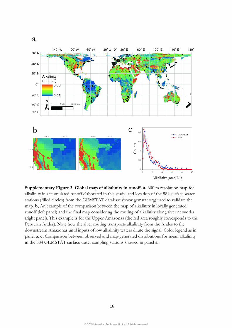
Supplementary Figure 3. Global map of alkalinity in runoff. a, 300 m resolution map for alkalinity in accumulated runoff elaborated in this study, and location of the 584 surface water stations (filled circles) from the GEMSTAT database (www.gemstat.org) used to validate the map. b, An example of the comparison between the map of alkalinity in locally generated runoff (left panel) and the final map considering the routing of alkalinity along river networks (right panel). This example is for the Upper Amazonas (the red area roughly corresponds to the Peruvian Andes). Note how the river routing transports alkalinity from the Andes to the downstream Amazonas until inputs of low alkalinity waters dilute the signal. Color legend as in panel a. c, Comparison between observed and map-generated distributions for mean alkalinity in the 584 GEMSTAT surface water sampling stations showed in panel a.





Supplementary Table 1. Chemical characteristics of the surface layer of the reservoirs

considered in this study. Data are detailed for both winter 1987 and summer 1988 sampling

campaigns, and include Age (years since first filling in 1987), trophic state indicators

(chlorophyll-a (Chl-a) and total phosphorus (TP) concentrations) and measurements of DO,

alkalinity, and partial pressure of dissolved CO2 (pCO2).

Summer

Winter

Moments and quantiles

Age (years)

Chl-a (µg L

-1)

TP (µmol L

-1)

DO (mmol L

-1)

Alkalinity (meq L

-1)

pCO2 (ppmv)

Chl-a (µg L

-1)

TP (µmol L

-1)

DO (mmol L

-1)

Alkalinity (meq L

-1)

pCO2 (ppmv)

Average 33 12.0 1.6 0.28 1.59 483

5.5 2.0 0.30 1.77 1235

Minimum 13 0.1 0.1 0.10 0.07 1

0.0 0.02 0.15 0.06 192

25% quartile 20 1.6 0.5 0.25 0.48 96

0.9 0.7 0.27 0.48 762

Median 27 3.9 0.7 0.28 1.64 378

1.9 1.2 0.29 1.68 1143

75% quartile 38 12.3 1.6 0.31 2.43 763

3.8 2.6 0.32 2.99 1532

Maximum 104 178.1 20.0 0.49 3.90 1939

215.4 20.2 0.48 4.69 3529





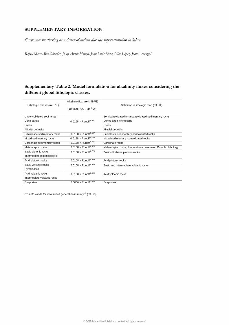
Supplementary Table 2. Model formulation for alkalinity fluxes considering the

different global lithologic classes.

Lithologic classes (ref. 51)

Alkalinity flux* (refs 49,51)

(106 mol HCO3

- km

-2 yr

-1)

Definition in lithologic map (ref. 52)

Unconsolidated sediments

0.0158 × Runoff 0.447

Semiconsolidated or unconsolidated sedimentary rocks

Dune sands Dunes and shifting sand

Loess Loess

Alluvial deposits Alluvial deposits

Siliciclastic sedimentary rocks 0.0158 × Runoff 0.537

Siliciclastic sedimentary consolidated rocks

Mixed sedimentary rocks 0.0158 × Runoff 0.734

Mixed sedimentary consolidated rocks

Carbonate sedimentary rocks 0.0158 × Runoff 0.746

Carbonate rocks

Metamorphic rocks 0.0158 × Runoff 0.324

Metamorphic rocks, Precambrian basement, Complex lithology

Basic plutonic rocks 0.0158 × Runoff 0.724

Basic-ultrabasic plutonic rocks

Intermediate plutonic rocks

Acid plutonic rocks 0.0158 × Runoff 0.449

Acid plutonic rocks

Basic volcanic rocks 0.0158 × Runoff 0.483

Basic and intermediate volcanic rocks

Pyroclastics

Acid volcanic rocks 0.0158 × Runoff 0.520

Acid volcanic rocks

Intermediate volcanic rocks

Evaporites 0.0006 × Runoff 1.000

Evaporites

*Runoff stands for local runoff generation in mm yr-1

(ref. 53)


Documents

Nature Research - Carbonate weathering as a driver …...Carbonate weathering as a driver of carbon dioxide supersaturation in lakes Rafael Marcé, Biel Obrador, Josep-Anton Morguí,