Embed Size (px)
Citation preview
nF nn
NAVAL POSTGRADUATE SCHOOL00Ln Monterey, California
0
TIIESISA COLUMN GENERATION TECHNIQUE FOR ACRISIS DEPLOYMENT PLANNING PROBLEM
by
Newton Rodrigues Lima
September 1988
Thesis Advisor: Siriphong Lawphongpanich
approved for public release; distribution is unlimited
DTICELECTE
E q 91988H
88 12 28 I091
UnclassifiedSECURITY CLASSIFICATION OF THIS PAGE
REPORT DOCUMENTATION PAGEI& REPORT SECURITY CLASSIFCATION lb RESTRICTIVE MARKINGSJnclassif ied
2. SECURITY CLASSIFICATION AUTHORITY 3 DISTRIBUTION/AVAILABILITY OF REPORTApproved for public release;
2b. DECLASSIFICATION /DOWNGRADING SCHEDULE Distribution is unlimited
4. PERFORMING ORGANIZATION REPORT NUMBER(S) S MONITORING ORGANIZATION REPORT NUMBER(S)
6& NAME OF PERFORMING ORGANIZATION 6b OFFICE SYMBOL 7a NAME OF MONITORING ORGANIZATION(If applicable)
Naval Postgraduate Schoolj 55 Naval Postgraduate School6c. ADDRESS (City, State. and ZIP Code) 7b ADDRESS (City. State. and ZIP Code)
Monterey, California 93943-5000 Monterey, California 93943-5000. NAME OF FUNDING, SPONSORING Sb OFFICE SYMBOL 9. PROCUREMENT INSTRUMENT IDENTIFICATION NUMBER
ORGANIZATION (If applicable)
k. ADDRESS (City, State, and ZIP Code) 10 SOURCE OF FUNDING NUMBERSPROGRAM PROJECT TASK WORK UNITELEMENT NO NO NO ACCESSION NO.
11 TITLE (Include Security Classification)A COLUMN GENERATION TECHNIQUE FOR A CRISIS DEPLOYMENT PLANNING PROBLEM
12 PERSONAL AUTHOR(S) LIMA, Newton Rodrigues13a TYPE OF REPORT I3b 'ME COVERED 14 DATE OF REPORT (Year, Month, Day) 15 PAGE COUNT
Master's Thesis FRONI! TO 1988 September I 416 SUPPLEMENTARY NOTATIONThe views expressed in this thesis are those of the authorand do not reflect the official policy or position of the Department ofDefense or th,- I -q r~nvyganm nyn-
17 COSATI CODES 18 SUBJl CT TERMS (Continue on reverse if necessary and identify b' block number)FIELD GROUP SUB-GROLP Dantzig-Wolte Decomoosition Method, Linear
Programming Optimization
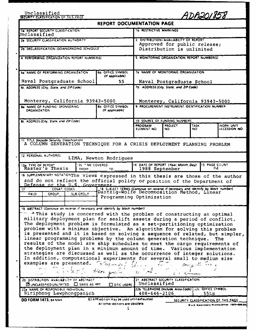
19 ABSTRACT (Continue on reverse if necessary and identify by block number)
..... -This study is concerned with the problem of constructing an optimalmilitary deployment plan for sealift assets during a period of conflict.The deployment problem is formulated as a set-partitioning optimizationproblem with a minimax objective. An algorithm for solving this problemis presented and it is based on solving a sequence of related, but simpler,linear programming problems by the column generation technique. Theresults of the model are ship schedules to meet the cargo requirements ofthe deployment plan in a minimum amount of time. Various implementationstrategies are discussed as well as the occurrence of integer solutions.In addition, computational experiments for several small to medium sizeexamples are presented. .. ,' ' - -
.. .f ! .- , "k. •" i-
20 DISTRIBUTION AVAIL4UILITY Of A0STRACT 21 ABSTRACT SECURITY CLASSIFICATION
MUNCLASSIFIED/UNLIMITED 0 SAM.E AS RPT 0 DTIC USERS Unclassified22a NAME OF RESPONSIBLE INDIVIDUAL 22b TELEPHONE (Include Area Code) j2c OFFICE SYMBOL
Siriphong Lawphongpanich 408-646-2106 I 55LpDD FORM 1473, 84 MAR 83 APR edition may be used until exhausted SECURITY CLASSIFICATION OF THIS PAGE
All other editions are obsolete * . Qov,, fl , o . -i
Approved for public release; distribution is unlimited.
A Column Generation Technique For ACrisis Deployment Planning Problem
by
Newton Rodrigues LimaLieutenant, Brazilian Navy
B.S., Escola Naval, Rio de Janeiro, Brazil, 1977
Submitted in partial fulfillment of therequirements for the degree of
MASTER OF SCIENCE IN OPERATIONS RESEARCH
from the
NAVAL POSTGRADUATE SCHOOLSeptember 1988
Author:Ne YNewtbn Rodrigues LimaU
Approved by:Siriphon fLawphbngpahich, Thesis Advisor
Richard E. Rosenthal, Second Reader
Peter Pxfrdue, Chairman, Departmentof Operations Research
gneale T. MiitDean of Information and Poi-i Sciences
ABSTRACT
This study is concerned with the problem of
constructing an optimal military deployment plan for
sealift assets during a period of conflict. The deployment
problem is formulated as a set-partitioning optimization
problem with a minimax objective. An algorithm for solving
this problem is presented and it is based on solving a
sequence of related, but simpler, linear programming
problems by the column generation technique. The results
of the model are ship schedules to meet the cargo
requirements of the deployment plan in a minimum amount of
time. Various implementation strategies are discussed as
well as the occurrence of integer solutions. In addition,
computational experiments for several small to medium size
examples are presented.
Acoession For
NTIS GRA&IDTIC TAB QUnan-notmeed 0]
By~.Just ifbict "on---
Availability Codes
Dist Specialii AKib'/
TABLE OF CONTENTS
I. INTRODUCTION ......................................... 1
A. PROBLEM STATEMENT ................................ 1
B. BACKGROUND ....................................... 2
C. OBJECTIVE ........................................ 3
II. PROBLEM FORMULATION .................................. 4
A. MATHEMATICAL FORMULATION ......................... 4
B. AN EXAMPLE ....................................... 7
III. A SEQUENTIAL SOLUTION TECHNIQUE ...................... 12
A. A RELATED PROBLEM ............................... 12
B. A COLUMN GENERATION APPROACH TO THE
FEASIBILITY-SEEKING PROBLEM ...................... 14
IV. IMPLEMENTATION AND COMPUTATIONAL RESULTS ............ 20
A. PROBLEM DATA .................................... 20
B. STRATEGIES FOR GENERATING SCHEDULES ............. 24
C. SOLVING THE MINIMAX PROBLEM ...................... 25
D. PERCENTAGE OF INTEGER SOLUTIONS ................. 33
V. CONCLUSIONS AND FUTURE STUDIES ....................... 34
APPENDIX FORTRAN PROGRAM ............................ 36
LIST OF REFERENCES .................................. 76
INITIAL DISTRIBUTION LIST ........................... 77
iv

ACKNOWLEDGEMENTS
I wish to dedicate this thesis to my wifeli and
mywchildren for all their loving
support and continuing encouragement throughout this
lcngthy journey. Without their assistance, this project
could not have been undertaken.
To my thesis advisor, Professor Siriphong
Lawphongpanich, I would like to thank for his sound advice,
technical guidance and editorial assistance.
F-..nally,, I am especially grateful to my friends LT
Carlos Vallejo (Ecuadorian Navy), CPT Edward Koucheravy
(U.S. Army) and LCDR Svein Buvik (Norwegian Navy) for all
their aid, critique and moral support throughout this
study.
V
I. INTRODUCTION
A. PROBLEM STATEMENT
During a military deployment, troops, equipments and
supplies must be transported from ports of embarkation to
ports of disembarkation. Generally, the standard modes of
transportation used in this operation are trucks, trains,
airplanes and ships. Because of the limited amount of
available resources and transport assets, planning becomes
essential for a successful deployment. During peacetime,
cargo transportation can be routinely scheduled and the
normal criterion for a deployment plan is its cost (or
operating expense). However, during a period of conflict
(or crisis), expenses become secondary and it is more
important to transport the troops and cargoes to their
destinations as fast as possible.
This study restricts itself to the problem of
constructing an optimal deployment plan which employs only
sealift assets. Many of today's naval deployment plans are
constructed manually and in an ad hoc manner. This process
is quite time-consuming and does not guarantee to produce
even a near optimal plan.
• . • m m ! l l1
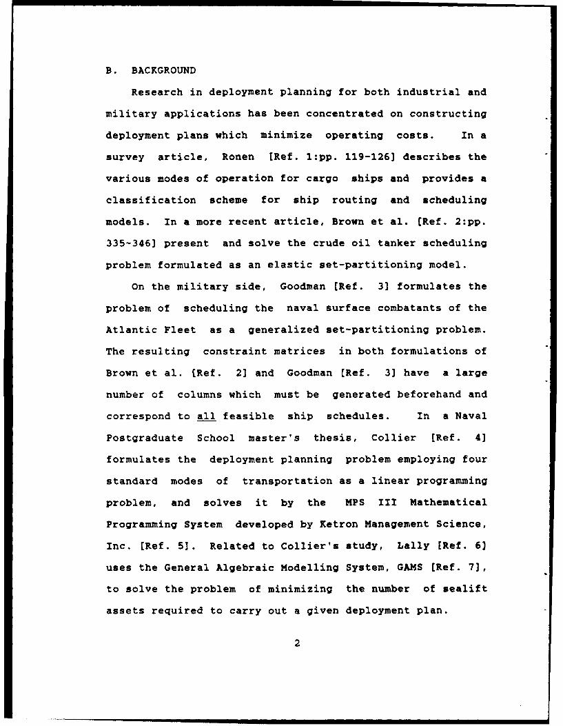
B. BACKGROUND
Research in deployment planning for both industrial and
military applications has been concentrated on constructing
deployment plans which minimize operating costs. In a
survey article, Ronen [Ref. 1:pp. 119-126] describes the
various modes of operation for cargo ships and provides a
classification scheme for ship routing and scheduling
models. In a more recent article, Brown et al. [Ref. 2:pp.
335-346] present and solve the crude oil tanker scheduling
problem formulated as an elastic set-partitioning model.
On the military side, Goodman [Ref. 3] formulates the
problem of scheduling the naval surface combatants of the
Atlantic Fleet as a generalized set-partitioning problem.
The resulting constraint matrices in both formulations of
Brown et al. [Ref. 2] and Goodman [Ref. 3] have a large
number of columns which must be generated beforehand and
correspond to all feasible ship schedules. In a Naval
Postgraduate School master's thesis, Collier [Ref. 4]
formulates the deployment planning problem employing four
standard modes of transportation as a linear programming
problem, and solves it by the MPS III Mathematical
Programming System developed by Ketron Management Science,
Inc. [Ref. 5]. Related to Collier's study, Lally [Ref. 6]
uses the General Algebraic Modelling System, GAMS [Ref. 7],
to solve the problem of minimizing the number of sealift
assets required to carry out a given deployment plan.
2
C. OBJECTIVE
In previous formulations of the deployment or ship
scheduling problem, the primary objective is to minimize
cost which is the most appropriate for peace-time military
operations and for industry. This thesis addresses the
same problem, but with a different objective: to minimize
the duration of the deployment. In particular, it
considers the construction of schedules for sealift assets
to transport cargoes from their ports of origin to their
ports of destination in the minimum length of time.
3
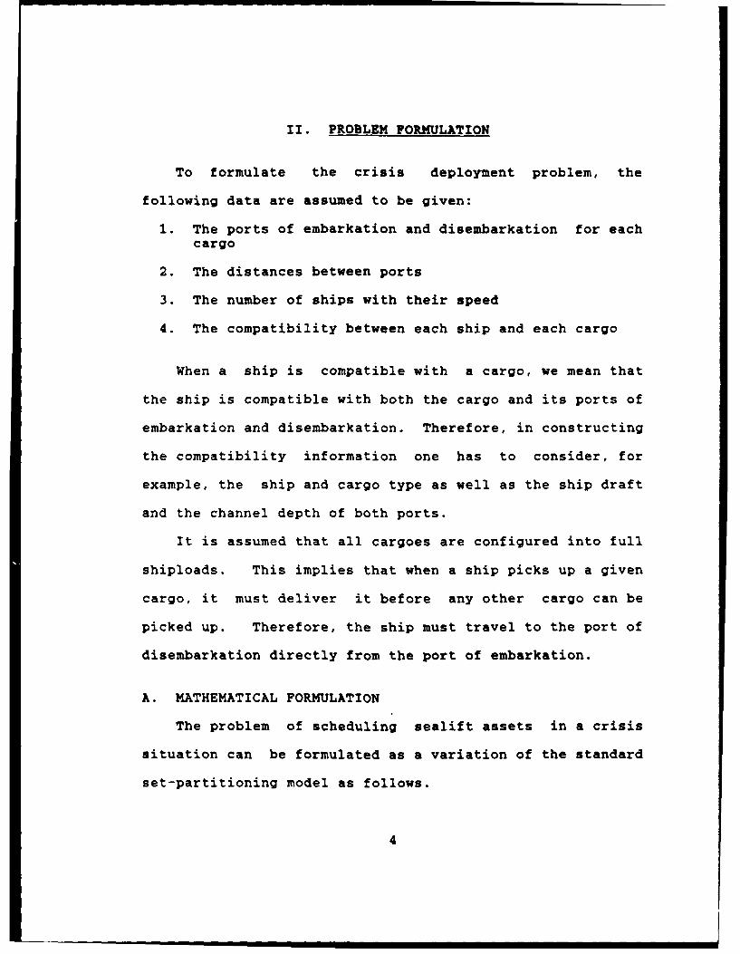
II. PROBLEM FORMULATION
To formulate the crisis deployment problem, the
following data are assumed to be given:
1. The ports of embarkation and disembarkation for eachcargo
2. The distances between ports
3. The number of ships with their speed
4. The compatibility between each ship and each cargo
When a ship is compatible with a cargo, we mean that
the ship is compatible with both the cargo and its ports of
embarkation and disembarkation. Therefore, in constructing
the compatibility information one has to consider, for
example, the ship and cargo type as well as the ship draft
and the channel depth of both ports.
It is assumed that all cargoes are configured into full
shiploads. This implies that when a ship picks up a given
cargo, it must deliver it before any other cargo can be
picked up. Therefore, the ship must travel to the port of
disembarkation directly from the port of embarkation.
A. MATHEMATICAL FORMULATION
The problem of scheduling sealift assets in a crisis
situation can be formulated as a variation of the standard
set-partitioning model as follows.
4
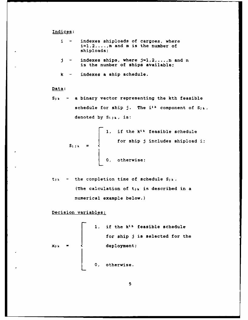
Indices:
i - indexes shiploads of cargoes, wherei=1,2,...,m and m is the number ofshiploads;
j - indexes ships, where j=1,2,...,n and nis the number of ships available;
k - indexes a ship schedule.
Data:
SJ - a binary vector representing the kth feasible
schedule for ship j. The it h component of Sik,
denoted by SIjk, is:
F 1, if the kth feasible schedule
for ship j includes shipload i;St Jk= <
L 0, otherwise;
tJk the completion time of schedule Sjk.
(The calculation of tJk is described in a
numerical example below.)
Decision variables:
1, if the ktb feasible schedule
for ship j is selected for the
xjk = < deployment;
0, otherwise.
5
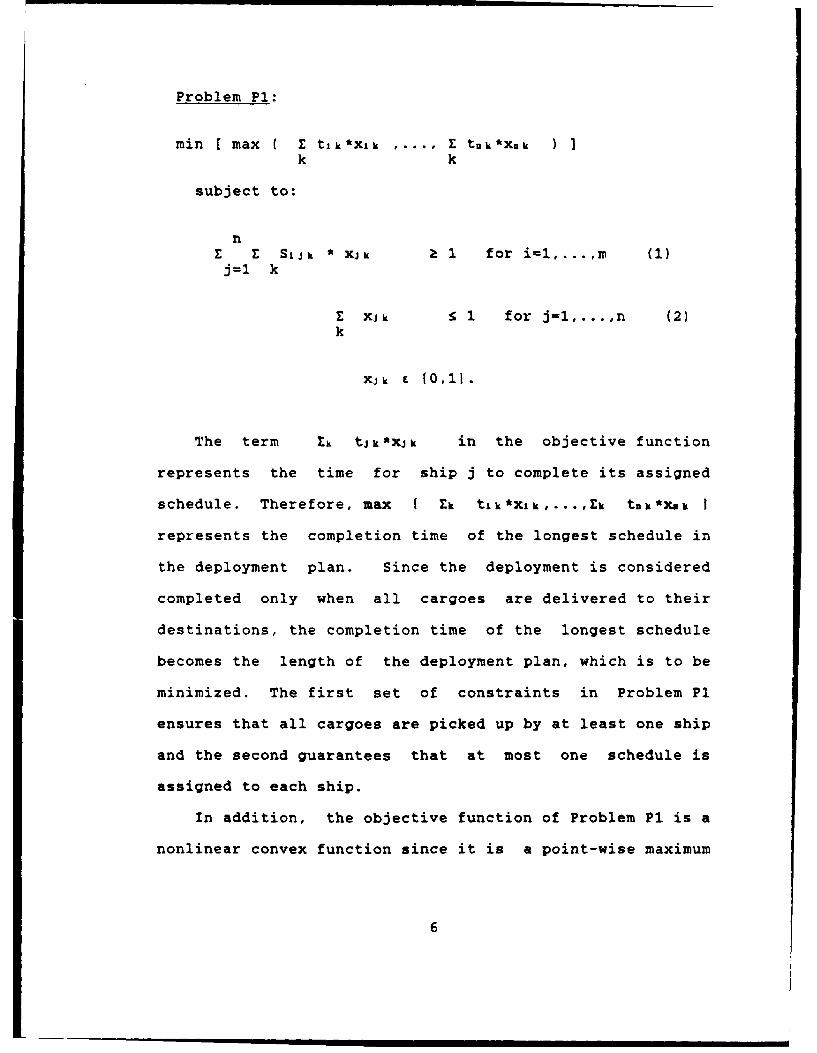
Problem P1:
min [ max I E tlk*Xlk E.... E tnk*Xk )k k
subject to:
nE E SIJk * XJk 1 for i=l ....m (1)j=1 k
Z XJk 5 1 for j=1,...,n (2)k
Xjk E 10,11.
The term Z tjk*xjk in the objective function
represents the time for ship j to complete its assigned
schedule. Therefore, max E Ek tlk*Xlk,...,Ek tnk*Xak I
represents the completion time of the longest schedule in
the deployment plan. Since the deployment is considered
completed only when all cargoes are delivered to their
destinations, the completion time of the longest schedule
becomes the length of the deployment plan, which is to be
minimized. The first set of constraints in Problem P1
ensures that all cargoes are picked up by at least one ship
and the second guarantees that at most one schedule is
assigned to each ship.
In addition, the objective function of Problem P1 is a
nonlinear convex function since it is a point-wise maximum
6
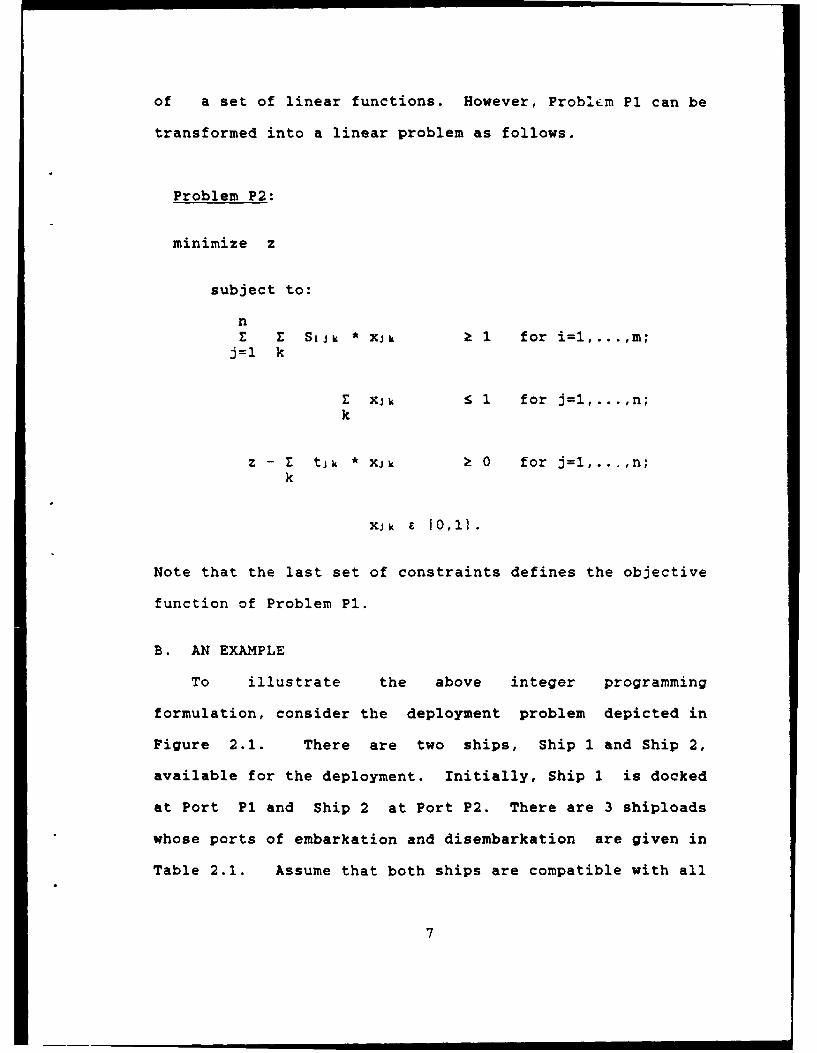
of a set of linear functions. However, Problem P1 can be
transformed into a linear problem as follows.
Problem P2:
minimize z
subject to:
nr Z SiJk * XJk 1 for i=l ....m;
j=l k
E XJk 1 for j=l,...,n;k
z - E tik * XJk 2 0 for j=l,...,n;k
xjk E 0, }.
Note that the last set of constraints defines the objective
function of Problem P1.
B. AN EXAMPLE
To illustrate the above integer programming
formulation, consider the deployment problem depicted in
Figure 2.1. There are two ships, Ship 1 and Ship 2,
available for the deployment. Initially, Ship 1 is docked
at Port P1 and Ship 2 at Port P2. There are 3 shiploads
whose ports of embarkation and disembarkation are given in
Table 2.1. Assume that both ships are compatible with all
7
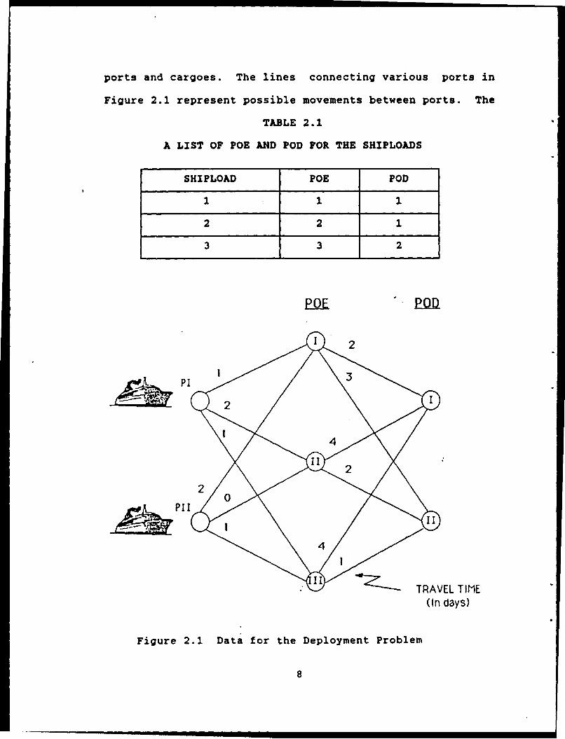
ports and cargoes. The lines connecting various ports in
Figure 2.1 represent possible movements between ports. The
TABLE 2.1
A LIST OF POE AND POD FOR THE SHIPLOADS
SHIPLOAD POE POD
1 1 1
2 2 1
3 3 2
2
PI 2
(In days)
Figure 2.1 Data for the Deployment Problem
.4
numbers adjacent to the lines represent the travel times
for both ships, i.e., they have the same speed (assumed
constant regardless of cargo loading).
Consider a schedule for Ship 1 which includes picking
up cargoes 1 and 3. The binary vector representing this
schedule has 3 components (since there are 3 shiploads)
with the first and the third components having the value
one and the second component the value zero. To carry out
this schedule, Ship 1 can use one of the two possible
routes: one which picks up cargo 1 first and then cargo 3
and the other which picks up the cargoes in the reverse
order. Using the time given in Figure 2.1, the first route
requires 8 days to complete and the second requires only 7
days. Since the objective is to minimize the completion
time of the longest schedule, the completion time of 7 days
is assigned to this schedule, i.e., t,4 = 7. In general,
the completion time tjk is the time for ship j to carry out
schedule k using the shortest route. Tables 2.2 and 2.3
display all possible schedules along with their completion
times for Ships 1 and 2, respectively. Note that the
schedule discussed above is the schedule S,4 in Table 2.2.
The optimal deployment plan for this example consists
of two schedules: Siz for Ship 1 and S24 for Ship 2, and
requires 7 days to complete. In terms of decision
variables, X12 and X24 equal one and all other variables
equal zero.
9
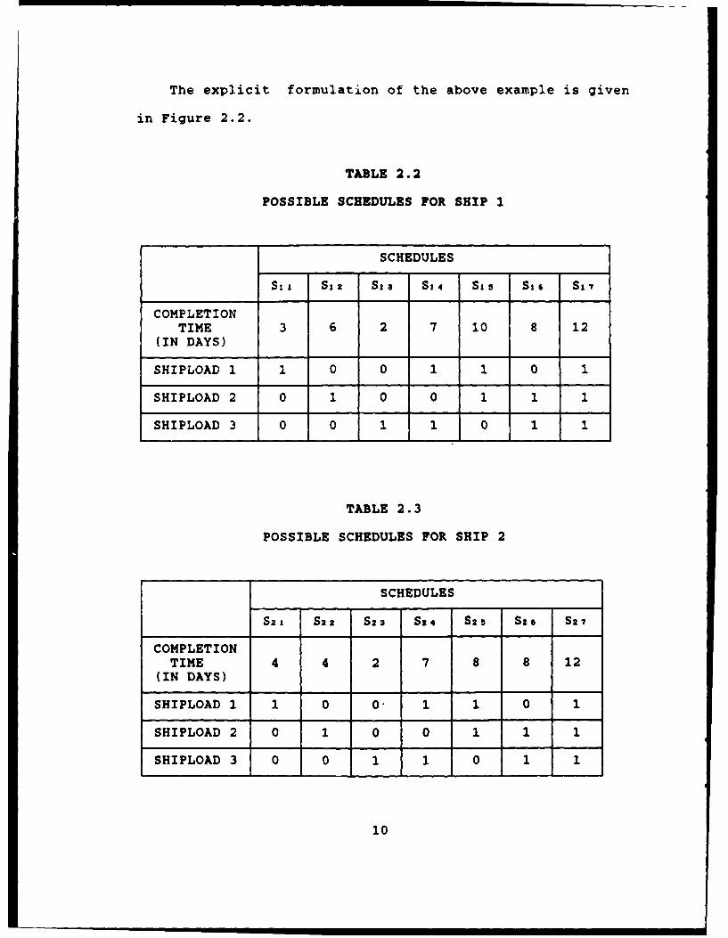
The explicit formulation of the above example is given
in Figure 2.2.
TABLE 2.2
POSSIBLE SCHEDULES FOR SHIP 1
SCHEDULES
Sit Si2 S1a S14 Sis Si. SIT
COMPLETIONTIME 3 6 2 7 10 8 12
(IN DAYS)
SHIPLOAD 1 1 0 0 1 1 0 1
SHIPLOAD 2 0 1 0 0 1 1 1
SHIPLOAD 3 0 0 1 1 0 1
TABLE 2.3
POSSIBLE SCHEDULES FOR SHIP 2
SCHEDULES
S21 S22 S23 S24 S25 S2, Sz7
COMPLETIONTIME 4 4 2 7 8 8 12
(IN DAYS)
SHIPLOAD 1 1 0 0. 1 1 0 1
SHIPLOAD 2 0 1 0 0 1 1 1
SHIPLOAD 3 0 0 1 1 0 1 1
10
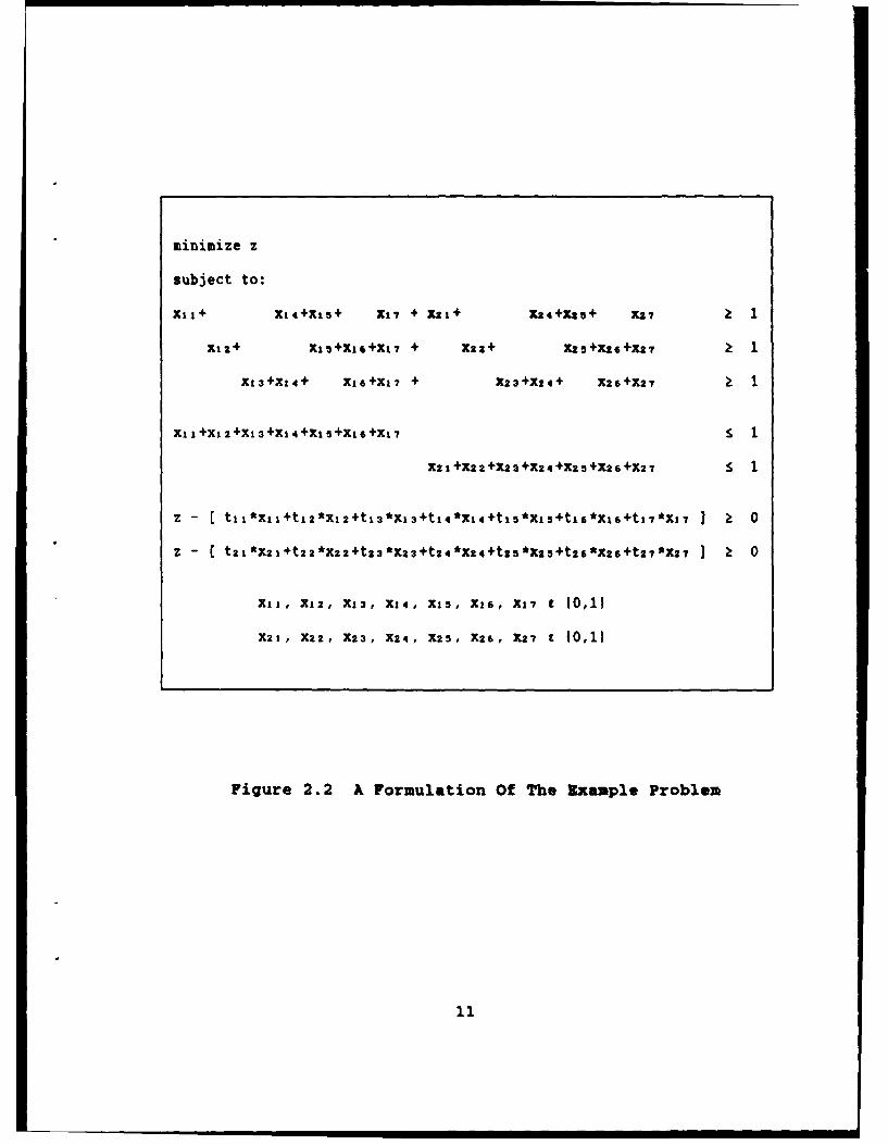
minimize z
subject to:
X11+ X14+XIS+ X17 + Ku14 X24+X25+ X27 1
X12+ Xifl+XuI+XiI + X22+ X2 5 X2 G+X2 7
X13+X14+ X16+XI? + X23+X241+ X2B+X27 1
Xli +XIZ+X13+X14+Xl5+XI6+X17S1
X21+XZ2+X2a+X24+X25+X26+X27 S 1
Z - [tll*XII+t12*Xi2+tl3*Xl3+tl4*Xi4+tl5*Xl5+tlG*XlS+tl7*XI7 k 0
Z - (t21*X21+t22*X22+t23*X23+t24*X24+t25*X25+t26*X26+t27*X2? k 0
XII, X12, X13, X14, X15, X16, XI? t 10,11
X21, X22, X23, X24, X25, X26, X27 E 10,11
Figure 2.2 A Formulation Of The Example Problem
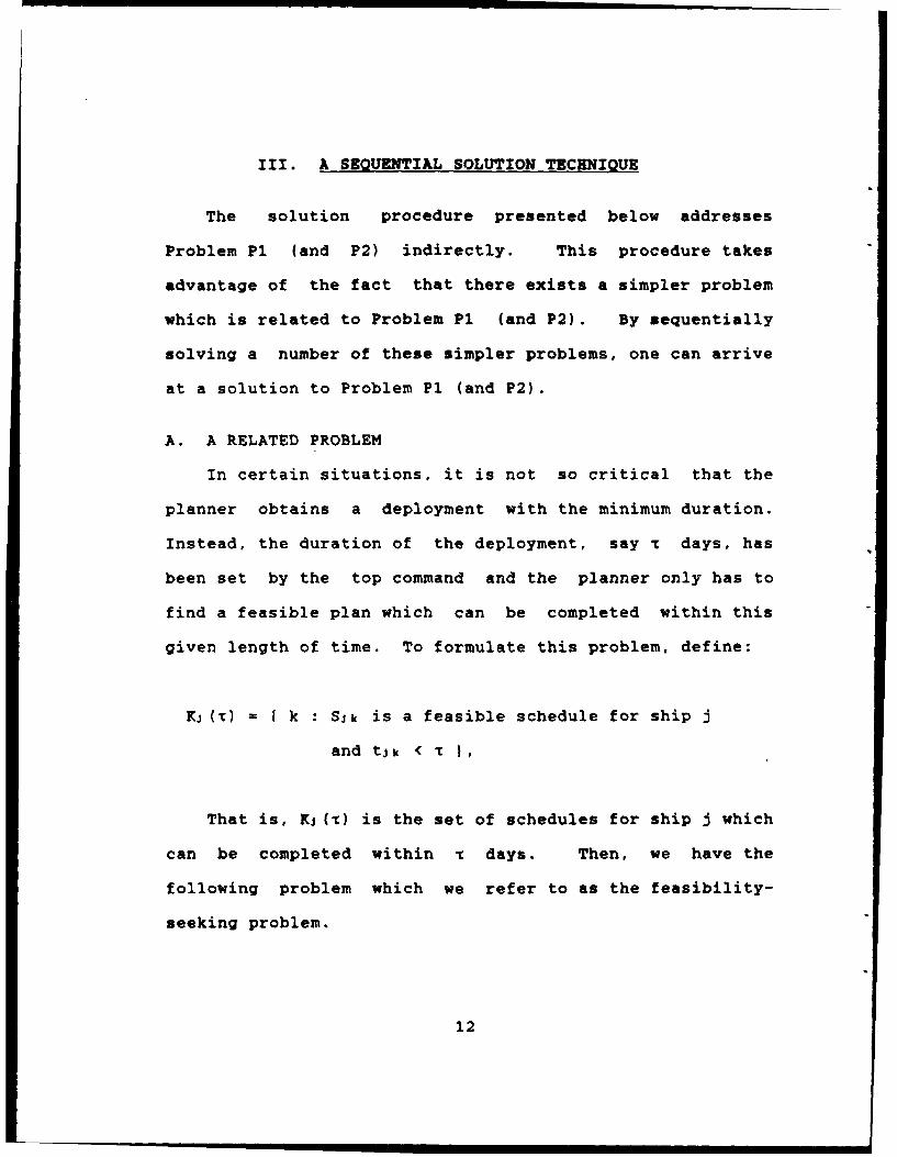
III. A SEQUENTIAL SOLUTION TECHNIQUE
The solution procedure presented below addresses
Problem P1 (and P2) indirectly. This procedure takes
advantage of the fact that there exists a simpler problem
which is related to Problem P1 (and P2). By sequentially
solving a number of these simpler problems, one can arrive
at a solution to Problem P1 (and P2).
A. A RELATED PROBLEM
In certain situations, it is not so critical that the
planner obtains a deployment with the minimum duration.
Instead, the duration of the deployment, say T days, has
been set by the top command and the planner only has to
find a feasible plan which can be completed within this
given length of time. To formulate this problem, define:
Kj (t) = k : SJk is a feasible schedule for ship j
and tj k < T ,
That is, Kj (,r) is the set of schedules for ship j which
can be completed within % days. Then, we have the
following problem which we refer to as the feasibility-
seeking problem.
12
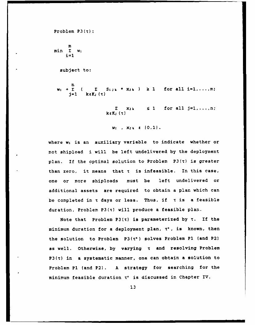
Problem P3(t):
mmin Z wi
i=l
subject to:
nWI + E ( E SIJk * XJk ) 1 for all i=l....m;
j=1 kEKj (,)
E xJk 1 for all j=l,...,n;
W1 , xjk 10,11.
where wi is an auxiliary variable to indicate whether or
not shipload i will be left undelivered by the deployment
plan. If the optimal solution to Problem P3(T) is greater
than zero, it means that T is infeasible. In this case,
one or more shiploads must be left undelivered or
additional assets are required to obtain a plan which can
be completed in T days or less. Thus, if T is a feasible
duration, Problem P3(x) will produce a feasible plan.
Note that Problem P3(t) is parameterized by T. If the
minimum duration for a deployment plan, T*, is known, then
the solution to Problem P3( *) solves Problem P1 (and P2)
as well. Otherwise, by varying x and resolving Problem
P3(t) in a systematic manner, one can obtain a solution to
Problem P1 (and P2). A strategy for searching for the
minimum feasible duration T* is discussed in Chapter IV.
13
To illustrate the feasibility-seeking problem, consider
the deployment problem presented in Chapter II. Assume
that the planner is told to construct a plan with a
duration of 8 days.
Then,
K,(8) = 1 1, 2, 3, 4, 6 1 and
Kz(8) = 1 1, 2, 3, 4, 5, 6 1,
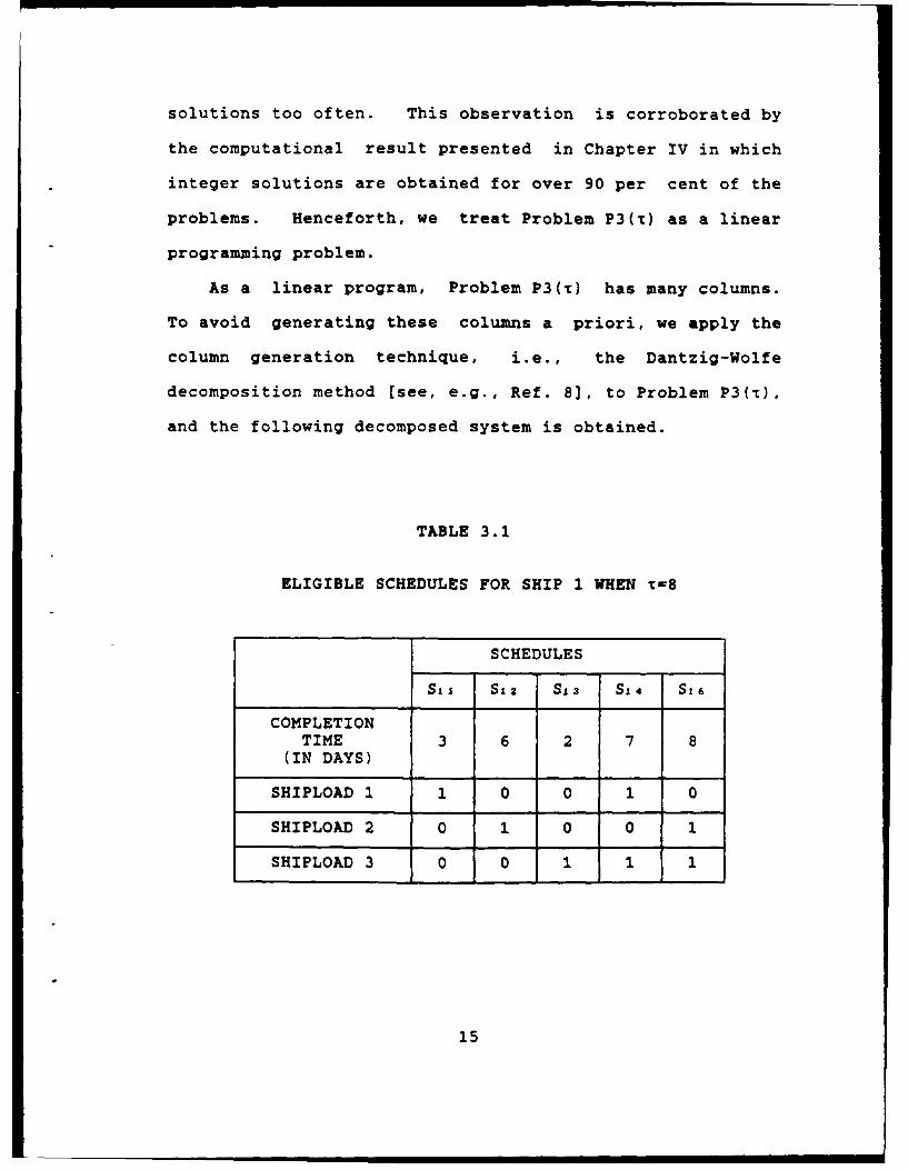
that is, the eligible schedules for this plan with a
completion time of 8 days or less are those listed Tables
3.1 and 3.2. In this case, the optimal objective function
value for Problem P3(8) is zero, because 8 days is a
feasible duration. Each of the following pairs of
schedules for Ships 1 and 2: (Si,S2), (S12,S24 ),
(S13,S25), (S14,S22), and (S 6,S21), constitutes a
deployment plan that can be completed within 8 days.
Similarly, if one solves Problem P3(t) with T equal to
7 days (the optimal duration), the optimal objective
function value is still zero, and the pairs (Siz,Sz4) and
(S14 ,S22) are the only feasible deployment plans.
B. A COLUMN GENERATION APPROACH TO THE FEASIBILITY-SEEKING
PROBLEM
Since the feasibility-seeking problem searches for a
feasible deployment plan and does not have a real objective
function to optimize, one expects that the relaxation of
the integrality restriction would not produce fractional
14
solutions too often. This observation is corroborated by
the computational result presented in Chapter IV in which
integer solutions are obtained for over 90 per cent of the
problems. Henceforth, we treat Problem P3(x) as a linear
programming problem.
As a linear program, Problem P3(r) has many columns.
To avoid generating these columns a priori, we apply the
column generation technique, i.e., the Dantzig-Wolfe
decomposition method [see, e.g., Ref. 8], to Problem P3(T),
and the following decomposed system is obtained.
TABLE 3.1
ELIGIBLE SCHEDULES FOR SHIP 1 WHEN T-8
SCHEDULES
S11 S1z S13 S14 S16
COMPLETIONTIME 3 6 2 7 8
(IN DAYS)
SHIPLOAD 1 1 0 0 1 0
SHIPLOAD 2 0 1 0 0 1
SHIPLOAD 3 0 0 1 1 1
15
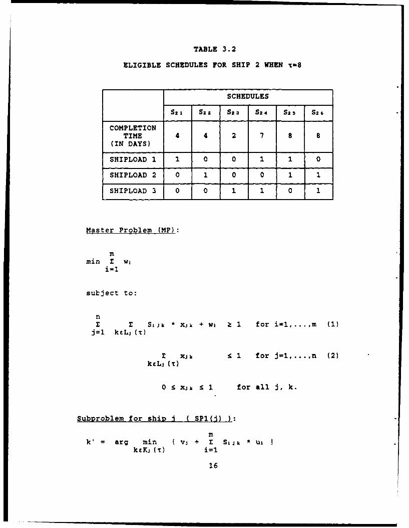
TABLE 3.2
ELIGIBLE SCHEDULES FOR SHIP 2 WHEN x-8
SCHEDULES
S21 S2z S23 S24 S.s- S26
COMPLETIONTIME 4 4 2 7 8 8
(IN DAYS)
SHIPLOAD 1 1 0 0 1 1 0
SHIPLOAD 2 0 1 0 0 1 1
SHIPLOAD 3 0 0 1 1 0 1
Master Problem (MP):
mm Inmnin X wii=1
subject to:
nE z SAJk * XJk + wi k 1 for i=l.... (1)j=1 ktLj (-)
E XJk 1 for j=l,...,n (2)k cLj (-)
0 < xJh S 1 for all j, k.
Subproblem for ship ( SP1(j) ):
mk'= arg min I Vj + t S1Jk * U1
ktKi (-r) i=l
16
where ut is the dual variable corresponding to constraint
set (1), i.e., the cargo (shipload) constraints, and vj is
the dual variable corresponding to the constraint set (2),
i.e., the ship constraints. We refer to ul as the ith
cargo dual and vj as the jtb ship dual.
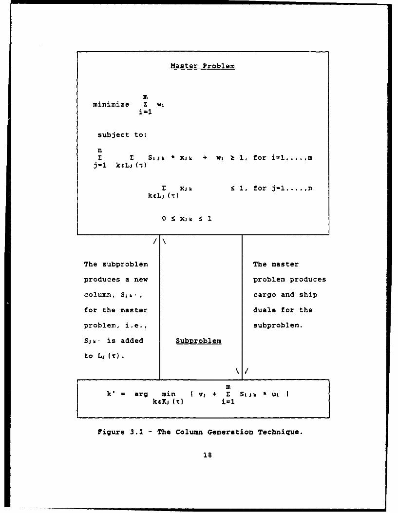
The column generation technique starts with an initial
set of feasible schedules, Li ( ), for each ship j. This
initial set Lj () may be an empty set. The master problem
is solved and the dual variables ui and vj are obtained.
From this set of cargo and ship duals, one or more
subproblems are solved thereby generating additional
schedules (columns), Sjk', which are subsequently added to
the set Lj (t). The master problem is then resolved with
the additional schedules (columns) and the new cargo and
ship duals are obtained. The cycle then continues until
the objective function value of Problem SP(j) is
nonnegative for all j, i.e., all schedules have nonnegative
reduced cost. This signifies that optimality is achieved.
Figure 3.1 illustrates the cycling between the master and
subproblem in the column generation technique.
As stated above, the subproblem is unnecessarily hard.
In theory, it is not necessary to add schedules (columns)
with the most negative reduced cost to the master problem.
Any schedules (columns) with negative reduced cost would
suffice. The following subproblem produces negative
reduced cost schedules for the master problem.
17
Master Problem
mminimize Z w1
i=1
subject to:
nZ E SiJk * XJik + Wi k 1, for i=1....m
j=l kEL (-)
E xJk S 1, for j=l,...nkELj (x )
0 S XJk 1
The subproblem The master
produces a new problem produces
column, SJk' , cargo and ship
for the master duals for the
problem, i.e., subproblem.
Sjik. is added SubDroblem
to Li ().
mk'= arg min I Vj + E SIJk * U
ktKj (t) i=1
Figure 3.1 - The Column Generation Technique.
18
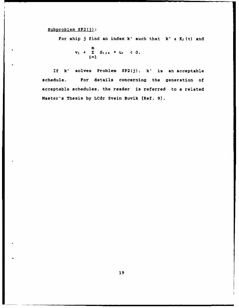
Subproblem SP2(j):
For ship j find an index k' such that k' z Kj (x) and
mvj + Z SiJk * ul <0.i=1
If k' solves Problem SP2(j), k' is an acceptable
schedule. For details concerning the generation of
acceptable schedules, the reader is referred to a related
Master's Thesis by LCdr Svein Buvik [Ref. 9].
19
IV. IMPLEMENTATION AND COMPUTATIONAL RESULTS
To implement the column generation procedure we
modified the revised simplex code described in Ref. 10, to
solve the master problem. In this modification, we allow
the algorithm to restart from the last optimal solution
after one or more new schedules (columns) have been added
to the master problem. Since the set partitioning problem
is usually degenerate, we also reinvert the basis at every
ten iterations. As for the subproblem, we employ the
algorithm developed by Buvik [Ref. 9]. Both the master and
subproblem algorithms are written in FORTRAN 77 and
compiled by the IBM VS FORTRAN compiler. All runs were
performed on an IBM 3033 AP computer at the W.R. Church
Computer Center of the Naval Postgraduate School.
A. PROBLEM DATA
For our experimentation below, we consider the
deployment scenario in which cargoes must be moved from the
ports along the east coast of United States to ports in
Europe. Table 4.1 lists approximate distances between
various ports. The number of shiploads for our deployment
problems are varied between 5 and 50 and the list of all 50
shiploads along with their POE's and POD's are given in
Table 4.2. The number of ships assigned to the deployment
are assumed to be between 2 and 30 ships and the initial
20
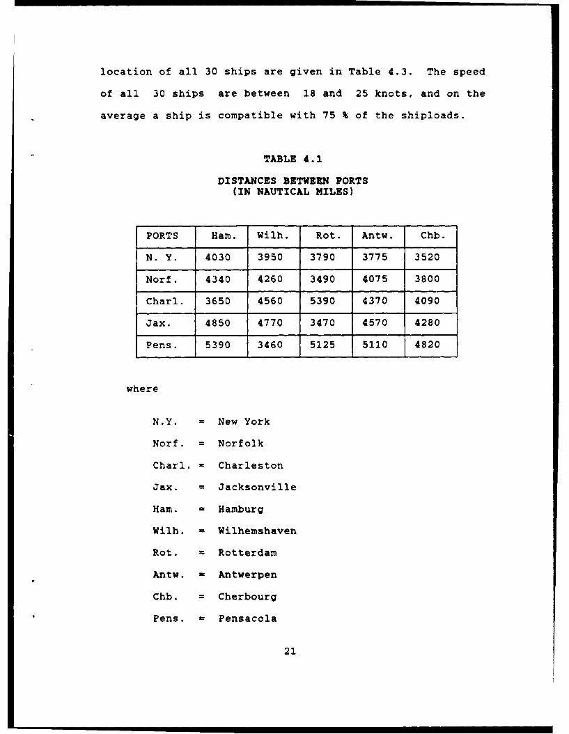
location of all 30 ships are given in Table 4.3. The speed
of all 30 ships are between 18 and 25 knots, and on the
average a ship is compatible with 75 % of the shiploads.
TABLE 4.1
DISTANCES BETWEEN PORTS(IN NAUTICAL MILES)
PORTS Ham. Wilh. Rot. Antw. Chb.
N. Y. 4030 3950 3790 3775 3520
Norf. 4340 4260 3490 4075 3800
Chari. 3650 4560 5390 4370 4090
Jax. 4850 4770 3470 4570 4280
Pens. 5390 3460 5125 5110 4820
where
N.Y. = New York
Norf. = Norfolk
Charl. = Charleston
Jax. = Jacksonville
Ham. = Hamburg
Wilh. = Wilhemshaven
Rot. = Rotterdam
Antw. Antwerpen
Chb. = Cherbourg
Pens. = Pensacola
21
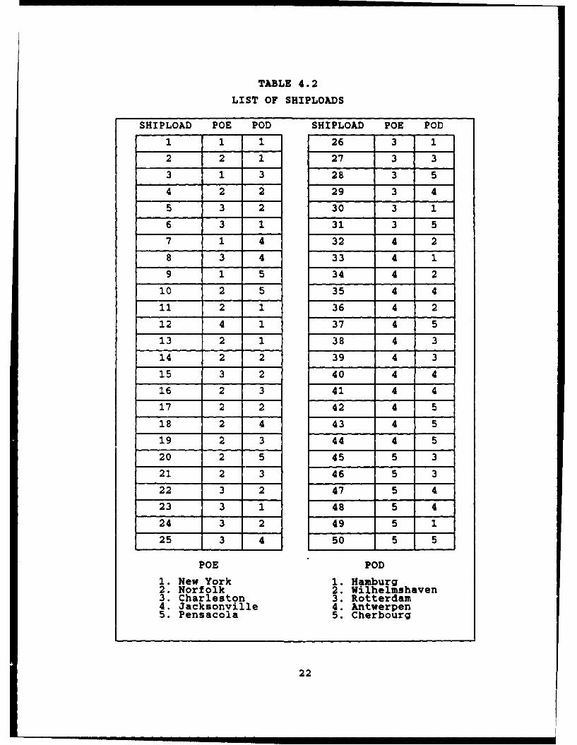
TABLE 4.2
LIST OF SHIPLOADS
SHIPLOAD POE POD SHIPLOAD POE POD
1 1 1 26 3 1
2 2 1 27 3 3
3 1 3 28 3 5
4 2 2 29 3 4
5 3 2 30 3 1
6 3 1 31 3 5
7 1 4 32 4 2
8 3 4 33 4 1
9 1 5 34 4 2
10 2 5 35 4 4
11 2 1 36 4 2
12 4 1 37 4 5
13 2 1 38 4 3
14 2 2 39 4 3
15 3 2 40 4 4
16 2 3 41 4 4
17 2 2 42 4 5
18 2 4 43 4 5
19 2 3 44 4 5
20 2 5 45 5 3
21 2 3 46 5 3
22 3 2 47 5 4
23 3 1 48 5 4
24 3 2 49 5 1
25 3 4 50 5 5
POE POD
1. New York 1. Hamburg2. Norfolk 2. Wilhelmshaven3. Charleston 3. Rotterdam4. Jacksonville 4 Antwerpen5. Pensacola 5. Cherbourg
22
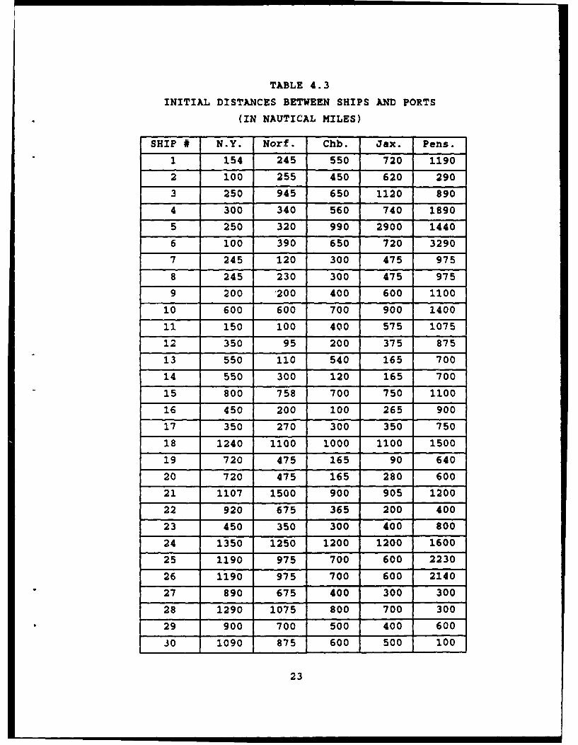
TABLE 4.3
INITIAL DISTANCES BETWEEN SHIPS AND PORTS
(IN NAUTICAL MILES)
SHIP # N.Y. Norf. Chb. Jax. Pens.
1 154 245 550 720 1190
2 100 255 450 620 290
3 250 945 650 1120 890
4 300 340 560 740 1890
5 250 320 990 2900 1440
6 100 390 650 720 3290
7 245 120 300 475 975
8 245 230 300 475 975
9 200 200 400 600 1100
10 600 600 700 900 1400
11 150 100 400 575 1075
12 350 95 200 375 875
13 550 110 540 165 700
14 550 300 120 165 700
15 800 758 700 750 1100
16 450 200 100 265 900
17 350 270 300 350 750
18 1240 1100 1000 1100 1500
19 720 475 165 90 640
20 720 475 165 280 600
21 1107 1500 900 905 1200
22 920 675 365 200 400
23 450 350 300 400 800
24 1350 1250 1200 1200 1600
25 1190 975 700 600 2230
26 1190 975 700 600 2140
27 890 675 400 300 300
28 1290 1075 800 700 300
29 900 700 500 400 600
30 1090 875 600 500 100
23
B. STRATEGIES FOR GENERATING SCHEDULES
As described in Chapter III, the decomposition process
iteratively solves the master and subproblem in sequence.
After having just solved the master problem, the subproblem
obtains the cargo and ship duals from which it generates
one or more negative reduced cost columns. At this point,
there are several possibilities regarding the ship(s) for
which the subproblem should generate schedules (or
columns). The first obvious strategy is to generate a
schedule for Ship 1 in the first iteration, a schedule of
Ship 2 in the second iteration and so on until a schedule
for each ship has been generated. At which point, the
cycle of generating schedules (columns) begins again with
Ship 1. The second strategy is to generate schedules for
ship in the descending order of the ship duals, and the
third strategy is just the reverse of the second strategy,
i.e., generates schedules in the ascending order of the
ship duals. The other strategy, which has been considered
and soon after discarded, generates schedules for all ships
during each iteration. This strategy tends to generate the
same schedule for all ships, which seems redundant since no
two ships can have the same schedule at optimality. In
fact, there must exists a solution in which no two ships
are assigned to pick up the same shipload. Based on this
observation and preliminary experiments, the last strategy
is discarded.
24
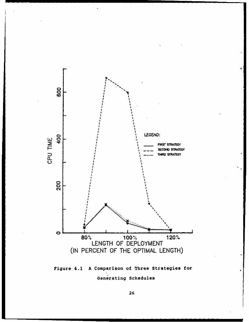
To compare the three strategies discussed above, we
solved three feasibility-seeking problems at various
lengths of deployment, x. The first problem has 30
shiploads and 20 ships, the second problem has 35 shiploads
and 20 ships, and the last has 40 shiploads and 20 ships.
In Figure 4.1, we plotted the average cpu times on these
three problems against the length of deployment. The first
and third strategies clearly dominate the second.
C. SOLVING THE MINIMAX PROBLEM
As mentioned in Chapter III, one can solve the minimax
problem by sequentially solving the feasibility-seeking
problem in the following manner. First, pick an initial
value for i and then solve the feasibility-seeking problem
at this value T. If the optimal objective function is
zero, then the value of x is decreased and the feasibility-
seeking problem is resolved at the new value. Otherwise,
the optimal objective function is positive, the value for T
is increased and the feasibility-seeking problem is
resolved.
The efficiency of the above algorithm is clearly a
function of the initial value for T. If the initial value
for x is close to the optimal, the feasibility-seeking
problem has to be solved less often. Thus, it is important
that a good initial value for T is used to start the
process of increasing and decreasing the value x.
25
0 % %,'N
o|
oJ 0SEON STATG
I I
I I
1 4
I I
Figure~~~~~~ 4.1S A opaio o heeSrtegeYo
------ SECOND STIEGYGenranTHIRD STRATEGY
o 2I II I
I II II II I
o I
I I
.° •
80% 100% 120%LENGTH OF DEPLOYMENT
(IN PERCENT OF THE OPTIMAL LENGTH)
Figure 4.1 A Comparison of Three Strategies for
Generating Schedules
26
One lower bound estimate is given by the following
equation:
XL - integer part of [(2*ntr - 1) * trmin + itmin]/spmax]
where
ntr = average number of cargoes (shiploads) per ship,
i.e.,
number of cargoesntr -- --------------------
number of ships
trmin - the minimum travel distance between POD's,
itmin - the minimum distance between ships' initialpositions and POE's, and
spmax = maximum speed among all ships.
To understand this bound, note that for each shipload
assigned to a ship, the ship has to first deliver the
shipload to its destination and return to pick up the next
shipload on its schedule. Therefore, the ship has to make
two trips (or ocean crossings) back and forth between POE's
and POD's for each shipload, except for the last one for
which the ship only has to make one trip from a POE to a
POD. Thus, if ntr shiploads are assigned to one ship, it
has to make (2*ntr - 1) trips. Since the minimum distance
between a POE and a POD is trmin, the minimum total
distance traveled by each ship is (2*ntr - 1) * trmin +
itmin. The first term represents the distance for trips
27
between POE's and POD's and the second term represents the
distance from ship's initial position to the first POE.
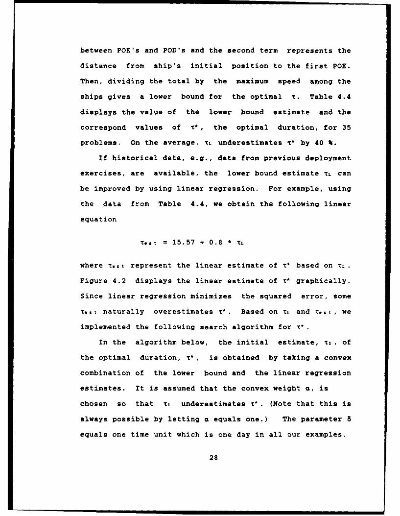
Then, dividing the total by the maximum speed among the
ships gives a lower bound for the optimal C. Table 4.4
displays the value of the lower bound estimate and the
correspond values of C*, the optimal duration, for 35
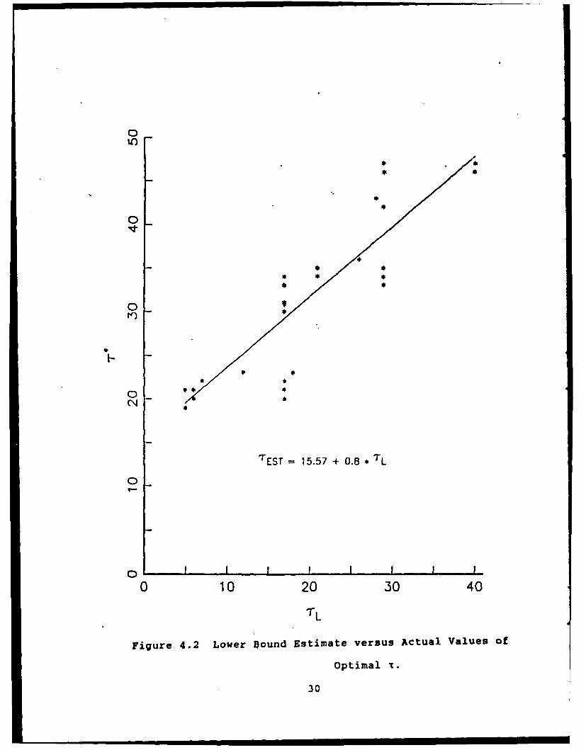
problems. On the average, CL underestimates %* by 40 %.
If historical data, e.g., data from previous deployment
exercises, are available, the lower bound estimate TL can
be improved by using linear regression. For example, using
the data from Table 4.4, we obtain the following linear
equation
-cost = 15.57 + 0.8 * TL
where Test represent the linear estimate of T* based on 'L.
Figure 4.2 displays the linear estimate of V* graphically.
Since linear regression minimizes the squared error, some
Test naturally overestimates T*. Based on TL and -rest, we
implemented the following search algorithm for VC.
In the algorithm below, the initial estimate, xi, of
the optimal duration, V*, is obtained by taking a convex
combination of the lower bound and the linear regression
estimates. It is assumed that the convex weight a, is
chosen so that Ti underestimates T*. (Note that this is
always possible by letting a equals one.) The parameter 6
equals one time unit which is one day in all our examples.
28
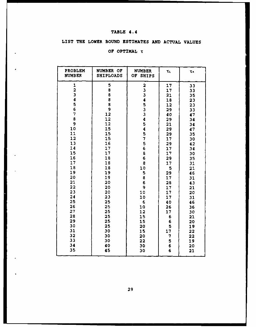
TABLE 4.4
LIST THE LOWER BOUND ESTIMATES AND ACTUAL VALUES
OF OPTIMAL T
PROBLEM NUMBER OF NUMBER TL T*NUMBER SHIPLOADS OF SHIPS
1 5 2 17 332 8 3 17 333 8 3 21 354 8 4 18 235 8 5 12 236 9 3 29 337 12 3 40 478 12 4 29 349 12 5 21 34
10 15 4 29 4711 15 5 29 3512 15 7 17 3013 16 5 29 4214 17 6 17 3415 17 8 17 3016 18 6 29 3517 18 8 17 3118 18 10 5 2119 19 5 29 4620 19 8 17 3121 20 6 28 4322 20 9 17 2123 20 10 17 2024 23 10 17 3125 25 6 40 4626 25 10 26 3627 25 12 17 3028 25 15 6 2129 25 15 6 2030 25 20 5 1931 30 15 17 2232 30 20 7 2233 30 22 5 1934 40 30 6 2035 45 30 6 21
29
0
!0
* *
0-.
o*
0
0 10 20304
$*
'I
* TL
Figure 4.2 Lower Oound Estimate versus Actual Values of
optimal T.30
0 lI I I I
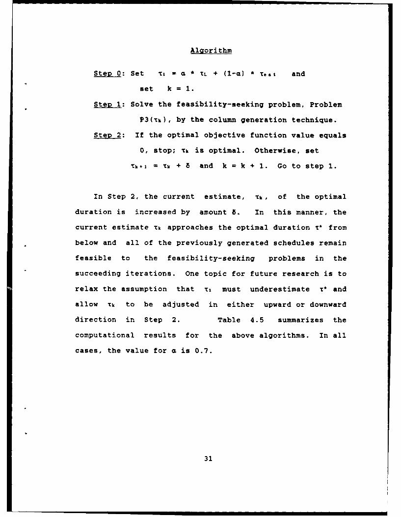
Algorithm
Step 0: Set 'I = C * [L + (1-Q) * test and
set k 1.
Step 1: Solve the feasibility-seeking problem, Problem
P3(Tk), by the column generation technique.
Step 2: If the optimal objective function value equals
0, stop; Ck is optimal. Otherwise, set
Tk 1 = Tk + 5 and k = k + l. Go to step 1.
In Step 2, the current estimate, xk, of the optimal
duration is increased by amount 5. In this manner, the
current estimate 'k approaches the optimal duration V* from
below and all of the previously generated schedules remain
feasible to the feasibility-seeking problems in the
succeeding iterations. One topic for future research is to
relax the assumption that T, must underestimate T* and
allow Ik to be adjusted in either upward or downward
direction in Step 2. Table 4.5 summarizes the
computational results for the above algorithms. In all
cases, the value for a is 0.7.
31
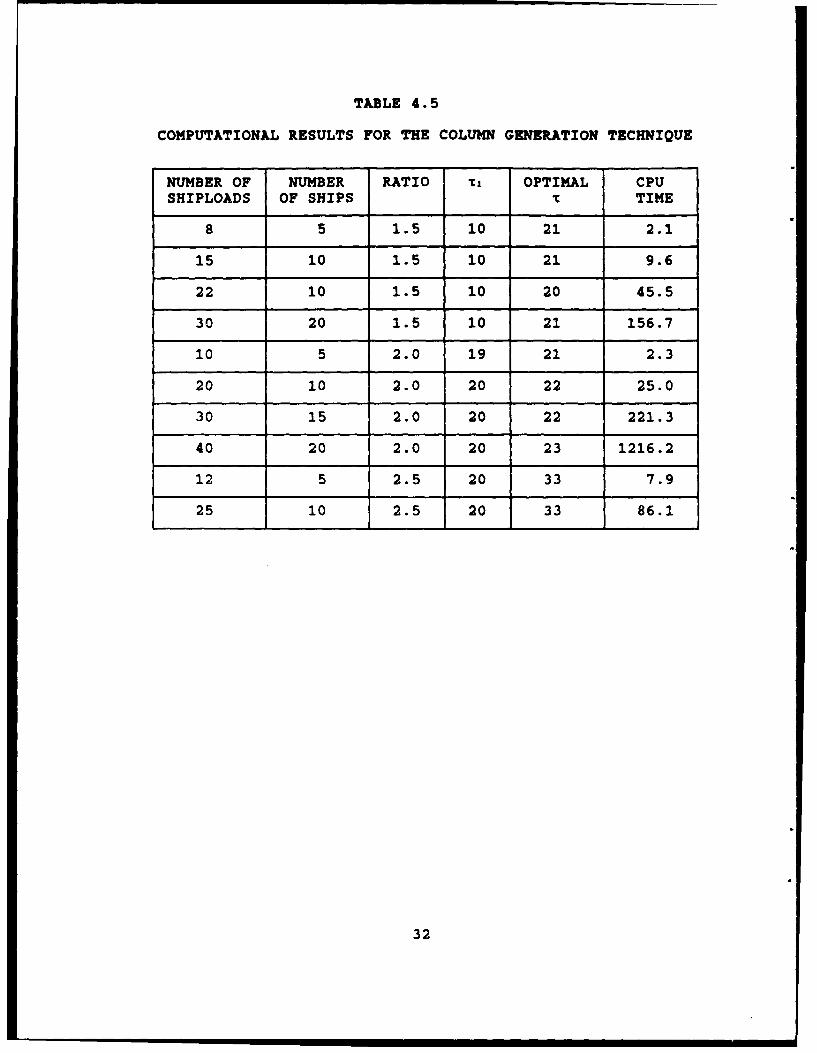
TABLE 4.5
COMPUTATIONAL RESULTS FOR THE COLUMN GENERATION TECHNIQUE
NUMBER OF NUMBER RATIO T1 OPTIMAL CPU
SHIPLOADS OF SHIPS I TIME
8 5 1.5 10 21 2.1
15 10 1.5 10 21 9.6
22 10 1.5 10 20 45.5
30 20 1.5 10 21 156.7
10 5 2.0 19 21 2.3
20 10 2.0 20 22 25.0
30 15 2.0 20 22 221.3
40 20 2.0 20 23 1216.2
12 5 2.5 20 33 7.9
25 10 2.5 20 33 86.1
32
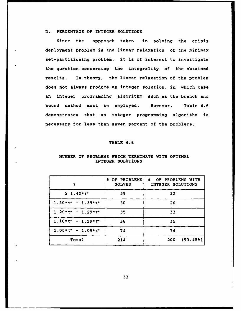
D. PERCENTAGE OF INTEGER SOLUTIONS
Since the approach taken in solving the crisis
deployment problem is the linear relaxation of the minimax
set-partitioning problem, it is of interest to investigate
the question concerning the integrality of the obtained
results. In theory, the linear relaxation of the problem
does not always produce an integer solution, in which case
an integer programming algorithm such as the branch and
bound method must be employed. However, Table 4.6
demonstrates that an integer programming algorithm is
necessary for less than seven percent of the problems.
TABLE 4.6
NUMBER OF PROBLEMS WHICH TERMINATE WITH OPTIMALINTEGER SOLUTIONS
# OF PROBLEMS # OF PROBLEMS WITH
SOLVED INTEGER SOLUTIONS
2 1.40*T* 39 32
1.30*c* - 1.39*rt 30 26
1.20"r* - 1.29*r* 35 33
1.10"t* - 1.19*T* 36 35
1.00*r* - 1.09*r* 74 74
Total 214 200 (93.45%)
33
V. CONCLUSIONS AND FUTURE STUDIES
This study formulates a crisis deployment problem as a
set-partitioning problem with a minimax objective. An
algorithm is developed for solving this problem. The idea
underlying this algorithm is to solve the minimax set-
partitioning by solving a sequence of simpler, but related,
feasibility-seeking problems. Each time the feasibility-
seeking problem produces a better solution for the minimax
problem. The feasibility-seeking problem is similar in
form to the minimax problem and both have a large number of
columns. So to solve the feasibility-seeking problem, the
column generation technique (as in the Dantzig-Wolfe
decomposition method) is employed. The computational
results in Chapter IV verify that this method is effective.
An important by-product of the above development is
that the feasibility-seeking problem can also answer the
question: Can all cargoes be deployed to their final
destinations in x days? A negative answer to this question
leads to two natural follow-up questions which provide
interesting areas for future studies:
1. How many additional ships are required to deploy allcargoes in x days?
2. If no additional ship is available, which cargoesmust be left behind?
34
Besides the above areas and the one mentioned in
Chapter IV, the following areas are also worth studying.
1. The scenario considered in this study assume that thedeployment is completed in one phase. In an extendedperiod of conflicts, one may want deployment plans inseveral phases (waves).
2. Several embellishments to the current model are alsopossible.
a. Allow the cargoes to arrive at the ports withintime windows. The current model assumes that allcargoes are always available for transport.
b. Allow cargoes in partial shiploads and incompatibility among cargoes, e.g., ammunitionshould not be loaded on same ship with fuel.
c. Allow for nondeterministic delays in thecompletion times. These delays are due tounfavorable weather and/or enemy blockade.
35
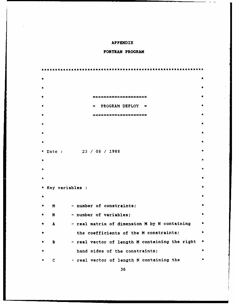
APPENDIX
FORTRAN PROGRAM
• = PROGRAM DEPLOY = *
*Date: 23 /08 / 1988 *
* Key variables: *
' M - number of constraints; *
• N - number of variables; *
* A - real matrix of dimension M by N containing *
• the coefficients of the M constraints; *
• B - real vector of length M containing the right *
• hand sides of the constraints; *
* C - real vector of length N containing the *
36
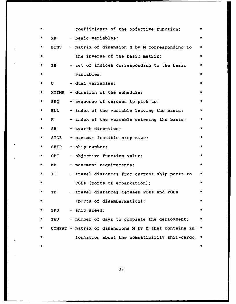
* coefficients of the objective function;
* XB - basic variables; *
* BINV - matrix of dimension M by M corresponding to *
* the inverse of the basic matrix; *
* IB - set of indices corresponding to the basic *
* variables; *
* U - dual variables; a
* XTIME - duration of the schedule; *
* SEQ - sequence of cargoes to pick up; *
* ELL - index of the variable leaving the basis; *
* K - index of the variable entering the basis; *
* SB - search direction; *
* SIGB - maximur feasible step size; *
* SHIP - ship number; a
* OBJ - objective function value; *
* MR - movement requirements; a
* IT - travel distances from current ship ports to *
* POEs (ports of embarkation); *
* TR - travel distances between POEs and PODs *
a (ports of disembarkation); *
* SPD - ship speed; a
a TAU - number of days to complete the deployment; *
a COMPAT - matrix of dimensions M by M that contains in- a
a formation about the compatibility ship-cargo. a
37
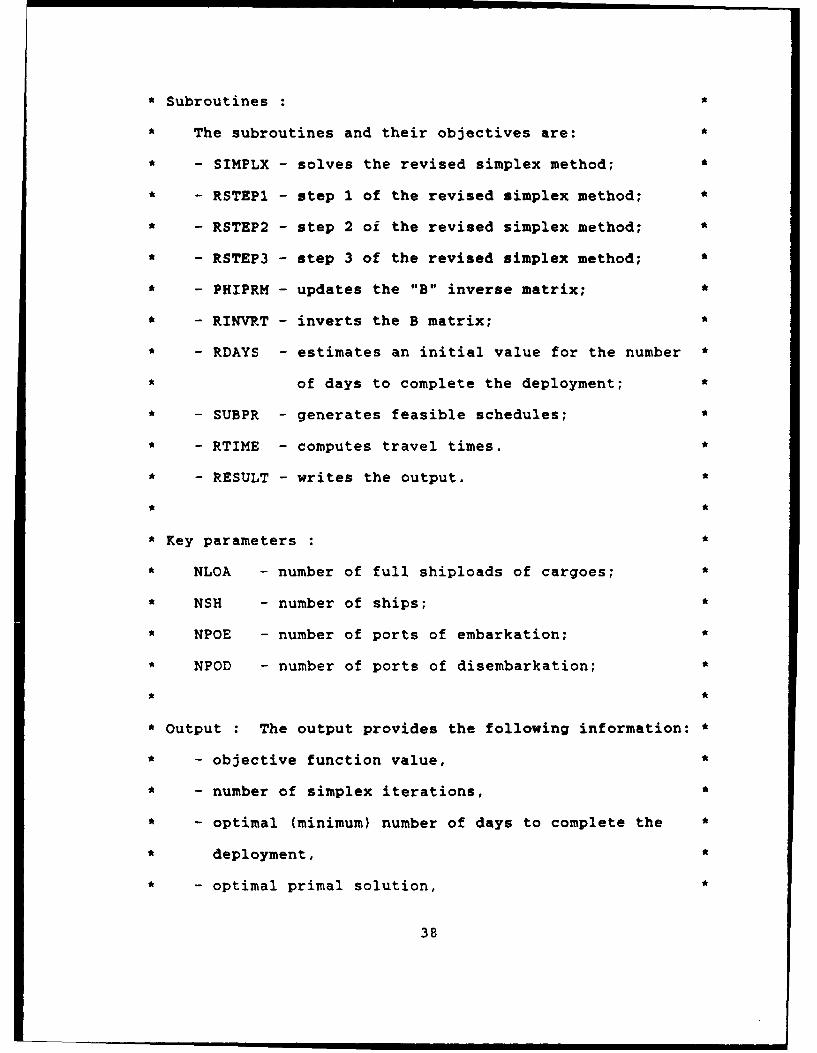
*Subroutines: *
* The subroutines and their objectives are: *
* - SIMPLX - solves the revised simplex method;
* - RSTEP1 -step 1 of the revised simplex method; *
* - RSTEP2 - step 2 oi the revised simplex method; *
* - RSTEP3 - step 3 of the revised simplex method; *
* - PHIPRM -updates the "B" inverse matrix; *
* - RINVRT -inverts the B matrix; *
* - RDAYS - estimates an initial value for the number *
* of days to complete the deployment; *
* - SUBPR -generates feasible schedules; *
* - RTIME - computes travel times. *
* - RESULT - writes the output. *
* Key parameters: *
* NLOA - number of full shiploads of cargoes; *
* NSH - number of ships; *
* NPOE - number of ports of embarkation;
* NPOD - number of ports of disembarkation;
* Output : The output provides the following information: *
* - objective function value, *
* - number of simplex iterations,
* - optimal (minimum) number of days to complete the
* deployment, *
* - optimal primal solution, *
38
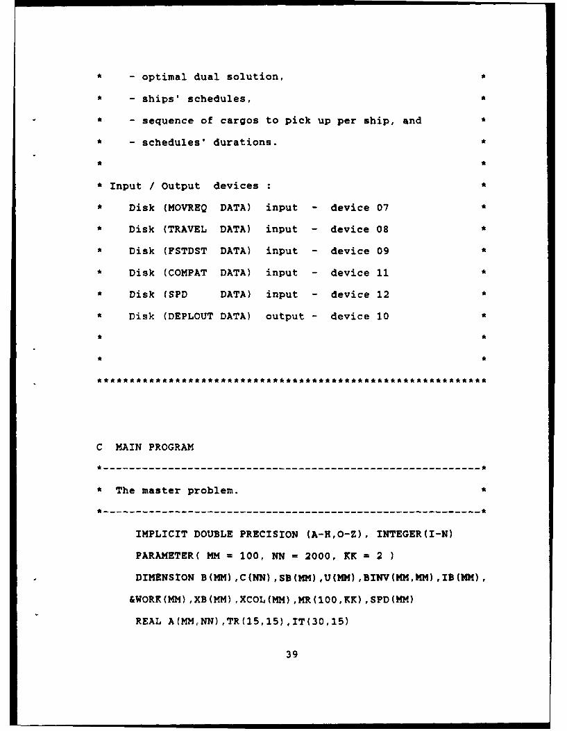
- optimal dual solution, *
- ships' schedules, *
- sequence of cargos to pick up per ship, and *
- schedules' durations. *
* Input / Output devices: *
• Disk (MOVREQ DATA) input - device 07 *
* Disk (TRAVEL DATA) input - device 08 *
* Disk (FSTDST DATA) input - device 09 *
* Disk (COMPAT DATA) input - device 11 *
* Disk (SPD DATA) input - device 12 *
• Disk (DEPLOUT DATA) output - device 10 *
C MAIN PROGRAM
--------------------------------------------------------------------------------- *
* The master problem. *
*--------------------------------------------------------------------------------
IMPLICIT DOUBLE PRECISION (A-H,O-Z), INTEGER(I-N)
PARAMETER( MM = 100, NN = 2000, KK = 2 )
DIMENSION B(MM),C(NN),SB(MM),U(MM),BINV(MM,MM),IB(MM),
&WORK(MM) ,XB(MM) ,XCOL(MM) ,MR(100,KK) ,SPD(MM)
REAL A(MMNN),TR(15,15),IT(30,15)
39
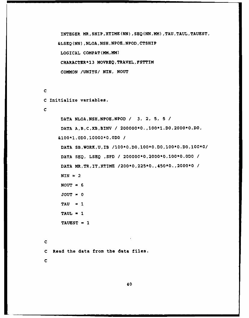
IN'TEGER MR,SHIP,XTIME(NN) PSEQ(NNMM) ITAU,TAUL,TAUEST,
&LSEQ(NN) ,NLOA,NSH,NPOE,NPOD,CTSHIP
LOGICAL COMPAT(MMM*)
CHARACTER* 13 MOVREQ, TRAVEL, FSTTIM
COMMON /UJNITS/ NIN, NOUT
C
C Initialize variables.
C
DATA NLOA,NSH,NPOE,NPOD /3, 2, 5, 5/
DATA A,B,C,XBBINV / 200000*0.,100*1.DO,2000*0.DO,
&100*l.ODO,10000*0.ODO /
DATA SB,WORK,U,IB /100*0 .DO ,100*O.DO ,10O*0.D0 1100*0/
DATA SEQ, LSEQ ,SPD / 200000*0,2000*0,100*0.ODO/
DATA MR,TR,IT,XTIME /200*0,225*0.,450*O.,2000*0/
NIN =2
NOUT =6
JOUT =0
TAU =1
TAUL =1
TAUEST = 1
C
C Read the data from the data files.
C
40
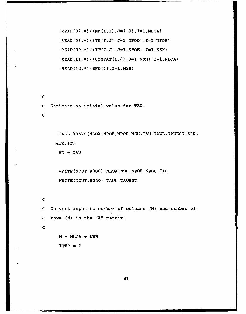
READ (07,*) ((MR (I, J) rJ1, 2),I=1,NLOA)
READ(08,*)((TR(I,J),J=1,NPOD),I=1,NPOE)
READ(09,*) ((IT(I,J),J=1,NPOE),I=l,NSH)
READ(11,*)((COMPAT(I,J),J1,NSH1=1,NLOA)
READ(12,*) (SPD(I) ,I=1,NSH)
C
C Estimate an initial value for TAU.
C
CALL RDAYS(NLOA,NPOE,NPOD,NSH,TAU,TAUL,TAUEST,SPD,
&TR,IT)
MD = TAU
WRITE(NOUT,8000) NLOA,NSH,NPOE,NPOD,TAU
WRITE (NOUT, 8030) TAUL,TAUEST
C
C Convert input to number of columns (M) and number of
C rows (N) in the "A" matrix.
C
M = NLOA + NSH
ITER = 0
41
5000 DO 10 I = 1,MM
B(I) = l.0D0
SB(I = 0.ODO
U(I) = 0.ODO
IBMI = 0
WORK(I = 0..ODO
XB(I) = 1.ODO
XCOL(I = 0.ODO
DO 20 J = 1,NN
C(J) = 0.ODO
XTIME(J) = 0
A(I,J) = 0.
SEQ(J,I) =0
LSEQ(J) =0
20 CONTINUE
DO 30 R=1,MM
BINV(I,K) = .DO
30 CONTINUE
10 CONTINUE
CTSHIP = 0
SHIP = 0
K= 0
N =2*NLOA + NSH
C
C Generate input for the revised simplex method.
42
C
DO 40 I = 1,M
IB(I) = I
DO 50 J = 1,M
IF (I .EQ. J) BINV(I,J) = 1.D0
50 CONTINUE
40 CONTINUE
DO 60 I = 1,M-NSH
C(I) = 1.ODO
60 CONTINUE
C
C Generate artificial variables.
C
DO 70 J = 1,M
DO 80 K = 1,M
IF (J .EQ. K) A(J,K) = 1.
80 CONTINUE
70 CONTINUE
C
C Generate surplus variables.
C
DO 90 J - 1,M
DO 100 K = M+1,2*M-NSH
43
IF(( J .EQ. (K-M) ) .AND. ( J .LE. (M-NSH) ))
& A(J,K)= -1.
100 CONTINUE
90 CONTINUE
SUM = O.Do
DO 110 I=1,M
U(I) =-C(I)
SUM = SUM + C(IB(I))*XB(I)
110 CONTINUE
OBJ = SUM
1000 CONTINUE
C
C Strategy to choose for which ship the next schedule
C will be generated
C
SHIP = SHIP + 1
IF ( SHIP .EQ. NSH + 1 ) SHIP = 1
C
C Generate columns as needed by the master problem.
C
CALL SUBPR(U,XCOLTAU,M,N,NLOA,NPOENPOD,NSHMR,TR,
&IT,A,COMPAT,IBXB,SHIP,XTIME,K,SPDSEQLSEQ,CTSHIP)
DO 120 I = 1, M
44
SUM = 0.ODO
DO 130 J = 1, M
SUM = SUM + BINV(I,J)*A(J,K)
130 CONTINUE
SB(I) = SUM
120 CONTINUE
C
C Perform the revised simplex method.
C
CALL SIMPLX(A,B,C,XB,BINV,SB,U,WORKIB,OBJ,N,MJOUT,
&K,ITER)
IF (OBJ .LT. 10.OD-4) THEN
IF(TAU .EQ. MD) THEN
MD = MD + 10
TAU = TAUL
GO TO 5000
END IF
NT = 1
DO 140 I = 1,M
IF(XB(I) .GT. 1.OD-3 .AND. XB(I) .LT. .9 ) NT=O
140 CONTINUE
WRITE(NOUT,8010) NT
IF(NT .EQ. 1) THEN
GO TO 1100
ELSE
45
IF(ITER .GT. 4000) STOP
GO TO 5000
END IF
END IF
GO TO 1000
C
C Write the results.
C
1100 WRITE(NOUT,8020) TAU
CALL RESULT(JOUT,XB,U,C,A,IB,M,N,OBJ,ITER, SEQ,.LSEQ,
&XTIME,NSHNLOA)
8000 FORMAT(20X, 'PROGRAM OUTPUT' ,/,20X, '--------------',
&//,6X,I2,1X,'SHIPLOADS',3X,12,1X,'SHIPS',3X,I2,
&1X,'POES',3X,I2,1X,'PODS',/,6X,'INITIAL ESTIMATED',
&'VALUE = TAUl = ',12,//)
8010 FORMAT(6X,'NT =',12)
8020 FORMAT(6X,'*** FINAL (OPTIMAL) TAU = ',12)
8030 FORMAT(6X,'** TAUL = ',12,2X,', TAUEST - ',12)
STOP
END
SUBROUTINE SIMPLX (A,BPC,XBIBINV, SB,U,WORK, IB,OBJ,
&N,M,JOUT,K, ITER)
*--------------------------------------------------------------------------------------
46
* This subroutine performs the revised simplex method. *
* ----------------------------------------------------------
IMPLICIT DOUBLE PRECISION (A-H,O-Z), INTEGER(I-N)
PARAMETER( MM = 100, NN - 2000 )
DIMENSION XB(MM),B(MM),C(NN),BINV(MM,MM) ,SB(MM),
&U(MM) ,WORK(MM) ,IB(MM)
REAL A(MM,NN)
INTEGER ELL,XTIME(NN)
COMMON /UNITS/ NIN, NOUT
JOUT = 0
200 'ONTINUE
C
ITER = ITER + 1
IF ( JOUT .EQ. 1 ) RETURN
CALL RSTEP2(XB,SBSIGB,ELL,M,jOUT)
IF ( JOUT EQ. 2 ) RETURN
CALL RSTEP3(XB,C,B,BINVA,WORKOBJoIB,ELL,K,N,M,ITER)
IF (OBJ .LT. 10.OD-4) THEN
NT = 1
DO 10 I - 1,M
IF(XB(I) .GT. 1.OD-3 .AND. XB(I) .LT. .90 ) NT-0
47
10 CONTINUE
IF(NT .EQ. 1) THEN
ITER = ITER + 1
RETURN
END IF
END IF
IF( MOD(ITER,10) .EQ. 0 ) CALL RINVRT(BINV,A,IB,
&WORK,M,N)
CALL RSTEP1(A,C,SB,U,BINV,IB,N,M,K,JOUT)
GO TO 200
END
SUBROUTINE RSTEP1 (A,C,SB,U,BINV,IBN,M,K,JOUT)
*--------------------------------------------------------------------------------------
* This subroutine performs the step one of the revised *
* simplex method *
*---------------------------------------------------------------------------------
IMPLICIT DOUBLE PRECISION (A-H,O-Z), INTEGER(I-N)
PARAMETER( MM = 100, NN = 2000 )
DIMENSION C(NN),SB(MM),U(MM) ,BINV(MM,MM),IB(MM)
REAL A(MM,NN)
48
INTEGER XTIME(NN)
COMMON /UNITS/ NIN, NOUT
C
TOLCON = 1.D-6
JOUT = 0
C
C Compute the duals.
C
DO 10 J=1,M
SUM = 0.DO
DO 20 I=1,M
SUM = SUM + BINV(I,J)*C(IB(I))
20 CONTINUE
10 U(J) = - SUM
C
K = 0
VKMIN = 1.D30
C
DO 50 I=1,N
C
C Check if I is in IB.
C
DO 30 J=1,M
IF( I .EQ. IB(J) ) GO TO 50
30 CONTINUE
SUM = C(I)
49
DO 40 J=I,M
SUM = SUM + A(J,I)*U(J)
40 CONTINUE
IF(SUM .GE. VKMIN) GO TO 50
VKMIN = SUM
K = I
50 CONTINUE
IF(VKMIN .LE. -TOLCON) GO TO 60
JOUT = 1
RETURN
60 CONTINUE
C
C Form SB.
C
DO 80 1=1,M
SUM = 0.DO
DO 70 J=1,M
SUM - SUM + BINV(I,J)*A(J,K)
70 CONTINUE
80 SB(I) = SUM
RETURN
END
50
SUBROUTINE RSTEP2 (XB,SBSIGBELL,M,JOUT)
* ----------------------------------------------------------
This subroutine performs the step two of the revised *
* simplex method *
*--------------------------------------------------------------------------------------
IMPLICIT DOUBLE PRECISION (A-H,O-Z), INTEGER(I-N)
PARAMETER( MM = 100, NN = 2000
DIMENSION XB(MM) ,SB(MM)
INTEGER ELL
COMMON /UNITS/ NIN, NOUT
EPS = 1.D-6
ELL = 0
SIGB = 1.D30
DO 100 I=1,M
IF(SB(I) .LT. EPS) GO TO 100
RATIO = XB(I)/SB(I)
IF(RATIO .GE. SIGB) GO TO 100
SIGB = RATIO
ELL = I
100 CONTINUE
IF(ELL .EQ. 0) JOUT - 2
RETURN
END
51
SUBROUTINE RSTEP3 (XB,CB,BINV,A,WORK,OBJ,IB,ELL,K,
&N,M, ITER)
--------------------------------------------------------------------------------------
* This subroutine performs the step three of the revised *
* simplex method *
------------------------------------------ --------------------------------------------
IMPLICIT DOUBLE PRECISION (A-H,O-Z), INTEGER(I-N)
PARAMETER( MM = 100, NN = 2000)
DIMENSION C(NN) ,XB(MM) ,B(MM) ,BINV(MMMM) ,WORK(MM)
REAL A(MM,NN)
INTEGER ELL,IB(MM)
COMMON /UNITS/ NIN, NOUT
DO 10 I=1,M
10 WORK(I) = A(I,K)
CALL PHIPRM(BINV,WORK,ELL,M)
DO 30 I=1,M
SUM = O.DO
DO 20 J = 1,M
SUM = SUM + BINV(I,J)*B(J)
20 CONTINUE
XB(I) = SUM
30 CONTINUE
IB(ELL) = K
SUM = 0.Do
52
DO 40 1 = I,M
SUM = SUM + C(IB(I))*XB(I)
40 CONTINUE
OBJ = SUM
RETURN
END
SUBROUTINE PHIPRM (BINV,WORK, ELL,M)
*--------------------------------------------------------------------------------------
* This subroutine updates the BINV matrix. *
* ---------------------------------------------------------------- *
IMPLICIT DOUBLE PRECISION (A-H,O-Z), INTEGER (I-N)
PARAMETER( MM =100, NN = 2000
DIMENSION BINV(MM,MM) ,WORK(MM)
INTEGER ELL
COMMON /UNITS/ NIN, NOUT
TOL = 1.D-6
SUM = 0.DO
DO 10 I = i,M
SUM = SUM + BINV(ELL,I)*WORK(I)
10 CONTINUE
YSUM = DABS(SUM)
IF(YSUM .GE. TOL) GO TO 20
53
WRITE(NOUT,8000) SUM
STOP
20 CONTINUE
SUM = 1.DO/SUM
DO 30 I = 1,M
BINV(ELL,I) -SUM*BINV(ELL,I)
IF( (BINV(ELL,I) .LT. TOW) AND. (BINV(ELL,I)
& .GT. -TOL) ) BINV(ELL,I) = 0.ODO
30 CONTINUE
DO 60 J = 1,M
IF(J .EQ. ELL) GO TO 60
TEMP = 0.DO
DO 40 I1 1,M
TEMP =TEMP + BINV(J,I)*WORK(I)
40 CONTINUE
IF( (TEMP .LT. TOLW AND. (TEMP .GT. -TOL)
& TEMP = 0.ODO
DO 50 I = 1,M
BINV(J,I) = BINV(J,I) - TEMP*BINV(ELL,I)
IF( (BINV(J,I) .LT. TOLW AND. (BINV(J,I)
& .GT. -TOL) ) BINV(J,I) = 0.ODO
50 CONTINUE
60 CONTINUE
RETURN
54
8000 FORMAT(6X,'**** ERROR **** NEW MATRIX WOULD BE',
&' SINGULAR, INNER PRODUCT =',G15.6)
END
SUBROUTINE RINVRT (BINV,A,IB,WORK,MN)
*--------------------------------------------------------------------------------------
* This subroutine reinverts the basis. *
*--------------------------------------------------------------------------------------
IMPLICIT DOUBLE PRECISION (A-H,O-Z), INTEGER(I-N)
PARAMETER ( ZERO = 0.ODO, ONE = 1.ODO
PARAMETER ( MM =100, NN = 2000 )
DIMENSION BINV(MM,MM), IB(MM), OMAT(MM,MM), WORK(MM)
REAL A(MM,NN)
COMMON /UNITS/ NIN, NOUT
TOL = 1.D-6
DO 10 I = 1, M
DO 20 J = 1, M
BINV(I,J) = ZERO
OMAT(I,J) = A(I,IB(J))
20 CONTINUE
BINV(I,I) = ONE
10 CONTINUE
C
55
C Locate maximum magnitude element on or below the main
C diagonal.
C
DO 30 K = 1, M
IF ( K .LT. M) THEN
IMAX = K
AMAX = DABS(OMAT(K,K))
KP1 = K+1
DO 40 I = KPl, M
IF ( AMAX .LT. DABS(OMAT(I,K))) THEN
IMAX = I
AMAX = DABS(OMAT(I,K))
ENDIF
40 CONTINUE
C
C Interchange rows IMAX and K if IMAX is not equal to K
C
IF (IMAX .NE. K) THEN
DO 50 J 1, M
ATMP = OMAT(IMAX, J)
OMAT(IMAX, 3) = OMAT(K,J)
OMAT(KJ) = ATMP
BTMP = BINV(IMAX,J)
BINV(IMAX,J) = BINV(K,J)
BINV(K,J) = BTMP
56
50 CONTINUE
ENDIF
ENDIF
C
C Test for singular matrix.
C
IF (DABS(OMAT(K,K)) .LT. 1.OD-6) THEN
WRITE(NOUT,8000) K, OMAT(K,K)
ELSE
DIV = OMAT(K,K)
DO 60 J = 1, M
OMAT(K,J) = OMAT(K,J)/DIV
IF( (OMAT(K,J) .LT. TOL) .AND. (OMAT(K,J)
& .GT. -TOL) )OMAT(K,J) = 0.ODO
BINV(K,J) =BINV(K,J)/DIV
IF( (BINV(K,J) .LT. TOL) AND. (BINV(K,J)
& .GT. -TOL) ) BINV(K,J) = 0.ODO
60 CONTINUE
DO 70 I = 1, M
AMULT = OMAT (I, K)
IF( (AMULT .LT. TOL) AND. (ANULT
& .GT. -TOL) ) AMULT - O.ODO
IF ( I .NE. K) THEN
DO 80 J - 1, M
OMAT(I,J) = OMAT(I,J) - AMULT
57
& * OMAT (K, J)
BINV(I,J) = BINV(I,J) - AMULT
& * BINV(K,J)
IF( (BINV(I,J) .LT. TOL) .AND.
& (BINV(I,J) .GT. -TOL
& BINV(I,J) = O.ODO
80 CONTINUE
ENDIF
70 CONTINUE
ENDIF
30 CONTINUE
8000 FORMAT(' * ERROR: BASIS IS SINGULAR',14,D5.6)
RETURN
END
SUBROUTINE SUBPR (U,XCOL,TAU,M,N,NLOA,NPOE,NPOD,NSH,
&MR,TRIT,A,COMPAT,IB,XB,SHIP,XTIME,K,SPD,SEQ,LSEQ,
&CTSHIP)
*--------------------------------------------------------------------------------------
• This subroutine generates feasible (acceptable) columns *
*--------------------------------------------------------------------------------------
IMPLICIT DOUBLE PRECISION (A-H,O-Z), INTEGER (I-N)
PARAMETER( MM = 100, NN = 2000, KK = 2, JJ = --00
DIMENSION XCOL(MM),U(MM),UU(MM),V(MM),XB(MM),SA(MM),
&IB(MM),SPD(MM)
58
REAL A(MM,NN),TR(15,15),IT(30.15)
INTEGER VIND(MM),PRED(O:JJ),LOAD(0:JJ),TIME(0:JJ),
& MR(100,KK),FROLD,TOLD,PATH(0:MM),CURLDUCOUNT,
& LENGTH,LASTND, SHIP,TT,MLNGTH,XTIME(NN) ,CTSHIP,
& CTSON(O:MLLSEQ(NN),TAU,STACK(0:JJ),TOP,
& SEQ(NN,MM) ,CTBACK(O:MM)
LOGICAL COMPAT(MMPMM)
DOUBLE PRECISION MIN,MINRC
COMMON /UNITS/ NIN,NOUT
C
C Initialize the variables.
C
LIMIT =N
1000 CTSHIP =0
2000 DO 10 1 1,MM
SACI) = 0.0D0
UU(I) = 0.DO
V(I) = 0.D0
VIND(I) = 0
10 CONTINUE
NNEG = NLOA
MINRC = 0.ODO
C
C Sort the duals.
59
C
DO 20 I = 1,NLOA
UU(I) = U(I)
20 CONTINUE
IF( N .GE. (2*NLOA + NSH + 1) ) THEN
DO 30 I= 1,M
DO 40 J = 1,M
IF( (IB(J) .GT. (2*NLOA + NSH)) .AND.
& (A((NLOA + SHIP),IB(J)) .NE. 1.D0) .AND.
& (XB(J) .GT. 0.5D0) ) THEN
SA(I) = SA(I) + A(IIB(J))
END IF
40 CONTINUE
IF( SA(I) .LT. 1.ODO ) UU(I) = -2.ODO
30 CONTINUE
END IF
C
C Check ship-cargo and ship-port compatibility.
C
DO 50 I = 1,NLOA
IF( .NOT. COMPAT(I,SHIP) ) UU(I) = 99.ODO
50 CONTINUE
DO 60 I = 1,NLOA
MIN - 0.1D-6
COUNT = 0
IND = 0
60
DO 70 J = 1,NLOA
IF( UU(J) .LT. MIN ) THEN
MIN = UU(J)
IND = J
COUNT = 1
END IF
70 CONTINUE
IF( COUNT .EQ. 0 ) THEN
NNEG = I - 1
GO TO 4000
END IF
V(I) = MIN
VIND(I) = IND
UU(IND) = 99.ODO
60 CONTINUE
4000 CONTINUE
C
C The Modified Depth First Search Algorithm.
C
C
C Create all nodes out of the source and include them
C in a stack.
61
C
DO 80 I =O,JJ - 1
TIME(I) = 0
STACK(I) = 0
LOAD(I) = 0
PRED(I) = 0
80 CONTINUE
DO 90 I = 1,MM
XCOL(I = O.DO
PATH(I-1) = 0
CTBACK(I-1) =0
CTSON(I-1) =0
90 CONTINUE
LENGTH = 0
LASTND = 1
TOP = 0
CURLD = 0
FROLD = 0
TOLD = 0
DO 100 1 = NNEG,1,-1
LOAD(NNEG - I + 2) = VIND(I)
PRED(NNEG - I + 2) = 1
STACK(NNEG - I + 1) =(NNEG 1 2)
TOP = TOP + 1
LASTND = LASTND + 1
62
IF( CTSON(LENGTH) .EQ. CTBACK(LENGTH) ) THEN
DO 150 I = 1,LENGTH
IF( PRED(CURLD) .EQ. PATH(I) ) THEN
LASTND = LASTND - LENGTH + I
LENGTH = I
GO TO 5000
END IF
150 CONTINUE
END IF
5000 PATH(LENGTH + 1) = CURLD
C
C Compute the travel time to pick up another cargo.
C
FROLD = LOAD(PRED(CURLD))
TOLD = LOAD(CURLD)
TT = 0
CALL RTIME(NPOE,NPOD,MR,TR,IT,FROLD,TOLDSHIP,NSH,
&NLOA,TT,SPD)
TIME(CURLD) = TIME(PRED(CURLD)) + TT
C
C Verify if it is feasible to pick up another cargo.
C
65
IF( TIME(CURLD) .LE. TAU ) THEN
CTBACK(LENGTH) = CTBACK(LENGTH) + 1
LENGTH = LENGTH + 1
CTSON(LENGTH) =0
DO 160 I = NEG,1,-1
DO 170 J = 1, LENGTH
IF( VIND(I) EQ. LOAD(PATH(J)) )GO TO 160
170 CONTINUE
LASTND = LASTND + 1
LOAD(LASTND) = VIND(I)
PRED(LASTND) = CURLD
TOP = TOP + 1
CTSON(LENGTH) = CTSON(LENGTH) + 1
160 CONTINUE
DO 180 I = LASTND,(LASTND - CTSON(LENGTH)+1),-l
STACK(TOP) =I
TOP = TOP -1
180 CONTINUE
TOP = TOP + CTSON(LENGTH)
ELSE
LASTND =LASTND - 1
RCOST = .ODO
DO 190 I = 1,LENGTH
XCOL(LOAD(PATH(I))) = 1.ODO
190 CONTINUE
XCOL(NLOA + SHIP) = 1.ODO
66
DO 200 I = 1,M
IF( XCOL(I) .EQ. 1.ODO ) RCOST = RCOST + U(I)
200 CONTINUE
IF(RCOST .GT. -1.OD-4) RCOST = 0.0D0
IF( RCOST .LT. O.ODO .AND. LENGTH .GT.
& INT(NLOA/NSH)-1 ) THEN
IF ( CTBACK(LENGTH) .EQ. 0 ) THEN
N = N + 1
DO 210 I = 1,M
A(I,N) = XCOL(I)
210 CONTINUE
XTIME(N) = TIME(PRED(CURLD))
DO 220 J = 1,LENGTH
SEQ(N,J) = LOAD(PATH(J))
220 CONTINUE
LSEQ(N) = LENGTH
IF( RCOST .LT. MINRC ) THEN
MINRC = RCOST
KE= N
END IF
END IF
DO 230 I = 1,LENGTH
XCOL(LOAD(PATH(I))) = 0.0D0
XCOL(NLOA + SHIP) = 0.0D0
230 CONTINUE
ELSE
67
DO 240 I = 1,LENGTH
XCOL(LOAD(PATH(I))) = 0.ODO
240 CONTINUE
XCOL(NLOA + SHIP) = O.ODO
END IF
CTBACK(LENGTH) = CTBACK(LENGTH) + 1
GO TO 3000
END IF
IF( N .GE. LIMIT + 1 ) RETURN
CTBACK(LENGTH) = 0
GO TO 3000
8000 FORMAT(//,6X,'TAU NOT FEASIBLE, INCREASE TAU '
8010 FORMAT(/,6X,'NEW TAU = ',14)
END
SUBROUTINE RTIME (NPOE,NPOD,MRTR, IT, FROLD,TOLD, SHIP,
&NSHNLOA,TT, SPD)
*--------------------------------------------------------------------------------------
*This subroutine calculates travel times.*
*--------------------------------------------------------------------------------------
IMPLICIT DOUBLE PRECISION( A-H,O-Z ), INTEGER( I-N
PARAMETER( KK = 2, MM = 100, NN = 2000
DIMENSION SPD(MM)
REAL IT(30,15),TR(15,15)
INTEGER MR(100,KJK),TT,TOLD,SHIP,FROLD
68
TT = 0
C Calculating the travel time.
IF(FROLD .EQ. 0) THEN
TT = IDNINT((IT(SHIP,MR(TOLD,1)) + TR(MR(TOLD,1),
& MR(TOLD,2))) / (24. * SPD(SHIP)))
ELSE
TT = IDNINT((TR(MR(TOLD,1),MR(FROLD,2)) +
& TR(MR(TOLD,1),MR(TOLD,2)))/(24. * SPD(SHIP)))
END IF
RETURN
END
SUBROUTINE RDAYS (NLOA,NPOENPOD,NSH,TAU,TAUL,
&TAUEST, SPD ,TR,IT)
*--------------------------------------------------------------------------------------
*This subroutine calculates an initial estimate of the
*number of days to complete the deployment.*
*--------------------------------------------------------------------------------------
PARAMETER ( MM = 100)
INTEGER NPOE,NPOD,TAU,TAUL,TAUEST,NLOA,NSH
DIMENSION TR(15,15), IT(30,15)
REAL TRITTTI,SPMAX
69
DOUBLE PRECISION SPD(MM)
COMMON /UNITS/ NINNOT
TAU =1
TAUJ 1
TAUEST = 1
C
C Calculate the minimum distance to travel.
C
TRMIN = 99999999.
DO 100 I=1,NPOE
DO 200 J=1,NPOD
IF(TR(I,J) .LT. TRMIN) TRMIN = TR(I,J)
200 CONTINUE
100 CONTINUE
C
C Calculate the minimum travel distance from the initial
C ships' locations to the POEs.
C
ITMIN = 99999999.
DO 300 I - 1,NSH
DO 400 J = 1,NPOE
IF(IT(I,J) .LT. ITMIN) ITMIN - IT(I,J)
400 CONTINUE
300 CONTINUE
70
C
C Calculate the maximum traveling ships' speeds.
C
SPMAX = -1.
DO 600 J = 1,NSH
IF(SPD(J) .GT. SPMAX) SPMAX - SPD(J)
600 CONTINUE
C
C Compute the average number of trips per ship.
C
NTR = NLOA / REAL(NSH)
C
C Calculate an estimate for TAU.
C
TAUL = INT(((((NTR * 2) - 1) * TRMIN) + ITMIN) /
& (SPMAX*24.))
TAUEST = INT(15.5 + 0.8 * TAUL ))
TAU = INT( (0.7 * TAUL) + (0.3 * TAUEST)
RETURN
END
71
SUBROUTINE RESULT (JOUT,XB,U,C,A,IB,M,N,OBJ,ITER,
&SEQ,LSEQ,XTIME,NSH,NLOA)
*--------------------------------------------------------------------------------------
* This subroutine writes the solution to the output file *
* ---------------------------------------------------------- *
IMPLICIT DOUBLE PRECISION(A-H, O-Z), INTEGER(I-N)
PARAMETER( MM =100, NN = 2000, ZERO = 0.ODO
DIMENSION U(MM),C(NN),XB(MM),IB(MM)
INTEGER SEQ(NN,MM),LSEQ(NN),XTIME(NN)
REAL A(MM,NN)
COMMON /UNITS/ NIN, NOUT
IF(JOUT .GE. 2) GO TO 80
WRITE(NOUT,8000) OBJ
WRITE(NOUT,8005) ITER
WRITE(NOUT,8010)
C
C Is X(I) basic?
C
DO 30 I=1,N
DO 10 J=1,M
INDEX - J
IF(IB(J) .EQ. I) GO TO 20
10 CONTINUE
GO TO 30
72
20 CONTINUE
WRITE(NOUT,8020) I.XB(INDEX)
30 CONTINUE
WRITE (NOUT, 8030)
WRITE(NOUT,8040) (I,U(I) ,I=1,NLOA)
WRITE(NOUT,8050) (IU(I),I=(NLOA+1),M)
Do 70 11I,N
DO 40 J=1,M
IF(IB(J .EQ. IV THEN
IF((XB(J) .GT. 1.D-2) .AND. (I .GT.
& 2*NLOA+NSH)) THEN
DO 90 L=NLOA+1,M
IF( A(L,IB(J)) .GT. .9)
& WRITE(NOUT,9010) (L-NLOA)
90 CONTINUE
WRITE(NOUT,9020) (SEQ(IB(J),K),
& K = 1,LSEQ(IB(J)))
WRITE(NOUT,8090) IB(J),XTIME(IB(J))
END IF
GO TO 60
END IF
40 CONTINUE
C
C X(I) is non basic.
C
73
sum = C (I)
DO 50 J=1,M
SUM = SUM + A(J,I)*U(J)
50 CONTINUE
GO TO 70
C
C X(I) is basic.
C
60 CONTINUE
70 CONTINUE
80 CONTINUE
IF(JOUT .EQ. 2) WRITE(NOUT,8070)
IF(JOUT .EQ. 3) WRITE(NOUT,8080)
RETUR14
C
8000 FORMAT(//,6X,'OPTIMAL OBJECTIVE FUNCTION VALUE IS',
&F12. 5)
8005 FORMAT(//,6X,'NUMBER OF ITERACTIONS = ',15)
8010 FORMAT(//,17X, 'OPTIMAL PRIMAL SOLUTION',!)
8020 FORMAT(18X,'X(',I3,') =',F14.7)
8030 FORMAT(//,18X, 'OPTIMAL DUAL SOLUTION',!)
8040 FORMAT(18X,'U(',I2,I) =',Fl4.7)
8050 FORMAT(18X,'V(',12,l) -',Fl4.7)
8070 FORMAT(//,6X,'PROBLEM IS UNBOUNDED FROM BELOW')
8080 FORMAT(//,6X,'PROBLEM HAS NO FEA'SIBLE SOLUTION')
74
8090 FORMAT(6X,'DURATION OF SCHEDULE ',14,' IS :',13,/)
9010 FORMAT(/,6X, 'SCHEDULE FOR SHIP ',12,/,6X, 'CARGOES
&TO CARRY:')
9020 FORMAT(6XI4)
END
75
LIST OF REFERENCES
1. Ronen, D., "Cargo Ships Routing and Scheduling: Surveyof Models and Problems", European Journal of OperationsResearch, Vol. 12, 1983.
2. Brown, G. G., Graves, G. W., and Ronen, D., "SchedulingOcean Transportation of Crude Oil", Manaaement Science,Vol. 33, No. 3, March 1987.
3. Goodman, C. E., Annual Scheduling of Atlantic FleetNaval Combatants, M.S. Thesis, Naval PostgraduateSchool, Monterey, CA, March 1985.
4. Collier, K. S., Deployment Planning: A LinearProgramming Model With Variable Reduction, M.S.Thesis, Naval Postgraduate School, Monterey, CA,September 1987.
5. Ketron Management Science, Inc., MPS III MathematicalProgramming System-General Description, January 1987.
6. Lally, M., Strategic Allocation of Sealift: A GAMS-Based Intecer Programming Approach, M.S. Thesis, NavalPostgraduate School, Monterey, CA, September 1987.
7. Brooke A., Kendrick D. and Meeraus A., GAMS - A User'sGuide, The Scientific Press, CA, 1988.
8. Lasdon, L.S., Optimization Theory for Large Systems,Macmillan, New York, 1979.
9 Buvik, Svein, An Algorithm for Generating ShipSchedules for a Crisis Deployment Planning Problem,M.S. Thesis, Naval Postgraduate School, Monterey, CA,September 1988.
10. Best, M.J, and Ritter, K., Linear Programming Activeset Analysis and Computer Programs, Prentice-Hall Inc.,New Jersey, 1985.
76
INITIAL DISTRIBUTION LIST
No. Copies
1. Defense Technical Information Center 2Cameron StationAlexandria, Virginia 22304-6145
2. Library, Code 0142 2Naval Postgraduate SchoolMonterey, California 93943-5002
3. Professor Siriphong Lawphongpanich, Code 55Lp 6Department of Operations ResearchNaval Postgraduate SchoolMonterey, California 93943
4. Professor Richard E. Rosenthal, Code 55R1 1Department of Operations ResearchNaval Postgraduate SchoolMonterey, California 93943
5. LT Carlos Vallejo, Code 30 2Operation Research Curricular OfficeNaval Pcstgraduate SchoolMonterey, California 93943
6. LT Francisco W. Taborda 2SMC #1145Naval Postgraduate SchoolMonterey, California 93943-5000
7. Lt. Cdr. Newton Rodrigues Lima 2Brazilian Naval Commission4706 Wisconsin Avenue, N. W.Washington, D.C. 20016
8. Lt. Cdr. Svein Buvik 2FO/SST/ORG 3Oslo mil/Huseby0016 Oslo 1Norway
9. Vice Admiral Edson Ferracciu 2Comando do Segundo Distrito Naval4706 Wisconsin Ave., N. W.Washington, D.C. 20016
10. Brazilian Naval Commission 54706 Wisconsin Ave., N. W.Washington, D.C. 20016
77