NAVAL POSTGRADUATE SCHOOL - apps.dtic.mil · i REPORT DOCUMENTATION PAGE Form Approved OMB No. 0704-0188 Public reporting burden for this collection of information is estimated to

NAVAL

POSTGRADUATE SCHOOL

MONTEREY, CALIFORNIA

THESIS

Approved for public release; distribution is unlimited

REDEFINING THE AUSTRALIAN ARMY OFFICER CORPS ALLOCATION PROCESS

by

David G. Nelson

March 2010

Thesis Co-Advisors: William Gates William Hatch

i

REPORT DOCUMENTATION PAGE Form Approved OMB No. 0704-0188 Public reporting burden for this collection of information is estimated to average 1 hour per response, including the time for reviewing instruction, searching existing data sources, gathering and maintaining the data needed, and completing and reviewing the collection of information. Send comments regarding this burden estimate or any other aspect of this collection of information, including suggestions for reducing this burden, to Washington headquarters Services, Directorate for Information Operations and Reports, 1215 Jefferson Davis Highway, Suite 1204, Arlington, VA 22202-4302, and to the Office of Management and Budget, Paperwork Reduction Project (0704-0188) Washington DC 20503.

1. AGENCY USE ONLY (Leave blank)

2. REPORT DATE March 2010

3. REPORT TYPE AND DATES COVERED Master’s Thesis

4. TITLE AND SUBTITLE Redefining the Australian Army Officer Corps Allocation Process

6. AUTHOR(S) David. G. Nelson

5. FUNDING NUMBERS

7. PERFORMING ORGANIZATION NAME(S) AND ADDRESS(ES) Naval Postgraduate School Monterey, CA 93943-5000

8. PERFORMING ORGANIZATION REPORT NUMBER

9. SPONSORING /MONITORING AGENCY NAME(S) AND ADDRESS(ES) N/A

10. SPONSORING/MONITORING AGENCY REPORT NUMBER

11. SUPPLEMENTARY NOTES The views expressed in this thesis are those of the author and do not reflect the official policy or position of the Department of Defense or the U.S. Government.

12a. DISTRIBUTION / AVAILABILITY STATEMENT Approved for public release; distribution is unlimited

12b. DISTRIBUTION CODE

13. ABSTRACT (maximum 200 words)

Data was obtained from 6,114 United States Marine Corps (USMC) Officers who graduated from The Basic School (TBS). The USMC data was used to conduct regression analysis on how Military Occupational Specialties (MOS) allocation affects retention. The regression model that was developed was a linear probability model. The results from the regression showed that retention was positively affected by receiving your first MOS preference and negatively affected by receiving an MOS outside your top three preferences. The USMC MOS allocation process is very similar to the Australian Army’s corps allocation process and the voluntary nature of military service in both countries enables comparisons to be drawn. Within the Australian Army, both the strength and the direction of the variable affects would be similar to those in the USMC.

Optimization models were developed that maximized cadet preferences whilst also meeting service requirements. Data from cadets who graduated from the Royal Military College in 2008 and 2009 was utilized to assess four different optimization models. The models that were developed showed significant increases in those cadets who received their first or second preference and significant decreases in cadets being allocated to the third, fourth or other preferences.

15. NUMBER OF PAGES

111

14. SUBJECT TERMS Retention, Australian Army, Optimization Models, Royal Military College, Officers, Manpower, Corps Allocation, Military Occupational Specialties (MOS) Allocation, MOS retention.

16. PRICE CODE

17. SECURITY CLASSIFICATION OF REPORT

Unclassified

18. SECURITY CLASSIFICATION OF THIS PAGE

Unclassified

19. SECURITY CLASSIFICATION OF ABSTRACT

Unclassified

20. LIMITATION OF ABSTRACT

UU

NSN 7540-01-280-5500 Standard Form 298 (Rev. 2-89) Prescribed by ANSI Std. 239-18

ii

THIS PAGE INTENTIONALLY LEFT BLANK

iii

Approved for public release, distribution is unlimited

REDEFINING THE AUSTRALIAN ARMY OFFICER CORPS ALLOCATION PROCESS

David G. Nelson Major, Royal Australian Army Medical Corps

B.A, New South Wales University, 1997 MBA, Southern Cross University, 2001

Submitted in partial fulfillment of the requirements for the degree of

MASTER OF SCIENCE IN MANAGEMENT

from the

NAVAL POSTGRADUATE SCHOOL March 2010

Author: David G. Nelson

Approved by: William Gates Thesis Co-Advisor

William Hatch Thesis Co-Advisor

William Gates Dean, Graduate School of Business and Public Policy

iv


v

ABSTRACT

Data was obtained from 6,114 United States Marine Corps (USMC) Officers who

graduated from The Basic School (TBS). The USMC data was used to conduct regression

analysis on how Military Occupational Specialties (MOS) allocation affects retention.

The regression model that was developed was a linear probability model. The results

from the regression showed that retention was positively affected by receiving your first

MOS preference and negatively affected by receiving an MOS outside your top three

preferences. The USMC MOS allocation process is very similar to the Australian Army’s

corps allocation process and the voluntary nature of military service in both countries

enables comparisons to be drawn. Within the Australian Army, both the strength and the

direction of the variable affects would be similar to those in the USMC.

Optimization models were developed that maximized cadet preferences whilst

also meeting service requirements. Data from cadets who graduated from the Royal

Military College in 2008 and 2009 was utilized to assess four different optimization

models. The models that were developed showed significant increases in those cadets

who received their first or second preference and significant decreases in cadets being

allocated to the third, fourth or other preferences.

vi


vii

TABLE OF CONTENTS

I. INTRODUCTION........................................................................................................1 A. BACKGROUND ..............................................................................................1 B. PURPOSE.........................................................................................................1 C. CONTEXT........................................................................................................2 D. DATA ................................................................................................................2 E. SCOPE AND METHODOLOGY ..................................................................3

II. LITERATURE REVIEW ...........................................................................................5 A. OVERVIEW.....................................................................................................5 B. WORK-RELATED FACTORS......................................................................7 C. INDIVIDUAL CHARACTERISTICS...........................................................9 D. MILITARY SPECIFIC.................................................................................12 E. LITERATURE SUMMARY.........................................................................15

III. REGRESSION ANALYSIS OF UNITED STATES MARINE CORPS OFFICERS .................................................................................................................17 A. PURPOSE.......................................................................................................17 B. COMMISSIONING PROGRAMS...............................................................17

1. The United States Naval Academy (USNA).....................................17 2. Naval Reserve Officer Training Course (NROTC) ........................17 3. Platoon Leaders Course (PLC).........................................................18 4. Officer Candidate Course (OCC).....................................................18 5. Marine Corps Enlisted Commissioning Program (MECEP).........18 6. Enlisted Commissioning Program (ECP) ........................................19 7. Meritorious Commissioning Program (MCP).................................19

C. COMMON MARINE CORPS OFFICER TRAINING .............................20 D. DATA AND VARIABLES ............................................................................21

1. Center for Naval Analyses (CNA) ....................................................21 2. Total Force Data Warehouse (TFDW) ............................................21

E. REGRESSION ANALYSIS ..........................................................................22 F. SUMMARY AND CONCLUSION ..............................................................32

IV. ROYAL MILITARY COLLEGE MODELING ANALYSIS ...............................35 A. SCOPE ............................................................................................................35 B. BACKGROUND ............................................................................................35 C. CURRENT PROCESS ..................................................................................36 D. OPTIMIZATION MODELING...................................................................37

1. Decision Variables..............................................................................39 2. Objective Function.............................................................................39 3. Defining Constraints..........................................................................39 4. Interpreting Solver Solutions............................................................40

E. DATA ..............................................................................................................40 1. 2008 Data ............................................................................................40

viii

2. 2009 Data ............................................................................................45 F. MODEL ASSESSMENT...............................................................................49 G. MODEL 1 (WEIGHTED FOR CADET PREFERENCE).........................50 H. MODEL 2 (FIRST OR SECOND CHOICE CORPS GUARANTEE).....57 I. MODEL 3 (ALLOCATED BY QUEENS MEDAL ORDER) ...................63 J. MODEL 4 (WEIGHTED FOR CADET PREFERENCE AND

QUEENS MEDAL SCORE) .........................................................................70 K. MODEL SUMMARY ....................................................................................80

V. SUMMARY, CONCLUSIONS AND RECOMMENDATIONS ...........................83 A. SUMMARY ....................................................................................................83 B. CONCLUSIONS AND RECOMMENDATIONS.......................................87 C. RECOMMENDATION FOR FURTHER STUDY ....................................88

LIST OF REFERENCES......................................................................................................89

INITIAL DISTRIBUTION LIST .........................................................................................91

ix

LIST OF FIGURES

Figure 1. Solver Parameters ............................................................................................38 Figure 2. 2008 and 2009 Queens Medal Average (Original Allocation and Model 3)...69 Figure 3. 2008 and 2009 Queens Medal Average (Original Allocation and Model 4)...79

x


xi

LIST OF TABLES

Table 1. Variable Effect and Variable Strength.............................................................11 Table 2. Summary of Military Turnover Variables (From Burch, Conroy, & Bruce,

1991) ................................................................................................................13 Table 3. Summary of Active Service MSO ...................................................................19 Table 4. Variable Description ........................................................................................22 Table 5. Descriptive Statistics........................................................................................24 Table 6. Regression Results: Retained to Six Years after Commissioning ...................30 Table 7. Regression Significance: Retained to Six Years after Commissioning...........31 Table 8. Corps Preferences and Allocation (2008) ........................................................41 Table 9. Actual Preference Achievement (2008)...........................................................44 Table 10. Graphical Preference Achievement (2008)......................................................44 Table 11. Cadet Preferences and Corps Allocation for RMC (2009) ..............................45 Table 12. Preference Achievement (2009) ......................................................................47 Table 13. Graphical Preferences Achievement (2009) ....................................................48 Table 14. Preference Achievement (2008 and 2009).......................................................48 Table 15. Graphical Preferences Achievement (2008 /2009) ..........................................49 Table 16. Decision Variables (Model 1)..........................................................................50 Table 17. Constraints (Model 1) ......................................................................................51 Table 18. 2008 Weightings and Preference Achievement (Model 1)..............................52 Table 19. 2008 Preference Achievement (Original Allocation and Model 1) .................53 Table 20. 2009 Preference Achievement (Original Allocation and Model 1) ................54 Table 21. Model 1 Preference Achievement (2008 and 2009 Combined).......................55 Table 22. Model 1 Performance.......................................................................................56 Table 23. Model 2 Corps Breakdown (2008) ..................................................................58 Table 24. Model 2 Preference Achievement (2008) ........................................................58 Table 25. 2009 Corps Breakdown (Model 2) ..................................................................59 Table 26. 2009 Preference Achievement (Model 2) ........................................................59 Table 27. 2009 Revised Corps Allocation Numbers (Model 2) ......................................60 Table 28. 2009 Revised Corps Allocation Overage and Underage (Model 2) ................61 Table 29. 2009 Preference Achievement (Model 2 Revision).........................................62 Table 30. Model 2 Preference Achievement (2008 and 2009 Combined).......................62 Table 31. Model 2 Performance.......................................................................................63 Table 32. 2008 Preference Achievement (Original Allocation and Model 3) .................65 Table 33. 2008 Queens Medal Average (Original Allocation and Model 3)...................66 Table 34. 2009 Preference Achievements (Original Allocation and Model 3) ...............67 Table 35. 2009 Queens Medal Average (Original Allocation and Model 3)...................67 Table 36. Model 3 Preference Achievement (2008 and 2009 Combined)......................68 Table 37. 2008 and 2009 Queens Medal Average (Original Allocation and Model 3)...69 Table 38. Model 3 Performance.......................................................................................70 Table 39. Queens Medal Cell (B1) ..................................................................................73 Table 40. Preference Weighting Cell (B2).......................................................................73 Table 41. 2008 Preference Achievement (Original Allocation and Model 4) .................74

xii

Table 42. 2008 Queens Medal Average (Original Allocation and Model 4)...................75 Table 43. 2009 Preference Achievement (Original Allocation and Model 4) ................76 Table 44. 2009 Queens Medal Average (Original Allocation and Model 4)...................77 Table 45. Model 4 Preference Achievement (2008 and 2009 Combined).......................77 Table 46. 2008 and 2009 Queens Medal Average (Original Allocation and Model 4)...78 Table 47. Model 4 Performance.......................................................................................79 Table 48. Preference Achievement Percentages (Original and Models) .........................80 Table 49. Model Performance Summary .........................................................................81 Table 50. Preference Achievement Percentages (Original and Models) .........................86

xiii

LIST OF ACRONYMS AND ABBREVIATIONS

ACOL Annualized Cost of Leaving Model

ADFA Australian Defense Force Academy

CAB Corps Allocation Board

CNA Centre for Naval Analysis

DOCM-A Directorate of Officer Career Management - Army

DoD Department of Defense

DPERS-A Directorate of Personnel - Army

DRM Dynamic Retention Model

ECP Enlisted Commissioning Program

MCP Meritorious Commissioning Program

MECEP Marine Corps Enlisted Commissioning Program

MOS Military Occupational Specialties

MSO Minimum Service Obligation

NPS Naval Postgraduate School

NROTC Naval Reserve Officer Training Course

OCC Officer Candidate Course

OCS Officer Cadet School

PLC Platoon Leaders Course

RMC Royal Military College

USMC United States Marine Corps

USNA United States Naval Academy

TBS The Basic School

TFDW Total Force Data Warehouse

xiv


xv

EXECUTIVE SUMMARY

The purpose of this research is to determine whether Corps allocation is a

significant factor affecting the retention of Australian Army officers. Ascertaining

whether there is any correlation between Corps allocation and retention required

capturing a large amount of data. Unfortunately, this data was not available for Australian

officers, so the United States Marine Corps Military Occupational Specialties (MOS)

process was analyzed. The Marine Corps MOS allocation process is similar to the

Australian Army’s corps allocation process, which allows comparisons to be drawn.

The Marine Corps data was refined to allow for regression analysis to be

conducted. The regression model that was developed was a simple linear probability

model (a multiple linear regression model with a binary dependant variable). The results

from the regression showed that remaining in the military beyond your minimum service

obligation was positively affected by receiving your first MOS preference, having prior

service, being a male, being married and having a master’s degree. Remaining in the

military beyond the minimum service obligation was negatively affected by the following

factors: receiving an MOS outside your top three preferences, being Hispanic, and having

a higher number of dependents.

As corps allocation affects officer retention, it is essential to optimize the

preferences of each cadet during the allocation process. Models were developed that

maximized cadet preference, subject to meeting service requirements. Data from cadets

who graduated from the Royal Military College in 2008 and 2009 was utilized to develop

more robust and effective allocation models. The models that were developed showed

significant retention increases in those cadets who received first or second preference and

significant retention decreases in cadets allocated to their third, fourth or other

preference.

xvi


xvii

ACKNOWLEDGMENTS

First and foremost I would like to thank my lovely wife, Shelley, for her love,

support and encouragement. You are a wonderful source of strength and I appreciate your

patience while I was studying.

My sincerest thanks to my advisors Dean Gates and Prof Hatch: your continual

guidance and advice was much appreciated. It was an honor to work with you.

Neither this thesis nor my posting to the Naval Postgraduate School (NPS) would

have been possible without Dr. Roslyn Blakley. Her counsel and much respected advice

were essential in my decision to pursue my Master of Science.

Finally, I would like to say thank you to all of the American and International

students and staff at the NPS. Everyone that I came into contact with was extremely

professional and the past two years have been an amazing experience. I hope to meet

many of you again one day.

xviii


1

I. INTRODUCTION

A. BACKGROUND

Toward the end of training at the Royal Military College (RMC), all cadets are

allocated to a specific corps.1 The vast majority of cadets will serve their entire military

career within this corps. The allocation of cadets is a crucial element that shapes and

defines the careers of Australian Army Officers.

From the time of enlistment to graduation from RMC, cadets spend between 18

and 48 months in training.2 This significant investment in training is designed to prepare

cadets for careers in the Army by promoting leadership and integrity. It also inculcates a

sense of duty, loyalty, and service to the nation. Prior to graduating from RMC, each

cadet selects four corps they would like join. RMC staff then attempt to match up the

positions that are available with the cadets’ preferences. The hypothesis of this paper is

that cadets who receive lower order preferences have a significantly different retention

profile than those cadets who receive their first or second preferences.

B. PURPOSE

The purpose of this research is to determine whether corps allocation is a

significant factor affecting the retention of Australian Army officers. This thesis will

address the following primary question:

1. Does a cadet’s allocation to either their first, second, third, or fourth corps

preference affect their propensity to discharge?

This thesis will also address the following secondary question:

2. What are the alternatives to the current corps allocation process in the

Australian Army?

1 A separate branch or department of the Army that has a specialized function. 2 Australian Defence Force Academy cadets will have trained for at least 48 months and Royal

Military College direct entry cadets will have trained for at least 18 months.

2

C. CONTEXT

The military is like any organization, in that employee retention and employee

turnover are critical elements of manpower planning. Officer retention is particularly

important, because of the monetary investment in the training and education given to

junior officers. The very nature of the Australian Army recruiting system reinforces the

importance of officer retention as there is virtually no lateral entry. According to Jaquette

and Nelson (1974), this type of recruiting system is defined as a closed system. To ensure

sufficient numbers of senior officers, the Army must ensure it recruits, promotes, retains,

and discharges an appropriate number of personnel.

The defining moment in the career of a young cadet is when they receive their

corps allocation. Many of the men and women who voluntarily chose to enter the military

have a specific corps within which they desire to serve, and not being allocated to this

corps can be a shattering experience. Failing to secure a high preference could have a

lasting impact upon their future military career.

D. DATA

The Australian Army does not maintain suitable data on officer retention that can

be matched to corps preference and Corps allocation. The United States Marine Corps

(USMC) does maintain this data; this thesis will analyze this data to assess the presence

of a relationship between corps allocation and retention, as such. The USMC training

dynamic and corps allocation process are extremely similar to those of the Australian

Army. It is possible to relate the conclusions that are drawn about the USMC to the

Australian Army, because of the similarities between the two countries and their armed

forces.

Like the Australian military, the United States military is drawn entirely from

volunteers. Both militaries also invest heavily in officer training and have compulsory

minimum periods of service that follow commissioning. Australia and the United States

also share the same language, similar political systems, and comparable cultural beliefs.

3

If USMC retention is affected by whether or not individuals receive their first, second,

third, or fourth preference, then one can assume parallel results for Australian Army

officers.

E. SCOPE AND METHODOLOGY

This research will analyze the relationship between officer corps allocation and

propensity to discharge. It will also evaluate the Australian Army officer corps allocation

process and determine whether a more effective system is available to maximize officer

preferences whilst still meeting service manning requirements.

The first segment will be a literary review of the trends related to officer corps

allocation. It will examine what methods other developed countries are using to assign

junior officers to a trade.

The second segment will analyze of the effects of corps allocation on an officer’s

propensity to discharge. United States data will be utilized to ascertain whether cadets

who obtain lower corps preferences are more or less likely to discharge.

The third segment will review the current Australian corps allocation process. It

will evaluate alternate methods for maximizing cadet preferences whilst also meeting

service requirements. Data from cadets who graduated from RMC in 2008 and 2009 will

be utilized to develop more robust and effective allocation models.

The summary, conclusions, and recommendations will link the findings from the

United States and Australian data, and will offer possible alternatives to the current

process of corps allocation in the Australian Army. The end result is to show whether a

more effective allocation process can help boost retention of Australian Army officers.

4


5

II. LITERATURE REVIEW

A. OVERVIEW

Few topics within human resource management have captured as much attention

as employee turnover. Since the mid 1900s, there has been an enormous amount of both

qualitative and quantitative research done to ascertain why an organization either retains

or loses its employees. It was more than 50 years ago that the groundbreaking research of

March and Simon (1958) proposed that employees confront two fundamental decisions

when dealing with employers. One is the decision of whether to produce and the other is

the decision of whether to participate. The focus of this literature review will be on the

latter: the factors that affect an individual’s decision to participate for an organization.

The reason why March and Simon (1958) and numerous other researchers have done so

much work on this topic is twofold. First, the factors that affect and define turnover rates

are diverse and varied and, second, excessive turnover can have a catastrophic impact on

an organization.

The study of the mind and the mental processes that an individual undertakes,

especially in relation to behavior, is termed “psychology.” Psychology seeks to

understand and explain phenomena such as perception, attention, emotion, behavior,

personality, and motivation. There are numerous factors that affect an individual’s

psychology, and there also numerous fields of psychology. Some of the more prominent

fields of psychology include: child psychology, cognitive psychology, and social

psychology. This research deals predominantly with aspects within either the cognitive or

social psychology areas. Cognitive psychology deals with how the human mind receives

and interprets impressions and ideas. Social psychology looks at how the actions of

others influence the behavior of an individual. This literature review will draw upon

many different authors in an attempt to compile a list of the key factors that influence the

psychology of an individual’s retention decisions.

6

All organizations rely upon a certain number of employees entering and leaving to

increase effectiveness. The inflow of new personnel brings with it new ideas and new

philosophies. However, the challenge for manpower planners is to ensure this employee

turnover is optimized as the costs of high turnover are significant. In relation to military

officers, the financial cost of recruiting and training suitable replacements is extremely

high. In a closed system, such as the military, any officer that discharges has to be

replaced by another from within the organization. The military must retain enough

officers at the junior and mid-level ranks for the organization to function effectively. In

the context of this study, retention will be defined as an officer’s voluntary decision to

remain on active service, beyond their initial return of service obligation. The higher the

retention levels, the more the military is able to recoup its training investment. It is

therefore paramount that the military is acutely aware of the factors that affect the

retention dynamics of its officers. This chapter will examine the major findings of both

civilian and military research into employee turnover.

Researchers studying employee turnover have utilized approaches that have been

largely defined by the disciplinary matrix or methodology they have adopted. These

studies can be divided into two broad groups. The first group attempts to provide general

models and the second studies specific variables. March and Simon (1958) were among

the first to attempt to combine both methodologies into one model. They built a

generalized model of turnover, but incorporated dependant criteria within the model.

These criteria are grouped as:

a. personal characteristics: age, sex, marital status, and length of service.

b. organizational characteristics: size of work group, visibility of

organization, reputation of the organization, and the number of extra-

organizational alternatives.

c. job-related characteristics: rewards, supervision, job satisfaction, pay, and

promotion prospects.

March and Simon (1958) argued that the inter-relationship among these variables will

determine the turnover phenomenon.

7

After March and Simon (1958) there was a period from 1960 through the early

1970s when economists dominated the debate about workforce turnover. The patterns of

employee retention were linked exclusively to pay and labor market factors. It was not

until the mid 1970s that psychologists such as Mobley (1977) once again placed the

spotlight on job satisfaction, promotion prospects, and work environment. There was

further refinement in 1979 by Mobley, Griffeth, Hand, and Meglino in their article

entitled, “Review and Conceptual Analysis of the Employee Turnover Process.” Their

article was successful in truly applying a multivariate approach to worker turnover.

Instead of adopting a singular focus, the authors endeavored to capture all of the

significant elements that can impact an individual’s decision to either stay or leave.

The dynamic between employer and employee has changed significantly over the

past two decades. As Sims (1994) points out, there is no longer the cradle-to-grave

relationship that once dominated the employment landscape. Previously, employers were

expected to look out for and protect employee’s interests and, in turn, employees were

expected to protect employer interests. There was a clear expectation that the employee /

employer relationship would be a long-term, stable, and predictable relationship where a

set amount of work would yield a specific level of rewards. This dynamic was especially

strong in the military, where there were very attractive pension packages available for

personnel who served for greater than 20 years. Rousseau and Geller (1994) state that the

new psychological contract between employer and employee is characterized by fluidity

and brevity. Employees are now far more likely to move from one job to the next and

from one career to the next. The challenge for employers is to create a sense of belonging

and commitment to the organization that will bond the employee to the company.

Like March and Simon (1958), the majority of academics believe that the factors

that shape retention patterns can be grouped into two categories. These two categories are

work-related factors and individual characteristics.

B. WORK-RELATED FACTORS

Numerous studies have analyzed the internal and external work related factors

that correlate with individuals either leaving or remaining with an organization. These

8

studies have found that factors, such as job satisfaction, economic conditions, and pay

have an important impact on employee turnover.

Job satisfaction is the extent to which individuals derive pleasure or enjoyment

from their jobs. Job satisfaction is among the most popular and widely debated topics in

the area of organizational behavior and human resource management. The reasons for this

interest are quite varied and include the idea that understanding the potential sources of

job satisfaction will help develop organizational models that maximize employee

motivation, performance, and retention. A higher level of employee satisfaction relates to

a lower level of employee turnover. Authors such Porter and Steers (1973), Pearson

(1995) and Mowbay (1977) have proven that the link between job satisfaction and

employee turnover is significant and consistent, and it is generally quite strong.

A factor that parallels turnover rates is the condition of the economy: in particular,

the unemployment rate. The unemployment rate is important because there is strong

evidence to indicate that people link the unemployment rate with perceived job

opportunities. An individual’s probability of finding alternate work has been shown by

Mobley, Horner, and Hollingsworth (1978) to have a significant and positive effect on

turnover rates. A lower unemployment rate (high probability of finding alternate

employment) leads to a higher turnover rate (more people who transfer between

organizations).

The level of pay or remuneration individuals receive also impacts whether they

will remain with an organization or seek alternate employment. Mobley, Griffeth, Hand,

and Meglino (1979) claimed that an individual’s pay satisfaction was significantly

correlated to turnover rates. Cotton and Tuttle (1986) conducted a review of 32 turnover

studies, and they found significant evidence to support the hypothesis of a negative

relationship between pay and turnover rates. Within the studies that they examined, 29 of

32 data sets found that higher pay led to lower employee turnover.

9

C. INDIVIDUAL CHARACTERISTICS

Numerous studies have focused on the individual or personal factors that shape

workforce turnover. These variables include factors such as: age, gender, marital status,

length of tenure, and educational status. Each of these individual factors has varying

degrees of influence on whether a person chooses to leave an organization or stay

employed with the organization.

The degree to which an individual’s expectations are being met also correlates to

employee turnover. Porter and Steers (1973) identified that employees who enter an

organization with realistic expectations that the organization can meet are less likely to

leave than those employees whose expectations are not being met. The reason for this is

that employees whose expectations are being met are essentially being rewarded with the

experience and job for which they signed up. The employee believes the employer is

upholding their end of the unwritten contract into which the two parties entered. This

concept is crucially important in the context of military officers, because many young

men and women join the Army with very specific expectations for their careers. They

may have family connections or other interests that have led them to want to join a

particular Corps. Assigning these cadets to a Corps that is not their first choice means that

their expectations are not being met. Muchinsky and Tuttle (1979) and, more recently,

Pearson (1995) argue that failing to meet employees’ expectations will result in a far

higher turnover rate.

Age is an important factor when assessing whether an individual will stay with an

organization. Older employees are less likely to resign than their younger colleagues

because many may find it more difficult to secure alternate employment. Employers still

discriminate both intentionally and unintentionally with their recruitment and selection

practices. Porter and Steers (1973) identified a strong positive relationship between age

and retention. This was further supported by a study conducted by Mobley, Griffeth,

Hand, and Meglino (1979), who confirmed that an employee’s propensity to resign

declined as they got older. Cotton and Tuttle (1986) found that a majority of the studies

10

that they examined supported the negative relationship between age and turnover; in

other words the older employees are the less likely they are to resign.

Educational status has consistently been linked to employee turnover. It is

believed that individuals with more education are more likely to leave an organization.

The rationale is that an individual with increased education has greater employment

opportunities than a less-qualified counterpart. Cotton and Tuttle (1986) summarized that

nearly all of the 32 studies they examined had a positive relationship between education

and turnover.

There are numerous studies that examine the relationship between employee

turnover and marital status; the problem is that the findings are very mixed. Some

authors, such as Arnold and Feldman (1982), have concluded that married employees are

far less likely to transition between jobs than their unmarried counterparts. In direct

contrast 6 of the 32 studies that were reviewed by Cotton and Tuttle (1986) showed that

married individuals were more likely to turn over than those who were not married. There

are some authors who believe the results are so varied because the married / unmarried

variable is too broad. Porter and Steers (1973) propose that the single demographic

variable of marital status be further refined into family size and composition.

In their early studies of retention, Porter and Steers (1973) discovered that

increased tenure had a positive impact upon an individual’s propensity to remain with a

particular employer. This was further supported when Mobley, Griffeth, Hand and

Meglino (1979) conducted a study that confirmed tenure was consistently and positively

related to retention. The longer an individual works for an organization, the stronger is

their bond and affinity with the organization, and therefore the less likely the individual is

to transfer to another company.

Varying measures of personality traits, coupled with interest inventories, have

proven to be quite effective in predicting turnover rates within the civilian community.

The key personality traits that authors such as Cotton and Tuttle (1986) generally believe

correlates with employee turnover include: stress management / coping skills, desire for

recognition, need for achievement, and locus of control. The vast majority of authors who

11

researched the link between personality traits and turnover rates concluded that these

traits were very good predictors. The problem is that personality traits are very

occupation specific: the relative significance of a particular personality trait can not be

transferred across occupational groups.

Studies linking measures of intelligence or aptitude with organizational turnover

have been inconclusive. The findings have been split evenly: some studies have stated

there is no relationship, while others have said there is a positive relationship, and yet

others have concluded there is a negative relationship. Muchinsky and Tuttle (1979)

analyzed numerous personality studies and concluded that no clear pattern or correlation

was evident between intelligence / aptitude and employee turnover.

A summary of the civilian literature effects and strengths for each variable is

shown in Table 1. The table reflects the majority consensus assessment for each variable

that was detailed in the civilian literature.

Table 1. Variable Effect and Variable Strength

VARIABLE DIRECTION OF EFFECT STRENGTH OF EFFECT

Job satisfaction Negative Strong

Economic condition Negative Mild / Strong

Pay Negative Mild / Strong

Met expectations Negative Mild

Age Negative Mild

Education Positive Mild

Marital status Mixed Weak

Tenure Negative Mild

12


Personality traits Mixed Weak

Intelligence Mixed Weak

D. MILITARY SPECIFIC

The dynamics of a career within the military are quite different from a job within

the civilian environment. The nature of the work that military members perform, and the

contracts under which they enlist, result in a unique turnover paradigm. The studies that

have been conducted with a military focus have concentrated on many of the same factors

as the civilian studies. For the most part, the results from military studies have been fairly

similar to the results obtained from civilian studies. The difference between the two has

been the significance and direction that the variables have on turnover rates. Some

variables that have a positive effect in the civilian context are found to have a negative

impact within the military. Conversely, some variables that have a negative effect in the

civilian context are found to have a positive impact within the military.

Wilcove, Burch, Conroy, and Bruce (1991) conducted an extremely

comprehensive comparison of both military and civilian turnover research (Table 2).

They concluded that while similar turnover variables have been examined in the military

and the civilian community, there are differences in the extent to which the variables

have been examined. The military tends to focus on the family dynamic issues such as

separation lengths and deployment history. The civilian studies have focused on work

and personal factors.

13

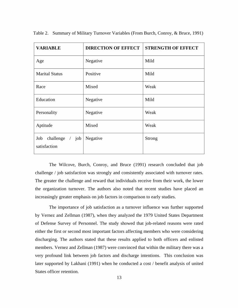
Table 2. Summary of Military Turnover Variables (From Burch, Conroy, & Bruce, 1991)


Age Negative Mild

Marital Status Positive Mild

Race Mixed Weak

Education Negative Mild

Personality Negative Weak

Aptitude Mixed Weak

Job challenge / job

satisfaction

Negative Strong

The Wilcove, Burch, Conroy, and Bruce (1991) research concluded that job

challenge / job satisfaction was strongly and consistently associated with turnover rates.

The greater the challenge and reward that individuals receive from their work, the lower

the organization turnover. The authors also noted that recent studies have placed an

increasingly greater emphasis on job factors in comparison to early studies.

The importance of job satisfaction as a turnover influence was further supported

by Vernez and Zellman (1987), when they analyzed the 1979 United States Department

of Defense Survey of Personnel. The study showed that job-related reasons were rated

either the first or second most important factors affecting members who were considering

discharging. The authors stated that these results applied to both officers and enlisted

members. Vernez and Zellman (1987) were convinced that within the military there was a

very profound link between job factors and discharge intentions. This conclusion was

later supported by Lakhani (1991) when he conducted a cost / benefit analysis of united

States officer retention.

14

Measures of intelligence or aptitude have been studied quite extensively in the

civilian community, but they have received very limited attention within the military

environment. The studies that have been conducted on military personal have focused

mainly on enlisted members. A study by Githens, Neumann, and Abrahams (1966) found

no correlation between the length of service of United States Naval officers and their

scores on the Naval College Aptitude test or the Officer Classification Battery scores.

A unique variable within the military turnover dynamic is the issue of mental

strength or mental toughness. Employment within the military is physically and mentally

more demanding than most civilian jobs. According to authors such as Cigrang, Todd,

Fielder, and Carbone (1999), psychological stamina needs to be considered when

analyzing turnover rates. These authors stress the importance of mental health during the

initial periods of training. The transition from civilian to military culture can be

accomplished only through intense training programs that place new recruits in

demanding situations that exceed their previous mental and physical limits.

A key concept in the analysis of military turnover is the Annualized Cost of

Leaving Model (ACOL). Warner and Goldberg developed this model in 1984 to predict

the effect of pay on separation rates. The model compares an individual’s cost of leaving

the military to the expected utility or reward they will derive from civilian employment.

The model has been used extensively by the Department of Defense to evaluate alternate

compensation strategies and their effect on employee turnover rates.

When the ACOL model was first developed, it was mainly used to assess enlisted

personnel. Smoker (1984) refined the ACOL model to estimate the effects on both

officers and enlisted personnel. The results that he obtained showed that the estimated

ACOL coefficient is closely linked to the assumed discount rate. The next step in

theoretical modeling was taken by Gotz and McCall (1984) when they developed the

Dynamic Retention Model (DRM). The DRM extends the Warner and Goldberg (1984)

model to officers’ career decisions. The DRM adds two additional elements to the ACOL

model: future uncertainty and taste for service. The DRM also considers the value an

15

officer may place on future career flexibility. The DRM can be used to explore different

policy options by taking individual retention decisions and running them through various

policy alternatives.

E. LITERATURE SUMMARY

The research literature clearly suggests that numerous factors help to predict

employee turnover, both military and civilian. The factors most commonly cited in the

literature include job satisfaction, pay, individual personal characteristics, promotion

opportunities, unemployment rate, and met expectations. The most consistent relationship

that emerged from both civilian and military research is that turnover is inversely

associated with job autonomy and job satisfaction. The more individuals feel empowered

and autonomous in their jobs, the higher their levels of job satisfaction and the higher

their propensity to remain with the organization. The literature provides a very good

indication of what variables should be included in a model that endeavors to quantify the

factors correlated with employee turnover.

16


17

III. REGRESSION ANALYSIS OF UNITED STATES MARINE CORPS OFFICERS

A. PURPOSE

The purpose of this chapter is to detail the United States Marine Corps (USMC)

officer commissioning system and to ascertain whether there is any correlation between

corps accession source allocation and retention. Firstly, the chapter will cover each of the

seven different accession sources to highlight the significant investment involved in

training USMC officers. Secondly, this chapter will develop regression models that

quantify the positive or negative impacts that USMC allocation has on retention.

B. COMMISSIONING PROGRAMS

There are seven different avenues through which a USMC officer can enlist; each

of these accession avenues is unique in terms of the potential candidate pool, the entry

requirements, and the length of training. The seven different commissioning sources are

as follows:

1. The United States Naval Academy (USNA)

Cadets who enter the USNA undertake a four-year training program that involves

both academic and military training. They graduate as an officer in either the Navy or the

USMC. To be eligible for consideration to attend the USNA, applicants must be United

States citizens, unmarried, have no dependants, be medically fit, and be at least 17, but no

older than 23, years of age. All USNA graduates are required to serve a minimum of five

years of active service.

2. Naval Reserve Officer Training Course (NROTC)

The NROTC is the second officer accession program that the Marine Corps runs

in conjunction with the Navy. The NROTC provides scholarship and non-scholarship

18

options at selected universities and colleges throughout the United States. In addition to

their academic training, NROTC midshipmen also receive extensive military training. To

be eligible for consideration, the NROTC applicants must be United States citizens,

medically fit, at least 17, but no older than 23 years, of age, and have no criminal record.

The minimum return of service obligation varies but is generally four years’ active

service.

3. Platoon Leaders Course (PLC)

The PLC program is open to all college students who are attending accredited

colleges and universities as full-time students. The program enables students to continue

with their studies, whilst also attending the Officer Candidate School (OCS). The training

at OCS consists of two six-week courses that are held during the summer holidays. The

minimum return of service obligation varies but is generally three years’ active and five

years’ reserve service.

4. Officer Candidate Course (OCC)

The OCC is a commissioning program that is open to college seniors or graduates.

It provides prospective USMC officers with a glimpse of Marine Corps life with

absolutely no commitment. Entry into the OCC begins with a ten-week course at OCS. If

candidates pass this ten-week course, they can choose to receive a reserve commission

and go to The Basic School (TBS) for additional training. The minimum return of service

obligation is generally three years’ active service and five years’ reserve service.

5. Marine Corps Enlisted Commissioning Program (MECEP)

The MECEP is designed to provide enlisted active duty Marines with the

opportunity to earn a college degree and become a USMC officer. Applicants must have

a minimum of six years’ active service and have attained the rank of Corporal or above.

If accepted into the program, the applicant attends a college with an NROTC unit on

campus. The minimum return of service obligation is four years’ active service.

19

6. Enlisted Commissioning Program (ECP)

The ECP allows qualified Marines to apply for assignment to Officer Cadet

School (OCS). To be eligible to apply for the program, Marines must have at least a

bachelor’s degree and be between 21 and 30 years of age. Upon graduation from OCS,

officers must serve a minimum of four years of active service and four years’ reserve

service.

7. Meritorious Commissioning Program (MCP)

The MCP ensures that Marines who do not have a bachelor’s-level degree still

have an avenue for commissioning as a USMC officer. This program gives Commanding

Officers the ability to nominate highly qualified enlisted Marines who have displayed

exceptional leadership. If accepted into the program, Marines attend the 10-week course

at OCS. The minimum return of service obligation is four years of active service and four

years’ reserve service.

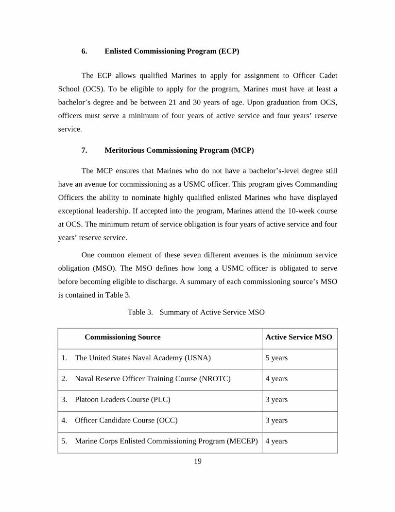
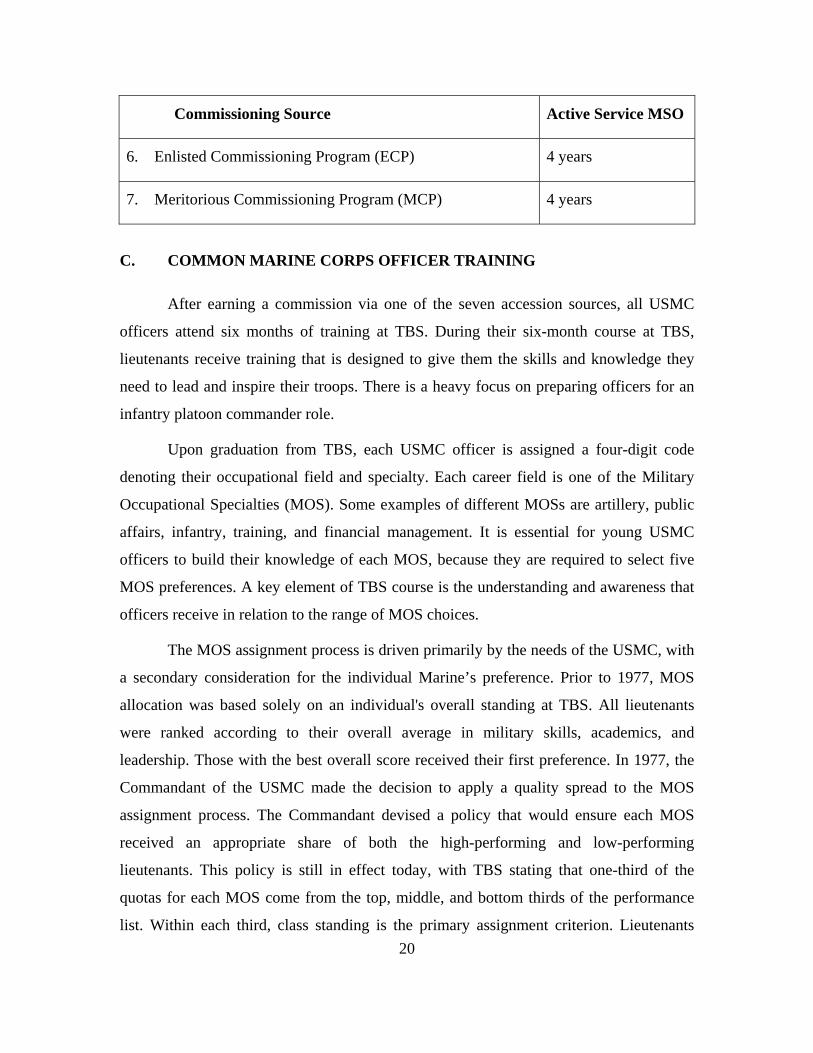
One common element of these seven different avenues is the minimum service

obligation (MSO). The MSO defines how long a USMC officer is obligated to serve

before becoming eligible to discharge. A summary of each commissioning source’s MSO

is contained in Table 3.

Table 3. Summary of Active Service MSO

Commissioning Source Active Service MSO

1. The United States Naval Academy (USNA) 5 years

2. Naval Reserve Officer Training Course (NROTC) 4 years

3. Platoon Leaders Course (PLC) 3 years

4. Officer Candidate Course (OCC) 3 years

5. Marine Corps Enlisted Commissioning Program (MECEP) 4 years

20

Commissioning Source Active Service MSO

6. Enlisted Commissioning Program (ECP) 4 years

7. Meritorious Commissioning Program (MCP) 4 years

C. COMMON MARINE CORPS OFFICER TRAINING

After earning a commission via one of the seven accession sources, all USMC

officers attend six months of training at TBS. During their six-month course at TBS,

lieutenants receive training that is designed to give them the skills and knowledge they

need to lead and inspire their troops. There is a heavy focus on preparing officers for an

infantry platoon commander role.

Upon graduation from TBS, each USMC officer is assigned a four-digit code

denoting their occupational field and specialty. Each career field is one of the Military

Occupational Specialties (MOS). Some examples of different MOSs are artillery, public

affairs, infantry, training, and financial management. It is essential for young USMC

officers to build their knowledge of each MOS, because they are required to select five

MOS preferences. A key element of TBS course is the understanding and awareness that

officers receive in relation to the range of MOS choices.

The MOS assignment process is driven primarily by the needs of the USMC, with

a secondary consideration for the individual Marine’s preference. Prior to 1977, MOS

allocation was based solely on an individual's overall standing at TBS. All lieutenants

were ranked according to their overall average in military skills, academics, and

leadership. Those with the best overall score received their first preference. In 1977, the

Commandant of the USMC made the decision to apply a quality spread to the MOS

assignment process. The Commandant devised a policy that would ensure each MOS

received an appropriate share of both the high-performing and low-performing

lieutenants. This policy is still in effect today, with TBS stating that one-third of the

quotas for each MOS come from the top, middle, and bottom thirds of the performance

list. Within each third, class standing is the primary assignment criterion. Lieutenants

21

near the top of their one-third have the best opportunity to receive one of their top

choices. Lieutenants near the bottom of their one-third increment have a lesser chance.

D. DATA AND VARIABLES

To ascertain whether there is any correlation between Corps allocation and

retention required capturing a large amount of data. Unfortunately this data was not

available from one central agency. To enable robust regression analysis, data was secured

from two separate agencies and then merged into one data set. The two agencies that

supplied data for this thesis were the Center for Naval Analyses (CNA) and the Total

Force Data Warehouse (TFDW).

1. Center for Naval Analyses (CNA)

The CNA is a non-profit institution that conducts high-level, in-depth research

and analysis to inform and shape the work of public sector decision makers. The CNA is

a federally funded research and development center serving the Department of the Navy

and other defense agencies. The CNA is responsible for collecting and storing a vast

amount of Department of Defense (DoD) data. Included in the data maintained by CNA

is panel data for USMC officers. Each officer’s data file includes general demographic

information, TBS academic performance, commissioning source, the top three MOS

preferences, and the primary MOS.

2. Total Force Data Warehouse (TFDW)

The TFDW is the USMC knowledge management system that collects and

maintains information on all USMC officers and enlisted members. TFDW data files

were used to supplement the information that was obtained from CNA. Information that

was drawn from the TFDW file and merged into the CNA file included length of service,

commissioning sources, and pay levels (Blackman 2009).

A data extract from CNA and TFDW were merged, which resulted in 37,080 data

points. The data set contained information on USMC officers from 1980 to 2006. The

first step in refining the data was to remove fiscal years 1980 to 1993 and 2000. They

22

were removed because no MOS preference information was maintained during these

years. The next step was to remove fiscal years 2003 to 2006, because officers were still

bound by a return of service obligation during this period. The end result was a final

sample size including data for 6,114 USMC officers.

E. REGRESSION ANALYSIS

This research utilizes a computer program called Stata to run regressions on the

USMC data. Stata is an integrated statistical package that enables data analysis and data

management. The full range of data that was inputted into Stata included a wide range of

demographic and service characteristics for each officer. A full list of each variable and

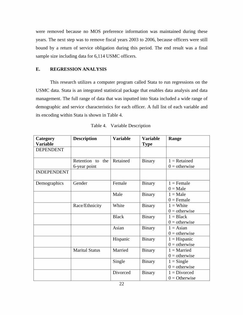
its encoding within Stata is shown in Table 4.

Table 4. Variable Description

Category Variable

Description Variable Variable Type

Range

DEPENDENT

Retention to the 6-year point

Retained Binary 1 = Retained 0 = otherwise

INDEPENDENT

Demographics Gender Female Binary 1 = Female 0 = Male

Male Binary 1 = Male 0 = Female

Race/Ethnicity White Binary 1 = White 0 = otherwise

Black Binary 1 = Black 0 = otherwise

Asian Binary 1 = Asian 0 = otherwise

Hispanic Binary 1 = Hispanic 0 = otherwise

Marital Status Married Binary 1 = Married 0 = otherwise

Single Binary 1 = Single 0 = otherwise

Divorced Binary 1 = Divorced 0 = Otherwise

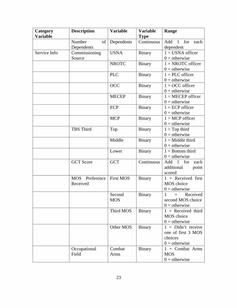
23

Category Variable


Range

Number of Dependents

Dependents Continuous Add 1 for each dependent

Service Info Commissioning Source

USNA Binary 1 = USNA officer 0 = otherwise

NROTC Binary 1 = NROTC officer 0 = otherwise

PLC Binary 1 = PLC officer 0 = otherwise

OCC Binary 1 = OCC officer 0 = otherwise

MECEP Binary 1 = MECEP officer 0 = otherwise

ECP Binary 1 = ECP officer 0 = otherwise

MCP Binary 1 = MCP officer 0 = otherwise

TBS Third Top Binary 1 = Top third 0 = otherwise

Middle Binary 1 = Middle third 0 = otherwise

Lower Binary 1 = Bottom third 0 = otherwise

GCT Score GCT Continuous Add 1 for each additional point scored

MOS Preference Received

First MOS Binary 1 = Received first MOS choice 0 = otherwise

Second MOS

Binary 1 = Received second MOS choice 0 = otherwise

Third MOS Binary 1 = Received third MOS choice 0 = otherwise

Other MOS Binary 1 = Didn’t receive one of first 3 MOS choices 0 = otherwise

Occupational Field

Combat Arms

Binary 1 = Combat Arms MOS 0 = otherwise

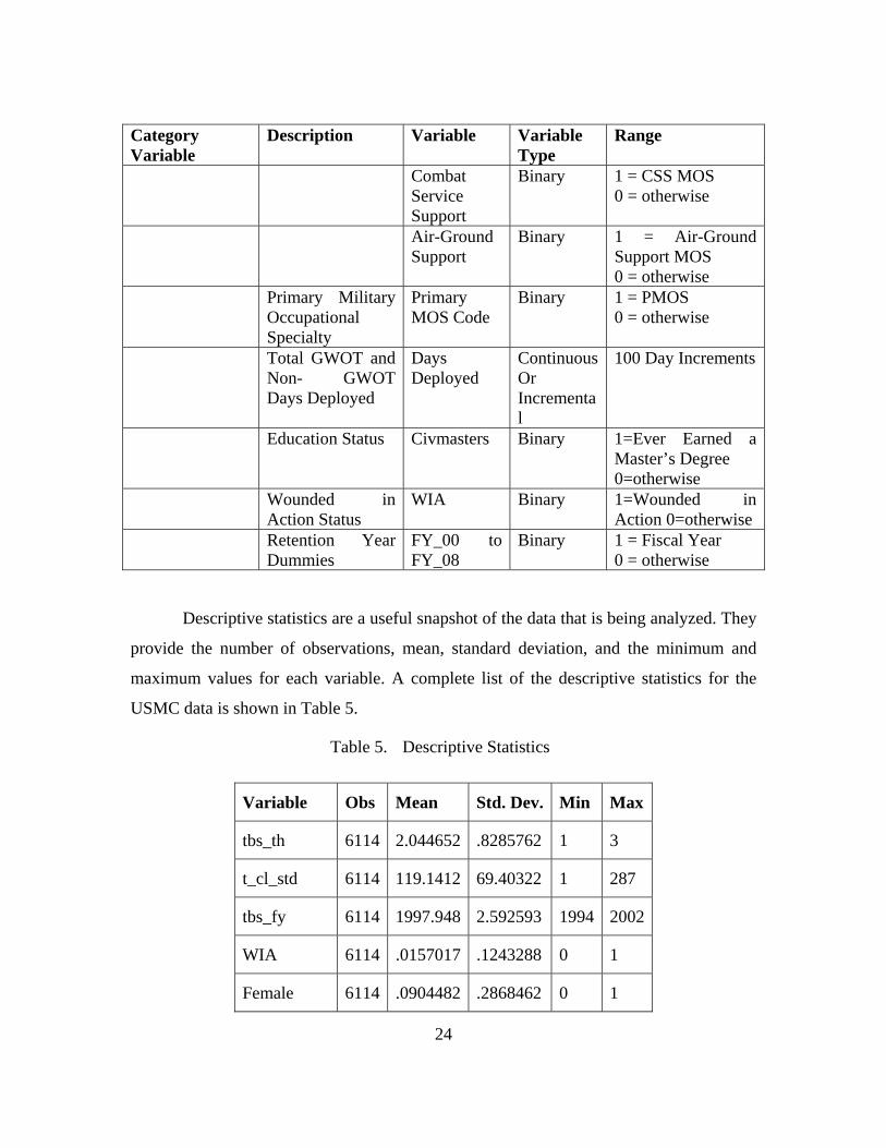
24

Category Variable


Range

Combat Service Support

Binary 1 = CSS MOS 0 = otherwise

Air-Ground Support

Binary 1 = Air-Ground Support MOS 0 = otherwise

Primary Military Occupational Specialty

Primary MOS Code

Binary 1 = PMOS 0 = otherwise

Total GWOT and Non- GWOT Days Deployed

Days Deployed

Continuous Or Incremental

100 Day Increments

Education Status Civmasters Binary 1=Ever Earned a Master’s Degree 0=otherwise

Wounded in Action Status

WIA Binary 1=Wounded in Action 0=otherwise

Retention Year Dummies

FY_00 to FY_08

Binary 1 = Fiscal Year 0 = otherwise

Descriptive statistics are a useful snapshot of the data that is being analyzed. They

provide the number of observations, mean, standard deviation, and the minimum and

maximum values for each variable. A complete list of the descriptive statistics for the

USMC data is shown in Table 5.

Table 5. Descriptive Statistics

Variable Obs Mean Std. Dev. Min Max

tbs_th 6114 2.044652 .8285762 1 3

t_cl_std 6114 119.1412 69.40322 1 287

tbs_fy 6114 1997.948 2.592593 1994 2002

WIA 6114 .0157017 .1243288 0 1

Female 6114 .0904482 .2868462 0 1

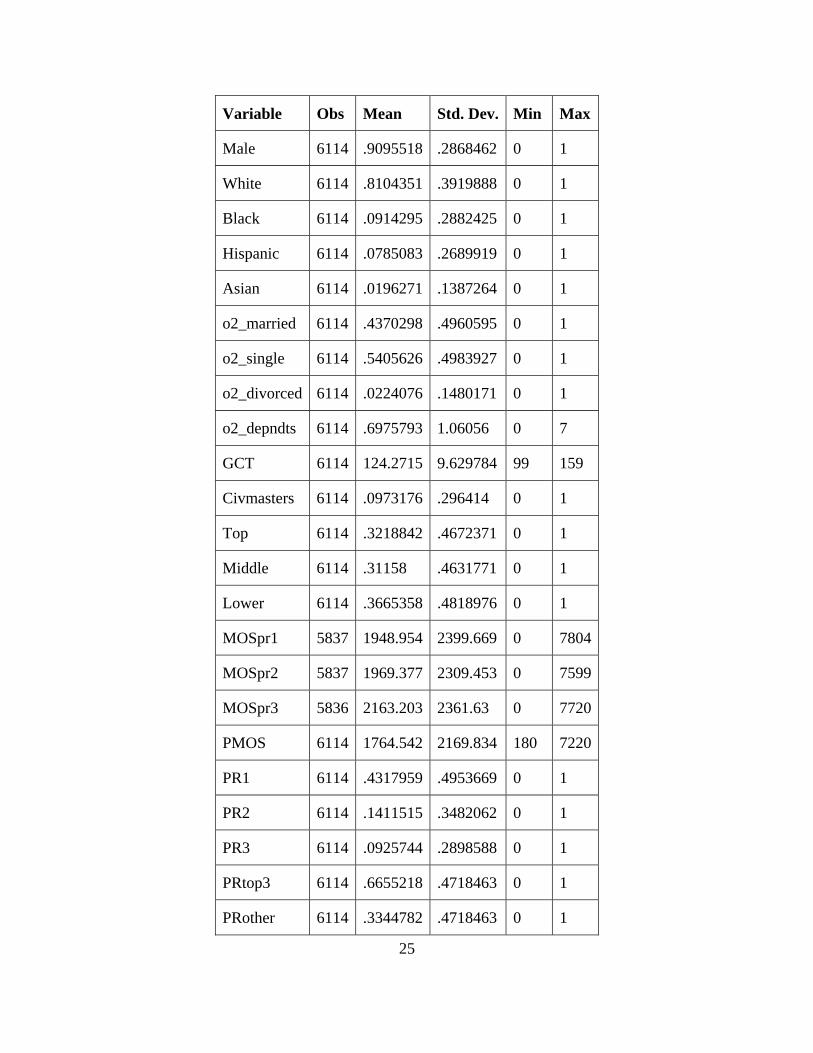
25


Male 6114 .9095518 .2868462 0 1

White 6114 .8104351 .3919888 0 1

Black 6114 .0914295 .2882425 0 1

Hispanic 6114 .0785083 .2689919 0 1

Asian 6114 .0196271 .1387264 0 1

o2_married 6114 .4370298 .4960595 0 1

o2_single 6114 .5405626 .4983927 0 1

o2_divorced 6114 .0224076 .1480171 0 1

o2_depndts 6114 .6975793 1.06056 0 7

GCT 6114 124.2715 9.629784 99 159

Civmasters 6114 .0973176 .296414 0 1

Top 6114 .3218842 .4672371 0 1

Middle 6114 .31158 .4631771 0 1

Lower 6114 .3665358 .4818976 0 1

MOSpr1 5837 1948.954 2399.669 0 7804

MOSpr2 5837 1969.377 2309.453 0 7599

MOSpr3 5836 2163.203 2361.63 0 7720

PMOS 6114 1764.542 2169.834 180 7220

PR1 6114 .4317959 .4953669 0 1

PR2 6114 .1411515 .3482062 0 1

PR3 6114 .0925744 .2898588 0 1

PRtop3 6114 .6655218 .4718463 0 1

PRother 6114 .3344782 .4718463 0 1

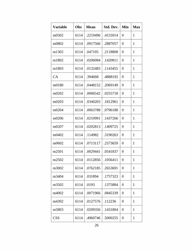
26


m0302 6114 .2219496 .4155914 0 1

m0802 6114 .0917566 .2887057 0 1

m1302 6114 .047105 .2118808 0 1

m1802 6114 .0206084 .1420811 0 1

m1803 6114 .0132483 .1143455 0 1

CA 6114 .394668 .4888192 0 1

m0180 6114 .0448152 .2069149 0 1

m0202 6114 .0006542 .0255718 0 1

m0203 6114 .0340203 .1812961 0 1

m0204 6114 .0063788 .0796188 0 1

m0206 6114 .0210991 .1437266 0 1

m0207 6114 .0202813 .1409725 0 1

m0402 6114 .114982 .3190263 0 1

m0602 6114 .0713117 .2573659 0 1

m2501 6114 .0029441 .0541837 0 1

m2502 6114 .0112856 .1056411 0 1

m3002 6114 .0762185 .2653691 0 1

m3404 6114 .031894 .1757323 0 1

m3502 6114 .0193 .1375884 0 1

m4002 6114 .0071966 .0845339 0 1

m4302 6114 .0127576 .112236 0 1

m5803 6114 .0209356 .1431804 0 1

CSS 6114 .4960746 .5000255 0 1

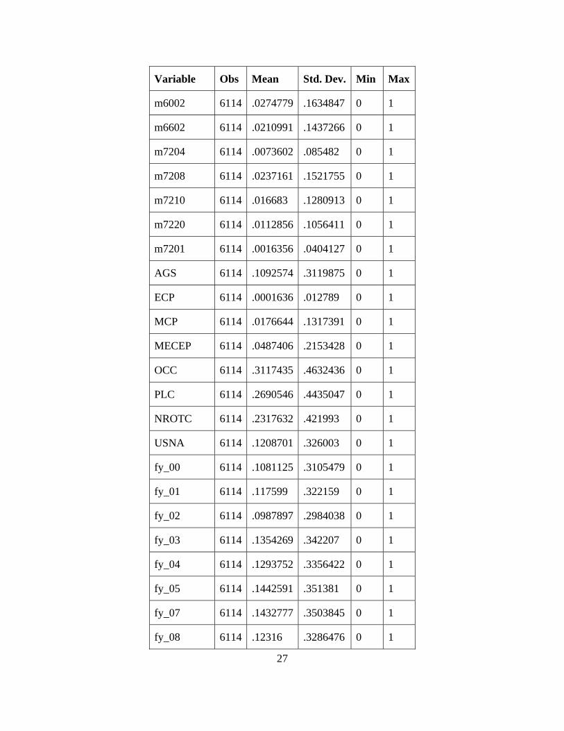
27


m6002 6114 .0274779 .1634847 0 1

m6602 6114 .0210991 .1437266 0 1

m7204 6114 .0073602 .085482 0 1

m7208 6114 .0237161 .1521755 0 1

m7210 6114 .016683 .1280913 0 1

m7220 6114 .0112856 .1056411 0 1

m7201 6114 .0016356 .0404127 0 1

AGS 6114 .1092574 .3119875 0 1

ECP 6114 .0001636 .012789 0 1

MCP 6114 .0176644 .1317391 0 1

MECEP 6114 .0487406 .2153428 0 1

OCC 6114 .3117435 .4632436 0 1

PLC 6114 .2690546 .4435047 0 1

NROTC 6114 .2317632 .421993 0 1

USNA 6114 .1208701 .326003 0 1

fy_00 6114 .1081125 .3105479 0 1

fy_01 6114 .117599 .322159 0 1

fy_02 6114 .0987897 .2984038 0 1

fy_03 6114 .1354269 .342207 0 1

fy_04 6114 .1293752 .3356422 0 1

fy_05 6114 .1442591 .351381 0 1

fy_07 6114 .1432777 .3503845 0 1

fy_08 6114 .12316 .3286476 0 1

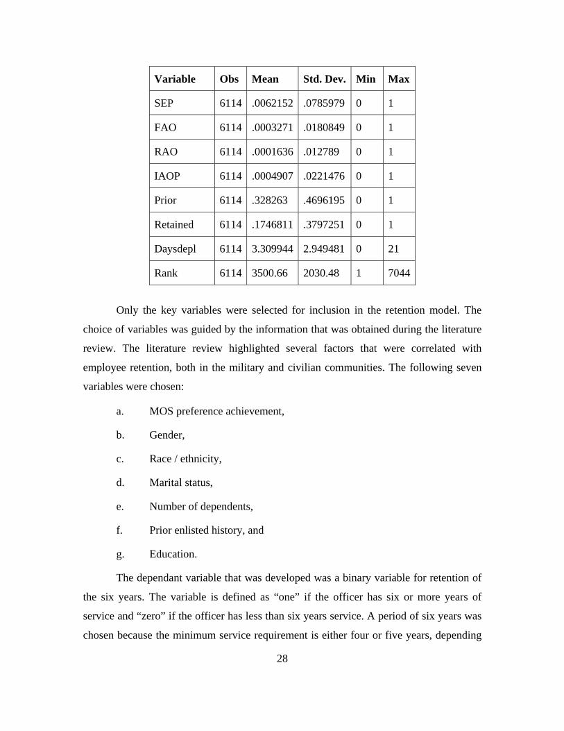
28


SEP 6114 .0062152 .0785979 0 1

FAO 6114 .0003271 .0180849 0 1

RAO 6114 .0001636 .012789 0 1

IAOP 6114 .0004907 .0221476 0 1

Prior 6114 .328263 .4696195 0 1

Retained 6114 .1746811 .3797251 0 1

Daysdepl 6114 3.309944 2.949481 0 21

Rank 6114 3500.66 2030.48 1 7044

Only the key variables were selected for inclusion in the retention model. The

choice of variables was guided by the information that was obtained during the literature

review. The literature review highlighted several factors that were correlated with

employee retention, both in the military and civilian communities. The following seven

variables were chosen:

a. MOS preference achievement,

b. Gender,

c. Race / ethnicity,

d. Marital status,

e. Number of dependents,

f. Prior enlisted history, and

g. Education.

The dependant variable that was developed was a binary variable for retention of

the six years. The variable is defined as “one” if the officer has six or more years of

service and “zero” if the officer has less than six years service. A period of six years was

chosen because the minimum service requirement is either four or five years, depending

29

on commissioning source. A six-year dependant variable allows for the variance in

operational requirements, individual circumstances, and service extensions.

The model that was developed was a simple linear probability model (a multiple

linear regression model with a binary dependant variable). It can be expressed in the

following manner:

Retained 6 years = β1*MOS first Preference Achievement + β2*MOS

second Preference Achievement + β3*MOS Preference Achievement not

in top 3 + β4*White + β5*Black + β6*Hispanic + β7*Married +

β8*Number of Dependents + β9*Prior Enlisted + β7*Education (civilian

masters) + β8*FY dummy variables + u

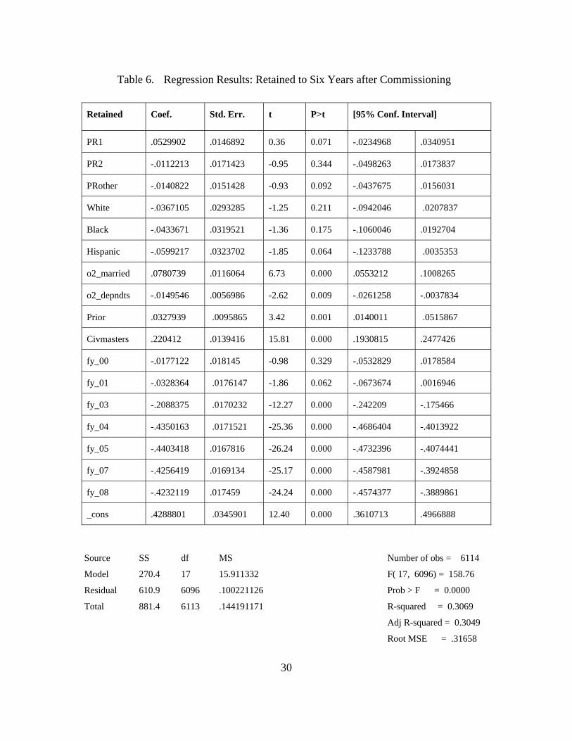
When the model was run in Stata, the results showed that there are significant

differences between the retention dynamics of USMC officers who receive their first

MOS preference and those who were allocated to an MOS that was outside of their top

three choices. The independent variable for first MOS preference is positive and

significant at a 10% level of significance; the coefficient for receiving first MOS is

0.05299. The independent variable for second MOS preference is slightly negative with a

coefficient of -0.01122. The independent variable for other MOS preferences (outside the

top three) is negative and significant at a 10% level of significance; the coefficient for

receiving other MOS preference is -0.01408.

The results from the regression analysis show the overall goodness-of-fit of the

model is reasonable as the R-squared value is 0.31. An R-squared value of 0.31 means

that for the USMC officers who remained serving until the six year mark, 31% of the

reason why they remained is explained by the variables contained in the model. This

result is quite strong when consideration is given to the wide range of factors that shape

retention. A full summary of the regression results from Stata are contained in Table 6.

30

Table 6. Regression Results: Retained to Six Years after Commissioning

Retained Coef. Std. Err. t P>t [95% Conf. Interval]

PR1 .0529902 .0146892 0.36 0.071 -.0234968 .0340951

PR2 -.0112213 .0171423 -0.95 0.344 -.0498263 .0173837

PRother -.0140822 .0151428 -0.93 0.092 -.0437675 .0156031

White -.0367105 .0293285 -1.25 0.211 -.0942046 .0207837

Black -.0433671 .0319521 -1.36 0.175 -.1060046 .0192704

Hispanic -.0599217 .0323702 -1.85 0.064 -.1233788 .0035353

o2_married .0780739 .0116064 6.73 0.000 .0553212 .1008265

o2_depndts -.0149546 .0056986 -2.62 0.009 -.0261258 -.0037834

Prior .0327939 .0095865 3.42 0.001 .0140011 .0515867

Civmasters .220412 .0139416 15.81 0.000 .1930815 .2477426

fy_00 -.0177122 .018145 -0.98 0.329 -.0532829 .0178584

fy_01 -.0328364 .0176147 -1.86 0.062 -.0673674 .0016946

fy_03 -.2088375 .0170232 -12.27 0.000 -.242209 -.175466

fy_04 -.4350163 .0171521 -25.36 0.000 -.4686404 -.4013922

fy_05 -.4403418 .0167816 -26.24 0.000 -.4732396 -.4074441

fy_07 -.4256419 .0169134 -25.17 0.000 -.4587981 -.3924858

fy_08 -.4232119 .017459 -24.24 0.000 -.4574377 -.3889861

_cons .4288801 .0345901 12.40 0.000 .3610713 .4966888

Source SS df MS Number of obs = 6114

Model 270.4 17 15.911332 F( 17, 6096) = 158.76

Residual 610.9 6096 .100221126 Prob > F = 0.0000

Total 881.4 6113 .144191171 R-squared = 0.3069

Adj R-squared = 0.3049

Root MSE = .31658

31

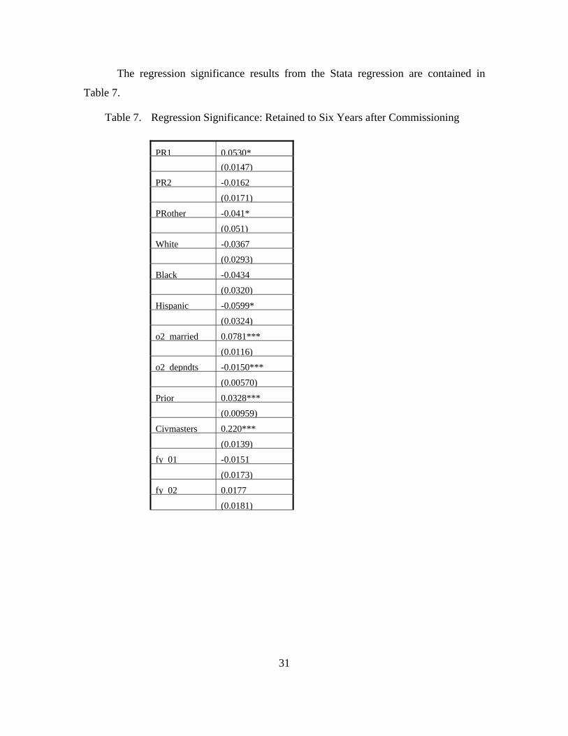
The regression significance results from the Stata regression are contained in

Table 7.

Table 7. Regression Significance: Retained to Six Years after Commissioning

PR1 0.0530*

(0.0147)

PR2 -0.0162

(0.0171)

PRother -0.041*

(0.051)

White -0.0367

(0.0293)

Black -0.0434

(0.0320)

Hispanic -0.0599*

(0.0324)

o2 married 0.0781***

(0.0116)

o2 depndts -0.0150***

(0.00570)

Prior 0.0328***

(0.00959)

Civmasters 0.220***

(0.0139)

fy 01 -0.0151

(0.0173)

fy 02 0.0177

(0.0181)

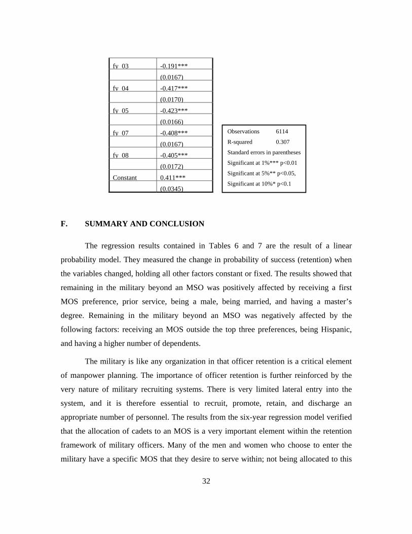
32

fy 03 -0.191***

(0.0167)

fy 04 -0.417***

(0.0170)

fy 05 -0.423***

(0.0166)

fy 07 -0.408***

(0.0167)

fy 08 -0.405***

(0.0172)

Constant 0.411***

(0.0345)

F. SUMMARY AND CONCLUSION

The regression results contained in Tables 6 and 7 are the result of a linear

probability model. They measured the change in probability of success (retention) when

the variables changed, holding all other factors constant or fixed. The results showed that

remaining in the military beyond an MSO was positively affected by receiving a first

MOS preference, prior service, being a male, being married, and having a master’s

degree. Remaining in the military beyond an MSO was negatively affected by the

following factors: receiving an MOS outside the top three preferences, being Hispanic,

and having a higher number of dependents.

The military is like any organization in that officer retention is a critical element

of manpower planning. The importance of officer retention is further reinforced by the

very nature of military recruiting systems. There is very limited lateral entry into the

system, and it is therefore essential to recruit, promote, retain, and discharge an

appropriate number of personnel. The results from the six-year regression model verified

that the allocation of cadets to an MOS is a very important element within the retention

framework of military officers. Many of the men and women who choose to enter the

military have a specific MOS that they desire to serve within; not being allocated to this

Observations 6114

R-squared 0.307

Standard errors in parentheses

Significant at 1%*** p<0.01

Significant at 5%** p<0.05,

Significant at 10%* p<0.1

33

MOS can be a shattering experience. Failing to secure a high MOS preference

significantly and negatively impacts retention beyond an officer’s minimum service

obligation. It is essential that officer accession sources maximize the number of cadets

who receive a high-order MOS preference.

34


35

IV. ROYAL MILITARY COLLEGE MODELING ANALYSIS

A. SCOPE

The purpose of this chapter is to define the Australian Army corps allocation

process and to develop models that optimize both organizational and individual

outcomes. Firstly, the chapter will cover the Corps’ allocation process that currently

occurs at the Royal Military College Duntroon (RMC). Secondly, this chapter will

develop models that will allow RMC staff to detail weighting for specific variables whilst

also maximizing the percentage of staff cadets (cadets) receiving their first or second

corps preference.

The cost of training each cadet to become a junior officer in the Australian Army

is extremely high. It is imperative every effort is made to provide each cadet with a

rewarding career in their chosen field. The first step in this process is achieving a corps

allocation that maximizes the cadet’s preferences whilst also meeting the requirements of

Army. Accurate models are needed to help the Australian Army develop corps allocation

processes that will retain a sufficient number of officers who have the right qualities.

B. BACKGROUND

In 1974, the decision was made that all initial Army officer training would be

centralized at RMC. Accordingly, in 1986, RMC took over the training responsibilities

from all other full-time Army officer training establishments, including the Officer Cadet

School at Portsea, Victoria; the Women’s Officer Training Wing at Georges Heights,

Sydney, New South Wales; and the Specialist Officer training wing at Canungra,

Queensland. Beginning in 1986, RMC has provided a course of between 12–18 months in

duration. Upon graduation from RMC, cadets are commissioned as lieutenants in the

Australian Army.

Generally, direct intakes occur every January and July, and all direct-entry cadets

undertake an 18-month training program. New officer candidates enlist as third-class

cadets and progress to second-class cadets after six months; they become first-class

36

cadets after 12 months. Graduates of the Australian Defence Force Academy (ADFA)

join at the beginning of each calendar year and are amalgamated with the new second-

class cadets. The RMC direct-entry cadets and ADFA graduates then spend their final 12

months of officer training together.

The charter of RMC is to prepare cadets and other selected candidates for careers

in the Army. Cadets are prepared for their careers via leadership training that promotes

integrity, high ideals, the pursuit of excellence, and a sense of duty, loyalty, and service

to the nation. The mission of RMC is to produce officers capable of commanding platoon

groups in the hardened and networked Army and to prepare specialist candidates for

commissioning. Toward the end of their time at RMC, each cadet nominates four corps in

which they would like to serve upon graduation. The cadets list the corps in order from

most desired to least desired.

The RMC structure includes the following elements:

Headquarters RMC—including the Commandant , Director of Military Art and the Director of Army Reserve Training;

Military Art and Training Wing;

Army Reserve Training Development Wing; and

Corps of Staff Cadets (which consists of the five cadet Companies).

C. CURRENT PROCESS

Allocating cadets to a specific corps is handled by the Corps Allocation Board

(CAB). The CAB is generally comprised of the following personnel: RMC staff,

Directorate of Officer Career Management (DOCM-A) staff, and members from the

Directorate of Personnel Army (DPERS-A). The purpose of the CAB is to assign cadets

to a specific corps fairly whilst adhering to the manning requirements. The process is

intended to give due regard to cadet preferences whilst adhering to the manning

requirements. The following factors are to be considered in relation to each cadet’s corps

allocation:

37

a. army manning requirements;

b. cadet preferences;

c. assessment of the person as a whole, including:

(1) officer qualities,

(2) academic performance,

(3) performance fit,

(4) participation,

(5) leadership and teamwork,

(6) conduct, and

(7) negative selection (i.e., CP33).

d. distribution of ability;

e. gender proportionality (where applicable), and

f. medical restrictions.

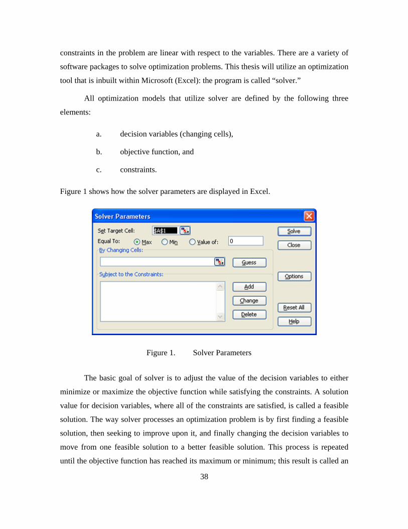
D. OPTIMIZATION MODELING

Optimization modeling is a type of mathematical modeling that attempts to

optimize (maximize or minimize) an objective function without violating resource

constraints. In essence, optimization modeling finds the answer that yields the best result,

given the specified constraints. It could be the answer that attains the highest profit,

output, or utility. Alternatively, it could be the answer that achieves the lowest cost,

waste, or minimizes losses. Optimization problems often involve making the most

efficient use of a finite resource. The resources could be money, time, machine hours,

labor, inventory, office space, or job functions. The range of optimization problems is as

wide as the range of techniques available to solve them. Optimization problems are often

classified as either linear or nonlinear, depending on whether the objectives and

3 Color blindness

38

constraints in the problem are linear with respect to the variables. There are a variety of

software packages to solve optimization problems. This thesis will utilize an optimization

tool that is inbuilt within Microsoft (Excel): the program is called “solver.”

All optimization models that utilize solver are defined by the following three

elements:

a. decision variables (changing cells),

b. objective function, and

c. constraints.

Figure 1 shows how the solver parameters are displayed in Excel.

Figure 1. Solver Parameters

The basic goal of solver is to adjust the value of the decision variables to either

minimize or maximize the objective function while satisfying the constraints. A solution

value for decision variables, where all of the constraints are satisfied, is called a feasible

solution. The way solver processes an optimization problem is by first finding a feasible

solution, then seeking to improve upon it, and finally changing the decision variables to

move from one feasible solution to a better feasible solution. This process is repeated

until the objective function has reached its maximum or minimum; this result is called an

39

optimal solution. For the objective function to describe the behavior of the measure of

effectiveness, it must capture the relationship between that measure and the decision

variables that cause it to change. A decision variable is a variable that can be directly

controlled by the decision maker.

1. Decision Variables

Decision variables are the cells on the Excel spreadsheet that the decision maker

can change or adjust to optimize the target cell. The cells in which these amounts are

recorded are the changing cells in this model. They usually measure the resources, such

as money, to be allocated to an activity. In this thesis, the decision variables are the

corps’ assignments for each individual cadet. Therefore, the total number of decision

variables equals the number of different corps available multiplied by the number of

cadets who need to be allocated to a corps. The decision variables are binary, assuming a

value of one if the cadet is assigned to that corps and zero otherwise. The vast number of

decision variables highlights the difficulty of the corps’ allocation process.

2. Objective Function

Once you have defined the decision variables, the next step is to define the

objective function. The objective function depends on the decision variables. In this

thesis, the objective function has been formulated as a maximizing cell that is increased

by higher cadet preference achievement.

3. Defining Constraints

In most models, constraints play a key role in determining what values the

decision variables can assume and what objective values can be attained. Constraints are

restrictions you place on the changing cells. To define a constraint, you first compute a

value based on the decision variables. Then, you place a limit (<=, = or >=) on this

computed value. In this thesis, the key constraint is the number of positions that are

available in each corps. Therefore, the constraint will be expressed as sum of decision

variables (cadets allocated to corps A) = the value of the constraint (number of positions

available with corps A).

40

Solver also allows you to specify that all decision variables are integers (whole

numbers). A particularly useful type of integer constraint specifies that a variable must

have an integer value with a lower bound of 0, and an upper bound of 1. This forces the

variable to be either 0 or 1, hence it can be used to model “yes / no” decisions. This type

of constraint was essential to this thesis as each decision variable needed to be an integer,

either a cadet was allocated to corps A or they were not allocated to corps A.

4. Interpreting Solver Solutions

A solution or set of values for the decision variables in which all of the constraints

in the Solver model are satisfied is called a “feasible solution.” Solver attempts to firstly

find a feasible solution and then improve it by finding another feasible solution that

increases (or decreases) the value of the objective function. An optimal solution is a

feasible solution wherein the objective function reaches a maximum (or minimum) value.

Data was obtained from RMC for cadets who graduated in 2008 and 2009. This

data contained a complete list of each cadet’s: corps preferences, actual allocation, and

Queens medal score. This data will be used to build models that maximize cadet

preferences whilst also meeting service requirements.

E. DATA

The benchmark data that the optimization models were compared against is actual

corps preferences and allocations from the 2008 and 2009 RMC graduating classes. The

only modification made to the data is to:

a. remove all foreign student (the do not receive a corps allocation), and

b. names have been replaced with numbers (to ensure privacy).

1. 2008 Data

Data was obtained from the RMC graduating class of 2008. Table 8 shows a

breakdown of each cadet's actual allocation, corps preferences and preference

achievement.

41

Table 8. Corps Preferences and Allocation (2008)

Name Actual First Pref Second Pref Third Pref Fourth Pref Pref achievement

1 AAAVN AAAVN AUSTINT RAAMC RACT 1

2 AAAVN AAAVN RAINF RAAC RAE 1

3 AAAVN AAAVN RAEME NIL NIL 1

4 AUSTINT AUSTINT RAAC RASIGS RAAMC 1

5 AUSTINT AUSTINT RACT RAAOC RAE 1

6 AUSTINT AUSTINT RAAC RACMP RAINF 1

7 AUSTINT AUSTINT RASIGS RACT RAEME 1

8 AUSTINT AUSTINT RAE RACT RASIGS 1

9 AUSTINT AUSTINT RAAC RACT RAAOC 1

10 AUSTINT AUSTINT RASIGS RAAMC RACT 1

11 AUSTINT AUSTINT RASIGS RAAMC RACT 1

12 RAA RAA RAEME RASIGS AAAVN 1

13 RAA RAA RAAC RAINF AUSTINT 1

14 RAA RAA RAEME RACT RACMP 1

15 RAA RAAMC RASIGS RAE AUSTINT 5

16 RAA RAAC RAA RASIGS RACT 2

17 RAA AUSTINT RAINF RAA RAAC 3

18 RAA RAA RAAC RASIGS RACT 1

19 RAA RAA RACMP RAINF RAEME 1

20 RAA RAINF RAE RASIGS RAA 4

21 RAA RACMP RACT RAA RASIGS 3

22 RAAC RAINF RAAC RAE RACT 2

23 RAAC RAAC AUSTINT RAE RACT 1

24 RAAC RAINF RAAC AUSTINT RAAMC 2

25 RAAC RAAC RAE RAINF RACT 1

26 RAAC RAINF RAAC RACMP AUSTINT 2

27 RAAC RAAC RAINF AUSTINT RAE 1

28 RAAC RAINF RAAC RAAOC RAE 2

29 RAAC RAAC RAINF RACT RAAOC 1

30 RAAMC RAAMC RASIGS RACT RACMP 1

31 RAAMC RAAMC RAINF RAAC AUSTINT 1

32 RAAOC RAE RASIGS RACT RAAOC 4

33 RAAOC RAAOC RACT RAAMC RAA 1

42


34 RAAOC RAAOC RACT RASIGS RAEME 1

35 RAAOC RAAOC RACT RACMP RASIGS 1

36 RAAOC RASIGS RAAOC RACT RACMP 2

37 RAAOC RAAOC RASIGS RAE RACMP 1

38 RAAOC AUSTINT RASIGS RACT N/A 5

39 RAAOC AUSTINT RAA RASIGS RAAC 5

40 RAAOC RACMP RAAOC RAE RASIGS 2

41 RAAOC RAAOC RACT RASIGS RAAMC 1

42 RACMP RACMP RACT RAAMC RAAOC 1

43 RACMP RACMP RACT RAAOC RAEME 1

44 RACMP RACMP RAE AUSTINT RAAC 1

45 RACMP RAINF RAAC RACMP RAE 3

46 RACT RACT RAE RAEME RAAOC 1

47 RACT RASIGS RACT RAAOC RAEME 2

48 RACT AUSTINT RACT RAE RASIGS 2

49 RACT RACT AUSTINT RAEME RAAOC 1

50 RACT RACT RASIGS RACMP RAAOC 1

51 RACT RAAC RACT RAE RASIGS 2

52 RACT RACT RAAMC RAAOC RACMP 1

53 RACT AUSTINT RASIGS RACT RAAOC 3

54 RACT RAAMC RACT RAAOC AUSTINT 2

55 RACT RACT RAAOC RACMP RASIGS 1

56 RAE RAINF RAE RAAC RACMP 2

57 RAE RAAC RAE RAINF RACMP 2

58 RAE RAE RAINF RASIGS RAAOC 1

59 RAE RAINF AUSTINT RAAC RAE 4

60 RAE RAE AUSTINT RAAC RASIGS 1

61 RAE RAE RACT RAAOC RASIGS 1

62 RAE RAE RAAC RAINF AUSTINT 1

63 RAE RAA RAE RASIGS RAAMC 2

64 RAEME RAINF RACT RAEME RASIGS 3

65 RAEME RAAC RASIGS RACT RAEME 4

66 RAEME RAEME RACC RAPC AUSTINT 1

67 RAEME RAEME RASIGS RAAOC RACT 1

68 RAEME AUSTINT RASIGS RACT RAEME 4

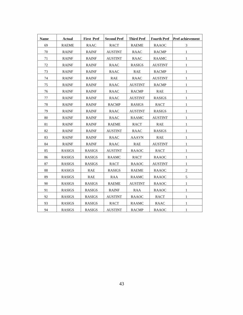
43


69 RAEME RAAC RACT RAEME RAAOC 3

70 RAINF RAINF AUSTINT RAAC RACMP 1

71 RAINF RAINF AUSTINT RAAC RAAMC 1

72 RAINF RAINF RAAC RASIGS AUSTINT 1

73 RAINF RAINF RAAC RAE RACMP 1

74 RAINF RAINF RAE RAAC AUSTINT 1

75 RAINF RAINF RAAC AUSTINT RACMP 1

76 RAINF RAINF RAAC RACMP RAE 1

77 RAINF RAINF RAAC AUSTINT RASIGS 1

78 RAINF RAINF RACMP RASIGS RACT 1

79 RAINF RAINF RAAC AUSTINT RASIGS 1

80 RAINF RAINF RAAC RAAMC AUSTINT 1

81 RAINF RAINF RAEME RACT RAE 1

82 RAINF RAINF AUSTINT RAAC RASIGS 1

83 RAINF RAINF RAAC AAAVN RAE 1

84 RAINF RAINF RAAC RAE AUSTINT 1

85 RASIGS RASIGS AUSTINT RAAOC RACT 1

86 RASIGS RASIGS RAAMC RACT RAAOC 1

87 RASIGS RASIGS RACT RAAOC AUSTINT 1

88 RASIGS RAE RASIGS RAEME RAAOC 2

89 RASIGS RAE RAA RAAMC RAAOC 5

90 RASIGS RASIGS RAEME AUSTINT RAAOC 1

91 RASIGS RASIGS RAINF RAA RAAOC 1

92 RASIGS RASIGS AUSTINT RAAOC RACT 1

93 RASIGS RASIGS RACT RAAMC RAAC 1

94 RASIGS RASIGS AUSTINT RACMP RAAOC 1

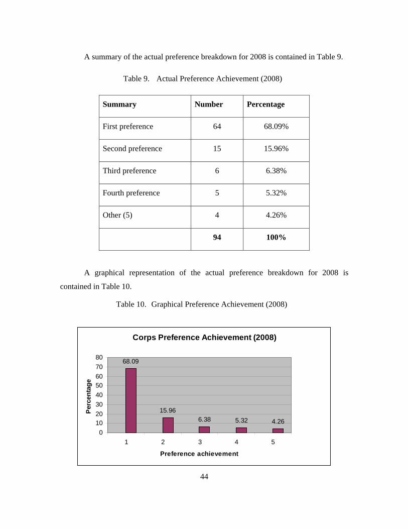
44

A summary of the actual preference breakdown for 2008 is contained in Table 9.

Table 9. Actual Preference Achievement (2008)

Summary Number Percentage

First preference 64 68.09%

Second preference 15 15.96%

Third preference 6 6.38%

Fourth preference 5 5.32%

Other (5) 4 4.26%

94 100%

A graphical representation of the actual preference breakdown for 2008 is

contained in Table 10.

Table 10. Graphical Preference Achievement (2008)

Corps Preference Achievement (2008)

68.09

15.966.38 5.32 4.26

0

1020

30

40

5060

70

80

1 2 3 4 5

Preference achievement

Per

cen

tag

e

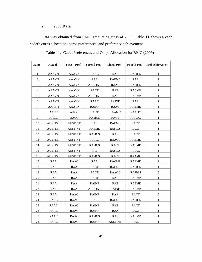
45

2. 2009 Data

Data was obtained from RMC graduating class of 2009. Table 11 shows a each

cadet's corps allocation, corps preferences, and preference achievement.

Table 11. Cadet Preferences and Corps Allocation for RMC (2009)


1 AAAVN AAAVN RAAC RAE RASIGS 1

2 AAAVN AAAVN RAE RAEME RAA 1

3 AAAVN AAAVN AUSTINT RAAC RASIGS 1

4 AAAVN AAAVN RACT RAE RACMP 1

5 AAAVN AAAVN AUSTINT RAE RACMP 1

6 AAAVN AAAVN RAAC RAINF RAA 1

7 AAAVN AAAVN RAINF RAAC RAEME 1

8 AACC AACC RACT RAAMC RAAOC 1

9 AACC AACC RASIGS RACT RAAOC 1

10 AUSTINT AUSTINT RAE RAEME RACT 1

11 AUSTINT AUSTINT RAEME RASIGS RACT 1

12 AUSTINT AUSTINT RASIGS RAE RACT 1

13 AUSTINT AUSTINT RAAC RAAOC RAEME 1

14 AUSTINT AUSTINT RASIGS RACT RAEME 1

15 AUSTINT AUSTINT RAE RASIGS RAAC 1

16 AUSTINT AUSTINT RASIGS RACT RAAMC 1

17 RAA RAAC RAA RACMP RAEME 2

18 RAA RAA RACT RAEME RASIGS 1

19 RAA RAA RACT RAAOC RASIGS 5

20 RAA RAA RACT RAE RACMP 1

21 RAA RAA RAINF RAE RAEME 1

22 RAA RAA AUSTINT RAINF RACMP 1

23 RAA RAAC RAINF RAA RACT 5

24 RAAC RAAC RAE RAEME RASIGS 1

25 RAAC RAAC RAINF RAE RACT 1

26 RAAC RAAC RAINF RAA RACT 1

27 RAAC RAAC RASIGS RAE RACMP 1

28 RAAC RAAC RAINF AUSTINT RAE 1

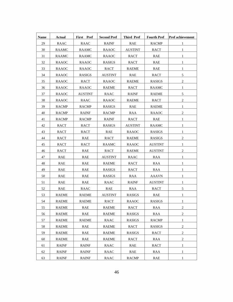
46


29 RAAC RAAC RAINF RAE RACMP 1

30 RAAMC RAAMC RAAOC AUSTINT RACT 1

31 RAAMC RAAMC RAAOC RACT RAE 1

32 RAAOC RAAOC RASIGS RACT RAE 1

33 RAAOC RAAOC RACT RAEME RAE 1

34 RAAOC RASIGS AUSTINT RAE RACT 5

35 RAAOC RACT RAAOC RAEME RASIGS 2

36 RAAOC RAAOC RAEME RACT RAAMC 1

37 RAAOC AUSTINT RAAC RAINF RAEME 5

38 RAAOC RAAC RAAOC RAEME RACT 2

39 RACMP RACMP RASIGS RAE RAEME 1

40 RACMP RAINF RACMP RAA RAAOC 2

41 RACMP RACMP RAINF RACT RAE 1

42 RACT RACT RASIGS AUSTINT RAAMC 1

43 RACT RACT RAE RAAOC RASIGS 1

44 RACT RAE RACT RAEME RASIGS 2

45 RACT RACT RAAMC RAAOC AUSTINT 1

46 RACT RAE RACT RAEME AUSTINT 2

47 RAE RAE AUSTINT RAAC RAA 1

48 RAE RAE RAEME RACT RAA 1

49 RAE RAE RASIGS RACT RAA 1

50 RAE RAE RASIGS RAA AAAVN 1

51 RAE RAE RAAC RAINF AUSTINT 1

52 RAE RAAC RAE RAA RACT 5

53 RAEME RAEME AUSTINT RASIGS RAE 1

54 RAEME RAEME RACT RAAOC RASIGS 1

55 RAEME RAE RAEME RACT RAA 2

56 RAEME RAE RAEME RASIGS RAA 2

57 RAEME RAEME RAAC RASIGS RACMP 1

58 RAEME RAE RAEME RACT RASIGS 2

59 RAEME RAE RAEME RASIGS RACT 2

60 RAEME RAE RAEME RACT RAA 2

61 RAINF RAINF RAAC RAE RACT 1

62 RAINF RAINF RAAC RAE RAA 1

63 RAINF RAINF RAAC RACMP RAE 1

47


64 RAINF RAINF RAAC AUSTINT RACMP 1

65 RAINF RAINF AUSTINT RACT RAE 1

66 RAINF RAINF RAAC RAE RAA 1

67 RAINF RAINF RAAOC RAA RAE 1

68 RAINF RAINF RAAC RAE RAAMC 1

69 RAINF RAINF RAAC RAE RACT 1

70 RAINF RAINF RAAC RAA RACT 1

71 RAINF RAINF AUSTINT RAAC RAE 1

72 RAINF RAINF RAAC RAA RACT 1

73 RAINF RAINF RAE RAEME RACT 1

74 RASIGS RASIGS AUSTINT RAINF RAAOC 1

75 RASIGS RASIGS AUSTINT RAINF RAEME 1

76 RASIGS AUSTINT RAA RASIGS RAEME 3

77 RASIGS RAA RASIGS RAEME RACT 2

78 RASIGS RASIGS RACMP RAA RAEME 1

79 RASIGS RAAMC RACT RASIGS RACMP 3

80 RASIGS RASIGS RAE RACT RAAOC 1

81 RASIGS AUSTINT RASIGS RAE RAEME 2

82 RASIGS RAE RASIGS RACT RAAOC 2

A summary of the actual preference breakdown for 2009 is contained in Table 12.

Table 12. Preference Achievement (2009)


First preferences 62 75.61%

Second preferences 15 18.29%

Third preferences 3 3.66%

Fourth preferences 0 0.00%

Other 2 2.44%

82 100.00%

48

A graphical representation of the actual preference achievement for 2009 is


Table 13. Graphical Preferences Achievement (2009)

Corps Preference Achievement (2009)

75.61

18.29

3.66 0 2.44

0

1020

30

40

5060

70

80

1 2 3 4 5

Preference achieved

Per

cen

tag

e

A summary of the actual preference achievement over the period 2008 / 2009 is


Table 14. Preference Achievement (2008 and 2009)




Third preferences 9 5.11%

Fourth preferences 5 2.84%

Other 6 3.41%

176 100.00%

49

A graphical representation of the actual preference achievement for 2008 / 2009 is


Table 15. Graphical Preferences Achievement (2008 /2009)

Corps Preference Achievement (2008 and 2009)

71.59

17.05

5.11 2.84 3.41

0

10

20

30

40

50

60

70

80

1 2 3 4 5

Preference Achieved

Per

cen

tag

e

F. MODEL ASSESSMENT

In order to effectively rank and assess optimization models, it is useful to define a

set of criteria that they will be assessed against. Chapter II concluded that the majority of

academics concur that recognition and reward of performance are important elements of

the retention dynamic. Therefore, “performance recognition” will be one of the factors

against which each model will be assessed. Chapter III developed a linear probability

model that utilized USMC data. The results showed that remaining in the military beyond

a minimum service obligation was positively affected by receiving your first Military

Occupational Specialties (MOS) preference, and was negatively affected by receiving a

lower order MOS preference. Therefore, “maximizing first preferences” and “minimizing

third, fourth and no preference” will both be categories that the models will be assessed

against. Each model will be given a score of either: high, medium or low in relation to

each of the three assessment categories. If a model performs well in relation to a category

it will receive a grading of high, and if it performs poorly it will be assessed a grading of

low.

50

G. MODEL 1 (WEIGHTED FOR CADET PREFERENCE)

The first optimization model that was developed utilized the number of positions

that were available and sought to maximize the number of cadets receiving an allocation

that was highest in their preferences. The inputs to the model were decision variables,

objective function, and constraints.

The decision variables were a function of the number of cadets that needed to be

allocated to a corps multiplied by the number of different corps that where available. For

the 2008 model, there were 12 possible corps available and 94 cadets who required an

allocation. The number of decision variables is a function of these two figures; therefore,

for the 2008 model there were 1,128 decision variables. For the 2009 model, there were

13 possible corps and 82 cadets; therefore, there were 1,066 decision variables. A sample

of the 2008 Model 1 decision variable is highlighted in Table 16.

Table 16. Decision Variables (Model 1)

CORPS

A B C D E F G H I J K

1 1 0 0 0 0 0 0 0 0 0 0

2 1 0 0 0 0 0 0 0 0 0 0

3 1 0 0 0 0 0 0 0 0 0 0

4 0 1 0 0 0 0 0 0 0 0 0

…..

C

A

D

E

T

94 0 0 0 0 0 0 0 0 0 0 1

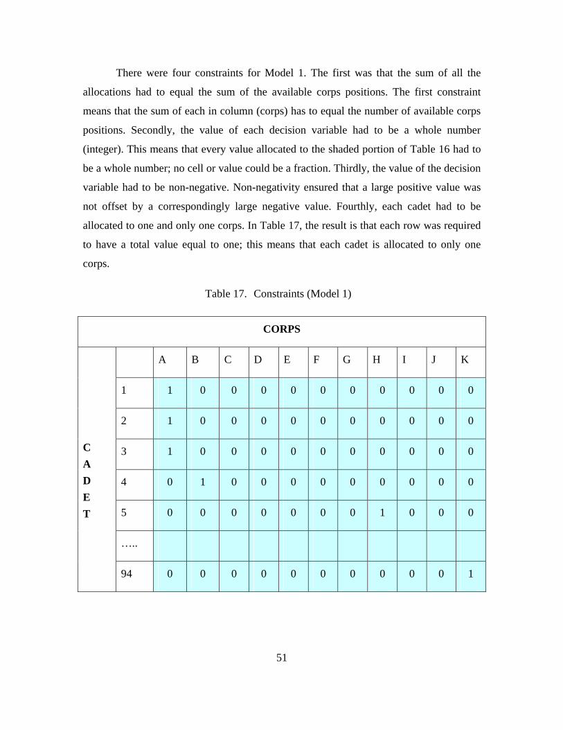
51

There were four constraints for Model 1. The first was that the sum of all the

allocations had to equal the sum of the available corps positions. The first constraint

means that the sum of each in column (corps) has to equal the number of available corps

positions. Secondly, the value of each decision variable had to be a whole number

(integer). This means that every value allocated to the shaded portion of Table 16 had to

be a whole number; no cell or value could be a fraction. Thirdly, the value of the decision

variable had to be non-negative. Non-negativity ensured that a large positive value was

not offset by a correspondingly large negative value. Fourthly, each cadet had to be

allocated to one and only one corps. In Table 17, the result is that each row was required

to have a total value equal to one; this means that each cadet is allocated to only one

corps.

Table 17. Constraints (Model 1)

CORPS

A B C D E F G H I J K

1 1 0 0 0 0 0 0 0 0 0 0

2 1 0 0 0 0 0 0 0 0 0 0

3 1 0 0 0 0 0 0 0 0 0 0

4 0 1 0 0 0 0 0 0 0 0 0

5 0 0 0 0 0 0 0 1 0 0 0

…..

C

A

D

E

T

94 0 0 0 0 0 0 0 0 0 0 1

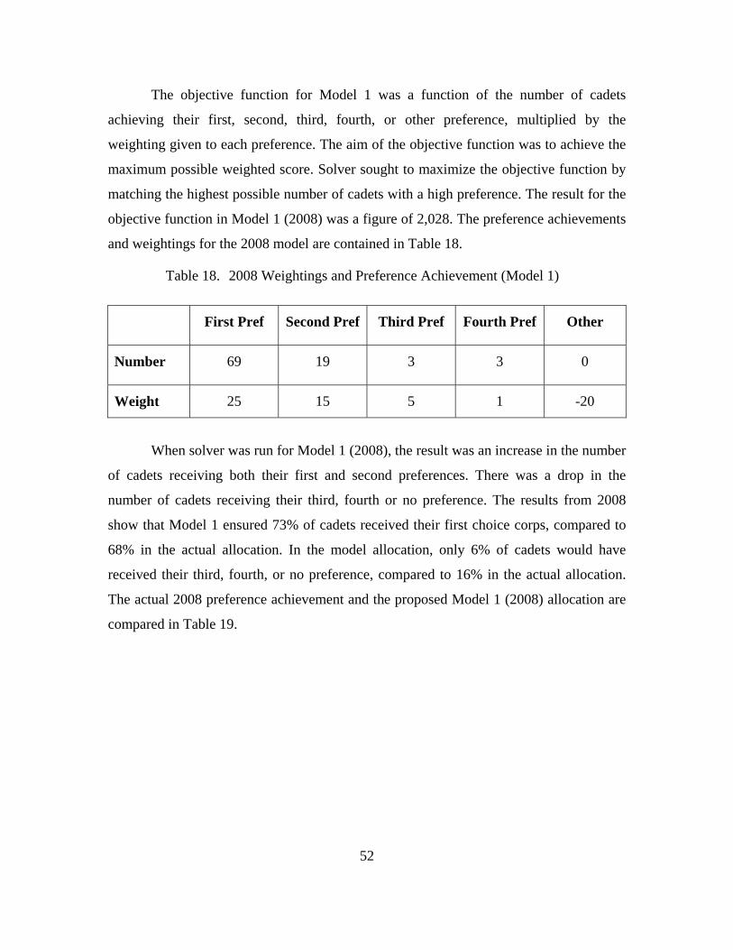
52

The objective function for Model 1 was a function of the number of cadets

achieving their first, second, third, fourth, or other preference, multiplied by the

weighting given to each preference. The aim of the objective function was to achieve the

maximum possible weighted score. Solver sought to maximize the objective function by

matching the highest possible number of cadets with a high preference. The result for the

objective function in Model 1 (2008) was a figure of 2,028. The preference achievements

and weightings for the 2008 model are contained in Table 18.

Table 18. 2008 Weightings and Preference Achievement (Model 1)

First Pref Second Pref Third Pref Fourth Pref Other

Number 69 19 3 3 0

Weight 25 15 5 1 -20

When solver was run for Model 1 (2008), the result was an increase in the number

of cadets receiving both their first and second preferences. There was a drop in the

number of cadets receiving their third, fourth or no preference. The results from 2008

show that Model 1 ensured 73% of cadets received their first choice corps, compared to

68% in the actual allocation. In the model allocation, only 6% of cadets would have

received their third, fourth, or no preference, compared to 16% in the actual allocation.

The actual 2008 preference achievement and the proposed Model 1 (2008) allocation are

compared in Table 19.

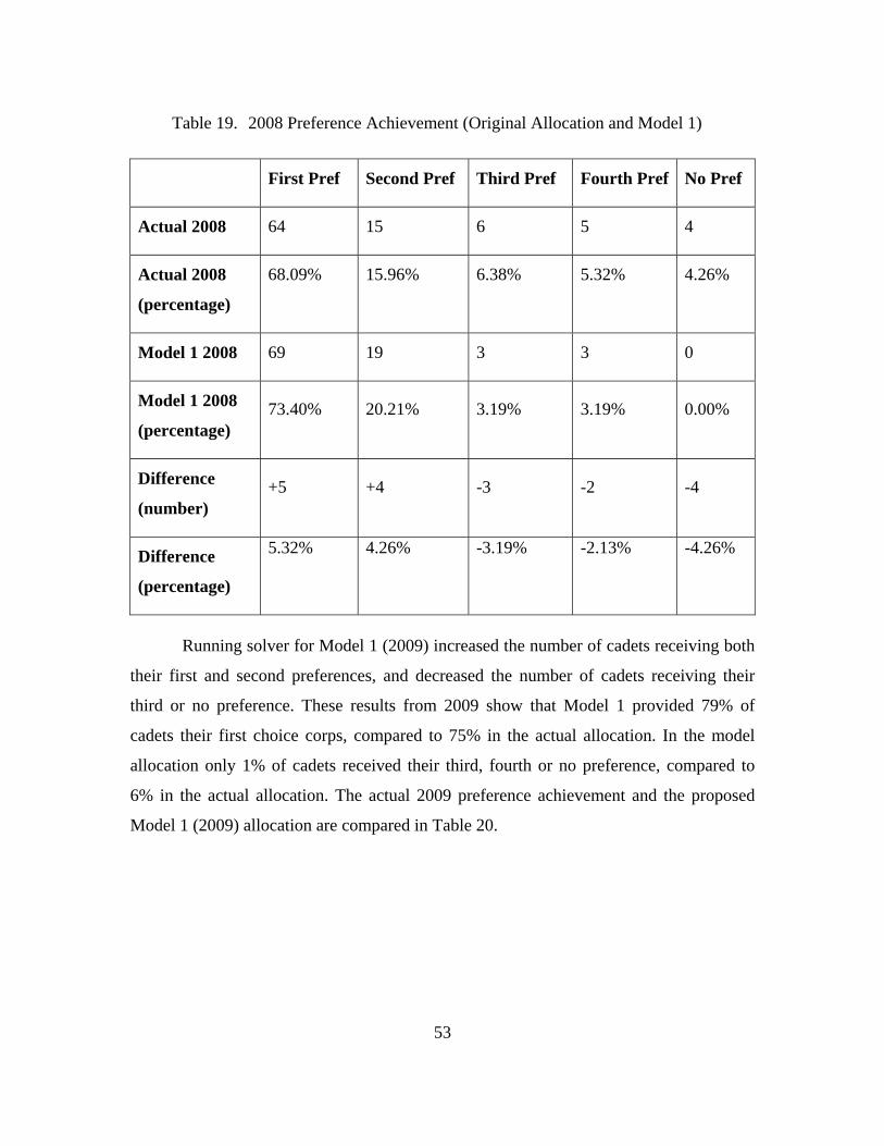
53

Table 19. 2008 Preference Achievement (Original Allocation and Model 1)

First Pref Second Pref Third Pref Fourth Pref No Pref

Actual 2008 64 15 6 5 4

Actual 2008

(percentage)

68.09% 15.96% 6.38% 5.32% 4.26%

Model 1 2008 69 19 3 3 0

Model 1 2008

(percentage) 73.40% 20.21% 3.19% 3.19% 0.00%

Difference

(number) +5 +4 -3 -2 -4

Difference

(percentage)

5.32% 4.26% -3.19% -2.13% -4.26%

Running solver for Model 1 (2009) increased the number of cadets receiving both

their first and second preferences, and decreased the number of cadets receiving their

third or no preference. These results from 2009 show that Model 1 provided 79% of

cadets their first choice corps, compared to 75% in the actual allocation. In the model

allocation only 1% of cadets received their third, fourth or no preference, compared to

6% in the actual allocation. The actual 2009 preference achievement and the proposed

Model 1 (2009) allocation are compared in Table 20.

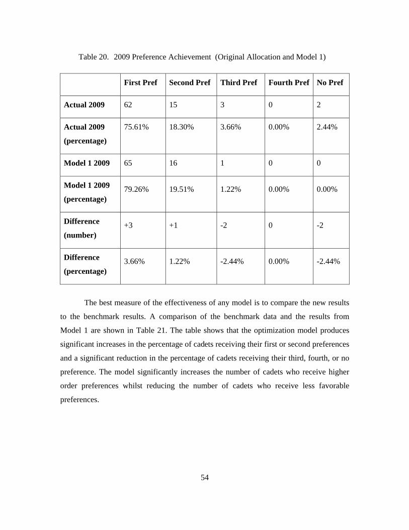
54



Actual 2009 62 15 3 0 2

Actual 2009

(percentage)

75.61% 18.30% 3.66% 0.00% 2.44%

Model 1 2009 65 16 1 0 0

Model 1 2009

(percentage) 79.26% 19.51% 1.22% 0.00% 0.00%

Difference

(number) +3 +1 -2 0 -2

Difference

(percentage) 3.66% 1.22% -2.44% 0.00% -2.44%

The best measure of the effectiveness of any model is to compare the new results

to the benchmark results. A comparison of the benchmark data and the results from

Model 1 are shown in Table 21. The table shows that the optimization model produces

significant increases in the percentage of cadets receiving their first or second preferences

and a significant reduction in the percentage of cadets receiving their third, fourth, or no

preference. The model significantly increases the number of cadets who receive higher

order preferences whilst reducing the number of cadets who receive less favorable

preferences.

55

Table 21. Model 1 Preference Achievement (2008 and 2009 Combined)


Actual

(number) 126 30 9 5 6

Actual

(percentage) 71.59% 17.05% 5.11% 2.84% 3.41%

Model 1

(number) 134 35 4 3 0

Model 1

(percentage) 76.14% 19.89% 2.27% 1.70% 0.00%

Difference

(number) 8 5 -5 -2 -6

Difference

(percentage) +4.55% +2.84% -2.84% -1.14% -3.41%

The results from Table 21 show that Model 1 provides a distinct improvement in

corps allocation that values cadet preferences. The performance of Model 1 in relation to

the three performance criteria is shown in Table 22.

56

Table 22. Model 1 Performance

Criteria Grade

Performance recognition Low

Maximizing first preferences High

Minimizing third, fourth and no preference High

Overall performance Medium

Model 1 does not take into account a cadet’s performance or Queens medal score

in allocating corps. The benefit of excluding performance as a driver for the allocation

process is that it aids in the even distribution of talent throughout each of the separate

corps. The militaries of many countries have actually developed policies that ensure each

of their corps is allocated an appropriate talent mix.

The USMC has a specific policy that ensures an even spread of talent and ability

throughout each of the Military Occupational Specialties (MOS). Every USMC lieutenant

is required to attend The Basic School (TBS) for a period of six months. At the end of

their training at TBS, all lieutenants are ranked according to their overall average in

military skills, academics, and leadership. TBS policy states that one-third of the quota

for each MOS comes from the top, middle, and bottom thirds of the performance list.

Within each third, class standing is the primary assignment criterion. Lieutenants near the

top of their one-third have the best opportunity to receive one of their top MOS choices.

Lieutenants near the bottom of their one-third increment have a smaller chance. This

policy ensures that each MOS receives an appropriate share of the higher performing and

lower performing lieutenants.

57

H. MODEL 2 (FIRST OR SECOND CHOICE CORPS GUARANTEE)

The second optimization model that was developed utilized the number of

positions that were available and ensured each cadet received an allocation that was

either their first or second corps preference. The inputs to the model were decision

variables, constraints, and objective function.


allocated to a corps multiplied by the number of different corps available. For the 2008

model, there were 12 possible corps and 94 cadets who required an allocation. The

number of decision variables is a function of these two figures; therefore, there were

1,128 decision variables for the 2008 model. For the 2009 model, there were 13 possible

corps and 82 cadets, yielding 1,066 decision variables.

There were four constraints for this model. The first was that the sum of all the

cadets achieving their first or second preference had to equal the total number of cadets

who required a corps allocation. Secondly, the value of each decision variable had to be a

whole number (integer). This means that every value allocated to the decision variable

matrix had to be a whole number; no cell or value could be a fraction. Thirdly, the value

of the decision variable had to be non-negative. Non-negativity ensured that a large

positive value was not offset by a correspondingly large negative value. Fourthly, each

cadet had to be allocated to a corps. This is evident in the decision variable matrix,

because each row is required to have a total value equal to one: having a value of one for

each row means that each cadet is allocated to one and only one corps.

The objective function for this model was to minimize the difference between the

positions available in each corps and the actual number of cadets allocated to each corps,

because it was not possible to assign all cadets to one of their top two choices and meet

the corps’ end-strength targets. Solver sought to minimize the objective function by

allocating every cadet to either their first or second corps preference, while also

minimizing the gap between the number of planned positions available for each corps and

the actual allocation to each corps.

58

When solver was run for Model 2 (2008), the result was an over-allocation in two

corps and a slight under-allocation in three corps. It is possible to ensure every cadet

achieves their first or second corps preference with minimal alteration to the planned

corps allocation numbers. A full list of the corps overages and underages is contained in

Table 23.

Table 23. Model 2 Corps Breakdown (2008)

A B C D E F G H I J K L M

Planned 3 n/a 8 10 8 2 10 4 10 8 6 15 10

Actual 3 n/a 8 9 8 5 8 4 10 8 4 17 10

Difference

(number) 0 n/a4 0 -1 0 +3 -2 0 0 0 -2 +2 0

For the 2008 data, Model 2 spreads cadets fairly evenly across their first or

second preference. A complete breakdown of the preference achievement is contained in

Table 24.

Table 24. Model 2 Preference Achievement (2008)




94 100.00%

4 Corps B was not available in 2008.

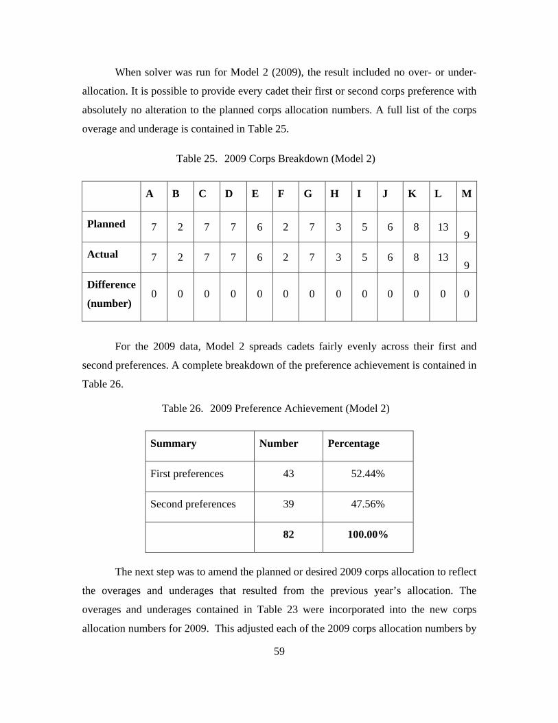
59

When solver was run for Model 2 (2009), the result included no over- or under-

allocation. It is possible to provide every cadet their first or second corps preference with

absolutely no alteration to the planned corps allocation numbers. A full list of the corps

overage and underage is contained in Table 25.

Table 25. 2009 Corps Breakdown (Model 2)


Planned 7 2 7 7 6 2 7 3 5 6 8 13 9

Actual 7 2 7 7 6 2 7 3 5 6 8 13 9

Difference

(number) 0 0 0 0 0 0 0 0 0 0 0 0 0

For the 2009 data, Model 2 spreads cadets fairly evenly across their first and

second preferences. A complete breakdown of the preference achievement is contained in

Table 26.

Table 26. 2009 Preference Achievement (Model 2)




82 100.00%

The next step was to amend the planned or desired 2009 corps allocation to reflect

the overages and underages that resulted from the previous year’s allocation. The

overages and underages contained in Table 23 were incorporated into the new corps

allocation numbers for 2009. This adjusted each of the 2009 corps allocation numbers by

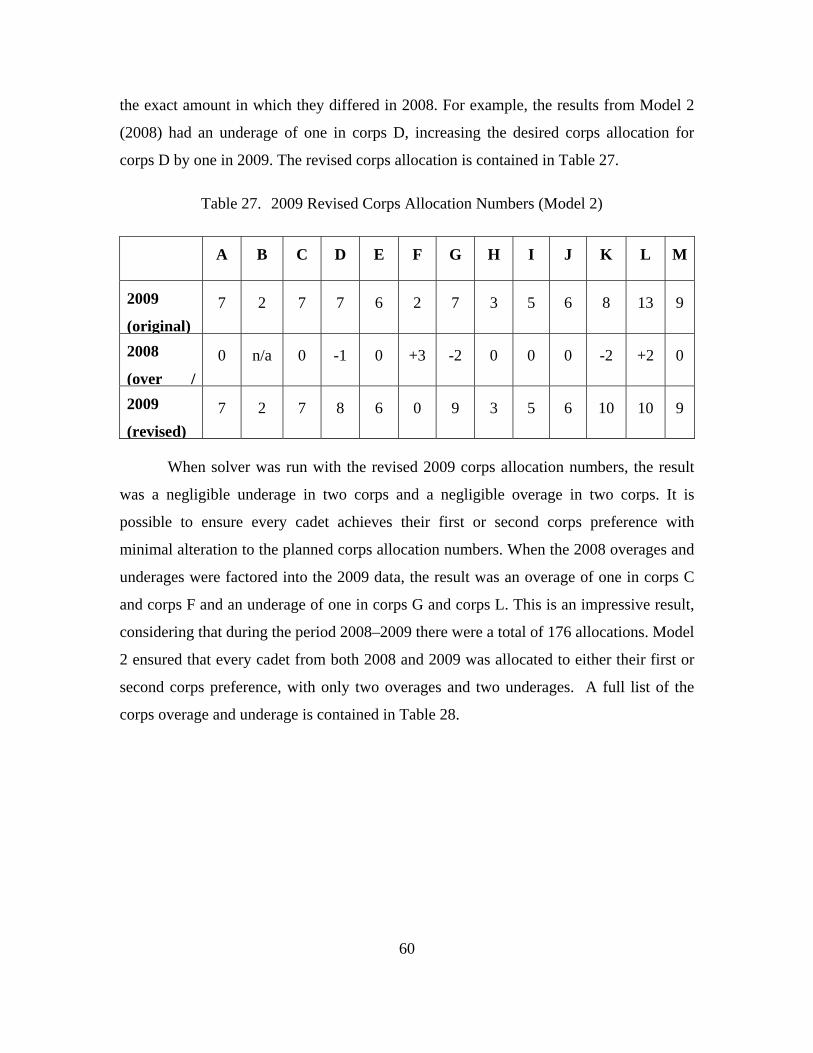
60

the exact amount in which they differed in 2008. For example, the results from Model 2

(2008) had an underage of one in corps D, increasing the desired corps allocation for

corps D by one in 2009. The revised corps allocation is contained in Table 27.

Table 27. 2009 Revised Corps Allocation Numbers (Model 2)


2009

(original)

7 2 7 7 6 2 7 3 5 6 8 13 9

2008

(over /

0 n/a 0 -1 0 +3 -2 0 0 0 -2 +2 0

2009

(revised)

7 2 7 8 6 0 9 3 5 6 10 10 9

When solver was run with the revised 2009 corps allocation numbers, the result

was a negligible underage in two corps and a negligible overage in two corps. It is

possible to ensure every cadet achieves their first or second corps preference with

minimal alteration to the planned corps allocation numbers. When the 2008 overages and

underages were factored into the 2009 data, the result was an overage of one in corps C

and corps F and an underage of one in corps G and corps L. This is an impressive result,

considering that during the period 2008–2009 there were a total of 176 allocations. Model

2 ensured that every cadet from both 2008 and 2009 was allocated to either their first or

second corps preference, with only two overages and two underages. A full list of the

corps overage and underage is contained in Table 28.

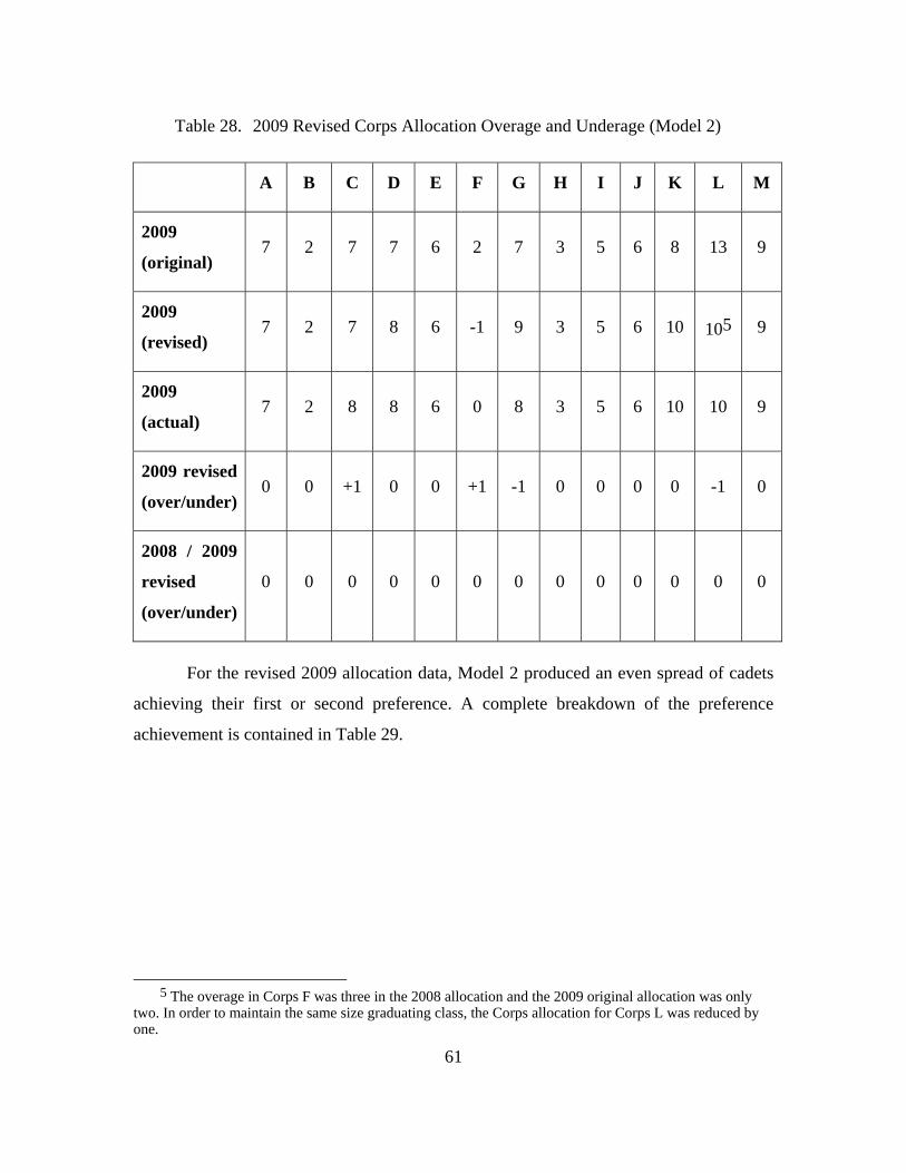
61

Table 28. 2009 Revised Corps Allocation Overage and Underage (Model 2)


2009

(original) 7 2 7 7 6 2 7 3 5 6 8 13 9

2009

(revised) 7 2 7 8 6 -1 9 3 5 6 10 105 9

2009

(actual) 7 2 8 8 6 0 8 3 5 6 10 10 9

2009 revised

(over/under) 0 0 +1 0 0 +1 -1 0 0 0 0 -1 0

2008 / 2009

revised

(over/under)

0 0 0 0 0 0 0 0 0 0 0 0 0

For the revised 2009 allocation data, Model 2 produced an even spread of cadets

achieving their first or second preference. A complete breakdown of the preference

achievement is contained in Table 29.

5 The overage in Corps F was three in the 2008 allocation and the 2009 original allocation was only

two. In order to maintain the same size graduating class, the Corps allocation for Corps L was reduced by one.

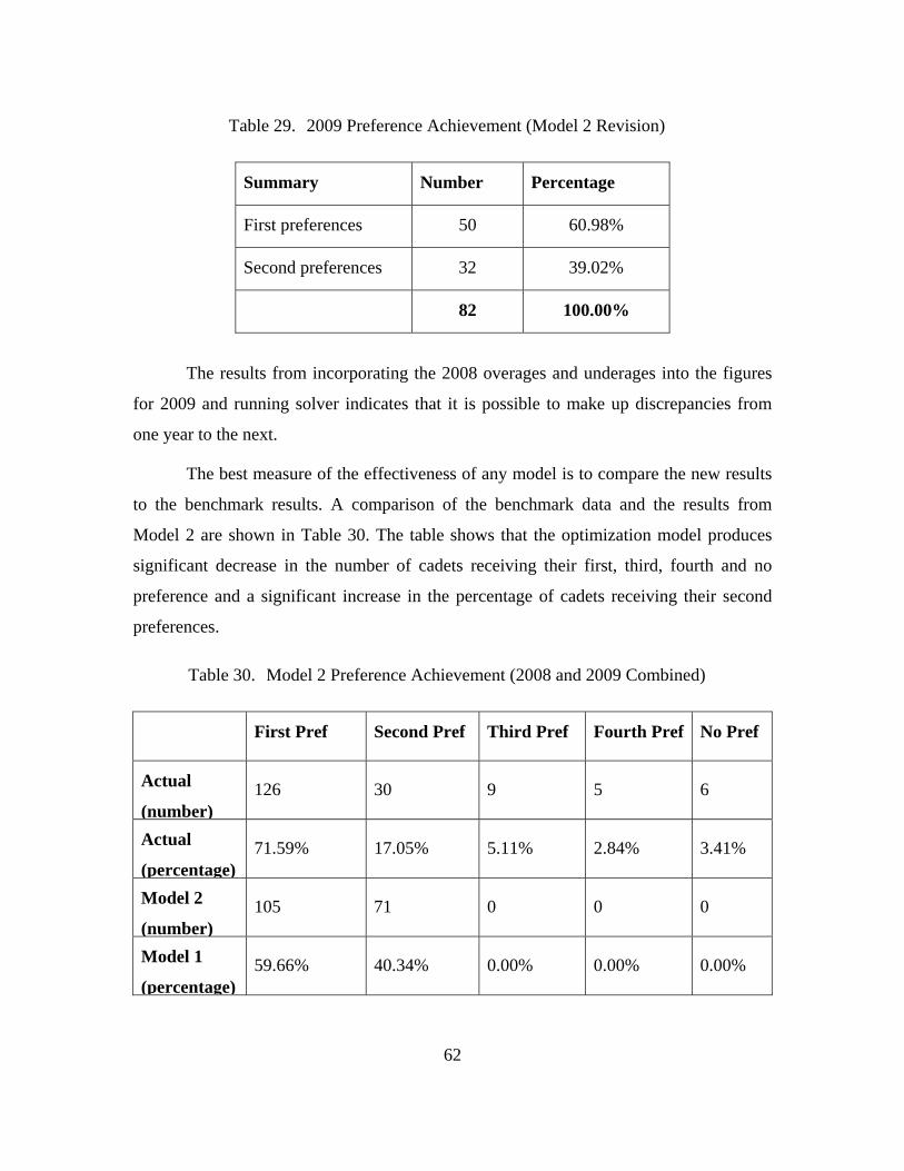
62

Table 29. 2009 Preference Achievement (Model 2 Revision)




82 100.00%

The results from incorporating the 2008 overages and underages into the figures

for 2009 and running solver indicates that it is possible to make up discrepancies from

one year to the next.


to the benchmark results. A comparison of the benchmark data and the results from

Model 2 are shown in Table 30. The table shows that the optimization model produces

significant decrease in the number of cadets receiving their first, third, fourth and no

preference and a significant increase in the percentage of cadets receiving their second

preferences.



Actual

(number) 126 30 9 5 6

Actual

(percentage) 71.59% 17.05% 5.11% 2.84% 3.41%

Model 2

(number) 105 71 0 0 0

Model 1

(percentage) 59.66% 40.34% 0.00% 0.00% 0.00%

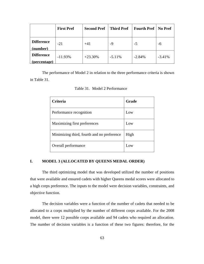
63


Difference

(number) -21 +41 -9 -5 -6

Difference

(percentage) -11.93% +23.30% -5.11% -2.84% -3.41%

The performance of Model 2 in relation to the three performance criteria is shown

in Table 31.


Criteria Grade

Performance recognition Low

Maximizing first preferences Low


Overall performance Low

I. MODEL 3 (ALLOCATED BY QUEENS MEDAL ORDER)

The third optimizing model that was developed utilized the number of positions

that were available and ensured cadets with higher Queens medal scores were allocated to

a high corps preference. The inputs to the model were decision variables, constraints, and

objective function.


allocated to a corps multiplied by the number of different corps available. For the 2008

model, there were 12 possible corps available and 94 cadets who required an allocation.

The number of decision variables is a function of these two figures: therefore, for the

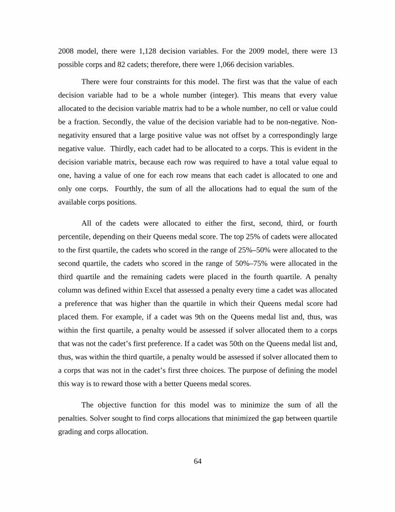
64

2008 model, there were 1,128 decision variables. For the 2009 model, there were 13

possible corps and 82 cadets; therefore, there were 1,066 decision variables.

There were four constraints for this model. The first was that the value of each

decision variable had to be a whole number (integer). This means that every value

allocated to the decision variable matrix had to be a whole number, no cell or value could

be a fraction. Secondly, the value of the decision variable had to be non-negative. Non-

negativity ensured that a large positive value was not offset by a correspondingly large

negative value. Thirdly, each cadet had to be allocated to a corps. This is evident in the

decision variable matrix, because each row was required to have a total value equal to

one, having a value of one for each row means that each cadet is allocated to one and

only one corps. Fourthly, the sum of all the allocations had to equal the sum of the

available corps positions.

All of the cadets were allocated to either the first, second, third, or fourth

percentile, depending on their Queens medal score. The top 25% of cadets were allocated

to the first quartile, the cadets who scored in the range of 25%–50% were allocated to the

second quartile, the cadets who scored in the range of 50%–75% were allocated in the

third quartile and the remaining cadets were placed in the fourth quartile. A penalty

column was defined within Excel that assessed a penalty every time a cadet was allocated

a preference that was higher than the quartile in which their Queens medal score had

placed them. For example, if a cadet was 9th on the Queens medal list and, thus, was

within the first quartile, a penalty would be assessed if solver allocated them to a corps

that was not the cadet’s first preference. If a cadet was 50th on the Queens medal list and,

thus, was within the third quartile, a penalty would be assessed if solver allocated them to

a corps that was not in the cadet’s first three choices. The purpose of defining the model

this way is to reward those with a better Queens medal scores.

The objective function for this model was to minimize the sum of all the

penalties. Solver sought to find corps allocations that minimized the gap between quartile

grading and corps allocation.

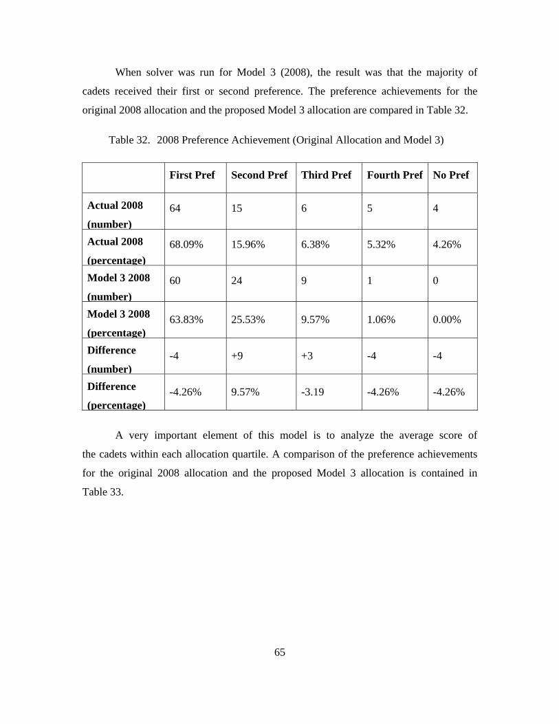
65

When solver was run for Model 3 (2008), the result was that the majority of

cadets received their first or second preference. The preference achievements for the

original 2008 allocation and the proposed Model 3 allocation are compared in Table 32.



Actual 2008

(number)

64 15 6 5 4

Actual 2008

(percentage)

68.09% 15.96% 6.38% 5.32% 4.26%

Model 3 2008

(number)

60 24 9 1 0

Model 3 2008

(percentage) 63.83% 25.53% 9.57% 1.06% 0.00%

Difference

(number) -4 +9 +3 -4 -4

Difference

(percentage) -4.26% 9.57% -3.19 -4.26% -4.26%

A very important element of this model is to analyze the average score of

the cadets within each allocation quartile. A comparison of the preference achievements

for the original 2008 allocation and the proposed Model 3 allocation is contained in

Table 33.

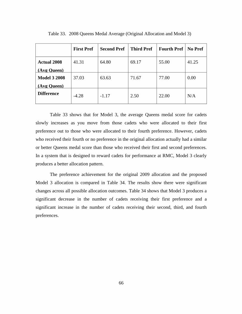
66

Table 33. 2008 Queens Medal Average (Original Allocation and Model 3)


Actual 2008

(Avg Queen)

41.31 64.80 69.17 55.00 41.25

Model 3 2008

(Avg Queen)

37.03 63.63 71.67 77.00 0.00

Difference -4.28 -1.17 2.50 22.00 N/A

Table 33 shows that for Model 3, the average Queens medal score for cadets

slowly increases as you move from those cadets who were allocated to their first

preference out to those who were allocated to their fourth preference. However, cadets

who received their fourth or no preference in the original allocation actually had a similar

or better Queens medal score than those who received their first and second preferences.

In a system that is designed to reward cadets for performance at RMC, Model 3 clearly

produces a better allocation pattern.

The preference achievement for the original 2009 allocation and the proposed

Model 3 allocation is compared in Table 34. The results show there were significant

changes across all possible allocation outcomes. Table 34 shows that Model 3 produces a

significant decrease in the number of cadets receiving their first preference and a

significant increase in the number of cadets receiving their second, third, and fourth

preferences.

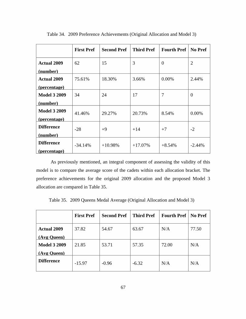
67

Table 34. 2009 Preference Achievements (Original Allocation and Model 3)


Actual 2009

(number)

62 15 3 0 2

Actual 2009

(percentage)

75.61% 18.30% 3.66% 0.00% 2.44%

Model 3 2009

(number)

34 24 17 7 0

Model 3 2009

(percentage) 41.46% 29.27% 20.73% 8.54% 0.00%

Difference

(number) -28 +9 +14 +7 -2

Difference

(percentage) -34.14% +10.98% +17.07% +8.54% -2.44%

As previously mentioned, an integral component of assessing the validity of this

model is to compare the average score of the cadets within each allocation bracket. The

preference achievements for the original 2009 allocation and the proposed Model 3

allocation are compared in Table 35.



Actual 2009

(Avg Queen)

37.82 54.67 63.67 N/A 77.50

Model 3 2009

(Avg Queen)

21.85 53.71 57.35 72.00 N/A

Difference -15.97 -0.96 -6.32 N/A N/A

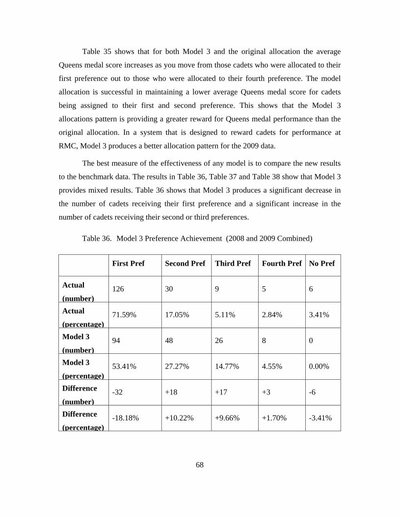
68

Table 35 shows that for both Model 3 and the original allocation the average

Queens medal score increases as you move from those cadets who were allocated to their

first preference out to those who were allocated to their fourth preference. The model

allocation is successful in maintaining a lower average Queens medal score for cadets

being assigned to their first and second preference. This shows that the Model 3

allocations pattern is providing a greater reward for Queens medal performance than the

original allocation. In a system that is designed to reward cadets for performance at

RMC, Model 3 produces a better allocation pattern for the 2009 data.


to the benchmark data. The results in Table 36, Table 37 and Table 38 show that Model 3

provides mixed results. Table 36 shows that Model 3 produces a significant decrease in

the number of cadets receiving their first preference and a significant increase in the

number of cadets receiving their second or third preferences.



Actual

(number) 126 30 9 5 6

Actual

(percentage) 71.59% 17.05% 5.11% 2.84% 3.41%

Model 3

(number) 94 48 26 8 0

Model 3

(percentage) 53.41% 27.27% 14.77% 4.55% 0.00%

Difference

(number) -32 +18 +17 +3 -6

Difference

(percentage) -18.18% +10.22% +9.66% +1.70% -3.41%

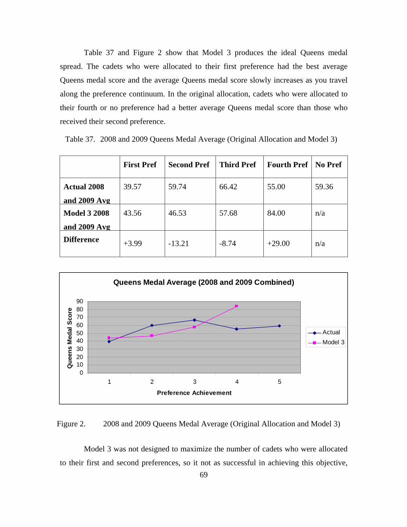
69

Table 37 and Figure 2 show that Model 3 produces the ideal Queens medal

spread. The cadets who were allocated to their first preference had the best average

Queens medal score and the average Queens medal score slowly increases as you travel

along the preference continuum. In the original allocation, cadets who were allocated to

their fourth or no preference had a better average Queens medal score than those who

received their second preference.

Table 37. 2008 and 2009 Queens Medal Average (Original Allocation and Model 3)


Actual 2008

and 2009 Avg

39.57 59.74 66.42 55.00 59.36

Model 3 2008

and 2009 Avg

43.56 46.53 57.68 84.00 n/a

Difference +3.99 -13.21 -8.74 +29.00 n/a

Queens Medal Average (2008 and 2009 Combined)

0102030405060708090

1 2 3 4 5

Preference Achievement

Qu

een

s M

edal

Sco

re

Actual

Model 3

Figure 2. 2008 and 2009 Queens Medal Average (Original Allocation and Model 3)

Model 3 was not designed to maximize the number of cadets who were allocated

to their first and second preferences, so it not as successful in achieving this objective,

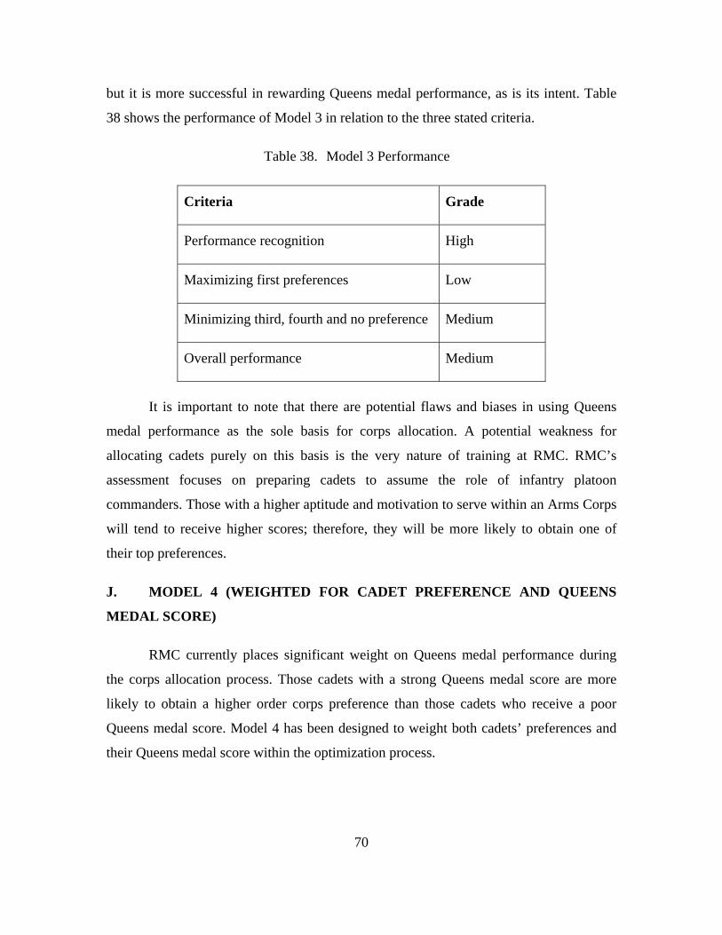
70

but it is more successful in rewarding Queens medal performance, as is its intent. Table

38 shows the performance of Model 3 in relation to the three stated criteria.


Criteria Grade

Performance recognition High

Maximizing first preferences Low

Minimizing third, fourth and no preference Medium

Overall performance Medium

It is important to note that there are potential flaws and biases in using Queens

medal performance as the sole basis for corps allocation. A potential weakness for

allocating cadets purely on this basis is the very nature of training at RMC. RMC’s

assessment focuses on preparing cadets to assume the role of infantry platoon

commanders. Those with a higher aptitude and motivation to serve within an Arms Corps

will tend to receive higher scores; therefore, they will be more likely to obtain one of

their top preferences.

J. MODEL 4 (WEIGHTED FOR CADET PREFERENCE AND QUEENS

MEDAL SCORE)

RMC currently places significant weight on Queens medal performance during

the corps allocation process. Those cadets with a strong Queens medal score are more

likely to obtain a higher order corps preference than those cadets who receive a poor

Queens medal score. Model 4 has been designed to weight both cadets’ preferences and

their Queens medal score within the optimization process.

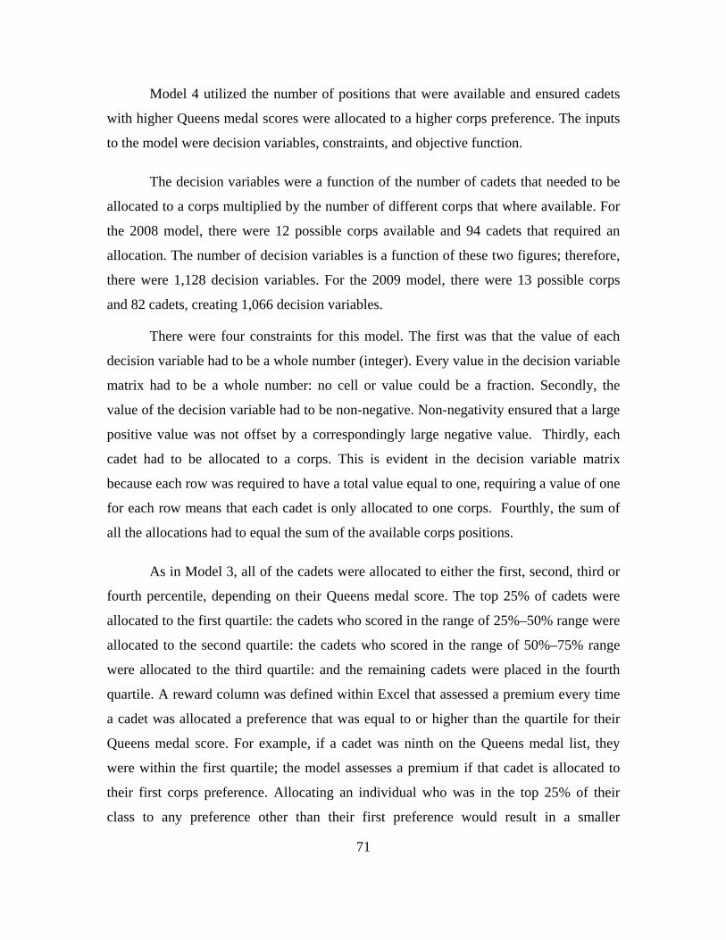
71

Model 4 utilized the number of positions that were available and ensured cadets

with higher Queens medal scores were allocated to a higher corps preference. The inputs

to the model were decision variables, constraints, and objective function.


allocated to a corps multiplied by the number of different corps that where available. For

the 2008 model, there were 12 possible corps available and 94 cadets that required an

allocation. The number of decision variables is a function of these two figures; therefore,

there were 1,128 decision variables. For the 2009 model, there were 13 possible corps

and 82 cadets, creating 1,066 decision variables.

There were four constraints for this model. The first was that the value of each

decision variable had to be a whole number (integer). Every value in the decision variable

matrix had to be a whole number: no cell or value could be a fraction. Secondly, the

value of the decision variable had to be non-negative. Non-negativity ensured that a large

positive value was not offset by a correspondingly large negative value. Thirdly, each

cadet had to be allocated to a corps. This is evident in the decision variable matrix

because each row was required to have a total value equal to one, requiring a value of one

for each row means that each cadet is only allocated to one corps. Fourthly, the sum of

all the allocations had to equal the sum of the available corps positions.

As in Model 3, all of the cadets were allocated to either the first, second, third or

fourth percentile, depending on their Queens medal score. The top 25% of cadets were

allocated to the first quartile: the cadets who scored in the range of 25%–50% range were

allocated to the second quartile: the cadets who scored in the range of 50%–75% range

were allocated to the third quartile: and the remaining cadets were placed in the fourth

quartile. A reward column was defined within Excel that assessed a premium every time

a cadet was allocated a preference that was equal to or higher than the quartile for their

Queens medal score. For example, if a cadet was ninth on the Queens medal list, they

were within the first quartile; the model assesses a premium if that cadet is allocated to

their first corps preference. Allocating an individual who was in the top 25% of their

class to any preference other than their first preference would result in a smaller

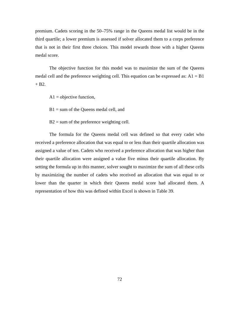
72

premium. Cadets scoring in the 50–75% range in the Queens medal list would be in the

third quartile; a lower premium is assessed if solver allocated them to a corps preference

that is not in their first three choices. This model rewards those with a higher Queens

medal score.

The objective function for this model was to maximize the sum of the Queens

medal cell and the preference weighting cell. This equation can be expressed as: A1 = B1

+ B2.

A1 = objective function,

B1 = sum of the Queens medal cell, and

B2 = sum of the preference weighting cell.

The formula for the Queens medal cell was defined so that every cadet who

received a preference allocation that was equal to or less than their quartile allocation was

assigned a value of ten. Cadets who received a preference allocation that was higher than

their quartile allocation were assigned a value five minus their quartile allocation. By

setting the formula up in this manner, solver sought to maximize the sum of all these cells

by maximizing the number of cadets who received an allocation that was equal to or

lower than the quarter in which their Queens medal score had allocated them. A

representation of how this was defined within Excel is shown in Table 39.

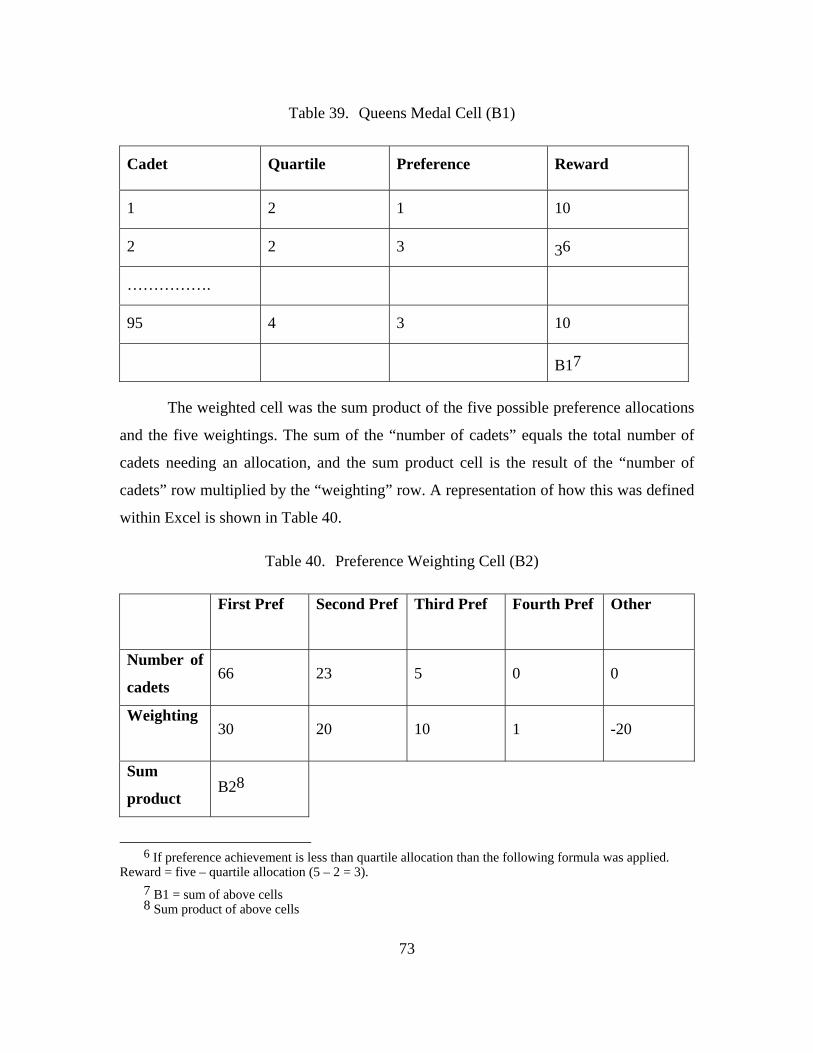
73

Table 39. Queens Medal Cell (B1)

Cadet Quartile Preference Reward

1 2 1 10

2 2 3 36

…………….

95 4 3 10

B17

The weighted cell was the sum product of the five possible preference allocations

and the five weightings. The sum of the “number of cadets” equals the total number of

cadets needing an allocation, and the sum product cell is the result of the “number of

cadets” row multiplied by the “weighting” row. A representation of how this was defined

within Excel is shown in Table 40.

Table 40. Preference Weighting Cell (B2)

First Pref Second Pref Third Pref Fourth Pref Other

Number of

cadets 66 23 5 0 0

Weighting

30 20 10 1 -20

Sum

product B28

6 If preference achievement is less than quartile allocation than the following formula was applied.

Reward = five – quartile allocation (5 – 2 = 3).

7 B1 = sum of above cells 8 Sum product of above cells

74

When solver was run for Model 4 (2008), the result was an increase in the number

of cadets receiving both their first and second preferences and there was a drop in the

number of cadets receiving their third, fourth, or no preference. For 2008, model 4

ensured 70% of cadets received their first choice corps, compared to 68% in the actual

allocation: only 5% of cadets would have received their third, fourth or no preference,

compared to 16% in the actual allocation. The actual 2008 preference achievement and

the Model 4 (2008) allocation are compared in Table 41.



Actual 2008

(number) 64 15 6 5 4

Actual 2008

(percentage) 68.09% 15.96% 6.38% 5.32% 4.26%

Model 4 2008

(number) 66 23 5 0 0

Model 4 2008

(percentage) 70.22% 24.49% 5.32% 0.00% 0.00%

Difference

(number) +2 +8 -1 -5 -4

Difference

(percentage) +2.13% +8.51% -1.06% -5.32% -4.26%

The purpose of Model 4 is to not only to maximize higher order preferences but it

also seeks to reward cadets with higher Queens medal ranking. Therefore, it is important

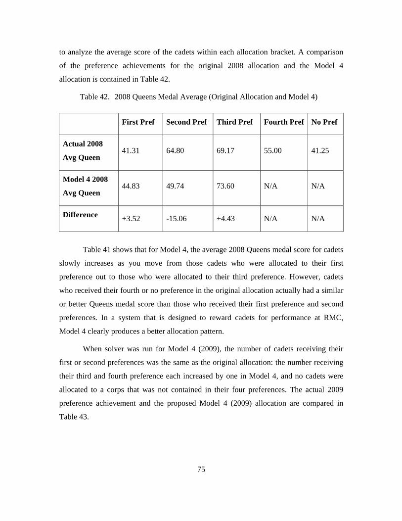
75

to analyze the average score of the cadets within each allocation bracket. A comparison

of the preference achievements for the original 2008 allocation and the Model 4

allocation is contained in Table 42.



Actual 2008

Avg Queen 41.31 64.80 69.17 55.00 41.25

Model 4 2008

Avg Queen 44.83 49.74 73.60 N/A N/A

Difference +3.52 -15.06 +4.43 N/A N/A

Table 41 shows that for Model 4, the average 2008 Queens medal score for cadets

slowly increases as you move from those cadets who were allocated to their first

preference out to those who were allocated to their third preference. However, cadets

who received their fourth or no preference in the original allocation actually had a similar

or better Queens medal score than those who received their first preference and second

preferences. In a system that is designed to reward cadets for performance at RMC,

Model 4 clearly produces a better allocation pattern.

When solver was run for Model 4 (2009), the number of cadets receiving their

first or second preferences was the same as the original allocation: the number receiving

their third and fourth preference each increased by one in Model 4, and no cadets were

allocated to a corps that was not contained in their four preferences. The actual 2009

preference achievement and the proposed Model 4 (2009) allocation are compared in

Table 43.

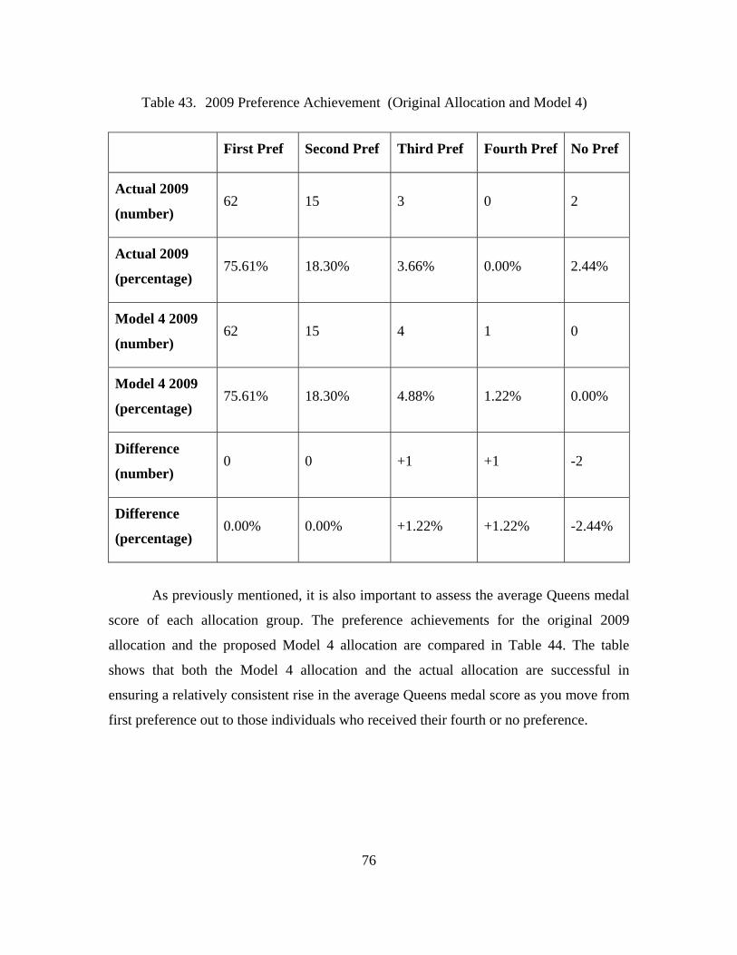
76



Actual 2009

(number) 62 15 3 0 2

Actual 2009

(percentage) 75.61% 18.30% 3.66% 0.00% 2.44%

Model 4 2009

(number) 62 15 4 1 0

Model 4 2009

(percentage) 75.61% 18.30% 4.88% 1.22% 0.00%

Difference

(number) 0 0 +1 +1 -2

Difference

(percentage) 0.00% 0.00% +1.22% +1.22% -2.44%

As previously mentioned, it is also important to assess the average Queens medal

score of each allocation group. The preference achievements for the original 2009

allocation and the proposed Model 4 allocation are compared in Table 44. The table

shows that both the Model 4 allocation and the actual allocation are successful in

ensuring a relatively consistent rise in the average Queens medal score as you move from

first preference out to those individuals who received their fourth or no preference.

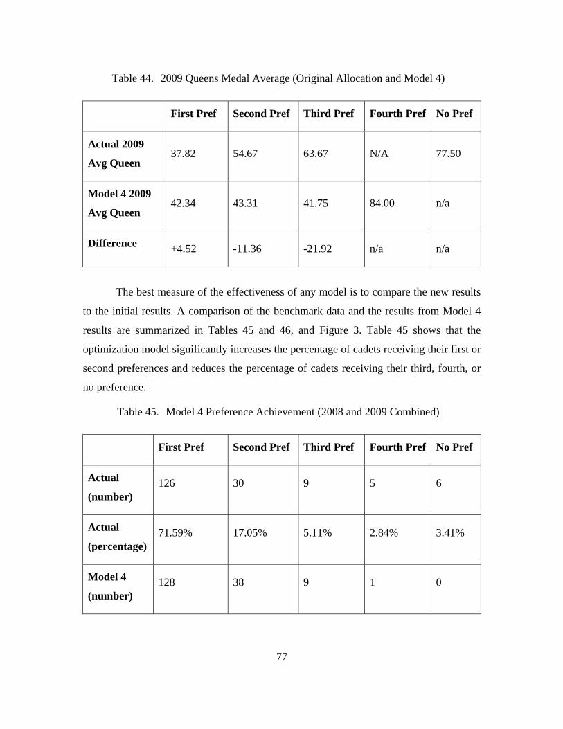
77



Actual 2009

Avg Queen 37.82 54.67 63.67 N/A 77.50

Model 4 2009

Avg Queen 42.34 43.31 41.75 84.00 n/a

Difference +4.52 -11.36 -21.92 n/a n/a


to the initial results. A comparison of the benchmark data and the results from Model 4

results are summarized in Tables 45 and 46, and Figure 3. Table 45 shows that the

optimization model significantly increases the percentage of cadets receiving their first or

second preferences and reduces the percentage of cadets receiving their third, fourth, or

no preference.



Actual

(number) 126 30 9 5 6

Actual

(percentage) 71.59% 17.05% 5.11% 2.84% 3.41%

Model 4

(number) 128 38 9 1 0

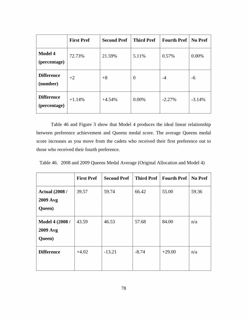
78


Model 4

(percentage) 72.73% 21.59% 5.11% 0.57% 0.00%

Difference

(number) +2 +8 0 -4 -6

Difference

(percentage) +1.14% +4.54% 0.00% -2.27% -3.14%

Table 46 and Figure 3 show that Model 4 produces the ideal linear relationship

between preference achievement and Queens medal score. The average Queens medal

score increases as you move from the cadets who received their first preference out to

those who received their fourth preference.

Table 46. 2008 and 2009 Queens Medal Average (Original Allocation and Model 4)


Actual (2008 /

2009 Avg

Queen)

39.57 59.74 66.42 55.00 59.36

Model 4 (2008 /

2009 Avg

Queen)

43.59 46.53 57.68 84.00 n/a

Difference +4.02 -13.21 -8.74 +29.00 n/a

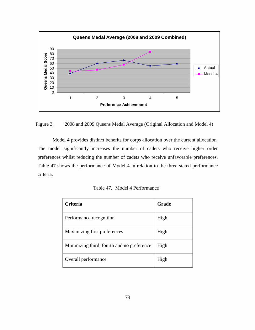
79

Figure 3. 2008 and 2009 Queens Medal Average (Original Allocation and Model 4)

Model 4 provides distinct benefits for corps allocation over the current allocation.

The model significantly increases the number of cadets who receive higher order

preferences whilst reducing the number of cadets who receive unfavorable preferences.

Table 47 shows the performance of Model 4 in relation to the three stated performance

criteria.


Criteria Grade

Performance recognition High

Maximizing first preferences High


Overall performance High

Queens Medal Average (2008 and 2009 Combined)

0102030405060708090

1 2 3 4 5

Preference Achievement

Qu

een

s M

edal

Sco

re

Actual

Model 4

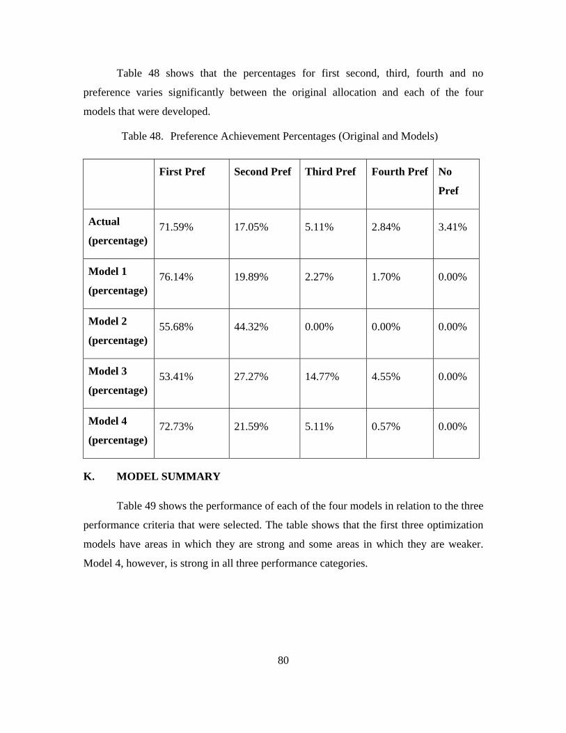
80

Table 48 shows that the percentages for first second, third, fourth and no

preference varies significantly between the original allocation and each of the four

models that were developed.

Table 48. Preference Achievement Percentages (Original and Models)

First Pref Second Pref Third Pref Fourth Pref No

Pref

Actual

(percentage) 71.59% 17.05% 5.11% 2.84% 3.41%

Model 1

(percentage) 76.14% 19.89% 2.27% 1.70% 0.00%

Model 2

(percentage) 55.68% 44.32% 0.00% 0.00% 0.00%

Model 3

(percentage) 53.41% 27.27% 14.77% 4.55% 0.00%

Model 4

(percentage) 72.73% 21.59% 5.11% 0.57% 0.00%

K. MODEL SUMMARY

Table 49 shows the performance of each of the four models in relation to the three

performance criteria that were selected. The table shows that the first three optimization

models have areas in which they are strong and some areas in which they are weaker.

Model 4, however, is strong in all three performance categories.

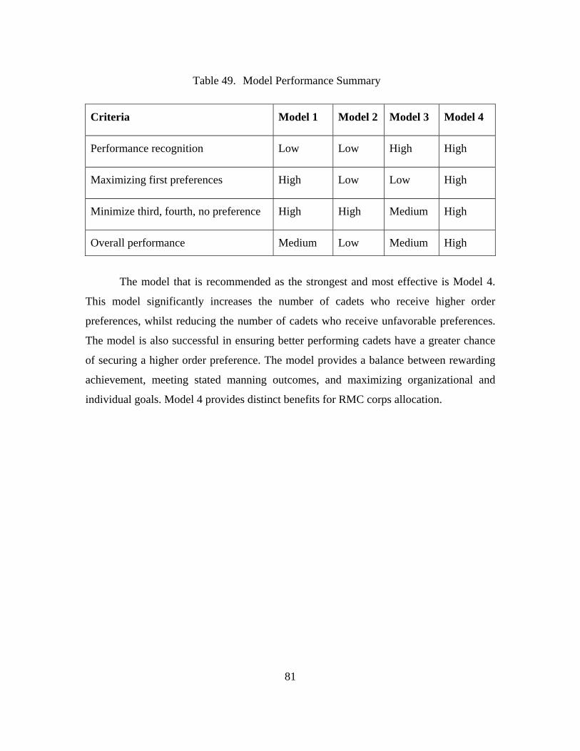
81

Table 49. Model Performance Summary

Criteria Model 1 Model 2 Model 3 Model 4

Performance recognition Low Low High High

Maximizing first preferences High Low Low High

Minimize third, fourth, no preference High High Medium High

Overall performance Medium Low Medium High

The model that is recommended as the strongest and most effective is Model 4.

This model significantly increases the number of cadets who receive higher order

preferences, whilst reducing the number of cadets who receive unfavorable preferences.

The model is also successful in ensuring better performing cadets have a greater chance

of securing a higher order preference. The model provides a balance between rewarding

achievement, meeting stated manning outcomes, and maximizing organizational and

individual goals. Model 4 provides distinct benefits for RMC corps allocation.

82


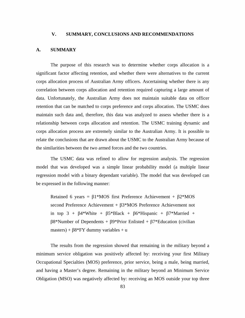
83

V. SUMMARY, CONCLUSIONS AND RECOMMENDATIONS

A. SUMMARY

The purpose of this research was to determine whether corps allocation is a

significant factor affecting retention, and whether there were alternatives to the current

corps allocation process of Australian Army officers. Ascertaining whether there is any

correlation between corps allocation and retention required capturing a large amount of

data. Unfortunately, the Australian Army does not maintain suitable data on officer

retention that can be matched to corps preference and corps allocation. The USMC does

maintain such data and, therefore, this data was analyzed to assess whether there is a

relationship between corps allocation and retention. The USMC training dynamic and

corps allocation process are extremely similar to the Australian Army. It is possible to

relate the conclusions that are drawn about the USMC to the Australian Army because of

the similarities between the two armed forces and the two countries.

The USMC data was refined to allow for regression analysis. The regression

model that was developed was a simple linear probability model (a multiple linear

regression model with a binary dependant variable). The model that was developed can

be expressed in the following manner:

Retained 6 years = β1*MOS first Preference Achievement + β2*MOS

second Preference Achievement + β3*MOS Preference Achievement not

in top 3 + β4*White + β5*Black + β6*Hispanic + β7*Married +

β8*Number of Dependents + β9*Prior Enlisted + β7*Education (civilian

masters) + β8*FY dummy variables + u

The results from the regression showed that remaining in the military beyond a

minimum service obligation was positively affected by: receiving your first Military

Occupational Specialties (MOS) preference, prior service, being a male, being married,

and having a Master’s degree. Remaining in the military beyond an Minimum Service

Obligation (MSO) was negatively affected by: receiving an MOS outside your top three

84

preferences, being Hispanic, and having a higher number of dependents. The results from

the six-year regression model verified that allocating cadets to an MOS of their choice is

a very important element within the retention framework of military officers.

The cost of training each Royal Military College (RMC) cadet to become an

officer in the Australian Army is extremely high. It is imperative to make every effort to

provide each cadet with a rewarding career in their chosen field. The first step in this

process is achieving a corps allocation that maximizes the cadets’ preferences whilst also

meeting the Army’s requirements. The optimization models that were developed in

Chapter IV will help reduce the workload on RMC staff and also ensure the best possible

outcome for both RMC cadets and the Australian Army.

Optimization models were developed that maximized cadet preferences whilst

also meeting service requirements. Data from cadets who graduated from RMC in 2008

and 2009 was utilized to develop more robust and effective allocation models. The

models showed significant increases in those cadets who received their first or second

preference and significant decreases in cadets being allocated to the third, fourth, or other

preferences.

The first optimizing model that was developed sought to emphasize allocating

each cadet to one of their highest preferences by maximizing the weighted average score

of allocations. The weightings assigned were 25, 15, 5, 1, and -20 for an allocation to the

first, second, third, fourth and other preference, respectively. Compared to the original

data, Model 1 significantly increased the number of cadets who received higher order

preferences whilst reducing the number of cadets who received unfavorable preferences.

The problem with Model 1 is that it does not consider a cadet’s performance or Queens

medal score in the allocation. Recognition and reward of performance is seen as a key

element of Australian Army officer training. It is important to note that many countries

throughout the world have intentionally removed training performance from the corps

allocation process. The benefit of excluding performance as a driver for the allocation

process is that it aids in the even distribution of talent throughout each of the separate

85

corps. The militaries of countries such as the United States have developed policies that

ensure each of their corps is allocated an appropriate mix of both higher performing and

lower performing officers.

The second optimization model ensured each cadet received an allocation that

was either their first or second corps preferences. This model was developed to address

the regression results that were obtained in Chapter III: a linear probability model that

utilized USMC data. The results showed that remaining in the military beyond a

minimum service obligation was positively affected by receiving your first MOS

preference.

Model 2 showed that it was possible to ensure every cadet achieves their first or

second corps preference with minimal alteration to the planned corps allocation numbers.

Furthermore, the model showed that a corps overage or underage from one year could be

resolved in the following year. When Model 2 was run for the actual RMC data from

2008 and 2009, the result after the 2009 allocation was an overage of one in corps C and

corps F and an underage of one in corps G and corps L. This is an impressive result

considering that over the period 2008–2009 there were a total of 176 allocations. Model 2

allocated every cadet from both 2008 and 2009 to either their first or second corps

preference, with only two overages and two underages.

The third optimization model ensured cadets with higher Queens medal scores

were allocated to a high corps preference. The results in Tables 33 and 34 show that

Model 3 provided mixed results. The tables show that Model 3 produced a significant

decrease in the number of cadets receiving their first preference and a significant increase

in the number of cadets receiving their second or third preferences. Table 34 shows that

Model 3 produces a more effective Queens medal spread. The cadets who were allocated

to their first preference had the best average Queens medal score; the average Queens

medal score slowly increases as you travel along the preference continuum. Model 3 is

not as successful in its spread of preference achievement but it is successful in rewarding

performance (Queens medal score).

86

Model 4 was the final model that was developed, and it weighted both the cadet’s

preferences and their Queens medal score within the optimization process. This model

significantly increases the number of cadets who receive higher order preferences whilst

reducing the number of cadets who receive unfavorable preferences. Model 4 produced a

strong linear relationship between preference achievement and Queens medal score. The

average Queens medal score slowly increases as you move from the cadets who received

their first preference out to those who received their fourth preference. Model 4 provides

distinct benefits for the RMC corps allocation. The model provides a balance between

rewarding achievement, meeting stated manning outcomes, and maximizing

organizational and individual goals.

Table 50 provides a summary of the preference achievements for the actual

allocation and for each of the four models that were developed.

Table 50. Preference Achievement Percentages (Original and Models)


Actual

(percentage) 71.59% 17.05% 5.11% 2.84% 3.41%

Model 1

(percentage) 76.14% 19.89% 2.27% 1.70% 0.00%

Model 2

(percentage) 55.68% 44.32% 0.00% 0.00% 0.00%

Model 3

(percentage) 53.41% 27.27% 14.77% 4.55% 0.00%

Model 4

(percentage) 72.73% 21.59% 5.11% 0.57% 0.00%

87

B. CONCLUSIONS AND RECOMMENDATIONS

This research has proven there is a definite link between corps allocation and

retention dynamics. The Australian Army should incorporate optimization modeling into

the corps allocation process; the model that is recommended is Model 4. The basis of

Model 4 was that it sought to maximize higher order cadet preferences whilst adhering to

the number of positions available within each corps. When Model 4 was run with the

actual data from 2008 and 2009, it offered a significant increase in the percentage of

cadets receiving their first or second preferences and a significant reduction in the

percentage of cadets receiving their third, fourth, or no preference. It also was sensitive to

the Queens medal ranking, emphasizing preferences for those with better Queens medal

scores. By significantly increasing the number of cadets who receive higher order

preferences whilst reducing the number of cadets who receive unfavorable preferences,

the model improves the potential for retention beyond an officer’s minimum return of

service obligation.

1. Primary Research Question

The primary research question that this thesis sought to answer was, does a

cadet’s allocation to either their first, second, third, or fourth corps preference affect their

propensity to discharge? The literature research and regression analysis prove that there is

a strong link between preference achievement and retention dynamics. Cadets who

receive their first preference are far more likely to remain after their MSO than those

cadets who receive their third, fourth or none of their preferences.

2. Secondary Research Questions

The secondary research question was whether there are alternatives to the current

corps allocation process in the Australian Army? The four models that were developed in

Chapter IV show that there are alternatives to the current corps allocation process. The

model were able to place emphasis on either Queens medal score, maximizing higher

order preferences, minimizing lower order preferences or completely eliminating lower

order preferences. The models provide an efficient and effective tool that staff at the

88

Royal military College (RMC) can use to help guide the corps allocation of cadets. The

models are not intended to replace staff input into the corps allocation process; rather

they are intended to relieve some of the workload.

C. RECOMMENDATION FOR FURTHER STUDY

Further experiments could strengthen and confirm the model results that were

achieved in Chapter IV. The Australian Army should look to use the Monte Carlo method

to assess the effectiveness of the optimization Model 4. A Monte Carlo method is a

technique that involves using random numbers to solve problems. Monte Carlo methods

are often used in simulating mathematical problems. Monte Carlo methods are very

useful because of their reliance on repeated computations of random or pseudo-random

numbers. Using Monte Carlo would enable random cadet corps preferences to be

generated. These preferences could then be inputted into Model 4 to access the preference

achievement of the model. Not relying solely on actual data and instead using the new

Monte Carlo generated data would enable unlimited testing of Model 4.

89

LIST OF REFERENCES

Arnold, H.J., & Feldman, D.C. (1982). A multivariate analysis of the job turnover process. Journal of Applied Psychology, Vol 67, 350–360.

Abrahams, N.M., Githens, W.H., & Neumann, I. (1998). The Measurement of Naval Career Motivation in NROTC Applicants. San Diego: U.S. Naval Personnel Research Activity.

Blackmon, J.L. (2009). The effect of MOS selection and placement on the retention of marine company officers. Master’s thesis, Naval Postgraduate School, Monterey, CA.

Cotton, J.L. & Tuttle, J.M. (1986). Employee turnover: A meta-analysis and review with implications research. The Academy of Management Review, Vol 11(1), 55–70.

Carbone, E.G., Cigrang, J.A., Todd, S.L., & Fiedler, E.R. (1999). Predicting outcome of military basic training for individuals referred for psychological evaluation, Journal of Personality Assessment, Vol 72.

Jaquette, D.L., & Nelson, G.R. (1974). The implications of manpower supply and productivity for the pay and composition of the military force: An optimization model. RAND Corporation, R-1451-ARPA.

Gotz, G.A. & McCall, J.J. (1984). A dynamic retention model for air force officers: Theory and estimates, RAND Corporation, R-3028-AF.

Lakhani. H (1991). Retention cost-benefit analysis of U.S army junior officers a multidisciplinary analysis,” Journal of Political and Military Sociology, Vol 19.

March, J.C., & Simon, H.A. (1958). Organizations. Wiley, New York.

Marsh, R.M. (1989). Predicting retention in the U.S navy: officers and enlisted. Journal of Political and Military Sociology, Vol 17.

Mobley W. H. (1977). Intermediate linkages in the relationship between job satisfaction and employee turnover.” Journal of Applied Psychology, Vol 62.

Mobley, W. H., Griffeth, R. W., Hand, H. H., & Meglino, B. M. (1979). Review and conceptual analysis of the employee turnover process. Psychological Bulletin, Vol 86, 493–522.

Mowbay, R.T., Porter, L.W., & Steers, R.M. (1982). Employee and organizational linkages, New York, NY: Academic Press.

Porter, L.W., & Steers, R.M. (1973). Organizational, work, and personal factors in employee turnover and absenteeism. Psychological Bulletin, Vol 80.

90

Pearson, C.A.L. (1995). The turnover process in organizations: an exploration of the role of unmet expectations. Human Relations. Vol 48(4),

Rousseau, D., & Geller, M. (1994). Human resource practices: administrative contract makers", Human Resource Management, Vol 33, 385–402.

Sims, R.R (1994). Human resource management’s role in clarifying the new psychological contract. Human Resource Management, 33(3), 373–382.

91

INITIAL DISTRIBUTION LIST

1. Dudley Knox Library

Naval Postgraduate School Monterey, California

2. Captain (RAN) Brett Wolski Directorate of Workforce Modeling & Analysis Canberra, Australian Capital Territory Australia

3. Lieutenant Colonel Phillip Hoglin Directorate of Workforce Modeling & Analysis - Army Canberra, Australian Capital Territory Australia

4. Library Australian Defence Force Academy Canberra, Australian Capital Territory Australia

5. Dean William Gates Naval Postgraduate School Monterey, California

6. Professor William Hatch Naval Postgraduate School Monterey, California

7. Major David Nelson

Directorate of Workforce Modeling & Analysis - Army Canberra, Australian Capital Territory Australia

8. Brigadier Mick Moon, DSC, AM

Royal Military College Canberra, Australian Capital Territory Australia

Documents

NAVAL POSTGRADUATE SCHOOL - apps.dtic.mil · i REPORT DOCUMENTATION PAGE Form Approved OMB No. 0704-0188 Public reporting burden for this collection of information is estimated to