Embed Size (px)
Citation preview
NAVAL POSTGRADUATE
SCHOOL
MONTEREY, CALIFORNIA
THESIS
Approved for public release; distribution is unlimited
PERFORMANCE ANALYSIS OF THE EFFECT OF PULSED-NOISE INTERFERENCE ON WLAN SIGNALS
TRANSMITTED OVER A NAKAGAMI FADING CHANNEL
by Andreas Tsoumanis
March 2004
Thesis Advisor: R. Clark Robertson Second Reader: Donald Wadsworth

THIS PAGE INTENTIONALLY LEFT BLANK

i
REPORT DOCUMENTATION PAGE Form Approved OMB No. 0704-0188 Public reporting burden for this collection of information is estimated to average 1 hour per response, including the time for reviewing instruction, searching existing data sources, gathering and maintaining the data needed, and completing and reviewing the collection of information. Send comments regarding this burden estimate or any other aspect of this collection of information, including suggestions for reducing this burden, to Washington headquarters Services, Directorate for Information Operations and Reports, 1215 Jefferson Davis Highway, Suite 1204, Arlington, VA 22202-4302, and to the Office of Management and Budget, Paperwork Reduction Project (0704-0188) Washington DC 20503. 1. AGENCY USE ONLY (Leave blank)
2. REPORT DATE March 2004
3. REPORT TYPE AND DATES COVERED Master’s Thesis
4. TITLE AND SUBTITLE: Title (Mix case letters) Performance Analysis of the Effect of Pulsed-noise Interference on WLAN Signals Transmitted over a Nakagami Fading Channel.
6. AUTHOR Andreas Tsoumanis
5. FUNDING NUMBERS
7. PERFORMING ORGANIZATION NAME AND ADDRESS Naval Postgraduate School Monterey, CA 93943-5000
8. PERFORMING ORGANIZATION REPORT NUMBER
9. SPONSORING /MONITORING AGENCY NAME AND ADDRESS35 N/A
10. SPONSORING/MONITORING AGENCY REPORT NUMBER
11. SUPPLEMENTARY NOTES The views expressed in this thesis are those of the author and do not reflect the official policy or position of the Department of Defense or the U.S. Government. 12a. DISTRIBUTION / AVAILABILITY STATEMENT
Approved for public release; distribution is unlimited. 12b. DISTRIBUTION CODE
13. ABSTRACT (maximum 200 words) This thesis examines the performance of wireless local area network (WLAN) signals, specifically, the signal of IEEE 802.11a standard. The signal is subject to pulsed-noise jamming, when either the desired signal alone or the desired signal and the jamming signal are subject to Nakagami fading. As expected, the implementation of forward error correction (FEC) coding with soft decision decoding (SDD) and maximum-likelihood detection improves performance as compared to uncoded signals. In addition, the combination of maximum-likelihood detection and error correction coding renders pulsed-noise jamming inef-fective as compared to barrage noise jamming. When the jamming signal encounters fading as well, we assume that the aver-age jamming power is much greater than the AWGN power. For uncoded signals, a jamming signal that experiences fading actually improves performance when the parameter of the information signal ms is less than or equal to one. Surprisingly, for larger values of ms a jamming signal that experiences fading works in favor of the information signal only for small signal-to-interference ratio (SIR). When SIR is large, performance when the jamming signal experiences fading is worse relative to per-formance when the jamming signal does not experience fading. For error correction coding with SDD, we investigate only continuous jamming since it is by far the worst-case. Moreover, while we consider a range of fading conditions for the jam-ming signal, we examine only Rayleigh fading of the information signal. The coded signal, when the jamming signal experi-ences severe fading, performs better relative to the case when the jamming signal does not experience fading.
15. NUMBER OF PAGES
87
14. SUBJECT TERMS IEEE 802.11a, WLAN, FEC, SDD, OFDM, BPSK, QPSK, MQAM, AWGN, Nakagami, soft decision decoding, convolutional code, pulsed-noise jamming, probability of bit error
16. PRICE CODE
17. SECURITY CLASSIFICATION OF REPORT
Unclassified
18. SECURITY CLASSIFICATION OF THIS PAGE
Unclassified
19. SECURITY CLASSIFICATION OF ABSTRACT
Unclassified
20. LIMITATION OF ABSTRACT
UL
NSN 7540-01-280-5500 Standard Form 298 (Rev. 2-89) Prescribed by ANSI Std. 239-18

ii
THIS PAGE INTENTIONALLY LEFT BLANK
iii
Approved for public release; distribution is unlimited
PERFORMANCE ANALYSIS OF THE EFFECT OF PULSE-NOISE INTERFERENCE ON WLAN SIGNALS TRANSMITTED OVER A NAKAGAMI
FADING CHANNEL
Andreas Tsoumanis Lieutenant Junior Grade, Hellenic Navy
B.S., Hellenic Naval Academy, 1996
Submitted in partial fulfillment of the requirements for the degree of
MASTER OF SCIENCE IN ELECTRICAL ENGINEERING and
MASTER OF SCIENCE IN SYSTEMS ENGINEERING
from the
NAVAL POSTGRADUATE SCHOOL March 2004
Author: Andreas Tsoumanis
Approved by: R. Clark Robertson
Thesis Advisor
Donald Wadsworth Co-Advisor
Dan C. Boger Chairman, Department of Information Sciences John P. Powers Chairman, Department of Electrical and Computer Engineering

iv
THIS PAGE INTENTIONALLY LEFT BLANK
v
ABSTRACT
This thesis examines the performance of wireless local area network (WLAN)
signals, specifically, the signal of IEEE 802.11a standard. The signal is subject to pulsed-
noise jamming, when either the desired signal alone or the desired signal and the jam-
ming signal are subject to Nakagami fading. As expected, the implementation of forward
error correction (FEC) coding with soft decision decoding (SDD) and maximum-
likelihood detection improves performance as compared to uncoded signals. In addition,
the combination of maximum-likelihood detection and error correction coding renders
pulsed-noise jamming ineffective as compared to barrage noise jamming. When the jam-
ming signal encounters fading as well, we assume that the average jamming power is
much greater than the AWGN power. For uncoded signals, a jamming signal that experi-
ences fading actually improves performance when the parameter of the information sig-
nal sm is less than or equal to one. Surprisingly, for larger values of sm a jamming signal
that experiences fading works in favor of the information signal only for small signal-to-
interference ratio (SIR). When SIR is large, performance when the jamming signal ex-
periences fading is worse relative to performance when the jamming signal does not ex-
perience fading. For error correction coding with SDD, we investigate only continuous
jamming since it is by far the worst-case. Moreover, while we consider a range of fading
conditions for the jamming signal, we examine only Rayleigh fading of the information
signal. The coded signal, when the jamming signal experiences severe fading, performs
better relative to the case when the jamming signal does not experience fading.

vi
THIS PAGE INTENTIONALLY LEFT BLANK
vii
TABLE OF CONTENTS
I. INTRODUCTION........................................................................................................1 A. OBJECTIVE ....................................................................................................1 B. RELATED RESEARCH.................................................................................2 C. THESIS ORGANIZATION............................................................................2
II. THEORY REVIEW.....................................................................................................5 A. INTRODUCTION............................................................................................5 B. NAKAGAMI FADING MODEL....................................................................5 C. WAVEFORM CHARACTERISTICS...........................................................6
1. Single Carrier Modulation Types.......................................................6 2. Forward Error Correction (FEC) ......................................................8 3. Orthogonal Frequency-Division Multiplexing (OFDM) ..................9
D. SUMMARY ....................................................................................................11
III. PERFORMANCE ANALYSIS WITH FEC AND SDD FOR SIGNALS TRANSMITTED OVER A NAKAGAMI FADING CHANNEL WITH PULSED-NOISE JAMMING...................................................................................13 A. INTRODUCTION..........................................................................................13 B. BPSK/QPSK ...................................................................................................13
1. Without SDD ......................................................................................13 2. With FEC and SDD ...........................................................................16
C. 16QAM/64QAM.............................................................................................31 1. Without FEC and SDD......................................................................31 2. With FEC and SDD ...........................................................................33
D. OFDM SYSTEM PERFORMANCE ...........................................................36 1. BPSK/QPSK .......................................................................................37 2. 16QAM/64QAM.................................................................................38
E. SUMMARY ....................................................................................................40
IV. PERFORMANCE ANALYSIS WITH FEC AND SDD, NAKAGAMI FADING CHANNELS, AND FADED PULSED-NOISE JAMMING..................41 A. INTRODUCTION..........................................................................................41 B. BPSK/QPSK ...................................................................................................41
1. Without FEC ......................................................................................41 2. With FEC and SDD ...........................................................................47 3. Comparison of BPSK/QPSK with and without FEC and SDD .....56
C. 16QAM/64QAM.............................................................................................57 D. SUMMARY OF FADED JAMMING..........................................................60
V. CONCLUSION ..........................................................................................................63 A. INTRODUCTION..........................................................................................63 B. FINDINGS......................................................................................................63 C. RECOMMENDATIONS FOR FURTHER RESEARCH .........................64

viii
D. CLOSING COMMENTS ..............................................................................64
LIST OF REFERENCES......................................................................................................67
INITIAL DISTRIBUTION LIST .........................................................................................69
ix
LIST OF FIGURES
Figure 1. The Nakagami probability density function [After Ref. 8.]...............................6 Figure 2. Constellation for BPSK, QPSK, 16QAM, and 64QAM [From Ref. 10.]..........7 Figure 3. Convolutional encoder with 7ν = and 1/ 2r = , where the empty boxes
denote shift registers [After Ref. 10.]. ...............................................................9 Figure 4. Transmitter and receiver block diagram for the OFDM PHY [After Ref.
10.]. ..................................................................................................................11 Figure 5. BPSK/QPSK for SNR 10= dB and 0.5p = [After Ref. 4.]. ...........................14 Figure 6. BPSK/QPSK for SNR 10= dB, and 1m = [After Ref. 4.]. .............................15 Figure 7. BPSK/QPSK for SNR 10= dB, 5m = , and 0.5p = [After Ref. 4.]. ..............16 Figure 8. BPSK/QPSK ( 1/ 2r = ) with FEC and SDD for signals transmitted over a
Nakagami fading channel ( 1m = ) with pulsed-noise jamming (SNR 10= dB)..................................................................................................26
Figure 9. BPSK/QPSK ( 1/ 2r = ) with FEC and SDD for signals transmitted over a Nakagami fading channel ( 1m = ) with pulsed-noise jamming (SNR 16= dB)..................................................................................................26
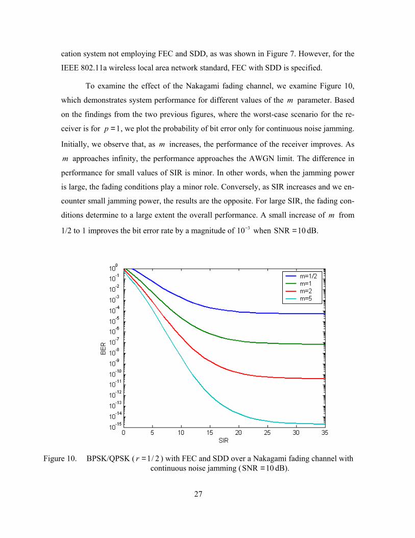
Figure 10. BPSK/QPSK ( 1/ 2r = ) with FEC and SDD over a Nakagami fading channel with continuous noise jamming (SNR 10= dB).................................27
Figure 11. BPSK/QPSK ( 3 / 4r = ) with FEC and SDD over a Nakagami fading channel ( 1m = ) with pulsed-noise jamming (SNR 10= dB)...........................28
Figure 12. BPSK/QPSK ( 3 / 4r = ) with FEC and SDD over a Nakagami fading channel ( 1m = ) with pulsed-noise jamming (SNR 16= dB)...........................29
Figure 13. BPSK/QPSK ( 3 / 4r = ) vs. 1/ 2r = with FEC and SDD over a Nakagami fading channel with continuous noise jamming (SNR 10= dB)......................29
Figure 14. BPSK/QPSK ( 1/ 2r = ) with FEC and SDD over a Nakagami fading channel with continuous noise jamming (SNR 10= dB) vs. uncoded performance. ....................................................................................................30
Figure 15. BPSK/QPSK ( 3 / 4r = ) with FEC and SDD over a Nakagami fading channel with continuous noise jamming (SNR 10= dB) vs. uncoded performance. ....................................................................................................31
Figure 16. 16QAM transmitted over a Nakagami fading channel with pulsed-noise jamming, SNR 10= dB, and 0.5p = [After Ref. 4.].......................................32
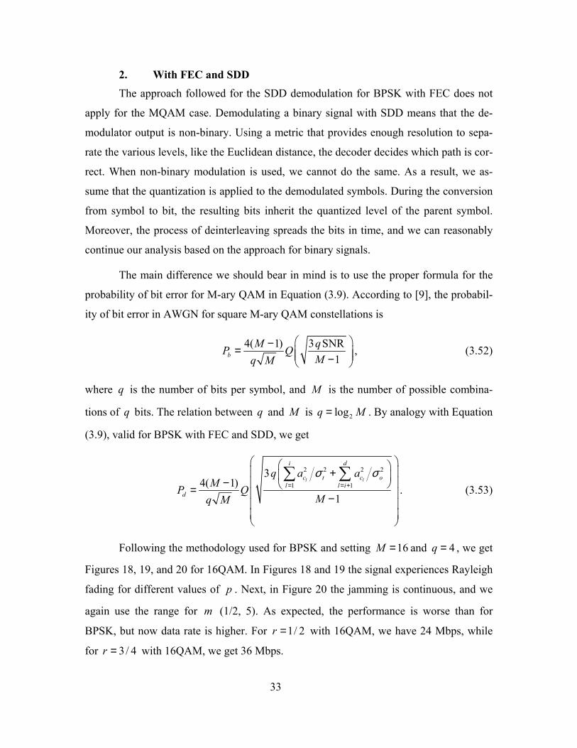
Figure 17. 64QAM transmitted over a Nakagami fading channel with pulsed-noise jamming, SNR 20= dB, and 0.5p = [After Ref. 4.]. .....................................32
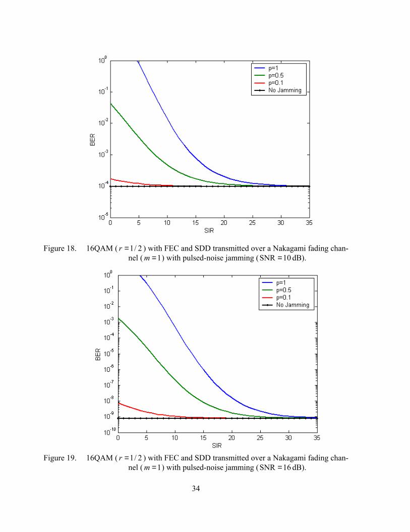
Figure 18. 16QAM ( 1/ 2r = ) with FEC and SDD transmitted over a Nakagami fading channel ( 1m = ) with pulsed-noise jamming (SNR 10= dB). ..............34
Figure 19. 16QAM ( 1/ 2r = ) with FEC and SDD transmitted over a Nakagami fading channel ( 1m = ) with pulsed-noise jamming (SNR 16= dB). ..............34
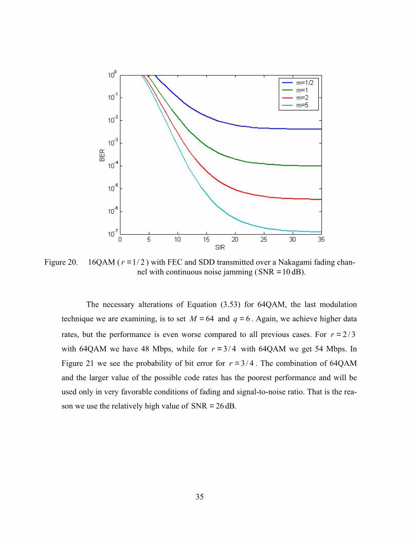
Figure 20. 16QAM ( 1/ 2r = ) with FEC and SDD transmitted over a Nakagami fading channel with continuous noise jamming (SNR 10= dB)......................35
x
Figure 21. 64QAM ( 3/ 4r = ) with FEC and SDD transmitted over a Nakagami fading channel with 1m = (Rayleigh fading), and SNR 26= dB....................36
Figure 22. OFDM BPSK ( 1/ 2r = ) with FEC and SDD (SNR 10= dB). ........................37 Figure 23. OFDM BPSK ( 1/ 2r = ) with FEC and SDD (SNR 16= dB). ........................38 Figure 24. OFDM 16QAM ( 1/ 2r = ) with FEC and SDD (SNR 10= dB). .....................39 Figure 25. OFDM 16QAM ( 3/ 4r = ) with FEC and SDD (SNR 16= dB). ....................39 Figure 26. Performance of BPSK/QPSK ( 1/ 2sm = ) when the jamming signal
experiences Nakagami fading. .........................................................................44 Figure 27. Performance of BPSK/QPSK ( 1sm = ) when the jamming signal
experiences Nakagami fading. .........................................................................45 Figure 28. Performance of BPSK/QPSK ( 2sm = ) when the jamming signal
experiences Nakagami fading. .........................................................................46 Figure 29. Performance of BPSK/QPSK ( 3sm = ) when the jamming signal
experiences Nakagami fading. .........................................................................46 Figure 30. Performance of BPSK/QPSK with FEC and SDD for 1sm = ,
SNR 20= dB, and 1/ 2r = . .............................................................................52 Figure 31. Performance of BPSK/QPSK with FEC and SDD for 1sm = ,
SNR 30= dB, and 1/ 2r = . .............................................................................53 Figure 32. Comparison of BPSK/QPSK with FEC and SDD for 1sm = , and 1/ 2r = . ...54 Figure 33. Performance of BPSK/QPSK with FEC and SDD for 1sm = ,
SNR 20= dB, and 3 / 4r = ..............................................................................55 Figure 34. Performance of BPSK/QPSK with FEC and SDD for 1sm = ,
SNR 30= dB, and 3 / 4r = ..............................................................................55 Figure 35. Comparison of coded and uncoded BPSK/QPSK for 1sm = ,
SNR 30= dB, and 1/ 2r = . .............................................................................56 Figure 36. Comparison of coded and uncoded BPSK/QPSK for 1sm = ,
SNR 30= dB, and 3 / 4r = ..............................................................................57 Figure 37. Performance of 16QAM ( 1/ 2sm = )................................................................58 Figure 38. Performance of 16QAM ( 1sm = ). ...................................................................59 Figure 39. Performance of 16QAM ( 3sm = ). ..................................................................59 Figure 40. Performance of 64QAM ( 1sm = ). ...................................................................60
xi
LIST OF TABLES
Table 1. Rate-dependent parameters [From Ref. 10.]......................................................8 Table 2. Weight Structure of the Best Convolutional Codes [After Ref. 10.]. ..............17 Table 3. Crossover point of curves for different sm . .....................................................47 Table 4. Performance difference (dB) between different jm for 410bP −= . .................53

xii
THIS PAGE INTENTIONALLY LEFT BLANK

xiii
ACKNOWLEDGMENTS
This thesis would not have been possible without the initial ideas, the clear expla-
nation and the constant advice of Professor R. Clark Robertson. I gratefully acknowledge
his mentorship, and the endless hours he spent answering every question of mine.
I also want to express my sincere appreciation to Professor Donald Wadsworth for
his guidance and assistance serving as my co-advisor.
Finally, I want to thank my wife Maria, for her spiritual support and understand-
ing as this work matured.

xiv
THIS PAGE INTENTIONALLY LEFT BLANK
xv
EXECUTIVE SUMMARY
The objective of this thesis was to investigate the performance of the effect of
pulse-noise jamming on wireless local area network (WLAN) signals transmitted over a
Nakagami fading channel. Signal transmission over a mobile channel is subject to fading
caused by multipath propagation due to reflections, diffractions, and scattering processes.
The Nakagami model of a fading environment is generalized to model different fading
conditions. The analysis of both fading and interference are essential to design a robust
communications system, especially for military applications, where hostile jamming is
expected.
Beginning the analysis when the jamming signal does not encounter fading, we
found that the signal without forward error correction (FEC) performs poorly when the
signal propagates over a severe fading channel. When FEC with soft decision decoding
(SDD) is implemented, the probability of bit error is improved dramatically. This behav-
ior is exhibited for all modulation types and data rates the IEEE 802.11a standard speci-
fies. These results are for a single carrier.
The IEEE 802.11a 5-GHz WLAN standard that we examined implements or-
thogonal frequency-division multiplexing (OFDM). As will be explained in Chapter II,
OFDM can transform a frequency-selective channel to a flat-fading one using orthogonal
sub-carriers. The fading effects of a flat-fading channel can be mitigated, and this ex-
plains the preference given to OFDM systems when high data rates are required. To con-
tinue with the performance analysis for the combined OFDM signal, we assumed inde-
pendent Nakagami fading for each sub-carrier. Each sub-carrier is assumed to be subject
to Nakagami fading with different m , where m is assumed to be uniformly distributed
over a specific range. The findings demonstrate the dominance of the negative effects of
the more severe conditions, since the overall performance is dominated by the sub-
carriers transmitted over channels with small values of m . However, this approach does
not examine in depth the distribution of m for the sub-carriers. Thus, it is worst-case and
gives only a pessimistic idea of how an OFDM signal performs.

xvi
After the evaluation for an unfaded jamming signal, the analysis continues and
examines the case for when the jamming signal experiences fading as well. The fading of
the interference actually improves the WLAN performance when the desired signal is
subject to Rayleigh or more severe fading or when signal-to-interference (SIR) ratio is
small, independent of the fading of the desired signal. Surprisingly, for milder fading of
the desired signal, fading of the jamming signal increases bit error. When FEC with SDD
is implemented the results are similar.
1
I. INTRODUCTION
A. OBJECTIVE Wireless local area networks (WLAN) offer increased data rates and reliable per-
formance even when affected by severe fading conditions. These characteristics have
made them popular for both commercial and military applications. WLANs are able to
operate at high data rates, and their analysis will help achieve an understanding of their
limitations and capabilities. The IEEE 802.11a standard is a representative of a WLAN
and is adopted for many wireless applications, both military and commercial. This stan-
dard supports variable bit rates from six to 54 Mbps and specifies four modulation types:
binary phase-shift keying (BPSK), quadrature phase-shift keying (QPSK), 16 quadrature
amplitude modulation (16QAM), and 64QAM. Furthermore, it employs forward error
correction (FEC) with soft decision decoding (SDD) and orthogonal frequency-division
multiplexing (OFDM). OFDM was chosen as a means to overcome the effects of fre-
quency-selective fading conditions.
The scope of this thesis was to investigate the performance of the IEEE 802.11a
WLAN waveform transmitted over frequency-selective, slowly fading Nakagami chan-
nels. In order to take into account the worst-case scenario, the desired signal is assumed
to be subject to pulse-noise jamming. The jamming signal is also assumed to be affected
by the fading channel. We make three assumptions for the receiver:
a. the receiver detects the signal coherently,
b. the receiver’s local oscillator knows the amplitude of the received signal
(maximal-ratio detection), and
c. for FEC with SDD, the receiver maximizes the conditional probability
density function of the received code sequence ( | )rf r v , given the correct
code sequence v for equally likely code sequences (maximum-likelihood
receiver).
The effect of pulsed-noise jamming was also considered, and the jamming signal
was also assumed to encounter fading. Since we assume that the informational signal is
2
affected by fading, it is reasonable to assume the same for the jamming signal. This thesis
attempts to address the cases when the jamming signal is subject to fading or not.
B. RELATED RESEARCH Numerous works have dealt with the performance of OFDM signals propagating
through fading channels. The fading models that have been analyzed vary from Rayleigh
and Ricean [1,2] to the more general Nakagami [3]. In [4] Kosa introduced pulsed-noise
jamming with FEC and SDD but did not consider SDD for non-binary modulation. This
thesis analyzes the performance of IEEE 802.11a receivers with FEC and SDD for both
binary and non-binary modulations.
As for the analysis when the jamming signal experiences fading, Oetting in [5]
treats the performance of spread spectrum systems when both the envelopes of the de-
sired and the jamming signal fade with a Ricean distribution. References [6] and [7] ex-
tended the analysis to accommodate Nakagami fading. All these works focus on fre-
quency-shift keying (FSK) modulations. However, they do not address either the coher-
ent modulation types specified by the IEEE 802.11a standard or FEC with SDD, and this
is the focus and novelty of this thesis. Taking into account FEC with SDD, we obtain re-
sults that are more generally applicable and will benefit those utilizing a IEEE 802.11a 5-
GHz WLAN system.
C. THESIS ORGANIZATION Apart from the introductory chapter, this thesis comprises four more chapters with
the following organization. Chapter II presents the necessary background theory. It in-
cludes the Nakagami probability density function and the characteristics of the IEEE
802.11a waveform. The analysis of the next two chapters assumes the information signal
is experiencing pulsed-noise jamming and Nakagami, or a special case of Nakagami, fad-
ing. Additionally, all modulation types and code rates specified by the standard are exam-
ined. In Chapter III we review the performance of an uncoded signal for a single carrier,
after the results of [4]. Then the analysis is extended to accommodate FEC with SDD.
This chapter concludes with an assumption concerning the effect of fading on the com-
3
bined OFDM signal, and the resulting performance is discussed. Chapter IV is the bulk of
this thesis. Its structure is similar to Chapter III, with the difference that the jamming sig-
nal is assumed to experience fading as the information signal does. The analysis begins
by investigating the performance of an uncoded signal for a single carrier and continues
with the study of FEC with SDD. Chapter V summarizes all findings and comments the
most important results. Finally, we conclude with recommendations for further research.

4
THIS PAGE INTENTIONALLY LEFT BLANK
5
II. THEORY REVIEW
A. INTRODUCTION Before proceeding to the analysis, it is prudent to review some background. Ini-
tially, we present the characteristics of the Nakagami fading channel. We present the Na-
kagami density function and explain the reason it is selected to model the fading channel.
Then, we look at the characteristics of the IEEE 802.11a signal. Specifically, we state the
different modulation types the standard specifies and the corresponding data rates, as well
as discussing briefly convolutional coding and OFDM.
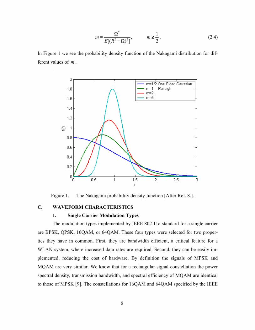
B. NAKAGAMI FADING MODEL The distribution we selected to model the fading channel is the Nakagami distri-
bution. The reason is its flexibility and accuracy in matching experimental data. Chang-
ing the m parameter of the distribution, we can model a wide variety of fading condi-
tions. The Rayleigh fading channel is a special case with 1m = , one-sided Gaussian fad-
ing is a special case with 1/ 2m = , and non-fading is a special case that occurs when m
approaches infinity.
The Nakagami- m density function is a function of two parameters, r and Ω , and
is given by [8] as:
2
2 12( )( )
m mrm
Rmf r r e
m−− Ω = Γ Ω
, (2.1)
where Ω is defined as
2[ ]E RΩ = . (2.2)
( )mΓ is the Gamma function defined as
1
0
( ) , 0m tm t e dt m∞
− −Γ = ≥∫ (2.3)
and the m parameter is expressed as
6
2
2 2
1,[( ) ] 2
m mE R
Ω= ≥− Ω
. (2.4)
In Figure 1 we see the probability density function of the Nakagami distribution for dif-
ferent values of m .
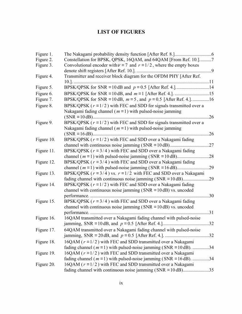
Figure 1. The Nakagami probability density function [After Ref. 8.].
C. WAVEFORM CHARACTERISTICS
1. Single Carrier Modulation Types The modulation types implemented by IEEE 802.11a standard for a single carrier
are BPSK, QPSK, 16QAM, or 64QAM. These four types were selected for two proper-
ties they have in common. First, they are bandwidth efficient, a critical feature for a
WLAN system, where increased data rates are required. Second, they can be easily im-
plemented, reducing the cost of hardware. By definition the signals of MPSK and
MQAM are very similar. We know that for a rectangular signal constellation the power
spectral density, transmission bandwidth, and spectral efficiency of MQAM are identical
to those of MPSK [9]. The constellations for 16QAM and 64QAM specified by the IEEE
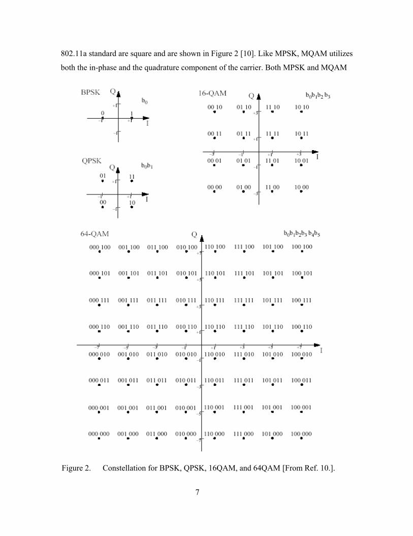
7
802.11a standard are square and are shown in Figure 2 [10]. Like MPSK, MQAM utilizes
both the in-phase and the quadrature component of the carrier. Both MPSK and MQAM
Figure 2. Constellation for BPSK, QPSK, 16QAM, and 64QAM [From Ref. 10.].
8
demodulate the two components of the carrier independently and can be thought of as
two independent M-ary pulse amplitude modulation (MPAM) signals. Due to this, it is
easy to implement a receiver for each of these modulation types using the same hardware.
In Chapters III and IV, we investigate the performance obtained with each of the modula-
tion types.
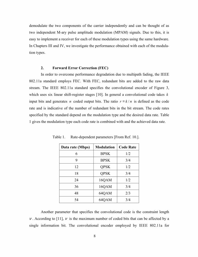
2. Forward Error Correction (FEC) In order to overcome performance degradation due to multipath fading, the IEEE
802.11a standard employs FEC. With FEC, redundant bits are added to the raw data
stream. The IEEE 802.11a standard specifies the convolutional encoder of Figure 3,
which uses six linear shift-register stages [10]. In general a convolutional code takes k
input bits and generates n coded output bits. The ratio /r k n= is defined as the code
rate and is indicative of the number of redundant bits in the bit stream. The code rates
specified by the standard depend on the modulation type and the desired data rate. Table
1 gives the modulation type each code rate is combined with and the achieved data rate.
Table 1. Rate-dependent parameters [From Ref. 10.].
Data rate (Mbps) Modulation Code Rate
6 BPSK 1/2
9 BPSK 3/4
12 QPSK 1/2
18 QPSK 3/4
24 16QAM 1/2
36 16QAM 3/4
48 64QAM 2/3
54 64QAM 3/4
Another parameter that specifies the convolutional code is the constraint length
ν . According to [11], ν is the maximum number of coded bits that can be affected by a
single information bit. The convolutional encoder employed by IEEE 802.11a for
9
1/ 2r = has a constraint length 7ν = and is shown in Figure 3. The less redundant code
rates of 2/3, and 3/4 are derived from it through puncturing. Puncturing implies that some
of the encoded bits are omitted so that the number of the transmitted bits is reduced, and
the code rate is increased. The omitted bits are replaced by dummy “zero” bits. These
dummy bits are accounted for by the decoder.
Figure 3. Convolutional encoder with 7ν = and 1/ 2r = , where the empty boxes denote shift registers [After Ref. 10.].
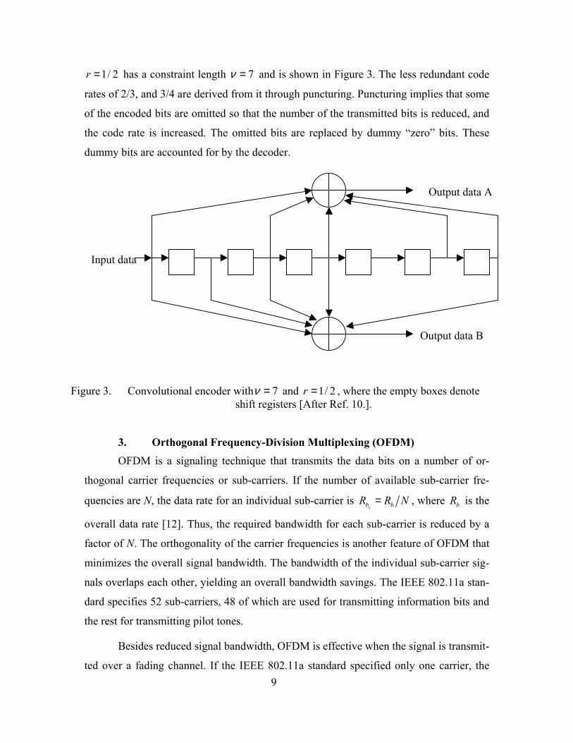
3. Orthogonal Frequency-Division Multiplexing (OFDM) OFDM is a signaling technique that transmits the data bits on a number of or-
thogonal carrier frequencies or sub-carriers. If the number of available sub-carrier fre-
quencies are N, the data rate for an individual sub-carrier is cb bR R N= , where bR is the
overall data rate [12]. Thus, the required bandwidth for each sub-carrier is reduced by a
factor of N. The orthogonality of the carrier frequencies is another feature of OFDM that
minimizes the overall signal bandwidth. The bandwidth of the individual sub-carrier sig-
nals overlaps each other, yielding an overall bandwidth savings. The IEEE 802.11a stan-
dard specifies 52 sub-carriers, 48 of which are used for transmitting information bits and
the rest for transmitting pilot tones.
Besides reduced signal bandwidth, OFDM is effective when the signal is transmit-
ted over a fading channel. If the IEEE 802.11a standard specified only one carrier, the
Input data
Output data A
Output data B
10
high data rate would cause the noise equivalent bandwidth (W ) of the signal to exceed
the coherence bandwidth of the channel ( )cf∆ [9]. In this case ( )cW f> ∆ , and the chan-
nel is said to be frequency-selective. As a result, the distortion of the signal is significant.
For each sub-carrier of an OFDM signal, the noise equivalent bandwidth cW is reduced
by N and is less than the coherence bandwidth of the channel ( )c cW W N f= < ∆ .
Hence, the channel is characterized as flat-fading for each individual sub-carrier.
While the use of N sub-carriers reduces the bandwidth, it increases bit duration
or symbol duration, depending on the modulation type, as:
cb bT NT= . (2.5)
If we let N get very large, the bit duration of each carrier may become larger than chan-
nel coherence time ( )cb cT t> ∆ , and the channel is then characterized as fast fading. In a
fast fading channel, the channel impulse response changes rapidly within the bit duration.
This causes frequency dispersion due to Doppler spreading, which leads to signal distor-
tion [13]. To avoid the latter, the channel must remain slowly fading and that limits the
maximum allowable value of N .
Figure 4 illustrates the generation of an OFDM signal, where we see the transmit-
ter and receiver block diagram. On the transmitter side, the information bits are first con-
volutionally encoded by the encoder of Figure 3. Then, a block interleaver, defined by a
two-step permutation, interleaves the coded bits. The first permutation ensures that adja-
cent coded bits are mapped onto nonadjacent sub-carriers. The second ensures that adja-
cent coded bits are mapped alternatively onto less and more significant bits of the con-
stellation of Figure 2 [10]. Spreading the bits over time prevents the important bits of a
block of source bits from being corrupted when there is a deep fade or noise burst.
After the interleaver stage, data are mapped. They are divided into groups of one,
two, four, or six bits and converted into complex numbers representing BPSK, QPSK,
16QAM, or 64QAM constellation points, respectively. The inverse fast Fourier transform
(IFFT) transforms these symbols into a complex baseband signal. The smoothness of the
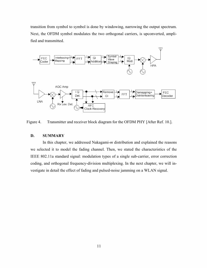
11
transition from symbol to symbol is done by windowing, narrowing the output spectrum.
Next, the OFDM symbol modulates the two orthogonal carriers, is upconverted, ampli-
fied and transmitted.
Figure 4. Transmitter and receiver block diagram for the OFDM PHY [After Ref. 10.].
D. SUMMARY In this chapter, we addressed Nakagami-m distribution and explained the reasons
we selected it to model the fading channel. Then, we stated the characteristics of the
IEEE 802.11a standard signal: modulation types of a single sub-carrier, error correction
coding, and orthogonal frequency-division multiplexing. In the next chapter, we will in-
vestigate in detail the effect of fading and pulsed-noise jamming on a WLAN signal.

12
THIS PAGE INTENTIONALLY LEFT BLANK
13
III. PERFORMANCE ANALYSIS WITH FEC AND SDD FOR SIGNALS TRANSMITTED OVER A NAKAGAMI FADING
CHANNEL WITH PULSED-NOISE JAMMING
A. INTRODUCTION In the previous chapter, we examined all the necessary background required to
understand the basic principles of the IEEE 802.11a wireless local area network standard.
Now it is time to see how these principles are applied in practice by proceeding to the
performance analysis. We examined the different modulation types separately for the
coded and uncoded case. In [3] and [4], whose work was continued in this thesis, the
analysis included the performance of coded signals, decoded with both hard decision de-
coding (HDD) and soft decision decoding (SDD). Since this thesis was concentrated
solely on the actual characteristics of the IEEE 802.11a wireless local area network stan-
dard, in addition to no coding, we examined only SDD. Especially for M-ary QAM, we
addressed specific assumptions made to analyze non-binary signals with SDD.
Lastly, we expanded our results to the combined OFDM signal and examined the
effect of fading when all 48 sub-carriers are considered one signal. In all cases we as-
sumed the signal experienced frequency-selective, slow Nakagami fading and pulsed-
noise jamming.
B. BPSK/QPSK These two modulation types were examined together since they are both analyzed
in the same way. A QPSK signal is a special case of M-ary PSK that enjoys double the
data rate of BPSK, since both the in-phase and the quadrature component of the carrier
are utilized.
1. Without SDD The material of this section has been derived in [4] and the probability of bit error
rate is restated here:
14
( )( )
/ 1 1
1 1
( 0.5)
1 SNR SIR / 12 ( 1) 1SNR SIR /
BPSK QPSKb mp mP
m pm
m pπ
− −
− −
Γ += + + Γ + + +
( ) 11 10 1
0.5 111 (SNR SIR / )
kk
k i
m im i m p
∞
−− −= =
+ − × + + + +
∑ ∏
0 1
1 ( 0.5) 0.5 11 SNRSNR 11 2 ( 1) 1SNR
k
k
mk i
p m m im im
m mmπ
∞
= =
− Γ + + − + + + + + Γ + +
∑ ∏ . (3.1)
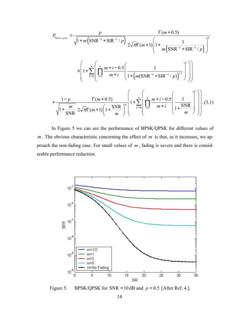
In Figure 5 we can see the performance of BPSK/QPSK for different values of
m . The obvious characteristic concerning the effect of m is that, as it increases, we ap-
proach the non-fading case. For small values of m , fading is severe and there is consid-
erable performance reduction.
Figure 5. BPSK/QPSK for SNR 10= dB and 0.5p = [After Ref. 4.].
15
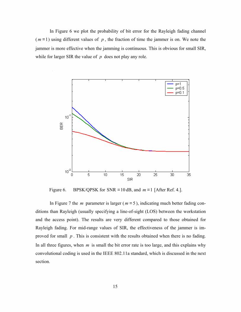
In Figure 6 we plot the probability of bit error for the Rayleigh fading channel
( 1m = ) using different values of p , the fraction of time the jammer is on. We note the
jammer is more effective when the jamming is continuous. This is obvious for small SIR,
while for larger SIR the value of p does not play any role.
Figure 6. BPSK/QPSK for SNR 10= dB, and 1m = [After Ref. 4.].
In Figure 7 the m parameter is larger ( 5m = ), indicating much better fading con-
ditions than Rayleigh (usually specifying a line-of-sight (LOS) between the workstation
and the access point). The results are very different compared to those obtained for
Rayleigh fading. For mid-range values of SIR, the effectiveness of the jammer is im-
proved for small p . This is consistent with the results obtained when there is no fading.
In all three figures, when m is small the bit error rate is too large, and this explains why
convolutional coding is used in the IEEE 802.11a standard, which is discussed in the next
section.
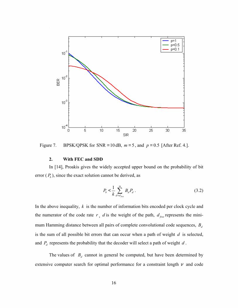
16
Figure 7. BPSK/QPSK for SNR 10= dB, 5m = , and 0.5p = [After Ref. 4.].
2. With FEC and SDD In [14], Proakis gives the widely accepted upper bound on the probability of bit
error ( bP ), since the exact solution cannot be derived, as
1
free
b d dd d
P B Pk
∞
=
< ∑ . (3.2)
In the above inequality, k is the number of information bits encoded per clock cycle and
the numerator of the code rate r , d is the weight of the path, freed represents the mini-
mum Hamming distance between all pairs of complete convolutional code sequences, dB
is the sum of all possible bit errors that can occur when a path of weight d is selected,
and dP represents the probability that the decoder will select a path of weight d .
The values of dB cannot in general be computed, but have been determined by
extensive computer search for optimal performance for a constraint length ν and code
17
rate r convolutional code. After [10], in Table 2 the values of dB are shown for the
codes specified by the IEEE 802.11a standard.
Table 2. Weight Structure of the Best Convolutional Codes [After Ref. 10.].
Code Rate freed freedB 1freedB + 2freedB + 3freedB + 4freedB +
1/2 10 36 0 211 0 1404
2/3 6 1 81 402 1487 6793
3/4 5 21 252 1903 11995 72115
According to [12], the sum in Inequality (3.2) is dominated by the first five non-zero
terms of the summation.
From this point on, the analysis diverges depending on whether we are dealing
with SDD or HDD. To continue with SDD, we expand the approach of [4] in order to ac-
commodate the case when the receiver has no information whether a bit is jammed or not.
Consequently, we have to find dP so as to be able to evaluate Inequality (3.2). For opti-
mum performance the use of a maximum-likelihood receiver is required. A maximum-
likelihood receiver maximizes the conditional probability density function of the received
code sequence ( | )rf r v given the correct code sequence v for equally likely code se-
quences. For the BPSK/QPSK signal, the output of the demodulator for each bit lr is
modeled as a Gaussian random variable with mean 2lcr a= and variance 2
lσ . If the cor-
rect path is the all-zero path and the thr path differs from the correct path in d bits, then
a decoding error occurs when [14]
21
0ld
c l
l l
a rσ=
>∑ . (3.3)
In the preceding equation the index l runs over the set of d bits in which the thr
path differs from the correct path, lr is the demodulator output, lca is the amplitude of
18
the received signal and is modeled as a random variable due to the effect of the fading
channel, and 2lσ is the power of the noise for each bit, which we must know in order to
distinguish between bits that are jammed and those that are not. The probability dP is
simply
21
0ld
c ld r
l l
a rP P
σ=
= >
∑ . (3.4)
We define
2lc l
ll
a rz
σ= . (3.5)
Obviously, after this transformation of random variables lz remains a Gaussian random
variable with mean 2 22ll c lz a σ= and variance 2 2
lc la σ . We now introduce z as the sum
of d independent random variables
1
d
ll
z z=
=∑ , (3.6)
where z is a Gaussian random variable since it is the summation of independent Gaussian
random variables. The mean of z is 2 2
12
l
d
c ll
z a σ=
= ∑ and the variance is 2 2
1l
d
c ll
a σ=∑ .
Combining Equations (3.4) and (3.6), we get
( 0)d rP P z= > . (3.7)
Expressing dP in terms of the Q-function, we can write
22
22 21
22 21
21
2
2
l
l
l
dc
dl l cd d
lcz l
l l
a
azP Q Q Qa
σ
σ σσ
=
=
=
= = =
∑∑
∑. (3.8)
19
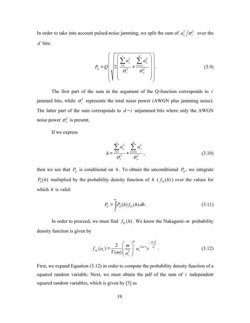
In order to take into account pulsed-noise jamming, we split the sum of 2 2lc la σ over the
d bits:
2 2
1 12 22
l l
i d
c cl l i
dt o
a aP Q
σ σ= = +
= +
∑ ∑. (3.9)
The first part of the sum in the argument of the Q-function corresponds to i
jammed bits, while 2tσ represents the total noise power (AWGN plus jamming noise).
The latter part of the sum corresponds to d i− unjammed bits where only the AWGN
noise power 2oσ is present.
If we express
2 2
1 12 2
l l
i d
c cl l i
t o
a ah
σ σ= = += +∑ ∑
, (3.10)
then we see that dP is conditional on h . To obtain the unconditional dP , we integrate
( )dP h multiplied by the probability density function of h ( ( )Hf h ) over the values for
which h is valid:
0
( ) ( )d d HP P h f h dh∞
= ∫ . (3.11)
In order to proceed, we must find ( )Hf h . We know the Nakagami- m probability
density function is given by
2
22 1
2
2( )( )
c
c
m m a
amAc c c
c
mf a a em a
−−
= Γ
. (3.12)
First, we expand Equation (3.12) in order to compute the probability density function of a
squared random variable. Next, we must obtain the pdf of the sum of i independent
squared random variables, which is given by [3] as
20
1
11
1( 1) 1( )
mi m bmi b
Bmf b b e
mi b−− = Γ
(3.13)
where the random variable 1b is defined as
2
11
l
i
cl
b a=
=∑ , (3.14)
and b is the average power of the signal. Analogously, the pdf of the sum of d i− inde-
pendent squared random variables is
( )
( ) 2( ) 1
21( 2) 2( )
m d i m bm d i b
Bmf b b e
m d i b
−−− − = Γ −
, (3.15)
where
2
12
l
d
cl i
b a= +
= ∑ . (3.16)
Substituting Equations (3.14) and (3.16) into Equation (3.10), we get
2 2
1 2 1 2t o
b bh h hσ σ
= + = + . (3.17)
Next, we must find the pdfs of 1h and 2h . From Equation (3.17),
22
1 11 ,1 t
t
b dbhdh
σσ
= = . (3.18)
We know that
11 1 1 ( 1)
| 1|( 1) ( 1) || 1|H B b f h
dbf h f bdh −=
= (3.19)
Substituting Equations (3.13) and (3.18) into Equation (3.19), we get
2 1
2 11
1( 1) ( ) 1( )
tmi m h
mi mi bH t
mf h h emi b
σ
σ−− = Γ
. (3.20)
21
Following the same methodology, we obtain the pdf of 2h as
( )
2( ) 22 ( ) ( ) 1
21( 2) ( ) 2( )
om d i m h
m d i m d i bH o
mf h h em d i b
σ
σ−
−− − − = Γ − . (3.21)
The last step is to find the pdf of the sum of 1 2h h+ . It is given by the convolu-
tion of the two separate pdfs. However, we will take advantage of the relevant property of
the Laplace transformation, stating that convolution is equivalent to multiplication in the
Laplace domain. Thus, we multiply the two pdfs after their transformation into the
Laplace domain. Since the pdf is non-zero only for positive arguments,
11 1 1
0
( 1) ( ) ( 1) 1shH H Hf h F s f h e dh
∞−= = ∫L (3.22)
where iL indicates the Laplace transform operator. Substituting Equation (3.20) into
(3.22), we get
2 1
2 1 11
0
1( ) ( ) 1 1( )
tmi m h
mi mi shbH t
mF s h e e dhmi b
σ
σ∞
−− − = Γ ∫ (3.23)
which can be simplified to
21
2 11
0
1( ) ( ) 1 1( )
tmmi s hbmi mi
H tmF s h e dhb mi
σ
σ ∞ − + − = Γ
∫ . (3.24)
Using the Laplace transform pair
1 1
( ) ( )
uat
u
t eu s a
−−
= Γ + L for 0u > , (3.25)
we set
1ct h= , (3.26)
u mi= , (3.27)
and
2t
c
ma sbσ= + , (3.28)
22
which allows us to get
21 2
1( ) ( )mi
miH t mi
t
mF sb ms
b
σσ
= +
. (3.29)
Similarly,
22 2 2
0
( 2) ( ) ( 2) 2shH H Hf h F s f h e dh
∞−= = ∫L (3.30)
which can be evaluated to yield
( )
2 ( )2 ( )2
1( ) ( )m d i
m d iH o m d i
o
mF sb ms
b
σσ
−−
−
= +
. (3.31)
The pdf of h in the Laplace domain is the product of 1( 1)Hf hL and 2 ( 2)Hf hL :
1 2( ) ( ) ( 1) ( 2)H H H Hf h F s f h f h= =L L L . (3.32)
Hence, substituting Equations (3.29) and (3.31) into Equation (3.32), we get
( )
2 2 ( )( )2 2
1 1( ) ( ) ( )mi m d i
mi m d iH t omi m d i
t o
m mF sb bm ms s
b b
σ σσ σ
−−
−
= + +
(3.33)
which can be simplified to
2 2 ( )
( )2 2
( ) ( )( )md mi m d i
t oH mi m d i
t o
mF sb m ms s
b b
σ σσ σ
−
−
= + +
. (3.34)
To write Equation (3.34) in terms of SNR and SIR we define
2SNRo
bσ
= (3.35)
and
2SIRj
bσ
= , (3.36)
23
where 2oσ is the power of the AWGN and 2
jσ is the noise power of the jamming signal.
Combining both powers, we get the total power
2 2 2t o jσ σ σ= + . (3.37)
The resulting signal-to-noise plus interference ratio is
22 2 2 2
1SNIRjt o j o
b b
b bσσ σ σ σ
= = =+
+ (3.38)
which can be written
( ) 11 11 1
1SNIR SNR SIRSNR SIR
−− −− −= = +
+. (3.39)
Now we can rewrite Equation (3.34) as
( )
( )
1 1 ( )
( )
11 1
SNR SIR SNR( )
SNRSNR SIR
c
mi m d i md
H mim d i
mF s
m ms s
− − − −
−
−− −
+=
+ + +
. (3.40)
The inverse Laplace transform of the equation above is too complicated to calcu-
late directly. Alternatively, we use the methodology [9] of the numerical inverse of the
two-sided Laplace transform. The latter is defined as
( ) ( ) ( ) sxX X Xf x F s f x e dx
∞−
−∞
= = ∫L . (3.41)
The inverse two-sided Laplace transform is given by
1( ) ( ) ( )2
c jsx
X X Xc j
F s f x F s e dsjπ
+ ∞
− ∞
= = ∫-1L . (3.42)
where c must be within the strip of convergence of ( )XF s [9]. By successive changes of
variables we get
24
/ 2
0
( ) Re ( tan ) cos( tan )cx
X Xcef x F c jc cx
π
φ φπ
= +∫
2Im ( tan ) sin( tan ) secXF c jc cx dφ φ φ φ− + . (3.43)
Rewriting Equation (3.43) in terms of the notation used, we have
/ 2
0
( ) Re ( tan ) cos( tan )cx
H Hcef h F c jc cx
π
φ φπ
= +∫
2Im ( tan ) sin( tan ) secHF c jc cx dφ φ φ φ− + . (3.44)
Up to this point we have evaluated ( )dP i . Next, we find dP independent of i . The
probability of selecting a path that is a Hamming distance d from the correct path when
i of the d bits are jammed for BPSK/QPSK is the sum of the probability that one bit is
jammed and 1d − are not, plus the probability of two bits are jammed and 2d − are not,
etc., and is expressed as
0
( bits jammed) ( )d
d r di
P P i P i=
=∑ , (3.45)
where ( )dP i is found by substituting Equation (3.44) in Equation (3.11). The probability
( bits jammed)rP i is
( bits jammed) (1 )i d ir
dP i p p
i−
= −
. (3.46)
where p is the fraction of time the jammer is on. Now Equation (3.45) is written as
0
(1 ) ( )d
i d id d
i
dP p p P i
i−
=
= −
∑ . (3.47)
We have almost concluded the analysis, but we must take into account two more
things. The first is the assumption that the average jamming power remains constant, in-
dependent of p . This statement implies that instantaneous jamming power increases
when the jammer is on. Thus, SIR is replaced with
25
SIRSIRp
′ = . (3.48)
The second thing is the relation between the average energy of the uncoded data
bit bE and the coded onecbE . The uncoded data rate bR is r times the coded data rate
cbR ,
cb bR rR= . (3.49)
In addition, the average transmitted power is the same whether coded or uncoded bits are
transmitted. Hence,
c cb b b bP E R E R= = (3.50)
and
c
c
bb b b
b
RE E rER
= = . (3.51)
This means that the power of coded bits is r times the power of uncoded bits. To com-
pensate for this, we must multiply the expressions for uncoded bit power (SNR and SIR)
by the code rate r .
In light of Equation (3.47) and the considerations of the previous two paragraphs,
we can now numerically evaluate Equation (3.11). With the values in Table 2 for dB , we
can then calculate Equation (3.2). For the code rate 1/ 2r = , which is used for data rates
of six Mbps (BPSK) and 12 Mbps (QPSK), we get Figures 8 and 9 for different values of
SNR (10 dB and 16 dB, respectively). The points of interest in the Figures are, firstly, the
fact that as SIR increases the probability of error converges to the value corresponding to
no jamming. Second, it is obvious that the jamming signal is far more efficient when em-
ploying continuous jamming ( 1p = ).
Taking as a reference the performance for 410bP −= , the comparison between the
curves for 1p = and 0.5p = yields a difference of seven dB for SNR 10= dB. What is
more, the performance for 0.1p = is small even for small values of SIR. Undoubtedly,
maximum-likelihood detection with SDD deprives the jammer of using pulsed-noise
techniques. Pulsed-noise jamming techniques are preferred when attacking a communi-
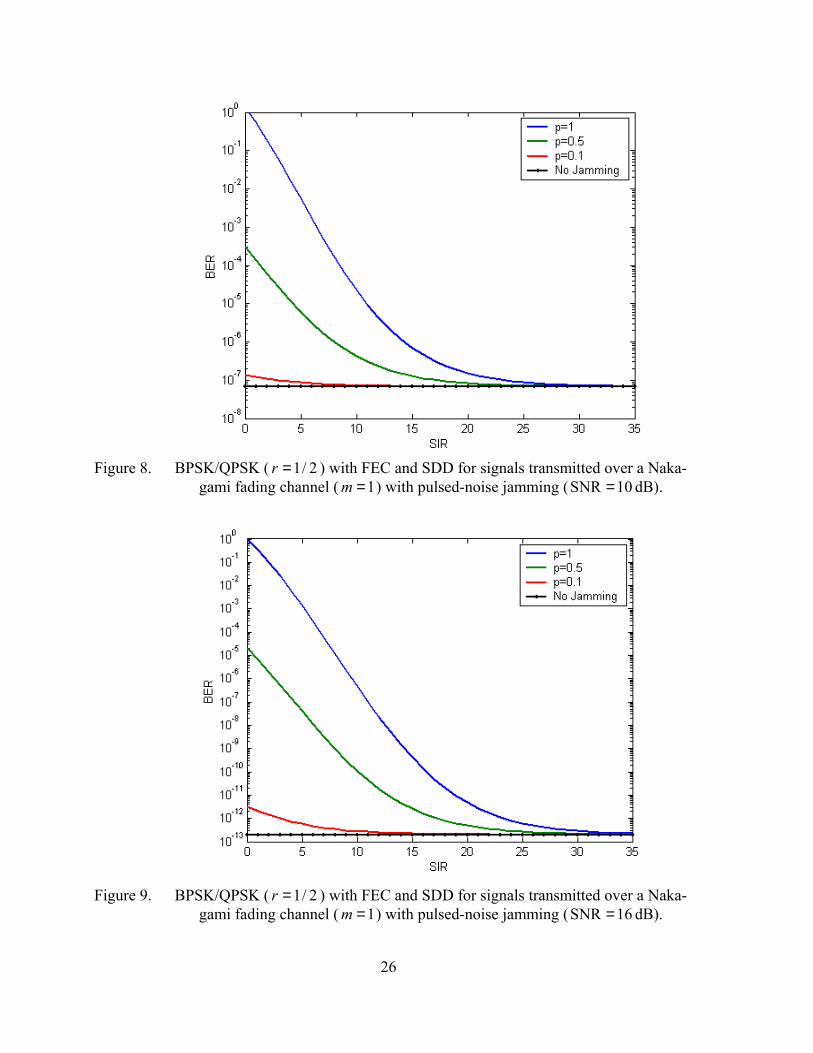
26
Figure 8. BPSK/QPSK ( 1/ 2r = ) with FEC and SDD for signals transmitted over a Naka-
gami fading channel ( 1m = ) with pulsed-noise jamming (SNR 10= dB).
Figure 9. BPSK/QPSK ( 1/ 2r = ) with FEC and SDD for signals transmitted over a Naka-
gami fading channel ( 1m = ) with pulsed-noise jamming (SNR 16= dB).
27
cation system not employing FEC and SDD, as was shown in Figure 7. However, for the
IEEE 802.11a wireless local area network standard, FEC with SDD is specified.
To examine the effect of the Nakagami fading channel, we examine Figure 10,
which demonstrates system performance for different values of the m parameter. Based
on the findings from the two previous figures, where the worst-case scenario for the re-
ceiver is for 1p = , we plot the probability of bit error only for continuous noise jamming.
Initially, we observe that, as m increases, the performance of the receiver improves. As
m approaches infinity, the performance approaches the AWGN limit. The difference in
performance for small values of SIR is minor. In other words, when the jamming power
is large, the fading conditions play a minor role. Conversely, as SIR increases and we en-
counter small jamming power, the results are the opposite. For large SIR, the fading con-
ditions determine to a large extent the overall performance. A small increase of m from
1/2 to 1 improves the bit error rate by a magnitude of 310− when SNR 10= dB.
Figure 10. BPSK/QPSK ( 1/ 2r = ) with FEC and SDD over a Nakagami fading channel with
continuous noise jamming (SNR 10= dB).
28
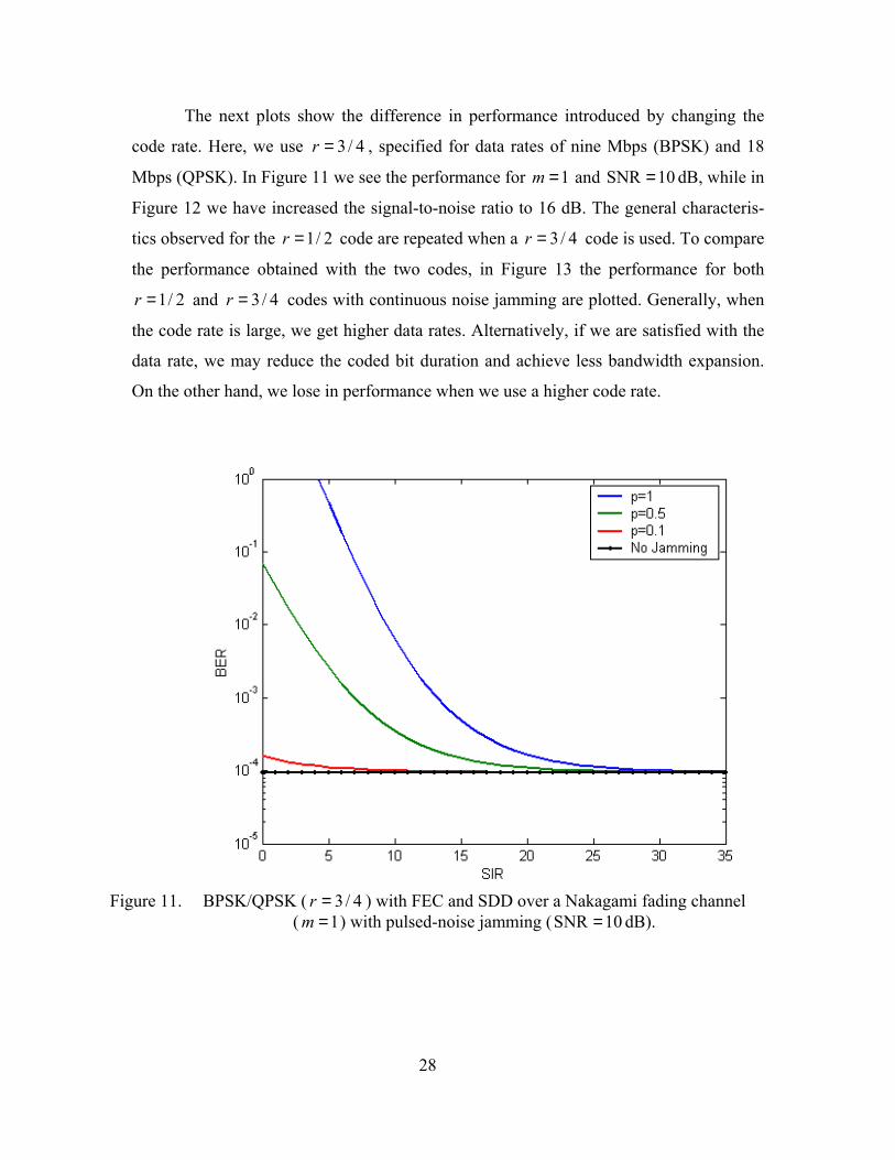
The next plots show the difference in performance introduced by changing the
code rate. Here, we use 3 / 4r = , specified for data rates of nine Mbps (BPSK) and 18
Mbps (QPSK). In Figure 11 we see the performance for 1m = and SNR 10= dB, while in
Figure 12 we have increased the signal-to-noise ratio to 16 dB. The general characteris-
tics observed for the 1/ 2r = code are repeated when a 3 / 4r = code is used. To compare
the performance obtained with the two codes, in Figure 13 the performance for both
1/ 2r = and 3 / 4r = codes with continuous noise jamming are plotted. Generally, when
the code rate is large, we get higher data rates. Alternatively, if we are satisfied with the
data rate, we may reduce the coded bit duration and achieve less bandwidth expansion.
On the other hand, we lose in performance when we use a higher code rate.
Figure 11. BPSK/QPSK ( 3 / 4r = ) with FEC and SDD over a Nakagami fading channel
( 1m = ) with pulsed-noise jamming (SNR 10= dB).

29
Figure 12. BPSK/QPSK ( 3 / 4r = ) with FEC and SDD over a Nakagami fading channel
( 1m = ) with pulsed-noise jamming (SNR 16= dB).
Figure 13. BPSK/QPSK ( 3 / 4r = ) vs. 1/ 2r = with FEC and SDD over a Nakagami fading channel with continuous noise jamming (SNR 10= dB).
30
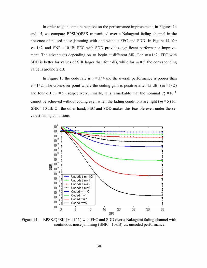
In order to gain some perceptive on the performance improvement, in Figures 14
and 15, we compare BPSK/QPSK transmitted over a Nakagami fading channel in the
presence of pulsed-noise jamming with and without FEC and SDD. In Figure 14, for
1/ 2r = and SNR 10= dB, FEC with SDD provides significant performance improve-
ment. The advantages depending on m begin at different SIR. For 1/ 2m = , FEC with
SDD is better for values of SIR larger than four dB, while for 5m = the corresponding
value is around 2 dB.
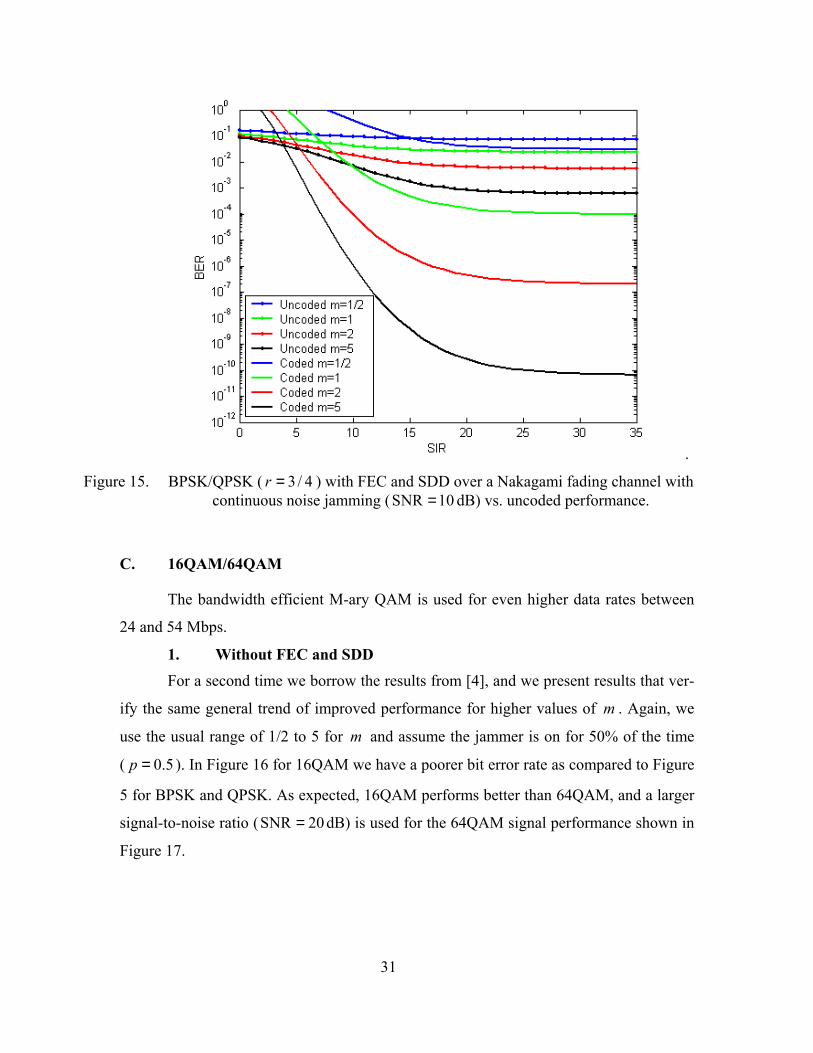
In Figure 15 the code rate is 3 / 4r = and the overall performance is poorer than
1/ 2r = . The cross-over point where the coding gain is positive after 15 dB ( 1/ 2m = )
and four dB ( 5m = ), respectively. Finally, it is remarkable that the nominal 410bP −=
cannot be achieved without coding even when the fading conditions are light ( 5m = ) for
SNR 10= dB. On the other hand, FEC and SDD makes this feasible even under the se-
verest fading conditions.
Figure 14. BPSK/QPSK ( 1/ 2r = ) with FEC and SDD over a Nakagami fading channel with
continuous noise jamming (SNR 10= dB) vs. uncoded performance.
31
.
Figure 15. BPSK/QPSK ( 3 / 4r = ) with FEC and SDD over a Nakagami fading channel with continuous noise jamming (SNR 10= dB) vs. uncoded performance.
C. 16QAM/64QAM
The bandwidth efficient M-ary QAM is used for even higher data rates between
24 and 54 Mbps.
1. Without FEC and SDD For a second time we borrow the results from [4], and we present results that ver-
ify the same general trend of improved performance for higher values of m . Again, we
use the usual range of 1/2 to 5 for m and assume the jammer is on for 50% of the time
( 0.5p = ). In Figure 16 for 16QAM we have a poorer bit error rate as compared to Figure
5 for BPSK and QPSK. As expected, 16QAM performs better than 64QAM, and a larger
signal-to-noise ratio (SNR 20= dB) is used for the 64QAM signal performance shown in
Figure 17.
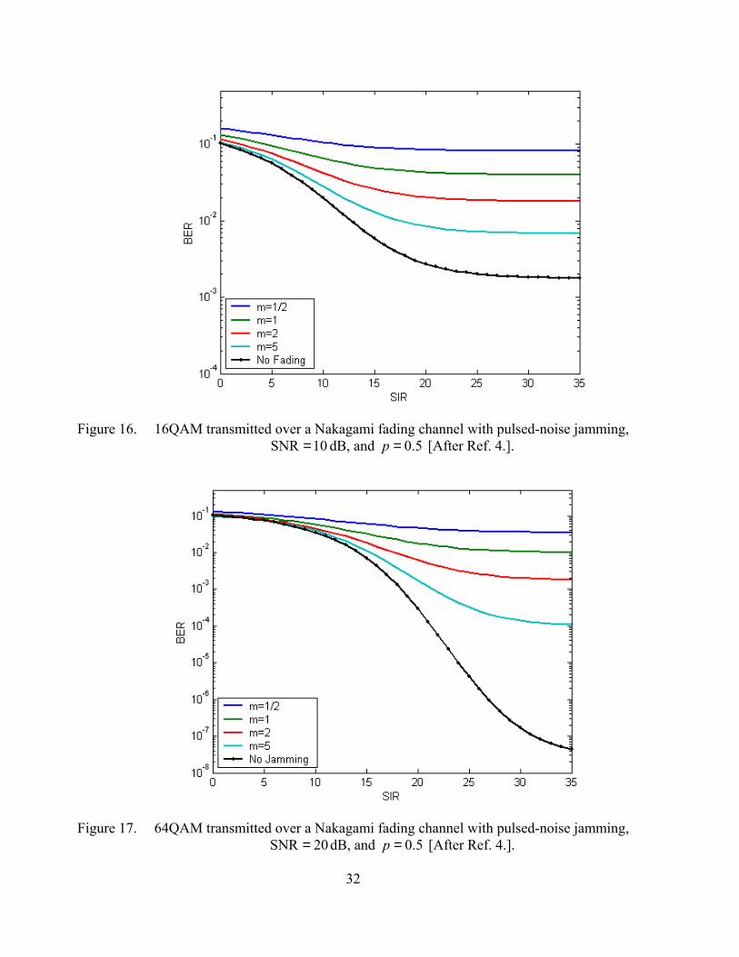
32
Figure 16. 16QAM transmitted over a Nakagami fading channel with pulsed-noise jamming,
SNR 10= dB, and 0.5p = [After Ref. 4.].
Figure 17. 64QAM transmitted over a Nakagami fading channel with pulsed-noise jamming,
SNR 20= dB, and 0.5p = [After Ref. 4.].
33
2. With FEC and SDD
The approach followed for the SDD demodulation for BPSK with FEC does not
apply for the MQAM case. Demodulating a binary signal with SDD means that the de-
modulator output is non-binary. Using a metric that provides enough resolution to sepa-
rate the various levels, like the Euclidean distance, the decoder decides which path is cor-
rect. When non-binary modulation is used, we cannot do the same. As a result, we as-
sume that the quantization is applied to the demodulated symbols. During the conversion
from symbol to bit, the resulting bits inherit the quantized level of the parent symbol.
Moreover, the process of deinterleaving spreads the bits in time, and we can reasonably
continue our analysis based on the approach for binary signals.
The main difference we should bear in mind is to use the proper formula for the
probability of bit error for M-ary QAM in Equation (3.9). According to [9], the probabil-
ity of bit error in AWGN for square M-ary QAM constellations is
4( 1) 3 SNR1b
M qP QMq M
−= − , (3.52)
where q is the number of bits per symbol, and M is the number of possible combina-
tions of q bits. The relation between q and M is 2logq M= . By analogy with Equation
(3.9), valid for BPSK with FEC and SDD, we get
2 2 2 2
1 1
34( 1)
1
l l
i d
c t c ol l i
d
q a aMP Q
Mq M
σ σ= = +
+ − = −
∑ ∑. (3.53)
Following the methodology used for BPSK and setting 16M = and 4q = , we get
Figures 18, 19, and 20 for 16QAM. In Figures 18 and 19 the signal experiences Rayleigh
fading for different values of p . Next, in Figure 20 the jamming is continuous, and we
again use the range for m (1/2, 5). As expected, the performance is worse than for
BPSK, but now data rate is higher. For 1/ 2r = with 16QAM, we have 24 Mbps, while
for 3 / 4r = with 16QAM, we get 36 Mbps.
34
Figure 18. 16QAM ( 1/ 2r = ) with FEC and SDD transmitted over a Nakagami fading chan-
nel ( 1m = ) with pulsed-noise jamming (SNR 10= dB).
Figure 19. 16QAM ( 1/ 2r = ) with FEC and SDD transmitted over a Nakagami fading chan-
nel ( 1m = ) with pulsed-noise jamming (SNR 16= dB).
35
Figure 20. 16QAM ( 1/ 2r = ) with FEC and SDD transmitted over a Nakagami fading chan-
nel with continuous noise jamming (SNR 10= dB).
The necessary alterations of Equation (3.53) for 64QAM, the last modulation
technique we are examining, is to set 64M = and 6q = . Again, we achieve higher data
rates, but the performance is even worse compared to all previous cases. For 2 / 3r =
with 64QAM we have 48 Mbps, while for 3 / 4r = with 64QAM we get 54 Mbps. In
Figure 21 we see the probability of bit error for 3 / 4r = . The combination of 64QAM
and the larger value of the possible code rates has the poorest performance and will be
used only in very favorable conditions of fading and signal-to-noise ratio. That is the rea-
son we use the relatively high value of SNR 26= dB.
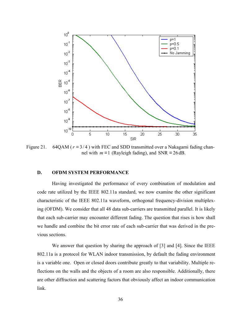
36
Figure 21. 64QAM ( 3/ 4r = ) with FEC and SDD transmitted over a Nakagami fading chan-
nel with 1m = (Rayleigh fading), and SNR 26= dB.
D. OFDM SYSTEM PERFORMANCE
Having investigated the performance of every combination of modulation and
code rate utilized by the IEEE 802.11a standard, we now examine the other significant
characteristic of the IEEE 802.11a waveform, orthogonal frequency-division multiplex-
ing (OFDM). We consider that all 48 data sub-carriers are transmitted parallel. It is likely
that each sub-carrier may encounter different fading. The question that rises is how shall
we handle and combine the bit error rate of each sub-carrier that was derived in the pre-
vious sections.
We answer that question by sharing the approach of [3] and [4]. Since the IEEE
802.11a is a protocol for WLAN indoor transmission, by default the fading environment
is a variable one. Open or closed doors contribute greatly to that variability. Multiple re-
flections on the walls and the objects of a room are also responsible. Additionally, there
are other diffraction and scattering factors that obviously affect an indoor communication
link.
37
The Nakagami distribution is a great aide in our effort, because by changing the
m parameter we model different fading channels. Supposing that both severe and mild
fading conditions are likely to occur simultaneously for different sub-carriers, we treat
each sub-carrier as being independent and subject to Nakagami fading with different m .
Assuming that all values of m are probable in a specific range, we model m as a uni-
formly distributed random variable. Ranging m from 1/2 to 5 is a reasonable assumption,
and we must calculate the bit error rate 48 times and take the average.
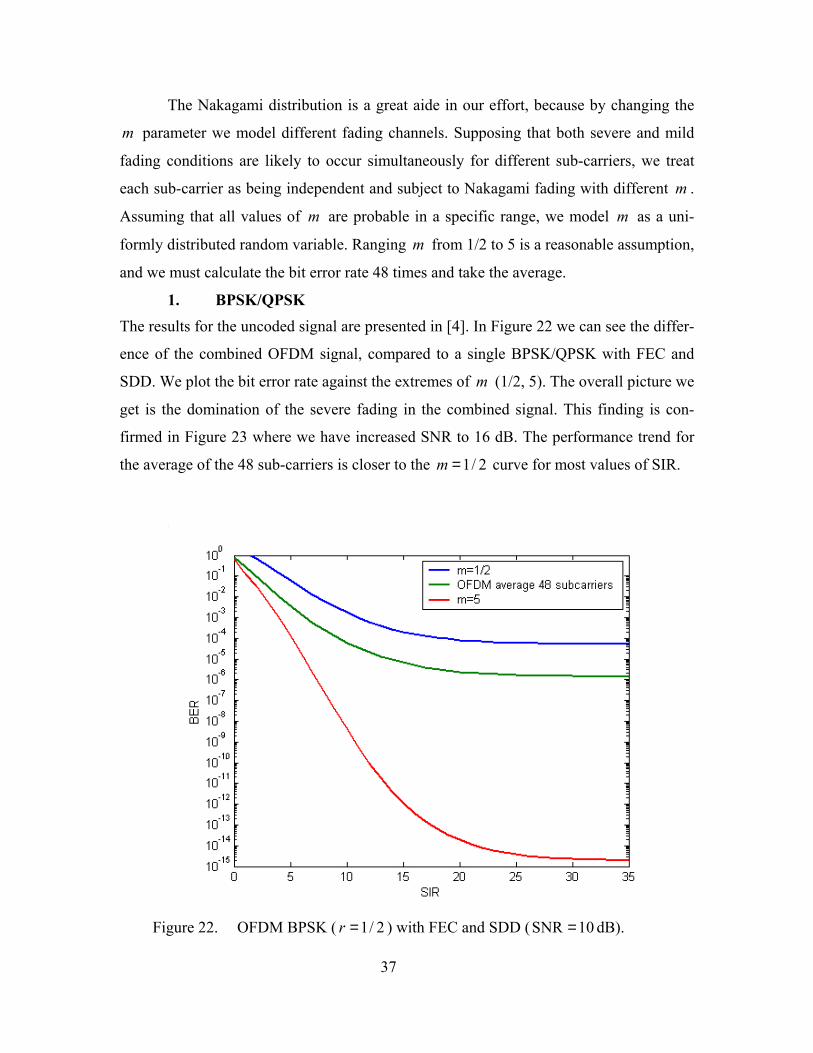
1. BPSK/QPSK The results for the uncoded signal are presented in [4]. In Figure 22 we can see the differ-
ence of the combined OFDM signal, compared to a single BPSK/QPSK with FEC and
SDD. We plot the bit error rate against the extremes of m (1/2, 5). The overall picture we
get is the domination of the severe fading in the combined signal. This finding is con-
firmed in Figure 23 where we have increased SNR to 16 dB. The performance trend for
the average of the 48 sub-carriers is closer to the 1/ 2m = curve for most values of SIR.
Figure 22. OFDM BPSK ( 1/ 2r = ) with FEC and SDD (SNR 10= dB).
38
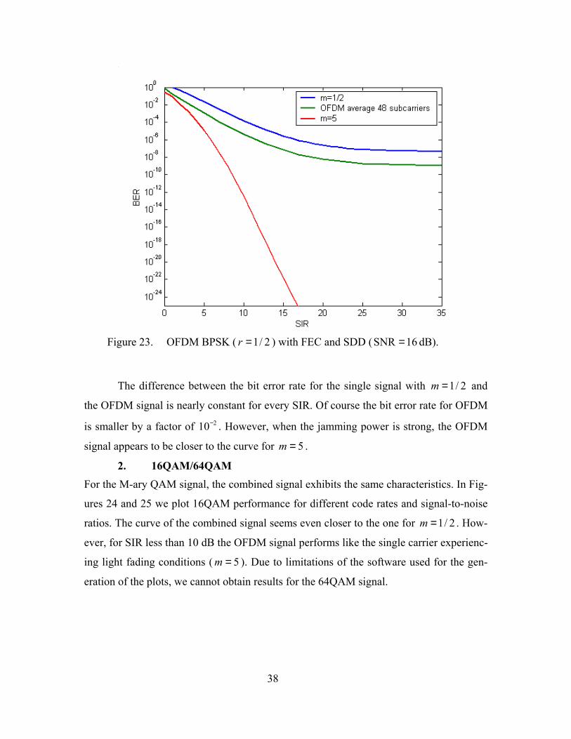
Figure 23. OFDM BPSK ( 1/ 2r = ) with FEC and SDD (SNR 16= dB).
The difference between the bit error rate for the single signal with 1/ 2m = and
the OFDM signal is nearly constant for every SIR. Of course the bit error rate for OFDM
is smaller by a factor of 210− . However, when the jamming power is strong, the OFDM
signal appears to be closer to the curve for 5m = .
2. 16QAM/64QAM For the M-ary QAM signal, the combined signal exhibits the same characteristics. In Fig-
ures 24 and 25 we plot 16QAM performance for different code rates and signal-to-noise
ratios. The curve of the combined signal seems even closer to the one for 1/ 2m = . How-
ever, for SIR less than 10 dB the OFDM signal performs like the single carrier experienc-
ing light fading conditions ( 5m = ). Due to limitations of the software used for the gen-
eration of the plots, we cannot obtain results for the 64QAM signal.
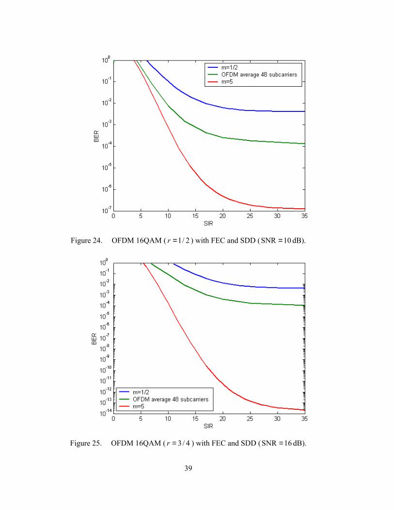
39
Figure 24. OFDM 16QAM ( 1/ 2r = ) with FEC and SDD (SNR 10= dB).
Figure 25. OFDM 16QAM ( 3/ 4r = ) with FEC and SDD (SNR 16= dB).
40
E. SUMMARY
This chapter presented the effect of fading and pulsed-noise jamming on the sig-
nal. The comparison between coded and uncoded performance is essential to establish the
importance of convolutional coding to reliable communication. We plotted the results for
various combinations of modulations and code rates. As the code rate increases, which
means that the coded signal has less redundancy, we confirmed the results of [4] regard-
ing the deterioration of the bit error rate. By changing parameter p , we determined that
continuous jamming is most effective against FEC and SDD for the maximum-likelihood
receiver. Variations of the m parameter gave insight as to how severe the effect of fading
is for 1/ 2m = compared to larger values of m .
In the last part, we dealt with the combined OFDM signal with FEC and SDD.
Based on the assumption that all sub-carriers are likely to experience different fading
conditions, we randomly assigned values for m in the region 1/2 to 5. For all modula-
tions the domination of the smallest m was obvious, which agreed with the findings for
uncoded OFDM after Ref [4].
Up to this point we have assumed the jamming signal does not experience any
kind of fading. This is close to reality for an airborne jammer who enjoys LOS with the
jammed receiver. The question that rises is what is the effect when the jammer does en-
counter fading, and this is discussed in the next chapter.
41
IV. PERFORMANCE ANALYSIS WITH FEC AND SDD, NAKAGAMI FADING CHANNELS, AND FADED PULSED-NOISE
JAMMING
A. INTRODUCTION Having examined the performance of a system designed to receive an IEEE
802.11a waveform transmitted over a Nakagami fading channel with pulsed-noise jam-
ming, we now proceed to evaluate the communications system performance when the
jamming signal also experiences fading. In this case the noise power of the jammer 2jσ is
no longer constant but must be modeled as a random variable. The probability of bit error
is now conditional on the noise power of the jammer. Since we assume a Nakagami fad-
ing channel, 2jσ is modeled as a Nakagami-squared random variable. This chapter is or-
ganized like the previous one in order to make comparison with previous results easier.
B. BPSK/QPSK
1. Without FEC In [14] the probability bit error for BPSK/QPSK with noise jamming is given as
2
2 22 cb
j o
aP Qσ σ
= +
(4.1)
where 2 2j oσ σ+ represents the power of additive, Gaussian noise. As mentioned previ-
ously, 2jσ is modeled as a random variable. As a result, Equation (4.1) is now a condi-
tional probability. To get the unconditional bP , we first need to find the pdf correspond-
ing to the argument of the Q-function, ( )2 2 2c j oa σ σ+ . This pdf is extremely complex
and, in order to simplify the analysis, we assume that the power of the AWGN 2oσ is neg-
ligible compared to 2jσ . This is true for most values of SIR when SNR is large. Now the
probability of bit error simplifies to

42
2
22 cb
j
aP Qσ
=
. (4.2)
To continue our analysis, we define
2
2c
j
a xtyσ
= = , (4.3)
which means that bP is now conditional on the random variable t
)(( ) 2bP t Q t= . (4.4)
Both x and y are independent, Nakagami-squared random variables and, by using the
pdf of a Nakagami-squared random variable obtained in [3] and adjusting it for our nota-
tion, we have
11( )( )
s ss
m m xms x
Xs
mf x x em x
−− = Γ (4.5)
11( )( )
j j
j
m m ymj y
Yj
mf y y e
m y
−− = Γ
(4.6)
where x is the average power of the received information signal, and y is the average
power of the jamming signal. The new parameters sm and jm are the Nakagami parame-
ters for the fading channel of the desired and the jamming signal, respectively.
As we find in [15], the pdf of the ratio of two independent random variables is
given by
0
( ) ( ) ( )T X Yf t y f t y f y dy∞
= ∫ . (4.7)
If we substitute Equations (4.5) and (4.6) into Equation (4.7), we get
( ) 1 1
0
1 1( )( ) ( )
j js ss j
m m ym m tym mj ys x
Ts j
mmf t y t y e y e dym x m y
∞ −−− − = Γ Γ ∫ (4.8)
43
which can be manipulated to give
11
0
1( )( ) ( )
j jss
s js
m mm tm ym m x yj ms
Ts j
mmf t t y e dym m x y
∞ − + + −− = Γ Γ
∫ . (4.9)
From [16] we use the identity
1
0
1 ( ), Re( ) 0, Re( ) 0xx e dxν µν ν µ ν
µ
∞− − = Γ > >∫ . (4.10)
Setting
s jm mν = + (4.11)
and
js mm tx y
µ = + , (4.12)
we can use (4.10) to evaluate (4.9) with the result
11 1( ) ( )( ) ( )
js
s
s j
mmj ms
T s jm ms j js
mmf t t m mm m x y mm t
x y
−+
= Γ + Γ Γ +
. (4.13)
Rearranging terms and expressing the second part in terms of SIR, where
SIR xy
= , (4.14)
we obtain to the pdf of the ratio of two Nakagami-squared random variables as
1( ) SIR( )( ) ( )
SIR
sj
s
s j
m ms j ms
T m ms j j
s
j
m m mf t tm m m m t
m
−+
Γ += Γ Γ +
. (4.15)
An alternative derivation of Equation (4.15) is given in [6].
To obtain the unconditional bP , we must integrate the product of the conditional
( )bP t and the probability density function ( )Tf t over the values for which t is valid:
44
0
( ) ( )b b TP P t f t dt∞
= ∫ . (4.16)
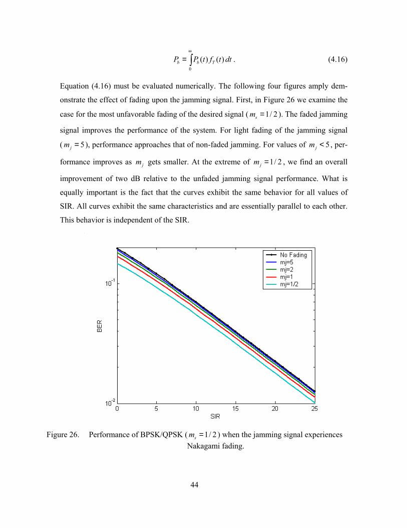
Equation (4.16) must be evaluated numerically. The following four figures amply dem-
onstrate the effect of fading upon the jamming signal. First, in Figure 26 we examine the
case for the most unfavorable fading of the desired signal ( 1/ 2sm = ). The faded jamming
signal improves the performance of the system. For light fading of the jamming signal
( 5jm = ), performance approaches that of non-faded jamming. For values of 5jm < , per-
formance improves as jm gets smaller. At the extreme of 1/ 2jm = , we find an overall
improvement of two dB relative to the unfaded jamming signal performance. What is
equally important is the fact that the curves exhibit the same behavior for all values of
SIR. All curves exhibit the same characteristics and are essentially parallel to each other.
This behavior is independent of the SIR.
Figure 26. Performance of BPSK/QPSK ( 1/ 2sm = ) when the jamming signal experiences
Nakagami fading.
45
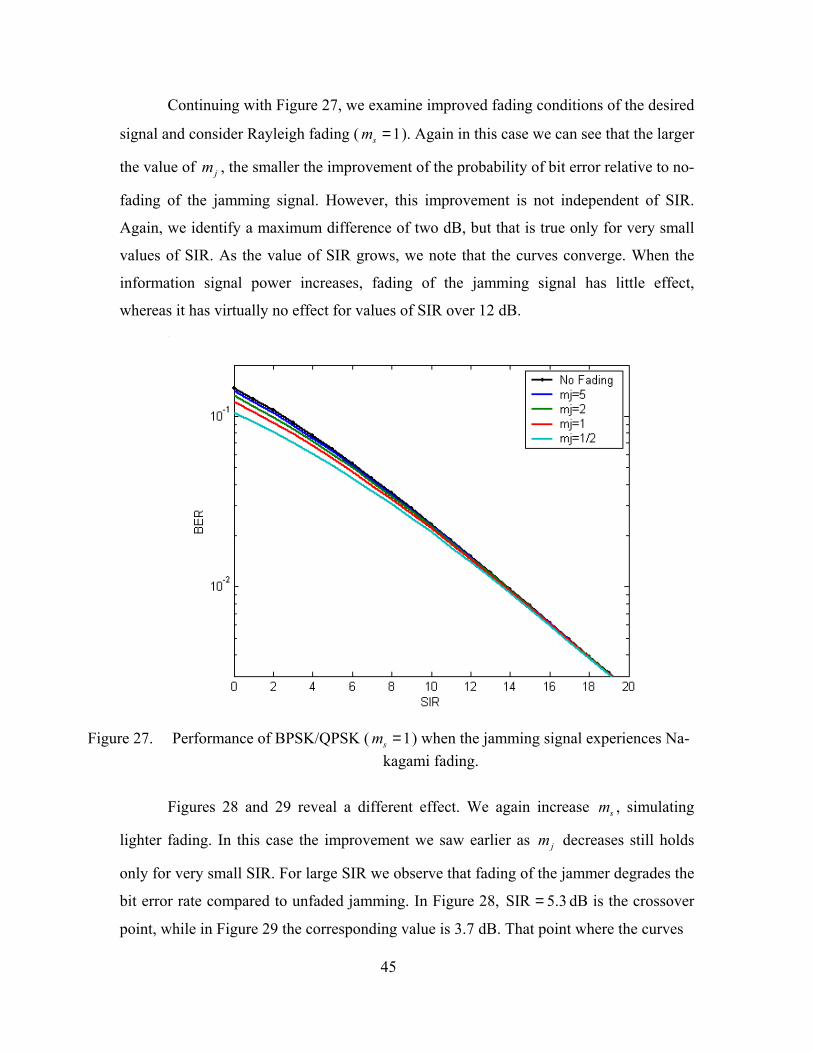
Continuing with Figure 27, we examine improved fading conditions of the desired
signal and consider Rayleigh fading ( 1sm = ). Again in this case we can see that the larger
the value of jm , the smaller the improvement of the probability of bit error relative to no-
fading of the jamming signal. However, this improvement is not independent of SIR.
Again, we identify a maximum difference of two dB, but that is true only for very small
values of SIR. As the value of SIR grows, we note that the curves converge. When the
information signal power increases, fading of the jamming signal has little effect,
whereas it has virtually no effect for values of SIR over 12 dB.
Figure 27. Performance of BPSK/QPSK ( 1sm = ) when the jamming signal experiences Na-
kagami fading.
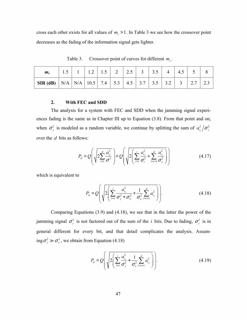
Figures 28 and 29 reveal a different effect. We again increase sm , simulating
lighter fading. In this case the improvement we saw earlier as jm decreases still holds
only for very small SIR. For large SIR we observe that fading of the jammer degrades the
bit error rate compared to unfaded jamming. In Figure 28, SIR 5.3= dB is the crossover
point, while in Figure 29 the corresponding value is 3.7 dB. That point where the curves
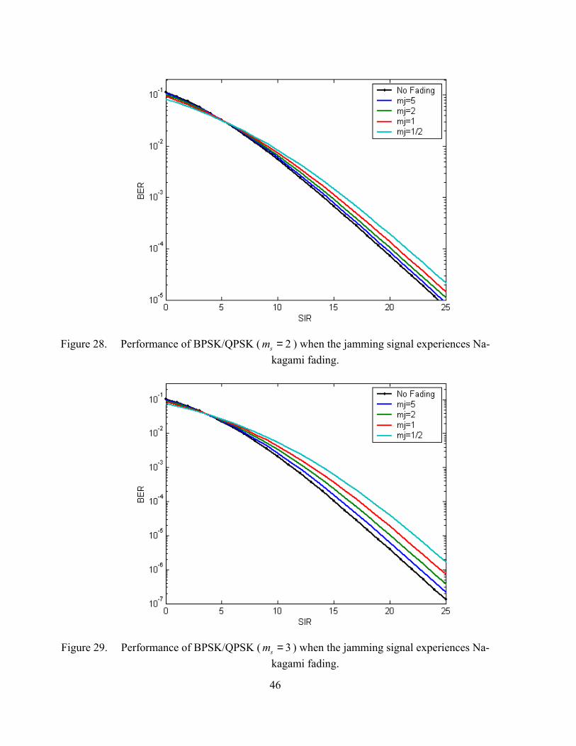
46
Figure 28. Performance of BPSK/QPSK ( 2sm = ) when the jamming signal experiences Na-
kagami fading.
Figure 29. Performance of BPSK/QPSK ( 3sm = ) when the jamming signal experiences Na-
kagami fading.
47
cross each other exists for all values of 1sm > . In Table 3 we see how the crossover point
decreases as the fading of the information signal gets lighter.
Table 3. Crossover point of curves for different sm .
ms 1.5 1 1.2 1.5 2 2.5 3 3.5 4 4.5 5 8
SIR (dB) N/A N/A 10.5 7.4 5.3 4.5 3.7 3.5 3.2 3 2.7 2.3
2. With FEC and SDD The analysis for a system with FEC and SDD when the jamming signal experi-
ences fading is the same as in Chapter III up to Equation (3.8). From that point and on,
when 2jσ is modeled as a random variable, we continue by splitting the sum of 2 2
lc ja σ
over the d bits as follows:
2 2 2
2 2 21 1 1
2 2l l ld i d
c c cd
l l l it o
a a aP Q Q
σ σ σ= = = +
= = + ∑ ∑ ∑ (4.17)
which is equivalent to
2
22 2 2
1 1
12 l
l
i dc
d cl l ij o o
aP Q a
σ σ σ= = +
= + + ∑ ∑ . (4.18)
Comparing Equations (3.9) and (4.18), we see that in the latter the power of the
jamming signal 2jσ is not factored out of the sum of the i bits. Due to fading, 2
jσ is in
general different for every bit, and that detail complicates the analysis. Assum-
ing 2 2j oσ σ , we obtain from Equation (4.18)
2
22 2
1 1
12 l
l
i dc
d cl l ij o
aP Q a
σ σ= = +
= + ∑ ∑ . (4.19)
48
By analogy with Chapter III, we define
2
22 2
1 1
1l
l
i dc
cl l ij o
ah a
σ σ= = +
= +∑ ∑ . (4.20)
We note that dP is conditioned on h and so is expressed as ( )dP h . To obtain the average
dP we must integrate the product of the conditional ( )dP h and the probability density
function of h ( ( )Hf h ) over the values for which h is valid:
0
( ) ( )d d HP P h f h dh∞
= ∫ . (4.21)
To find ( )Hf h , we start by defining
2h w h= + (4.22)
where
2
21 1
li i
c
l lj
aw t
σ= =
= =∑ ∑ (4.23)
is the sum of i random variables t , and
22
1
12l
d
cl io
h aσ = +
= ∑ (4.24)
is already defined in Chapter III.
Starting with the random variable w , we obtain its pdf by noting that it is the sum
of i independent random variables t , where the probability density function of t is given
in Equation (4.15). Due to the fact that ( )Tf t is too complex for our analysis to continue,
we make the simplifying assumption that 1sm = ; that is, the desired signal’s envelope
obeys a Rayleigh distribution. Though this constrains our analysis, Rayleigh fading of the
desired signal is very realistic for wireless applications since the Rayleigh distribution
models severe fading conditions where there is no line-of-sight (LOS) signal path. Thus,
Equation (4.15) simplifies to
49
( ) 1( 1)( ) SIR SIR
( )jj j
mm mjT j j
j
mf t m t m
m− −Γ +
= +Γ
. (4.25)
To continue with the calculation of ( )Wf w , we again observe that w is the sum of
i independent random variables. Instead of performing i convolutions of ( )Tf t , which is
straightforward conceptually but difficult in practice, we will exploit the Laplace trans-
formation as in the previous chapter. In the Laplace domain, convolution corresponds to
multiplication. We first Laplace transform ( )Tf t and then raise the result to the thi power
to account for the i independent random variables.
Hence,
0
( ) ( ) ( ) stT T Tf t F s f t e dt
∞−= = ∫L . (4.26)
Substituting Equation (4.25) into (4.26), we get
( ) 1
0
( 1)( ) SIR SIR
( )jj j
mm mj stT j j
j
mF s m t m e dt
m
∞− − −Γ +
= +Γ∫ (4.27)
which can be written
( ) 1
0
( 1)( ) SIR SIR
( )jj j
mm mj stT j j
j
mF s m t m e dt
m
∞− − −Γ +
= +Γ ∫ . (4.28)
From [16] we know
1
0
( ) ( 1, )xx e dx eν µ ν βµβ µ ν βµ∞
− − −+ = Γ +∫ . (4.29)
Setting
x t= , (4.30)
SIRjmβ = , (4.31)
1jmν = − − , (4.32)
50
and
sµ = , (4.33)
we can evaluate Equation (4.28) with (4.29) to obtain
( 1)
( ) SIR ( , SIR )( )
j j j jm m m m SIRsjT j j j
j
mF s m s e m m s
mΓ +
= Γ −Γ
(4.34)
where ( , SIR )j jm m sΓ − is the incomplete Gamma function [16].
Raising ( )TF s to the thi power, we find the Laplace transform of the pdf of the w
random variable:
( ) )( ( )( 1)( ) ( ) SIR ( , SIR )
( )m SIR s ijj j
im i ii m ij
W T j j jj
mF s F s m s e m m s
m Γ +
= = Γ − Γ . (4.35)
Now we must consider the random variable 2h . Its pdf in the Laplace domain has al-
ready been calculated in Equation (3.31). Rewriting in terms of
2SNR c
o
bσ
= , (4.36)
we have
( )2 ( )1
SNR( )SNR
i d
H d iF ss
−
−−=
+. (4.37)
Now we obtain the Laplace transform of the pdf of the random variable h as
2( ) ( ) ( )H W HF s F s F s= . (4.38)
Substituting Equations (4.35) and (4.37) into (4.38), we get
)( ( )( )( )1
( 1) SNR( ) SIR ( , SIR )( ) SNR
m SIR s ijj j
ii dm i im ij
H j j j d ij
mF s m s e m m s
m s
−
−−
Γ += Γ − Γ +
. (4.39)
To find ( )HF s-1L we again use the approach of Chapter III as expressed in
Equation (3.44). Summarizing, we know both ( )Hf h and ( )dP h , the two terms in Equa-
51
tion (4.21), and we can calculate dP numerically. As a final step, since everything is
known in inequality (3.2), we can produce the necessary plots to illustrate our findings.
An important point we must comment on is the assumption that AWGN on the jammed
bits is negligible. Obviously, this assumption is plausible for large SNR and does not in-
troduce any inaccuracies in this case. Of course, when SNR equals SIR the noise powers 2oσ and 2
jσ are equal too. Such a situation violates our assumption and sets a constraint
upon the range of SIR given a value of SNR for which our results are valid.
The question that begs an answer is how to set a threshold for the signal-to-
interference ratio below which our results are valid, given a specific value of signal-to-
noise ratio. In order to quantify when AWGN is negligible and our results are valid, we
will ignore 2oσ when
2 210j oσ σ> . (4.40)
Given this, when SNR 20= dB
2
2SNR 20dB 100c
o
aσ
= = = (4.41)
and
2
2
100c
oaσ = (4.42)
which corresponds to
2 2
2 10100 10
c cj
a aσ > = . (4.43)
This gives us
2
2 SIR 10dBc
j
aσ
= < (4.44)
as the range over which our results are valid when SNR 20= dB. By the same token,
when SNR 30= dB, the corresponding threshold of SIR is 20 dB. These two values are
the ones used in the following figures.
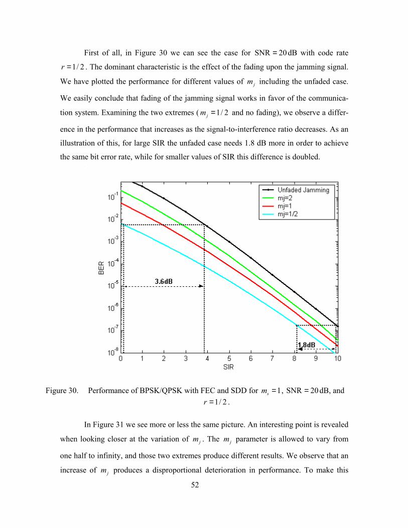
52
First of all, in Figure 30 we can see the case for SNR 20= dB with code rate
1/ 2r = . The dominant characteristic is the effect of the fading upon the jamming signal.
We have plotted the performance for different values of jm including the unfaded case.
We easily conclude that fading of the jamming signal works in favor of the communica-
tion system. Examining the two extremes ( 1/ 2jm = and no fading), we observe a differ-
ence in the performance that increases as the signal-to-interference ratio decreases. As an
illustration of this, for large SIR the unfaded case needs 1.8 dB more in order to achieve
the same bit error rate, while for smaller values of SIR this difference is doubled.
Figure 30. Performance of BPSK/QPSK with FEC and SDD for 1sm = , SNR 20= dB, and 1/ 2r = .
In Figure 31 we see more or less the same picture. An interesting point is revealed
when looking closer at the variation of jm . The jm parameter is allowed to vary from
one half to infinity, and those two extremes produce different results. We observe that an
increase of jm produces a disproportional deterioration in performance. To make this
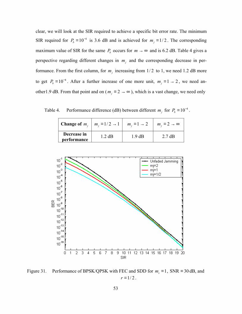
53
clear, we will look at the SIR required to achieve a specific bit error rate. The minimum
SIR required for 410bP −= is 3.6 dB and is achieved for 1/ 2jm = . The corresponding
maximum value of SIR for the same bP occurs for m → ∞ and is 6.2 dB. Table 4 gives a
perspective regarding different changes in jm and the corresponding decrease in per-
formance. From the first column, for jm increasing from 1/ 2 to 1, we need 1.2 dB more
to get 410bP −= . After a further increase of one more unit, 1 2jm = → , we need an-
other1.9 dB. From that point and on ( 2jm = → ∞ ), which is a vast change, we need only
Table 4. Performance difference (dB) between different jm for 410bP −= .
Change of jm 1/ 2 1jm = → 1 2jm = → 2jm = → ∞
Decrease in performance
1.2 dB 1.9 dB 2.7 dB
Figure 31. Performance of BPSK/QPSK with FEC and SDD for 1sm = , SNR 30= dB, and 1/ 2r = .
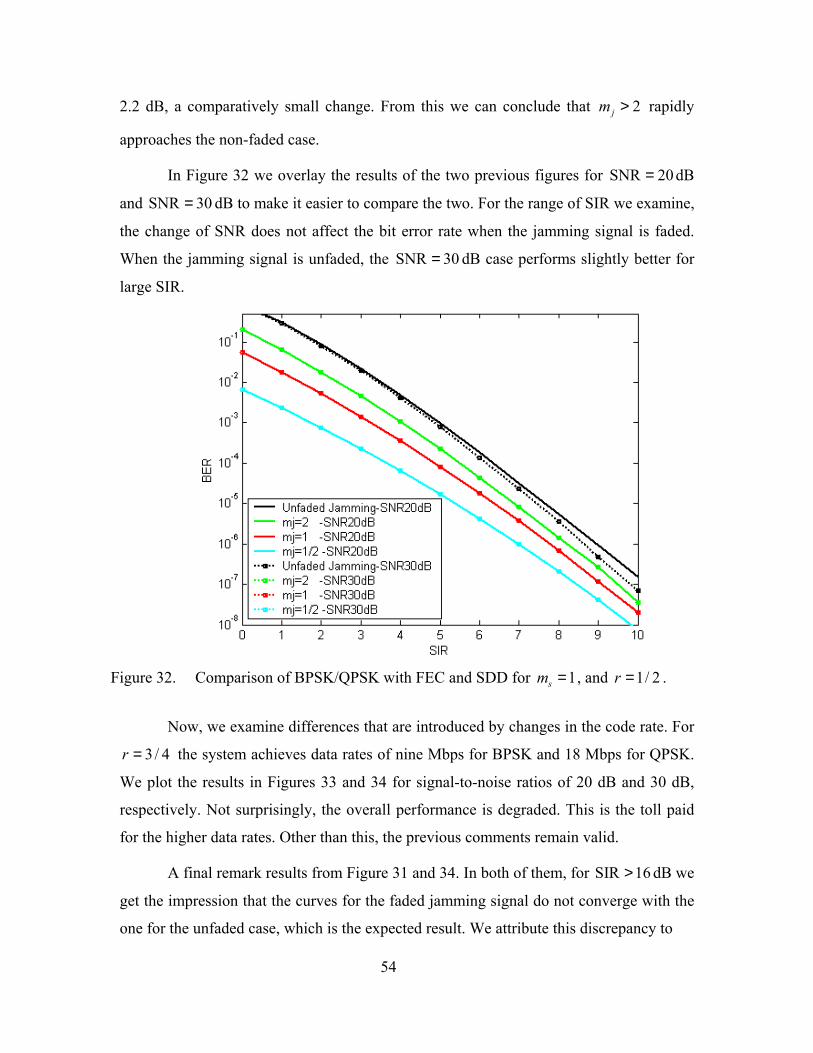
54
2.2 dB, a comparatively small change. From this we can conclude that 2jm > rapidly
approaches the non-faded case.
In Figure 32 we overlay the results of the two previous figures for SNR 20= dB
and SNR 30= dB to make it easier to compare the two. For the range of SIR we examine,
the change of SNR does not affect the bit error rate when the jamming signal is faded.
When the jamming signal is unfaded, the SNR 30= dB case performs slightly better for
large SIR.
Figure 32. Comparison of BPSK/QPSK with FEC and SDD for 1sm = , and 1/ 2r = .
Now, we examine differences that are introduced by changes in the code rate. For
3 / 4r = the system achieves data rates of nine Mbps for BPSK and 18 Mbps for QPSK.
We plot the results in Figures 33 and 34 for signal-to-noise ratios of 20 dB and 30 dB,
respectively. Not surprisingly, the overall performance is degraded. This is the toll paid
for the higher data rates. Other than this, the previous comments remain valid.
A final remark results from Figure 31 and 34. In both of them, for SIR 16> dB we
get the impression that the curves for the faded jamming signal do not converge with the
one for the unfaded case, which is the expected result. We attribute this discrepancy to
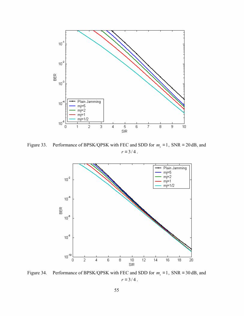
55
Figure 33. Performance of BPSK/QPSK with FEC and SDD for 1sm = , SNR 20= dB, and 3 / 4r = .
Figure 34. Performance of BPSK/QPSK with FEC and SDD for 1sm = , SNR 30= dB, and
3 / 4r = .
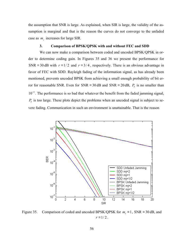
56
the assumption that SNR is large. As explained, when SIR is large, the validity of the as-
sumption is marginal and that is the reason the curves do not converge to the unfaded
case as jm increases for large SIR.
3. Comparison of BPSK/QPSK with and without FEC and SDD We can now make a comparison between coded and uncoded BPSK/QPSK in or-
der to determine coding gain. In Figures 35 and 36 we present the performance for
SNR 30= dB with 1/ 2r = and 3 / 4r = , respectively. There is an obvious advantage in
favor of FEC with SDD. Rayleigh fading of the information signal, as has already been
mentioned, prevents uncoded BPSK from achieving a small enough probability of bit er-
ror for reasonable SNR. Even for SNR 30= dB and SNR 20= dB, bP is no smaller than
310− . The performance is so bad that whatever the benefit from the faded jamming signal,
bP is too large. These plots depict the problems when an uncoded signal is subject to se-
vere fading. Communication in such an environment is unattainable. That is the reason
Figure 35. Comparison of coded and uncoded BPSK/QPSK for 1sm = , SNR 30= dB, and
1/ 2r = .
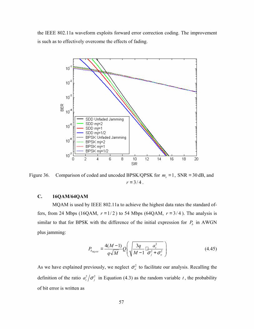
57
the IEEE 802.11a waveform exploits forward error correction coding. The improvement
is such as to effectively overcome the effects of fading.
Figure 36. Comparison of coded and uncoded BPSK/QPSK for 1sm = , SNR 30= dB, and
3 / 4r = .
C. 16QAM/64QAM MQAM is used by IEEE 802.11a to achieve the highest data rates the standard of-
fers, from 24 Mbps (16QAM, 1/ 2r = ) to 54 Mbps (64QAM, 3 / 4r = ). The analysis is
similar to that for BPSK with the difference of the initial expression for bP in AWGN
plus jamming:
2
2 2
4( 1) 31MQAM
cb
j o
aM qP QMq M σ σ
−= ⋅ − + (4.45)
As we have explained previously, we neglect 2oσ to facilitate our analysis. Recalling the
definition of the ratio 2 2c ja σ in Equation (4.3) as the random variable t , the probability
of bit error is written as
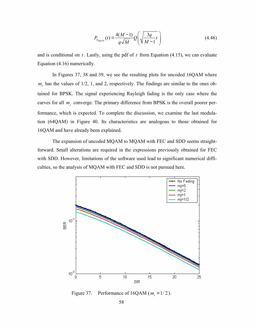
58
4( 1) 3( )1MQAMb
M qP t Q tMq M
−= − (4.46)
and is conditional on t . Lastly, using the pdf of t from Equation (4.15), we can evaluate
Equation (4.16) numerically.
In Figures 37, 38 and 39, we see the resulting plots for uncoded 16QAM where
sm has the values of 1/2, 1, and 2, respectively. The findings are similar to the ones ob-
tained for BPSK. The signal experiencing Rayleigh fading is the only case where the
curves for all jm converge. The primary difference from BPSK is the overall poorer per-
formance, which is expected. To complete the discussion, we examine the last modula-
tion (64QAM) in Figure 40. Its characteristics are analogous to those obtained for
16QAM and have already been explained.
The expansion of uncoded MQAM to MQAM with FEC and SDD seems straight-
forward. Small alterations are required in the expressions previously obtained for FEC
with SDD. However, limitations of the software used lead to significant numerical diffi-
culties, so the analysis of MQAM with FEC and SDD is not pursued here.
Figure 37. Performance of 16QAM ( 1/ 2sm = ).
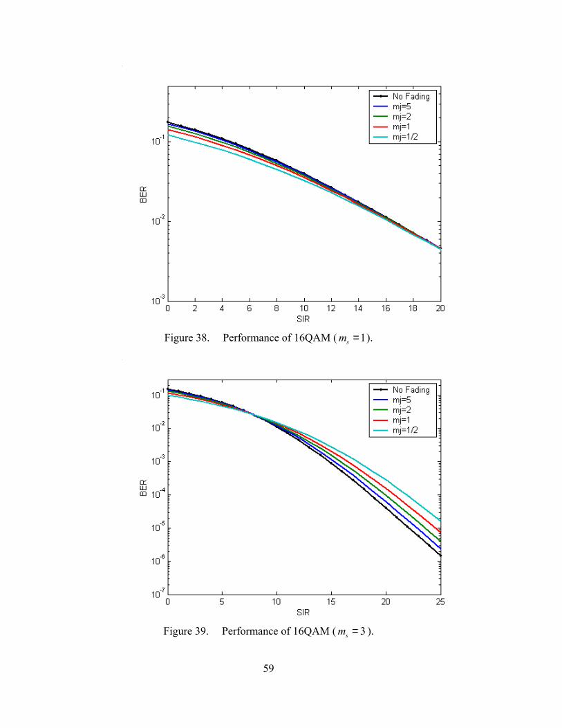
59
Figure 38. Performance of 16QAM ( 1sm = ).
Figure 39. Performance of 16QAM ( 3sm = ).
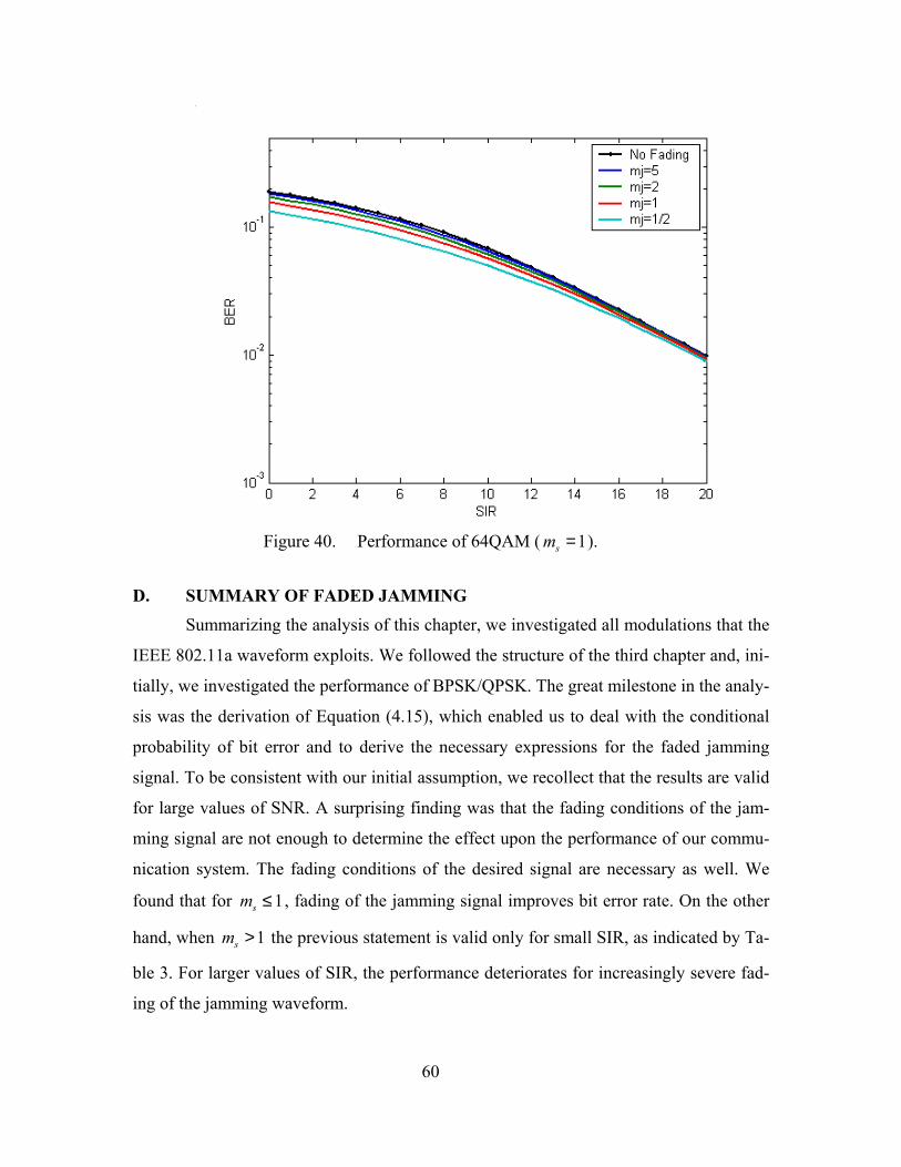
60
Figure 40. Performance of 64QAM ( 1sm = ).
D. SUMMARY OF FADED JAMMING
Summarizing the analysis of this chapter, we investigated all modulations that the
IEEE 802.11a waveform exploits. We followed the structure of the third chapter and, ini-
tially, we investigated the performance of BPSK/QPSK. The great milestone in the analy-
sis was the derivation of Equation (4.15), which enabled us to deal with the conditional
probability of bit error and to derive the necessary expressions for the faded jamming
signal. To be consistent with our initial assumption, we recollect that the results are valid
for large values of SNR. A surprising finding was that the fading conditions of the jam-
ming signal are not enough to determine the effect upon the performance of our commu-
nication system. The fading conditions of the desired signal are necessary as well. We
found that for 1sm ≤ , fading of the jamming signal improves bit error rate. On the other
hand, when 1sm > the previous statement is valid only for small SIR, as indicated by Ta-
ble 3. For larger values of SIR, the performance deteriorates for increasingly severe fad-
ing of the jamming waveform.
61
Continuing, we narrowed the possible signal fading conditions to Rayleigh due to
practical difficulties encountered in the numerical evaluation required for FEC with SDD.
Thus, we derived Equation (4.39), which is the core of the chapter concerning coded per-
formance. Although it is expressed in the Laplace domain, the use of the numerical in-
verse of the two-sided Laplace transformation from [9] easily overcame that difficulty.
The resulting plots reinforced the validity of the findings for uncoded BPSK for the
1jm = case. Moreover, it became apparent that FEC with SDD is essential when there is
severe signal fading, since FEC with SDD tremendously improves the bit error rate.

62
THIS PAGE INTENTIONALLY LEFT BLANK
63
V. CONCLUSION
A. INTRODUCTION The goal of this thesis was to investigate the performance of WLAN systems. Due
to its popularity and its high data rates, we selected IEEE 802.11a standard as a represen-
tative standard. Using the actual characteristics of the standard, we investigated all modu-
lation types the standard specifies. Additionally, we examined the informational signal
with and without FEC with SDD.
In every case we studied, the effect of fading and pulsed-noise jamming was con-
sidered. The study of FEC with SDD revealed significant results that support the use of
error correction to mitigate effects of fading. Then we incorporated into the analysis the
effect of the fading channel on the jamming signal to obtain a realistic estimate of the ef-
fect of hostile jamming when the information signal is transmitted over a fading channel.
B. FINDINGS
We began the analysis in Chapter III, where the fading channel was assumed to
affect only the informational signal. The result was that performance for a signal with
FEC and SDD and for a signal without coding exhibits the same characteristics; as sm
increases, performance improves. Examining the optimum strategy for pulsed-noise
jamming, we tested different values of p . We found that continuous jamming is most
effective when the receiver employs coding in all fading environments.
In Chapter IV we introduced fading of the jamming signal. Without FEC with
SDD, fading of the jamming signal decreased the probability of bit error for all modula-
tion types when 1sm ≤ . For larger values of sm and for small SIR, the probability of bit
error was again decreased as the fading of the jamming signal became more severe. The
opposite behavior was seen when SIR was increased, when performance deteriorated.
Based on the finding that the worst-case for signals with FEC and SDD is con-
tinuous jamming, we used 1p = for the analysis in the second part of Chapter IV, where
the signal employed FEC with SDD. The cases of fading of the desired signal we studied
64
were limited to Rayleigh due to extreme complexity of the calculations when 1sm ≠ . In
this case a decrease of jm improves performance.
C. RECOMMENDATIONS FOR FURTHER RESEARCH Although this thesis focuses on IEEE 802.11a signals, the findings can be used in
a broad field of communication systems. Every system utilizing either MPSK or MQAM
with FEC with SDD and pulsed-noise jamming can be examined using our analysis.
Small alterations regarding the code rate and the encoder are enough to find the perform-
ance of other standards. The same is true as regards the study of the effect of fading on
the jamming signal. Additionally, the approach followed can be exploited even when in-
vestigating MFSK modulation.
Our results are heavily based on numerical evaluations. If the analysis can be
taken further analytically, some of the numerical difficulties encountered here might be
avoided. The generation of plots for the cases we did not pursue might be feasible, like
the performance for modulations other than BPSK/QPSK when the jamming signal ex-
periences fading and the fading of the desired signal is other than Rayleigh.
The methodology of the numerical inverse of the two-sided Laplace transform
from [9] was a key point. Numerical evaluation would not be realizable without its use in
Chapters III and IV. It is the pillar of this work and will be useful to anyone facing prob-
lems of this nature. Nonetheless, additional research might focus on techniques to mini-
mize numerical problems that are sometimes encountered using this methodology.
Regarding OFDM, further research could investigate different options for the dis-
tribution of m . We arbitrary assumed m to be uniformly distributed, and we ranged its
value from one half to five. More accurate results would be produced by a study with
field measurements to determine the actual range of m .
D. CLOSING COMMENTS
WLANs are increasingly important in meeting the demand for high data rates.
FEC with SDD and OFDM offer the potential to mitigate fading effects and achieve sub-

65
stantial performance improvement. Their analysis is essential, since WLANs enjoy
acceptance from the broadband wireless communications systems of the next generation.

66
THIS PAGE INTENTIONALLY LEFT BLANK
67
LIST OF REFERENCES
1. L. Wan and V.K. Dubey, “Bit Error Probability of OFDM Systems Over Fre-quency-nonselective Fast Rayleigh Fading Channels,” IEE Electronics Letters, vol. 36, pp. 1306-07, July 2000.
2. L. Wan and V.K. Dubey , “BER Probability of OFDM Systems Over Frequency-nonselective Fast Ricean Fading Channels,” IEE Electronics Letters, vol. 5, pp. 19-21, January 2001.
3. Count A. Patrick, “Performance Analysis of OFDM Frequency-Selective, Slowly Fading Nakagami Channels,” Master’s Thesis, Naval Postgraduate School, Mon-terey, California, 2001.
4. Irfan Kosa, “Performance of IEEE 802.11a Wireless LAN Standard over Fre-quency-Selective, Slowly Fading Nakagami Channels in a Pulsed Jamming Envi-ronment,” Master’s Thesis, Naval Postgraduate School, Monterey, California, 2002.
5. John D. Oetting, “The Effects of Fading on Antijam Performance Requirements,” IEEE Journal on Selected Areas in Communications, vol. SAC-5, no. 2, pp. 155-161, February 1987.
6. A. H. Wojnar, ”Unknown Bounds on Performance in Nakagami Channels,” IEEE Trans. Commun., vol. COM-34, pp. 22-24, January 1986.
7. Bruce McGuffin, “Jammed FH-FSK Performance in Rayleigh and Nakagami-m Fading,” Proc. of MILCOM 2003.
8. Minoru Nakagami, “The m-Distribution – A General Formula of Intensity Distri-
bution of Rapid Fading,” in Statistical Methods in Radio Wave Propagation, W. C. Hoffman (ed.), pp. 3-36, Pergamon Press, New York, 1960.
9. Clark Robertson, Notes for EC4550 (Digital Communications), Naval Postgradu-ate School, Monterey, California, 2003 (unpublished).

68
10. Institute of Electrical and Electronics Engineers, 802.11a, Wireless LAN Medium Access Control (MAC) and Physical Layer (PHY) Specifications: High-Speed Physical Layer Extension in the 5 GHz Band, 16 September 1999.
11. B. Sklar, Digital Communications: Fundamental and Applications, 2nd ed., Pren-tice Hall, Upper Saddle River, New Jersey, 2002.
12. Clark Robertson, Notes for EC4580 (Coding and Information), Naval Postgradu-ate School, Monterey, California, 2001 (unpublished).
13. Theodore S. Rappaport, Wireless Communications Principles and Practice, 2nd ed., Prentice Hall, Upper Saddle River, New Jersey, 2002.
14. J.G. Proakis, Digital Communications, 4th ed., McGraw Hill, New York, 2001.
15. A. Papoulis, Probability, Random Variables, and Stochastic Processes, 3nd ed., McGraw Hill, New York, 1991.
16. I.S. Gradshteyn and I.M. Ryzhik, Tables of Integrals, Series, and Products, Aca-demic Press, New York, 1980.

69
INITIAL DISTRIBUTION LIST
1. Defense Technical Information Center Ft. Belvoir, Virginia
2. Dudley Knox Library Naval Postgraduate School Monterey, California
3. Chairman, Code EC/Po Department of Electrical and Computer Engineering Naval Postgraduate School Monterey, California
4. Chairman, Code SM/Bo Department of Information Science Naval Postgraduate School Monterey, California
5. Professor R. Clark Robertson EC/Rc Department of Electrical and Computer Engineering Naval Postgraduate School Monterey, California
6. Professor Donald van Zelm Wadsworth EC/Wd Department of Electrical and Computer Engineering & Space Systems Academic Group Naval Postgraduate School Monterey, California
7. Embassy of Greece Office of Naval Attache Washington, DC
8. 18 Anakreontos st.
Andreas Tsoumanis Egaleo-Athens, Greece 12243