Embed Size (px)
Citation preview
NAVAL POSTGRADUATE SCHOOLMonterey, California
AD-A261 820
•R AD10'%
DTICS ELECTE
MARI9 199311THESIS S E Dw
A COMPUTER ANALYSIS OF PROPORTIONAL NAVIGATIONAND COMMAND TO LINE OF SIGHT OF A COMMAND
GUIDED MISSILE FOR A POINT DEFENCE SYSTEM
by
Dimitrios loannis Peppas
December, 1992
Thesis Advisor: Harold A. Titus
Approved for public release; distribution is unlimited.
93--05787
UNCLASSIFIEDSEC U R I -V C .A SS ,F ,CA :O N 01 "' W A 77.G E
REPORT DOCUMENTATION PAGE orNo 070oo-0e1
la REPORT SECURITY C•ASSiFiCATION II RE SRiC-ývE MARK:NGS
UNCLASSIFIED2a SECURITY CLASSIFICATION AuTHORiTY 3 DISTRIBk_;0N AiA LAB:, T7 OI •P:OZ-
Approved for Public Release;20 DECLASS•FCA'ON ZOWNGRADING SCHEDULE distribution is unlimited.
4 PER=ORMING ORGANIZATION REPORT NUMBER(Sj 5 MONfTORiNG ORGANZAT ON REPO2 N-MBER:S.
6a NAME OF PERFORMING ORGANiZATiON 6o OFFICE SYMBOL 7a NAME O1 MON!TORiNG O0GAN -'A- 0%
(If applicable)
Naval Postgraduate School EC Naval Postgraduate School
6c ADDRESS ICity, State, and ZIPCode) 7
o ADDRESS iCiry State and ZIP Code)
Monterey, CA 93943 Monterey, CA 93940
Ba NAME OF FJNDING SPONSORING Bo OFFICE SYMBO- 9 PROCiREMEN- INSR.ZMEN- !DEN71F(CAQO% \%BEPORGANIZATION (If applicable)
8c ADDRESS (City, State, and ZIP Code) 10 SO.,RCE 03 K'NDING NUMBERS
PROGRAM OROjEC7 IASK -NAOR• UNiTELEMENT NO NO NO A.CCESSION NO
"11 TITLE (include Security Classification) A Computer Analysis of Proportional Navigation and Command toLine of Sight of a Command Guide ED Missile for A Point Defence System.
12 PERSONAL, AUTHOR(S)Dimtrios loannis Peppas
13a TYPE OF REPORT 3b TIME COVERED 14 DATE OF REPORT (Year, Month Day) 5 PACE C: I.
Master's THesis FROM_ TO I December 1992[ 13716 SUPDLEMENTARY NOTATION The views expressed in this thesis are those of the author and do
not reflect the official policy or position of the Department of Defense or the United
17 COSAT; CODES 18 SUBJECT TERMS (Continue on reverse if necessary and ,dentity oy bloc, number)
FIELD GROUP SUB-GROUP Proportional Navigation Command Guidance, Command to Lineof Sight Guidance, Missile Guidance, Missile Simulation
19 ABSTRACT (Continue on reverse if necessary and identify by block number)
This thesis compares two types of command guidance to be used by a point defense
system: Proportional Navigation and Command to Line Of Sight (CLOS). The systemblock diagram was first defined. The necessary transfer functions were derived.
Two forward time models were evaluated, one for each guidance method, using statevariable analysis. Two three dimensional scenarios were defined and their resultsused to compare the two methods. Parameters considered in the comparison were miss
distance and acceleration load on the missile.
10 DS'PIBU'1ON A4A-4,ýAI-Y W7 ABSTRACT 21 ABSTRACT SECuRITý CýASS :,CA7,ON
[ .JNiC-ASSI; ED,;r•IIE 0 SAME AS PO" [ DTC JSEPS UNCLASSIFIED
Zla 0.~' ;P-- OS=. %D V0,.if- 22b TE.EPHONE (include ,Area Code) •2Zc OF",C" S '%*30.
Titus, Harold A. 408-646-2560 1EC/Ts
DD Form 1473, JUN 86 Previous editions are obsolete S•C - CA•$ ;.- 0. D
S/N 0102-LF-014-6603 UNCLASSIFIED
i
Approved for public release; distribution is unlimited.
A Computer Analysis of Proportional Navigationand Command to Line of Sight of a Command
Guided Missile for a Point Defence System
by
Dimitrios I. PeppasLieutenant (junior grade), Hellenic Navy
B.S.E.E., Hellenic Naval Academy, 1984
Submitted in partial fulfillmentof the requirements for the degree of
MASTER OF SCIENCE IN ELECTRICAL ENGINEERING
from the
NAVAL POSTGRADUATE SCHOOL
Author: Dimitrios. Peppas
Approved by: 2
H dA.Tts, Thesi r
Roberto Cristi, Second Reader
Michael A. Morgan, ChairmanDepartment of Electrical and Computer Engineering
ABSTRACT
This thesis compares two types of command guidance to be used by a point defence system:
Proportional Navigation and Command to Line Of Sight (CLOS). The system block diagram was first
defined. The necessary transfer functions were derived. Two forward time models were evaluated,
one for each guidance method, using state variable analysis. Two three dimensional scenarios were
defined and their results used to compare the two methods. Parameters considered in the comparison
were miss distance and acceleration load on the missile.
Accesion For
NTIS CRA&IDTIC TABUnannouncedJustification
By .................................. ..... .........
Distribution I
Availability CodesAvail and b r
Dist Special
I
i
d
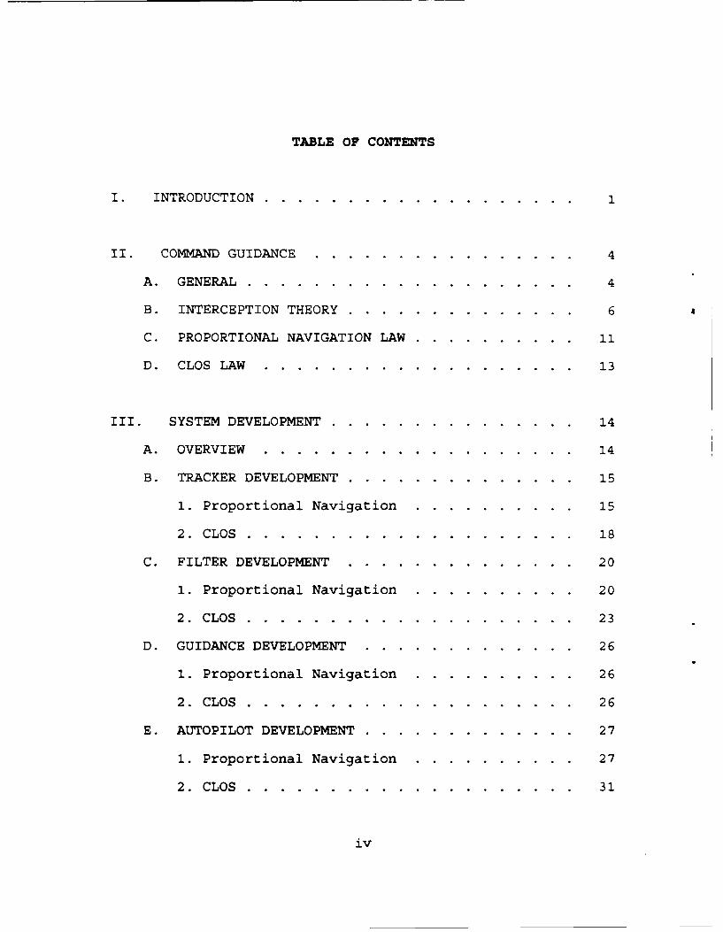
TABLE OF CONTENTS
I. INTRODUCTION ............ .................... .
II. COMMAND GUIDANCE ............... ................ 4
A. GENERAL ................... .................... 4
B. INTERCEPTION THEORY ............ .............. 6
C. PROPORTIONAL NAVIGATION LAW .... .......... 11
D. CLOS LAW ............. ................... 13
III. SYSTEM DEVELOPMENT ........ ............... 14
A. OVERVIEW ............... ................... 14
B. TRACKER DEVELOPMENT ........ .............. 15
1. Proportional Navigation ..... .......... 15
2. CLOS .............. .................... 18
C. FILTER DEVELOPMENT ......... .............. 20
1. Proportional Navigation ..... .......... 20
2. CLOS .............. .................... 23
D. GUIDANCE DEVELOPMENT ....... ............. 26
1. Proportional Navigation ..... .......... 26
2. CLOS .............. .................... 26
E. AUTOPILOT DEVELOPMENT ...... ............. 27
1. Proportional Navigation ..... .......... 27
2. CLOS .............. .................... 31
iv
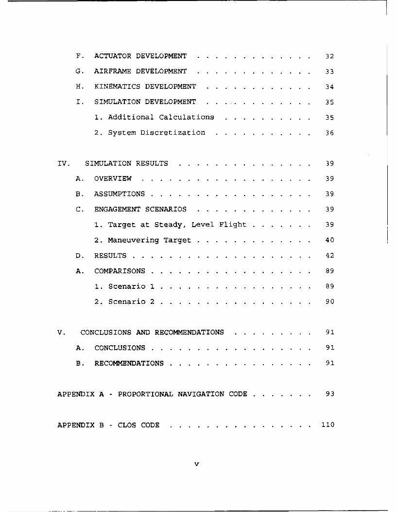
F. ACTUATOR DEVELOPMENT ......................... 32
G. AIRFRAME DEVELOPMENT ......................... 33
H. KINEMATICS DEVELOPMENT ....................... 34
I. SIMULATION DEVELOPMENT ....................... 35
1. Additional Calculations ................... 35
2. System Discretization ..................... 36
IV. SIMULATION RESULTS ........... ............... 39
A. OVERVIEW ............... ................... 39
B. ASSUMPTIONS ............ .................. 39
C. ENGAGEMENT SCENARIOS ....... ............. 39
1. Target at Steady, Level Flight.... . ...... 39
2. Maneuvering Target ...... ............. 40
D. RESULTS .............. .................... 42
A. COMPARISONS ............ .................. 89
1. Scenario 1 ............ ................. 89
2. Scenario 2 .......... ................. 90
V. CONCLUSIONS AND RECOMMENDATIONS ... ......... 91
A. CONCLUSIONS ............ .................. 91
B. RECOMMENDATIONS .......... ................ 91
APPENDIX A - PROPORTIONAL NAVIGATION CODE ......... .. 93
APPENDIX B - CLOS CODE ............... ................ 110
v
LIST OF REFERENCES ............. .................. 127
INITIAL DISTRIBUTION LIST ........ ............... 128
vi
ACKNOWLEDG.MEN'TS
I would like to thank God, for showing me the way, my father, who has alwaa• been there
for me, and my vwife Lena and my daughter Terry, for reminding me what it's all about.
I have had the privilege and the honor to have had Professor Hal Titus as my teacher and as
an advisor. His knowledge and devotion to his work is only surpassed by his dedication to his
students.
I would also like to thank the Hellenic Navy, who gave me the chance to fulfill a lifetime
dream.
Finally to the organization known as the Naval Postgraduate School, for giving me not only
an education, but most of all, a new way of thinking.
vii
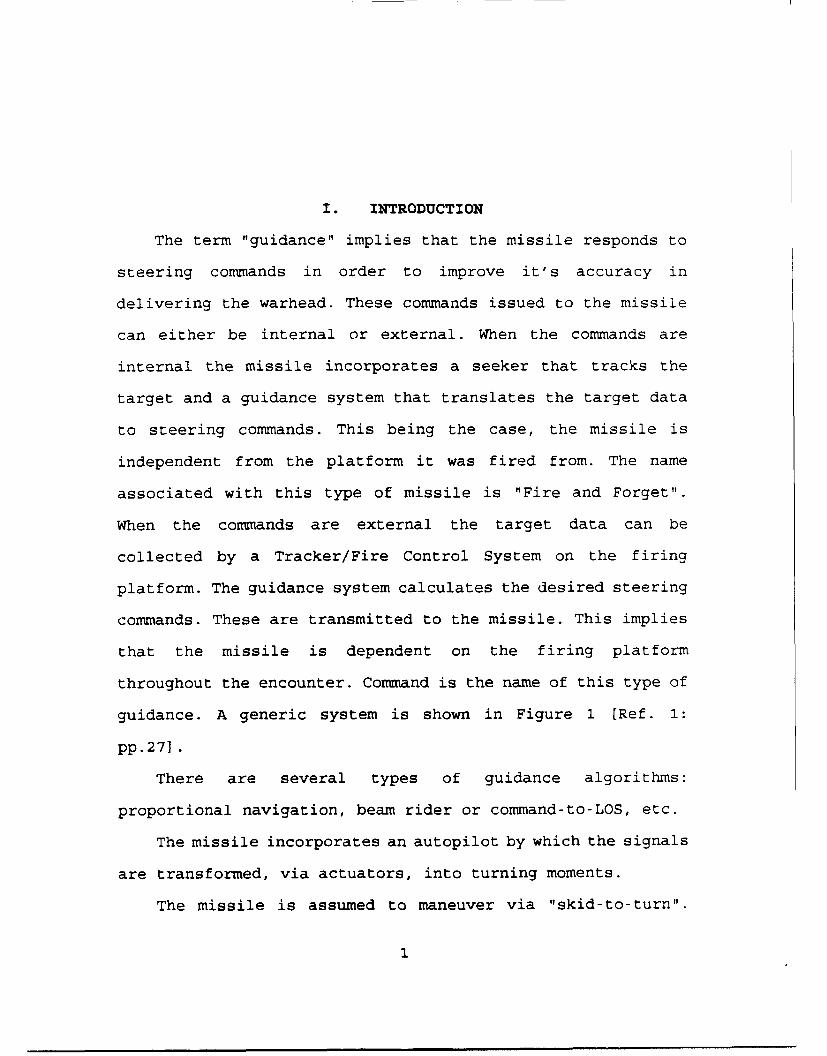
I. INTRODUCTION
The term "guidance" implies that the missile responds to
steering commands in order to improve it's accuracy in
delivering the warhead. These commands issued to the missile
can either be internal or external. When the commands are
internal the missile incorporates a seeker that tracks the
target and a guidance system that translates the target data
to steering commands. This being the case, the missile is
independent from the platform it was fired from. The name
associated with this type of missile is "Fire and Forget".
When the commands are external the target data can be
collected by a Tracker/Fire Control System on the firing
platform. The guidance system calculates the desired steering
commands. These are transmitted to the missile. This implies
that the missile is dependent on the firing platform
throughout the encounter. Command is the name of this type of
guidance. A generic system is shown in Figure 1 [Ref. 1:
pp.27].
There are several types of guidance algorithms:
proportional navigation, beam rider or command-to-LOS, etc.
The missile incorporates an autopilot by which the signals
are transformed, via actuators, into turning moments.
The missile is assumed to maneuver via "skid-to-turn".
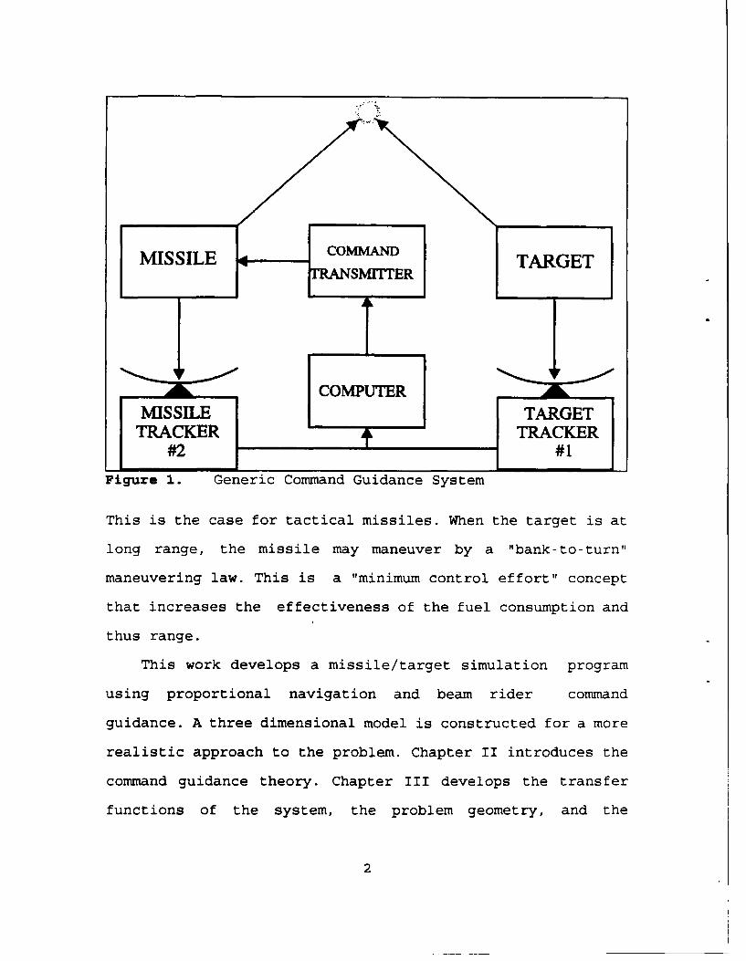
MISSILE COMMAND TARGETSMITTER
I ---
_ICOUTER_
MýSSILE TARGETTRACKER TRACKER
#2- #1
Figure 1. Generic Command Guidance System
This is the case for tactical missiles. When the target is at
long range, the missile may maneuver by a "bank-to-turn"
maneuvering law. This is a "minimum control effort" concept
that increases the effectiveness of the fuel consumption and
thus range.
This work develops a missile/target simulation program
using proportional navigation and beam rider command
guidance. A three dimensional model is constructed for a more
realistic approach to the problem. Chapter II introduces the
command guidance theory. Chapter III develops the transfer
functions of the system, the problem geometry, and the
2
relationships that are to be simulated. Chapter IV shows the
development of the computer code and relays the simulation
results. Chapter V discusses the conclusions and
recommendations.
This simulation uses MATLAB. The three dimensional plots
are generated from GRAFTOOL.
3
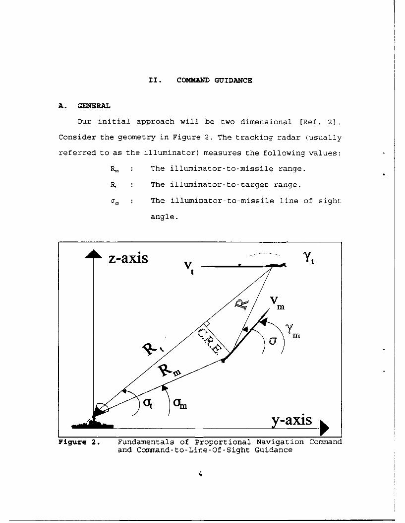
II. COMMAND GUIDANCE
A. GENERAL
Our initial approach will be two dimensional [Ref. 2]
Consider the geometry in Figure 2. The tracking radar (usually
referred to as the illuminator) measures the following values:
Rm: The illuminator-to-missile range.
, : The illuminator-to-target range.
0M : The illuminator-to-missile line of sight
angle.
z-a s y-axis
Figure 2. Fundamentals of Proportional Navigation Commandand Command- to- Line -Of -Sight Guidance
4
at, The illuminator-to-target line of sight
angle.
CRE The missile Cross Range Error from the
target tracking beam.
From these measurements, the Fire Control System solves for
the following values :
R The missile-to-target range.
R' : Rate of change of R.
a : The missile-to-target line of sight
angle.
a' Rate of change of a.
The guidance system of the Fire Control System now requires
that an interception can occur. This can happen by driving:
S= 0 (2.1)S< 0
or, by driving:
CRE = 0(2.2)
< 0
More insight on these relationships in the next section. But,
for now, the commands issued to the missile will affect the
following values:
vm The missile velocity.
'Yn : the missile flight path angle.
Finally, we know that the solution to the problem also depends
on:
5
V, The target velocity.
71 : The target flight path angle.
We will use here the Line of Sight (LOS) as that between
the target and the missile. This so as to reduce the quantity
of subscripts.
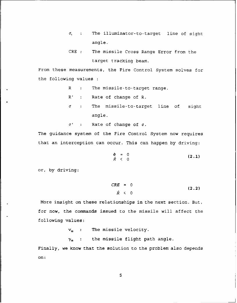
B. INTERCEPTION THEORY
The problem is to find a way by which the missile can hit
the target. Figure 3 shows several techniques developed to
solve this (Ref. 3: pp.3491. " Tail Chase", also known as
"Pure Pursuit", is the trajectory run through by a missile
aiming at the instantaneous position of the target. "Three
(a). Tail Chase (b). Constant Bearing
(c). Tbree Point
Figure 3. Interception Trajectories
6
Point" is the trajectory run through by the missile requiring
the three points: illuminator, missile and target to be on the
same line (LOS) at all times. These two techniques require a
highly maneuverable missile, able to withstand high
accelerations, induced by the large change of the missile
velocity vector, during the final seconds before impact (this
period is usually referred to as the "endgame").
Three point guidance is usually referred to as Command-to-
Line-Of-Sight (CLOS). This is based on the minimization of the
Cross Range Error (CRE);i.e. the displacement of the missile
from the illuminator-to-missile line of sight. The theory of
this technique is that since the three points are always on
the same line and the missile-to-target distance is always
shortening, these two are bound to meet. This explains the
relationships of Equations 2.2 of the previous section.
The simplest technique of all is the "Constant Bearing",
also known as "Optimum Pursuit". The theory behind this
technique is simple; if the missile "sees" the target at a
constant bearing (V'=0) and if the distance between the two is
continuously closing (R'<0), then the missile and target are
bound to collide. This explains the relationships of Equations
2.1 of the previous section. We define the closing velocity as
the negative rate of the LOS range:
v, = -R ý(2.3)
7
The benefits of this technique lie in the smaller acceleration
requirements during the endgame phase. Less missile energy is
also required [Ref. 4: pp. 26]. The guidance law associated
with this technique is called proportional navigation.
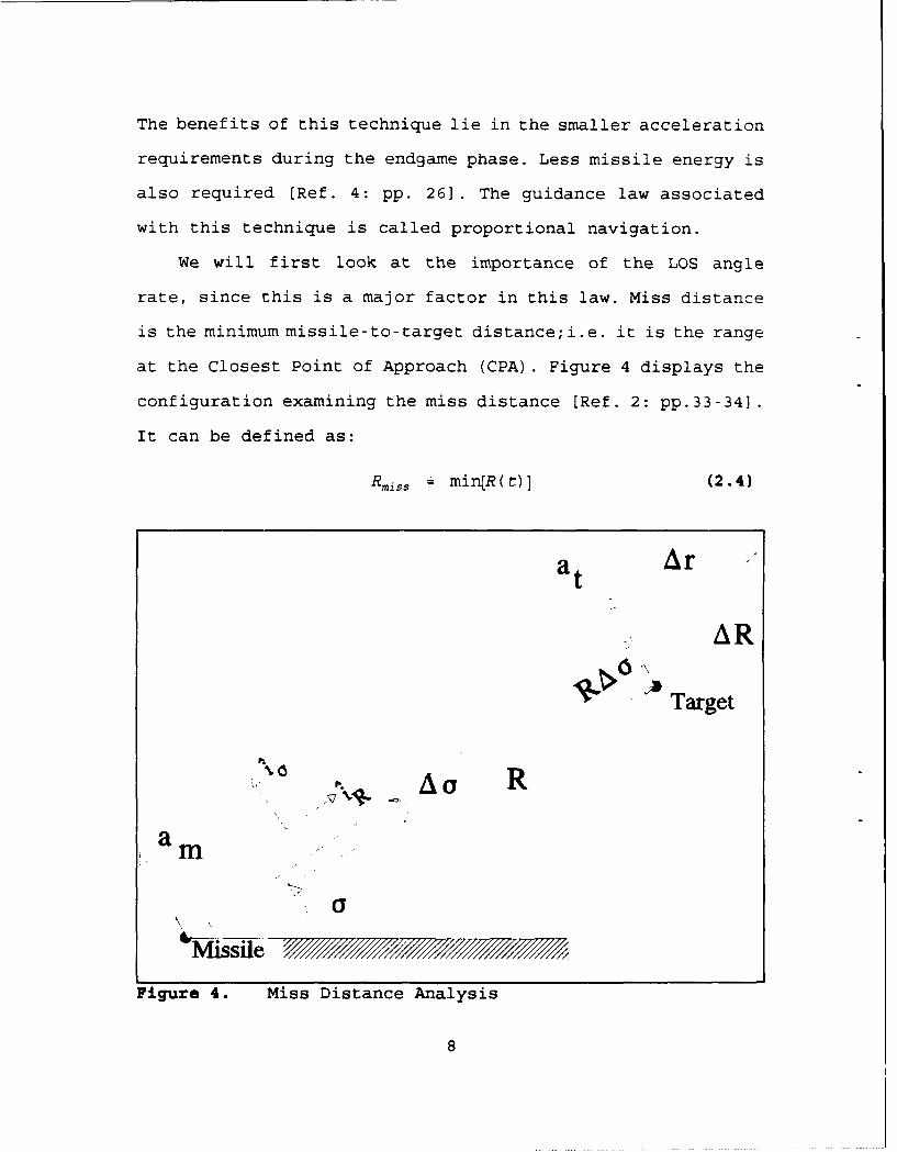
We will first look at the importance of the LOS angle
rate, since this is a major factor in this law. Miss distance
is the minimum missile-to-target distance;i.e. it is the range
at the Closest Point of Approach (CPA). Figure 4 displays the
configuration examining the miss distance [Ref. 2: pp.33-34].
It can be defined as:
Rmiss= mianR() ] (2.4)
at Ar
AR
Target
am
-Missile •'
Figure 4. Miss Distance Analysis
8
From vector theory, a vector quantity a , rotating with an
angular rate (&=do/dt) , is differentiated by the following
law:
- ÷ ,xA (2.5)dt t•
We must note here that aA/at is a vector parallel to
A and that A xB is perpendicular. This leads to the
incorporation of the orthogonal components i, and it,, as can
be seen in Figure 4. Also from the same Figure 4, we can see
that, an incremental increase in the LOS angle (Au), modifies
the LOS range rate:
AAt z + ARe A a(2.6)
At At
Taking the limit, of the above, as t-0, we have the derivative
of the LOS range. Following the law of Equation 2.5 we get:
S= I + XE (2.7)
Finding the acceleration of this rate again requires the use
of Equation 2.5, thus:
9
dA adt t+ (2.8)
j= f+A±Ax+xx
This acceleration is the vectorial difference of the missile
and target accelerations;i.e.:
tazget -•nissiie = •(2.9)
Componentwise, in the cross-range direction (parallel to 19):
t 0 ~= (~+2A)i 0 (2.10)
and in the range direction (parallel to 'R):
a R-m = (R-R62)IR (2.11)
In order to have a successful intercept, the cross range rate
of the LOS must be zero, thus from Equation 2.7, the
quantity .xR must be zero, implying either the LOS range
or the LOS angle rate must be zero. The case of them being
parallel is not physically attainable. Since the range is
generally not equal to zero, we are left with the zero LOS
angle rate. This implies that the LOS angle is constant and
also proves the first part of Equation 2.1. Furthermore,
Equations 2.10-11 show that constant LOS angle implies equal
missile and target normal acceleration components. Radial
acceleration components difference gives the closing
10

acceleration. We are now ready to develop the proportional
navigation law.
C. PROPORTIONAL NAVIGATION LAW
The acceleration command (a,) issued to the missile, by
the proportional navigation law, is perpendicular to the LOS.
The actual missile acceleration (am) is perpendicular to the
missile's velocity (vy) . Figure 5 depicts these relationships
[Ref. 11: pp. 8-11]. We now seek a connection between the
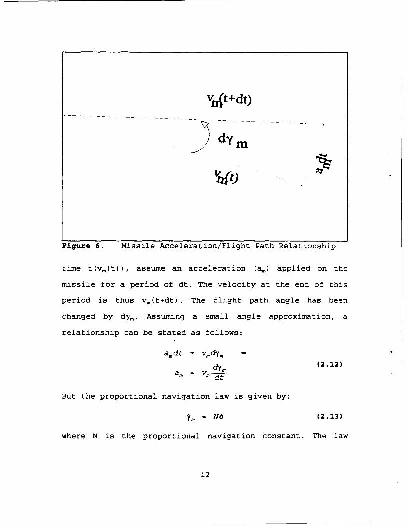
missile's acceleration and its flight path angle. Figure 6
depicts this relationship. Given the missile velocity at a
Vt TARGE
am V
Figure 5. Missile Accelerations
11
VrAt+dt)
dy m
WO
Figure 6. Missile Acceleration/Flight Path Relationship
time t(Vm(t)), assume an acceleration (a.) applied on the
missile for a period of dt. The velocity at the end of this
period is thus v,(t+dt) . The flight path angle has been
changed by dT.. Assuming a small angle approximation, a
relationship can be stated as follows:
amdt = vmdym 0
adym (2.12)a M = V. -j -t
But the proportional navigation law is given by:
fm = N6 (2.13)
where N is the proportional navigation constant. The law
12
states that the rate of change of the missile's flight path
angle is proportional to the rate of change of the LOS angle.
Substituting Equation 2.12 into Equation 2.13 yields:
am = vm N& (2.14)
The relationship connects the missile acceleration to the LOS
angular rate. The navigation constant usually ranges between
2 and 6.
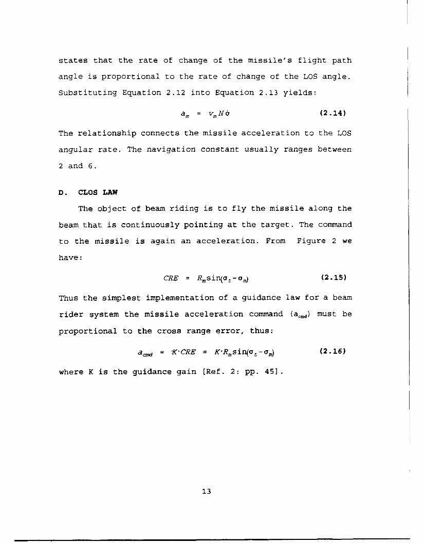
D. CLOS LAW
The object of beam riding is to fly the missile along the
beam that is continuously pointing at the target. The command
to the missile is again an acceleration. From Figure 2 we
have:
CRE = Rmsi~(ta-am) (2.15)
Thus the simplest implementation of a guidance law for a beam
rider system the missile acceleration command (acmd) must be
proportional to the cross range error, thus:
acm = K'CRE = K'Rmsin(t-am) (2.16)
where K is the guidance gain [Ref. 2: pp. 45].
13
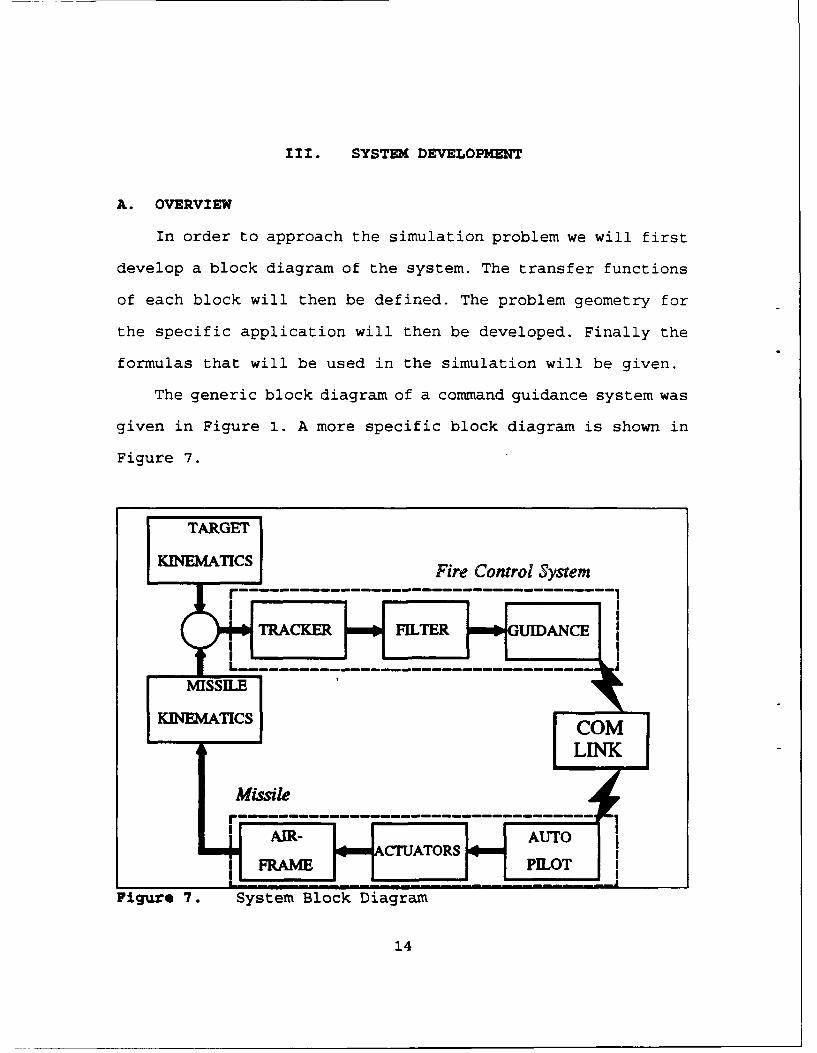
Ill. SYSTEM DEVELOPMENT
A. OVERVIEW
In order to approach the simulation problem we will first
develop a block diagram of the system. The transfer functions
of each block will then be defined. The problem geometry for
the specific application will then be developed. Finally the
formulas that will be used in the simulation will be given.
The generic block diagram of a command guidance system was
given in Figure 1. A more specific block diagram is shown in
Figure 7.
TARGET
KINEMATICS Fire Control SystemI 1
jTAKE+FILTER GIAC
L --------------MISSIIE
:AK• TMXCS [COM
-'"-7,LENK
Missile
r ---------------------------------- 1I AMR- AUT
Figure 7. System Block Diagram
14
B. TRACKER DEVELOPMENT
A tracker receives the radar return from the target, and
produces the illuminator-to-target range, and yaw and pitch
angles.
The yaw plane is defined as the xy-plane. The pitch plane
is the vertical plane containing the target and the missile.
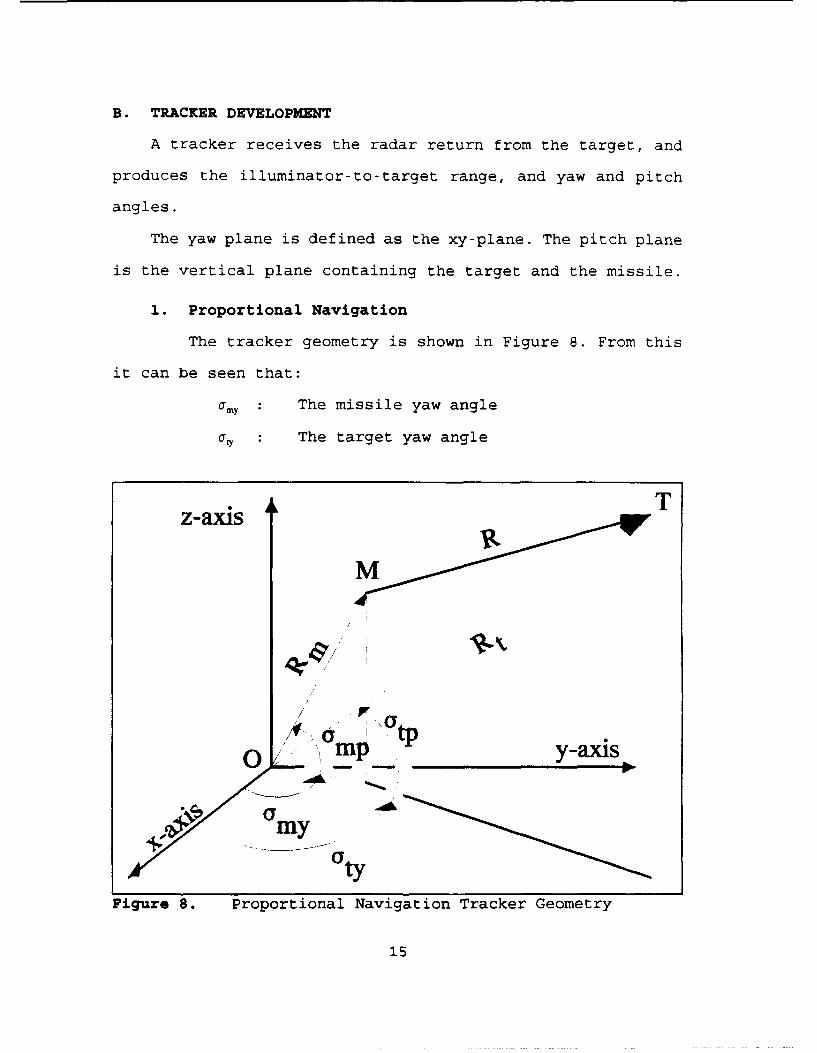
1. Proportional Navigation
The tracker geometry is shown in Figure 8. From this
it can be seen that:
amy : The missile yaw angle
arty The target yaw angle
z-axis T
mP y-axis
0tyFigure 8. Proportional Navigation Tracker Geometry
15
amp The missile pitch angle
( 4) The target pitch angle
Rm The illuminator-to-missile range
, : The illuminator-to-target range
R The missile-to-target range, also known as
the Miss Distance
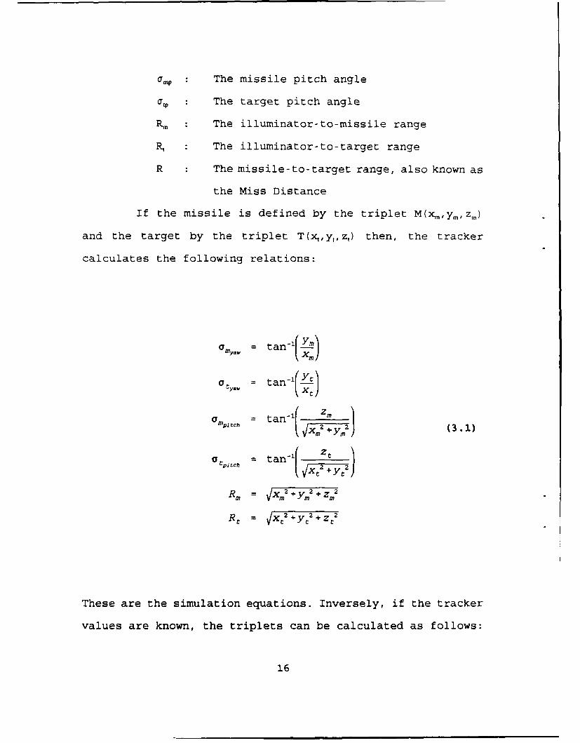
If the missile is defined by the triplet M(xVn,yt 1,zt.)
and the target by the triplet T(x,,y,,z,) then, the tracker
calculates the following relations:
a = tan-1 Y,]
amyam, = tan-(x' )
a = tan-1( zm (
tpi tch ran( X __Y2
~~ •h[ X"2 + y,2 (3.1i)a %i: = tan-1{ zxt+y2
Rm = •x 2 +YC 2 +z2
R t = Xt2 ÷yt2 ÷Zt2
These are the simulation equations. Inversely, if the tracker
values are known, the triplets can be calculated as follows:
16
Ym = (Rmcosasin)COSOmY.
YM= (Rmcos p tch )Sinalm
z , = Rsina -71P (3 .2)
= (Rc~s~.)c~o~(3.2)
xt (R,,os, ,,)co
zC = R~sinoa,,,:,
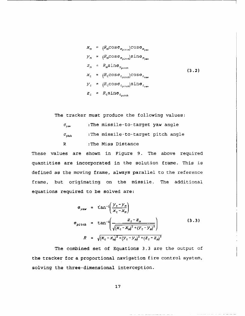
The tracker must produce the following values:
01yaw :The missile-to-target yaw angle
apitch :The missile-to-target pitch angle
R :The Miss Distance
These values are shown in Figure 9. The above required
quantities are incorporated in the solution frame. This is
defined as the moving frame, always parallel to the reference
frame, but originating on the missile. The additional
equations required to be solved are:
Oyaw = tan-1(YtY)x
apitch tan (' z( t -) zim (3.3)PI tchxt -x.)2 + (yC -y.) 2
R = V(Xt-Xm) 2 +(y,-ym)2 +(Zt-Zm) 2
The combined set of Equations 3.3 are the output of
the tracker for a proportional navigation fire control system,
solving the three-dimensional interception.
17
z Solution Frame
M ----------MM
a yymy . -
Ity
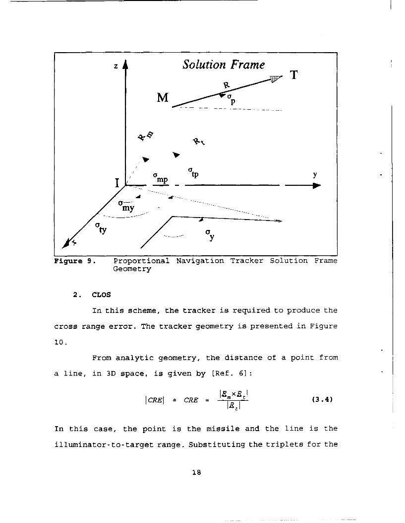
Figure 9. Proportional Navigation Tracker Solution FrameGeometry
2. CLOS
In this scheme, the tracker is required to produce the
cross range error. The tracker geometry is presented in Figure
10.
From analytic geometry, the distance of a point from
a line, in 3D space, is given by (Ref. 61:
ICREI - CRE = I~mוt (3.4)
In this case, the point is the missile and the line is the
illuminator-to-target range. Substituting the triplets for the
18

z T
M
CPPPM
ty/ .... 0tyY
Figure 10. CLOS Tracker Geometry
missile, M(xm,y, zm) , and the target, T(xyt, z,), the following
closed form solution for the cross range error, is derived:
CRE = - V(Xmyt:XCym)2 , (ymZtyyZm)2 , (ZmXCtZtXm) 2 (3.5)
The CRE components in the yaw and pitch plane can also
be calculated. Referring to Figure 10:
cRE, 8 w = Jxf ÷ 7 sini,,o.- ooyS = Xm 2 S yaw m ) (3 .6)
CREji = VCRE 2 - CRE,aw signPo - Urn)p itc h -i•,rh
The signum function is introduced in order to have a sign for
the pitch cross range error. This sign is transferred to the
commanded acceleration.
19
The combined set of Equations 3.5 and 3.6 are the
output of the tracker for a command-to-line-of-sight fire
control system, solving the three-dimensional interception.
C. FILTER DEVELOPMENT
1. Proportional Navigation
Proportional navigation guidance requires the rate of
change of the LOS angle. The filter estimates this rate from
the LOS angle observed by the missile.
The torque that will be applied to the missile will be
analogous to this estimated angular acceleration of the LOS
angle. The equation of motion describing the above is:
T = I1- (3.7)
where:
T : Control Torque
I : Moment of Inertia
S: Estimated LOS angular acceleration
The input value to the filter is the LOS angle. The output
value of the filter is its estimation of the angular
acceleration. In between it calculates the angular velocity of
the LOS. Thus solving for Equation 3.7 we get:
20

-T = -k 1 ([3-a)-k 2 (I (3.8)
= -k 2 O-k 1,+kla
where k1,k 2 are constants determined by the time constant used
by the tracker. Laplace transformation transfers Equation 3.8
from the time domain to the s-domain. Thus Equation 3.8
transformed evaluates the filter transfer function:
(S) (3.9)G(s) (s 2 +k2s+kl)
Assume the relationship:
1 1
For the system a time constant of 0.1 second was selected,
since it approximates current technology. So the constants can
be defined:
kI= ( 2= 100(3.11)
k2 = 20
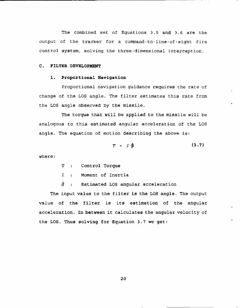
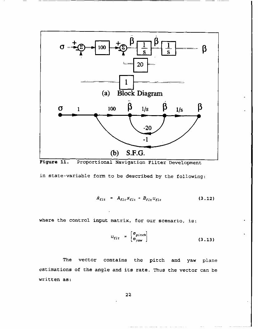
The block diagram and S.F.G. of the filter is shown in Figure
11.
From Figure 11 it can be seen that two integrators are
incorporated in the design. We can further analyze the system
21
G1
(a) Block Diagram
0 1100 P /s i /s P
-20
(b) S.F.G.Figure 11. Proportional Navigation Filter Development
in state-variable form to be described by the following:
kflt= Aflrxflt+ BfItfl= (3.12)
where the control input matrix, for our scenario, is:
Opi tchlUflt - . yaw J (3.13)
The vector contains the pitch and yaw plane
estimations of the angle and its rate. Thus the vector can be
written as:
22
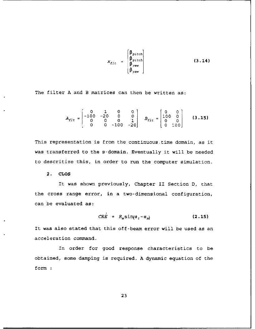
_ Opi tchlXf - piyrch (3.14)
- IPyaw
[i0yaw
The filter A and B matrices can then be written as:
0 1 0 01 0 0-10 0 0 I 100 0 (
fit 0 0 0 1 B = 0 0 (3.15)0 0 -100 -20] 0 1001
This representation is from the continuous-time domain, as it
was transferred to the s-domain. Eventually it will be needed
to descritize this, in order to run the computer simulation.
2. CLOS
It was shown previously, Chapter II Section D, that
the cross range error, in a two-dimensional configuration,
can be evaluated as:
CRE = Rmsi~l-G..m) (2.15)
It was also stated that this off-beam error will be used as an
acceleration command.
In order for good response characteristics to be
obtained, some damping is required. A dynamic equation of the
form
23
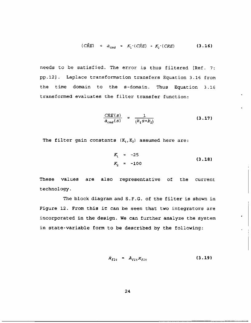
(CRE) - acnd = K1 '(CRE) - K2.(CRE) (3.16)
needs to be satisfied. The error is thus filtered [Ref. 7:
pp.12]. Laplace transformation transfers Equation 3.16 from
the time domain to the s-domain. Thus Equation 3.16
transformed evaluates the filter transfer function:
CRE(s) 1 (3.17)acmd (s) (kls+k2)
The filter gain constants (KIK 2) assumed here are:
K1 = -25(3.18)
K2= -100
These values are also representative of the current
technology.
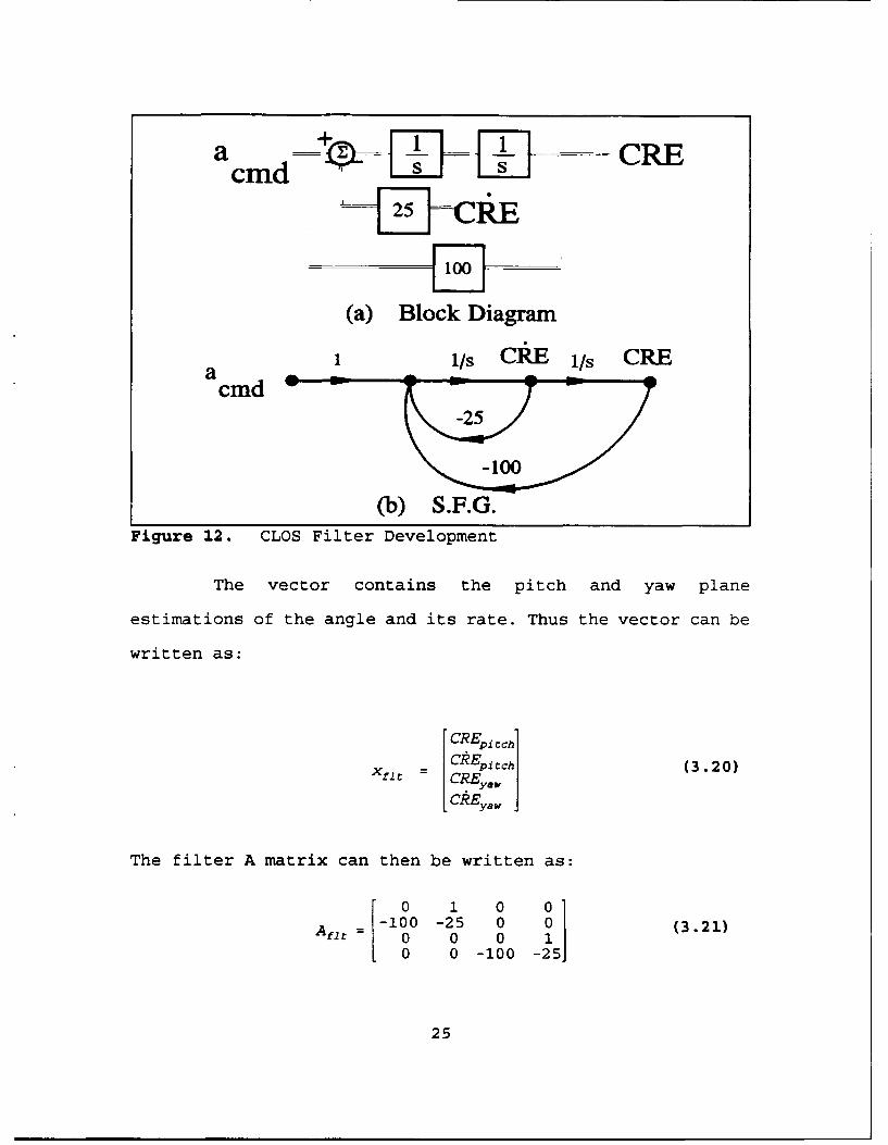
The block diagram and S.F.G. of the filter is shown in
Figure 12. From this it can be seen that two integrators are
incorporated in the design. We can further analyze the system
in state-variable form to be described by the following:
,kfit = Afltxflt (3.19)
24
a md + ' CREScmd L ~
25L fCRE
(a) Block Diagram
1 1/s ClE 1/s CRE
cmd-25
-100
(b) S.F.G.Figure 12. CLOS Filter Development
The vector contains the pitch and yaw plane
estimations of the angle and its rate. Thus the vector can be
written as:
CREPI Ch
CREpijtch (3.20)XI = CREy (32O
x f l tC R E Y , ,Ckyaw
The filter A matrix can then be written as:
0 1 0 0=-I00 -25 0 0 (3.21)
Al0 = 0 0 10 0 -100 -25]
25
This representation is from the continuous time domain, as it
was transferred to the s-domain. Eventually it will be needed
to descritize this, in order to run the computer simulation.
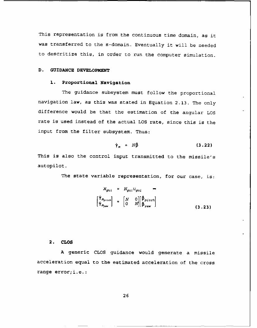
D. GUIDANCE DEVELOPMENT
1. Proportional Navigation
The guidance subsystem must follow the proportional
navigation law, as this was stated in Equation 2.13. The only
difference would be that the estimation of the angular LOS
rate is used instead of the actual LOS rate, since this is the
input from the filter subsystem. Thus:
=m = No (3.22)
This is also the control input transmitted to the missile's
autopilot.
The state variable representation, for our case, is:
X[Y i. = SN 02 [g i UW
IYW yi' 4fyaw '(3.23)
2. CLOS
A generic CLOS guidance would generate a missile
acceleration equal to the estimated acceleration of the cross
range error;i.e.:
26
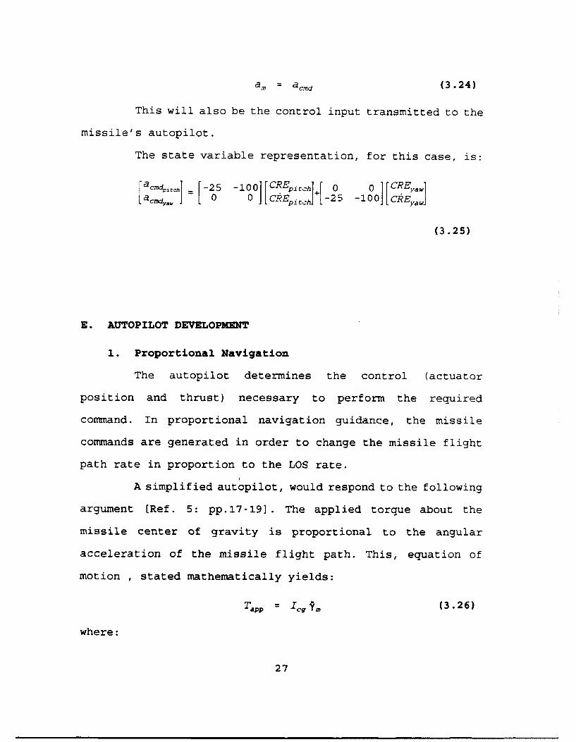
am = a Cad (3.24)
This will also be the control input transmitted to the
missile's autopilot.
The state variable representation, for this case, is:
a -d,,ld = 1-25 -100 CRE i c [ 0 1 0 CREY8WIacmd ] 0 JLCEpjj~ -25 100 CREY.W
(3.25)
E. AUTOPILOT DEVELOPMENT
1. Proportional Navigation
The autopilot determines the control (actuator
position and thrust) necessary to perform the required
command. In proportional navigation guidance, the missile
commands are generated in order to change the missile flight
path rate in proportion to the LOS rate.
A simplified autopilot, would respond to the following
argument [Ref. 5: pp.17-19]. The applied torque about the
missile center of gravity is proportional to the angular
acceleration of the missile flight path. This, equation of
motion , stated mathematically yields:
Tapp = Icg m (3.26)
where:
27
TPP : The applied torque
I•' The moment of inertia around the
missile's center of gravity
Ym : The angular acceleration of the
missile's flight path
The control torque, discussed in Chapter III Section
C, may be different from the applied torque. Thus solving
Equation 3.26 for the flight path acceleration:
?m Tapp -kgm+kNO (3.27)Icg
where k is determined by the slowest time constant of the
missile/autopilot. Laplace transformation transfers Equation
3.27 from the time domain to the s-domain. Thus Equation 3.27
transformed evaluates the autopilot transfer function:
Ym(s) - kNg-3(s) k (3.28)A(s) s +k
For the autopilot a time constant of 1.0 second was selected.
So the constant can be defined:
k = 1 = 1 (3.29)T ap
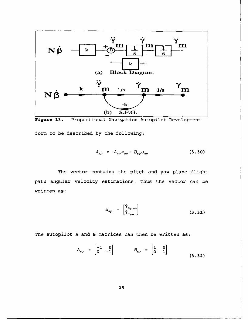
The autopilot block diagram and S.F.G. are shown in
Figure 13. From this it can be seen that although two
integrators are incorporated in the design, only one output is
fedback. We can further analyze the system in state-variable
28
N•
(a) Block Diagram
k fMl 1/s m 1/s Im
N *ýý -k
(b) S.F.G.
Figure 13. Proportional Navigation Autopilot Development
form to be described by the following:
.kap = AapXap + Bapuap (3.30)
The vector contains the pitch and yaw plane flight
path angular velocity estimations. Thus the vector can be
written as:
Xap L I (3.31)
The autopilot A and B matrices can then be written as:
Aap = [-l -01] Ba [1 (332[0 01 a0 1 (3.32)
29
The control input matrix is:
Uap = Bg~ Uguj1 [= 0 fpiCch]ýN O aw 1(3.33)
This representation is from the continuous time
domain, as it was transferred to the s-domain. Eventually it
will be needed to descritize this, in order to run the
computer simulation.
This direction change rate is converted to an
acceleration command to the actuators. First, the missile
velocity must be analyzed in the pitch and yaw plane.
Referring to Figure 14, the missile velocity vector components
can be stated as follows:
vmpit = Ivm cos(ym(., - (3.34)
S= I vmCOSYmpI
Then the acceleration components can be derived:
am =p VmPI 12 I Y p c h (3 .3 5 )
a..= v~ MYd, M.
The spatial accelerations are the same for the CLOS
autopilot and are derived in the following Subsection 2.
30
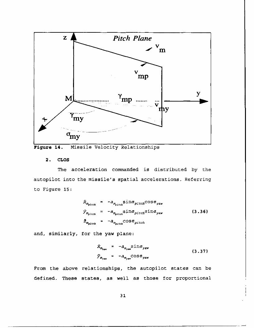
zz Pitch Plane
Vmp
M ........... Y p YM .............. M P_ . . . ... . ... .. .
Figure 14. Missile Velocity Relationships
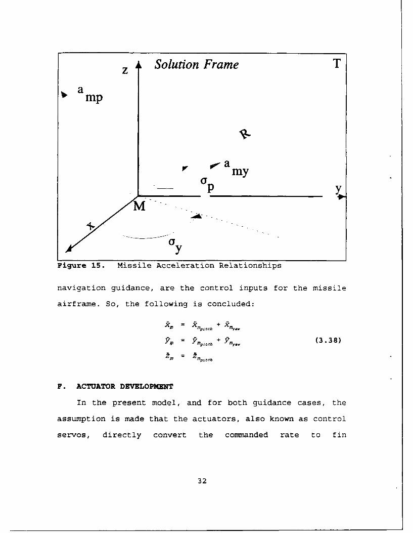
2. CLOS
The acceleration commanded is distributed by the
autopilot into the missile's spatial accelerations. Referring
to Figure 15:
J~p~h= -amp csinGpitchCOSOyw
5Ymv• = -a pt~sino.i tch5 1in yaw (3.3 6)
mpc = -am ~cCOSOpi
and, similarly, for the yaw plane:
Xmy - -am• sina~yw
-m. = amya.COSG yaw
From the above relationships, the autopilot states can be
defined. These states, as well as those for proportional
31
Solution Frame Taz
mp
a ,-ym
YY
Figure 15. Missile Acceleration Relationships
navigation guidance, are the control inputs for the missile
airframe. So, the following is concluded:
= S-m.,ch + in. (3.38)
F. ACTUATOR DEVELOPMENT
In the present model, and for both guidance cases, the
assumption is made that the actuators, also known as control
servos, directly convert the commanded rate to fin
32
deflections. This being the case, the transfer function is
unity.
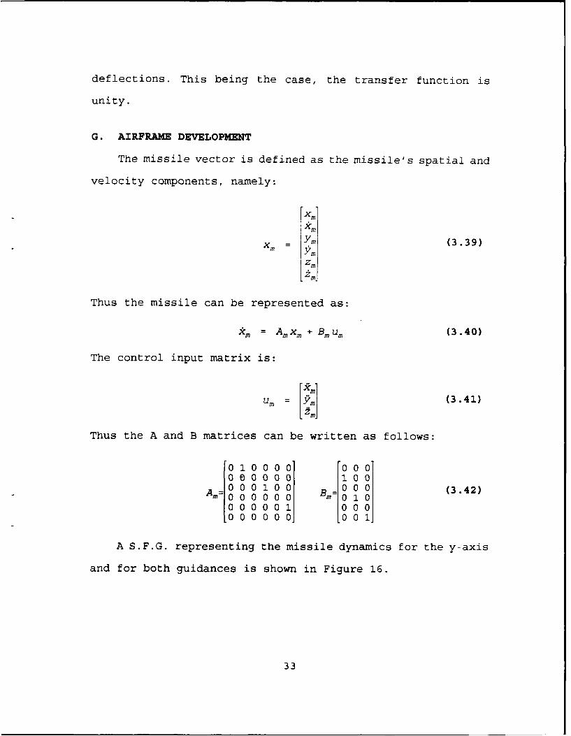
G. AIRFRAME DEVELOPMENT
The missile vector is defined as the missile's spatial and
velocity components, namely:
Ym (3.39)
ZM±.
Thus the missile can be represented as:
kfl Am.X• +BmUm (3.40)
The control input matrix is:
Urn (3.41)
Thus the A and B matrices can be written as follows:010000i 000i0 0 0 0 0 (3.42)Am0 0 0 0 0 B0 n 1 0
0 000 000 m0 10000001 0000 00 0 0O 00 1
A S.F.G. representing the missile dynamics for the y-axis
and for both guidances is shown in Figure 16.
33
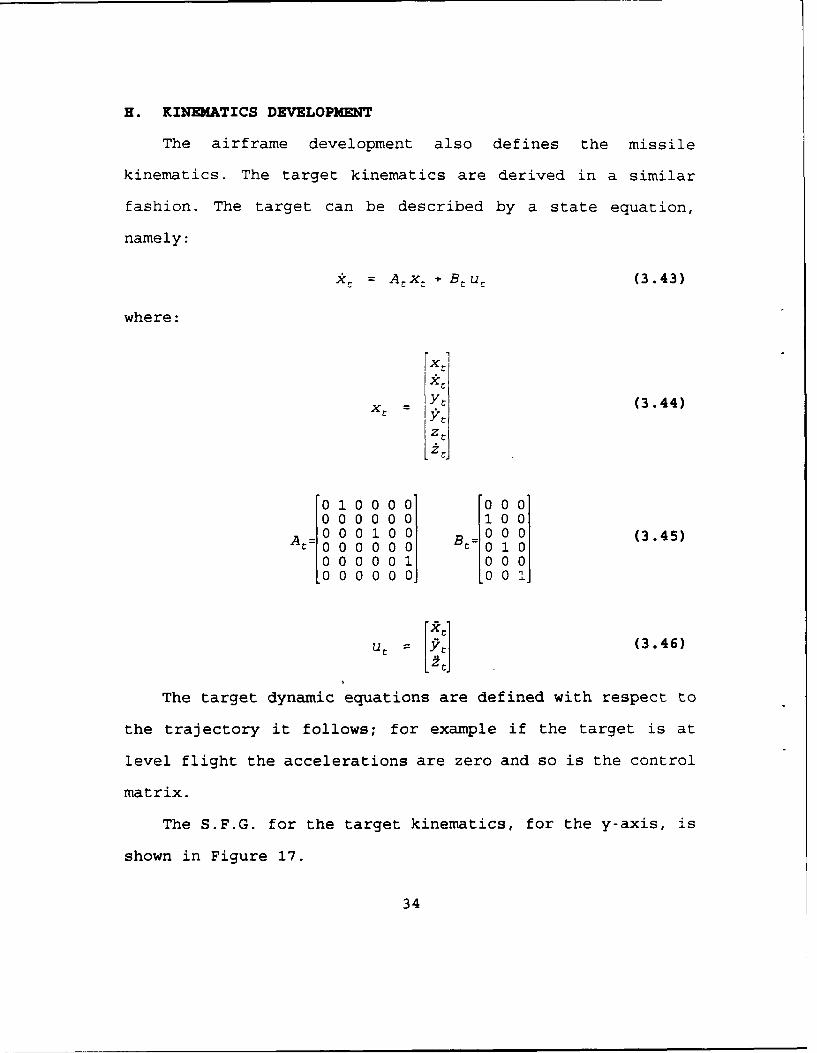
H. KINEMATICS DEVELOPMENT
The airframe development also defines the missile
kinematics. The target kinematics are derived in a similar
fashion. The target can be described by a state equation,
namely:
xk = ACx, + BCu (3.43)
where:
Xt
B•- (3.44)
S000000 t0
000001 000
000000 00
U [ = ý] (3.46)
The target dynamic equations are defined with respect to
the trajectory it follows; for example if the target is at
level flight the accelerations are zero and so is the control
matrix.
The S.F.G. for the target kinematics, for the y-axis, is
shown in Figure 17.
34
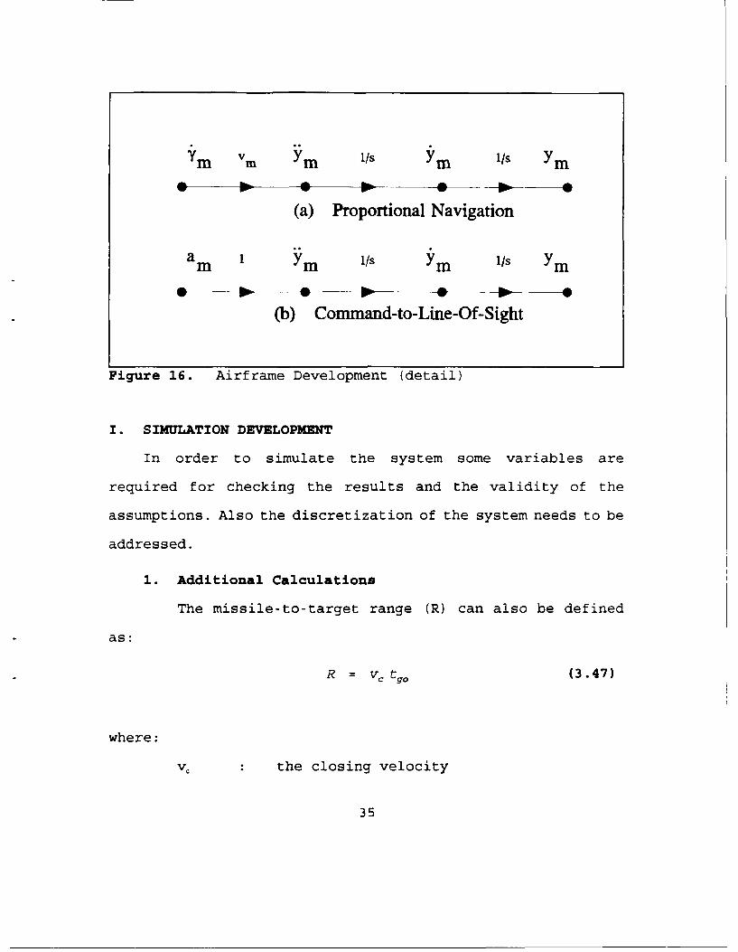
mn m 1 m /S ým 1/s Y
(a) Proportional Navigation
am 1 Ym 1/s Ym 1/s Ym
(b) Command-to-Line-Of-Sight
Figure 16. Airframe Development (detail)
I. SIMULATION DEVELOPMENT
In order to simulate the system some variables are
required for checking the results and the validity of the
assumptions. Also the discretization of the system needs to be
addressed.
1. Additional Calculations
The missile-to-target range (R) can also be defined
as:
R = Vc tgo (3.47)
where:
v, the closing velocity
35
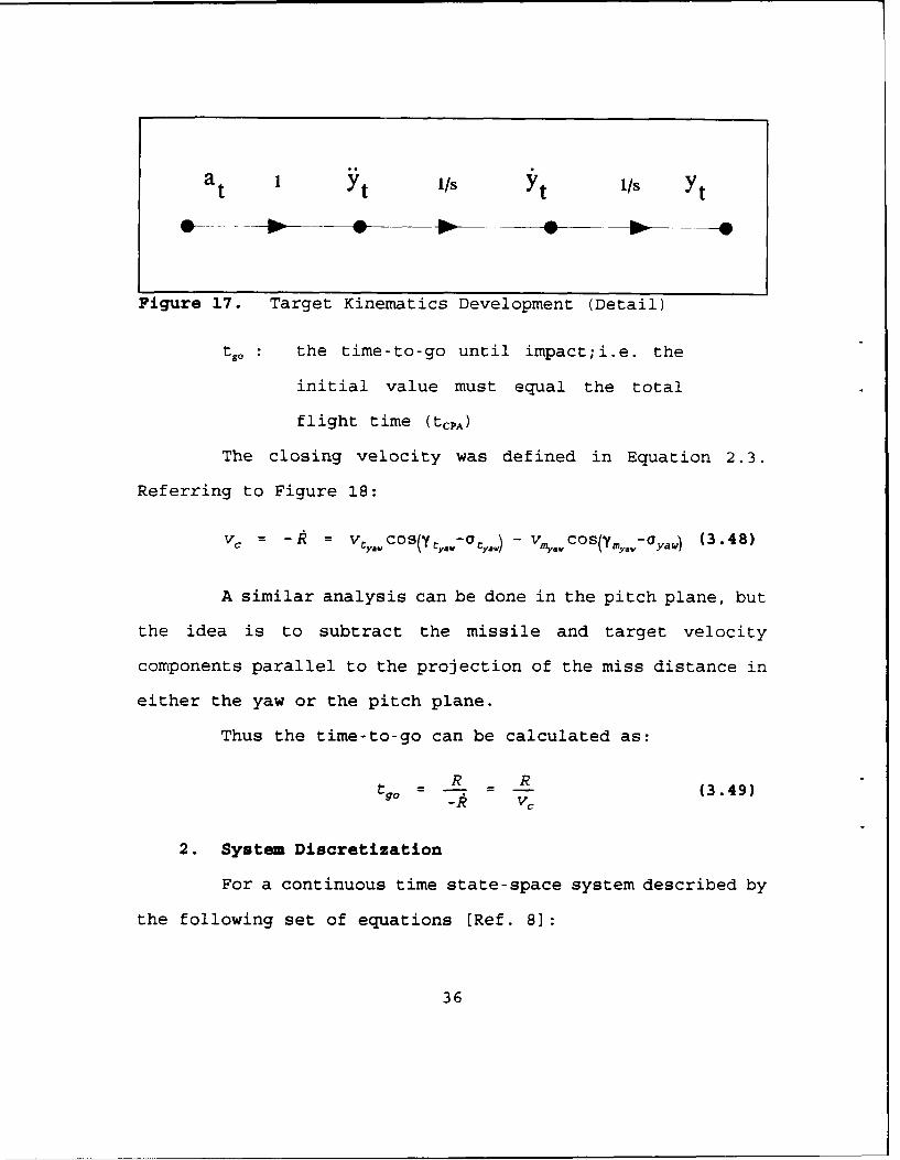
a t Yt /s Y/s Yt
Figure 17. Target Kinematics Development (Detail)
tgo the time-to-go until impact;i.e. the
initial value must equal the total
flight time (tcpA)
The closing velocity was defined in Equation 2.3.
Referring to Figure 18:
v = -R = vtY-vcos(y-tyoCy..) -- v.cos(Ymy-G.jyaw) (3.48)
A similar analysis can be done in the pitch plane, but
the idea is to subtract the missile and target velocity
components parallel to the projection of the miss distance in
either the yaw or the pitch plane.
Thus the time-to-go can be calculated as:
tgo R _ = R (3.49)
2. System Discretization
For a continuous time state-space system described by
the following set of equations [Ref. 81:
36
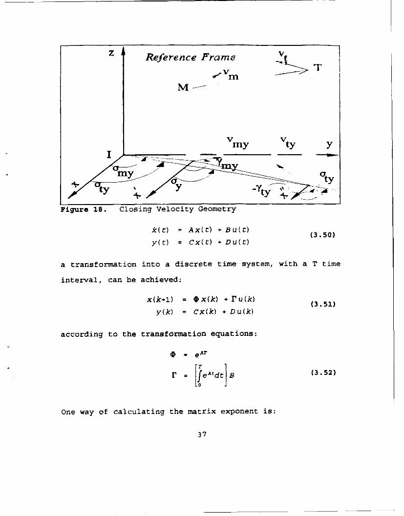
Z Reference Frame V
VV
Vmy tY
Figure 18. Closing Velocity Geometry
*k(t) = Ax(t) +BOO (.50
y(0) = Cx(t) + Du(t)
a transformation into a discrete time system, with a T time
interval, can be achieved:
x(k+l) O x(k) + ru(k) (3.51)
y (k) C Cx(k) + D u(k)
according to the transformiation equations:
*=eAT
r ie JA tdt]IB (3.52)
One way of calculating the matrix exponent is:
37
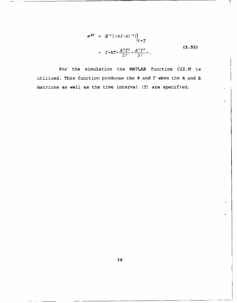
eAT = •-[(sI-A)1 ]I- :T
= 4I+AT+A2 T 2 + A 3 T3 +..
2! 3!
For the simulation the MATLAB function C2D.M is
utilized. This function produces the D and r when the A and B
matrices as well as the time interval (T) are specified.
38
IV. SIMULATION RESULTS
A. OVERVIEW
The computer code for the proportional navigation command
guidance is presented in Appendix 1, and that for the command-
to-line-of-sight in Appendix 2. The assumptions that have been
made throughout will be discussed. The two scenarios run and
their results will also be presented.
B. ASSUMPTIONS
The following assumptions have been made throughout the
analysis and simulation:
"* The missile is not limited in accelerations.
"* The acceleration due to gravity is ignored.
"* The target is capable of instantaneous acceleration.
"* The target has no upper acceleration limit.
"* The proportional navigation constant is 4.
"* The missile is pointed to the target at launch.
C. ENGAGEMENT SCENARIOS
1. Target at Steady, Level Flight
For this scenario the target is flying at a constant
altitude with no acceleration. The missile is fired from the
39
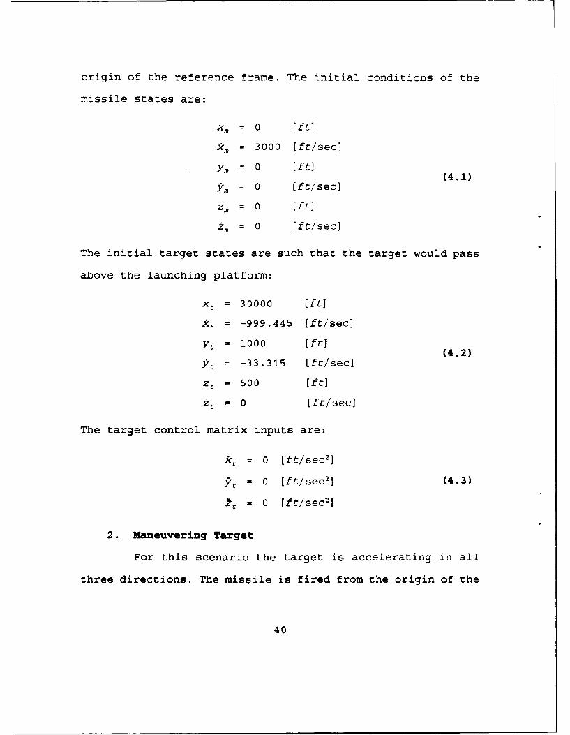
origin of the reference frame. The initial conditions of the
missile states are:
xm, = 0 Ift]
A, = 3000 [ft/sec]
YM = 0 [fft] (4 .1)y' = 0 (ft/sec]
zM = 0 [ift]
z, = 0 [ft/secl
The initial target states are such that the target would pass
above the launching platform:
xt = 30000 [ft]
.kt = -999.445 [ft/secl
yC = 1000 [ft] (4.2)
zt = -33.315 [ft/secl
zt = 500 (ft]
2t = 0 [ft/secl
The target control matrix inputs are:
.R = 0 [ft/sec2]
=t = 0 [ft/sec2 ] (4.3)
2 = 0 [ft/sec2]
2. Maneuvering Target
For this scenario the target is accelerating in all
three directions. The missile is fired from the origin of the
40
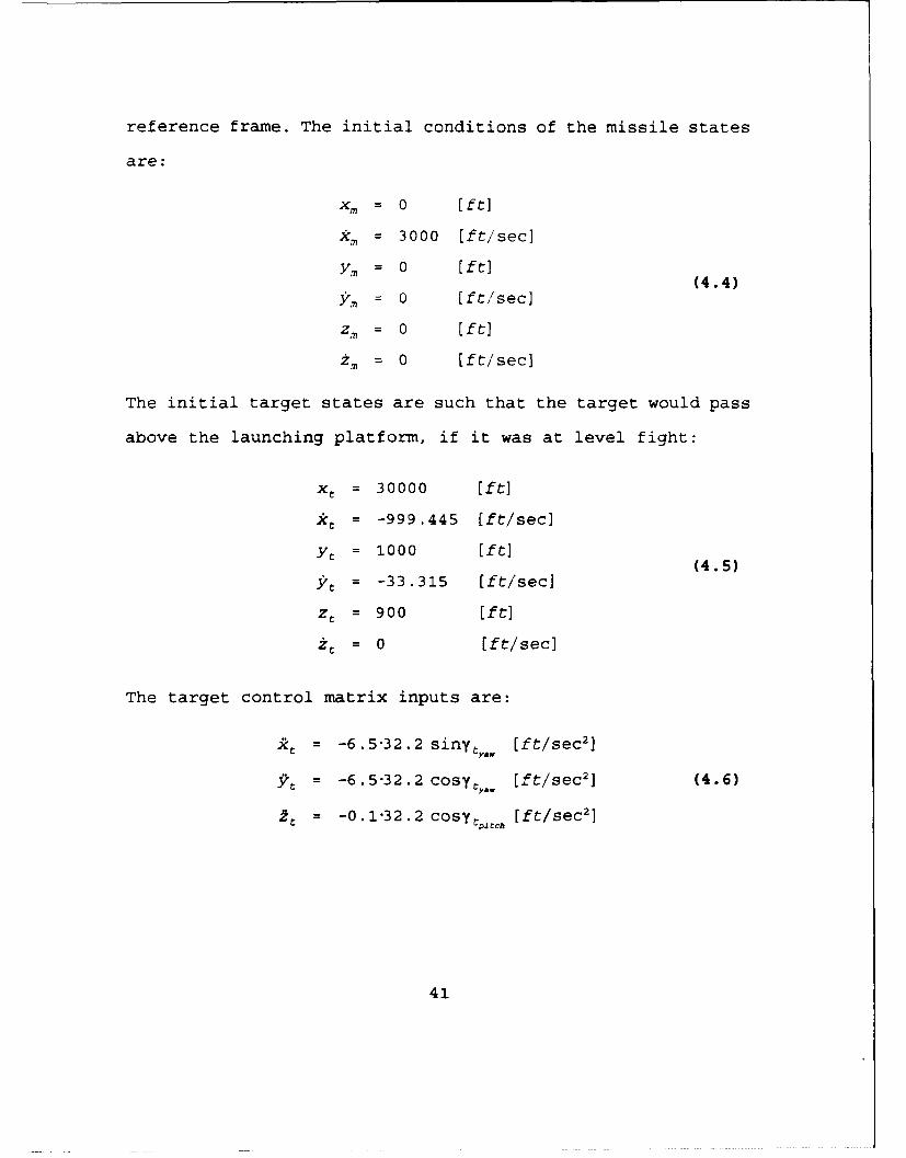
reference frame. The initial conditions of the missile states
are:
Xm = 0 [ft]
km = 3000 [ft/sec]
y.• -- 0 [ift] (4.4)
S% = 0 [ft//sec]
z.? = 0 rft]zI = 0 [ft/sec]
The initial target states are such that the target would pass
above the launching platform, if it was at level fight:
xt = 30000 [ft]
X• = -999.445 [ft/sec]
yr = 1000 [ft] (4.5)Jý = -33.315 [ft/sec]
Zt = 900 [ft]
-+ = 0 [ift/sec]
The target control matrix inputs are:
9t = -6.5-32.2 sinytv," [ft/sec2 ]
St = -6.5.32.2 cosyty,. [ft/sec2 ] (4.6)
= -0.1.32.2 cosy,:, [ft/sec2 ]
41
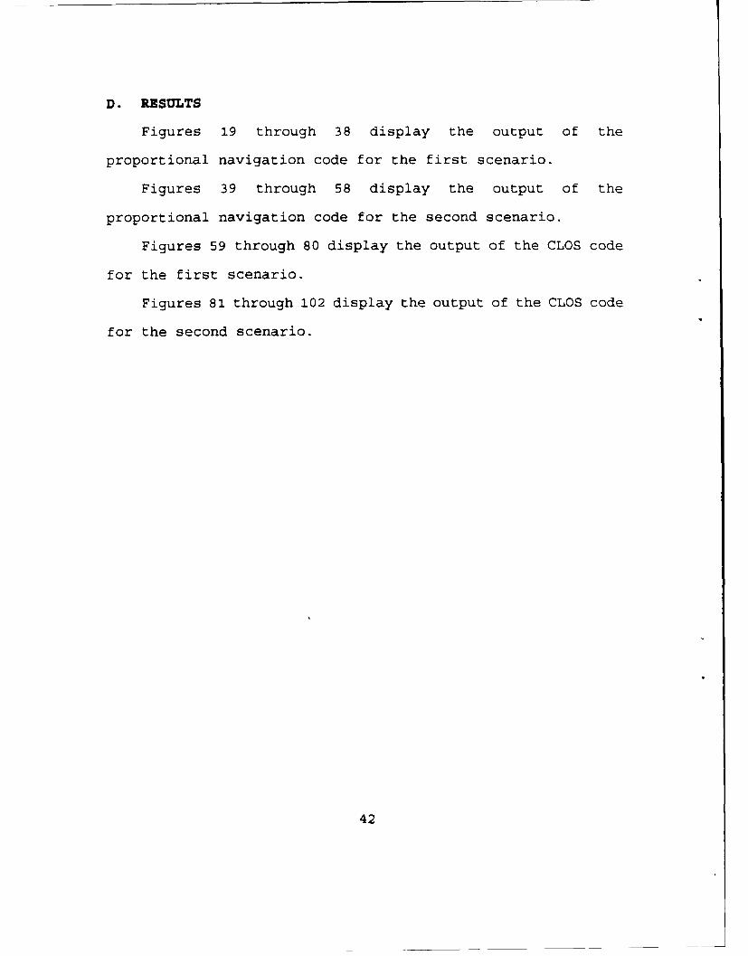
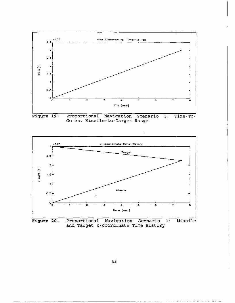
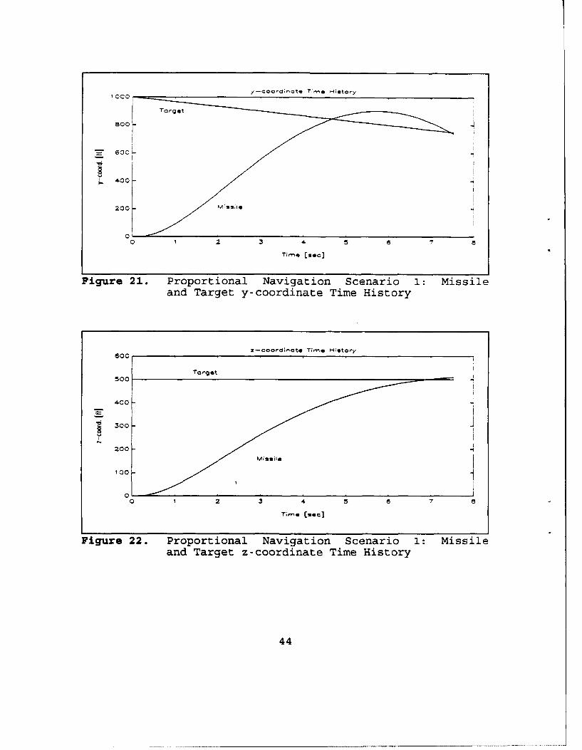
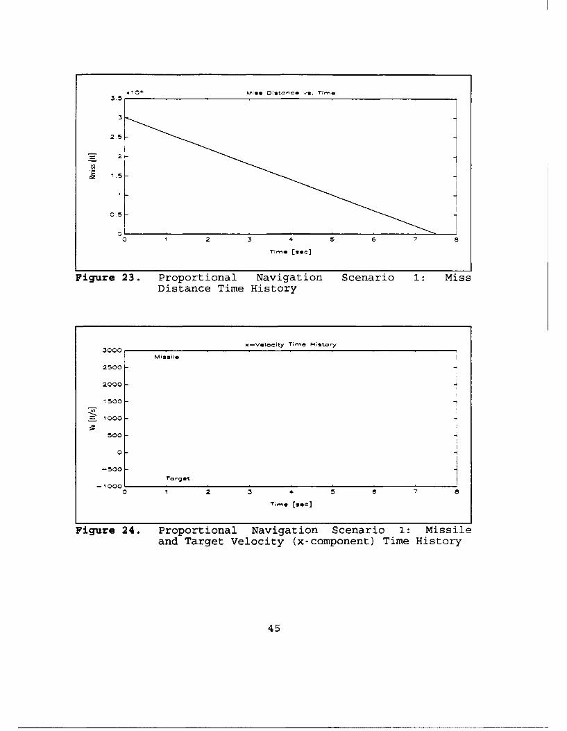
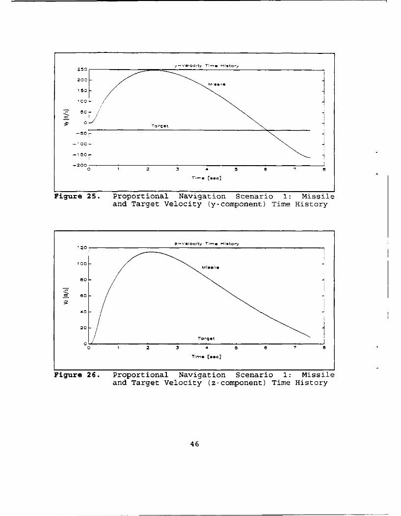
D. RESULTS
Figures 19 through 38 display the output of the
proportional navigation code for the first scenario.
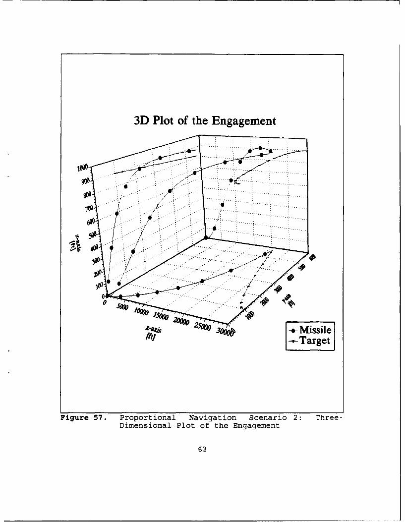
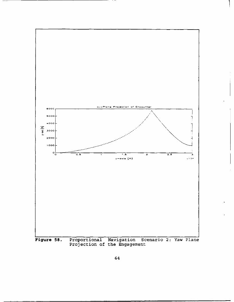
Figures 39 through 58 display the output of the
proportional navigation code for the second scenario.
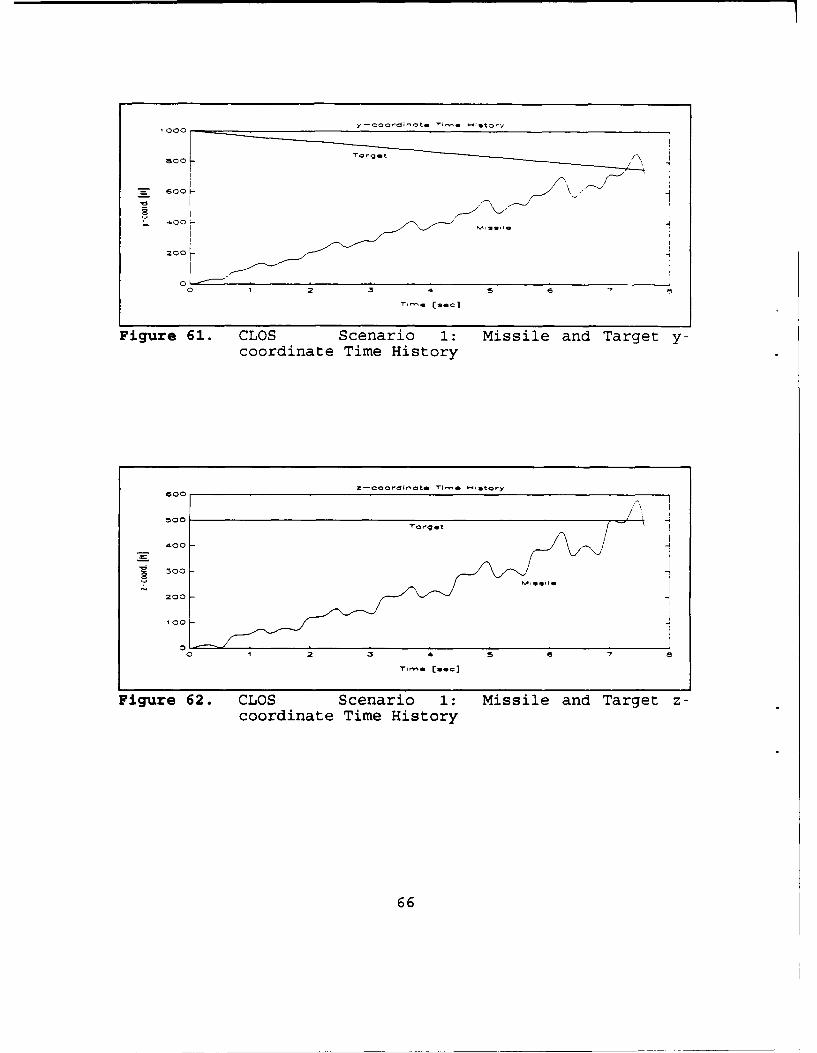
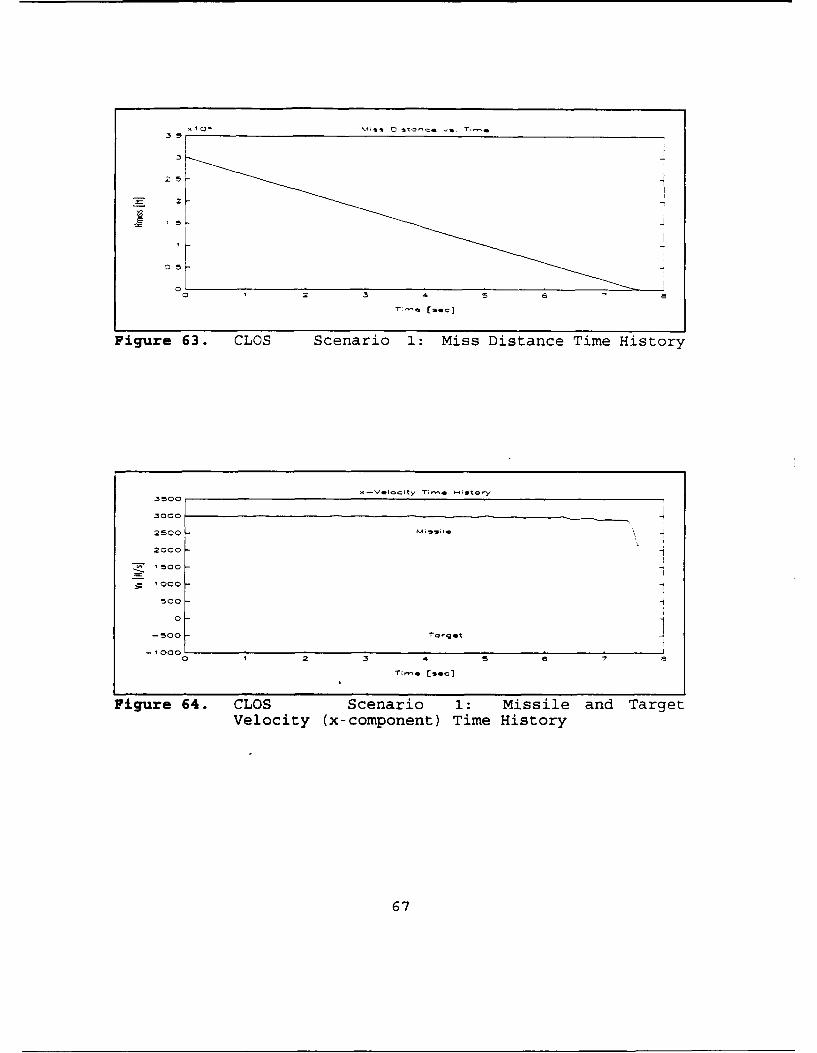
Figures 59 through 80 display the output of the CLOS code
for the first scenario.
Figures 81 through 102 display the output of the CLOS code
for the second scenario.
42
M;32 DivtoCr'e s. T7
re-to-go
1.50.5-0 1 2 3 4 5 6 7 a
'"- [sec]
Figure 19. Proportional Navigation Scenario 1: Time-To-Go vs. Missile-to-Target Range
x 01 x-coordinate Time History3
[ To'get
2.5
2
1.5
0.5
010 1 2 3 4 5 6 7 a
T;.e. [.se]
Figure 20. Proportional Navigation Scenario 1: Missileand Target x-coordinate Time History
43
OCOy de t
Target
"800-
- 60Cr .
S400- ~
200 - MSSil ,
0,0 1 2 4 5 6 7 6
T•me [sac]
Figure 21. Proportional Navigation Scenario 1: Missileand Target y-coordinate Time History
z-coordi•cate Tirme H•story600
500 T
400 j300-
200-Missile
100 i
0012 3 4 e
Figure 22. Proportional Navigation Scenario 1: Missileand Target z-coordinate Time History
44
x 10 Miss OistCce 's. T;•e35
2.5 -
3 2
0.5
0 1 2 3 4 5 6 7 8
Time (sec]
Figure 23. Proportional Navigation Scenario 1: MissDistance Time History
x-Velocity Time History3000
Missile
2500
2000 -
1500-
= 1000--
500-
0 1-500-
-1000 Target0 12 3 4 5 78
Time (see]
Figure 24. Proportional Navigation Scenario 1: Missileand Target Velocity (x-component) Time History
45
V50 .G City Tn-a -;StOr)
2CC -•
501
:•" 0 T<arget
-100 2~I
-200I0 1 2 4 5 6 7
r;me [saec
Figure 25. Proportional Navigation Scenario 1: Missileand Target Velocity (y-component) Time History
z-Velocity T;,e H•story1 20
100
80 -.4
S60
4o 4
20 - /20 Target
0,o 1 2 3 4 5 6 7 6
Tr;-re [sac]
Figure 26. Proportional Navigation Scenario 1: Missileand Target Velocity (z-component) Time History
46
-2. MiSsIe Pitch Angle 's. 7:-e
0.5-
0 2O 12 3 4 5 8 " 8
Time [sec]
Figure 27. Proportional Navigation Scenario 1: MissilePitch Angle Time History
Magfile YO- Angle in. T;l e5
3
2
-- 2
0 1 2 3 4 5 6 7
Time [sac]
Figure 28. Proportional Navigation Scenario 1: MissileYaw Angle Time History
47
Missile Pitch Rate vs. 1.',ae
2.5
2
E 1 FlrE
0~
--0.50 12 3 5 6 7
Th,.e [see]
Figure 29. Proportional Navigation Scenario 1: MissilePitch Rate Time History
MissgIe Yaw R•te vs. Time
2 L
I0o
-1 -4
-20 3 4 5 7
T;m.e [sac]
Figure 30. Proportional Navigation Scenario 1: MissileYaw Rate Time History
48
ciosi~q velocity rS ;-e
4000
2000 ]
_ 0'
-- 000
-2000
-3000-
-400001 2 3 4 5 78
Figure 31. Proportional Navigation Scenario 1: ClosingVelocity Time History
-Ro Zoor Plot
30 125-
= 20 4
15
10
5
017.42 7.44 7.46 7.48 7.5 7.52 7.54 7.56 7.58 7.6 .62
T;me [sec]
Figure 32. Proportional Navigation Scenario 1: MissDistance and Time-of-Closest-Point-of ApproachEnhancement Plot
49
7to•.O mIissil Accelerco•ori /s . Týrýe,
3,50
S 150 -
100
00 1 2 3 4 5 a
Time. Csc]
Figure 33. Proportional Navigation Scenario 1: MissileTotal Acceleration Time History
MissIle x-ACCOIarOtion 'ýg. Tirme5
o - -.
-5
-15
-20
-250 2 3 4 5
Tim. [sac]
Figure 34. Proportional Navigation Scenario 1: MissileAcceleration (x-component) Time History
50
MSSilG Y-ACCOIa rotiO. 's 77*e
300
2501.(\-200-
1 so H
100
E 504-
-150
012 3 4. 5 67"T;,-e ['sac]
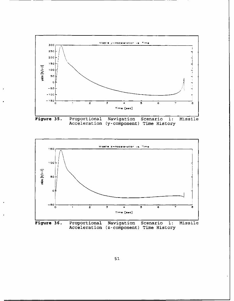
Figure 35. Proportional Navigation Scenario 1: MissileAcceleration (y-component) Time History
MWsole Z-AccaIlOtlOn 9. T;'.
150
100
so-I
0
-50o0 12 3 456 a
Time [sac)
Figure 36. Proportional Navigation Scenario 1: MissileAcceleration (z-component) Time History
51
3D Plot of the Engagement
............... ...............
.. .. .. . .
2ft Missile(~--,-Target
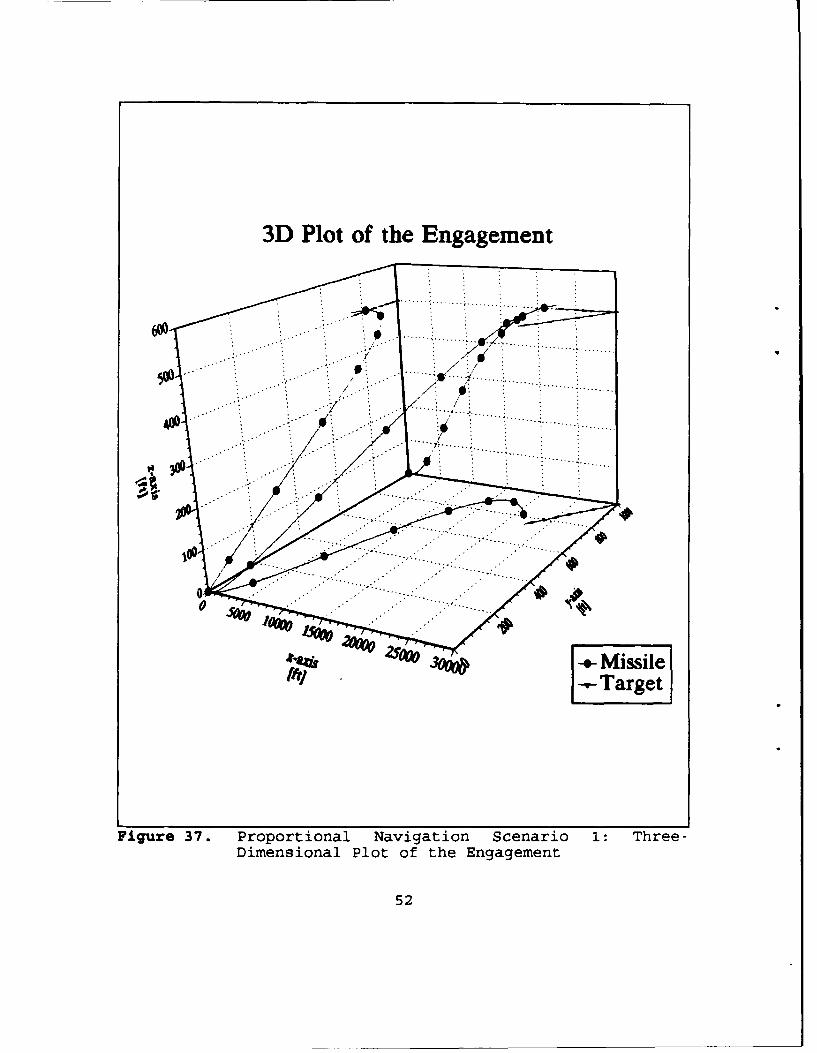
Figure 37. Proportional Navigation Scenario 1: Three-Dimensional Plot of the Engagement
52
lY -'Onft $*,*JQCt~c of EMC-at..t~r1 000
/600 /
I//
200 /
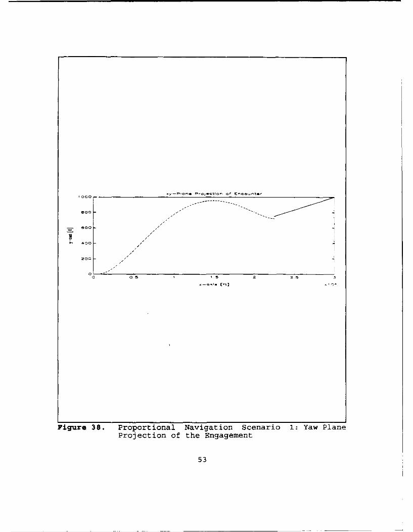
Figure 38. Proportional Navigation Scenario 1: Yaw PlaneProjection of the Engagement
53
2 5
0 5
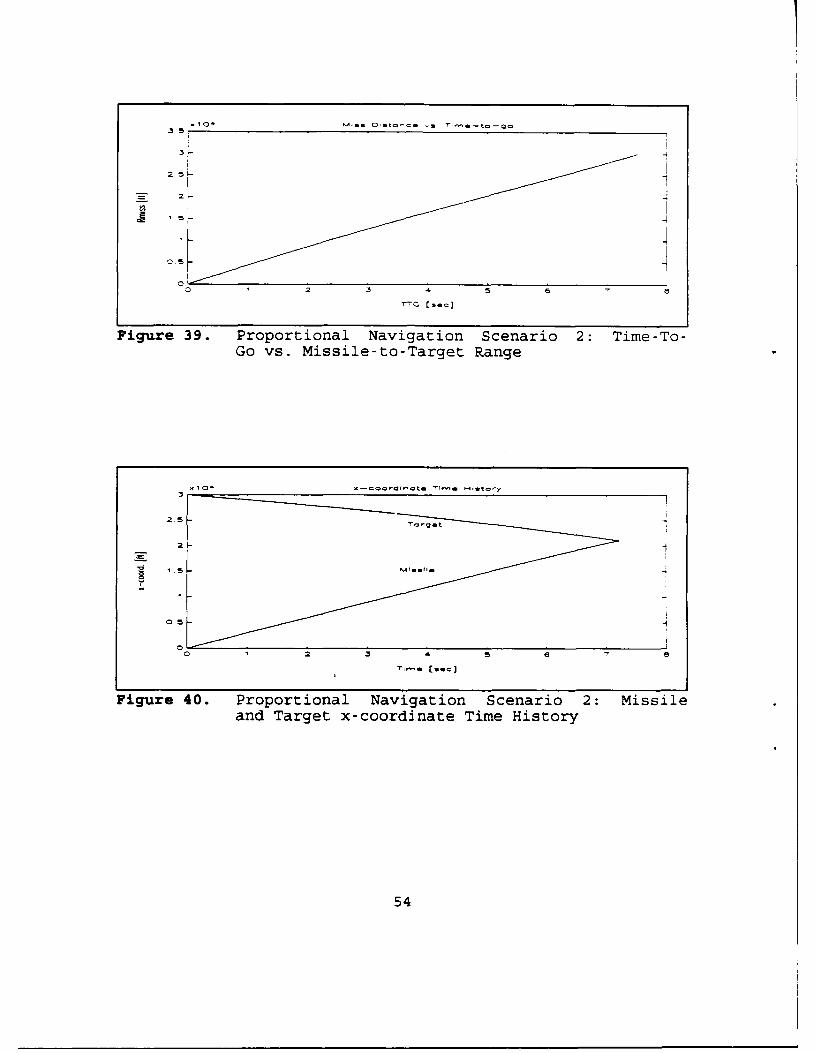
Figure 39. Proportional Navigation Scenario 2: Time-To-Go vs. Missile-to-Target Range
3
25
015 -1
S2 5rr.-,. (.-c
Figure 40. Proportional Navigation Scenario 2: Missileand Target x-coordinate Time History
54
6000 . C Od"t ,--. sa-
- 4[
2000 "i
0 0 'r 2 -3 4"
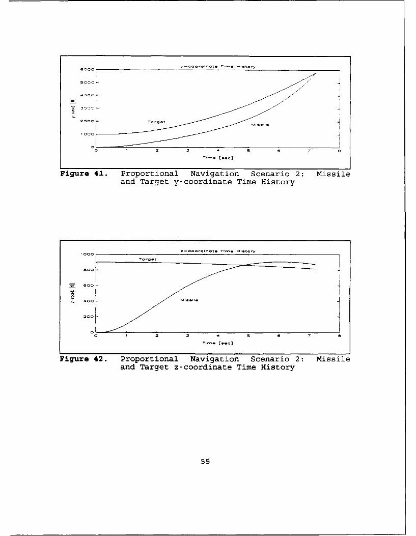
Figure 41. Proportional Navigation Scenario 2: Missileand Target y-coordinate Time History
'000
800-
600 --
200 I
00 2
Ti- w... o [ c]
Figure 42. Proportional Navigation Scenario 2: Missileand Target z-coordinate Time History
55
32
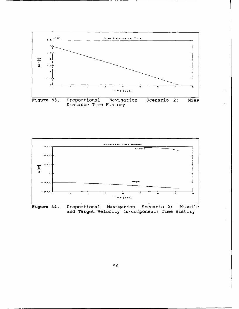
Figure 43. Proportional Navigation Scenario 2: MissDistance Time History
.- V.I..ity Ti-n -4itory3000
2000-~
'_000-
0 -
-1000 r,.
-20000 1 23 78
Ti-o [sec]
Figure 44. Proportional Navigation Scenario 2: Missileand Target Velocity (x-component) Time History
56
3000
2500
0
-500
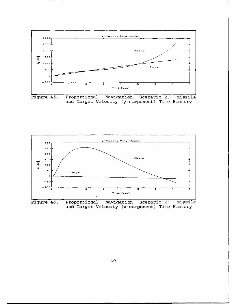
Figure 45. Proportional Navigation Scenario 2: Missileand Target Velocity (y-component) Time History
Z-VaiO-ity Yiwe ý'*-Uoy300
2502
200
150A
'00 -
50
-50-
-100
Tine [sec]
Figure 46. Proportional Navigation Scenario 2: Missileand Target Velocity (z-component) Time History
57
~- 2 / -
1.1'
0 1 2 .34 5 6 "7
T'r e [sec]
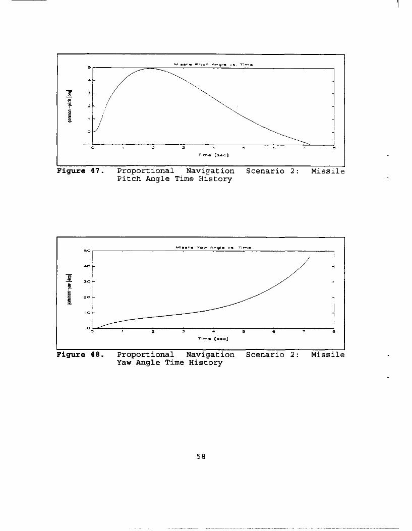
Figure 47. Proportional Navigation Scenario 2: MissilePitch Angle Time History
mIsIIle VCw Antgis vs. T;-*50
.30
20-
10
00 ¶2 3 45 67
TI-se Csec1
Figure 48. Proportional Navigation Scenario 2: MissileYaw Angle Time History
58
25
4]
II
" i 2 4 5 67
Ti-e [sec]
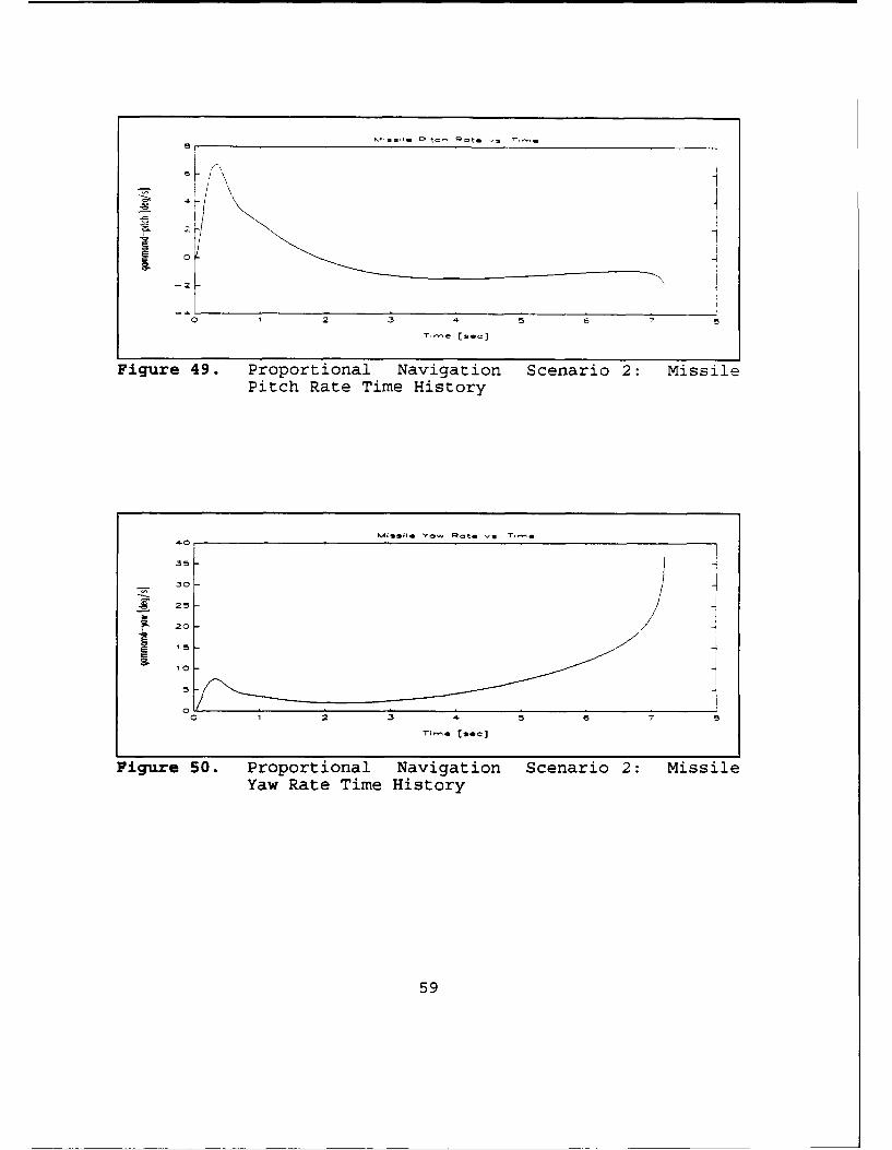
Figure 49. Proportional Navigation Scenario 2: MissilePitch Rate Time History
VI~ss•il YCw at5 vs.
__ 30
_ 25
S' 0
oi ,. s c
Figure 50. Proportional Navigation Scenario 2 : MissileYaw Rate Time History
59
5000
' C
4-4
-2•0000 1 2 3 4 5 6, 7
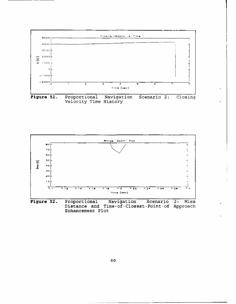
Figure 51. Proportional Navigation Scenario 2: ClosingVelocity Time History
80 H70 -
60
30-20 ,20
7.1 7.12 7.14. 7 16 7.18 7.2 7 22 72ý4 726 7728
Figure 52. Proportional Navigation Scenario 2: MissDistance and Time-of-Closest-Point-of ApproachEnhancement Plot
60
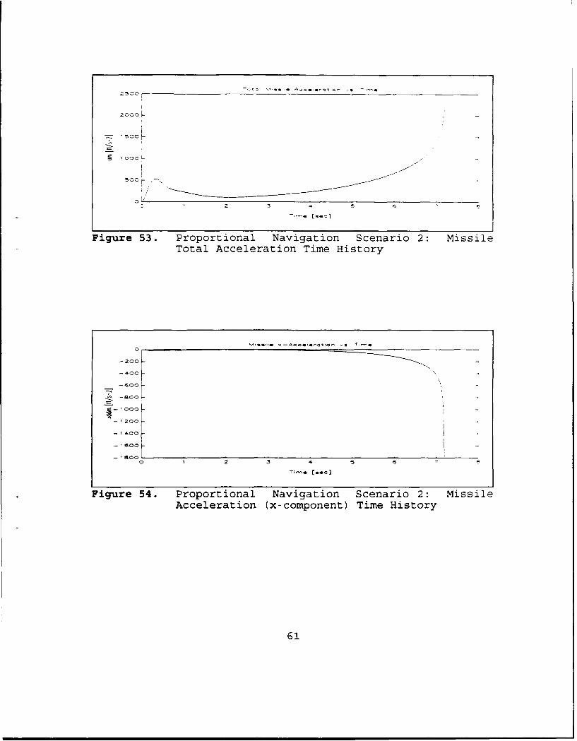
Figure 53. Proportional Navigation Scenario 2: MissileTotal Acceleration Time History
-6 -00
8- 000
So/
a 2 3 4
Figure 54. Proportional Navigation Scenario 2: MissileTotal Acceleration6 Time History-- 661
MsI. ,-AC e..1a, , - ,
1000
- 1 500 2
-500
- 000
0 1 2 3 -. 5 6
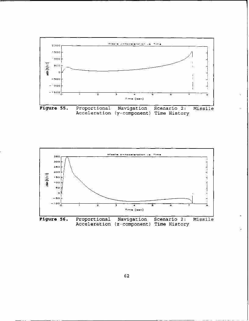
Figure 55. Proportional Navigation Scenario 2 : MissileAcceleration (y-component) Time 1-istory
Mi sH.l z--Acc.Ilertion •v . T;n I
150-
1300
250
__ 200
0
0 1 2 3 5 5 7 5
Ti-*,•e[IC
Figure 56. Proportional Navigation Scenario 2: MissileAcceleration (z-component) Time History
62
3D Plot of the Engagement
: ......... . " " .. . - - , . . . . . . . . . . .. . ..
• . . .i.-" " i~~.. . ..... ....-i '"i...... .. ... . ....... ........ . . "
1k, ' o Missile
Figure 57. Proportional Navigation Scenario 2 : Three-Dimensional Plot of the Engagement
63
40001
5 000-
4.000
2000
1000-
00 0.5 1 1.5 2 2.!S
,x--~ax (pt] - O
Figure 58. Proportional Navigation Scenario 2: Yaw PlaneProjection of the Engagement
64

2 5rzr
o 40 12 35 -
T-rG sc
Figure 59. CLOS Scenario 1: Time-To-Go vs Missile-to-Target Range
0.5
01
Ti-O SaC
Figure 60. CLOS Scenario 1: Missile and Target x-coordinate Time History
65
1000
600
500L
- °-!
zoo-
N' r , 5.I
0 1 2 3 4 5 6 7
"Tir,,s , so[ ]
Figure 61. CLOS Scenario 1: Missile and Target y-coordinate Time History
600 6
4-00
S300
'00 2
0 1 2 .3 4- 5 65 7 6
Figure 62. CLOS Scenario 1: Missile and Target z-coordinate Time History
66
300
04
0 2
00 2 3 5 6 - 6
"rrr• , (sec]
Figure 63. CLOS Scenario 1: Miss Distance Time History
~~x-Velocity xcmoet T;im History.-
3500
3000
5• 00
-500
-- 1000I0 1 2 3 4. 5 6 7
Figure 64. CLOS Scenario 1 : Missile and TargetVelocity (x-component) Time History
67
000
500
-; '
-'000 a 70 ' 2 3 5 67•
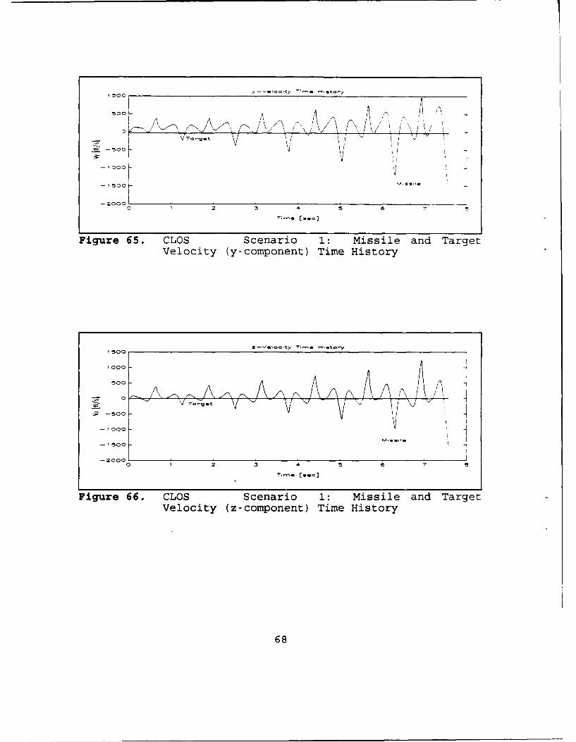
Figure 65. CLOS Scenario 1: Missile and TargetVelocity (y-component) Time History
Z--V.1..ty, Ti-m -+;.toy"1500
1000 -
500
S-500-
-1 500
-2000 01 2 5 ,5 7 1 7
Ti- Cs,• e Sc]
Figure 66. CLOS Scenario 1: Missile and TargetVelocity (z-component) Time History
68
30;
NAsS* .te 4
-g.
20
• - -o - V
-2°
-30
0 1 2 5 4 5 6 -"
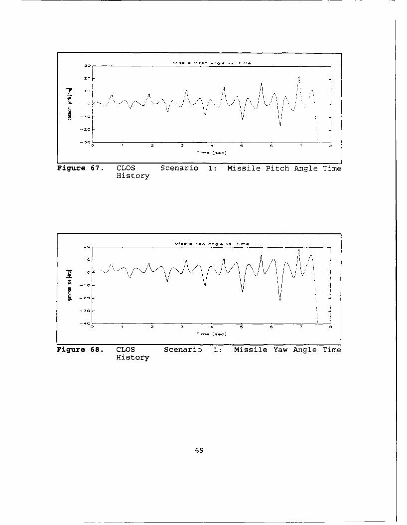
Figure 67. CLOS Scenario 1: Missile Pitch Angle TimeHistory
20
- 0 2~
Figure 68. CLOS Scenario 1: Missile Yaw Angle TimeHistory
69
-4000
3000
2000
- 0'-
-23000
- 3000
--4.0000 1 2 3 4 5 6 7
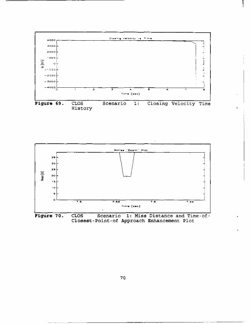
Figure 69. CLOS Scenario 1: Closing Velocity TimeHistory
•l•l Zoo.,," 8lot
35 -130 .425 -
20
° I15 2
7.5 7,55 7. 7.65
Tfre [sac]
Figure 70. CLOS Scenario 1: Miss Distance and Time-of-Closest-Point-of Approach Enhancement Plot
70
2 5r
2 KTif L..c]
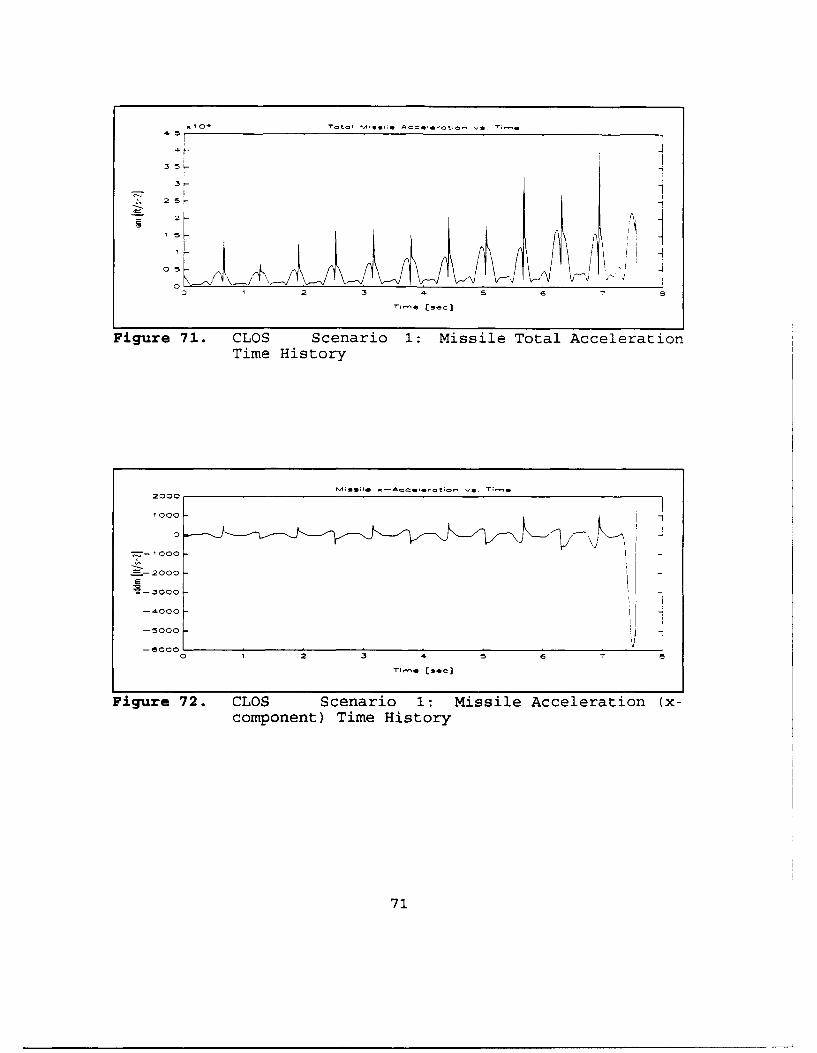
Figure 71. CLOS Scenario 1: Missile Total AccelerationTime History
"Miesil. -a cCIrtr .2000
1 000 I
=2000
- 3000
-6000
Figure 72. CLOS Scenario 1: Missile Acceleration (x-component) Time History
71
2
--2
-- 3 O 1 2 -3 S S S
Ti,-,e (sec]
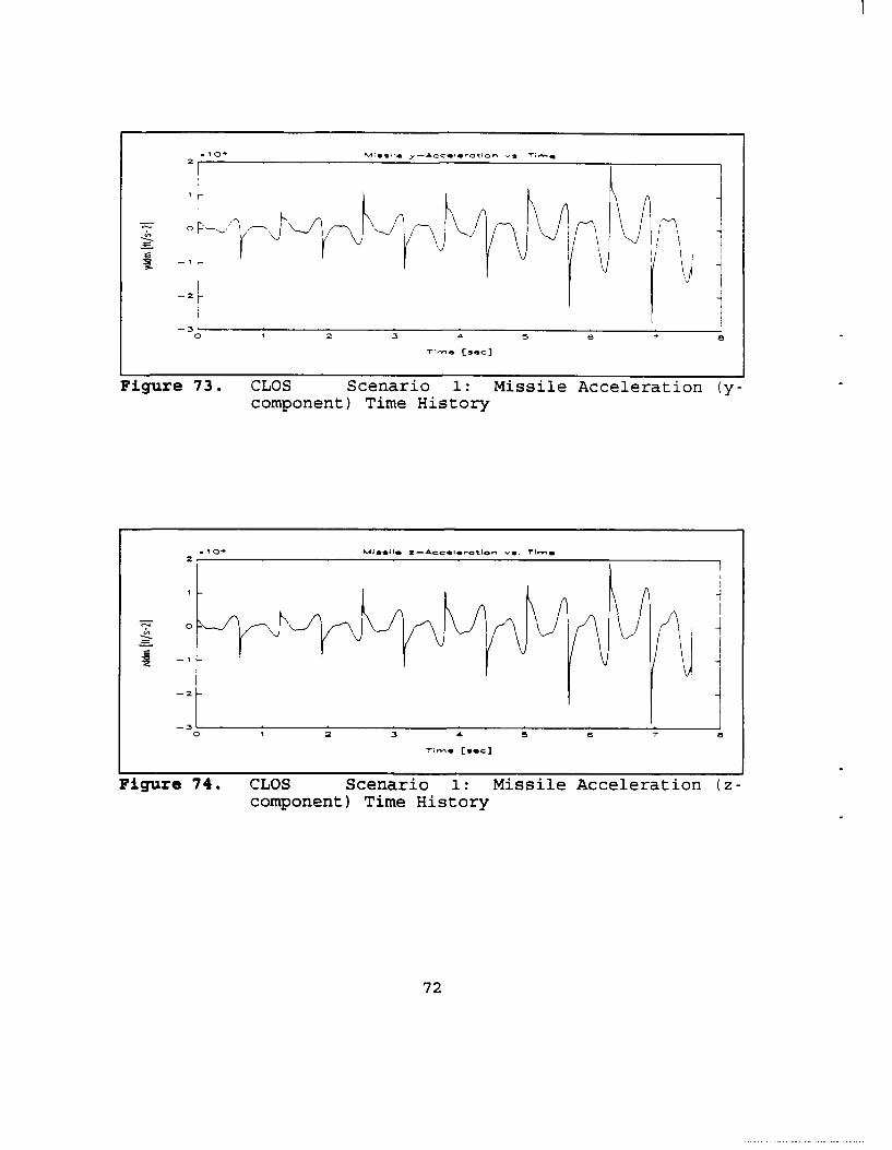
Figure 73. CLOS Scenario 1: Missile Acceleration (y-component) Time History
.•ig ur4eSSI z-ACccIScaai 1 Miss. Aer-
-2
-- 30 1 :2 3 4, 5 6 "7 8
Tin,* o.ec]
Figure 74. CLOS Scenario 1: Missile Acceleration (z-component) Time History
72
3D Plot of the Engagement
...0 . . . .. . ..... ....... ...... ...
i . . . . . . . : :. .. .7 . . . . . . ..S.. .. .... ....
. . . . " :. °. .. . . . . . . . .. .. . . . . . . . . .
0 . . ......
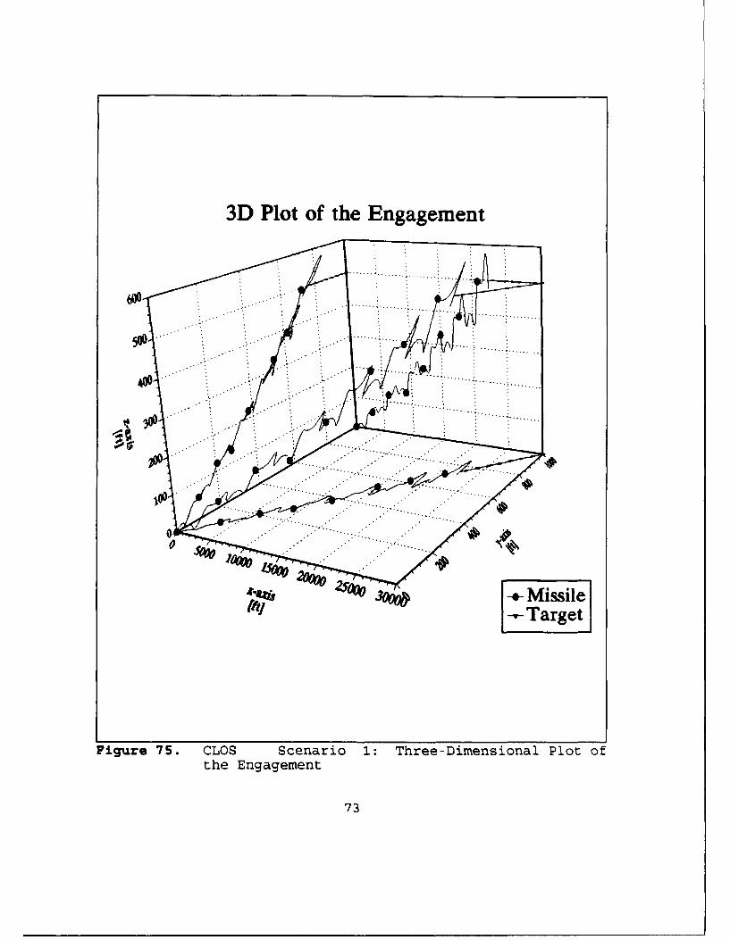
Figure 75. CLOS Scenario 1: Three-Dimensional Plot ofthe Engagement
73
1000
600 4
400 7,I
200 20-
00.5 ¶ 5 2 2.5
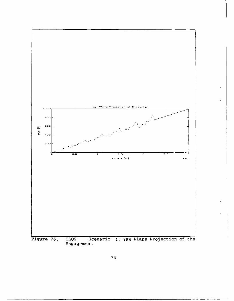
Figure 76. CLOS Scenario 1: Yaw Plane Projection of theEngagement
74
100
II
-- '500 ' 2 3 4 5 6 -
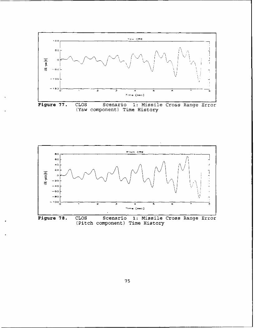
Figure 77. CLOS Scenario 1: Missile Cross Range Error(Yaw component) Time History
80 i 220
0
-20-
-~0
-60 '-80 4I
-- 100
0 1 2 3 4 5 6 7 5
Ti-e LSac]
Figure 78. CLOS Scenario 1: Missile Cross Range Error(Pitch component) Time History
75
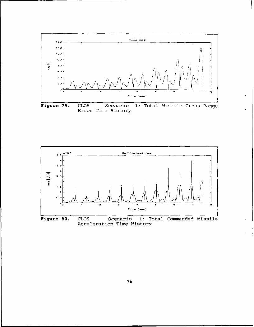
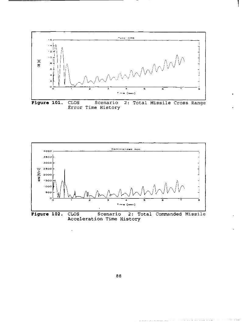
rtotl GRE
160
1400
20 /
/,] fYI
1 5
0 4
2, -
Figure 80. CLOS Scenario 1: Total Commanded MissileAcceleration Time History
76
05-
T-rG [see]
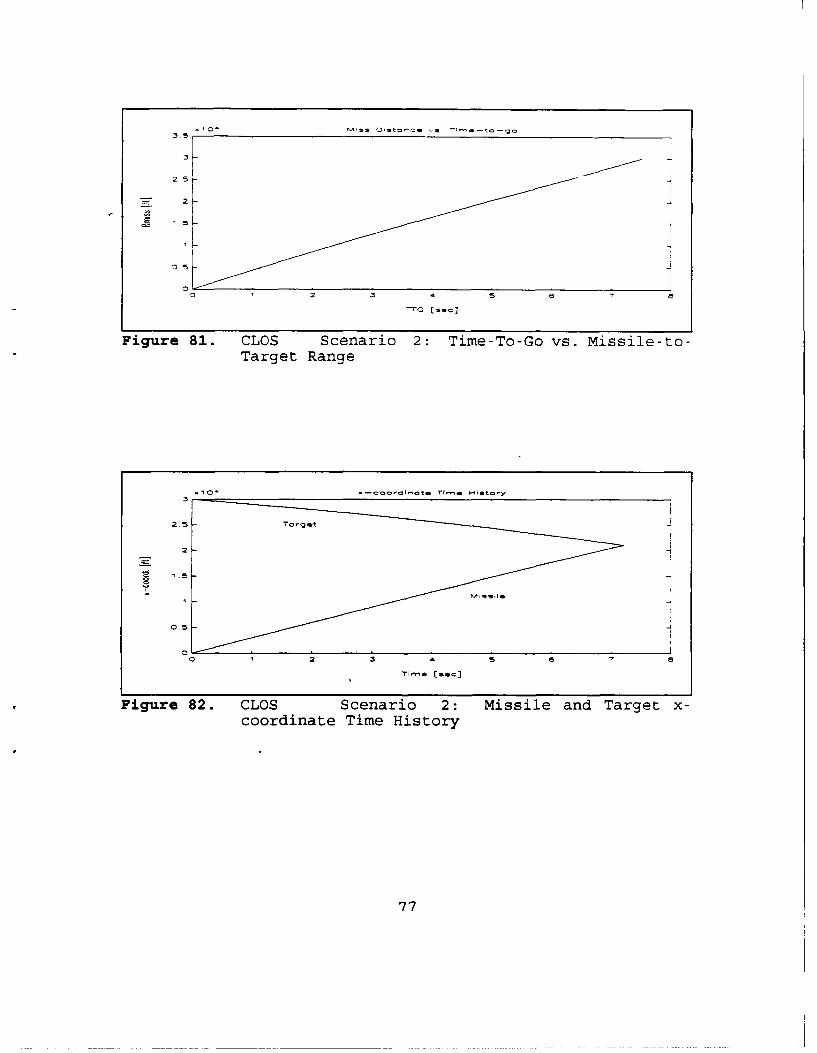
Figure 81. CLOS Scenario 2: Time-To-Go vs. Missile-to-Target Range
I 01 •- - cClrdm ot. T~m. HI- to•y
31
2
0 12 5456
Figure 82. CLOS Scenario 2: Missile and Target x-coordinate Time History
77
5000
2000
t000 lH
01 3 4 S 6 7 2
Ti-e (see]
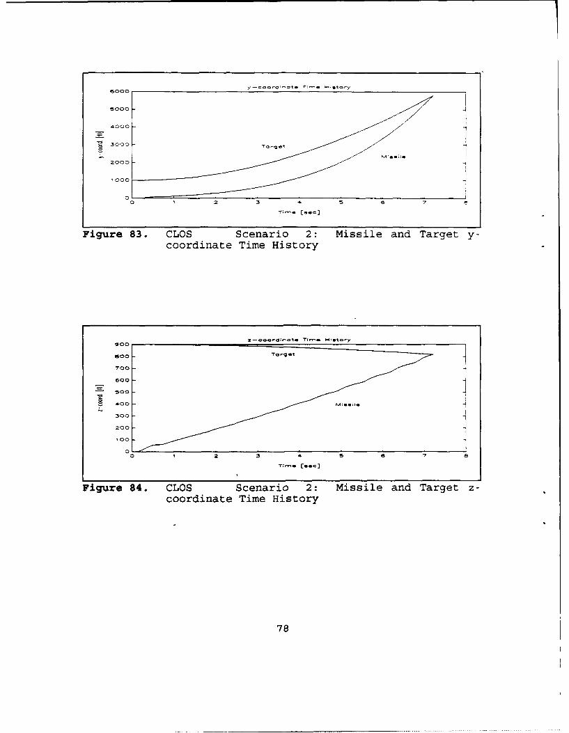
Figure 83. CLOS Scenario 2: Missile and Target y-coordinate Time History
2- roordi- te 1 Il4itary
700 -.
300 1
200 ~,00 -
0 1 2 3 4 5 a 7 a
Figure 84. CLOS Scenario 2: Missile and Target z-coordinate Time History
78
2 5
2
a 5Q •2 3 6 -
"r;r,-.- s. cJ[ee
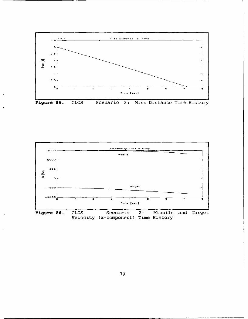
Figure 85. CLOS Scenario 2: Miss Distance Time History
3000
2000
S1000
1:::
-- 200H0 45 7
Figure 86. CLOS Scenario 2: Missile and TargetVelocity (x-component) Time History
79
2500
2000-
1500
1001-500
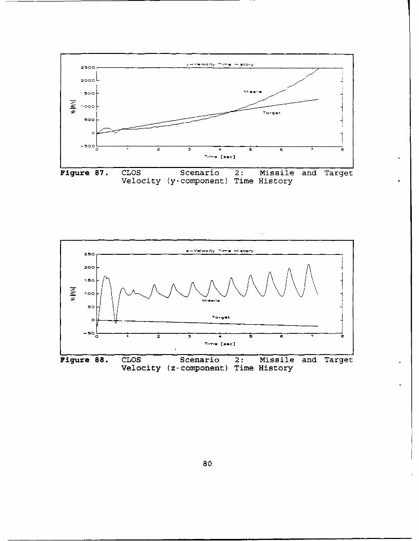
Figure 87. CLOS Scenario 2: Missile and Target.velocity Cy-component) Time History
S-vmIOCity nfl-. 1-iftt.rY250
200-
150 j
100-
50-
-50
TI-l* s J
Figure 88. CLOS Scenario 2: Missile and TargetVelocity (z-component) Time History
80
5 15
'. ' 'r \, '\ i ,
! , // ,\ '
2
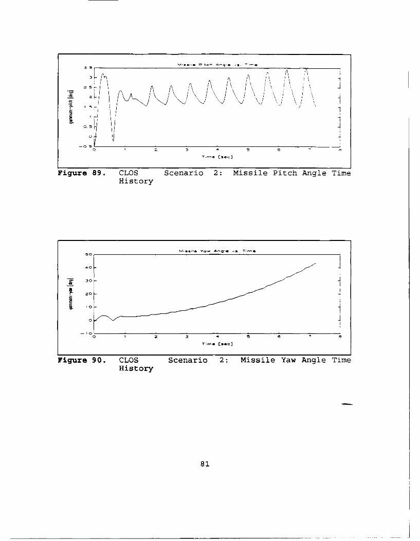
Figure 89. CLOS Scenario 2: Missile Pitch Angle TimeHistory
&4mgiIC V0
• Angle ve
50
20 --
30
20
0 22
Figure 90. CLOS Scenario 2: Missile Yaw Angle TimeHistory
81
. i.. .... ....
3000
4000
3000
2000
'1000
-- 000 -
-2000 -4
- 3000
-4000 0 I 2 3 S 8 7
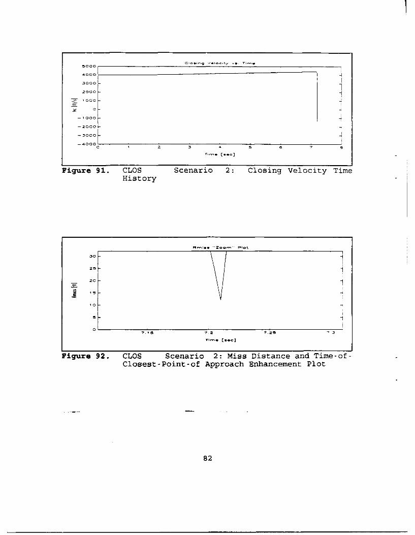
Figure 91. CLOS Scenario 2: Closing Velocity TimeHistory
RmiCC "Zoom" RIot
30
25 1
20 -
15
10
7.15 7 2 7.25
T,•e [90c)
Figure 92. CLOS Scenario 2: Miss Distance and Time-of-Closest-Point-of Approach Enhancement Plot
82
35°C - -i30 C0 -
-
- 2500"-300 \
5CC JVJ
C3 4 6 7
"r, -re [sac]
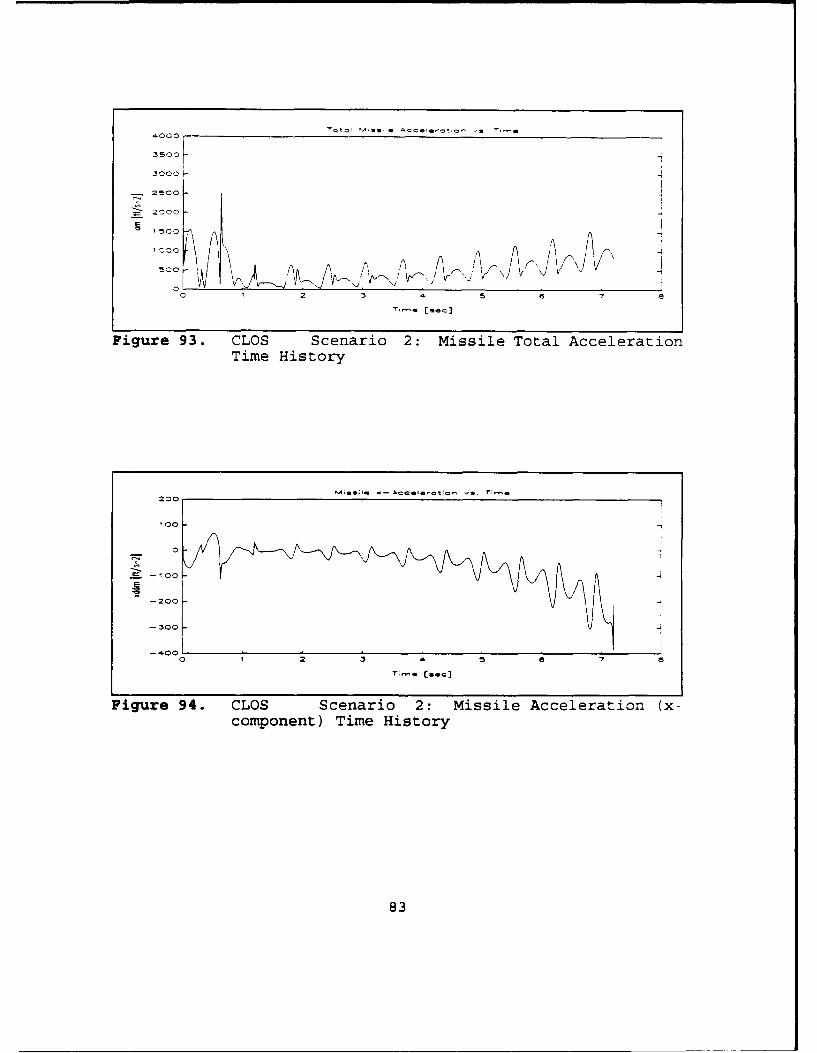
Figure 93. CLOS Scenario 2: Missile Total AccelerationTime History
x-- *cTec;o- ',
- 200
-300 -J
0 1 2 35 7
Ti-a Csoc]
Figure 94. CLOS Scenario 2: Missile Acceleration (x-component) Time History
83
2000
0 0 0
A -,
•- Z1 A
-2000-
- 30000 1 2 34 6 7 6
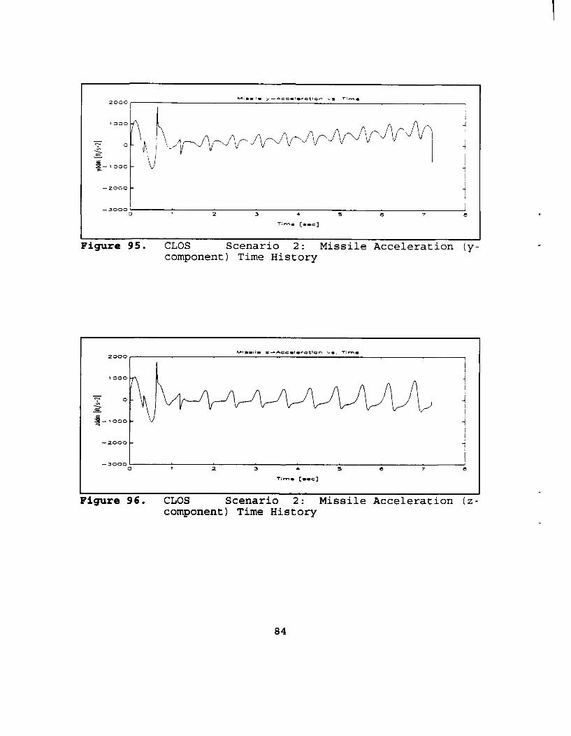
Figure 95. CLOS Scenario 2: Missile Acceleration (y-component) Time History
hAI~aII*II t-ACCe~*rO•tbnv •. ""
2000
1000
So0
- 000
-2000-
-3000
"?r,,e [..e1
Figure 96. CLOS Scenario 2: Missile Acceleration (z-component) Time History
84
3D Plot of the Engagement
............................... ......
Owl~
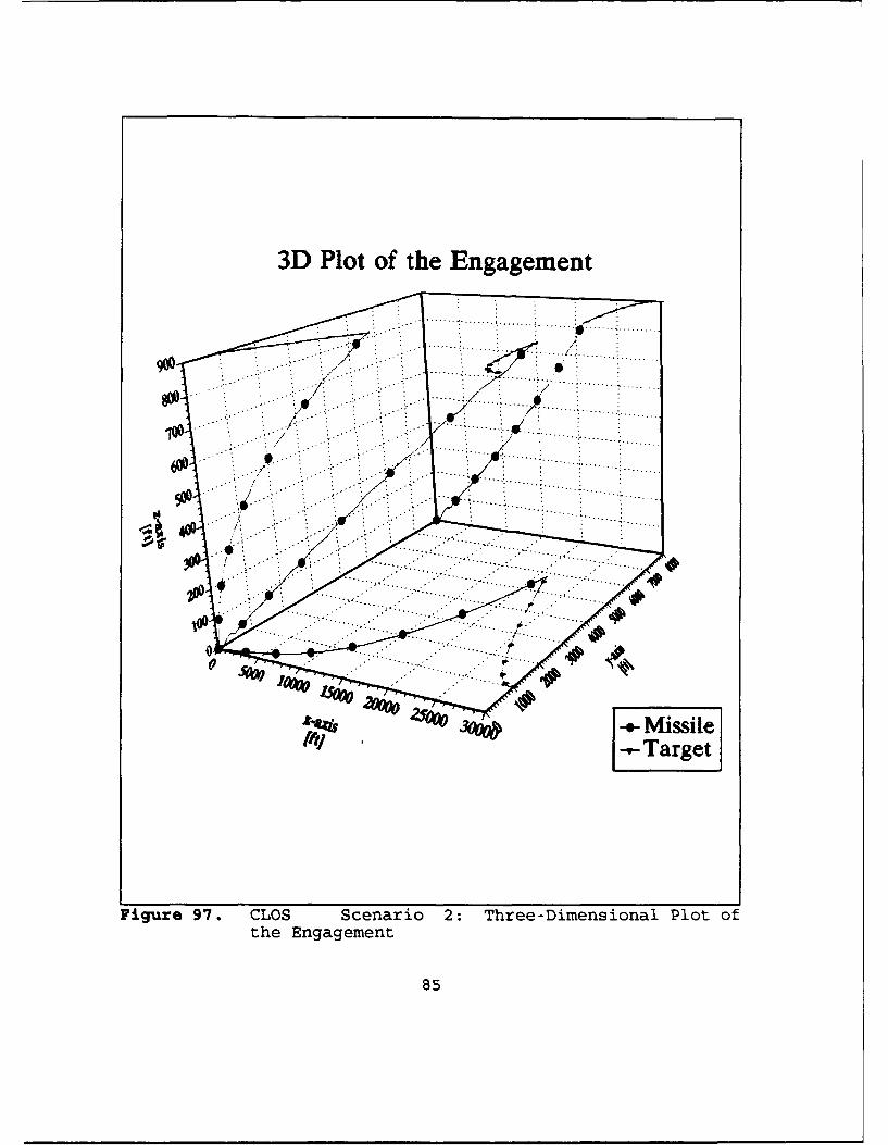
Figure ~ ~ ~~ .. 97. ...S Scnai.2.Tre-imnioalPotothe... Engagement
60D .5
6.000
5000
/"4000/
-000 /
3000o
0 0,5 1,5 2 2.5 3
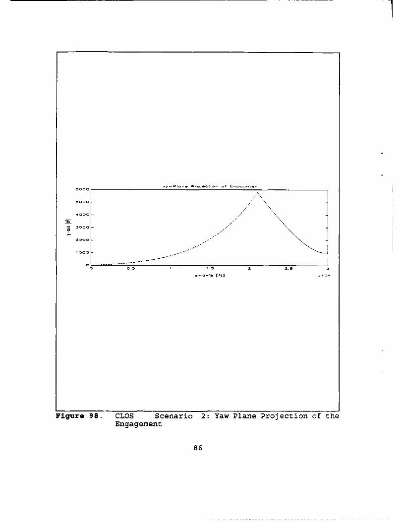
Figure 98. CLOS Scenario 2: Yaw Plane Projection of theEngagement
86
3t
3 5
-10 0 ,' 2 5 6
"~rre [s,.e]
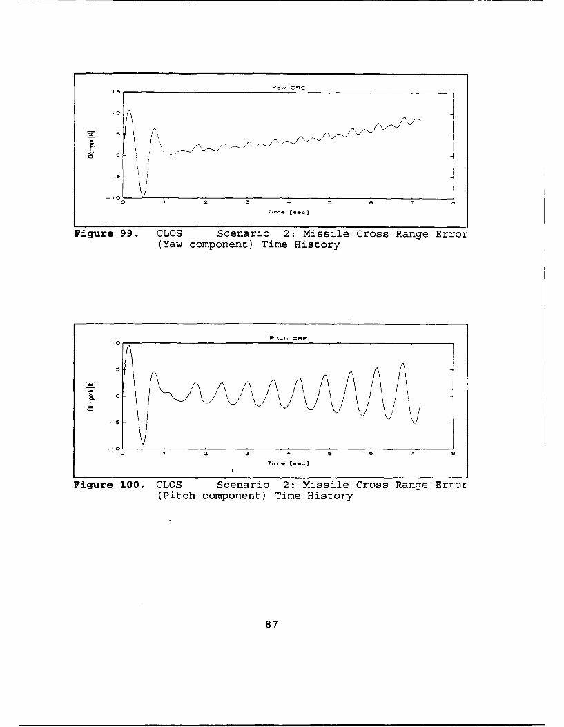
Figure 99. CLOS Scenario 2: Missile Cross Range Error(Yaw component) Time History
8Ftc7 C7 E
-5
-10o0 1 2 3 4 5 6 7 6
Figure 100. CLOS Scenario 2: Missile Cross Range Error(Pitch component) Time History
87
2 2
-00
200
10001
3500
C00 -
Figure 102. CLOS Scenario 2: Total Commanded MissileAcceleration Time History
88
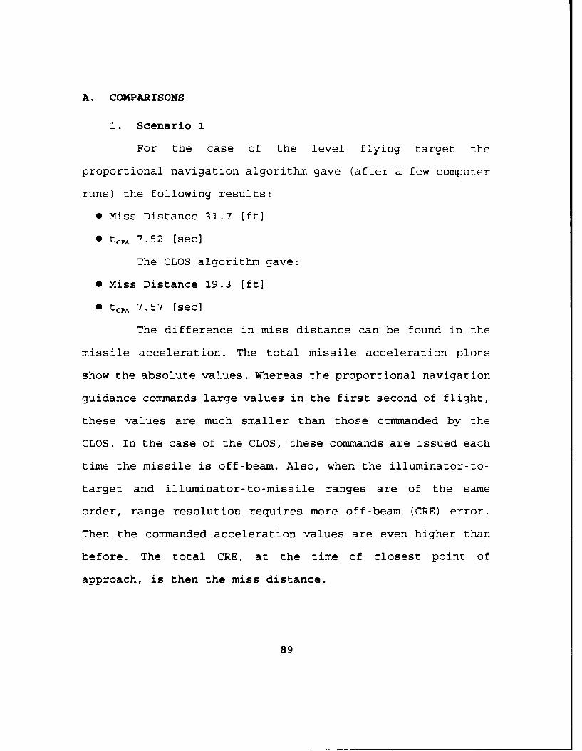
A. COMPARISONS
1. Scenario 1
For the case of the level flying target the
proportional navigation algorithm gave (after a few computer
runs) the following results:
"* Miss Distance 31.7 [ft]
" tcpA 7.52 [sec]
The CLOS algorithm gave:
"* Miss Distance 19.3 [ft]
" tcpA 7.57 [sec]
The difference in miss distance can be found in the
missile acceleration. The total missile acceleration plots
show the absolute values. Whereas the proportional navigation
guidance commands large values in the first second of flight,
these values are much smaller than those commanded by the
CLOS. In the case of the CLOS, these commands are issued each
time the missile is off-beam. Also, when the illuminator-to-
target and illuminator-to-missile ranges are of the same
order, range resolution requires more off-beam (CRE) error.
Then the commanded acceleration values are even higher than
before. The total CRE, at the time of closest point of
approach, is then the miss distance.
89
There is no distinct difference in the total flight
time, but all computer runs showed a consistent lower flight
time for the proportional navigation guidance in the order of
hundredth of a second.
2. Scenario 2
For the case of the maneuvering target the
proportional navigation algorithm gave (after a few computer
runs) the following results:
"* Miss Distance 63.4 [ft]
" tCpA 7.20 [secl
The CLOS algorithm gave:
"* Miss Distance 12.1 [ft]
"* tcPA 7.21 (sec]
The same miss distance analysis, outlined in the
previous subsection, holds here also. But in this case, the
proportional navigation guidance gives a much higher miss than
that of the CLOS.
The large acceleration demands impose large pitch and
yaw angles. These, in turn, modify the velocity vectors, and
finally the trajectory.
90
V. CONCLUSIONS AND RECOMMENDATIONS
A. CONCLUSIONS
Although the proportional navigation scheme may be an
excellent tool for inertial guided missiles, command guidance
offers attractive alternates.
In the case of beam riding, the missile does not require
a seeker, thus reducing the unit production cost. On the other
hand, the illuminator is required to remain occupied with the
target until intercept. Also the accuracy varies inversely
proportional with the range of intercept;i.e. targets engaged
close to the illuminator produce higher range resolution than
targets further away.
The algorithms developed provide an insight to the two
different guidances. Proportional navigation gave higher miss
distances as the target increased its maneuverability, whereas
CLOS remained consistent throughout.
B. RECOMMENDATIONS
The application of an acceleration limit, would be an easy
addition to the algorithms and would provide further insight
to the comparison.
91
The implementation of noise in the measured angles, would
further approximate real world conditions.
A Monte Carlo statistical analysis, would provide a
further insight to the accuracy of the results.
Finally, an adjoint model analysis, would provide an
excellent result validation tool.
92
APPENDIX A - PROPORTIONAL NAVIGATION CODE
%Title Three (3) dimensional Command
%1 Guidance (PN)
%Author Dimitrios Peppas
%Date 10/01/92
%Revised 12/01/92
%Project Thesis
%System Legend 386SX
%Compiler 386 - MATLAB v.: 3.5m
%Description : This code solves a 3D target/missile
%- problem using a proportional navigation
%1 command guided missile (Forward Time
t Model).
clg
clear
!del cg*.met;
!del cg3dm.dat;
!del cg3dt.dat;
clc
runtime=clock; %Initialization for calculation of runtime
rtod=180/pi; %Rad-to-Degree Conversion factor
flops(0); %Reset Floating Point Operations Counter
93
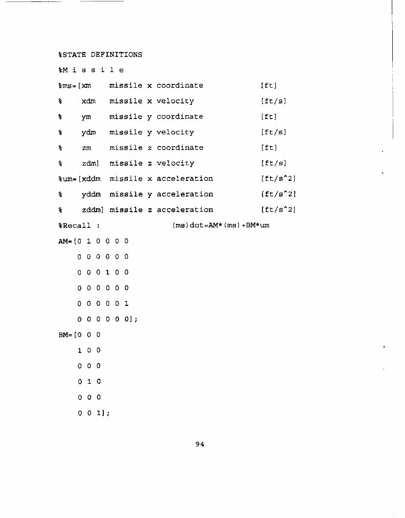
%STATE DEFINITIONS
%M i s s i1 e
%ms=[xm missile x coordinate [ft]
S xdm missile x velocity [ft/s]
YM missile y coordinate [ft]
ydx missile y velocity [ft/si
% zm missile z coordinate [ft]
k zdm] missile z velocity [ft/s]
%um=[xddm missile x acceleration [ft/s-2]
yddm missile y acceleration [ft/sA2]
zddm] missile z acceleration [ft/sA2]
%Recall : (ms)dot=AM*(ms)+BM*um
AM=[O 1 0 0 0 0
000000
000100
000000
000001
0 0 0 0 0 0];
BM=[0 0 0
100
000
0 1 0
000
0 0 1];
94

%T a r g e t
%ts=[xt target x coordinate [ft]
% xdt target x velocity [ft/si
yt target y coordinate [ft]
ydt target y velocity [ft/s]
zt target z coordinate [ft]
zdt] target z velocity [ft/s]
%ut=[xddt target x acceleration [ft/sA2]
% yddt target y acceleration [ft/sA2]
% zddt] target z acceleration [ft/sA2]
%Recall (ts)dot=AT*(ts)+BT*ut
AT=AM;
BT=BM;
%-Time and Navi ga t i on Cons t ant s
%ttrack F.C.S. tracking constant [sec]
%tmc F.C.S. missile command constant [sec]
%N F.C.S. Navigation constant [dimensionless]
ttrack=0.1;
tmc=l;
N=4;
kl=(l/ttrack) A2;
k2= (2/ttrack)
k=(l/tmc);
%F.C.S. T r a c k e r a n d F i 1 t e r
95
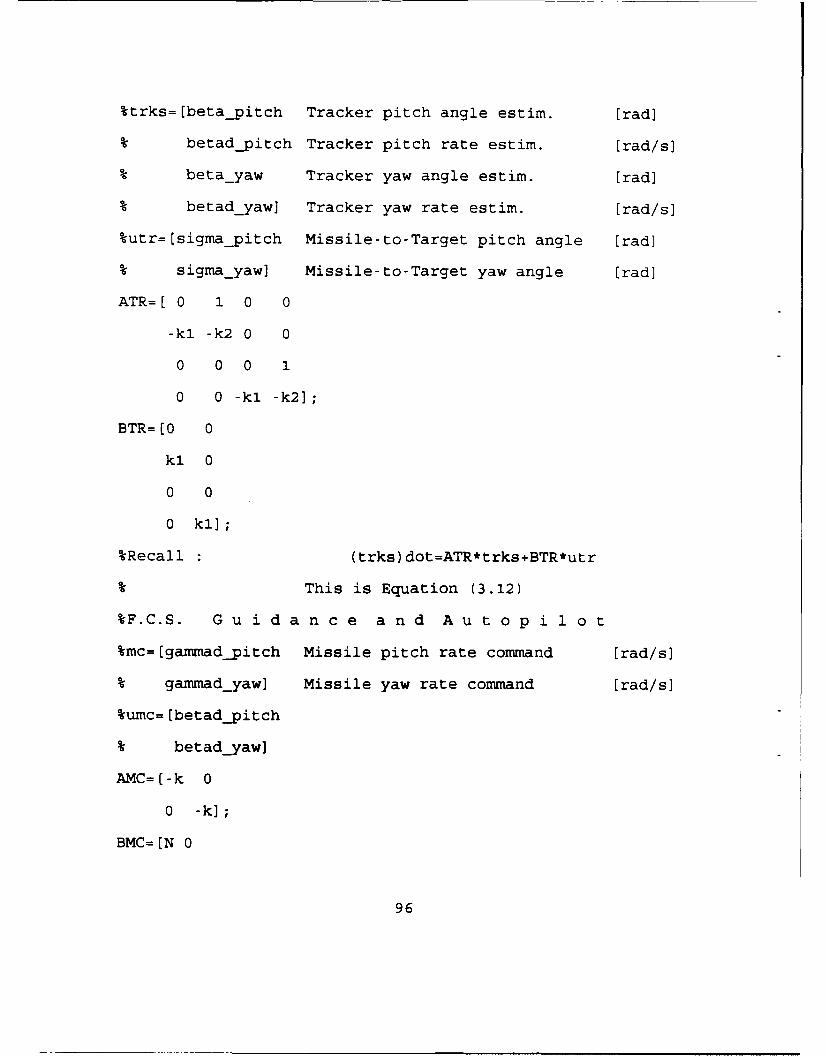
%-trks=[beta~pitch Tracker pitch angle estirn. [rad)
W betad-pitch Tracker pitch rate estim. [rad/s]
06 beta yaw Tracker yaw angle estim. [rad]
16 betad yawl Tracker yaw rate estim. [rad/s]
%utr=[sigma~pitch Missile-to-Target pitch angle [rad]
P6 sigma yaw] Missile-to-Target yaw angle [rad]
ATR=[ 0 1 0 0
-kl -k2 0 0
0 0 0 1
0 0 -ki -k2];
BTR=[0 0
ki 0
0 0
0 kil;
%Recall (trks) dot=ATR*trks.,BTR*utr
% This is Equation (3.12)
%F.C.S. G u id a nce a nd Au to p ilo t
%-mc=[gammad~pitch Missile pitch rate command [rad/si
P6 ganimad yaw] Missile yaw rate command [rad/sI
%-umc= [betad~pitch
P6 betad~yaw]
AMC=[-k 0
0 -k];
BMC=[N 0
96
0 N];
%Recall (mc) dot=AMVC*mc+BMC*urnc
?k This is Equation (3.30)
tD i s c r e t i z a t i o n
dt=. 01; tIntegration Interval [sec]
[phim,delml =c2d(AM,BM,dt);
fphit,delt]=c2d(AT,BT,dt);
[phitr,deltr] =c2d(ATR,BTR,dt);
Ilphimc,delmc] =c2d(AMC,BMC,dt);
tfinal=l5.0; tCalculation time range [sec]
kmax=tfinal/dt+l; %Maximumn main loop runs
%I n i t i a 1 i z a t i o n
ms(:,l)=[ 0
3000
0
0
0
0 1
ts (:1) ( 30000
-999.445
1000
-33.315
500
0 1
97
trks (: , 1) = [0
0
0
0]
mc (: 1) = (0
0]
Rt (1) =sqrt (ts (1, 1) -*A2+ts (3, 1) A2+ts (5, A)2)
RITU ) =sqrt (ins(1, 1) A2+ns (3, 1) A2+mfs (5, 1) A2);
(ms (5, 1) -ts (5, 1) )A'2)
time(1) =0;
*iS i in u 1 a t i o n
for (i=1:kmax-1)
Missile and Target Velocities
vt(i)=sqrt(ts(2,i)A2+ts(4, i)A 2+ts (6,i)A 2);
vin(i)=sqrt(ins(2,i)A2+ms(4, i)A 2+in5(6,i)A2);
9. Lines-of-Sight
sigmam~pitch(i)=atan2(ins(5,i),sqrt (iS(1,i)A 2+...
ms(3, i)A 2));
sigmat~pitch(i)=atan2(ts(5,i),sqrt (tS(1,i)A 2+...
ts (3, i) A2) );
sigmam-yaw(i)=atan2(ms(3,i),ms(1,i));
sigmatjyaw(i)=atan2(ts(3,i),ts(1,i));
sigma-pitch(i) =atan2 ((ts (5, i)-ins (5, i)) ..
98
sigma yaw(i)=atan2((ts(3,i)-ms(3,i)),(ts(l,i)-ms(l,i)));
utr= rsigma~pitch(i)
s igma-yawi) ]
F.C.S. Tracker update
trks (: ,i+l) =phitr*trks (: ,i) +deltr*utr;
06 F.C.S. Missile Command Control update
umc= [trks (2, i)
trks(4,i)];
16 Missile and Target Flight Path angles
gaxnmam~pitch(i)=atan2(ms(6,i),.
sqrt(ms(2,i)A2+ms(4,i)A2));
gammat~pitch(i)=atan2(ts(6,i),..
sqrt(ts(2,i)Aý2+ts(4,i)A2));
ganimamýyaw(i) =atan2(ins (4, i),ms (2, i))
gaxnmat~yaw(i)=atan2(ts(4,i),ts(2,i));
PC F.C.S. Missile Command update
mc (: ,i+l) =phimc*mc (: ,i) +delmc*umc;
o6 Missile Velocity and Acceleration in Pitch Plane
vm-pitch(i)=vn&(i)*cos(ganmmam-yaw(i)-sigmamrýyaw(i));
am-pitch(i) =vm~pitch(i) *mc (1,i);
9. Missile Pitch Acceleration components
xddM~pitch(i)=-am~pitch(i)*sin(signa~pitch(i))* ..
99
cos (sigma yaw(i));
yddmpitch(i)=-amnPitch(i)*sin(sigma~pitch(i))* ...
sin (sigma yaw (i))
zddiýpitch(i)=amnpitch(i)*cos(sigma~pitch(i))
06 Missile Velocity and Acceleration in Yaw Plane
vmýyaw(i)=vm(i)*cos(gammam~pitch(i));
am-yaw(i)=vm~yaw(i)*mc(2,i);
Missile Yaw Acceleration components
xddm-yaw(i)=-amyaw(i)*sin(sigma~yaw(i));
yddm~yaw(i)=am-yaw(i)*cos(sigma~yaw(i));
1; Missile Acceleration components
xddm(i) =xddm~pitch(i) +xddmjyaw(i);
yddm(i) =yddm~pitch(i) +yddm~yaw(i);
zddm(i)=zddm~pitch(i);
um= [xddm(i)
yddm (i)
zddm(i)];
am(i) =sqrt (uxn(l) A2+um(2) A2+um(3) A2);
o -Missile update
ms(: ,i+1) =phim*ms (: ,i) +delm*um;
9.6 Target Acceleration components0 dti=~-.*22*i~amtywi)
xddt(i)=O;%-6.5*32.2*csi(gaimmat~yaw(i));
yddt(i)=O;%-0.5*32.2*cos(gammatyawtc(i));
100
ut= [xddt Ci)
yddt Ci)
zddt (i)]
atCi) =sqrt (ut l)A2+ut (2 )A 2+ut (3) ý2) ;
P6 Target update
ts C: ,i+l) =phit*ts C: ,i) +delt*ut;
Time- to-go
vt-yaw(i)=vt(i)*cos(gammnat~pitch~i));
vc Ci) =- (vtyaw~i) *cos (gammat yaw(i) -sigma yaw(i)) ...
-vmýyaw(i) *cos(gammam yaw(i) -sigma yaw(i)));
ttg(i)=R(i)/vc(i);
0. Range update0 til=qtt~~~)2t(3 +) +s5 +) )
Rt(i+ -1)=sqrt(ts(l,i+l)A2+ts(3,i+l)A2+ts(5, i+l)A 2);
Rm(i+l)=sqrt((ms(l,i+1)A2+s(l,i+l))A2+.s..~ )A)
o6 Time update
time (i+l) =time Ci) +dt;
0; Rjmiss check
if (R(i) < R(i+1))
tcpa=time(i); %;Time-of-C.P.A.
break
end
101
end
flop count=f lops;
runt ime=etime (clock, runt ime)
WF i 1 i n g
X=[rns(l,:)' rns(3,:)' ms(5,:)'];
save cg3d~m.dat X /ascii;
save cg3dt.dat Y /ascii;
%ýP r i n t o u t
title('Miss Distance vs. Time-to-go');
xlabel('TTG [sec]');ylabel('Rmiss lift]');
meta cgl
pause
cig
plot(time,ts(l,:),time,ms(1,:));
title('x-coordinate Time History');
xlabel('Time [sec] ') ;ylabel('x-coord. lift]');
gtext ('Missile') ;gtext ('Target');
meta cg2
pause
cig
102
title ( y- coordinate Time History');
xlabel('Time Esec]');ylabel('y-coord. [ft]');
gtext('Missile') ;gtext('Target');
meta cg3
pause
Cig
plot(time,ts(5,:),time,mfs(5,:));
title ('z-coordinate Time History');
xlabel('Time [sec]');ylabel('z-coord. (ft]');
gtext ('Missile') ;gtext ('Target');
meta cg4
pause
clg
plot (time, R)
title('Miss Distance vs. Time');
xlabel('Time (sec] ');ylabel('Rmiss [ft] ');
meta cg5
pause
clg
plot(time,ts(2, :) ,time,ms(2, :));
103
title('x-Velocity Time History');
xlabel('Time (sec]');ylabel('Vx [ft/s] ');
gtext ('Missile') ;gtext ('Target');
meta cg6
pause
cig
plot(time,ts(4, :) ,time,ms(4, :))
title('y-Velocity Time History');
xlabel('Time [sec]') ;ylabel('Vy [tt/s] ');
gtext ('Missile') ;gtext ('Target');
meta cg7
pause
cig
plot(time,ts(6, :) ,time,ms(6, :));
title('z-Velocity Time History');
xlabel('Time [sec]');ylabel('Vz [ft/s]');
gtext ('Missile') ;gtext ('Target');
meta cg8
pause
cig
plot(time(l:i) ,rtod*gammam~pitch);
104
titleC'Missile Pitch Angle vs. Time');
xlabel ('Time [seci') ;ylabel ('gammam~pitch [deg],');
meta cg9
pause
cig
plot(time(l:i) ,rtod*galnmam .yaw);
titleC'Missile Yaw Angle vs. Time');
xlabel ('Time Ilsec] ');ylabel ('ganimam yaw (deg],);
meta cglO
pause
cig
plot (time,rtod*mc(1, :))
title(IMissile Pitch Rate vs. Time');
xlabel('Time [seci') ;ylabel('gaxnmamd~pitch (deg/s]');
meta cgll
pause
cig
plot(time,rtod*mc (2,:));
title('Missile Yaw Rate vs. Time');
xlabel(ITime (sec] ');ylabel('gammnamd yaw [deg/s]');
meta cgl2
105
pause
!Following plots were not included in the documentation
!kclg
!ýplot (time (1:i),rtod*gammat~pitch);
%-title('Target Pitch Angle vs. Time');
%kxlabel('Time [seci') ;ylabel ('gammat~pitch [deg],);
%meta cgl3
0kpause
%plot(time(l:i) ,rtod*ganimat yaw);
%title(ITarget Yaw Angle vs. Time');
%-xlabel ('Time (sec] ');ylabel('gammat-yaw (deg]');
%meta cg14
%-pause
cig
plot (time(1:i) ,vc) ;
title('Closing Velocity vs. Time');
xlabel(ITime [sec] ');ylabel('Vc [ft/sI ');
meta cglS
pause
cig
106
axis([tcpa-.J. tcpa+.l 0 min(R)+20]);
plot (time, R);
title('Rmiss "Zoom" Plot');axis;
xlabel('Time [sec]');ylabel('Rmiss [ftP');
meta cgl6
pause
cig
plot(time(l:i) ,an);
title('Total Missile Acceleration vs. Time');
meta cg17
pause
clg
plot(time(1:i) ,xddi);
title('Missile x-Acceleration vs. Time');
xlabel('Time (sec] ');ylabel('xddm [ft/sA2I1);
meta cgl8
pause
clg
plot (time(1:i) ,yddm);
title('Missile y-Acceleration vs. Time');
107
xlabel('Time (secI') ;ylabel('yddm [ft/sA2]1);
meta cgl9
pause
cig
plot (time(1:i) ,zddn);
title('Missile z-Acceleration vs. Time');
xlabel(ITime Esec]') ;ylabel('zddm (ft/sA2ll );
meta cg2O
pause
%Following plots were not included in the documentation
%clg
%plot(time(1:i) ,at);
%title('Total Target Acceleration vs. Time');
tmeta cg22.
%-pause
Wclg
%-plot(time(1:i) ,xddt);
ttitle('Target x-Acceleration vs. Time');
%-xlabel ('Time [sec]') ;ylabel ('xddt (ft/sA2] 1);
'Wmeta cg22
%-pause
108
%-clg
Wplotitime(1:i) ,yddt);
%title(lTarget y-Acceleration vs. Time');
txlabel('Time [sec] ') ;ylabel('yddt [ft/sA2]1);
%meta cg23
0%pause
%title('Target z-Acceleration vs. Time');
%-xlabel('Time [sec] ') ;ylabel('zddt [ft/sA2]1);
%meta cg24
%pause
cig
plot (ts (1,:),ts (3,:) , 'r',ms (1,:),ms (3,:) , 'g );
title('xy-Plane Projection of Encounter');
xlabel('x-axis (ft]');ylabel('y-axis [ft]');
meta cg26
109
APPENDIX B - CLOS CODE
%Title : Three (3)D Command Guidance (CLOS)
%Author Dimitrios Peppas
%Date 10/01/92
%Revised 11/30/92
%Project Thesis
%System. Legend 386SX
%Compiler : 386 - MATLAB v.: 3.5m
%Description : This code solves a 3D target/missile
problem using a command-to-line-of-sight
command guided missile (Forward Time
Model).
clg
clear
!del clg*.met;
!del cl3dm.dat;
!del cl3dt.dat;
clc
runtime=clock; %Initialization for calculation of runtime
rtod=180/pi; %Rad-to-Degree Conversion factor
flops(0); %Reset Floating Point Operations Counter
110
%STATE DEFINITIONS
%M i s s i e
%ms=[xm missile x coordinate [ft]
S xdm missile x velocity [ft/s]
S ym missile y coordinate [ft]
S ydm missile y velocity [ft/s]
% zm missile z coordinate [ft]
S zdm] missile z velocity [ft/si
%um=[xddm missile x acceleration [ft/sA2]
yddm missile y acceleration [ft/s'2]
% zdd] missile z acceleration [ft/sA2]
%Recall : (ms)dot=AM*(ms)+BM*um
AM=[O 1 0 0 0 0
000000
000100
000000
000001
0 0 0 0 0 0];
BM=[0 0 0
100
000
0 0 1];
11i
%T a r g e t
%ts=[xt target x coordinate [ft]
S xdt target x velocity [ft/s]
1 yt target y coordinate (ft]
% ydt target y velocity [ft/s]
% zt target z coordinate [ft]
% zdt] target z velocity [ft/s]
%ut=[xddt target x acceleration [ft/sA2]
% yddt target y acceleration [ft/s^2]
%- zddt] target z acceleration [ft/sA2]
%Recall (ts)dot=AT*(ts)+BT*ut
AT=AM;
BT=BM;
%D i s c r e t i z a t i o n
dt=.O1; %Intergration Interval [sec]
[phim,delm] =c2d(AM,BM,dt);
[phit,delt]=c2d(AT,BT,dt);
tfinal=15.0; %Calculation time range [seci
kmax=tfinal/dt+l; %Maximum main loop runs
%I n i t i a 1 i z a t i o n
ms(:,l)=[ eps
3000
eps
0
112
0
o01ts (:1) = [j30000
-999.445
1000
-33.315
900
0 1
Rtil)=sqrt(ts(l,l)A2+ts(3,1)A2+ts(5,1)A2);
Rm( 1) =sqrt (ns (1, 1) A2+ms (3, 1) A 2+ms (5, 1) A2);
s(5,l) )A2);
time(1) =0;
0-S i mn u 1 a t i o n
for Ci=1:kmax-1)
01 Missile and Target Velocities
0 t i =q t t (,)2 t (4 ) + s 6 ) )
vt.(i)=sqrt(ts(2, i)A 2+ts(4, i)A 2+ts(6, i)A 2);
0 Lines-of-Sight
sigmam~pitch(i)=atan2(ms(5,i),.
sqrt(ms (1,i)A 2+ms(3, i)A 2));
sigznat~pitch(i)=atan2(ts(5,i),..
sqrt (tS(l,i)A 2+ts(3, i)A 2));
signiamýyaw(i)=atan2(ms(3,i),ms(1,i));
113
sigmat~yaw(i) =atan2 (ts (3, i) ,ts (1,i));
sigma~pitch(i)=atan2( (ts(5,i) -ms(5,i) ) ,.
sqtC(ts (3, i)'ý -m..s (3, i) A2) )+).
sigma yaw(i)=atan2((ts(3,i)-rns(3,i)),(ts(l,i)-ms(l,i)));
06 C.R.E. and (C.R.E.)'
gl=glaA2+glb^2+glcA2;
g2a=2gla*(sg,)*sb,)+sg,)*sc;)-.
ms(5,i)*ms(3,i)-)/R(5i)*S4i;
CRED2*) = (m(1/2) *t(2sqt(g1i) ) *Rti)-...i)..
ms f2,)*tsq (gi) -ms (1, (i) A2)(, )
CRE(myaw~i)*msqrt in+s (1, i) Ais (3 j A) ...
sin(sigmat~yaw(i) -sigmam~yaw(i));
114
CRE~pitch(i)=sqrt(CRE(i)A*2-CRE-yaw(i) A2)* ...
sign(sigmat~pitch(i) -sigmarrypitch(i))
906 Missile and Target Flight Path angles
gammam~pitch(i)=atan2(ms(6,i) ...
sqrt(ms(2,i)^2+ms(4,i)A2));
gammat~pitch(i)=atan2(ts(6,i) ...
sqrt(ts(2,i)A2+ts(4, i)A 2));
gannam-yaw(i) =atan2(ins (4, i) ,ms (2, i))
gamrmat~yaw(i)=atan2(ts(4,i),ts(? ))
Acceleration Command
acmd-yaw(i)=-lOO*CRE-yaw(i)-25*CRED(i);
acmd~pitch(i)=-1OO*CRE~pitch(i) -25*CRED(i);
01 Missile Velocity and Acceleration in Pitch Plane
vinyitch(i)=(vm(i)*cos(gammam-yaw(i) -sigmam .yaw(i))),
am~pitch(i)=-acmd~pitch(i);
O Missile Pitch Acceleration components
xddm~pitch(i)=-am~pitch(i)*sin(sigma~pitch(i))* ...
cos(sigma~yaw(i));
yddm~pitch(i)=-amnpitch(i)*sin(sigma~pitch(i))* ...
sin(sigmajyaw(i));
zddm~pitch(i)=am-pitch(i) *cos(sign ~pitch(i));
Missile Velocity and Acceleration in Yaw Plane
yin_yaw(i)=vm(i)*cos(gaxnmam~pitch(i));
am-yaw(i)=-acmd~yaw(i);
115
Missile Yaw Acceleration components
xddm-yaw(i)=-am-yaw(i)*sin(sigma~yaw(i));
ydd~m-yaw(i)=am yaw(i)*cos(sigma yaw(i));
9.6 Missile Acceleration components
0 dmi=dmpth~)xd~a~)
xddm(i) =xddm~pitch(i) +xddxnyaw(i);
zddm(i)=zddm~pitch(i);
um= [xddm(i)
yddm (i)
zddm(i)];
am(i)=sqrt(um(l)Ak2+um(2)Aý2+um(3)A2);
9.. Missile update
ms(: ,i+1) =phim*ms (: ,i) +delm*um;
O Target Acceleration components
xddt(i)=-6.5*32.2*sin(garmmat~yaw(i));%O;
yddt(i)=-6.5*32.2*cos(gammat~yaw(i));%O;
zddt(i)=-O.1*32.2*cos(gamrmiat~pitch(i));%-O;
ut= [xddt (i)
yddt (i)
zddt (i) 1;
at(i)=sqrt(ut(l)A2+ut(2)A2+ut(3)A2);
0 Target update
ts (:, i+1) =phit*ts (:, i) +delt*ut;
Time- to-go
116

vt-yaw(i) =vt (j)*cos (gamnmat~pitch(i));
vc(i)=- (vt yaw(i)*cos(ganmmat_yaw(i) -sigma yaw(i))-...
vmýyaw(i) *cos (gammam yaw(i) -sigma yaw(i)));
Range update
Rm(i+1)=sqrt(ms(l,i+l)^2+ms(3, i+l)A 2+ms (5,i+lyA 2);
(ms(5,i+l) -ts(3,i+l) )A 2).
P6 Time update
time (i+1) =time (i) +dt;
o Rmiss check
if (Rui) < R(i+l))
tcpa=time(i); %Time-of-C.P.A.
break
end
end
flop count=flops;
runtime=etime (clock, runtime)
UF i 1 i n g
X=[ms(l,:)' ms(3,:)' ms(5,:)'];
save cl3dm.dat X /ascii;
117
save cl3dt.dat Y /ascii;
tP r i n t o u t
title('Miss Distance vs. Time-to-go');
meta cigi
pause
cig
plot(time,ts(l,:),time,ms(l,:));
title('x-coordinate Time History');
xlabel('Time [sec]') ;ylabel('x-coord. lift]');
gtext('Missile') ;gtext('Target');
meta clg2
pause
cig
plot(time,ts(3, :) ,time,ms(3, :))
title('y-coordinate Time History');
xlabel('Time [sec]') ;ylabel('y-coord. lift]');
gtext ('Missile'1);gtext ('Target');
meta clg3
pause
118
cig
plot(time,ts(5, :) ,time,ms(5, :))
title('z-coordinate Time History');
xlabel('Time flsec]');ylabel('z-coord. [ft]');
gtext ('Missile') ;gtext ('Target');
meta clg4
pause
cig
plot (time,R);
title('Miss Distance vs. Time');
xlabel('Time [Bec ') ;ylabel('Rmiss (ft ');
meta clg5
pause
cig
plot(time,ts(2, :) ,time,ms(2, :));
title('x-Velocity Time History');
xlabel('Time [sec]');ylabel('Vx [ft/si');
gtext ('Missile') ;gtext ('Target');
meta clg6
pause
cig
119
plot(time,ts(4, :) ,time,ms(4, :))
title('y-Velocity Time History');
xlabel('Time [sec] ');ylabel('Vy [ft/s] ');
gtext ('Missile') ;gtext ('Target');
meta clg7
pause
Cig
plot(time,ts(6, :) ,time,ms(6, :))
title('z-Velocity Time History');
xlabel('Time [sec] ');ylabel('Vz (ft/si');
gtext ('Missile') ;gtext ('Target');
meta cig8
pause
clg
plot(time(l:i) ,rtod*gammam~pitch);
title('Missile Pitch Angle vs. Time');
xlabel('Time [sec] ');ylabel('gamnramnpitch (deg]');
meta clg9
pause
cig
plot(time(l:i) ,rtod*gammamjyaw);
120

title('Missile Yaw Angle vs. Time');
xlabel ('Time [sec]') ;ylabel ('gammnam-yaw (deg]');
meta clg1O
pause
%%Following plots were not included in the documentation
%clg
%;plot(time(l:i) ,rtod*gammat~pitch);
%title('Target Pitch Angle vs. Time');
%-xlabel ('Time [sec] ');ylabel (gammat~pitch [deg],);
%meta clgl3
%-pause
%clg
%plot(time(l:i) ,rtod*gaznmat yaw);
%title(ITarget Yaw Angle vs. Time');
%xlabel ('Time [sec] ');ylabel('garnmat yaw [deg]');
%meta clgl4
%~pause
cig
plot (time(1:i) ,vc) ;
title('Closing Velocity vs. Time');
xlabel('Time [sec]');ylabel('Vc [ft/si');
meta clgl5
121
pause
cig
axis((tcpa-.l tcpa+.2. 0 min(R)+20]);
plot (time, R);
title'R~miss "Zoom" Plot') ;axis;
xlabel('Time [sec] ');ylabelC'R~miss liftl');
meta clglE
pause
clg
plot (time(1:i) sam);
title('Total Missile Acceleration vs. Time');
xlabel('Time [seci ') ;ylabel('am [ft/sA2]1);
meta clgl7
pause
clg
plot(time(1:i) ,xddm);
title('Missile x-Acceleration vs. Time');
xlabel(ITime (sec ') ;ylabel('xddm [ft/sA2]1);
meta clgl8
pause
122
cig
plot (time(l:i) ,yddm);
title(IMissile y-Acceleration vs. Time');
xlabel(ITime [sec] ');ylabel('yddm [ft/sA2l I);
meta clg19
pause
cig
plot(time(l:i) ,zddm);
title('Missile z-Acceleration vs. Time');
xlabel(ITime [sec]') ;ylabel('zddm [ft/sA2I1);
meta clg2O
pause
%Following plots were not included in the documentation
%-clg
%plot(time(l:i) ,at);
%title(ITotal Target Acceleration vs. Time');
%meta clg2l
%pause
%clg
%plot(time(l:i) ,xddt);
%title(ITarget x-Acceleration vs. Time');
123

%xlabel('Time [sec] ') ;ylabel('xddt [ft/sA2]1);
Wmeta clg22
%;pause
%6clg
%plot(time(1:i) ,yddt);
ttitle(lTarget y-Acceleration vs. Time');
%xlabel('Time [sec]') ;ylabel('yddt [ft/sA2]1);
tmeta clg23
%-pause
%-clg
%plot(time(1:i) ,zddt);
ttitle('Target z-Acceleration vs. Time');
!kxlabel ('Time (seci') ;ylabel('zddt [ft/sA2I1);
%meta clg24
%-pause
cig
plot(ts(1, :) ,ts(3, :) , 'r',ms(1, :) ,ms(3, :) , g');
title('xy-Plane Projection of Encounter');
xlabel('x-axis [ft]');ylabel('y-axis (ft]');
meta clg26
pause
cig
124
plot(time(1:i) ,CRE yaw);
title('Yaw CRE');
xlabel('Time [secl');ylabel('CRE-yaw [ft]');
meta clg27
pause
cig
plot(time(1:i) ,CRE~pitch);
title('Pitch CRE');
xlabel('Time (sec] ') ;ylabel('CRE~pitch [ft]');
meta clg2S
pause
cig
plot(time(l:i) ,CRE);
title(lTotal CRE');
xlabel('Time [sec] ');ylabel('CRE [ft]');
meta clg29
pause
cig
acmd=sqrt (acmdjyaw.A2+acmd~pitch.A2);
plot (time(l:i) ,acmd);
title ( Commanded Acc.');
125
xlabel('Time [seci') ;ylabel('acmd (ft/sA2]1);
meta clg3O
126
LIST OF REFERENCES
1. Lindsey,G.H., and Redmon, D.R., Tactical Missile Design,
unpublished notes, Naval Postgraduate School.
2. Titus, H.A., Missile Guidance, unpublished notes, Naval
Postgraduate School.
3. Lin, C.F., Modern Navigation, Guidance and Control
Processing, Prentice Hall, 1991.
4. Eichblatt Jr., E.J., "Test and Evaluation of the
Tactical Missile, " AIAA Vol. 119, 1989.
5. Lukenbill, F.C., "A Target/Engagement Scenario Using
Classical Proportional Navigation, " M.S. Thesis, Naval
Postgraduate School, Monterey CA, December 1990.
6. Finney, R., and Thomas, G., Calculus, Addison Wesley,
July 1991.
7. Yeun, J.Y., "Computer Simulated Development of a Command
to Line-of-Sight Missile Using On-Off Control, " M.S.
Thesis, Naval Postgraduate School, Monterey CA, December
1983.
8. Burl, J.B., Linear Optimal Estimation and Control Notes,
Naval Postgraduate School, Monterey CA, September 1991.
127
INITIAL DISTRIBUTION LIST
No. Copies1. Defense Technical Information Center 2
Cameron StationAlexandria, VA 22304-6145
2. Library, Code 52 2Naval Postgraduate SchoolMonterey, CA 93943-5002
3. Chairman, Code EC 1Department of Electrical and Computer EngineeringNaval Postgraduate SchoolMonterey, CA 93943-5000
4. Professor H. Titus, Code EC/Ts 1Department of Electrical and Computer EngineeringNaval Postgraduate SchoolMonterey, CA 93943-5000
5. Professor R. Cristi, Code EC/Cx 1Department of Electrical and Computer EngineeringNaval Postgraduate SchoolMonterey, CA 93943-5000
6. Embassy of Greece 1Naval Attache2228 Massachusetts Ave., N.W.Washington, D.C. 20008
7. Lieutenant (j.g.) Dimitrios Peppas H.N. 718-22 N. Zerva Str.,15772 Athens,Greece
1
128