Embed Size (px)
Citation preview
NAVAL
POSTGRADUATE
SCHOOL
MONTEREY, CALIFORNIA
THESIS
Approved for public release; distribution is unlimited
IN-SITU OBSERVATION OF UNDISTURBED SURFACE
LAYER SCALER PROFILES FOR CHARACTERIZING
EVAPORATIVE DUCT PROPERTIES
by
Richard B. Rainer
June 2016
Thesis Advisor: Qing Wang
Second Reader: Wendell Nuss

THIS PAGE INTENTIONALLY LEFT BLANK
i
REPORT DOCUMENTATION PAGE Form Approved OMB No. 0704-0188
Public reporting burden for this collection of information is estimated to average 1 hour per response, including the time for reviewing instruction, searching existing data sources, gathering and maintaining the data needed, and completing and reviewing the collection of information. Send comments regarding this burden estimate or any other aspect of this collection of information, including suggestions for reducing this burden, to Washington headquarters Services, Directorate for Information Operations and Reports, 1215 Jefferson Davis Highway, Suite 1204, Arlington, VA 22202-4302, and to the Office of Management and Budget, Paperwork Reduction Project (0704-0188) Washington, DC 20503. 1. AGENCY USE ONLY (Leave blank)
2. REPORT DATE June 2016
3. REPORT TYPE AND DATES COVERED Master’s thesis
4. TITLE AND SUBTITLE IN-SITU OBSERVATION OF UNDISTURBED SURFACE LAYER SCALER PROFILES FOR CHARACTERIZING EVAPORATIVE DUCT PROPERTIES
5. FUNDING NUMBERS
6. AUTHOR(S) Richard B. Rainer
7. PERFORMING ORGANIZATION NAME(S) AND ADDRESS(ES) Naval Postgraduate School Monterey, CA 93943-5000
8. PERFORMING ORGANIZATION REPORT NUMBER
9. SPONSORING /MONITORING AGENCY NAME(S) AND ADDRESS(ES)
N/A
10. SPONSORING / MONITORING AGENCY REPORT NUMBER
11. SUPPLEMENTARY NOTES The views expressed in this thesis are those of the author and do not reflect the official policy or position of the Department of Defense or the U.S. Government. IRB Protocol number ____N/A____.
12a. DISTRIBUTION / AVAILABILITY STATEMENT Approved for public release; distribution is unlimited
12b. DISTRIBUTION CODE
13. ABSTRACT (maximum 200 words) Understanding the vertical variations of temperature and humidity in the marine atmospheric surface layer (MASL) is extremely important for naval and civilian applications. In particular, such variations affect the propagation of electromagnetic waves (EM) by forming an evaporation duct. However, direct measurements of these profiles have been difficult from a large ship because of the disturbance introduced by the platform. In this thesis, the design, deployment, and initial data analyses of a marine atmospheric profiling system (MAPS) is introduced. The MAPS is developed as part of the Coupled Air Sea Process and EM ducting Research (CASPER) project. It is capable of making repeated measurements of the lowest tens of meters of the MASL from a small Rigid Hull Inflatable Boat (RHIB), or a small work boat, equipped with a tethered profiling system and a small meteorological mast. For each profiling set at a given location, 10–15 profiles were made to allow sufficient samples to derive the mean profile. This thesis discusses the methods for controlling data quality and obtaining the mean profiles from the scattered profiling data. Evaporation duct height and strength are derived and compared to those generated from an evaporation duct model using various input from measurements.
14. SUBJECT TERMS evaporative duct, CASPER, maritime atmospheric surface layer, air-sea interaction, vertical profile
15. NUMBER OF PAGES
73 16. PRICE CODE
17. SECURITY CLASSIFICATION OF REPORT
Unclassified
18. SECURITY CLASSIFICATION OF THIS PAGE
Unclassified
19. SECURITY CLASSIFICATION OF ABSTRACT
Unclassified
20. LIMITATION OF ABSTRACT
UU NSN 7540-01-280-5500 Standard Form 298 (Rev. 2-89)
Prescribed by ANSI Std. 239-18

ii
THIS PAGE INTENTIONALLY LEFT BLANK
iii
Approved for public release; distribution is unlimited
IN-SITU OBSERVATION OF UNDISTURBED SURFACE LAYER SCALER
PROFILES FOR CHARACTERIZING EVAPORATIVE DUCT PROPERTIES
Richard B. Rainer
Lieutenant, United States Navy
B.A., Thomas Edison State College, 2006
Submitted in partial fulfillment of the
requirements for the degree of
MASTER OF SCIENCE IN METEOROLOGY
AND PHYSICAL OCEANOGRAPHY
from the
NAVAL POSTGRADUATE SCHOOL
June 2016
Approved by: Qing Wang
Thesis Advisor
Wendell Nuss
Second Reader
Wendell Nuss
Chair, Department of Meteorology

iv
THIS PAGE INTENTIONALLY LEFT BLANK
v
ABSTRACT
Understanding the vertical variations of temperature and humidity in the marine
atmospheric surface layer (MASL) is extremely important for naval and civilian
applications. In particular, such variations affect the propagation of electromagnetic
waves (EM) by forming an evaporation duct. However, direct measurements of these
profiles have been difficult from a large ship because of the disturbance introduced by the
platform. In this thesis, the design, deployment, and initial data analyses of a marine
atmospheric profiling system (MAPS) is introduced. The MAPS is developed as part of
the Coupled Air Sea Process and EM ducting Research (CASPER) project. It is capable
of making repeated measurements of the lowest tens of meters of the MASL from a small
Rigid Hull Inflatable Boat (RHIB), or a small work boat, equipped with a tethered
profiling system and a small meteorological mast. For each profiling set at a given
location, 10–15 profiles were made to allow sufficient samples to derive the mean profile.
This thesis discusses the methods for controlling data quality and obtaining the mean
profiles from the scattered profiling data. Evaporation duct height and strength are
derived and compared to those generated from an evaporation duct model using various
input from measurements.

vi
THIS PAGE INTENTIONALLY LEFT BLANK
vii
TABLE OF CONTENTS
I. INTRODUCTION..................................................................................................1
A. THESIS OBJECTIVES .............................................................................1
B. IMPORTANCE OF STUDY .....................................................................1
C. NAVAL APPLICATION ..........................................................................2
II. BACKGROUND ....................................................................................................5
A. ATMOSPHERIC REFRACTION ...........................................................5
B. EVAPORATIVE DUCT ............................................................................7
C. MARINE ATMOSPHERIC SURFACE LAYER FLUX-
PROFILE RELATIONSHIP AND MONIN-OBUKHOV
SIMILARITY THEORY...........................................................................9
D. EVAPORATIVE DUCT MODELS .......................................................12
E. COUPLED AIR-SEA PROCESSES AND
ELECTROMAGNETIC DUCTING RESEARCH ..............................14
III. NPS MASL PROFILING SYSTEM ..................................................................15
A. SYSTEM AND SENSOR INFORMATION ..........................................15
1. The Profiling Component ............................................................15
2. Sensors on Mast............................................................................17
3. Sensor Accuracy ...........................................................................19
B. FIELD DEPLOYMENT ..........................................................................20
IV. DATA PROCESSING AND RESULTS ............................................................27
A. DATA QUALITY CONTROL ...............................................................27
1. Altitude Correction ......................................................................27
2. Erroneous Data Removal ............................................................29
B. GENERATING MEAN PROFILES ......................................................33
1. Variability in the Marine Surface Layer Profile .......................33
2. Methods to Generate Mean Profile ............................................37
C. OBTAINING TURBULENT FLUXES .................................................39
D. EVAPORATIVE DUCT HEIGHT AND STRENGTH .......................42
V. SUMMARY AND CONCLUSIONS ..................................................................47
A. NPS MAPS CONCLUSIONS .................................................................47
B. RECOMMENDATIONS FOR FUTURE WORK ................................49

viii
LIST OF REFERENCES ................................................................................................51
INITIAL DISTRIBUTION LIST ...................................................................................55
ix
LIST OF FIGURES
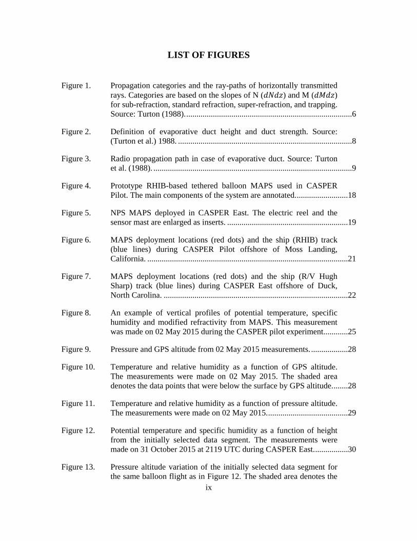
Figure 1. Propagation categories and the ray-paths of horizontally transmitted rays. Categories are based on the slopes of N (𝑑𝑑𝑑𝑑𝑑𝑑𝑑𝑑) and M (𝑑𝑑𝑑𝑑𝑑𝑑𝑑𝑑) for sub-refraction, standard refraction, super-refraction, and trapping. Source: Turton (1988). .................................................................................6
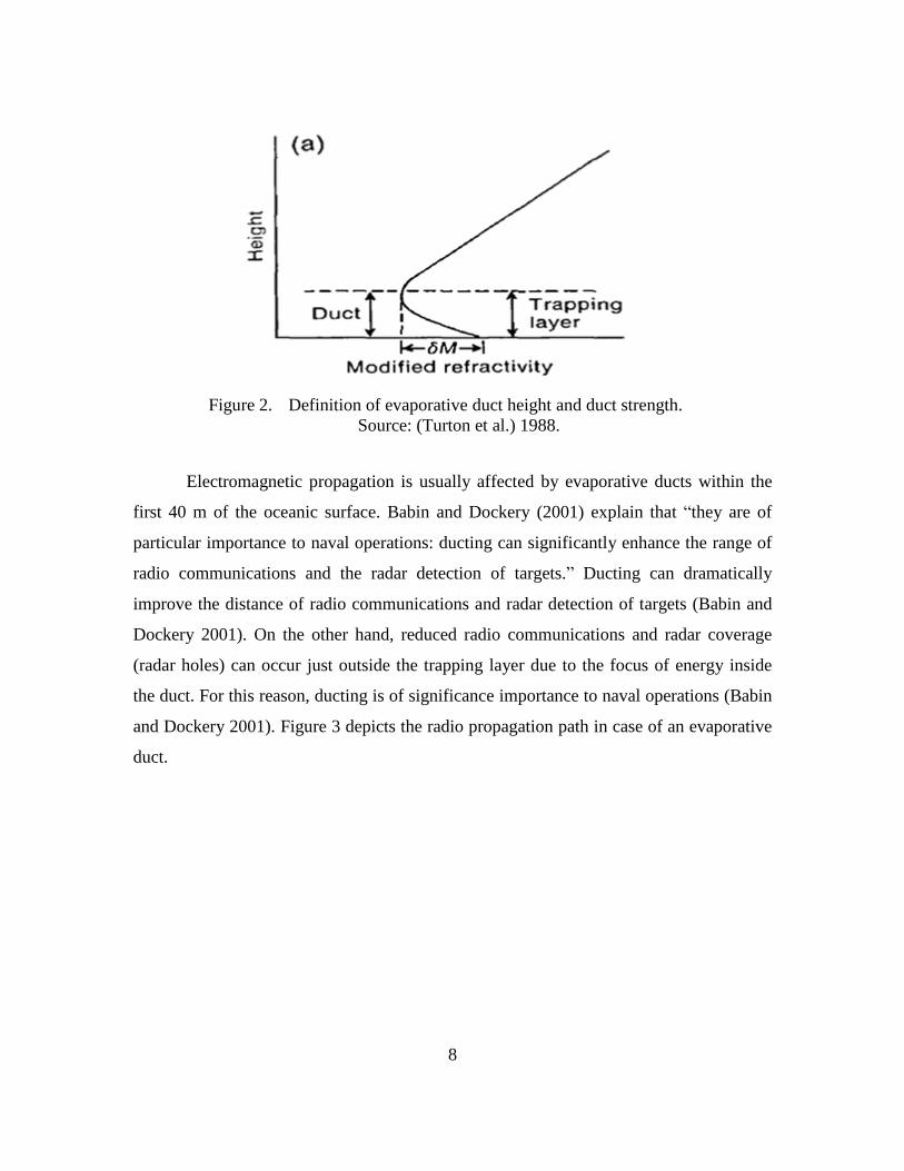
Figure 2. Definition of evaporative duct height and duct strength. Source: (Turton et al.) 1988. .....................................................................................8
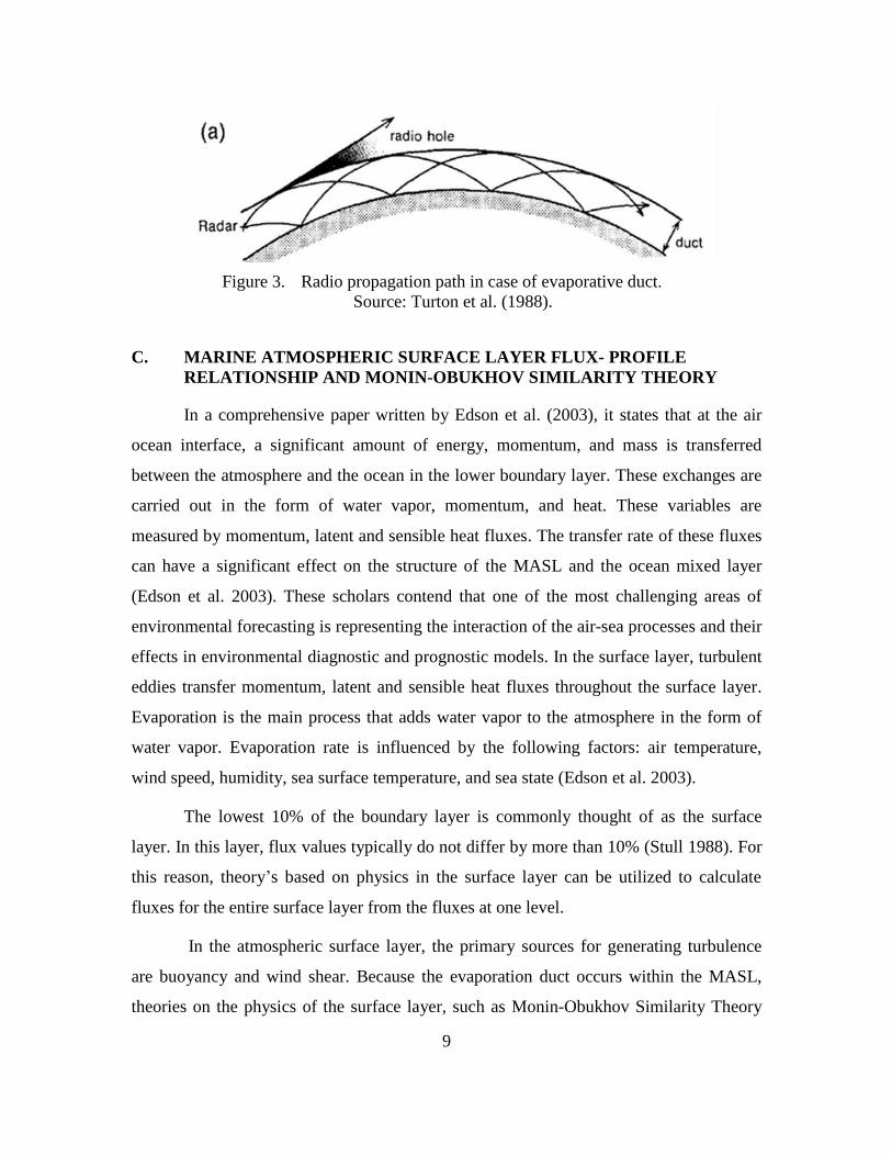
Figure 3. Radio propagation path in case of evaporative duct. Source: Turton et al. (1988). .................................................................................................9
Figure 4. Prototype RHIB-based tethered balloon MAPS used in CASPER Pilot. The main components of the system are annotated. .........................18
Figure 5. NPS MAPS deployed in CASPER East. The electric reel and the sensor mast are enlarged as inserts. ...........................................................19
Figure 6. MAPS deployment locations (red dots) and the ship (RHIB) track (blue lines) during CASPER Pilot offshore of Moss Landing, California. ..................................................................................................21
Figure 7. MAPS deployment locations (red dots) and the ship (R/V Hugh Sharp) track (blue lines) during CASPER East offshore of Duck, North Carolina. ..........................................................................................22
Figure 8. An example of vertical profiles of potential temperature, specific humidity and modified refractivity from MAPS. This measurement was made on 02 May 2015 during the CASPER pilot experiment............25
Figure 9. Pressure and GPS altitude from 02 May 2015 measurements. ..................28
Figure 10. Temperature and relative humidity as a function of GPS altitude. The measurements were made on 02 May 2015. The shaded area denotes the data points that were below the surface by GPS altitude. .......28
Figure 11. Temperature and relative humidity as a function of pressure altitude. The measurements were made on 02 May 2015. .......................................29
Figure 12. Potential temperature and specific humidity as a function of height from the initially selected data segment. The measurements were made on 31 October 2015 at 2119 UTC during CASPER East. ................30
Figure 13. Pressure altitude variation of the initially selected data segment for the same balloon flight as in Figure 12. The shaded area denotes the
x
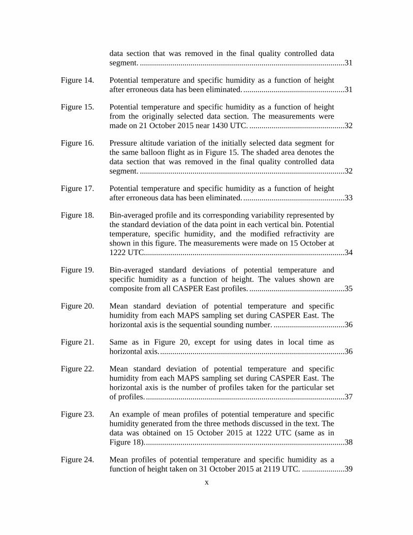
data section that was removed in the final quality controlled data segment. .....................................................................................................31
Figure 14. Potential temperature and specific humidity as a function of height after erroneous data has been eliminated. ..................................................31
Figure 15. Potential temperature and specific humidity as a function of height from the originally selected data section. The measurements were made on 21 October 2015 near 1430 UTC. ...............................................32
Figure 16. Pressure altitude variation of the initially selected data segment for the same balloon flight as in Figure 15. The shaded area denotes the data section that was removed in the final quality controlled data segment. .....................................................................................................32
Figure 17. Potential temperature and specific humidity as a function of height after erroneous data has been eliminated. ..................................................33
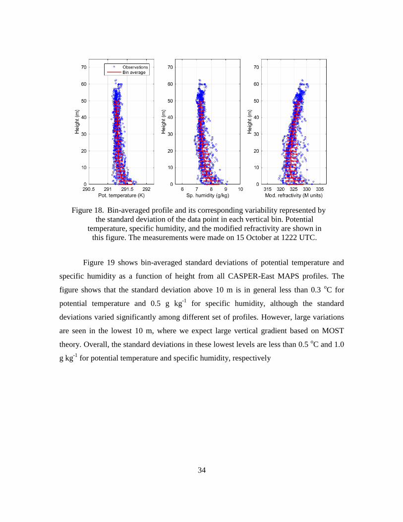
Figure 18. Bin-averaged profile and its corresponding variability represented by the standard deviation of the data point in each vertical bin. Potential temperature, specific humidity, and the modified refractivity are shown in this figure. The measurements were made on 15 October at 1222 UTC...................................................................................................34
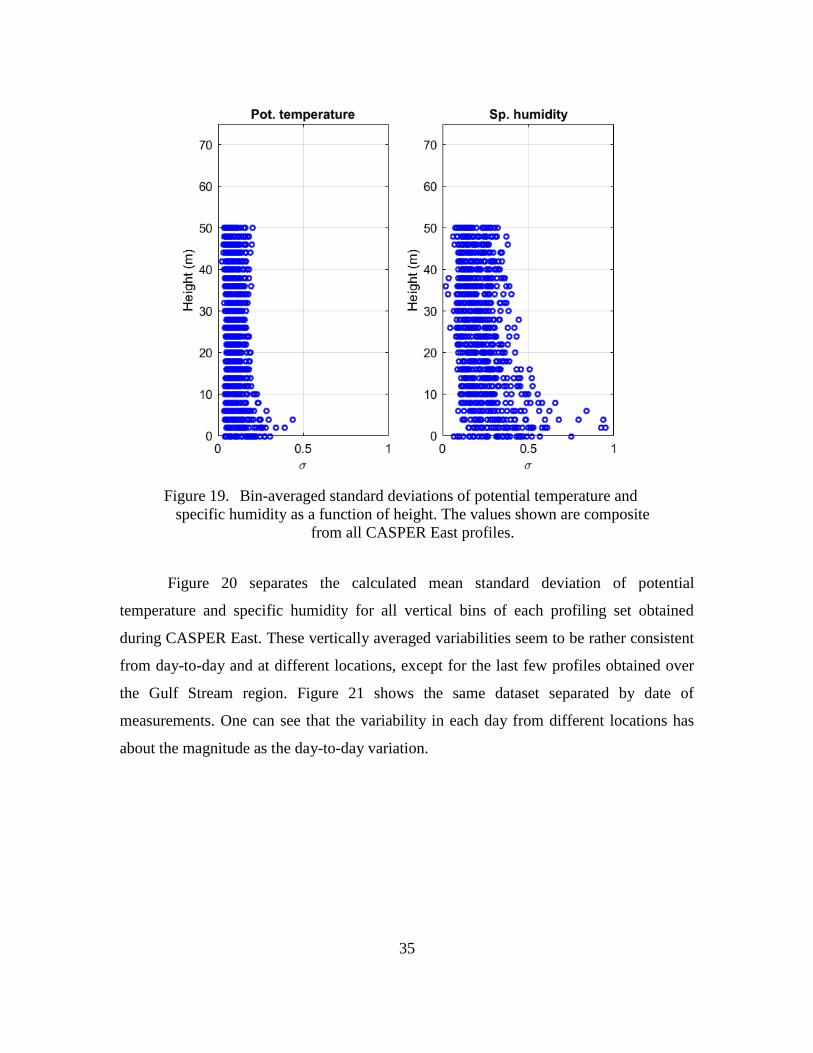
Figure 19. Bin-averaged standard deviations of potential temperature and specific humidity as a function of height. The values shown are composite from all CASPER East profiles. ...............................................35
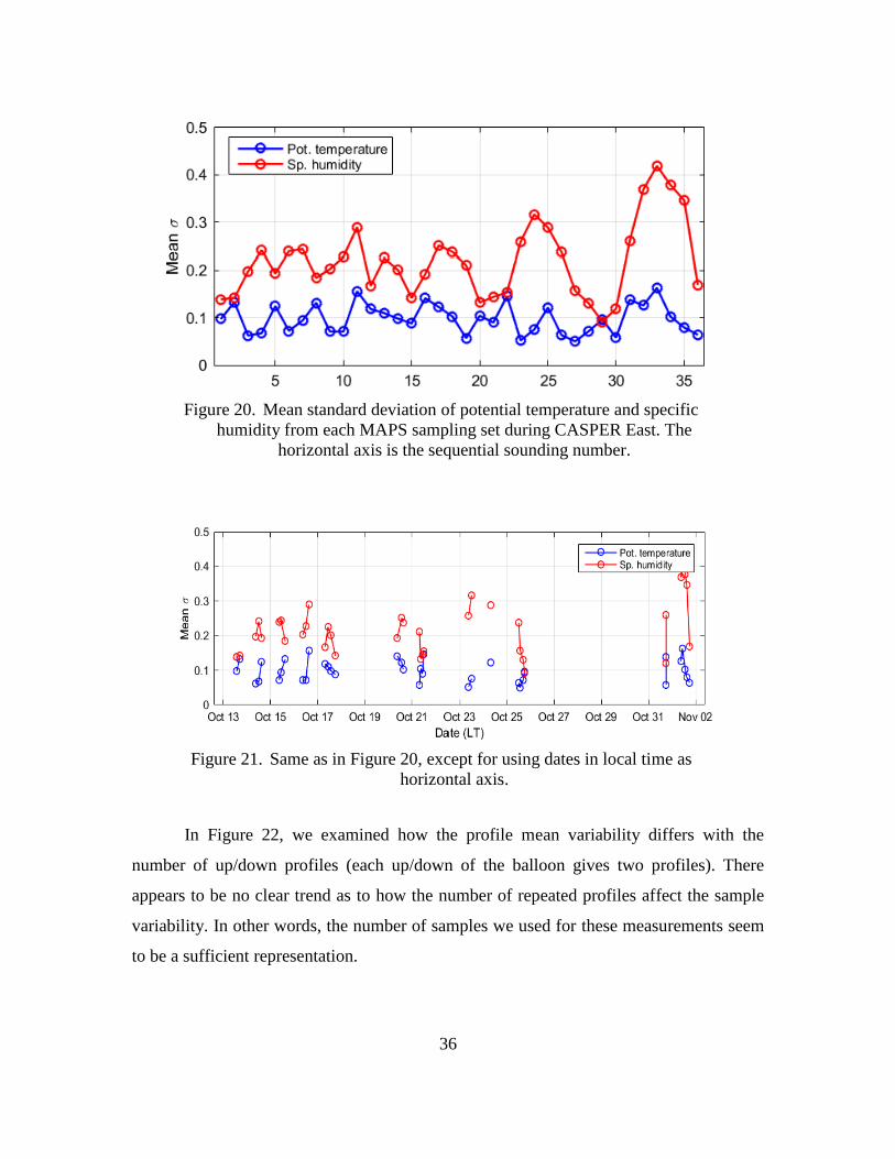
Figure 20. Mean standard deviation of potential temperature and specific humidity from each MAPS sampling set during CASPER East. The horizontal axis is the sequential sounding number. ...................................36
Figure 21. Same as in Figure 20, except for using dates in local time as horizontal axis. ...........................................................................................36
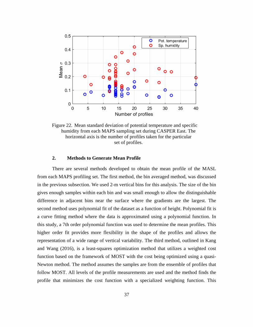
Figure 22. Mean standard deviation of potential temperature and specific humidity from each MAPS sampling set during CASPER East. The horizontal axis is the number of profiles taken for the particular set of profiles. ..................................................................................................37
Figure 23. An example of mean profiles of potential temperature and specific humidity generated from the three methods discussed in the text. The data was obtained on 15 October 2015 at 1222 UTC (same as in Figure 18). ..................................................................................................38
Figure 24. Mean profiles of potential temperature and specific humidity as a function of height taken on 31 October 2015 at 2119 UTC. .....................39
xi
Figure 25. Momentum (MF), latent heat (LHF) and sensible heat flux (SHF) during each CASPER East profiling period. ..............................................41
Figure 26. Mean profile of potential temperature, specific humidity and modified refractivity as a function of height for strongly stable case obtained on 13 October 2015 at 1947 UTC. ..............................................42
Figure 27. Mean profile of potential temperature, specific humidity and modified refractivity as a function of height for a case of stable stratification measured on 25 October 2015 at 1811 UTC. .......................43
Figure 28. Mean profile of potential temperature, specific humidity and modified refractivity as a function of height for a near neutral case. ........43
Figure 29. Mean profile of potential temperature, specific humidity and modified refractivity as a function of height for an unstable case. ............44
Figure 30. Mean profile of potential temperature, specific humidity and modified refractivity as a function of height for a strongly unstable case. ............................................................................................................44
Figure 31. Comparison of the measured and model evaporation duct properties for the entire CASPER-East profile set. ....................................................45
Figure 32. Observed or modeled evaporation duct properties as a function of ASTD. Input data to the model was obtained from R/V Sharp’s bow mast at 12 m, 1 m boat mast, and 12 m polynomial fit over static stability criteria for the entire CASPER-East profile set. ..........................45
Figure 33. Measured evaporative duct height verses estimated using COARE algorithm. ...................................................................................................46

xii
THIS PAGE INTENTIONALLY LEFT BLANK

xiii
LIST OF TABLES
Table 1. Comparison of the profiling components used in CASPER Pilot and
CASPER East.............................................................................................16
Table 2. Accuracy of all sensors of the NPS MAPS ................................................20
Table 3. CASPER Pilot NPS MAPS profiling data .................................................23
Table 4. PER-East NPS MAPS profiling data .........................................................24

xiv
THIS PAGE INTENTIONALLY LEFT BLANK
xv
LIST OF ACRONYMS AND ABBREVIATIONS
ABL atmospheric boundary layer
AREPS Advanced Refractive Effects Prediction System
ASTD air sea temperature difference
COAMPS Coupled Ocean/Atmosphere Mesoscale Prediction System
COARE Coupled Ocean-Atmosphere Response Experiment
EDH evaporation duct height
EDM evaporation duct model
EDS evaporation duct strength
EM electromagnetic
GPS Global Positioning System
IREPS Integrated Refractive Effects Prediction System
ISAR integrated infrared SST autonomous radiometer
MAPS Marine Atmospheric Profiling System
MASL maritime atmospheric surface layer
METOC meteorological and oceanographic
MOST Monin–Obukhov Similarity Theory
NAVSLaM Navy Atmospheric Vertical Surface Layer Model
NCOM Navy Coastal Ocean Model
NDBC National Data Buoy Center
NOAA National Oceanic and Atmospheric Administration
NPS Naval Postgraduate School
ONR Office of Naval Research
PJ Paulus-Jeske
RHIB rigid-hulled inflatable boat
R/V research vessel
SST sea surface temperature
TAWS Target Acquisition Weapons Software
TOGA COARE Tropical Ocean Global Atmosphere Coupled-Ocean Atmosphere
Response Experiment

xvi
THIS PAGE INTENTIONALLY LEFT BLANK
1
I. INTRODUCTION
A. THESIS OBJECTIVES
New insights and future developments in quantifying boundary layer refraction
profiles and therefore improving propagation predictions will heavily depend on
unraveling atmosphere-upper ocean processes on multiple scales using novel
measurement capabilities. To understand the evaporative duct, a direct measurement of
surface layer thermodynamic profile with high vertical resolution is needed. This has not
been done in previous field efforts. Unlike measurements on a tower or mast on land,
surface layer measurements over the sea are difficult to obtain at multiple levels. The
objective of this thesis will be to examine the feasibility of sampling the lowest few tens
of meters of marine atmospheric surface layer (MASL) in a minimally disturbed
environment. As part of the Coupled Air-Sea Processes and EM ducting Research
(CASPER) project, the Naval Postgraduate School (NPS) Meteorology Department has
developed a Marine Atmospheric Profiling System (MAPS) to sample the
thermodynamic profiles in the atmospheric surface layer. The dataset from this system
will fill the void of MASL profile measurements over the ocean. The system is designed
to make profiling measurements with multiple up/downs using an instrumented tethered
balloon to increase the number of samples at any given altitude to provide high statistical
significance. This thesis work will demonstrate the feasibility of the profiling system by
analyses of the data quality, methods of deriving MASL mean temperature and humidity
profiles from the raw measurements, and the derivation of evaporative duct properties
based on the measurements. Furthermore, the dataset will be used to evaluate evaporative
duct models such as Navy Atmospheric Vertical Surface Layer Model (NAVSLaM).
B. IMPORTANCE OF STUDY
Correctly quantifying the characteristics of the surface layer environment is
crucial to understanding low-altitude Electromagnetic (EM) propagation, particularly the
depiction of near-surface moisture and temperature profiles with high vertical resolution.
With the ultimate goal of improving evaporative duct prediction, we use a tethered
2
balloon based measurement system to obtain direct measurements of the surface layer
profiles. This collection of real-time near surface profile observations is essential for
evaporative duct model development and validation. EM propagation models also depend
on robust in situ profile measurements and/or highly accurate forecasts. Surface moisture
and temperature gradients affect the height of the evaporative duct that can act as a wave
guide for high frequencies (Edson et al. 1999). EM propagation is very sensitive to the
vertical variation in the atmospheric boundary layer (ABL) and would benefit from
improvements of model parameterizations with additional data for both research and
operational purposes. While near-surface data is key to improving surface flux
parameterization and understanding the mechanisms that couple the ocean and
atmosphere, it remains one of the greatest challenges to obtain the data observationally.
Ultimately, accurate prediction of the surface layer profiles and fluxes is the key to
weather prediction and EM prediction.
Bulk aerodynamic surface flux parameterization schemes are needed to explain
the exchanges of mass and energy across the air-sea interface, These are largely built
upon the Monin-Obukhov similarity theory (MOST) developed in 1954 (Liu et al. 1979).
Fairall et al. (1996b; 2003) further modified the bulk surface flux system by using data
obtained during the Tropical Ocean Global Atmosphere (TOGA) Coupled Ocean-
Atmosphere Response Experiment (COARE) that resulted in what is known as the
COARE bulk flux algorithm. COARE is now the most widely used flux algorithm in
most of the mesoscale and global scale forecast models. Limitations to the COARE
algorithm do exist, however, partly due to the inherent assumptions of MOST (e.g.,
Andreas et al. 2014). Thus, the need to collect high-quality data at the air-sea interface
continues in order to further improve surface flux parameterization algorithms and hence
forecast models.
C. NAVAL APPLICATION
Accurately characterizing the spatial and temporal variability of refractivity is
crucial to many important Navy and civilian applications. The ultimate goal of the project
is to enhance the Navy’s capability of predicting the performance of radar and
3
communications systems for tactical applications. With the removal of the rawinsonde
program from the U.S. Navy fleet in 2011, the accuracy of EM propagation prediction for
surface and airborne radar and communication operations depends primarily on the
modeled environmental forecasts that feed the propagation models. “EM propagation is
sensitive to even slight changes in the ABL temperature and moisture gradients” (Babin
1997). Near surface measurements are critical to determining and accurately forecasting
these gradients and the structure of the ABL. Advanced Refractive Effects Prediction
System (AREPS) and Target Acquisition Weapons Software (TAWS), in particular,
require accurate ABL profile inputs to effectively predict EM propagation, radar ranges,
and weapon sensor effectiveness.
The Navy is committed to achieving superiority of the electromagnetic spectrum
(EMS). The 2015 Electromagnetic Maneuver Warfare (EMW) Campaign Plan “is the
Navy’s warfighting approach to gain decisive military advantage in the EMS to enable
freedom of action across all Navy mission areas.” Commander Navy Meteorology and
Oceanography Command, Rear Admiral Gallaudet has outlined a strategy to advance
Navy’s electromagnetic warfare capabilities in a recent article. One of the goals of this
strategy is to improve Naval Oceanography’s Environmental and Prediction Capabilities
by advancing our environmental sensing capabilities:
The need for additional sensing is most critical in the lowest portion of the
atmosphere where the evaporative duct forms and impacts the propagation
of signals. We will develop, evaluate and transition autonomous/
unmanned platforms and sensors that enable persistent, physical
battlespace awareness, potentially through a new Littoral Battlespace
increment. We will improve the vertical resolution of our observations in
the lowest portion of the atmosphere where impacts on EMW propagation
is the highest. (Gallaudet 2016)

4
THIS PAGE INTENTIONALLY LEFT BLANK
5
II. BACKGROUND
A. ATMOSPHERIC REFRACTION
“Atmospheric refractive conditions can significantly affect the performance of
shipboard radars and communications at sea and near shore” (Battan 1973).
Characterizing the spatial and temporal variability of refractivity is thus crucial to many
important Navy and civilian applications. When electromagnetic radiation travels through
the atmosphere, they follow curved instead of straight paths such as in the outer space
without the atmosphere. The bending of radio waves is usually quantified by the index of
refraction defined as the ratio between the speed of light in a vacuum over that in a
medium. The index of refraction is affected by temperature, pressure and humidity, the
latter being the most important, as described in Equation (1) (Bean and Dutton 1968):
𝑁 = (𝑛 − 1) × 106 = 76.7
𝑇(𝑝 +
4810𝑒
𝑇) (1)
where N is refractivity, n is the index of refraction, T is the atmospheric temperature (K),
p is the total atmospheric pressure (hPa), and e is the water vapor pressure (hPa). To
consider propagation over the earth with a curvature, a modified refraction, M, is defined
so that one can considered the earth as a hypothetically flat surface:
𝑀 = 𝑁 +𝑧
10−6𝑟𝑒(𝑛 − 1) × 106 = 𝑁 + 0.157𝑧 (2)
where re is the earth’s radius in meters and z is altitude in meters (Bean and Dutton
1968).
The refractivity profile in the atmosphere determines the curvature of the ray
depends on the rate of change of the refractive index with height.
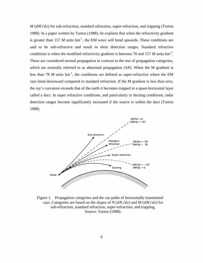
Figure 1 illustrates the refractivity propagation categories and the ray-paths of
horizontally transmitted rays. These categories are based on the slopes of N (𝑑𝑁 𝑑𝑧⁄ ) or
6
M (𝑑𝑀 𝑑𝑧⁄ ) for sub-refraction, standard refraction, super-refraction, and trapping (Turton
1988). In a paper written by Turton (1988), he explains that when the refractivity gradient
is greater than 157 M units km-1
, the EM wave will bend upwards. These conditions are
said to be sub-refractive and result in short detection ranges. Standard refractive
conditions is when the modified refractivity gradient is between 78 and 157 M units km-1
.
These are considered normal propagation in contrast to the rest of propagation categories,
which are normally referred to as abnormal propagation (AP). When the M gradient is
less than 78 M units km-1
, the conditions are defined as super-refractive where the EM
rays bend downward compared to standard refraction. If the M gradient is less than zero,
the ray’s curvature exceeds that of the earth it becomes trapped in a quasi-horizontal layer
called a duct. In super refractive conditions, and particularly in ducting conditions, radar
detection ranges become significantly increased if the source is within the duct (Turton
1988).
Figure 1. Propagation categories and the ray-paths of horizontally transmitted
rays. Categories are based on the slopes of N (𝑑𝑁 𝑑𝑧⁄ ) and M (𝑑𝑀 𝑑𝑧⁄ ) for
sub-refraction, standard refraction, super-refraction, and trapping.
Source: Turton (1988).
7
B. EVAPORATIVE DUCT
Evaporation ducts are ever present over the ocean, and are associated with strong
vertical water vapor gradients near the sea surface (Babin et al. 1997). This type of duct
occurs in the MASL as a result of sea surface evaporation and this evaporation is enough
to cause the bending of electro-magnetic radiation so that it becomes trapped in this area
(i.e., ducting) (Babin et al. 1997). The evaporation duct is hence a special type of surface
duct with the trapping layer extending to the surface. In identifying the trapping layers of
the troposphere, the modified refractivity expressed in Equation (2) is most often used to
characterize the evaporation duct properties. Traditionally, according to a paper written
by Babin and Dockery (2001), “the evaporation duct has been characterized by
determining only the height of the duct as defined by the altitude at which 𝑑𝑀 𝑑𝑧 = 0⁄ .
However, it is the slope 𝑑𝑀 𝑑𝑧⁄ that is used in propagation models, and a given duct
height may result from a variety of different shapes of M profiles. As Equation (1) and
(2) indicate, these M-profile curvatures are primarily affected by vertical temperature and
moisture profiles and hence by atmospheric static stability.” Gehman points out in a
paper written in 2000, “the actual slope is more important in uniquely determining
electromagnetic propagation effects than the duct height alone.” Duct strength can be
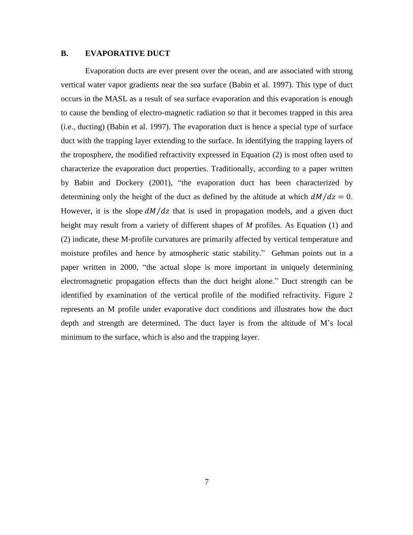
identified by examination of the vertical profile of the modified refractivity. Figure 2
represents an M profile under evaporative duct conditions and illustrates how the duct
depth and strength are determined. The duct layer is from the altitude of M’s local
minimum to the surface, which is also and the trapping layer.
8
Figure 2. Definition of evaporative duct height and duct strength.
Source: (Turton et al.) 1988.
Electromagnetic propagation is usually affected by evaporative ducts within the
first 40 m of the oceanic surface. Babin and Dockery (2001) explain that “they are of
particular importance to naval operations: ducting can significantly enhance the range of
radio communications and the radar detection of targets.” Ducting can dramatically
improve the distance of radio communications and radar detection of targets (Babin and
Dockery 2001). On the other hand, reduced radio communications and radar coverage
(radar holes) can occur just outside the trapping layer due to the focus of energy inside
the duct. For this reason, ducting is of significance importance to naval operations (Babin
and Dockery 2001). Figure 3 depicts the radio propagation path in case of an evaporative
duct.
9
Figure 3. Radio propagation path in case of evaporative duct. Source: Turton et al. (1988).
C. MARINE ATMOSPHERIC SURFACE LAYER FLUX- PROFILE
RELATIONSHIP AND MONIN-OBUKHOV SIMILARITY THEORY
In a comprehensive paper written by Edson et al. (2003), it states that at the air
ocean interface, a significant amount of energy, momentum, and mass is transferred
between the atmosphere and the ocean in the lower boundary layer. These exchanges are
carried out in the form of water vapor, momentum, and heat. These variables are
measured by momentum, latent and sensible heat fluxes. The transfer rate of these fluxes
can have a significant effect on the structure of the MASL and the ocean mixed layer
(Edson et al. 2003). These scholars contend that one of the most challenging areas of
environmental forecasting is representing the interaction of the air-sea processes and their
effects in environmental diagnostic and prognostic models. In the surface layer, turbulent
eddies transfer momentum, latent and sensible heat fluxes throughout the surface layer.
Evaporation is the main process that adds water vapor to the atmosphere in the form of
water vapor. Evaporation rate is influenced by the following factors: air temperature,
wind speed, humidity, sea surface temperature, and sea state (Edson et al. 2003).
The lowest 10% of the boundary layer is commonly thought of as the surface
layer. In this layer, flux values typically do not differ by more than 10% (Stull 1988). For
this reason, theory’s based on physics in the surface layer can be utilized to calculate
fluxes for the entire surface layer from the fluxes at one level.
In the atmospheric surface layer, the primary sources for generating turbulence
are buoyancy and wind shear. Because the evaporation duct occurs within the MASL,
theories on the physics of the surface layer, such as Monin-Obukhov Similarity Theory
10
(MOST) are used for evaporative duct modeling. MOST is based on scaling analysis to
derive the relationship between the mean wind, temperature, and specific humidity
profiles to surface layer turbulent fluxes (Edson et al. 2003). The resultant non-
dimensional gradients can be expressed as:
𝜅𝑧
𝑢∗
𝜕𝑢
𝜕𝑧= 𝜑𝑚 (
𝑧
𝐿) (3)
𝜅𝑧
𝜃∗
𝜕�̅�
𝜕𝑧= 𝜑ℎ (
𝑧
𝐿) (4)
𝜅𝑧
𝑞∗
𝜕�̅�
𝜕𝑧= 𝜑ℎ (
𝑧
𝐿) (5)
where von Karman’s constant 𝜅 ≈ 0.35 − 0.40 derived from measurements, L is the
Monin-Obukhov length: 𝐿 =𝑢∗
3
𝜅𝑔𝑤′𝛳′̅̅ ̅̅ ̅̅ ̅ , g is gravity, z is height, and 𝜑𝑚 (
𝑧
𝐿) and 𝜑𝑚 (
𝑧
𝐿) are
non-dimensional U functions that account for the effects of thermal stability of the
surface layer. In addition, 𝑢∗ is the frictional velocity, 𝑞∗ is specific humidity scale and 𝜃∗
is the temperature scale. According to Edson, these are considered the scaling parameters
of the surface layers. The left hand side of the equations represents the non-dimensional
vertical gradient of mean wind, mean potential temperature, and mean specific humidity.
The right hand side of the equations shows that these mean gradients are functions of
height non-dimensionalized by L, signifying the effects of thermal stability. These
universal functions have been empirically derived from measurements in the field.
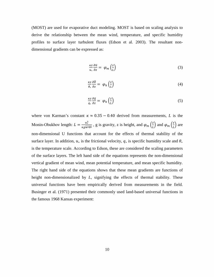
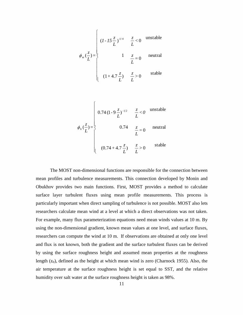
Businger et al. (1971) presented their commonly used land-based universal functions in
the famous 1968 Kansas experiment:
11
stable0 > ) 4.7 + (0.74
neutral0 =
0.74
unstable)91(74.0
)(
21
L
z
L
z
L
z
0 < L
z
L
z -
= L
z
h
The MOST non-dimensional functions are responsible for the connection between
mean profiles and turbulence measurements. This connection developed by Monin and
Obukhov provides two main functions. First, MOST provides a method to calculate
surface layer turbulent fluxes using mean profile measurements. This process is
particularly important when direct sampling of turbulence is not possible. MOST also lets
researchers calculate mean wind at a level at which a direct observations was not taken.
For example, many flux parameterization equations need mean winds values at 10 m. By
using the non-dimensional gradient, known mean values at one level, and surface fluxes,
researchers can compute the wind at 10 m. If observations are obtained at only one level
and flux is not known, both the gradient and the surface turbulent fluxes can be derived
by using the surface roughness height and assumed mean properties at the roughness
length (z0), defined as the height at which mean wind is zero (Charnock 1955). Also, the
air temperature at the surface roughness height is set equal to SST, and the relative
humidity over salt water at the surface roughness height is taken as 98%.
stable0 > ) 4.7 + (1
neutral0 =
1
unstable0)(
)(
4/1
L
z
L
z
L
z
< L
z
L
z15 - 1
= L
z
-
m
12
The stability function in MOST was developed from measurements over land,
which brings into question its validity over the ocean. The fluid interface over the ocean
whose roughness changes with the wind generated wave and swells from distant storms
makes the MASL much more complicated than its counterpart over land. Additionally,
MOST assumes horizontally homogenous conditions. It was found (Tellado 2013) that
significant inhomogeneity always exists over the coastal ocean near Monterey Bay. The
homogenous assumption thus may not hold true near the coast or close to a frontal
boundary.
D. EVAPORATIVE DUCT MODELS
According to paper written by Babin (1997), “The general approach for all
evaporation duct models (EDM) involves finding an expression for the vertical
refractivity gradient in terms of atmospheric variables.” Since the evaporative duct
occurs in the surface layer, MOST is typically used to derive the mean vertical profile.
EDM’s calculate the modified refractivity gradient, from this, evaporative duct properties
such as duct strength and height can be obtained by evaluating the profile (Cherrett
2015). A comprehensive summary of this approach is provided in Babin (1997). There
are currently two types of evaporation duct models: the potential refractivity model and
the LKB-based models.
From 1978 until 2012, the Paulus-Jeske (PJ) evaporation duct model (Jeske 1973;
Paulus 1984, 1985, 1989) was the U.S. Navy’s most widely used evaporation duct model
(Babin 1997). It was incorporated into Integrated Refractive Effects Prediction System
(IREPS) and then AREPS Tactical Decision Aids (TDA). The PJ model uses the potential
refractivity quantity, which calculates refractivity index using “potential temperature,
potential water vapor pressure, and 1000 hPa atmospheric pressure as opposed to air
temperature, water vapor pressure, and surface pressure” (Jeske 1973). PJ model allocates
values of wind speed, relative humidity, and air temperature to a height of 6 m, regardless
“of the actual observation height. SST is also used and surface pressure is assigned a
constant value of 1000 hPa” (Paulus 1984). An additional parameter distinctive to the PJ
model is that instead of using the typical -0.157 critical gradient for potential refractivity
13
it uses a critical potential refractivity gradient of -0.125 to determine ducting (Babin
1997). Cook and Burk (1992) indicated certain inadequacy of the PJ model. They
revealed that “when properly non-dimensionalized the vertical gradient of potential
refractivity was not a single universal function of z/L and that potential refractivity in
stable conditions did not obey MOST” (Babin 1997). This implied that for stable
conditions, the principle theory for this model in using potential refractivity was
inappropriate.
Liu et al. (1979) developed a marine atmospheric surface layer model that is
referred to as Liu, Katsaros, and Businger (LKB) and used it for deriving air–sea
exchanges of heat, moisture, and momentum. The LKB model included the interfacial
molecular effects at the sea surface and matched the mean wind and scalar profiles from
the MOST theory with those in the molecular sublayer. Their approach was used to
represent surface layer turbulence fluxes, which leads to the MOST-based surface flux
parameterizations. The Tropical Ocean and Global Atmosphere Coupled Ocean–
Atmosphere Response Experiment (TOGA COARE) (Fairall et al. 1996) project later
refined the LKB MASL models by incorporating the results of more than 10,000 hours of
atmospheric and oceanic measurements from buoys, ships and aircraft. Their efforts led
to the COARE surface flux algorithm that is currently the most widely used surface flux
parameterization scheme extensively used in various mesoscale and global scale models
(Fairall et al. 1996, 2003).
There are several LKB-based evaporation duct models; the most significant
difference among them is the use of different stability function,𝜓(𝑧 𝐿⁄ ) to “account for
deviations from neutral stability in the atmospheric surface layer and are integrated forms
of the dimensionless gradient functions” (Blackadar 1993). The most notable LKB-based
model is the Naval Postgraduate School (NPS) evaporation duct model described in
Frederickson et al. (2000). In 2012, The NPS model was developed and integrated into
AREPS and is now called the NAVSLaM (Navy Atmospheric Vertical Surface Layer
Model).
14
E. COUPLED AIR-SEA PROCESSES AND ELECTROMAGNETIC
DUCTING RESEARCH
The Coupled Air-Sea Processes and EM ducting Research (CASPER), is
sponsored by the Office of Navy Research (ONR) 2014 Multi-disciplinary University
Research Initiative (MURI) to address overarching knowledge gaps related to
electromagnetic wave propagation in coastal MABL. The objective of CASPER is to
fully characterize the MABL as an EM propagation environment. There are three
components to the CASPER project: theoretical developments, field program, and
numerical modeling efforts. This thesis is centered on the field program that focuses on
employing new environmental measurement techniques and novel sampling strategies to
obtain a comprehensive and cohesive dataset to address air-sea interaction processes that
affect EM propagation and for extensive model evaluation and testing and new
measurement capabilities. “The field components have two main campaigns: CASPER-
East (Duck, NC) and CASPER-West (Southern California). With these two operations,
CASPER plans to fully characterize the marine atmospheric boundary layer (MABL) as
an electromagnetic (EM) propagation environment. The emphasis will be on spatial and
temporal heterogeneities and surface wave/swell effects” (Wang et al.).
Prior to onset of Casper East, the CASPER pilot experiment was conducted
offshore and at the shoreline of Moss Landing, CA. to test out a few of the key platforms
and sensors. CASPER pilot took place from April 20, 2015 to May 2, 2015, with
CASPER-East being conducted off the coast of Duck, North Carolina from October 10,
to November 6, 2015. All data used in this study were collected during CASPER Pilot
and CASPER East.
15
III. NPS MASL PROFILING SYSTEM
A. SYSTEM AND SENSOR INFORMATION
We have developed a profiling system to sample the MASL in an undisturbed
environment. The NPS Marine Atmospheric Surface Layer Profiling system (NPS
MAPS) includes two components: the profiling and ship mast components. The profiling
component intends to sample the variation of temperature and relative humidity with
height (T/RH profiles) with multiple ascends and descends of the probes, while the ship
mast component provide auxiliary data collected continuously at a fixed level. The
auxiliary data includes wind speed and direction, pressure, GPS position, and sea surface
temperature (SST). Temperature and dew point temperature are also measured from the
mast. The data from both components are used to derive refractivity profiles used to
identify the characteristics of evaporation duct and to make diagnostic model calculations
of the evaporation duct.
A prototype of the profiling system was tested in CASPER pilot experiment in
April/May of 2015. An improved system was used in CASPER East field campaign. In
the following description, both the prototype system and the improved system will be
described.
1. The Profiling Component
The profiling component is mainly composed of a radiosonde, a tethered balloon,
and a radiosonde receiver/display system. It also includes a reel that controls the up and
down movement of the tethered balloon. The radiosonde is the iMet-1-ABX sonde that
measures temperature, relative humidity, pressure, GPS time and locations. Since a
normal rawinsonde on a free flying balloon obtains wind from the time and position of
the sonde, the tethered sonde cannot provide wind measurements. In Table 1 below,
different specifications of the profiling component are compared between the CASPER
pilot and CASPER East deployments. CASPER East represents significant improvements
from the prototype in CASPER pilot. The real-time transmission and display of the
profile is a major improvement because problematic probes or some sampling issues can

16
be identified and corrected on the spot to ensure measurement success. The use of the
electric reel made it possible for multiple ascends/descends without extreme fatigue of
the operator, especially in windy conditions. Using a smaller sized balloon and thinner
tetherline also helped to reduce the excess pulling of the balloon.
Table 1. Comparison of the profiling components used in CASPER Pilot and
CASPER East.
Specifications CASPER Pilot CASPER East
Sonde
iMet-1-ABX
modified to record
data on microchips
iMet-1-ABX
Data collection Self-recording
Transmitted and
received in real-
time using radio
receiver
Data display None Real-time display
on tablet
Sonde attachment
Separately tethered
free dangling ~5 m
below the balloon
Attached directly
to the tetherline of
the balloon ~3 m
below the balloon
Balloon 3.3 m3 Helikite 2.0 m
3 Helikite
Balloon motion control manual Electric fishing reel
Power need None Marine battery to
power fishing reel
In both CASPER pilot and East, we used the Helikite as the tethered lifting
system. The Helikite aerostats are kite-balloon hybrid aerostat. In low wind conditions,
the lift is mainly from the lighter-than-air balloon, while in wind conditions, the kite
produces significant lift. The major advantage of the Helikite is its stability compared to
normal tethered balloons and kites, especially near the surface where there is significant
turbulence. In conditions with some wind, the Helikites fly at about 45o angle. The 2 m
2
Helikite used in CASPER East is 9 ft × 7 ft in size (length × width) and provides 0.8 kg
of lift in no wind conditions and ~4 kg of lift in wind speed of ~6.7 ms-1
(15 mph). When
fully deployed, the radiosonde flies about 50 m above the waterline and when fully reeled
in the radiosonde lies below 1 m from the ocean surface.
17
2. Sensors on Mast
The small mast on the ship hosts a suite of sensors that provide auxiliary data for
ED property retrieval and/or EM model input. These sensors include a gyro stabilized
electronic compass which provides accurate heading, pitch, and roll in various dynamic
conditions, a Vaisala Weather Transmitter WXT520 that measures barometric pressure,
humidity, temperature, wind speed and direction. Sea surface temperature was measured
by a thermistor located about 0.02 m below the sea surface. The sensors and the data
acquisition system were all powered by a 12V marine battery.
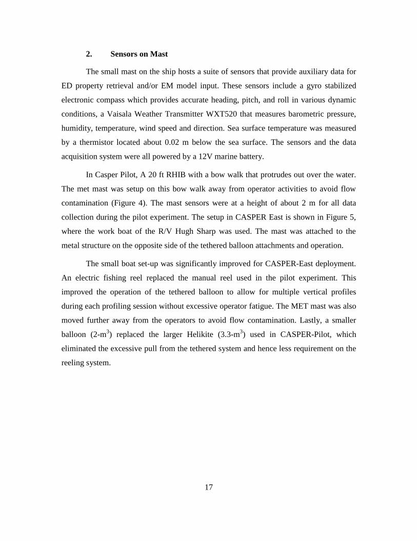
In Casper Pilot, A 20 ft RHIB with a bow walk that protrudes out over the water.
The met mast was setup on this bow walk away from operator activities to avoid flow
contamination (Figure 4). The mast sensors were at a height of about 2 m for all data
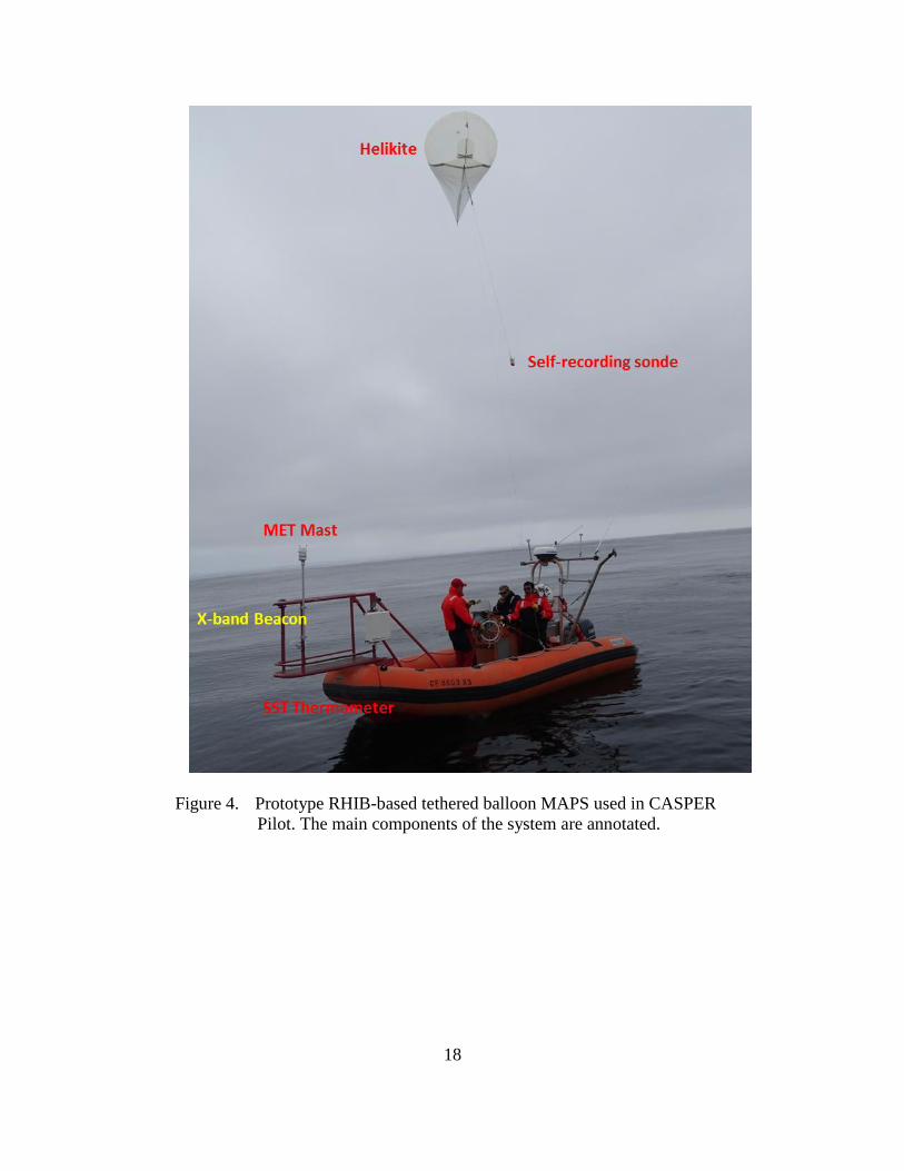
collection during the pilot experiment. The setup in CASPER East is shown in Figure 5,
where the work boat of the R/V Hugh Sharp was used. The mast was attached to the
metal structure on the opposite side of the tethered balloon attachments and operation.
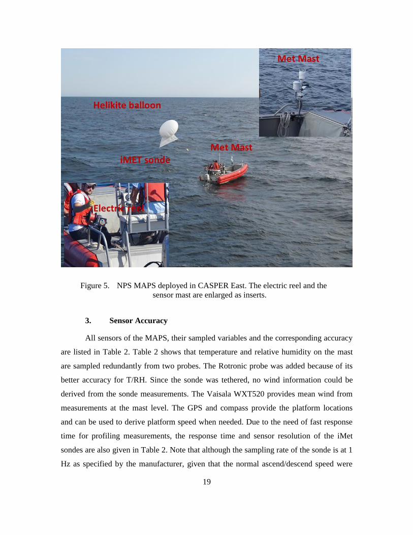
The small boat set-up was significantly improved for CASPER-East deployment.
An electric fishing reel replaced the manual reel used in the pilot experiment. This
improved the operation of the tethered balloon to allow for multiple vertical profiles
during each profiling session without excessive operator fatigue. The MET mast was also
moved further away from the operators to avoid flow contamination. Lastly, a smaller
balloon (2-m3) replaced the larger Helikite (3.3-m
3) used in CASPER-Pilot, which
eliminated the excessive pull from the tethered system and hence less requirement on the
reeling system.
18
Figure 4. Prototype RHIB-based tethered balloon MAPS used in CASPER
Pilot. The main components of the system are annotated.
19
Figure 5. NPS MAPS deployed in CASPER East. The electric reel and the
sensor mast are enlarged as inserts.
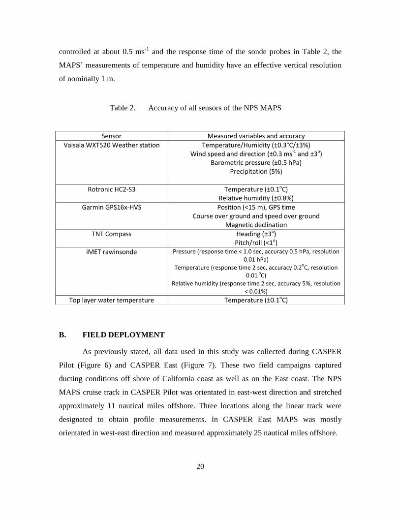
3. Sensor Accuracy
All sensors of the MAPS, their sampled variables and the corresponding accuracy
are listed in Table 2. Table 2 shows that temperature and relative humidity on the mast
are sampled redundantly from two probes. The Rotronic probe was added because of its
better accuracy for T/RH. Since the sonde was tethered, no wind information could be
derived from the sonde measurements. The Vaisala WXT520 provides mean wind from
measurements at the mast level. The GPS and compass provide the platform locations
and can be used to derive platform speed when needed. Due to the need of fast response
time for profiling measurements, the response time and sensor resolution of the iMet
sondes are also given in Table 2. Note that although the sampling rate of the sonde is at 1
Hz as specified by the manufacturer, given that the normal ascend/descend speed were
20
controlled at about 0.5 ms-1
and the response time of the sonde probes in Table 2, the
MAPS’ measurements of temperature and humidity have an effective vertical resolution
of nominally 1 m.
Table 2. Accuracy of all sensors of the NPS MAPS
B. FIELD DEPLOYMENT
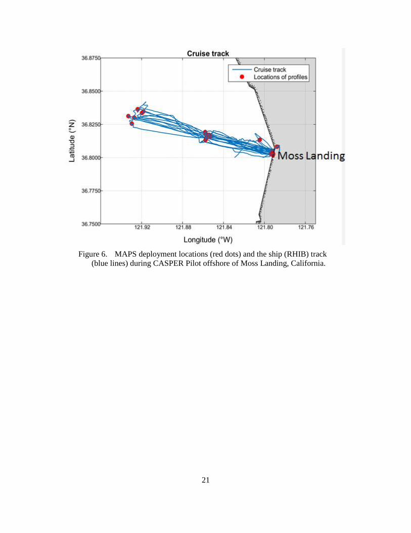
As previously stated, all data used in this study was collected during CASPER
Pilot (Figure 6) and CASPER East (Figure 7). These two field campaigns captured
ducting conditions off shore of California coast as well as on the East coast. The NPS
MAPS cruise track in CASPER Pilot was orientated in east-west direction and stretched
approximately 11 nautical miles offshore. Three locations along the linear track were
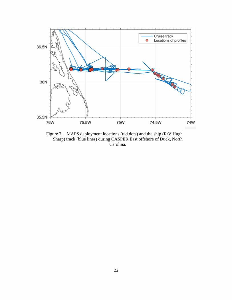
designated to obtain profile measurements. In CASPER East MAPS was mostly
orientated in west-east direction and measured approximately 25 nautical miles offshore.
Sensor Measured variables and accuracy
Vaisala WXT520 Weather station Temperature/Humidity (±0.3°C/±3%) Wind speed and direction (±0.3 ms-1 and ±3o)
Barometric pressure (±0.5 hPa) Precipitation (5%)
Rotronic HC2-S3 Temperature (±0.1oC) Relative humidity (±0.8%)
Garmin GPS16x-HVS Position (<15 m), GPS time Course over ground and speed over ground
Magnetic declination
TNT Compass Heading (±3o) Pitch/roll (<1o)
iMET rawinsonde Pressure (response time < 1.0 sec, accuracy 0.5 hPa, resolution 0.01 hPa)
Temperature (response time 2 sec, accuracy 0.2oC, resolution
0.01 o
C) Relative humidity (response time 2 sec, accuracy 5%, resolution
< 0.01%)
Top layer water temperature Temperature (±0.1oC)
21
Figure 6. MAPS deployment locations (red dots) and the ship (RHIB) track
(blue lines) during CASPER Pilot offshore of Moss Landing, California.
22
Figure 7. MAPS deployment locations (red dots) and the ship (R/V Hugh
Sharp) track (blue lines) during CASPER East offshore of Duck, North
Carolina.
23
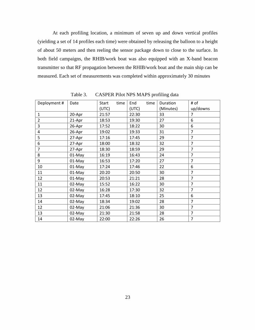
At each profiling location, a minimum of seven up and down vertical profiles
(yielding a set of 14 profiles each time) were obtained by releasing the balloon to a height
of about 50 meters and then reeling the sensor package down to close to the surface. In
both field campaigns, the RHIB/work boat was also equipped with an X-band beacon
transmitter so that RF propagation between the RHIB/work boat and the main ship can be
measured. Each set of measurements was completed within approximately 30 minutes
Table 3. CASPER Pilot NPS MAPS profiling data
Deployment # Date Start time (UTC)
End time (UTC)
Duration (Minutes)
# of up/downs
1 20-Apr 21:57 22:30 33 7
2 21-Apr 18:53 19:30 27 6
3 26-Apr 17:52 18:22 30 6
4 26-Apr 19:02 19:33 31 7
5 27-Apr 17:16 17:45 29 7
6 27-Apr 18:00 18:32 32 7
7 27-Apr 18:30 18:59 29 7
8 01-May 16:19 16:43 24 7
9 01-May 16:53 17:20 27 7
10 01-May 17:24 17:46 22 6
11 01-May 20:20 20:50 30 7
12 01-May 20:53 21:21 28 7
11 02-May 15:52 16:22 30 7
12 02-May 16:28 17:30 32 7
13 02-May 17:45 18:10 25 6
14 02-May 18:34 19:02 28 7
12 02-May 21:06 21:36 30 7
13 02-May 21:30 21:58 28 7
14 02-May 22:00 22:26 26 7
24
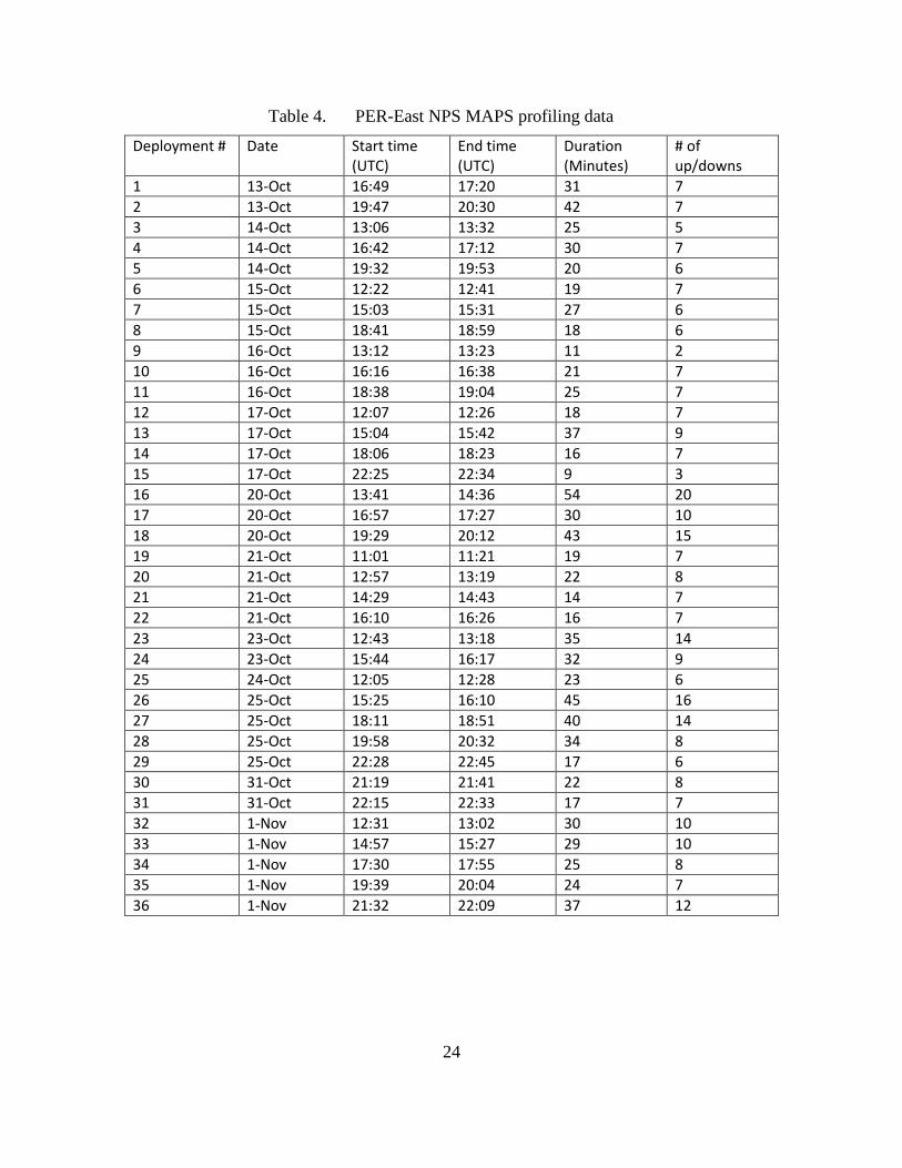
Table 4. PER-East NPS MAPS profiling data
Deployment # Date Start time (UTC)
End time (UTC)
Duration (Minutes)
# of up/downs
1 13-Oct 16:49 17:20 31 7
2 13-Oct 19:47 20:30 42 7
3 14-Oct 13:06 13:32 25 5
4 14-Oct 16:42 17:12 30 7
5 14-Oct 19:32 19:53 20 6
6 15-Oct 12:22 12:41 19 7
7 15-Oct 15:03 15:31 27 6
8 15-Oct 18:41 18:59 18 6
9 16-Oct 13:12 13:23 11 2
10 16-Oct 16:16 16:38 21 7
11 16-Oct 18:38 19:04 25 7
12 17-Oct 12:07 12:26 18 7
13 17-Oct 15:04 15:42 37 9
14 17-Oct 18:06 18:23 16 7
15 17-Oct 22:25 22:34 9 3
16 20-Oct 13:41 14:36 54 20
17 20-Oct 16:57 17:27 30 10
18 20-Oct 19:29 20:12 43 15
19 21-Oct 11:01 11:21 19 7
20 21-Oct 12:57 13:19 22 8
21 21-Oct 14:29 14:43 14 7
22 21-Oct 16:10 16:26 16 7
23 23-Oct 12:43 13:18 35 14
24 23-Oct 15:44 16:17 32 9
25 24-Oct 12:05 12:28 23 6
26 25-Oct 15:25 16:10 45 16
27 25-Oct 18:11 18:51 40 14
28 25-Oct 19:58 20:32 34 8
29 25-Oct 22:28 22:45 17 6
30 31-Oct 21:19 21:41 22 8
31 31-Oct 22:15 22:33 17 7
32 1-Nov 12:31 13:02 30 10
33 1-Nov 14:57 15:27 29 10
34 1-Nov 17:30 17:55 25 8
35 1-Nov 19:39 20:04 24 7
36 1-Nov 21:32 22:09 37 12
25
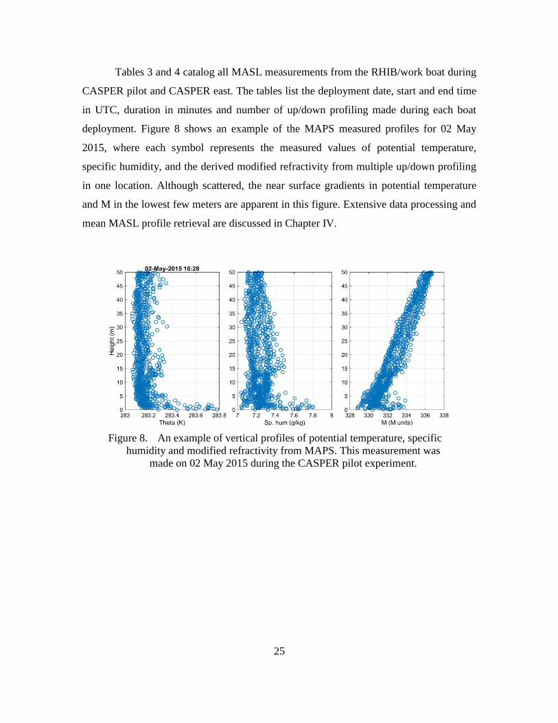
Tables 3 and 4 catalog all MASL measurements from the RHIB/work boat during
CASPER pilot and CASPER east. The tables list the deployment date, start and end time
in UTC, duration in minutes and number of up/down profiling made during each boat
deployment. Figure 8 shows an example of the MAPS measured profiles for 02 May
2015, where each symbol represents the measured values of potential temperature,
specific humidity, and the derived modified refractivity from multiple up/down profiling
in one location. Although scattered, the near surface gradients in potential temperature
and M in the lowest few meters are apparent in this figure. Extensive data processing and
mean MASL profile retrieval are discussed in Chapter IV.
Figure 8. An example of vertical profiles of potential temperature, specific
humidity and modified refractivity from MAPS. This measurement was
made on 02 May 2015 during the CASPER pilot experiment.

26
THIS PAGE INTENTIONALLY LEFT BLANK
27
IV. DATA PROCESSING AND RESULTS
A. DATA QUALITY CONTROL
We performed extensive quality control on the MAPS-based dataset. This
includes identifying errors in the GPS altitude, deriving pressure altitude as altitude
variables, and removal of erroneous data in the original dataset. This section will outline
these efforts.
1. Altitude Correction
There are two ways of obtaining altitude from most rawinsonde sounding
systems: GPS altitude or pressure altitude. GPS altitude has a known global average error
of 15 m in the vertical position according to the United States Department of Defense
publication on GPS performance standard (the United States Department of Defense,
2008), which is due to the design of the GPS system. Expensive GPS receiver, such as
the RTK or Novatel receivers (https://en.wikipedia.org/wiki/Real_Time_Kinematic,
http://www.novatel.com/an-introduction-to-gnss/chapter-5-resolving-errors/real-time-
kinematic-rtk/) have an accuracy of 20 cm or less, but requires a base station similar to
differential GPS. Thus, near surface high accuracy altitude measurements are possible but
can be very expensive. The high end GPS receivers are not available in the iMet sondes
used in this study
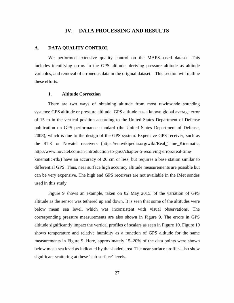
Figure 9 shows an example, taken on 02 May 2015, of the variation of GPS
altitude as the sensor was tethered up and down. It is seen that some of the altitudes were
below mean sea level, which was inconsistent with visual observations. The
corresponding pressure measurements are also shown in Figure 9. The errors in GPS
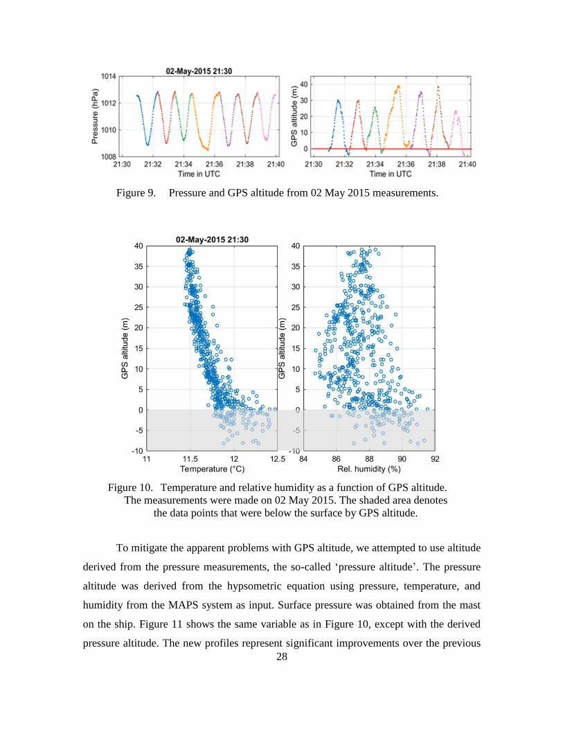
altitude significantly impact the vertical profiles of scalars as seen in Figure 10. Figure 10
shows temperature and relative humidity as a function of GPS altitude for the same
measurements in Figure 9. Here, approximately 15–20% of the data points were shown
below mean sea level as indicated by the shaded area. The near surface profiles also show
significant scattering at these ‘sub-surface’ levels.
28
Figure 9. Pressure and GPS altitude from 02 May 2015 measurements.
Figure 10. Temperature and relative humidity as a function of GPS altitude.
The measurements were made on 02 May 2015. The shaded area denotes
the data points that were below the surface by GPS altitude.
To mitigate the apparent problems with GPS altitude, we attempted to use altitude
derived from the pressure measurements, the so-called ‘pressure altitude’. The pressure
altitude was derived from the hypsometric equation using pressure, temperature, and
humidity from the MAPS system as input. Surface pressure was obtained from the mast
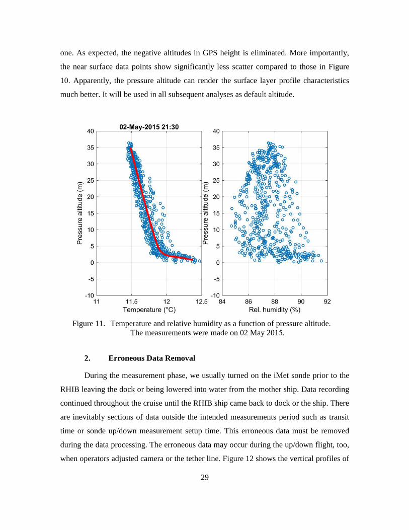
on the ship. Figure 11 shows the same variable as in Figure 10, except with the derived
pressure altitude. The new profiles represent significant improvements over the previous
29
one. As expected, the negative altitudes in GPS height is eliminated. More importantly,
the near surface data points show significantly less scatter compared to those in Figure
10. Apparently, the pressure altitude can render the surface layer profile characteristics
much better. It will be used in all subsequent analyses as default altitude.
Figure 11. Temperature and relative humidity as a function of pressure altitude.
The measurements were made on 02 May 2015.
2. Erroneous Data Removal
During the measurement phase, we usually turned on the iMet sonde prior to the
RHIB leaving the dock or being lowered into water from the mother ship. Data recording
continued throughout the cruise until the RHIB ship came back to dock or the ship. There
are inevitably sections of data outside the intended measurements period such as transit
time or sonde up/down measurement setup time. This erroneous data must be removed
during the data processing. The erroneous data may occur during the up/down flight, too,
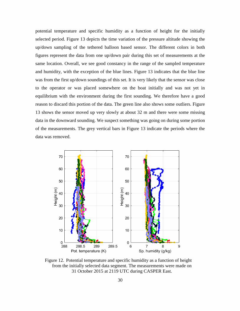
when operators adjusted camera or the tether line. Figure 12 shows the vertical profiles of
30
potential temperature and specific humidity as a function of height for the initially
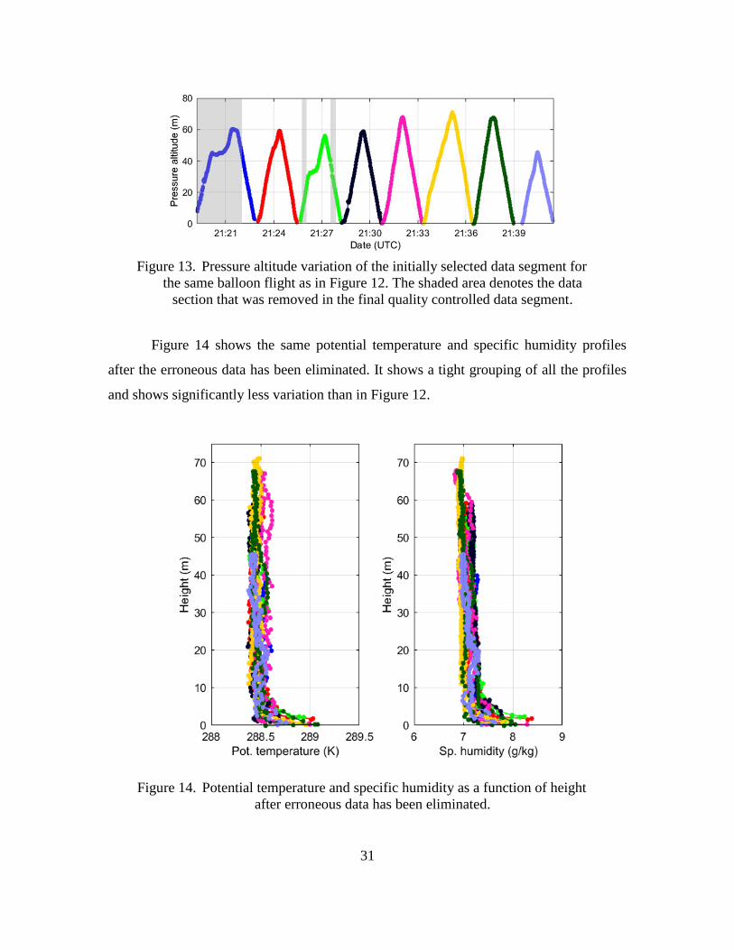
selected period. Figure 13 depicts the time variation of the pressure altitude showing the
up/down sampling of the tethered balloon based sensor. The different colors in both
figures represent the data from one up/down pair during this set of measurements at the
same location. Overall, we see good constancy in the range of the sampled temperature
and humidity, with the exception of the blue lines. Figure 13 indicates that the blue line
was from the first up/down soundings of this set. It is very likely that the sensor was close
to the operator or was placed somewhere on the boat initially and was not yet in
equilibrium with the environment during the first sounding. We therefore have a good
reason to discard this portion of the data. The green line also shows some outliers. Figure
13 shows the sensor moved up very slowly at about 32 m and there were some missing
data in the downward sounding. We suspect something was going on during some portion
of the measurements. The grey vertical bars in Figure 13 indicate the periods where the
data was removed.
Figure 12. Potential temperature and specific humidity as a function of height
from the initially selected data segment. The measurements were made on
31 October 2015 at 2119 UTC during CASPER East.
31
Figure 13. Pressure altitude variation of the initially selected data segment for
the same balloon flight as in Figure 12. The shaded area denotes the data
section that was removed in the final quality controlled data segment.
Figure 14 shows the same potential temperature and specific humidity profiles
after the erroneous data has been eliminated. It shows a tight grouping of all the profiles
and shows significantly less variation than in Figure 12.
Figure 14. Potential temperature and specific humidity as a function of height
after erroneous data has been eliminated.
32
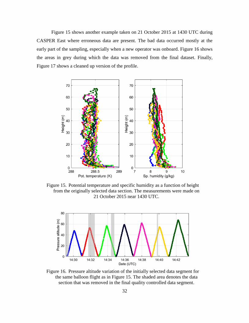
Figure 15 shows another example taken on 21 October 2015 at 1430 UTC during
CASPER East where erroneous data are present. The bad data occurred mostly at the
early part of the sampling, especially when a new operator was onboard. Figure 16 shows
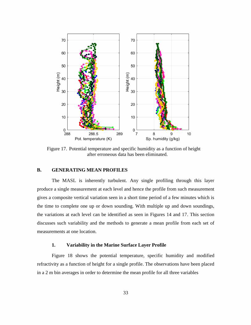
the areas in grey during which the data was removed from the final dataset. Finally,
Figure 17 shows a cleaned up version of the profile.
Figure 15. Potential temperature and specific humidity as a function of height
from the originally selected data section. The measurements were made on
21 October 2015 near 1430 UTC.
Figure 16. Pressure altitude variation of the initially selected data segment for
the same balloon flight as in Figure 15. The shaded area denotes the data
section that was removed in the final quality controlled data segment.
33
Figure 17. Potential temperature and specific humidity as a function of height
after erroneous data has been eliminated.
B. GENERATING MEAN PROFILES
The MASL is inherently turbulent. Any single profiling through this layer
produce a single measurement at each level and hence the profile from such measurement
gives a composite vertical variation seen in a short time period of a few minutes which is
the time to complete one up or down sounding. With multiple up and down soundings,
the variations at each level can be identified as seen in Figures 14 and 17. This section
discusses such variability and the methods to generate a mean profile from each set of
measurements at one location.
1. Variability in the Marine Surface Layer Profile
Figure 18 shows the potential temperature, specific humidity and modified
refractivity as a function of height for a single profile. The observations have been placed
in a 2 m bin averages in order to determine the mean profile for all three variables
34
Figure 18. Bin-averaged profile and its corresponding variability represented by
the standard deviation of the data point in each vertical bin. Potential
temperature, specific humidity, and the modified refractivity are shown in
this figure. The measurements were made on 15 October at 1222 UTC.
Figure 19 shows bin-averaged standard deviations of potential temperature and
specific humidity as a function of height from all CASPER-East MAPS profiles. The
figure shows that the standard deviation above 10 m is in general less than 0.3 oC for
potential temperature and 0.5 g kg-1
for specific humidity, although the standard
deviations varied significantly among different set of profiles. However, large variations
are seen in the lowest 10 m, where we expect large vertical gradient based on MOST
theory. Overall, the standard deviations in these lowest levels are less than 0.5 oC and 1.0
g kg-1
for potential temperature and specific humidity, respectively
35
Figure 19. Bin-averaged standard deviations of potential temperature and
specific humidity as a function of height. The values shown are composite
from all CASPER East profiles.
Figure 20 separates the calculated mean standard deviation of potential
temperature and specific humidity for all vertical bins of each profiling set obtained
during CASPER East. These vertically averaged variabilities seem to be rather consistent
from day-to-day and at different locations, except for the last few profiles obtained over
the Gulf Stream region. Figure 21 shows the same dataset separated by date of
measurements. One can see that the variability in each day from different locations has
about the magnitude as the day-to-day variation.
36
Figure 20. Mean standard deviation of potential temperature and specific
humidity from each MAPS sampling set during CASPER East. The
horizontal axis is the sequential sounding number.
Figure 21. Same as in Figure 20, except for using dates in local time as
horizontal axis.
In Figure 22, we examined how the profile mean variability differs with the
number of up/down profiles (each up/down of the balloon gives two profiles). There
appears to be no clear trend as to how the number of repeated profiles affect the sample
variability. In other words, the number of samples we used for these measurements seem
to be a sufficient representation.
37
Figure 22. Mean standard deviation of potential temperature and specific humidity from each MAPS sampling set during CASPER East. The
horizontal axis is the number of profiles taken for the particular set of profiles.
2. Methods to Generate Mean Profile
There are several methods developed to obtain the mean profile of the MASL from each MAPS profiling set. The first method, the bin averaged method, was discussed in the previous subsection. We used 2-m vertical bins for this analysis. The size of the bin gives enough samples within each bin and was small enough to allow the distinguishable difference in adjacent bins near the surface where the gradients are the largest. The second method uses polynomial fit of the dataset as a function of height. Polynomial fit is a curve fitting method where the data is approximated using a polynomial function. In this study, a 7th order polynomial function was used to determine the mean profiles. This higher order fit provides more flexibility in the shape of the profiles and allows the representation of a wide range of vertical variability. The third method, outlined in Kang and Wang (2016), is a least-squares optimization method that utilizes a weighted cost function based on the framework of MOST with the cost being optimized using a quasi-Newton method. The method assumes the samples are from the ensemble of profiles that follow MOST. All levels of the profile measurements are used and the method finds the profile that minimizes the cost function with a specialized weighting function. This
38
method incorporates all of the measurements in the derivations of the profiles and fluxes.
Details of this method are documented in Kang and Wang (2016).
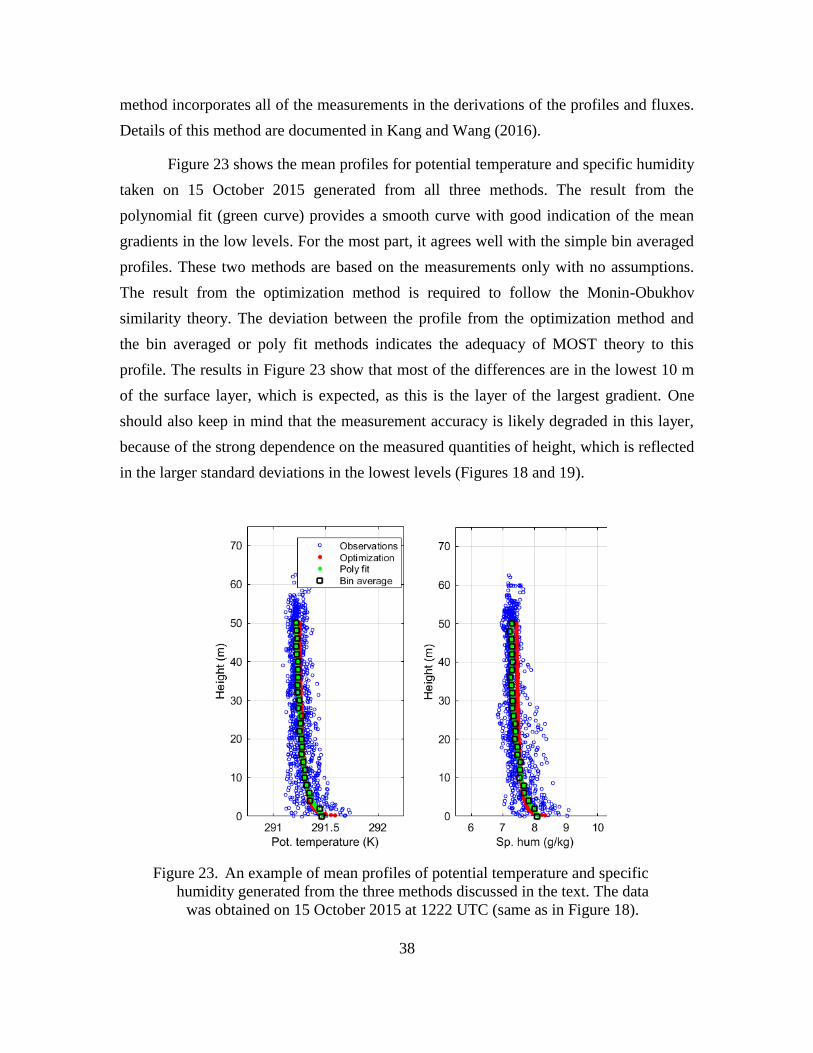
Figure 23 shows the mean profiles for potential temperature and specific humidity
taken on 15 October 2015 generated from all three methods. The result from the
polynomial fit (green curve) provides a smooth curve with good indication of the mean
gradients in the low levels. For the most part, it agrees well with the simple bin averaged
profiles. These two methods are based on the measurements only with no assumptions.
The result from the optimization method is required to follow the Monin-Obukhov
similarity theory. The deviation between the profile from the optimization method and
the bin averaged or poly fit methods indicates the adequacy of MOST theory to this
profile. The results in Figure 23 show that most of the differences are in the lowest 10 m
of the surface layer, which is expected, as this is the layer of the largest gradient. One
should also keep in mind that the measurement accuracy is likely degraded in this layer,
because of the strong dependence on the measured quantities of height, which is reflected
in the larger standard deviations in the lowest levels (Figures 18 and 19).
Figure 23. An example of mean profiles of potential temperature and specific
humidity generated from the three methods discussed in the text. The data
was obtained on 15 October 2015 at 1222 UTC (same as in Figure 18).
39
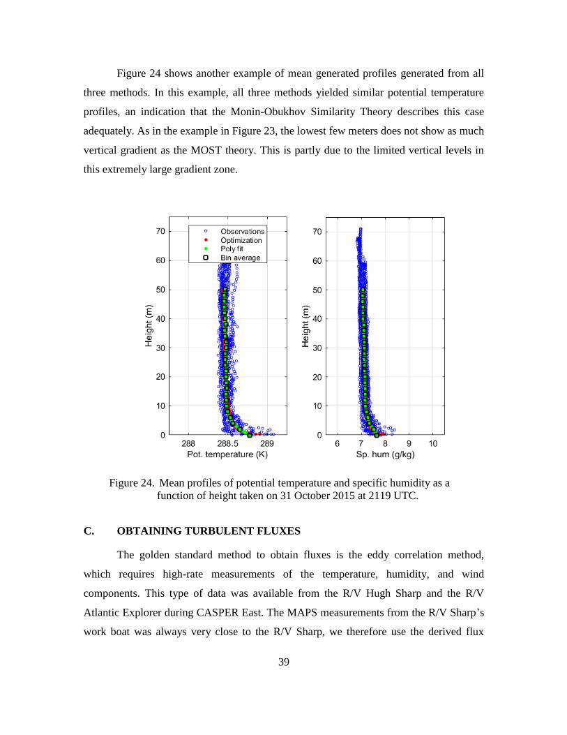
Figure 24 shows another example of mean generated profiles generated from all
three methods. In this example, all three methods yielded similar potential temperature
profiles, an indication that the Monin-Obukhov Similarity Theory describes this case
adequately. As in the example in Figure 23, the lowest few meters does not show as much
vertical gradient as the MOST theory. This is partly due to the limited vertical levels in
this extremely large gradient zone.
Figure 24. Mean profiles of potential temperature and specific humidity as a
function of height taken on 31 October 2015 at 2119 UTC.
C. OBTAINING TURBULENT FLUXES
The golden standard method to obtain fluxes is the eddy correlation method,
which requires high-rate measurements of the temperature, humidity, and wind
components. This type of data was available from the R/V Hugh Sharp and the R/V
Atlantic Explorer during CASPER East. The MAPS measurements from the R/V Sharp’s
work boat was always very close to the R/V Sharp, we therefore use the derived flux
40
from the high-rate measurements on the R/V Sharp to generate the true surface fluxes of
heat, water vapor, and momentum.
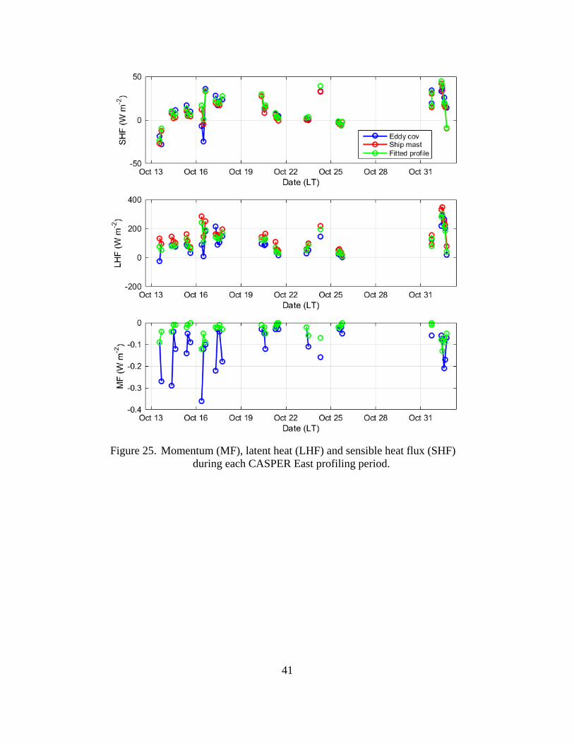
Turbulent fluxes can also be calculated using surface flux parameterization such as
the COARE algorithm. The input mean quantities can be obtained from the ship mast on
the R/V Sharp. We can also use the scalar quantities measured by the MAPS as input to the
COARE algorithm to obtain the parameterized surface fluxes. A comparison of the fluxes
with all three methods are shown in Figure 25. To calculate the fluxes from the mast we
used temperature, humidity and wind values obtained from the ships mast and input these
values into the COARE algorithm to obtain the parameterized flux values. To obtain the
fitted profile fluxes we used the mean values from our profile observations with the
exception of winds. Since the sonde is tethered, no measurements of winds were available
from the sonde measurements. As a result, the 12 m winds from the ships mast were used.
Hence, the parameterized fluxes from the mast and the MAPS use the same wind input,
which explains some of the similarities for fluxes from these methods (Figure 25).
41
Figure 25. Momentum (MF), latent heat (LHF) and sensible heat flux (SHF)
during each CASPER East profiling period.
42
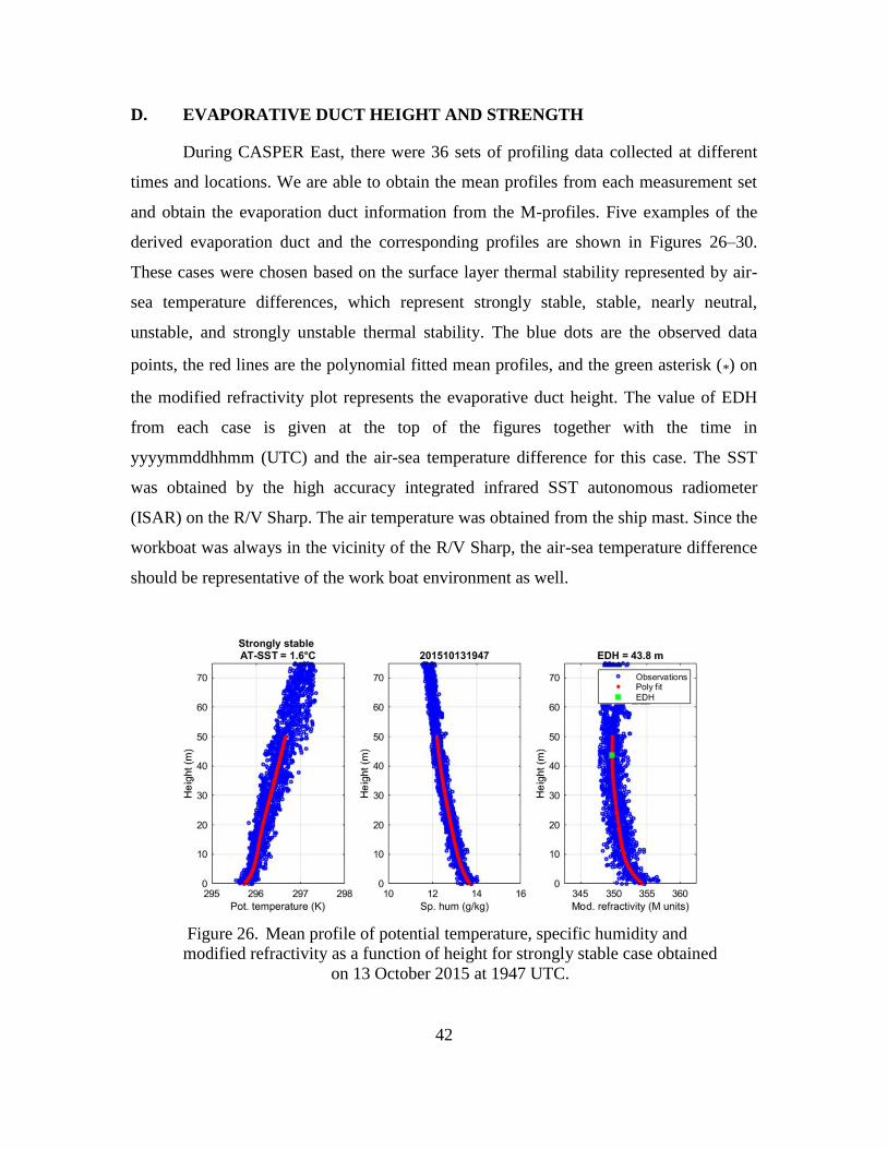
D. EVAPORATIVE DUCT HEIGHT AND STRENGTH
During CASPER East, there were 36 sets of profiling data collected at different
times and locations. We are able to obtain the mean profiles from each measurement set
and obtain the evaporation duct information from the M-profiles. Five examples of the
derived evaporation duct and the corresponding profiles are shown in Figures 26–30.
These cases were chosen based on the surface layer thermal stability represented by air-
sea temperature differences, which represent strongly stable, stable, nearly neutral,
unstable, and strongly unstable thermal stability. The blue dots are the observed data
points, the red lines are the polynomial fitted mean profiles, and the green asterisk (*) on
the modified refractivity plot represents the evaporative duct height. The value of EDH
from each case is given at the top of the figures together with the time in
yyyymmddhhmm (UTC) and the air-sea temperature difference for this case. The SST
was obtained by the high accuracy integrated infrared SST autonomous radiometer
(ISAR) on the R/V Sharp. The air temperature was obtained from the ship mast. Since the
workboat was always in the vicinity of the R/V Sharp, the air-sea temperature difference
should be representative of the work boat environment as well.
Figure 26. Mean profile of potential temperature, specific humidity and
modified refractivity as a function of height for strongly stable case obtained
on 13 October 2015 at 1947 UTC.
43
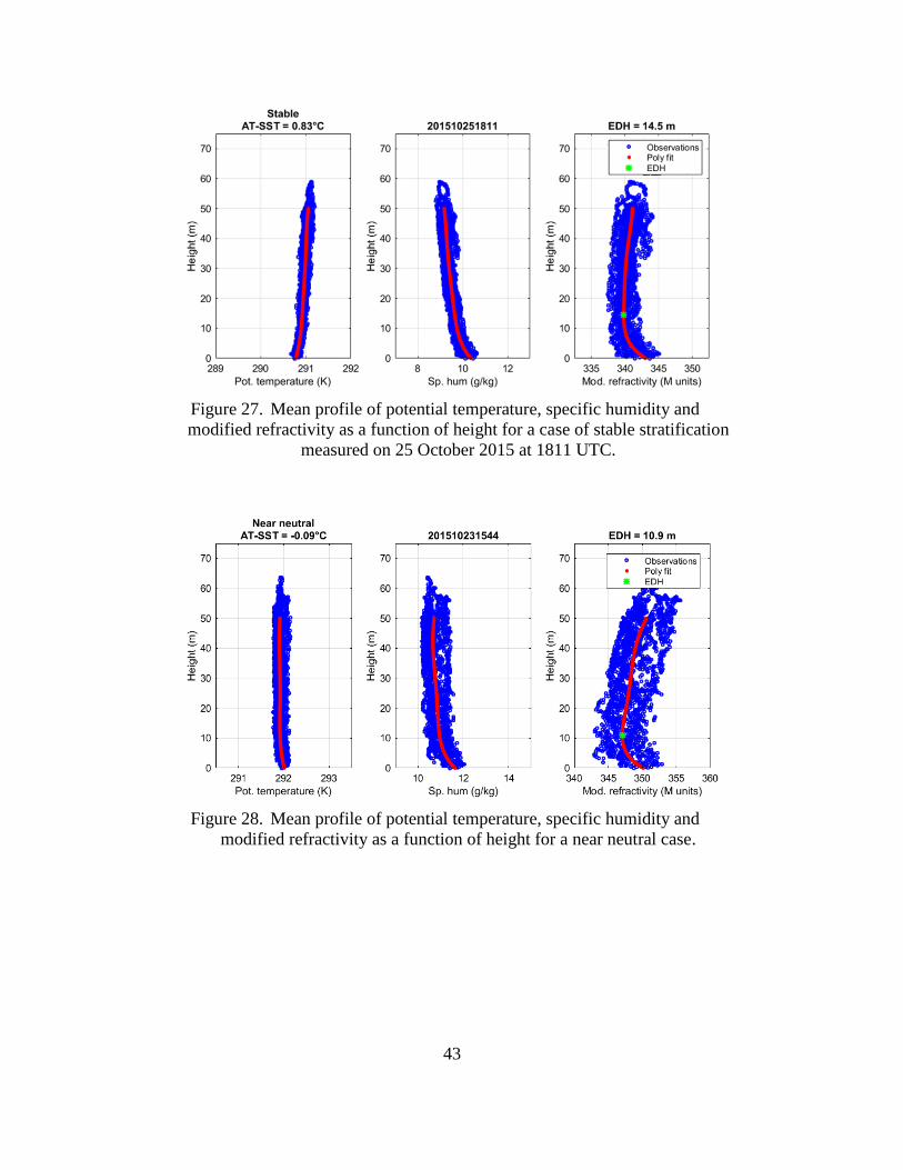
Figure 27. Mean profile of potential temperature, specific humidity and
modified refractivity as a function of height for a case of stable stratification
measured on 25 October 2015 at 1811 UTC.
Figure 28. Mean profile of potential temperature, specific humidity and
modified refractivity as a function of height for a near neutral case.
44
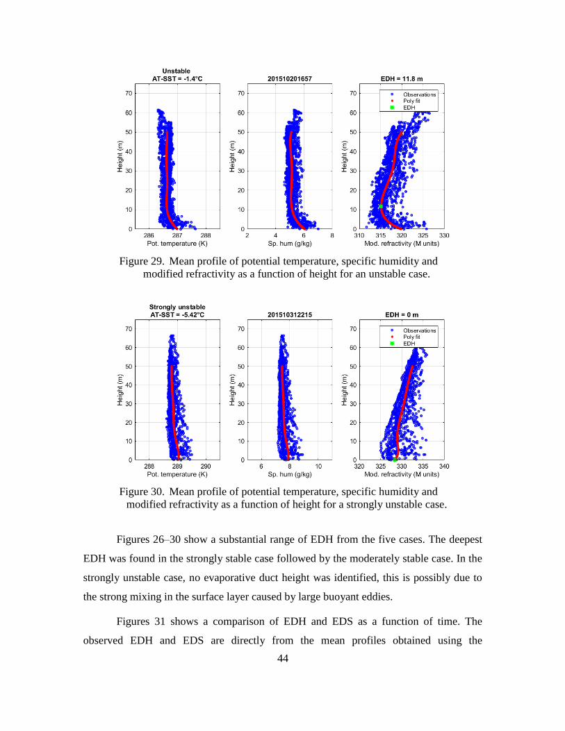
Figure 29. Mean profile of potential temperature, specific humidity and
modified refractivity as a function of height for an unstable case.
Figure 30. Mean profile of potential temperature, specific humidity and
modified refractivity as a function of height for a strongly unstable case.
Figures 26–30 show a substantial range of EDH from the five cases. The deepest
EDH was found in the strongly stable case followed by the moderately stable case. In the
strongly unstable case, no evaporative duct height was identified, this is possibly due to
the strong mixing in the surface layer caused by large buoyant eddies.
Figures 31 shows a comparison of EDH and EDS as a function of time. The
observed EDH and EDS are directly from the mean profiles obtained using the
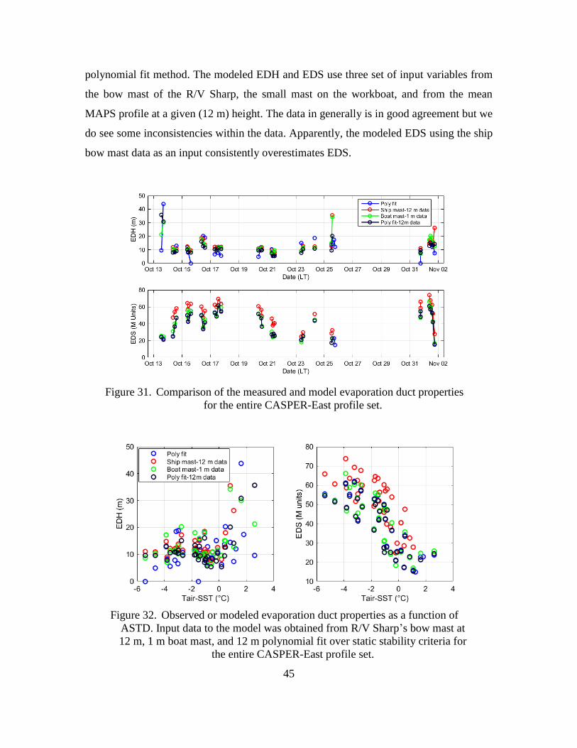
45
polynomial fit method. The modeled EDH and EDS use three set of input variables from
the bow mast of the R/V Sharp, the small mast on the workboat, and from the mean
MAPS profile at a given (12 m) height. The data in generally is in good agreement but we
do see some inconsistencies within the data. Apparently, the modeled EDS using the ship
bow mast data as an input consistently overestimates EDS.
Figure 31. Comparison of the measured and model evaporation duct properties
for the entire CASPER-East profile set.
Figure 32. Observed or modeled evaporation duct properties as a function of
ASTD. Input data to the model was obtained from R/V Sharp’s bow mast at
12 m, 1 m boat mast, and 12 m polynomial fit over static stability criteria for
the entire CASPER-East profile set.
46
Figure 32 shows the same evaporation duct properties as in Figure 31, except as a
function of air-sea temperature difference (ASTD). Negative ASTD denotes unstable
stratification, positive for stable stratification. Here, we observe small variability of the
EDH in the unstable conditions and strong sensitivity in stable conditions. This result is
consistent with the findings of Cherrett (2015) using the COARE algorithm. However,
there was still a lack of observational data in the stable regime. The measured EDS
follows the MOST calculated values well and indicated weak ducts in stable conditions
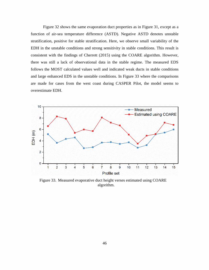
and large enhanced EDS in the unstable conditions. In Figure 33 where the comparisons
are made for cases from the west coast during CASPER Pilot, the model seems to
overestimate EDH.
Figure 33. Measured evaporative duct height verses estimated using COARE
algorithm.
47
V. SUMMARY AND CONCLUSIONS
A. NPS MAPS CONCLUSIONS
Accurate depiction of the temperature, humidity, and wind profiles in the MASL
are critical in quantifying the effects of the atmosphere on electromagnetic wave
propagation and in particular evaporative ducts. However, the vertical profiles in the
lowest 50 m of the atmosphere have not been well measured because of the impact of the
large ships or platforms on their immediate environment. NPS has developed a Marine
Atmospheric Profiling System (MAPS) that is capable of making repeated measurements
of the MASL in a relatively undisturbed environment. The MAPS is comprised of a MET
mast, tethered balloon, a radiosonde and receiving and data display package along with a
sea surface thermistor. The system is designed to obtain surface layer profiles as well as
one level of wind for data retrieval and analysis later on. The system prototype was tested
in CAPER-Pilot and improved in CASPER-East, 15 data sets were made during
CASPER-Pilot and 36 during CASPER-East.
Careful data quality control was applied to the MAPS profiles. Issues with GPS
altitude were identified that may introduce the structure and characteristics of the profiles
considerably. This problem was resolved by using pressure altitude. Erroneous data,
mostly in the beginning of the data collection at each location, was removed by using
prior knowledge of the problem domain and by using common sense. The variability of
the MASL temperature and humidity at each level was clearly seen from multiple
up/down measurements at a single location. These variations are result of the natural
variability in a turbulent environment, which points out to potentially large uncertainties
in using a single vertical profile to represent the mean atmospheric conditions. The mean
profile and its variability was obtained by sectioning the vertical dimension into 2-m
depth bins and calculate the mean and variance in each bin. The bin-averaged vertical
profiles clearly showed the near surface gradients in both temperature and humidity,
which allowed us to identify the evaporation duct properties from the derived mean
modified refractivity profile. The variances of potential temperature and specific
humidity did not change significantly with height above the surface and are consistent
48
for most of the profiles with the exception of profiles taken over the Gulf Stream on 01
November 2015. The variances also did not vary significantly for different number of
sample profiles. In addition to the simple bin averaging approach, a polynomial fit of the
data points were also attempted to generate the ‘mean’ profile. The 7th
order polynomial
fit and the bin average method gave rather consistent profiles. In addition, Kang and
Wang (2016) introduced a least-square optimization method that fit the data points to a
profile that followed the MOST in the surface layer. This method was also applied to the
CASPER East and some of the CASPER Pilot profiles. Good comparison between this
method and the purely observation based profiles indicate the validity of the MOST
theory, which is the case in some of the profiles. However, there are also profiles that
showed significant deviations.
Using data from a specific level on the MAPS profiles as an input to surface flux
parameterization algorithms, one can obtain surface fluxes of sensible and latent heat.
Fluxes generated this way compared well with those from the eddy correlation method or
the parameterized fluxes using measurements from the bow mast on the R/V Sharp near
by the workboat during CASPER East. Since the wind speed used in the parameterized
flux calculation was the same, the good comparison of the parameterization essentially
reveals that the mean temperature and specific humidity from the ship bow mast and the
MAPS profile at the bow mast level are consistent. The good comparison between the
eddy covariance and the parameterized fluxes suggest the validity of the COARE flux
algorithm, which was used in calculating fluxes from the mean measurements.
The main objective of developing the MAPS is to obtain directly measured
evaporation duct properties. Using the surface layer profiles from CASPER East and
CASPER Pilot field campaigns, we were able to obtain evaporation ducts properties in
different stability and wind conditions shown in five examples in this thesis. Shallow but
strong ducts were found in the unstable surface layers and deep but weak ducts were
found in the stable surface layers. The measured evaporation duct properties can be used
to evaluate evaporation duct models. In this thesis, we used the modified COARE
algorithm to derived the modeled evaporation ducts. A Comparison of measured
evaporative duct height with COARE surface layer model estimated evaporative duct

49
height from CASPER pilot experiment showed that model generally overestimated the
duct heights in cases during CASPER pilot. No persistent trend of the model-observation
comparison was observed for cases obtained during CASPER East. Further in-depth
analyses are needed with this dataset to identify the conditions where evaporation models
need further improvements.
B. RECOMMENDATIONS FOR FUTURE WORK
The NPS MAPS is fully developed and functions very well in CASPER pilot
testing and during CASPER East. We have also developed methods to obtain mean
temperature and humidity profiles for calculation of the mean evaporation duct height.
Future work should be associated with the use of the system and deploying it in different
conditions so that more data can contribute to a better understanding of the evaporative
duct modeling.

50
THIS PAGE INTENTIONALLY LEFT BLANK

51
LIST OF REFERENCES
Andreas, E., P. O. G. Persson, J. E. Hare, 2008: bulk turbulent air-sea flux algorithm for
high-wind, spray conditions. J. Phys. Oceanogr., 38, 1581–1596.
Babin, S. M., G. S. Young, and J. A. Carton, 1997: A new model of the
oceanicevaporation duct. J. Appl. Meteor., 36, 193–204.
Bean, B. B., and E. J. Dutton, 1968: Radio Meteorology. Dover Publications, 435 pp.
Babin, S. M., G. S. Young, and J. A. Carton, 1997: A new model of the oceanic
evaporation duct. J. Appl. Meteor., 36, 193–204.
Blackadar, A.K., 1993: The vertical distribution of wind and turbulent exchange in a
neutral atmosphere. J. Geophys. Res., 67, 3095–3102.
Businger, J. A., J. C., Wyngaard, Y. Izumi, and E. F. Bradley, 1971: Flux-profile
relationships in the atmospheric surface layer. J. Atmos. Sci., 28, 181–189.
Charnock, H., 1955: Wind stress on a water surface. Quart. J. Roy. Meteor. Soc., 81,
639–640.
Cherrett, R.C., 2015: Capturing characteristics of atmospheric refractivity using
observation and modeling approaches. Dissertation, Naval Postgraduate School,
30–32 pp..
Cook, J., & Burk, S. (1992): Potential refractivity as a similarity variable. Bound.-Layer
Meteor, 58(1-2), 151–159.
Dockery, G. D., 1988: Modeling electromagnetic wave propagation in the troposphere
using the parabolic equation. IEEE Trans. Antennas Propag., 36, 1464–1470.
Edson, J. B., C. J. Zappa, J. A. Ware, W. R. McGillis, and J. E. Hare, 2004: Scalar flux
profile relationships over the open ocean, J. Geophys. Res., 1–15.
Edson, J. B., T. Paluszkiewicz, S. Sandgathe, L. Vincet, L. Goodman, T. Curtin, J.
Hollister, and M. Coulton, 1999: Coupled marine boundary layers and air-sea
interaction initiative: Combining process studies, simulations, and numerical
models. [Available online at http://www.whoi.edu/science/AOPE/dept/r5.pdf.]
Fairall, C. W., E. F. Bradley, D. P. Rogers, J. B. Edson, and G. S. Young, 1996: Bulk
parameterization of air–sea fluxes for Tropical Ocean and Global Atmosphere
Coupled Ocean–Atmosphere Response Experiment. J. Geophys. Res., 101,
3747–3764.
52
Fairall, C. W., E. F. Bradley, J. E. Hare, A. A. Grachev, and J. B. Edson, 2003: Bulk
parameterization of air-sea fluxes: Updates and verification for COARE
algorithm. J. Climate, 16, 571–591.
Frederickson, P., K. Davidson, J. Stapleton, D. Shanklin, R. Wiss, T. Nguyen, E. Burgess
III, C. Weeks, W. Thornton, and T. Brown, 2012: Validation of AREPS
propagation assessments using different evaporation duct models. Naval
Postgraduate School, draft, 23 pp.
Frederickson, P. A., K. L. Davidson, and A. K. Goroch, 2000: Operational bulk
evaporation duct model for MORIAH,. Naval Postgraduate School, Draft Version
1.2, May 2000, 70 pp.
Gallaudet T, 2016, Naval Oceanography Electromagnetic Maneuver Warfare Strategy
Accessed 12 March 2016. [Available online at
http://www.navy.mil/submit/display.asp?story_id=93788].
Gehman, J. Z., 2000: Importance of evaporation duct stability in propagation-sensitive
studies. JHU APL Tech. Rep. A2A-00-U-3-008, 8 pp.
Jeske, H., 1973: State and limits of prediction methods of radar wave propagation
conditions over the sea. Modern Topics in Microwave Propagation and Air–Sea
Interaction, A. Zancla, Ed., D. Reidel Publishing, 130–148.
Kang, D., and Q. Wang, 2016: Optimized estimation of surface layer characteristics from
profiling measurements. Article, Atmosphere, 7, pp 1–6.
Liu, T., Katsaros, and J. A. Businger, 1979: The Liu, Katsaros, and Businger Bulk
Atmospheric Flux Computational Iteration Program in Fortran and Basic. NRL
Memorandum Report 5291, AD-A156,736 pp.
Liu, W. T., and T. V. Blanc, 1984: Liu, Katsaros, and Businger (1979) bulk atmospheric
flux computational iteration program in FORTRAN and BASIC. United States
Naval Research Lab., Wash., D.C., NRL Memorandum Report 5291, May 8,
1984, 20.
Paulus, R. A., 1984: Practical application of the IREPS evaporation duct model.
NOSCTech. Rep. 966, 68 pp. [Available from National Technical Information
Service, U.S. Department of Commerce, Technology Administration, 5285 Port
Royal Road, Springfield, VA 22161.]
Paulus, R. A., 1985: Practical application of an evaporation duct model. Radio Sci., 20,
887–896.
Paulus, R. A., 1989: Specification for Environmental Measurements to Assess
RadarSensors. NOSC Tech Document 1685, 43 pp. [Available from National

53
Technical Information Service, U.S. Department of Commerce, Technology
Administration, 5285 Port Royal Road, Springfield, VA 22161.]
Stull, R. B., 1988: An introduction to boundary layer meteorology. Dordrecht, Holland,
Kluwer Academic Publishers, 666 pp.
Tellado, P. A., 2013: Physical Processes in Coastal Stratocumulus Clouds from Aircraft
Measurements during UPPEF 2012. M. S. thesis, Dept. of Meteorology, Naval
Postgraduate School, pp.5–12.
Turton, J. D., D. A. Bennets, and S. F. G. Farmer, 1988: An introduction to radio ducting.
Meteor. Mag., 17, 245–254
United States Department of Defense, 2008: Global positioning system standard
positioning service performance standard. Accessed 05 May 2016. [Available
online at
https://en.wikipedia.org/wiki/Real_Time_Kinematic,%20http:/www.novatel.com/
an-introduction-to-gnss/chapter-5-resolving-errors/real-time-kinematic-rtk/].
Wang Q., R. Burkholder, J. Fernando, D Khelif, R. K Shearman, and L Shen, 2015:
CASPER—A new multidisciplinary research initiative on electromagnetic wave
propagation in the marine atmosphere, Radio Science Meeting (Joint with AP-S
Symposium), 2015 USNC-URSI, Vancouver, BC, Canada, 2015, pp. 252–252.
Zandbergen, P A., and S. J. Barbeau, 2011: Positional accuracy of assisted GPS data from
high-sensitivity GPS-enabled mobile phones. Journal of Navigation, 64, pp 381–
399.

54
THIS PAGE INTENTIONALLY LEFT BLANK

55
INITIAL DISTRIBUTION LIST
1. Defense Technical Information Center
Ft. Belvoir, Virginia
2. Dudley Knox Library
Naval Postgraduate School
Monterey, California


![Carrier-to-Noise-Threshold Filtering on Off-Shore Wind ... · 300 m instrumented masts exists, e.g., the 280 m instrumented TV tower Hamburg [11,12], the 200 m meteorological mast](https://img.pdfslide.net/doc/110x75/60608282c2150c043231ef7c/carrier-to-noise-threshold-filtering-on-off-shore-wind-300-m-instrumented-masts.jpg)