Navigation Techniques for Environmental Technicians · Web viewEnvironmental Monitoring & Technology Series Noise monitoring & evaluation For Technicians Study module 2 Introduction

cffet.net/env

Noise monitoring & evaluationFor Technicians

Study module 2Introduction

Environmental Monitoring & Technology Series

Noise monitoring & evaluation Study Module 2

Assessment details

PurposeThis subject covers the ability to site and set up basic ‘ground level’ meteorological equipment and collect and record reliable data. It also includes the ability to assess data quality, interpret significant data features and use the data to ensure the validity of air and noise monitoring measurements.

Instructions◗ Read the theory section to understand the topic.◗ Complete the Student Declaration below prior to starting.◗ Attempt to answer the questions and perform any associated tasks.◗ Email, phone, book appointment or otherwise ask your teacher for help if required.◗ When completed, submit task by email using rules found on last page.

Student declarationI have read, agree to comply with and declare that;

◗ I know how to get assistance from my assessor if needed… ☐◗ I have read and understood the SAG for this subject/unit… ☐◗ I know the due date for this assessment task… ☐◗ I understand how to complete this assessment task… ☐◗ I understand how this assessment task is weighted… ☐◗ I declare that this work, when submitted, is my own… ☐

DetailsStudent name Type your name here

Assessor Type teachers name here

Class code NME

Assessment name SM2

Due Date Speak with your assessor

Total Marks Available 34

Marks Gained Marker’s use only

Final Mark (%) Marker’s use only

Marker’s Initials Marker’s use only

Date Marked Click here to enter a date.

Weighting This is one of six formative assessments and contributes 10% of the overall mark for this unit

Hunter TAFE - Chemical, Forensic, Food & Environmental Technology [cffet.net/env] Course Notes for delivery of MSS11 Sustainability Training Package Page | 1


Chapter 2 – Acoustic theory

This section outlines the science behind sound. For those of you that actually enjoy science, then this will be a somewhat basic introduction into one small part of the world of physics. To those of you who don’t like science much, this part will…is compulsory to learn!

The basic physics of soundThe keys to understanding the acoustics of sound or noise lies in understanding pressure, which is a topic that should be familiar to you from previous study, but, along with time and distance shall be briefly revisited here, as well as understanding the properties of a wave in general.

Types of waves and their formationPressure, such as with atmospheric pressure, is the quotient of force and area, where force is measured in unit Newton. So if you apply a force over an area, you create pressure, whose unit is the Pascal, Pa. Sounds are merely a repeating of this process, which results in a pressure wave, which when heard is called a sound wave (although there are pressure waves we cannot hear). The pressure (sound) wave travels in a direction over a distance (which is usually measured in meters, m) over a period of time, t, measured in seconds, s.

Pressure travels in waves. Pressure waves we can hear are called sound waves. A sound wave is a pressure wave and vice versa.

Sound is caused when fluctuations in air pressure give rise to pressure waves which travel through a medium such as the atmosphere (but the medium can be any material). As the waves travel they will interact in various ways with their surroundings which tends to complicate things drastically, luckily though it is possible to describe the behaviour of sound in simple, idealized situations, and to use these to a better understanding of how it all works in the real world.

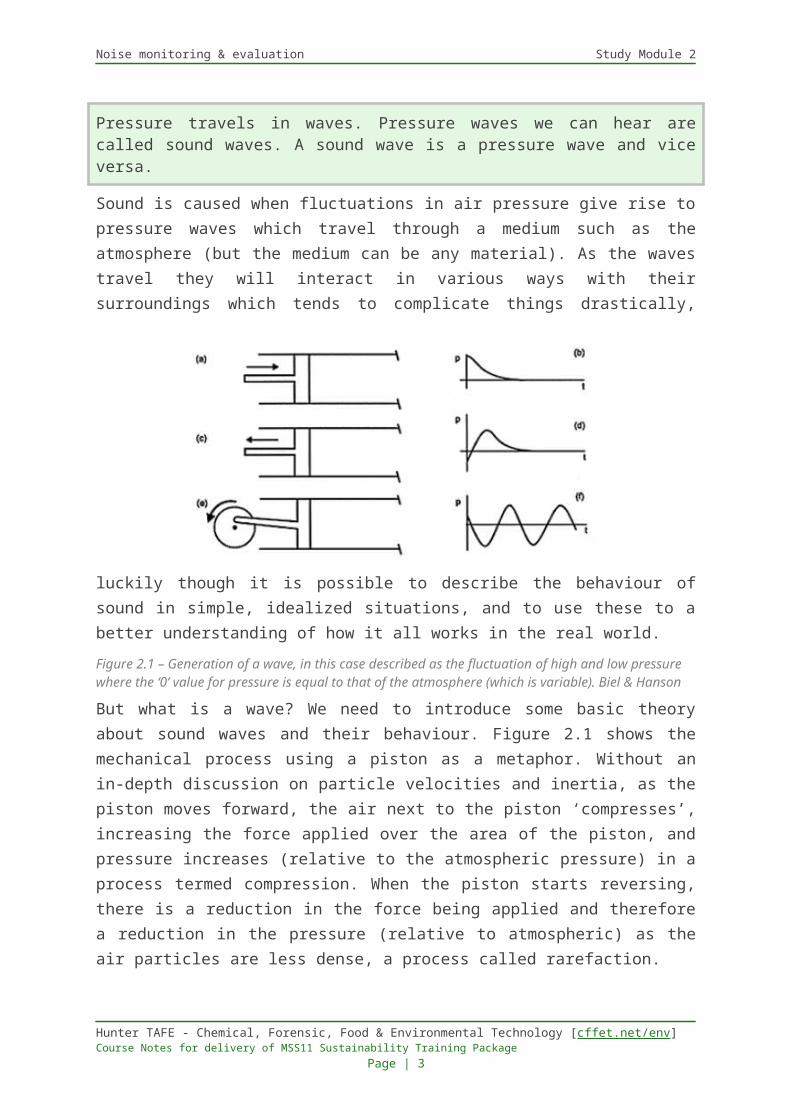
Figure 2.1 – Generation of a wave, in this case described as the fluctuation of high and low pressure where the ‘0’ value for pressure is equal to that of the atmosphere (which is variable). Biel & Hanson



But what is a wave? We need to introduce some basic theory about sound waves and their behaviour. Figure 2.1 shows the mechanical process using a piston as a metaphor. Without an in-depth discussion on particle velocities and inertia, as the piston moves forward, the air next to the piston ‘compresses’, increasing the force applied over the area of the piston, and pressure increases (relative to the atmospheric pressure) in a process termed compression. When the piston starts reversing, there is a reduction in the force being applied and therefore a reduction in the pressure (relative to atmospheric) as the air particles are less dense, a process called rarefaction.

The overall result is a cycle of positive and negative pressure fluctuations, and if we were to graph this process after several cycles we would see a graph in the shape of a sine wave, as seen in Figure 2.1.

Wave behaviourFigure 2.1 shows the formation of a ‘wave’, but there is more to it than this as there are two different types of wave (of interest to us); the longitudinal and the transverse.

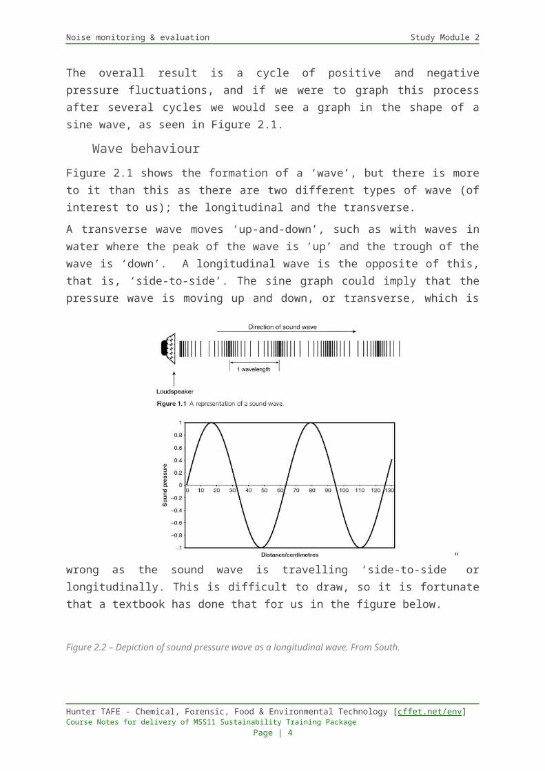
A transverse wave moves ‘up-and-down’, such as with waves in water where the peak of the wave is ‘up’ and the trough of the wave is ‘down’. A longitudinal wave is the opposite of this, that is, ‘side-to-side’. The sine graph could imply that the pressure wave is moving up and down, or transverse, which is wrong as the sound wave is travelling ‘side-to-side” or longitudinally. This is difficult to draw, so it is fortunate that a textbook has done that for us in the figure below.

Figure 2.2 – Depiction of sound pressure wave as a longitudinal wave. From South.



Wave properties

A wave has a number of significant properties, all of which will be explored in this section. The basic attributes that we will consider are amplitude, wavelength, time, distance, frequency and the speed of sound (velocity, which most of the time we shall assume is constant).

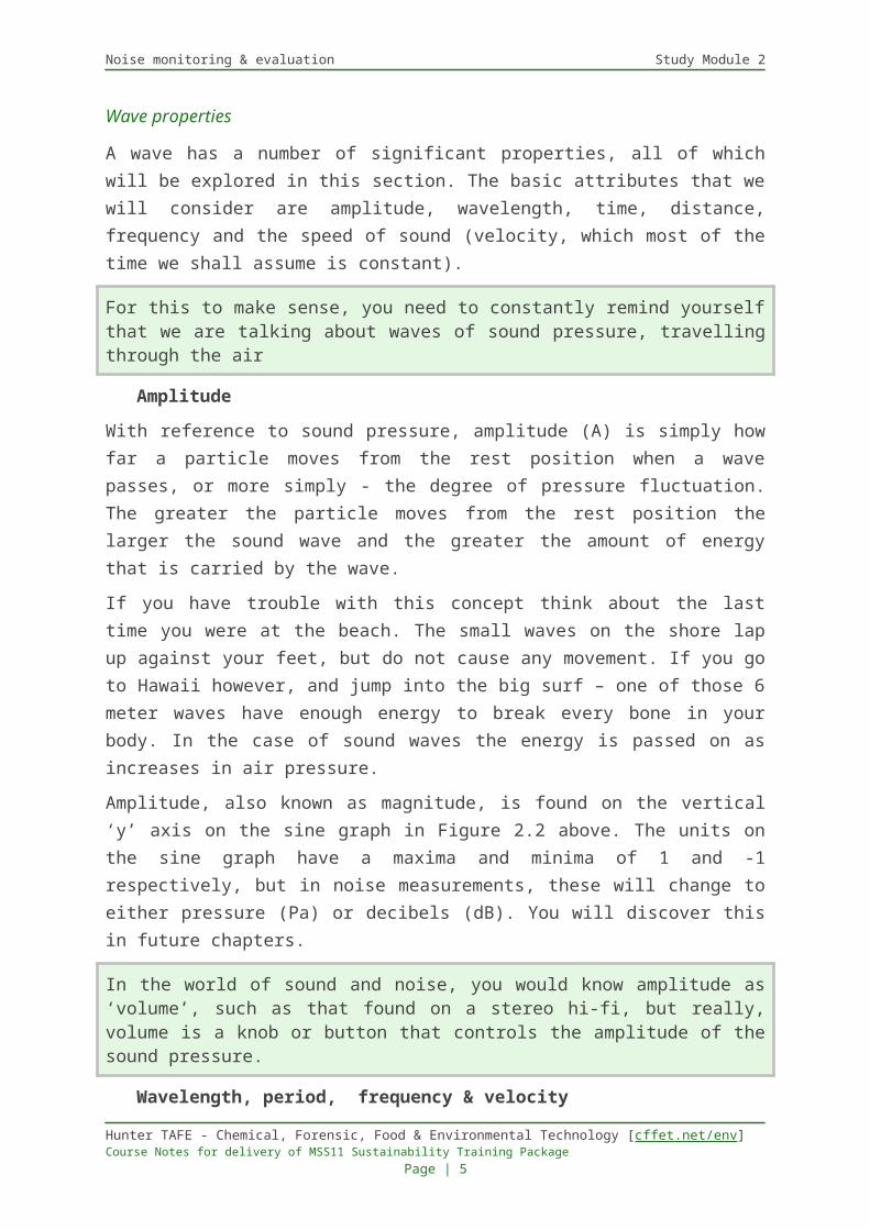
For this to make sense, you need to constantly remind yourself that we are talking about waves of sound pressure, travelling through the air

Amplitude

With reference to sound pressure, amplitude (A) is simply how far a particle moves from the rest position when a wave passes, or more simply - the degree of pressure fluctuation. The greater the particle moves from the rest position the larger the sound wave and the greater the amount of energy that is carried by the wave.

If you have trouble with this concept think about the last time you were at the beach. The small waves on the shore lap up against your feet, but do not cause any movement. If you go to Hawaii however, and jump into the big surf – one of those 6 meter waves have enough energy to break every bone in your body. In the case of sound waves the energy is passed on as increases in air pressure.

Amplitude, also known as magnitude, is found on the vertical ‘y’ axis on the sine graph in Figure 2.2 above. The units on the sine graph have a maxima and minima of 1 and -1 respectively, but in noise measurements, these will change to either pressure (Pa) or decibels (dB). You will discover this in future chapters.

In the world of sound and noise, you would know amplitude as ‘volume’, such as that found on a stereo hi-fi, but really, volume is a knob or button that controls the amplitude of the sound pressure.

Wavelength, period, frequency & velocity

The wave created by the sound (independent of amplitude) will travel over a distance. The unit of distance used in sound measures is the meter (m). The distance travelled will take a certain amount of time, which is measured in seconds (s). So we have time and distance intertwined in a unique relationship, which can be expressed using the following equation;

ν=fλ

Where;

V = velocity (m/s)

F = frequency (c/s)

L = wavelength (m)

Albeit, it is sometimes necessary to look a bit further into this simple equation to see all of its magic. Examine the worked example below;



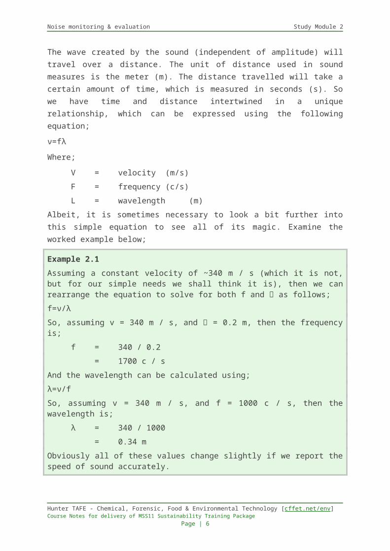
Example 2.1

Assuming a constant velocity of ~340 m / s (which it is not, but for our simple needs we shall think it is), then we can rearrange the equation to solve for both f and as follows;

f=ν/λ

So, assuming v = 340 m / s, and = 0.2 m, then the frequency is;

f = 340 / 0.2

= 1700 c / s

And the wavelength can be calculated using;

λ=ν/f

So, assuming v = 340 m / s, and f = 1000 c / s, then the wavelength is;

λ = 340 / 1000

= 0.34 m

Obviously all of these values change slightly if we report the speed of sound accurately.

Sometimes this concept is best seen pictorially, as seen in Figure 2.3 below where other concepts are explained such as the period etc.

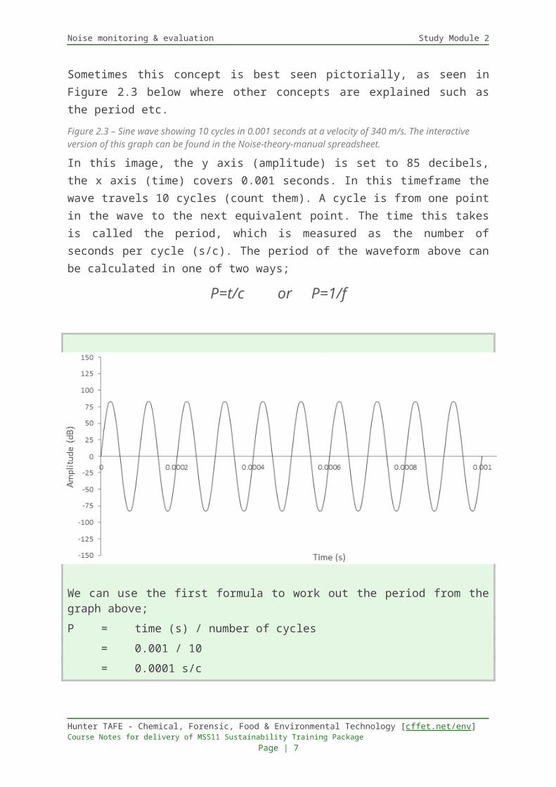
Figure 2.3 – Sine wave showing 10 cycles in 0.001 seconds at a velocity of 340 m/s. The interactive version of this graph can be found in the Noise-theory-manual spreadsheet.

In this image, the y axis (amplitude) is set to 85 decibels, the x axis (time) covers 0.001 seconds. In this timeframe the wave travels 10 cycles (count them). A cycle is from one point in the wave to the next equivalent point. The time this takes is called the period, which is measured as the number of seconds per cycle (s/c). The period of the waveform above can be calculated in one of two ways;

P=t/c or P=1/f



We can use the first formula to work out the period from the graph above;

P = time (s) / number of cycles

= 0.001 / 10

= 0.0001 s/c

The frequency is described as the reciprocal of the period, that is the number of cycles per second, which is actually far more informative than the period is, so it is the frequency that is usually calculated from such things and is expressed in the unit of Hertz (Hz) The frequency can therefore be calculated as;

f=1/PFrom the information above, this is calculated as;

f = 1 / P

= 1 / 0.0001

= 10000 c/s (Hz)

The wavelength is the length of one period of the waveform, which is from one point in the wave to the next equivalent point, and as mentioned is measured in meters (m). Now that we know the frequency, we can calculate the wavelength assuming a velocity of 340 m/s;

λ = v / f

= 340 / 10000

= 0.034 m

The sine wave

Now that you know the basics of waves, we can move on to slightly more complex issues. A sine wave, in its most simple form can be constructed from the following formula;

u=A∙sin((2πft)-θ)Where;

u = position of a point in the waveA = Amplitude, i.e. 'height' of the wave from the centersin = Excel's SIN (sinusoidal) functionπ = Excel's PI functionf = Frequency, as Hz or c/s or s-1

t = Time, secondsΘ = Phase, or 'offset', sort of irrelevant to us.

Relax, you don’t need to know how to use this formula, you just need to be aware that a whole heap of information can be derived from it.



From this, we can calculate several other important variables such as the period, time, wavelength, angular frequency, wavenumber and the list could go on. The important variables are found below;

ω = 2πf Calculates the angular frequency (r/s)

T = 2πω Calculates the period (seconds per wave s/ λ)

λ = ν/f Calculates the wavelength in meters (m)

k = 2π/ λ Calculates the angular wavenumber (r/ λ)

Interactive spreadsheet

Now would be a good time to work with the sine wave simulator in the interactive spreadsheet called Noise-theory-manual on the Physics 3 tab. This will allow you to visualise the sine wave and its properties in action.

The sine wave and its phase shifted cousin the cosine, are very important in science, and go a long way to explaining the behaviour of sound and noise. In the world of sound, the sine wave in Figure 2.3 above would represent a phenomena known as a pure tone, which is a ‘perfect sound’, and although rarely (if ever) found in nature, the pure tone can be generated on a device called an oscilloscope.

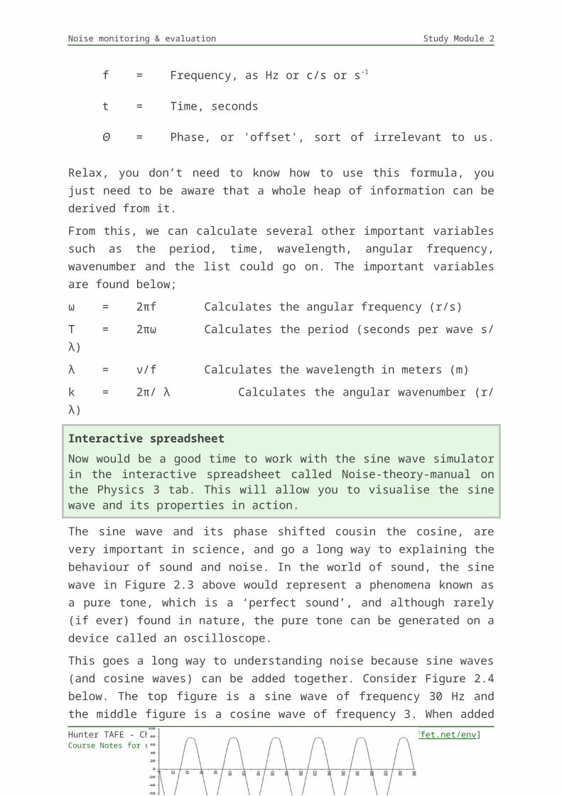
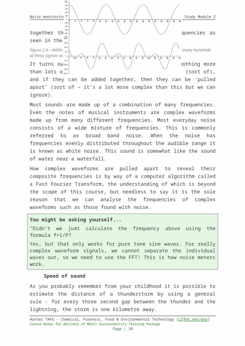
This goes a long way to understanding noise because sine waves (and cosine waves) can be added together. Consider Figure 2.4 below. The top figure is a sine wave of frequency 30 Hz and the middle figure is a cosine wave of frequency 3. When added together they make a new sound with multiple frequencies as seen in the bottom figure.



Figure 2.4 – Adding sine and cosine waves to get a ‘noisier’ signal. Imagine noise as many hundreds of these signals added together. From Noise-theory-manual spreadsheet.

It turns out that complex waveforms of noise are nothing more than lots of sine and cosine waves ‘added together’ (sort of), and if they can be added together, then they can be ‘pulled apart’ (sort of – it’s a lot more complex than this but we can ignore).

Most sounds are made up of a combination of many frequencies. Even the notes of musical instruments are complex waveforms made up from many different frequencies. Most everyday noise consists of a wide mixture of frequencies. This is commonly referred to as broad band noise. When the noise has frequencies evenly distributed throughout the audible range it is known as white noise. This sound is somewhat like the sound of water near a waterfall.

How complex waveforms are pulled apart to reveal their composite frequencies is by way of a computer algorithm called a Fast Fourier Transform, the understanding of which is beyond the scope of this course, but needless to say it is the sole reason that we can analyse the frequencies of complex waveforms such as those found with noise.

You might be asking yourself...

“Didn’t we just calculate the frequency above using the formula f=1/P?”

Yes, but that only works for pure tone sine waves. For really complex waveform signals, we cannot separate the individual waves out, so we need to use the FFT! This is how noise meters work.

Speed of sound

As you probably remember from your childhood it is possible to estimate the distance of a thunderstorm by using a general rule - for every three second gap between the thunder and the lightning, the storm is one kilometre away.

To be more accurate we can say that the speed with which sound spreads throughout a medium depends on the mass and elastic properties of the medium. In air at around 25C, sound travels at around 340 m/sec. (or 1224 km/hr). In other media such as water speeds are different.

Sound generally moves much faster in liquids and solids than in gases. The speed of sound in water, for example, is slightly less than 1,525 m/sec at ordinary temperatures but increases greatly with an increase in temperature. The speed of sound in copper is about 3,353 m/sec at ordinary temperatures and decreases as the temperature is increased (owing to decreasing elasticity); in steel, which is more elastic, sound moves at a speed of about 4,877 m/sec. Sound is propagated very efficiently in steel.

We can calculate the speed of sound using a variety of methods. The first method is to use the frequency-wavelength equation from above (v = fl), for which we need to know the frequency and the wavelength, yet speed of sound can be calculated from other data as well, with the easiest formula taking the form of;



v=(331.3+0.606∙T)Where T = the atmospheric temperature on degrees Celsius.

Example

Calculate the difference in the speed of sound for 12°C & 42°C.

V = (331.3 + 0.606 x 12)

= (331.3 + 7.272)

= 339 m/s

= 357 m/s (@42°C)

Note that there are many other ways to calculate this from other data.

The relationship between frequency and wavelength

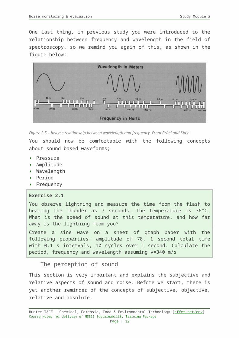
One last thing, in previous study you were introduced to the relationship between frequency and wavelength in the field of spectroscopy, so we remind you again of this, as shown in the figure below;

Figure 2.5 – Inverse relationship between wavelength and frequency. From Brüel and Kjær.

You should now be comfortable with the following concepts about sound based waveforms;

◗ Pressure◗ Amplitude◗ Wavelength◗ Period◗ Frequency

Exercise 2.1

You observe lightning and measure the time from the flash to hearing the thunder as 7 seconds. The temperature is 36°C. What is the speed of sound at this temperature, and how far away is the lightning from you?

Create a sine wave on a sheet of graph paper with the following properties: amplitude of 78, 1 second total time with 0.1 s intervals, 10 cycles over 1 second. Calculate the period, frequency and wavelength assuming v=340 m/s



The perception of soundThis section is very important and explains the subjective and relative aspects of sound and noise. Before we start, there is yet another reminder of the concepts of subjective, objective, relative and absolute.

Subjective exists in your mind and belongs to the thinking subject, you. It is when something is characteristic of the individual, and could depend upon such things as your mood or attitude. Loosely, it is ‘in your opinion’.

Objective is the opposite of subjective and involves measuring against factual evidence where personal feelings or attitudes are not influencing the outcome as they are the object of perception and thought rather than being the object of emotion.

Relative refers to the subjects being considered (or measured) against something else by being made ‘relative’ to each other and not being independent. Relative humidity is the current humidity when compared to the current potential for saturation (≥100% humidity).

Absolute is the opposite of relative and is free from restriction or condition, which, in the humidity example, would be vapour pressure (as an absolute measure of moisture).

Subjective versus objective

Sound pressure levels are highly objective and are measured by microphones (which are a type of transducer, as is the human ear) and are reported on a decibel scale (The higher the decibels, the louder the sound - discussed later). Loudness however, is a subjective quantity – and must therefore be measured by a scale that is subjective and requires human judgement.

The subjective response to the absolute sound pressure level is referred to as loudness which is measured in a unit called the phon. Because one phon is equal to the perceived loudness of a 1 dB sound at 1,000Hz, loudness is frequency dependent, as the human ear is more sensitive to some frequencies than others.

The subjective analysis of frequency (which itself is objective) is called pitch. You may have read or heard “a high pitch scream”. This would imply that the sound was of a high frequency, but relative to what? It is usually relative to standard human speech (~ 1000 to 4000 Hz), therefore any vocal activity above 4000 Hz is of high pitch, subjectively.

Loudness, phons & sonesSo, loudness is the subjective sound quality that is the human equivalent of amplitude, or for want of a better term, the volume. We need to quantify loudness because the human hearing mechanisms does not correlate with sound pressure equally over all frequencies, or all amplitudes, so what we think is 80 decibels at 1000 Hz only sounds like 68 decibels at 100 Hz.



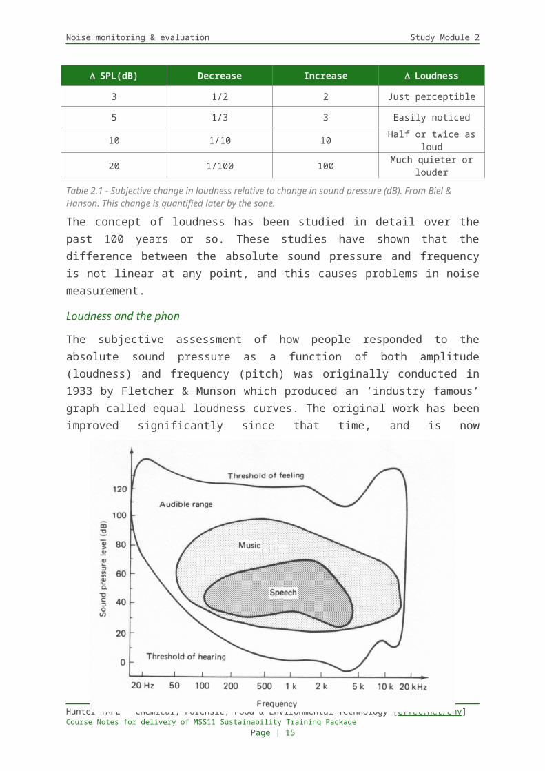
SPL(dB) Decrease Increase Loudness

3 1/2 2 Just perceptible

5 1/3 3 Easily noticed

10 1/10 10 Half or twice as loud

20 1/100 100 Much quieter or louder

Table 2.1 - Subjective change in loudness relative to change in sound pressure (dB). From Biel & Hanson. This change is quantified later by the sone.

The concept of loudness has been studied in detail over the past 100 years or so. These studies have shown that the difference between the absolute sound pressure and frequency is not linear at any point, and this causes problems in noise measurement.

Loudness and the phon

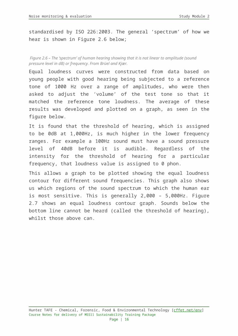
The subjective assessment of how people responded to the absolute sound pressure as a function of both amplitude (loudness) and frequency (pitch) was originally conducted in 1933 by Fletcher & Munson which produced an ‘industry famous’ graph called equal loudness curves. The original work has been improved significantly since that time, and is now standardised by ISO 226:2003. The general ‘spectrum’ of how we hear is shown in Figure 2.6 below;



Figure 2.6 – The ‘spectrum’ of human hearing showing that it is not linear to amplitude (sound pressure level in dB) or frequency. From Brüel and Kjær.

Equal loudness curves were constructed from data based on young people with good hearing being subjected to a reference tone of 1000 Hz over a range of amplitudes, who were then asked to adjust the ‘volume’ of the test tone so that it matched the reference tone loudness. The average of these results was developed and plotted on a graph, as seen in the figure below.

It is found that the threshold of hearing, which is assigned to be 0dB at 1,000Hz, is much higher in the lower frequency ranges. For example a 100Hz sound must have a sound pressure level of 40dB before it is audible. Regardless of the intensity for the threshold of hearing for a particular frequency, that loudness value is assigned to 0 phon.

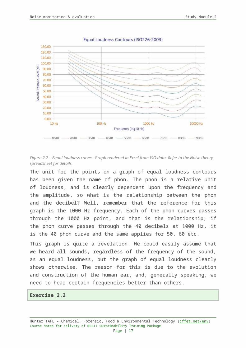
This allows a graph to be plotted showing the equal loudness contour for different sound frequencies. This graph also shows us which regions of the sound spectrum to which the human ear is most sensitive. This is generally 2,000 – 5,000Hz. Figure 2.7 shows an equal loudness contour graph. Sounds below the bottom line cannot be heard (called the threshold of hearing), whilst those above can.

Figure 2.7 – Equal loudness curves. Graph rendered in Excel from ISO data. Refer to the Noise theory spreadsheet for details.

The unit for the points on a graph of equal loudness contours has been given the name of phon. The phon is a relative unit of loudness, and is clearly dependent upon the frequency and the amplitude, so what is the relationship between the phon and the decibel? Well, remember that the reference for this graph is the 1000 Hz frequency. Each of the phon curves passes through the 1000 Hz point, and that is the relationship; if the phon curve



passes through the 40 decibels at 1000 Hz, it is the 40 phon curve and the same applies for 50, 60 etc.

This graph is quite a revelation. We could easily assume that we heard all sounds, regardless of the frequency of the sound, as an equal loudness, but the graph of equal loudness clearly shows otherwise. The reason for this is due to the evolution and construction of the human ear, and, generally speaking, we need to hear certain frequencies better than others.

Exercise 2.2

There is a physiological importance to the fact that we hear best at certain frequencies. Discuss why this may be the case (hint: it is related to the vocal chords).

Loudness and the sone

But how do we describe the relative loudness between two phon curves? Sadly the graph doesn’t tell us anything about the relative loudness of phons. Above it was discussed that a change in 3 dB was considered ‘just audible’, whereas a change in 10 dB was considered to be ‘half or twice’ as loud.

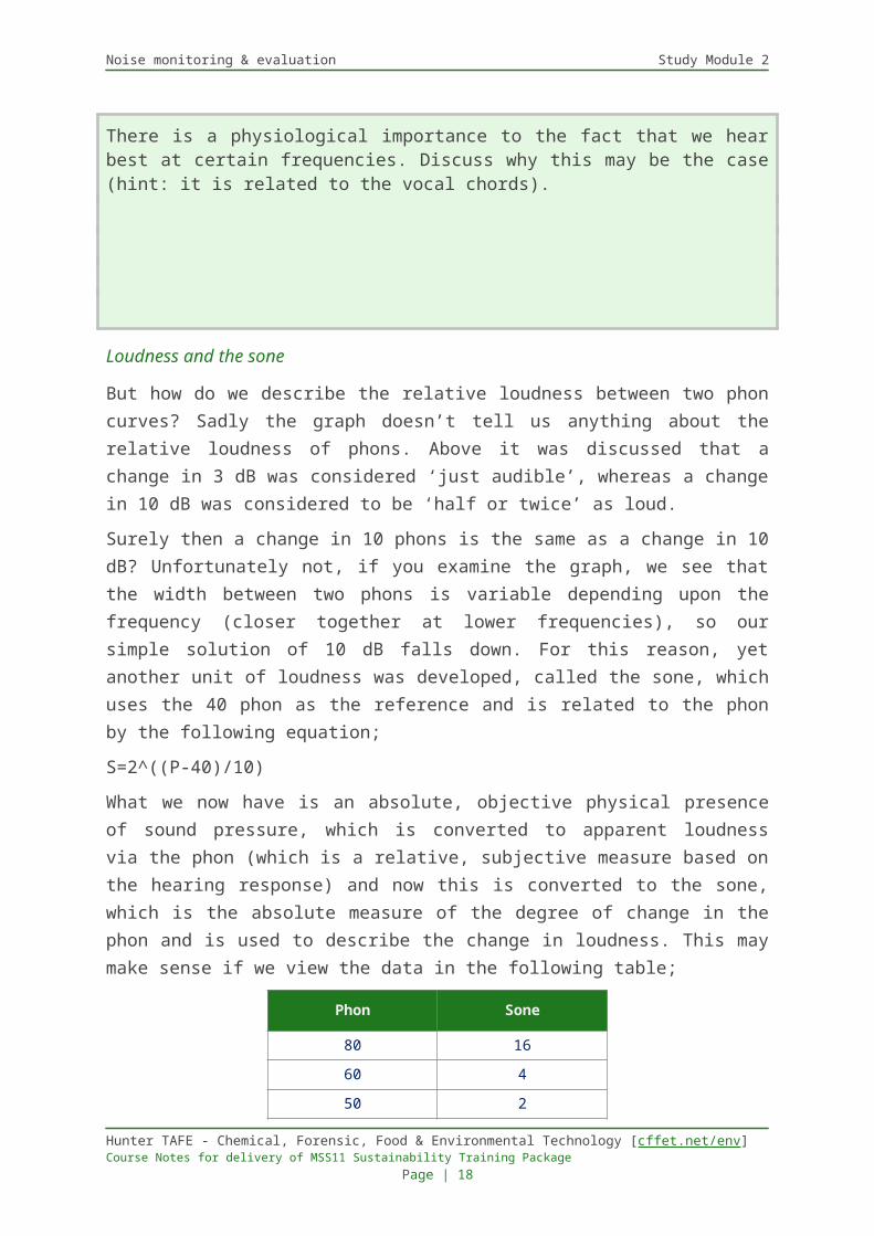
Surely then a change in 10 phons is the same as a change in 10 dB? Unfortunately not, if you examine the graph, we see that the width between two phons is variable depending upon the frequency (closer together at lower frequencies), so our simple solution of 10 dB falls down. For this reason, yet another unit of loudness was developed, called the sone, which uses the 40 phon as the reference and is related to the phon by the following equation;

S=2^((P-40)/10)

What we now have is an absolute, objective physical presence of sound pressure, which is converted to apparent loudness via the phon (which is a relative, subjective measure based on the hearing response) and now this is converted to the sone, which is the absolute measure of the degree of change in the phon and is used to describe the change in loudness. This may make sense if we view the data in the following table;

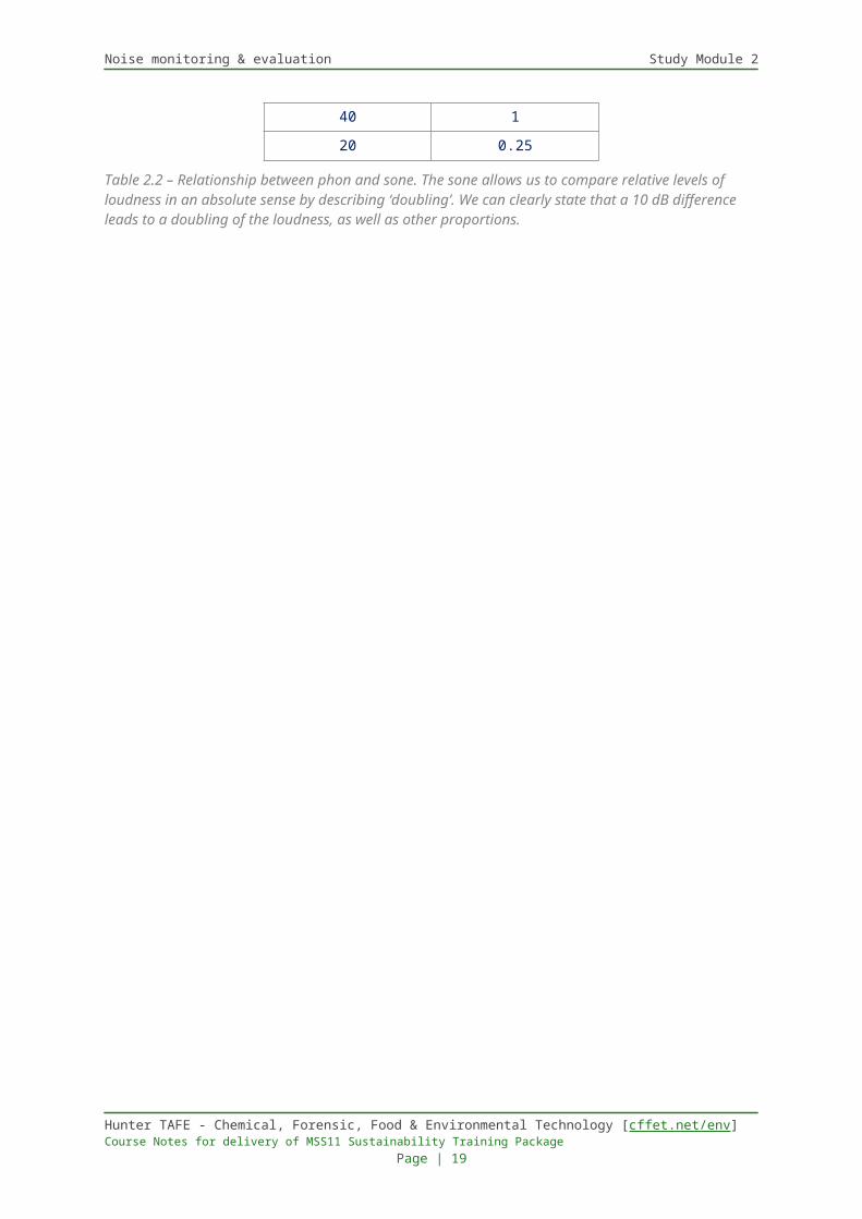
Phon Sone

80 16

60 4

50 2

40 1

20 0.25



Table 2.2 – Relationship between phon and sone. The sone allows us to compare relative levels of loudness in an absolute sense by describing ‘doubling’. We can clearly state that a 10 dB difference leads to a doubling of the loudness, as well as other proportions.



Summary

So, this chapter brings together all the important aspects of sound so that you can get an understanding of the problems associated with how to measure it. A summary of the key points is outlined below.

◗ Sound pressure exists as waves which have unique properties that allow us to define the waves, the really important ones are amplitude and frequency.

◗ The amplitude is governed by the power creating the sound pressure (which is a lot smaller in magnitude than atmospheric pressure).

◗ A pure tone has one frequency, noise has hundreds or thousands, all of which can be determined by the Fast Fourier Transform inside the noise meter.

◗ How we hear these sounds is very different to the absolute sound pressure hitting our ears, due to the subjective response by our brain, and is referred to as loudness.

◗ The difference between the absolute sound pressure (amplitude) and what we hear (loudness) is related by the relative unit called the phon.

◗ The change in relative loudness can be quantitatively described by the sone.◗ This knowledge is required to understand how noise meters work.



Assessment task

After reading the theory above, answer the questions below. Note that;

Marks are allocated to each question.

Keep answers to short paragraphs only, no essays.

Make sure you have access to the references (last page)

If a question is not referenced, use the supplied notes for answers

Complete the following table of terms and definitions. 0 mkTerm Definition

Sound Type your answer here

Pressure Type your answer here

Pascal Type your answer here

Amplitude Type your answer here

Magnitude Type your answer here

Compression Type your answer here

Rarefaction Type your answer here

Transverse Type your answer here

Longitudinal Type your answer here

Wavelength Type your answer here

Period Type your answer here

Frequency Type your answer here

Velocity Type your answer here

Speed of sound Type your answer here

Subjective Type your answer here

Objective Type your answer here

Relative Type your answer here



Absolute Type your answer here

Loudness Type your answer here

Equal loudness curves Type your answer here

Phon Type your answer here

Sone Type your answer here

Answer the following questions1. What is the difference between a sound and a pressure wave? 2 mk

Type your answer here

Leave blank for assessor feedback

2. How is a sound wave generated? 5 mk



3. What is the difference between compression and rarefaction? 4 mk

Type you answer here


4. Provide an example or definition that outlines the key differences between a transverse and a longitudinal wave. 4 mk





5. Describe how the human ear perceives a change in amplitude? 2 mk



6. Describe the relationship between frequency and wavelength. 4 mk



7. What is the difference between period and frequency? 2 mk



8. By what mathematical technique are the frequencies of complex signals determined? 2 mk



9. What is the subjective response to amplitude called? 1 mk



10. What is the subjective response to frequency called? 1 mk





11. What is the unit for loudness? 1 mk



12. Describe how loudness differs to the absolute sound pressure. 6 mk



13. What does the sone tell us about loudness? 4 mk





Assessment & submission rules

Answers◗ Attempt all questions and tasks◗ Write answers in the text-fields provided

Submission◗ Use the documents ‘Save As…’ function to save the document to your computer using

the file name format of;name-classcode-assessmentname

Note that class code and assessment code are on Page 1 of this document.

◗ email the document back to your teacher

Penalties◗ If this assessment task is received greater than seven (7) days after the due date (located

on the cover page), it may not be considered for marking without justification.

Results◗ Your submitted work will be returned to you within 3 weeks of submission by email fully

graded with feedback.◗ You have the right to appeal your results within 3 weeks of receipt of the marked work.

Problems?If you are having study related or technical problems with this document, make sure you contact your assessor at the earliest convenience to get the problem resolved. The name of your assessor is located on Page 1, and the contact details can be found at;

www.cffet.net/env/contacts

Resources & referencesReferences

(NSW), E. P. (2000). NSW Industrial Noise Policy. Sydney: Environmental Protection Authority (NSW).

(NSW), R. &. (2001). Environmental Noise Management Manual. Sydney: Roads & Traffic Authority (NSW).

Australia, S. (1997). AS 1055.1-3. Homebush: Standards Australia.

Australia, S. (2005). OCcupational Noise Management, Part 1: Measurement and Assessment of Noise Immission and Exposure. Homebush: Standards Australia.

Australia, S. (2011). Methods for the sampling & analysis of ambient air: Part 14: Meteorological monitoring for ambient air quality monitoring applications. Homebush: Standards Australia.

Bies, D. &. (2003). Engineering Noise Control, 3rd Ed. London: Spon Press.

Kester, W. (2004). Analogue-Digital Conversion. United States: Analogue Devices.


http://www.cffet.net/env/contacts


Maltby. (2005). Occupational Audiometry: Monitoring & protecting hearing at work. London: Elselvier.

NOHSC. (2000). National Standard for Occupational Noise [NOHSC: 1007(2000), 2nd Ed. Canberra: Australian Government.

Organisation, W. H. (1995). Occupational Exposure to noise: Evaluation, prevention & control. Geneva: WHO Publishing.

Rossing, T. (2007). Handbook of Acoustics. New York: Springer.

South, T. (2004). Managin Noise & Vibration at Work. London: Elselvier.

Workcover, N. (2004). Code of Practice: Noise Management & Protection of Hearing at Work. Sydney: Workcover NSW.

Workplace Health and Safety Regulation 2011. (n.d.).

Further reading and online aids

Nil


Documents

Navigation Techniques for Environmental Technicians · Web viewEnvironmental Monitoring & Technology Series Noise monitoring & evaluation For Technicians Study module 2 Introduction