NBER WORKING PAPER SERIES

AUTOMATIC STABILIZERS AND ECONOMIC CRISIS: US VS. EUROPE

Mathias DollsClemens FuestAndreas Peichl

Working Paper 16275http://www.nber.org/papers/w16275

NATIONAL BUREAU OF ECONOMIC RESEARCH1050 Massachusetts Avenue

Cambridge, MA 02138August 2010

This paper uses EUROMOD version D21 and TAXSIM v9. EUROMOD and TAXSIM arecontinually being improved and updated and the results presented here represent the best availableat the time of writing. Our version of TAXSIM is based on the Survey of Consumer Finances (SCF)by the Federal Reserve Board. EUROMOD relies on micro-data from 17 different sources for 19countries. These are ECHP and EU-SILC (Eurostat), Austrian version of ECHP (Statistik Austria);PSBH (University of Liège and University of Antwerp); Estonian HBS (Statistics Estonia); IncomeDistribution Survey (Statistics Finland); EBF (INSEE); GSOEP (DIW Berlin); Greek HBS (NationalStatistical Service of Greece); Living in Ireland Survey (ESRI); SHIW (Bank of Italy); PSELL-2(CEPS/INSTEAD); SEP (Statistics Netherlands); Polish HBS (Warsaw University); Slovenian HBSand Personal Income Tax database (Statistical Office of Slovenia); Income Distribution Survey(Statistics Sweden); and the FES (UK ONS through the Data Archive). Material from the FES isCrown Copyright and is used by permission. Neither the ONS nor the Data Archive bears anyresponsibility for the analysis or interpretation of the data reported here. An equivalent disclaimerapplies for all other data sources and their respective providers. This paper is partly based on work

carried out during Andreas Peichl's visit to ECASS at ISER, University of Essex, supported by theEU Improving Human Potential Programme. Andreas Peichl is grateful for financial support byDeutsche Forschungsgemeinschaft DFG (PE1675). Clemens Fuest acknowledges financial supportfrom the ESRC (Grant No RES-060-25-0033). We would like to thank Danny Blanchflower, DeanBaker, Horacio Levy, Torfinn Harding, Tommaso Monacelli, Morten Ravn, participants of the 2009IZA/CEPR ESSLE conference, the 6th German-Norwegian Seminar on Public Economics (CESifo),the 2010 IZA/OECD workshop, the NBER/IGIER TAPES meeting as well as seminar participantsin Bonn, Cologne, Nuremberg, Siegen and at the Worldbank for helpful comments and suggestions.We are grateful to Daniel Feenberg for granting us access to NBER's TAXSIM and helping us withour simulations. We are indebted to all past and current members of the EUROMOD consortium forthe construction and development of EUROMOD. The usual disclaimer applies. The viewsexpressed herein are those of the authors and do not necessarily reflect the views of the NationalBureau of Economic Research.

© 2010 by Mathias Dolls, Clemens Fuest, and Andreas Peichl. All rights reserved. Short sectionsof text, not to exceed two paragraphs, may be quoted without explicit permission provided that fullcredit, including © notice, is given to the source.

Automatic Stabilizers and Economic Crisis: US vs. EuropeMathias Dolls, Clemens Fuest, and Andreas PeichlNBER Working Paper No. 16275August 2010JEL No. E32,H2,H31

ABSTRACT

This paper analyzes the effectiveness of the tax and transfer systems in the European Union and theUS to act as an automatic stabilizer in the current economic crisis. We find that automatic stabilizersabsorb 38 per cent of a proportional income shock in the EU, compared to 32 per cent in the US. Inthe case of an unemployment shock 47 percent of the shock are absorbed in the EU, compared to 34per cent in the US. This cushioning of disposable income leads to a demand stabilization of up to 30per cent in the EU and up to 20 per cent in the US. There is large heterogeneity within the EU. Automaticstabilizers in Eastern and Southern Europe are much lower than in Central and Northern Europeancountries. We also investigate whether countries with weak automatic stabilizers have enacted largerfiscal stimulus programs. We find no evidence supporting this view.

Mathias DollsUniversity of CologneCologne Graduate School in Management, Economics and Social Sciences Richard-Strauß-Str. 250931 CologneGermanydolls@wiso.uni-koeln.de

Clemens FuestSaïd Business SchoolUniversity of OxfordPark End StreetOxfordOX1 1HPUKClemens.Fuest@sbs.ox.ac.uk

Andreas PeichlIZA - Institute for the Study of LaborSchaumburg-Lippe-Str. 5-9,53113 Bonn, Germanypeichl@iza.org

1 Introduction

In the current economic crisis, the workings of automatic stabilizers are widely seen

to play a key role in stabilizing demand and output. Automatic stabilizers are usu-

ally de�ned as those elements of �scal policy which mitigate output �uctuations

without discretionary government action (see, e.g., Eaton and Rosen (1980)). De-

spite the importance of automatic stabilizers for stabilizing the economy, �very little

work has been done on automatic stabilization [...] in the last 20 years� (Blan-

chard (2006)). However, especially in the current crisis, it is important to assess

the contribution of automatic stabilizers to overall �scal expansion and to compare

their magnitude across countries. Previous research on automatic stabilization has

mainly relied on macro data. Exceptions based on micro data are Auerbach and

Feenberg (2000) for the US and Mabbett and Schelkle (2007) for the EU-15. More

comparative work based on micro data has been conducted on the di¤erences in the

tax wedge and e¤ective marginal tax rates between the US and European countries

(see, e.g., Piketty and Saez (2007)).

In this paper, we combine these two strands of the literature to compare the

magnitude and composition of automatic stabilization between the US and Europe

based on micro data estimates. We analyze the impact of automatic stabilizers

using microsimulation models for 19 European countries (EUROMOD) and the US

(TAXSIM). The microsimulation approach allows us to investigate the causal e¤ects

of di¤erent types of shocks on household disposable income, holding everything else

constant (see Bourguignon and Spadaro (2006)). Thus we can single out the role

of automatic stabilization. This is much more di¢ cult in an ex-post evaluation (or

with macro level data) as it is not possible to disentangle the e¤ects of automatic

stabilizers, active �scal and monetary policy and behavioral responses like changes

in labor supply or disability bene�t take-up in such a framework. Our simulation

analysis therefore complements the macro literature on the relationship between gov-

ernment size and volatility (e.g., Galí (1994), Fatàs and Mihov (2001)) by providing

estimates for the size of automatic stabilizers.

We run two controlled experiments of macro shocks to income and employment.

The �rst is a proportional decline in household gross income by 5% (income shock).

This is the usual way of modeling aggregate shocks in simulation studies analyz-

ing automatic stabilizers. However, economic downturns typically a¤ect households

asymmetrically, with some households losing their jobs and su¤ering a sharp decline

1

in income and other households being much less a¤ected, as wages are usually rigid

in the short term. We therefore consider a second idiosyncratic shock where some

households become unemployed, so that the unemployment rate increases such that

total household income decreases by 5% (unemployment shock). This idiosyncratic

shock a¤ects each household in a di¤erent way with income losses ranging between

zero (if the household is not a¤ected) and total household gross income (in case all

members of the household become unemployed). We show that these two types of

shocks and the resulting stabilization coe¢ cients can be interpreted as an average

e¤ective marginal tax rate (EMTR) for the whole tax bene�t system at the inten-

sive (proportional income shock) or extensive (unemployment shock) margin. After

identifying the e¤ects of these shocks on disposable income, we use various methods

to estimate the prevalence of credit constraints among households. Among these is

the approach by Zeldes (1989) where �nancial wealth is the determinant for credit

constraints, but also alternative approaches which are based on information regard-

ing home ownership (Runkle (1991)) as well as on direct survey evidence (Jappelli

et al. (1998)). On this basis, we calculate how the stabilization of disposable income

can translate into demand stabilization.

As our measure of automatic stabilization, we extend the normalized tax change

(Auerbach and Feenberg (2000)) to include other taxes as well as social contributions

and bene�ts. Our income stabilization coe¢ cient relates the shock absorption of

the whole tax and transfer system to the overall size of the income shock. We

take into account personal income taxes (at all government levels), social insurance

contributions and payroll taxes paid by employers and employees, value added or

sales taxes as well as transfers to private households such as unemployment bene�ts.1

Computations are done according to the tax bene�t rules which were in force before

2008 in order to avoid an endogeneity problem resulting from policy responses after

the start of the crisis.

What does the present paper contribute to the literature? First, previous studies

have focused on proportional income shocks whereas our analysis shows that auto-

matic stabilizers work very di¤erently in the case of unemployment shocks, which

a¤ect households asymmetrically.2 This is especially important for assessing the ef-

1We abstract from other taxes, in particular corporate income taxes. For an analysis of au-tomatic stabilizers in the corporate tax system see Devereux and Fuest (2009) and Buettner andFuest (forthcoming).

2Auerbach and Feenberg (2000) do consider a shock where households at di¤erent incomelevels are a¤ected di¤erently, but the results are very similar to the case of a symmetric shock.

2

fectiveness of automatic stabilizers in the current economic crisis. Second, we extend

the micro data measure on automatic stabilization to di¤erent taxes and bene�ts.

Our analysis includes a decomposition of the overall stabilization e¤ects into the

contributions of taxes, social insurance contributions and bene�ts. A further dif-

ference between our study and Auerbach and Feenberg (2000) is that we take into

account unemployment bene�ts and state level income taxes. This explains why our

estimates of overall automatic stabilization e¤ects in the US are higher. In two ex-

tensions, we also consider consumption taxes and employer�s contributions. Third,

to the best of our knowledge, our study is the �rst to estimate the prevalence of

liquidity constraints for such a large set of European countries based on household

data.3 This is of key importance for assessing the role of automatic stabilizers for

demand smoothing. Moreover, we use several di¤erent strategies for estimating liq-

uidity constraints in order to explore the sensitivity of demand stabilization results.

Fourth, we extend the analysis to more recent years and countries - including tran-

sition countries from Eastern Europe - and we compare the US and Europe within

the same microeconometric framework. Finally, we shed light on the issue whether

macro indicators are a good proxy for micro data based stabilization coe¢ cients. We

also investigate whether bigger governments or more open economies have higher or

lower automatic stabilizers.

We show that our extensions to previous research are important for the com-

parison between the U.S. and Europe as they help to identify driving forces in

automatic stabilization. Our analysis leads to the following main results. In the

case of an income shock, approximately 38% of the shock would be absorbed by

automatic stabilizers in the EU. For the US, we �nd a value of 32%. This is surpris-

ing because automatic stabilizers in Europe are usually perceived to be drastically

higher than in the US. Our results qualify this view to some extent, at least as far

as proportional macro shocks on household income are concerned. When looking at

the personal income tax only, the values for the US are even higher than the EU

average. Within the EU, there is considerable heterogeneity, and results for overall

stabilization of disposable income range from a value of 25% for Estonia to 56%

for Denmark. In general, automatic stabilizers in Eastern and Southern European

Our analysis con�rms this for the US, but not for Europe.3There are several studies on liquidity constraints and the responsiveness of households to tax

changes for the US (see, e.g., Zeldes (1989), Parker (1999), Souleles (1999), Johnson et al. (2006),Shapiro and Slemrod (1995, 2003, 2009))

3

countries are considerably lower than in Continental and Northern European coun-

tries. In the case of the idiosyncratic unemployment shock, the di¤erence between

the EU and the US is larger. EU automatic stabilizers absorb 47% of the shock

whereas the stabilization e¤ect in the US is only 34%. Again, there is considerable

heterogeneity within the EU.

How does this cushioning of shocks translate into demand stabilization? If de-

mand stabilization can only be achieved for liquidity constrained households, the

picture changes signi�cantly. Here, the results are sensitive with respect to the

method used for estimating liquidity constraints. For the income shock, the cush-

ioning e¤ect of automatic stabilizers is now in the range of 4-22% in the EU and

between 6-17% in the US. For the unemployment shock, however, we �nd a larger

di¤erence. In the EU, the stabilization e¤ect substantially exceeds the comparable

US value for all liquidity constraint estimation methods. It ranges from 13-30%

whereas results for the US are between 7-20% and are similar to the values for the

income shock. These results suggest that social transfers, in particular the rather

generous systems of unemployment insurance in Europe, play a key role for demand

stabilization and explain an important part of the di¤erence in automatic stabilizers

between Europe and the US.

A �nal issue we discuss in the paper is how �scal stimulus programs of individual

countries are related to automatic stabilizers. In particular, we ask whether countries

with low automatic stabilizers have tried to compensate this by larger �scal stimuli,

but we �nd no correlation between the size of �scal stimulus programs and automatic

stabilizers. However, we do �nd that discretionary �scal policy programmes have

been smaller in more open economies.

The paper is structured as follows. In Section 2 we provide a short overview

of previous research with respect to automatic stabilization and comparisons of US

and European tax bene�t systems. In addition, we discuss how stabilization e¤ects

can be measured. Section 3 describes the microsimulation models EUROMOD and

TAXSIM and the di¤erent macro shock scenarios we consider. Section 4 presents

the results on automatic stabilization which are discussed in Section 5 together with

potential limitations of our approach. Section 6 concludes.

4

2 Previous research and theoretical framework

2.1 Previous research

There are two strands of literature which are related to our paper. The �rst is the

literature on the analysis and measurement of automatic �scal stabilizers. In the

empirical literature4, two types of studies prevail: macro data studies and micro

data approaches.5 The common baseline of macro data studies is to measure the

cyclical elasticitiy of di¤erent budget components such as the income tax, social

security contributions, the corporate tax, indirect taxes or unemployment bene�ts.

Di¤erent approaches have been proposed, for example regressing changes in �scal

variables on the growth rate of GDP or estimating elasticities on the basis of macro-

econometric models.6 Sachs and Sala-i Martin (1992) and Bayoumi and Masson

(1995) use time series data and �nd values of 30%-40% for disposable income stabi-

lization in the US. However, these approaches raise several issues, in particular the

challenge of separating discretionary actions from automatic stabilizers in combina-

tion with identi�cation problems resulting from endogenous regressors. Related to

the literature on macro estimations of automatic stabilization are studies that focus

on the relationship between output volatility, public sector size and openness of the

economy (Cameron (1978), Galí (1994), Rodrik (1998), Fatàs and Mihov (2001),

Auerbach and Hassett (2002)).

Much less work has been done on the measurement of automatic stabilizers

with micro data. Auerbach and Feenberg (2000) use the NBER�s microsimulation

model TAXSIM to estimate the automatic stabilization for the US from 1962-954A theoretical analysis of automatic stabilizers in a real business cycle (RBC) model can be

found in Galí (1994). One issue of standard RBC models is that they are not able to explainthe stylized fact that the size of government (as a proxy for automatic stabilizers) is negativelycorrelated with the volatility of business cycles. In fact, under some reasonable assumptions, astandard RBC model produces a positive correlation (Andrés et al. (2008)). In addition, suchmodels are not able to explain evidence that consumption responds positively to increases ingovernment spending (Blanchard and Perotti (2002), Fatàs and Mihov (2002) or Perotti (2002)).These facts, however, can be easily explained by a simple textbook IS-LM model as well as bylarge-scale macroeconometric models (van den Noord (2000), Buti and van den Noord (2004)).Galí et al. (2007) and Andrés et al. (2008) show that both facts can only be explained in a RBCmodel by adding Keynesian features like nominal and real rigidities in combination with rule-of-thumb consumers to the analysis.

5Early estimates on the responsiveness of the tax system to income �uctuations are discussedin the Appendix of Goode (1976). More recent contributions include Fatàs and Mihov (2001),Blanchard and Perotti (2002), Mélitz and Zumer (2002).

6Cf. van den Noord (2000) or Girouard and André (2005).

5

and �nd values for the stabilization of disposable income ranging between 25%-35%.

Auerbach (2009) has updated this analysis and �nds a value of around 25% for more

recent years. Mabbett and Schelkle (2007) conduct a similar analysis for 15 Western

European countries in 1998 and �nd higher stabilization e¤ects than in the US, with

results ranging from 32%-58%.7 How does this smoothing of disposable income a¤ect

household demand? To the best of our knowledge, Auerbach and Feenberg (2000)

is the only simulation study which estimates the demand e¤ect taking into account

liquidity constraints. They use the method suggested by Zeldes (1989) and �nd

that approximately two thirds of all households are likely to be liquidity constrained.

Given this, the contribution of automatic stabilizers to demand smoothing is reduced

to approximately 15% of the initial income shock.

The second strand of related literature focuses on international comparisons of

income tax systems in terms of e¤ective average and marginal tax rates, and in-

dividual tax wedges between the US and European countries. This literature has

mainly relied on micro data and the simulation approach in order to take into ac-

count the heterogeneity of the population. Piketty and Saez (2007) use a large

public micro-�le tax return data set for the US to compute average tax rates for �ve

federal taxes and di¤erent income groups. They complement the analysis for the

US with a comparison to France and the UK. A key �nding from their analysis is

that today (and in contrast to 1970), France, a typical continental European welfare

state, has higher average tax rates than the two Anglo-Saxon countries. The French

tax system is also more progressive. Immvervoll (2004) discusses conceptual issues

with regard to macro- and micro-based measures of the tax burden and compares

e¤ective tax rates in fourteen EU Member States. In general, he �nds a large hetero-

geneity across countries with average and marginal e¤ective tax rates being lowest

in southern European countries. Other studies take as given that European tax

systems reveal a higher degree of progressivity (e.g. Alesina and Glaeser (2004)) or

higher (marginal) tax rates in general (e.g. Prescott (2004) or Alesina et al. (2005))

and discuss to what extent di¤erences in economic outcomes such as hours worked

can be explained by di¤erent tax structures. By providing new measures of the aver-

age e¤ective marginal tax rate (EMTR) both at the intensive and extensive margin

7Mabbett and Schelkle (2007) rely for their analysis (which is a more recent version of Mabbett(2004)) on the results from an in�ation scenario taken from Immvervoll et al. (2006) who use themicrosimulation model EUROMOD to increase earnings by 10% in order to simulate the sensitivityof poverty indicators with respect to macro level changes.

6

for the US and 19 European countries, this paper sheds further light on existing

di¤erences between the US and European tax and transfer systems.

2.2 Theoretical framework

The extent to which automatic stabilizers mitigate the impact of income shocks on

household demand essentially depends on two factors. First, the tax and transfer

system determines the way in which a given shock to gross income translates into a

change in disposable income. For instance, in the presence of a proportional income

tax with a tax rate of 40%, a shock on gross income of one hundred Euros leads

to a decline in disposable income of 60 Euros. In this case, the tax absorbs 40%

of the shock to gross income. A progressive tax, in turn, would have a stronger

stabilizing e¤ect. The second factor is the link between current disposable income

and current demand for goods and services. If the income shock is perceived as

transitory and current demand depends on some concept of permanent income, and

if households can borrow or use accumulated savings, their demand will not change.

In this case, the impact of automatic stabilizers on current demand would be equal

to zero. Things are di¤erent, though, if some households are liquidity constrained

or acting as �rule-of-thumb� consumers (Campbell and Mankiw (1989)). In this

case, their current expenditures do depend on disposable income so that automatic

stabilizers play a role.

A common measure for estimating automatic stabilization is the �normalized tax

change�used by Auerbach and Feenberg (2000) which can be interpreted as �the

tax system�s built-in �exibility�(Pechman (1973, 1987)). It shows how changes in

market income translate into changes in disposable income through changes in per-

sonal income tax payments. We extend the concept of normalized tax change to

include other taxes as well as social insurance contributions and transfers like e.g.

unemployment bene�ts. We take into account personal income taxes (at all govern-

ment levels), social insurance contributions as well as payroll taxes and transfers to

private households such as unemployment bene�ts.

Market income Y Mi of individual i is de�ned as the sum of all incomes from

market activities:

Y Mi = Ei +Qi + Ii + Pi +Oi (1)

where Ei is labour income, Qi business income, Ii capital income, Pi property in-

7

come, and Oi other income. Disposable income Y Di is de�ned as market income

minus net government intervention Gi = Ti + Si �Bi :

Y Di = Y Mi �Gi = Y Mi � (Ti + Si �Bi) (2)

where Ti are direct taxes, Si employee social insurance contributions, and Bi are

social cash bene�ts (i.e. negative taxes). Note that an extended analysis includ-

ing employer social insurance contributions and consumption taxes is presented in

Section 4.4.

We analyze the impact of automatic stabilizers in two steps. The �rst is the

stabilization of disposable income and the second is the stabilization of demand.

Consider �rst the stabilization of disposable income. Throughout the rest of the

paper, we refer to our measure of this e¤ect as the income stabilization coe¢ cient

� I . We derive � I from a general functional relationship between disposable income

and market income:

� I = � I(Y M ; T; S;B): (3)

The derivation can be either done at the macro or at the micro level. On the

macro level, the aggregate change in market income (�Y M) is transmitted via � I

into an aggregate change in disposable income (�Y D):

�Y D = (1� �)�Y M (4)

However, one issue when computing � I based on the change of macro level aggr-

gates is that macro data changes include behavioral and general equilibrium e¤ects

as well as discretionary policy measures. Therefore, a measure of automatic sta-

bilization based on macro data changes captures all these e¤ects. Thus, it is not

possible to disentangle the automatic stabilization from stabilization through dis-

cretionary policies or changes in behavior because of endogeneity and identi�cation

problems. That is why in these studies the correlation between government size

and output volatility is analyzed as a proxy for automatic stabilization. To com-

plement this literature and in order to isolate the impact of automatic stabilization

from other e¤ects, we compute � I using arithmetic changes (�) in total disposable

income (P

i�YDi ) and market income (

Pi�Y

Mi ) based on micro data information

taken from a microsimulation tax-bene�t calculator, which - by de�nition - avoids

endogeneity problems by simulating exogenous changes (Bourguignon and Spadaro

8

(2006))8:

Xi

�Y Di = (1� � I)Xi

�Y Mi

� I = 1�P

i�YDiP

i�YMi

=

Pi

��Y Mi ��Y Di

�Pi�Y

Mi

=

Pi�GiPi�Y

Mi

(5)

where � I measures the sensitivity of disposable income, Y Di ; with respect to market

income, Y Mi . The higher �I , the stronger the stabilization e¤ect. For example,.

� I = 0:4 implies that 40% of the income shock is absorbed by the tax bene�t

system. Note that the income stabilization coe¢ cient is not only determined by the

size of government (e.g. measured as expenditure or revenue in percent of GDP)

but also depends on the structure of the tax bene�t system and the design of the

di¤erent components.

The de�nition of � I resembles that of an average e¤ective marginal tax rate

(EMTR), which is usually computed in this way using micro data (Immvervoll

(2004)). In the case of the proportional income shock, � I can be interpreted as

the EMTR along the intensive margin, whereas in the case of the unemployment

shock, it resembles the EMTR along the extensive margin (participation tax rate,

see, e.g., Saez (2001, 2002), Kleven and Kreiner (2006) or Immervoll et al. (2007)).

Another advantage of the micro data based approach is that it enables us to ex-

plore the extent to which di¤erent individual components of the tax transfer system

contribute to automatic stabilization. Comparing tax bene�t systems in Europe

and the US, we are interested in the weight of each component in the respective

country. We therefore decompose the coe¢ cient into its components which include

taxes, social insurance contributions and bene�ts:

� I =Xf

� If = �IT+�

IS+�

IB =

Pi�TiPi�Y

Mi

+

Pi�SiPi�Y

Mi

�P

i�BiPi�Y

Mi

=

Pi (�Ti +�Si ��Bi)P

i�YMi

(6)

Consider next the second step of the analysis, the impact on demand. In order to

8Note that a potential drawback of this approach is that we neglect general equilibrium e¤ectsas well as behavioral adjustments as a response to an income shock. This, however, is done onpurpose, as we do not aim at quantifying the overall adjustment to a shock but to single out thesize of automatic stabilizers, which - by de�nition - automatically smooth incomes without takinginto account the e¤ects of discretionary policy action or behavioral responses.

9

stabilize �nal demand and output, the cushioning e¤ect on disposable income has to

be transmitted to expenditures for goods and services. If current demand depends

on some concept of permanent income, demand will not change in response to a

transitory income shock. Things are di¤erent, though, if households are liquidity

constrained and cannot borrow. In this case, their current expenditures do depend

on disposable income so that automatic stabilizers play a role. Following Auerbach

and Feenberg (2000), we assume that households who face liquidity constraints fully

adjust consumption expenditure after changes in disposable income while no such

behavior occurs among households without liquidity constraints.9 The adjustment of

liquidity constrained households is such that changes in disposable income are equal

to changes in consumption. Hence, the coe¢ cient which measures stabilization of

aggregate demand becomes:

�C = 1�P

i�CLQiP

i�YMi

(7)

where �CLQi denotes the consumption response of liquidity constrained households.

In the following, we refer to �C as the demand stabilization coe¢ cient.

In the literature on the estimation of the prevalence of liquidity constraints,

several approaches have been used. Recent surveys of the di¤erent methods show

that there is no perfect approach since each approach has its own drawbacks (see

Jappelli et al. (1998) and Jappelli and Pistaferri (forthcoming)). Therefore, in order

to explore the sensitivity of our estimates of the demand stabilization coe¢ cient

with respect to the way in which liquidity constrained households are identi�ed,

we choose three di¤erent approaches. In the �rst one, we use the same approach

as Auerbach and Feenberg (2000) and follow Zeldes (1989) to split the samples

according to a speci�c wealth to income ratio. A household is liquidity constrained

if the household�s net �nancial wealth Wi (derived from capitalized asset incomes)

is less than the disposable income of at least two months, i.e:

LQi = 1

�Wi �

2

12Y Di

�(8)

9Note that the term �liquidity constraint� does not have to be interpreted in an absoluteinability to borrow but can also come in a milder form of a substantial di¤erence between borrowingand lending rates which can result in distortions of the timing of purchases. Note further that ourdemand stabilization coe¢ cient does not predict the overall change of �nal demand, but the extentto which demand of liquidity constrained households is stabilized by the tax bene�t system.

10

The second approach makes use of information regarding homeowners in the

data and classi�es those households as liquidity constrained who do not own their

home (see, e.g. Runkle (1991)).10 However, common points of criticism on sample

splitting techniques based on wealth are that wealth is a good predictor of liquidity

constraints only if the relation between the two is approximately monotonic and that

assets and asset incomes are often poorly measured (see, e.g. Jappelli et al. (1998)).

Therefore, in a third approach we use direct information from household surveys

for the identi�cation of liquidity constrained household (Jappelli et al. (1998)). Our

data for the US, the Survey of Consumer Finances (SCF), contains questions about

credit applications which have been either rejected, not fully approved or which have

not been submitted because of the fear of rejection. In the third approach, we classify

all US households as liquidity constrained who answer one of the questions above

with �yes�. As no comparable information is available in our data for European

countries, we rely on EU SILC data and conduct a logit estimation with the binary

variable �capacity to face unexpected �nancial expenses�as dependent variable. In

a next step, making an out-of-sample prediction11, we are able to detect liquidity

constrained households in our data for the European countries.12

A recent survey of the vast literature on consumption responses to income

changes can be found in Jappelli and Pistaferri (forthcoming). A key �nding from

this literature is that the heterogeneity of households has to be taken into account

in the analysis of consumption responses since liquidity constraints of population

subgroups can explain di¤erent consumption responses. We are aware that the ap-

proaches we have taken to account for such constraints can only be approximations

for real household behavior in the event of income shocks. They provide a range

for demand stabilization due to automatic stabilization. The �rst approach is likely

10When modifying this approach such that in addition to non-homeowners also households withoutstanding mortgage payments on their homes are classi�ed as liquidity constrained, the resultschange and are much closer to the Zeldes criterion.

11Results of these estimations are available from the authors upon request.12To check the robustness of the third approach and to make sure that the estimation of liquidity

constraints based on survey evidence is comparable between the US and the EU, we make twoextensions. First, we employ a similar question in the SCF as used in the EU SILC data (�in anemergency, could you get �nancial assistance of $3000 or more (...)?�). Using this question forthe US, we �nd exactly the same amount of demand stabilization as obtained with the questionsabout credit applications. Second, we make a further robustness check for the EU SILC data andexploit information about arrears on mortgage payments, utility bills and hire purchase instalmentsyielding similar shares of liquidity constrained households and thus similar stabilization results.These two extensions support our view that the estimations based on survey evidence are robustand, at least to some extent, comparable between the US and the EU.

11

to give an upper bound since the provision of government insurance reduces incen-

tives to engage in precautionary savings and holdings of liquid assets. Conversely,

estimates based on the third approach, i.e. identi�cation of liquidity constrained

households through direct survey evidence, are likely to give a lower bound given

estimates found in the literature (cf. Jappelli et al. (1998)).

3 Data and methodology

3.1 Microsimulation using TAXSIM and EUROMOD

We use microsimulation techniques to simulate taxes, bene�ts and disposable in-

come under di¤erent scenarios for a representative micro-data sample of households.

Simulation analysis allows conducting a controlled experiment by changing the pa-

rameters of interest while holding everything else constant (cf. Bourguignon and

Spadaro (2006)). We therefore do not have to deal with endogeneity problems when

identifying the e¤ects of the policy reform under consideration.

Simulations are carried out using TAXSIM - the NBER�s microsimulation model

for calculating liabilities under US Federal and State income tax laws from individual

data - and EUROMOD, a static tax-bene�t model for 19 EU countries, which was

designed for comparative analysis.13 The models can simulate most direct taxes and

bene�ts except those based on previous contributions as this information is usually

not available from the cross-sectional survey data used as input datasets. Informa-

tion on these instruments is taken directly from the original data sources. Both

models assume full bene�t take-up and tax compliance, focusing on the intended

e¤ects of tax-bene�t systems. The main stages of the simulations are the following.

First, a micro-data sample and tax-bene�t rules are read into the model. Then for

each tax and bene�t instrument, the model constructs corresponding assessment

units, ascertains which are eligible for that instrument and determines the amount

of bene�t or tax liability for each member of the unit. Finally, after all taxes and

13For more information on TAXSIM see Feenberg and Coutts (1993) or visithttp://www.nber.org/taxsim/. For further information on EUROMOD see Sutherland(2001, 2007). There are also country reports available with detailed informationon the input data, the modeling and validation of each tax bene�t system, seehttp://www.iser.essex.ac.uk/research/euromod. The tax-bene�t systems included in the modelhave been validated against aggregated administrative statistics as well as national tax-bene�tmodels (where available), and the robustness checked through numerous applications (see, e.g.,Bargain (2006)).

12

bene�ts in question are simulated, disposable income is calculated.

3.2 Scenarios

The existing literature on stabilization so far has concentrated on increases in earn-

ings or gross incomes to examine the stabilizing impact of tax bene�t systems. In

the light of the current economic crisis, there is much more interest in a downturn

scenario. Reinhart and Rogo¤ (2009) stress that recessions which follow a �nancial

crisis have particularly severe e¤ects on asset prices, output and unemployment.

Therefore, we are interested not only in a scenario of a uniform decrease in incomes

but also in an increase of the unemployment rate. We compare a scenario where

gross incomes are proportionally decreased by 5% for all households (income shock)

to an idiosyncratic shock where some households are made unemployed and there-

fore lose all their labor earnings (unemployment shock). In the latter scenario, the

unemployment rate increases such that total household income decreases by 5% as

well in order to make both scenarios as comparable as possible.14

Our scenarios can be seen as a conservative estimate of the expected impact

of the current crisis (see Reinhart and Rogo¤ (2009) for e¤ects of previous crises).

The (qualitative) results are robust with respect to di¤erent sizes of the shocks.

The results for the unemployment shock do not change much when we model it as

an increase of the unemployment rate by 5 percentage points for each country. It

would be further possible to derive more complicated scenarios with di¤erent shocks

on di¤erent income sources or a combination of income and unemployment shock.

However, this would only have an impact on the distribution of changes which are

not relevant in the analysis of this paper. Therefore, we focus on these two simple

scenarios in order to make our analysis as simple as possible.

The increase of the unemployment rate is modeled through reweighting of our

samples.15 The weights of the unemployed are increased while those of the employed

14One should note, though, that our analysis is not a forecasting exercise. We do not aim atquantifying the exact e¤ects of the current economic crisis but of stylized scenarios in order toexplore the build-in automatic stabilizers of existing pre-crisis tax-bene�t systems. Conductingan ex-post analysis would include discretionary government reactions and behavioral responses(see, e.g., Aaberge et al. (2000) for an empirical ex-post analysis of a previous crisis in the Nordiccountries) and we would not be able to identify the role of automatic stabilization.

15For the reweighting procedure, we follow the approach of Immvervoll et al. (2006), who havealso simulated an increase in unemployment through reweighting of the sample. Their analysisfocuses on changes in absolute and relative poverty rates after changes in the income distributionand the employment rate.

13

with similar characteristics are decreased, i.e., in e¤ect, a fraction of employed house-

holds is made unemployed. With this reweighting approach we control for several

individual and household characteristics that determine the risk of becoming unem-

ployed (see Appendix A.2). The implicit assumption behind this approach is that

the socio-demographic characteristics of the unemployed remain constant.16

4 Results

4.1 US vs. Europe

We start our analysis by comparing the US to Europe. Our simulation model in-

cludes 19 European countries which we treat as one single country (i.e. the �United

States of Europe�). All of them are EU member states, which is why we refer to this

group as the EU, bearing in mind that some EU member countries are missing. We

also consider the countries of the Euro area and refer to this group as �Euro�. Figure

1 summarizes the results of our baseline simulation, which focuses on the income

tax, social insurance contributions (or payroll taxes) paid by employees and bene�ts.

Consider �rst the proportional income shock. Approximately 38% of such a shock

would be absorbed by automatic stabilizers in the EU (and Euroland). For the US,

we �nd a slightly lower value of 32%. This di¤erence of just six percentage points is

surprising in so far as automatic stabilizers in Europe are usually considered to be

drastically higher than in the US.17 Our results qualify this view to a certain degree,

at least as far as proportional income shocks are concerned. Figure 1 shows that

taxes and social insurance contributions are the dominating factors which drive � in

case of a uniform income shock. Bene�ts are of minor importance in this scenario.

In the case of the idiosyncratic unemployment shock, the di¤erence between the

EU and the US is larger. EU automatic stabilizers now absorb 47% of the shock

(49% in the Euro zone) whereas the stabilization e¤ect in the US is only 34%. This

16Cf. Deville and Särndal (1992) and DiNardo et al. (1996). This approach is equivalent toestimating probabilities of becoming unemployed (see, e.g., Bell and Blanch�ower (2009)) and thenselecting the individuals with the highest probabilities when controlling for the same characteristicsin the reweighting estimation (see Herault (2009)). The reweighting procedure is to some extentsensitive to changes in control variables. However, this mainly a¤ects the distribution of the shock(which we do not analyze) and not the overall or mean e¤ects which are important for the analysisin this paper.

17Note that for the US the value of the stabilization coe¢ cient for the federal income tax onlyis below 25% which is in line with the results of Auerbach and Feenberg (2000).

14

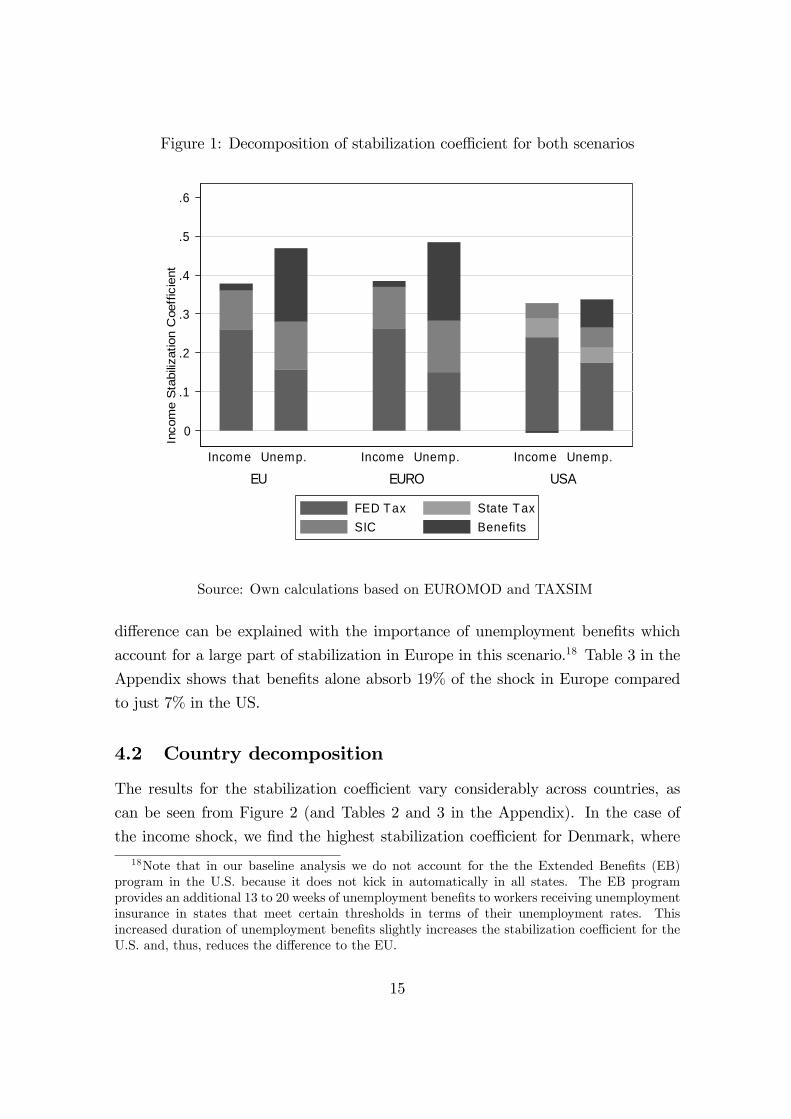
Figure 1: Decomposition of stabilization coe¢ cient for both scenarios

0

.1

.2

.3

.4

.5

.6

Inco

me 

Sta

biliz

atio

n C

oeff

icie

nt

EU EURO USAIncome Unemp. Income Unemp. Income Unemp.

FED Tax State TaxSIC Benefi ts

Source: Own calculations based on EUROMOD and TAXSIM

di¤erence can be explained with the importance of unemployment bene�ts which

account for a large part of stabilization in Europe in this scenario.18 Table 3 in the

Appendix shows that bene�ts alone absorb 19% of the shock in Europe compared

to just 7% in the US.

4.2 Country decomposition

The results for the stabilization coe¢ cient vary considerably across countries, as

can be seen from Figure 2 (and Tables 2 and 3 in the Appendix). In the case of

the income shock, we �nd the highest stabilization coe¢ cient for Denmark, where

18Note that in our baseline analysis we do not account for the the Extended Bene�ts (EB)program in the U.S. because it does not kick in automatically in all states. The EB programprovides an additional 13 to 20 weeks of unemployment bene�ts to workers receiving unemploymentinsurance in states that meet certain thresholds in terms of their unemployment rates. Thisincreased duration of unemployment bene�ts slightly increases the stabilization coe¢ cient for theU.S. and, thus, reduces the di¤erence to the EU.

15

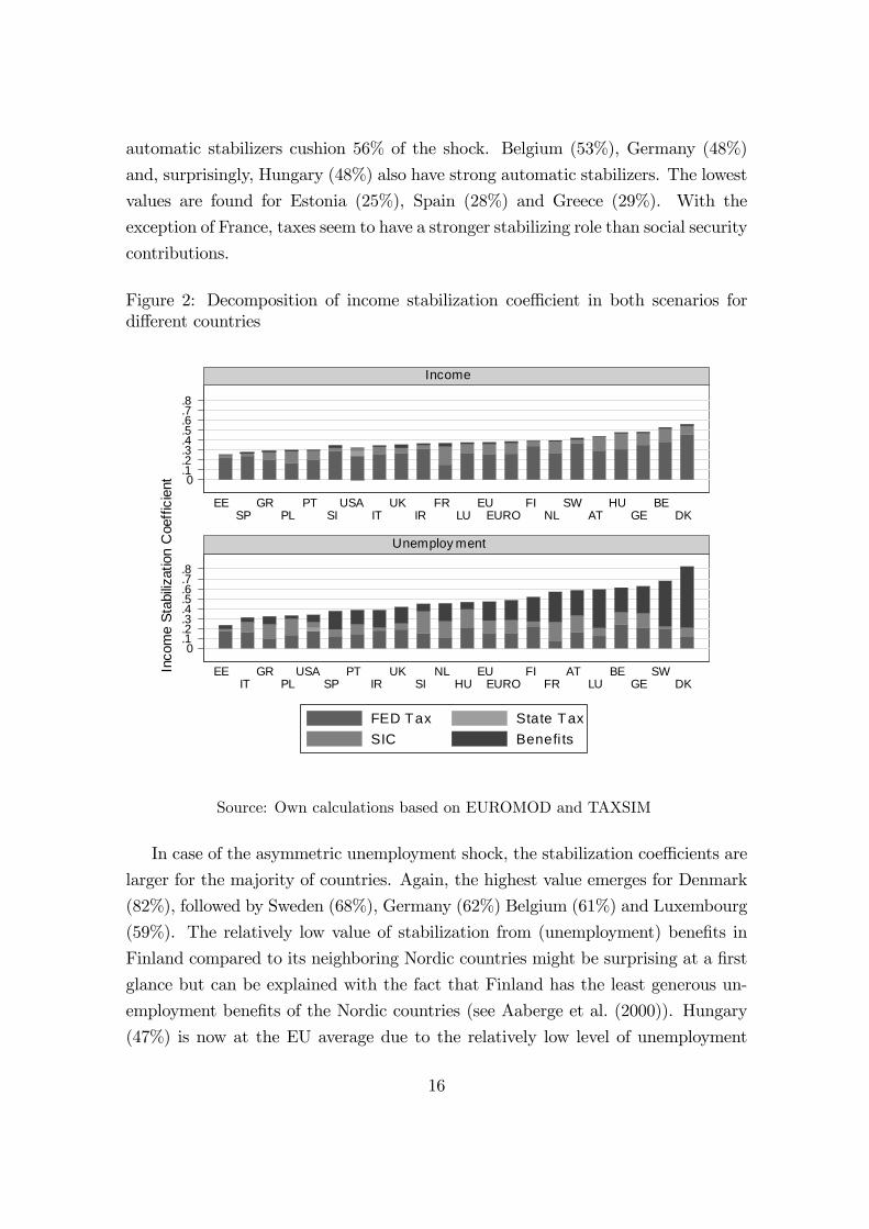
automatic stabilizers cushion 56% of the shock. Belgium (53%), Germany (48%)

and, surprisingly, Hungary (48%) also have strong automatic stabilizers. The lowest

values are found for Estonia (25%), Spain (28%) and Greece (29%). With the

exception of France, taxes seem to have a stronger stabilizing role than social security

contributions.

Figure 2: Decomposition of income stabilization coe¢ cient in both scenarios fordi¤erent countries

0.1.2.3.4.5.6.7.8

0.1.2.3.4.5.6.7.8

EESP

GRPL

PTSI

USAIT

UKIR

FRLU

EUEURO

FINL

SWAT

HUGE

BEDK

EEIT

GRPL

USASP

PTIR

UKSI

NLHU

EUEURO

FIFR

ATLU

BEGE

SWDK

Income

Unemploy ment

FED Tax State TaxSIC Benefi ts

Inco

me 

Stab

ilizat

ion 

Coe

ffici

ent

Source: Own calculations based on EUROMOD and TAXSIM

In case of the asymmetric unemployment shock, the stabilization coe¢ cients are

larger for the majority of countries. Again, the highest value emerges for Denmark

(82%), followed by Sweden (68%), Germany (62%) Belgium (61%) and Luxembourg

(59%). The relatively low value of stabilization from (unemployment) bene�ts in

Finland compared to its neighboring Nordic countries might be surprising at a �rst

glance but can be explained with the fact that Finland has the least generous un-

employment bene�ts of the Nordic countries (see Aaberge et al. (2000)). Hungary

(47%) is now at the EU average due to the relatively low level of unemployment

16

bene�ts. At the other end of the spectrum, there are some countries with values

below the US level of 34%. These include Estonia (23%), Italy (31%), and, to a

lesser extent, Poland (33%).

When looking only at the personal income tax, it is surprising that the values

for the US (federal and state level income tax combined) are higher than the EU

average. To some extent, this quali�es the widespread view that tax progressivity is

higher in Europe (e.g., Alesina and Glaeser (2004) or Piketty and Saez (2007)). Of

course, this can be partly explained by the considerable heterogeneity within Europe.

But still, only a few countries like Belgium, Germany and the Nordic countries have

higher contributions of stabilization coming from the personal income tax.

An interesting question is to what extent the results for the stabilization coef-

�cient are driven by the existing tax and transfer systems or by the demographic

characteristics in each country. To investigate this issue, we recalculate the income

stabilization coe¢ cients for each country under the given tax and transfer system,

but with the socio-demographic characteristics of each other country in our analysis.

This analysis yields a 20*20 matrix where the respective tax and transfer systems

are given in the columns and the demographics of each country in the rows. As

can be seen in Table 7, the income stabilization coe¢ cients computed under a �xed

tax and transfer system but with varying characteristics of the population do not

vary much. There is much more variation within a certain row (showing the income

stabilization coe¢ cients calculated with demographic characteristics of a certain

country but varying tax and transfer systems) than within a certain column (�xed

tax and transfer system of a certain country, but varying population characteris-

tics). Interestingly, the income stabilization coe¢ cient for the US is highest with

the socio-demographic characteristics of the US population whereas income stabi-

lization is (almost) lowest in countries such Italy, Portugal, Slovenia or the UK with

their given population characteristics.19 Thus, we conclude that the tax and trans-

fer rules and not the demographic characteristics are the main determinants of the

income stabilization coe¢ cient.

4.3 Demand stabilization

How does this cushioning of shocks translate into demand stabilization? The results

for stabilization of aggregate demand in the EU and the US are shown in Table

19We obtain similar results for the unemployment shock and the demand stabilization coe¢ cient.

17

1 and Figure 3.20 The demand stabilization coe¢ cients are lower than the income

stabilization coe¢ cients since demand stabilization can only be achieved for liquidity

constrained households. Moreover, there is considerable variation for the demand

stabilization coe¢ cient depending on the respective approach for the identi�cation

of liquidity constrained households. For the income shock (IS), results range from

4-22% for the EU and from 6-17% for the US. Taking the Zeldes criterion, i.e. net

wealth (based on asset income), as the determinant for liquidity constraints, demand

stabilization is 22% in the EU and 17% in the US. Demand stabilization coe¢ cients

which are based on direct survey evidence with respect to liquidity constraints on

average give the lower bound whereas those based on home ownership information

usually lie in between. For the unemployment shock (US), the EU-US gap widens

again. While in the US demand stabilization coe¢ cients mostly remain on their level

of the income shock, they are now substantially higher for the EU-group reaching

a peak of 30%. These results suggest that the transfers to the unemployed, in

particular the rather generous systems of unemployment insurance in Europe, play

a key role for demand stabilization and drive the di¤erence in automatic stabilizers

between Europe and the US.

For a more in-depth analysis taking into account country-speci�c results, it is use-

ful to consider �rst the shares of liquidity constrained households for each approach

as depicted in Table 4 in the Appendix. The Zeldes approach would suggest that

households are more likely to be liquidity constrained in Eastern than in Western

European countries because �nancial wealth is typically lower in the new member

states. Our estimates con�rm this as can be seen in Table 4.21 For this reason, auto-

matic stabilizers will be more important for demand stabilization in these countries,

at least if the Zeldes criterion is used for the identi�cation of liquidity constrained

households. A di¤erent picture emerges if home ownership is the determinant for

liquidity constraints. It is remarkable that the share of households who own their

homes is relatively high in Eastern and Southern European countries. This suggests

a lower share of liquidity constrained households and thus a lower contribution of

20Note that in Tables 1 and 4 as well as in Figure 3, the �rst approach for the identi�cation ofliquidity constraints refers to the �nancial wealth criterion (Zeldes), the second to the real estateproperty criterion (Runkle) and the third refers to survey evidence.

21As, according to the Zeldes criterion, liquidity constrained households are those householdswith low �nancial wealth and thus typically low income, one can expect that their share of income(IShare1) is lower than their share in the total population. In our data, this is true for all countries(see Table 4).

18

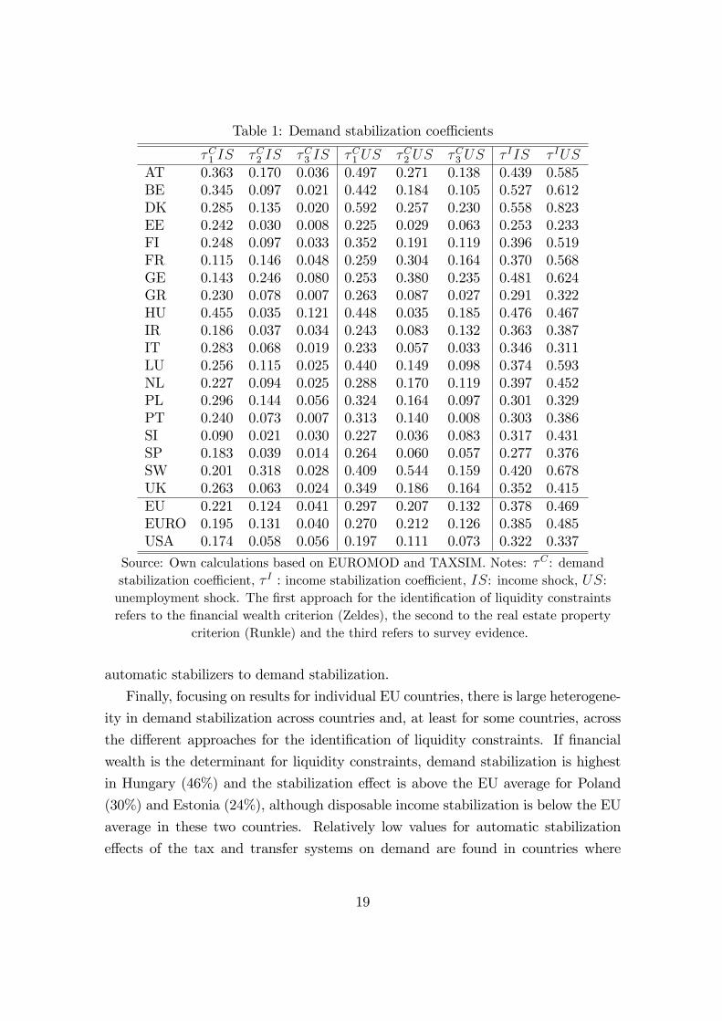
Table 1: Demand stabilization coe¢ cients

�C1 IS �C2 IS �C3 IS �C1 US �C2 US �C3 US � IIS � IUSAT 0.363 0.170 0.036 0.497 0.271 0.138 0.439 0.585BE 0.345 0.097 0.021 0.442 0.184 0.105 0.527 0.612DK 0.285 0.135 0.020 0.592 0.257 0.230 0.558 0.823EE 0.242 0.030 0.008 0.225 0.029 0.063 0.253 0.233FI 0.248 0.097 0.033 0.352 0.191 0.119 0.396 0.519FR 0.115 0.146 0.048 0.259 0.304 0.164 0.370 0.568GE 0.143 0.246 0.080 0.253 0.380 0.235 0.481 0.624GR 0.230 0.078 0.007 0.263 0.087 0.027 0.291 0.322HU 0.455 0.035 0.121 0.448 0.035 0.185 0.476 0.467IR 0.186 0.037 0.034 0.243 0.083 0.132 0.363 0.387IT 0.283 0.068 0.019 0.233 0.057 0.033 0.346 0.311LU 0.256 0.115 0.025 0.440 0.149 0.098 0.374 0.593NL 0.227 0.094 0.025 0.288 0.170 0.119 0.397 0.452PL 0.296 0.144 0.056 0.324 0.164 0.097 0.301 0.329PT 0.240 0.073 0.007 0.313 0.140 0.008 0.303 0.386SI 0.090 0.021 0.030 0.227 0.036 0.083 0.317 0.431SP 0.183 0.039 0.014 0.264 0.060 0.057 0.277 0.376SW 0.201 0.318 0.028 0.409 0.544 0.159 0.420 0.678UK 0.263 0.063 0.024 0.349 0.186 0.164 0.352 0.415EU 0.221 0.124 0.041 0.297 0.207 0.132 0.378 0.469EURO 0.195 0.131 0.040 0.270 0.212 0.126 0.385 0.485USA 0.174 0.058 0.056 0.197 0.111 0.073 0.322 0.337

Source: Own calculations based on EUROMOD and TAXSIM. Notes: �C : demandstabilization coe¢ cient, � I : income stabilization coe¢ cient, IS: income shock, US:unemployment shock. The �rst approach for the identi�cation of liquidity constraintsrefers to the �nancial wealth criterion (Zeldes), the second to the real estate property

criterion (Runkle) and the third refers to survey evidence.

automatic stabilizers to demand stabilization.

Finally, focusing on results for individual EU countries, there is large heterogene-

ity in demand stabilization across countries and, at least for some countries, across

the di¤erent approaches for the identi�cation of liquidity constraints. If �nancial

wealth is the determinant for liquidity constraints, demand stabilization is highest

in Hungary (46%) and the stabilization e¤ect is above the EU average for Poland

(30%) and Estonia (24%), although disposable income stabilization is below the EU

average in these two countries. Relatively low values for automatic stabilization

e¤ects of the tax and transfer systems on demand are found in countries where

19

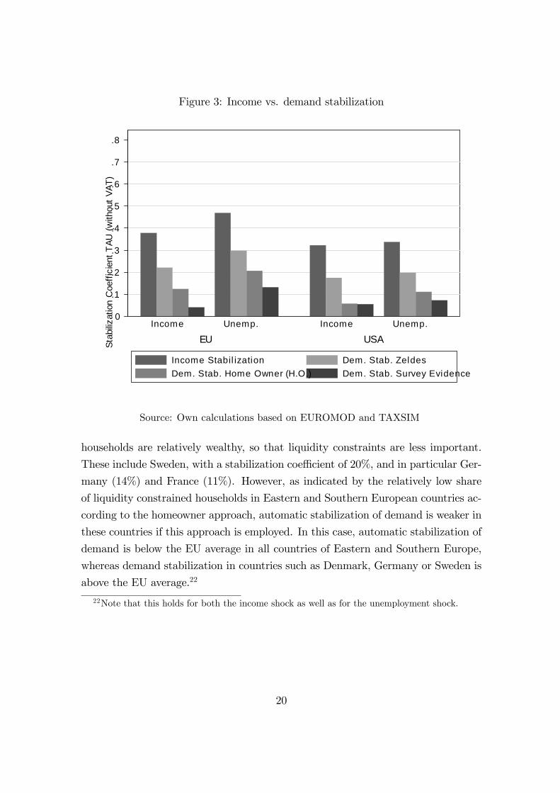
Figure 3: Income vs. demand stabilization

0

.1

.2

.3

.4

.5

.6

.7

.8

Stab

ilizat

ion 

Coe

ffici

ent T

AU (w

ithou

t VAT

)

EU USAIncome Unemp. Income Unemp.

Income Stabil ization Dem. Stab. ZeldesDem. Stab. Home Owner (H.O.) Dem. Stab. Survey Evidence

Source: Own calculations based on EUROMOD and TAXSIM

households are relatively wealthy, so that liquidity constraints are less important.

These include Sweden, with a stabilization coe¢ cient of 20%, and in particular Ger-

many (14%) and France (11%). However, as indicated by the relatively low share

of liquidity constrained households in Eastern and Southern European countries ac-

cording to the homeowner approach, automatic stabilization of demand is weaker in

these countries if this approach is employed. In this case, automatic stabilization of

demand is below the EU average in all countries of Eastern and Southern Europe,

whereas demand stabilization in countries such as Denmark, Germany or Sweden is

above the EU average.22

22Note that this holds for both the income shock as well as for the unemployment shock.

20

4.4 Extensions: Employer social insurance contributions and

consumption taxes

One limitation of our analysis is that we neglect various taxes which are certainly

relevant as automatic stabilizers and which di¤er in their relevance across countries.

In this section, we extend our analysis to employer social insurance contributions and

consumption taxes, which include value added, excise and sales taxes. We did not

include these taxes in our baseline simulations because they raise speci�c conceptual

issues.

4.4.1 Employer contributions

Consider �rst the case of employer social insurance contributions (or payroll taxes).

Including them requires us to make an assumption on their incidence. So far, we have

assumed that all taxes and transfers are borne by employees, so that a smoothing of

shocks through the tax and transfer system actually bene�ts the employees. We will

make the same assumption for employer social insurance contributions. This implies

that, in a hypothetical situation without taxes, social insurance contributions and

transfers, the income of household i would be gross income, which we de�ne as

follows:

Y Gi = Y Mi + SERi (9)

where Y Gi is gross income, Y Mi market income and SERi employer social insurance

contributions. We now consider a shock to gross income and ask which part of

this shock is absorbed by the tax and transfer system. The income stabilization

coe¢ cient is now given by

� I =Xf

� If =

Pi

��Ti +�Si +�S

ERi ��Bi

�Pi�Y

Gi

:

How does the inclusion of employer social insurance contributions a¤ect the

stabilization e¤ects? For the EU, the income stabilization coe¢ cient is now equal

to 48% for the income shock and 56% for the unemployment shock. For the US, we

�nd respective values of 36% for the income shock and 39% for the unemployment

shock. The results by country are given in Table 5 in the Appendix.23 In countries

23Note that, when comparing these results to those of our baseline simulation, it has to be taken

21

such as Italy or Sweden, employer social insurance contributions make up a large

proportion of total contributions leading to a substantial increase in stabilization

through SIC in these countries. However, the results cannot be compared directly

to those of the preceding section because the stabilization e¤ect is now measured in

per cent of a shock to Y Gi , not YMi .

4.4.2 Consumption taxes

How can consumption taxes be integrated into this framework? In order to make

the results comparable to our baseline simulations, we return to the case where we

exclude employer social insurance contributions from the analysis. The data we

use includes no information on consumption expenditures of households, so that

the consumption taxes actually paid cannot be calculated directly. Instead, we use

implicit tax rates (ITR) on consumption taken from European Commission (2009b)

for European countries and McIntyre et al. (2003) for the US. The ITR is a measure

for the e¤ective tax burden which includes several consumption taxes such as VAT or

sales taxes, energy and other excise taxes. This implicit tax rate relates consumption

taxes paid to overall consumption. Given this, we can write the budget constraint

of household i as

Y Mi = Ci(1 + tC) + Ai + Ti + Si �Bi

where tC is the implicit consumption tax rate, TC = tCC the consumption tax

payments, and Ai represents savings.

What is the role of the consumption tax for automatic stabilization? This de-

pends on the reaction of consumption to the income shock. Our analysis assumes

that only liquidity constrained households will adjust their consumption to an in-

come shock. An automatic stabilization e¤ect of consumption taxes can only occur

for these households, where changes in disposable income are equal to changes in

consumption and, hence, consumption tax payments. Given this, we focus on de-

mand, rather than income stabilization through the consumption tax. The demand

stabilization coe¢ cient can now be written as:

�Ct =

Ph

��TCh +�Th +�Sh ��Bh

�Pi�Y

Mi

(10)

into account that we now consider a shock on Y Gi , not on YMi . This explains, for instance, why

the measured stabilization coe¢ cient of income taxes is now lower.

22

where h is the index for the liquidity constrained households.

The results are given in Table 6 in the Appendix: Demand stabilization through

the consumption tax (according to the �nancial wealth criterion) is higher in the EU

than in the US. Within the EU, we �nd highest stabilization coe¢ cients in Eastern

European countries which can again be explained by the high proportion of liquidity

constrained households and a relatively higher share of direct taxes.

5 Discussion of the results

In this section, we discuss a number of possible objections to and questions raised

by our analysis. These include the relation of our results to widely used macro

indicators of automatic stabilizers, the role of other taxes, the correlation between

automatic stabilizers and other macro variables like e.g. openness and, �nally, the

correlations between discretionary �scal stimulus programs and automatic stabilizers

as well as openness.

5.1 Stabilization coe¢ cients and simple macro indicators

One could argue that macro measures like e.g. the tax revenue to GDP ratio reveal

su¢ cient information on the magnitude of automatic stabilizers in the di¤erent

countries. For instance, the IMF (2009) has recently used aggregate tax to GDP

ratios as proxies for the size of automatic stabilizers in G-20 countries. The upper

panel of Figure 4 depicts the relation between the ratio of average revenue 2006-2010

to GDP and the income stabilization coe¢ cient for the proportional income shock.24

With a correlation of 0.58, one can conclude that government size is indeed a good

predictor for the amount of automatic stabilization. The picture changes, however,

if stabilization of aggregate household demand is considered, i.e. if we account for

liquidity constraints.25 As shown in Figure 4 (lower panel), with a coe¢ cient of 0.26

government size and stabilization of aggregate household demand are only weakly

correlated.26

24All �gures and correlations in this section are population-weighted in order to control fordi¤erent country sizes. However, results are similar to those without population-weighting. Wealso obtained similar results when using the government spending to GDP ratio instead of revenueas a measure of the size of the government.

25In this section, we always refer to the demand stabilization coe¢ cient based on the Zeldescriterion.

26The respective correlations for the unemployment shock are 0.69 and 0.65.

23

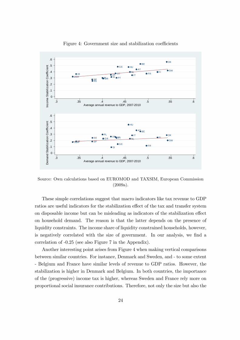
Figure 4: Government size and stabilization coe¢ cients

AT

BEDK

EE

FIFR

GE

GR

HU

IR ITLU NL

PL PTSISP

SW

UKUSA

0

.1

.2

.3

.4

.5

.6

Inco

me 

Sta

biliz

atio

n C

oeffi

cien

t

.3 .35 .4 .45 .5 .55 .6Average annual revenue to GDP, 2007­2010

AT BEDK

EE FI

FRGE

GR

HU

IR

ITLU

NL

PLPT

SI

SP SWUK

USA

0

.1

.2

.3

.4

.5

.6

Dem

and 

Stab

iliza

tion 

Coe

ffici

ent

.3 .35 .4 .45 .5 .55 .6Average annual revenue to GDP, 2007­2010

Source: Own calculations based on EUROMOD and TAXSIM, European Commission(2009a).

These simple correlations suggest that macro indicators like tax revenue to GDP

ratios are useful indicators for the stabilization e¤ect of the tax and transfer system

on disposable income but can be misleading as indicators of the stabilization e¤ect

on household demand. The reason is that the latter depends on the presence of

liquidity constraints. The income share of liquidity constrained households, however,

is negatively correlated with the size of government. In our analysis, we �nd a

correlation of -0.25 (see also Figure 7 in the Appendix).

Another interesting point arises from Figure 4 when making vertical comparisons

between similar countries. For instance, Denmark and Sweden, and - to some extent

- Belgium and France have similar levels of revenue to GDP ratios. However, the

stabilization is higher in Denmark and Belgium. In both countries, the importance

of the (progressive) income tax is higher, whereas Sweden and France rely more on

proportional social insurance contributions. Therefore, not only the size but also the

24

structure of the tax bene�t system are important for its possibilities of automatic

stabilization.

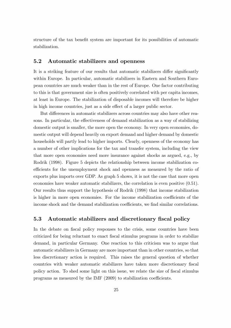
5.2 Automatic stabilizers and openness

It is a striking feature of our results that automatic stabilizers di¤er signi�cantly

within Europe. In particular, automatic stabilizers in Eastern and Southern Euro-

pean countries are much weaker than in the rest of Europe. One factor contributing

to this is that government size is often positively correlated with per capita incomes,

at least in Europe. The stabilization of disposable incomes will therefore be higher

in high income countries, just as a side e¤ect of a larger public sector.

But di¤erences in automatic stabilizers across countries may also have other rea-

sons. In particular, the e¤ectiveness of demand stabilization as a way of stabilizing

domestic output is smaller, the more open the economy. In very open economies, do-

mestic output will depend heavily on export demand and higher demand by domestic

households will partly lead to higher imports. Clearly, openness of the economy has

a number of other implications for the tax and transfer system, including the view

that more open economies need more insurance against shocks as argued, e.g., by

Rodrik (1998). Figure 5 depicts the relationship between income stabilization co-

e¢ cients for the unemployment shock and openness as measured by the ratio of

exports plus imports over GDP. As graph 5 shows, it is not the case that more open

economies have weaker automatic stabilizers, the correlation is even positive (0.51).

Our results thus support the hypothesis of Rodrik (1998) that income stabilization

is higher in more open economies. For the income stabilization coe¢ cients of the

income shock and the demand stabilization coe¢ cients, we �nd similar correlations.

5.3 Automatic stabilizers and discretionary �scal policy

In the debate on �scal policy responses to the crisis, some countries have been

criticized for being reluctant to enact �scal stimulus programs in order to stabilize

demand, in particular Germany. One reaction to this criticism was to argue that

automatic stabilizers in Germany are more important than in other countries, so that

less discretionary action is required. This raises the general question of whether

countries with weaker automatic stabilizers have taken more discretionary �scal

policy action. To shed some light on this issue, we relate the size of �scal stimulus

programs as measured by the IMF (2009) to stabilization coe¢ cients.

25

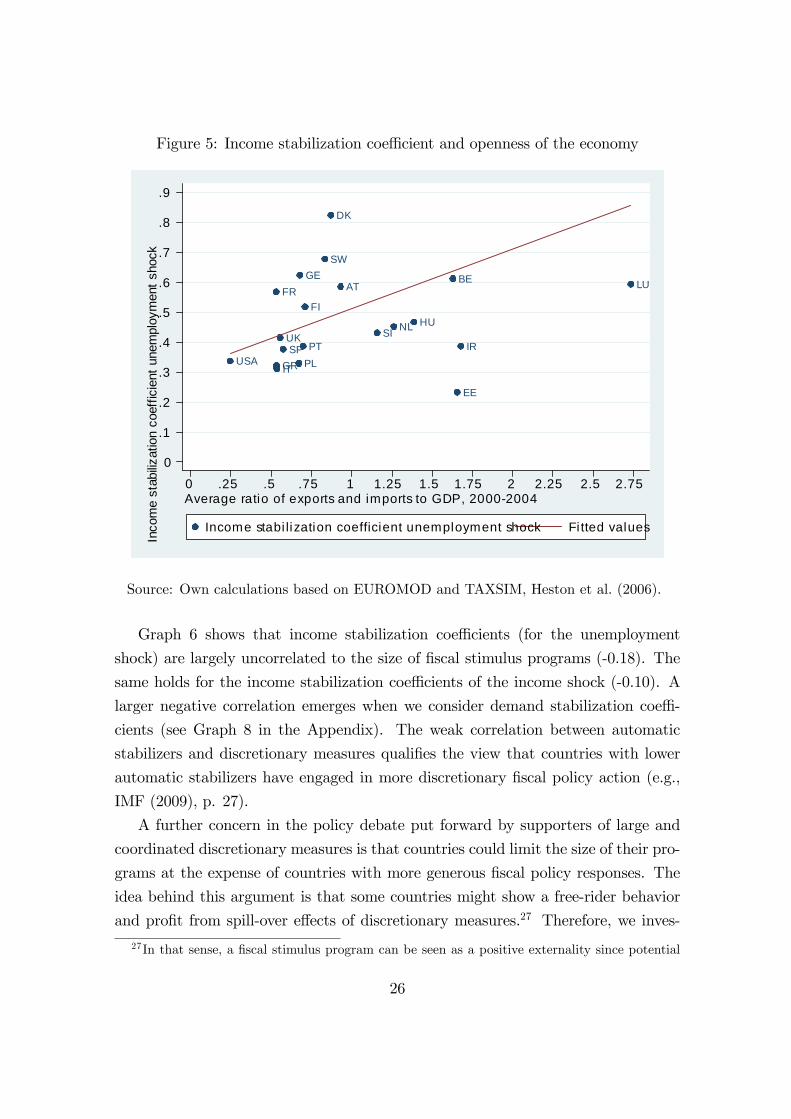
Figure 5: Income stabilization coe¢ cient and openness of the economy

ATBE

DK

EE

FIFR

GE

GR

HU

IR

IT

LU

NL

PLPT

SISP

SW

UK

USA

0

.1

.2

.3

.4

.5

.6

.7

.8

.9

Inco

me 

stab

ilizat

ion 

coef

ficie

nt u

nem

ploy

men

t sho

ck

0 .25 .5 .75 1 1.25 1.5 1.75 2 2.25 2.5 2.75Average ratio of exports and imports to GDP, 2000­2004

Income stabi lization coefficient unemployment shock Fitted values

Source: Own calculations based on EUROMOD and TAXSIM, Heston et al. (2006).

Graph 6 shows that income stabilization coe¢ cients (for the unemployment

shock) are largely uncorrelated to the size of �scal stimulus programs (-0.18). The

same holds for the income stabilization coe¢ cients of the income shock (-0.10). A

larger negative correlation emerges when we consider demand stabilization coe¢ -

cients (see Graph 8 in the Appendix). The weak correlation between automatic

stabilizers and discretionary measures quali�es the view that countries with lower

automatic stabilizers have engaged in more discretionary �scal policy action (e.g.,

IMF (2009), p. 27).

A further concern in the policy debate put forward by supporters of large and

coordinated discretionary measures is that countries could limit the size of their pro-

grams at the expense of countries with more generous �scal policy responses. The

idea behind this argument is that some countries might show a free-rider behavior

and pro�t from spill-over e¤ects of discretionary measures.27 Therefore, we inves-

27In that sense, a �scal stimulus program can be seen as a positive externality since potential

26

Figure 6: Discretionary measures and income stabilization coe¢ cient

AT

BEDK

EE

FI

FR

GE

GR

HU

IRIT

LU

NL

PL

PT

SI

SP

SW

UK

USA

0

.005

.01

.015

.02

.025

Aver

age 

annu

al d

iscr

etio

nary

 mea

sure

s 20

09­2

010

.2 .3 .4 .5 .6 .7 .8 .9Income stabi lization coefficient unemployment shock

Average annual discretionary measures 2009­2010 Fitted values

Source: Own calculations based on EUROMOD and TAXSIM, European Commission(2009c), IMF (2009) and International Labour O¢ ce and International Institute for

Labour Studies (2009).

tigate the hypothesis if more open countries which are supposed to bene�t more

from spill-over e¤ects indeed passed smaller stimulus programs. We �nd a negative

correlation of -0.40 between the average annual discretionary measures in 2009 and

2010 and the coe¢ cient for openness which supports the hypothesis.28

positive e¤ects are not limited to the country of origin.28Cf. Graph 9 in the Appendix. A multivariate regression of discretionary measures on the

income stabilization coe¢ cients, a measure of openness of the respective economies and theirgovernments�budget balance in 2007 leads to signi�cant coe¢ cients of openness and the budgetbalance; whereas the relationship between discretionary �scal policy and the amount of automaticstabilization remains insigni�cant. This result indicates that in addition to the argument aboveabout openness, some governments have been constrained by weak budget positions in their decisionmaking about discretionary �scal policy. However, due to the very small sample size, this inferenceshould be interpreted with caution.

27

6 Conclusions

In this paper we have used microsimulation models for the tax and transfer sys-

tems of 19 European countries (EUROMOD) and the US (TAXSIM) to investigate

the extent to which automatic stabilizers cushion household disposable income and

household demand in the event of macroeconomic shocks. Our baseline simulations

focus on the personal income tax, employee social insurance contributions and ben-

e�ts. We �nd that the amount of automatic stabilization depends strongly on the

type of income shock. In the case of a proportional income shock, approximately

38% of the shock would be absorbed by automatic stabilizers in the EU. For the

US, we �nd a value of 32%. Within the EU, there is considerable heterogeneity,

and results range from a value of 25% for Estonia to 56% for Denmark. In general

automatic stabilizers in Eastern and Southern European countries are considerably

lower than in Continental and Northern European countries.

In the case of an unemployment shock, which a¤ects households asymmetrically,

the di¤erence between the EU and the US is larger. EU automatic stabilizers absorb

47% of the shock whereas the stabilization e¤ect in the US is only 34%. Again,

there is considerable heterogeneity within the EU. This result implies that European

welfare states provide higher insurance against idiosyncratic shocks than the US

does. In addition, our analysis shows that the results for the proportional income

shock do not di¤er much to a proportional income increase (results available from

the authors upon request). Hence, the di¤erence between the income shock and

the unemployment shock can also be interpreted as the di¤erent size of automatic

stabilization in good and bad times.

These results suggest that social transfers, in particular the rather generous sys-

tems of unemployment insurance in Europe, play a key role for the stabilization of

disposable incomes and household demand and explain a large part of the di¤erence

in automatic stabilizers between Europe and the US. This is con�rmed by the de-

composition of stabilization e¤ects in our analysis. In the case of the unemployment

shocks, bene�ts alone absorb 19% of the shock in Europe compared to just 7% in the

US, whereas the stabilizing e¤ect of income taxes (taking into account State taxes

in the US as well) is similar. To some extent, this quali�es the view that automatic

stabilizers are larger in Europe than in the US. This is only true for countries like

Belgium, Denmark, Finland, Germany or Sweden.

How does this cushioning of shocks translate into demand stabilization? Since

28

demand stabilization can only be achieved for liquidity constrained households, the

picture changes signi�cantly. For the proportional income shock, the cushioning

e¤ect of automatic stabilizers ranges from 4-22% in the EU. For the US, we �nd

values between 6-17%, which is again rather similar. The values for the Euro area

are close to those for the EU. For the unemployment shock, however, we �nd a large

di¤erence. In the EU, the stabilization e¤ect ranges from 13-30% whereas the values

for the US (7-20%) are close to those for the income shock.

A second key result of our analysis is that demand stabilization di¤ers consider-

ably from disposable income stabilization. This has important policy implications,

also for discretionary �scal policy. Focusing on income stabilization may lead poli-

cymakers to overestimate the e¤ect of automatic stabilizers.

A third important result of our analysis is that automatic stabilizers are very

heterogenous within Europe. Interestingly, Eastern and Southern European coun-

tries are characterized by rather low automatic stabilizers. This is surprising, at

least from an insurance point of view because lower average income (and wealth)

implies that households are more vulnerable to income shocks. One explanation

for this �nding could be that countries with lower per capita incomes tend to have

smaller public sectors. From this perspective, weaker automatic stabilizers in East-

ern and Southern European countries are a potentially unintended side e¤ect of the

lower demand for government activity including redistribution. Another potential

explanation, the idea that more open economies have weaker automatic stabilizers

because domestic demand spills over to other countries, seems to be inconsistent with

the data, at least as far as the simple correlation between stabilization coe¢ cients

and trade to GDP ratios is concerned.

Finally, we have discussed the claim that countries with smaller automatic sta-

bilizers have engaged in more discretionary �scal policy action. According to our

results, there is no correlation between �scal stimulus programs of individual coun-

tries and stabilization coe¢ cients. However, we �nd that more open countries and

countries with higher budget de�cits have passed smaller stimulus programs. All

in all, our results suggest that policymakers did not take into account the forces

of automatic stabilizers when designing active �scal policy measures to tackle the

current economic crisis.

These results have to be interpreted in the light of various limitations of our

analysis. Firstly, the role of tax and transfer systems for stabilizing household

demand, not just disposable income, is based on strong assumptions on the link

29

between disposable income and household expenditures. Although we have used

what we believe to be the best available methods for estimating liquidity constraints,

considerable uncertainty remains as to whether these methods lead to an appropriate

description of household behavior. Secondly, our analysis abstracts from automatic

stabilization through other taxes, in particular corporate income taxes. Thirdly, our

analysis is purely positive. We abstract from normative welfare considerations about

the optimal size of automatic stabilization. Taxes are distortionary and hence imply

a trade-o¤ between insurance against shocks through redistribution and e¢ ciency

considerations. Finally, we have abstracted from the role of labor supply or other

behavioral adjustments for the impact of automatic stabilizers. We intend to pursue

these issues in future research.

30

A Appendix:

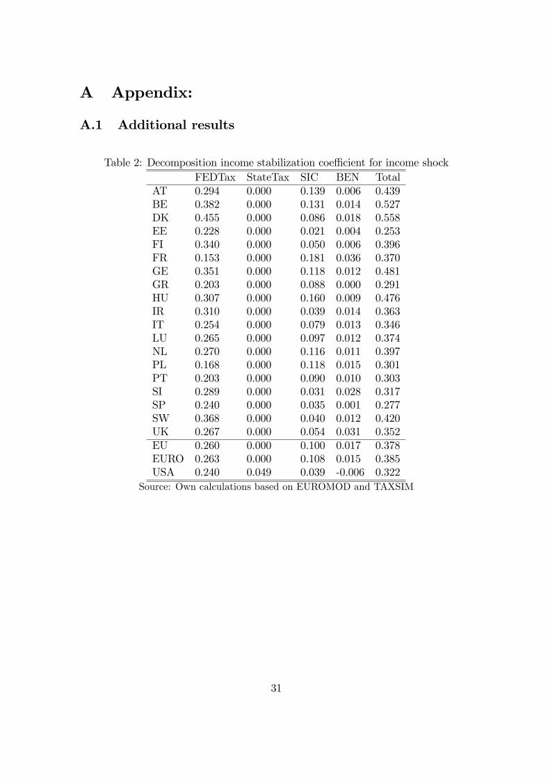
A.1 Additional results

Table 2: Decomposition income stabilization coe¢ cient for income shockFEDTax StateTax SIC BEN Total

AT 0.294 0.000 0.139 0.006 0.439BE 0.382 0.000 0.131 0.014 0.527DK 0.455 0.000 0.086 0.018 0.558EE 0.228 0.000 0.021 0.004 0.253FI 0.340 0.000 0.050 0.006 0.396FR 0.153 0.000 0.181 0.036 0.370GE 0.351 0.000 0.118 0.012 0.481GR 0.203 0.000 0.088 0.000 0.291HU 0.307 0.000 0.160 0.009 0.476IR 0.310 0.000 0.039 0.014 0.363IT 0.254 0.000 0.079 0.013 0.346LU 0.265 0.000 0.097 0.012 0.374NL 0.270 0.000 0.116 0.011 0.397PL 0.168 0.000 0.118 0.015 0.301PT 0.203 0.000 0.090 0.010 0.303SI 0.289 0.000 0.031 0.028 0.317SP 0.240 0.000 0.035 0.001 0.277SW 0.368 0.000 0.040 0.012 0.420UK 0.267 0.000 0.054 0.031 0.352EU 0.260 0.000 0.100 0.017 0.378EURO 0.263 0.000 0.108 0.015 0.385USA 0.240 0.049 0.039 -0.006 0.322

Source: Own calculations based on EUROMOD and TAXSIM

31

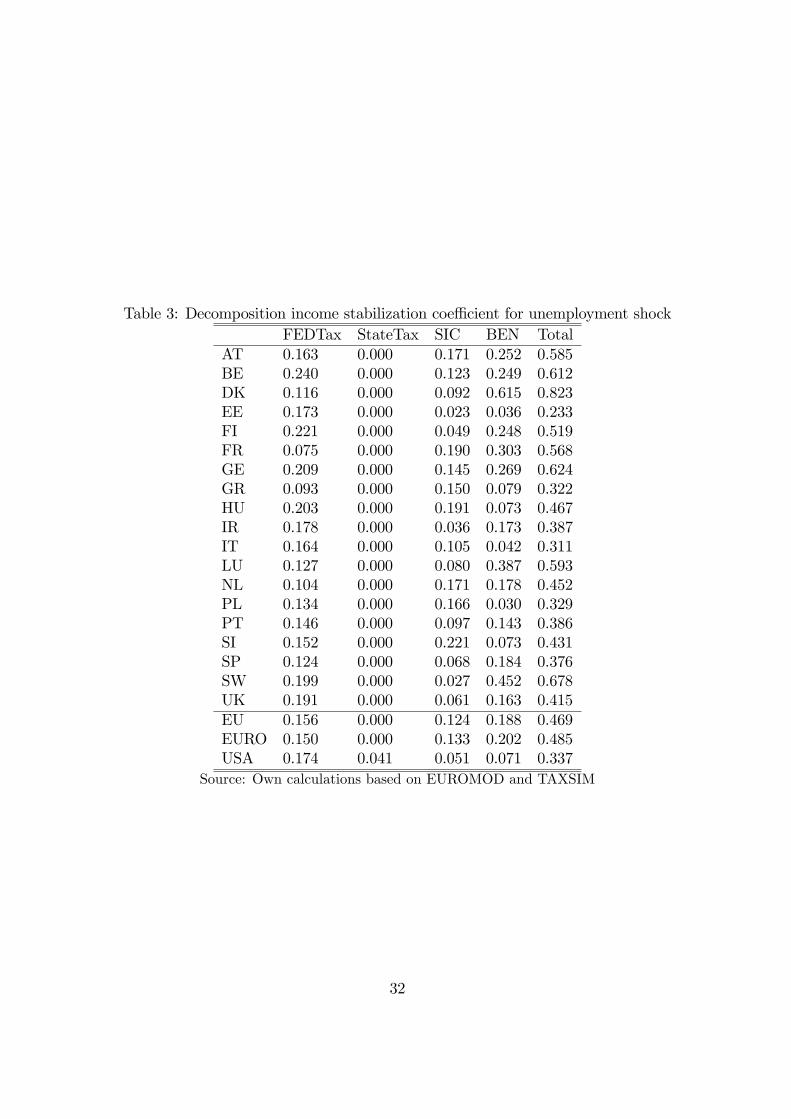
Table 3: Decomposition income stabilization coe¢ cient for unemployment shockFEDTax StateTax SIC BEN Total

AT 0.163 0.000 0.171 0.252 0.585BE 0.240 0.000 0.123 0.249 0.612DK 0.116 0.000 0.092 0.615 0.823EE 0.173 0.000 0.023 0.036 0.233FI 0.221 0.000 0.049 0.248 0.519FR 0.075 0.000 0.190 0.303 0.568GE 0.209 0.000 0.145 0.269 0.624GR 0.093 0.000 0.150 0.079 0.322HU 0.203 0.000 0.191 0.073 0.467IR 0.178 0.000 0.036 0.173 0.387IT 0.164 0.000 0.105 0.042 0.311LU 0.127 0.000 0.080 0.387 0.593NL 0.104 0.000 0.171 0.178 0.452PL 0.134 0.000 0.166 0.030 0.329PT 0.146 0.000 0.097 0.143 0.386SI 0.152 0.000 0.221 0.073 0.431SP 0.124 0.000 0.068 0.184 0.376SW 0.199 0.000 0.027 0.452 0.678UK 0.191 0.000 0.061 0.163 0.415EU 0.156 0.000 0.124 0.188 0.469EURO 0.150 0.000 0.133 0.202 0.485USA 0.174 0.041 0.051 0.071 0.337

Source: Own calculations based on EUROMOD and TAXSIM

32

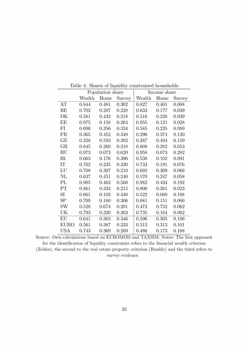
Table 4: Shares of liquidity constrained householdsPopulation share Income share

Wealth Home Survey Wealth Home SurveyAT 0.844 0.481 0.302 0.827 0.401 0.088BE 0.702 0.297 0.228 0.633 0.177 0.039DK 0.581 0.432 0.218 0.516 0.238 0.039EE 0.975 0.158 0.264 0.955 0.121 0.028FI 0.696 0.356 0.334 0.585 0.235 0.089FR 0.365 0.452 0.340 0.296 0.374 0.120GE 0.328 0.593 0.392 0.287 0.494 0.159GR 0.845 0.260 0.318 0.808 0.282 0.053HU 0.973 0.073 0.620 0.958 0.073 0.282IR 0.663 0.176 0.396 0.538 0.102 0.091IT 0.762 0.235 0.330 0.733 0.191 0.076LU 0.708 0.307 0.210 0.692 0.309 0.066NL 0.637 0.451 0.240 0.570 0.247 0.058PL 0.985 0.463 0.560 0.982 0.434 0.192PT 0.861 0.334 0.215 0.800 0.261 0.023SI 0.661 0.103 0.440 0.522 0.080 0.108SP 0.709 0.180 0.306 0.681 0.151 0.066SW 0.528 0.674 0.201 0.472 0.752 0.062UK 0.793 0.320 0.263 0.735 0.164 0.062EU 0.641 0.383 0.346 0.596 0.305 0.106EURO 0.561 0.387 0.333 0.513 0.313 0.101USA 0.743 0.369 0.269 0.486 0.173 0.168

Source: Own calculations based on EUROMOD and TAXSIM. Notes: The �rst approachfor the identi�cation of liquidity constraints refers to the �nancial wealth criterion

(Zeldes), the second to the real estate property criterion (Runkle) and the third refers tosurvey evidence.

33

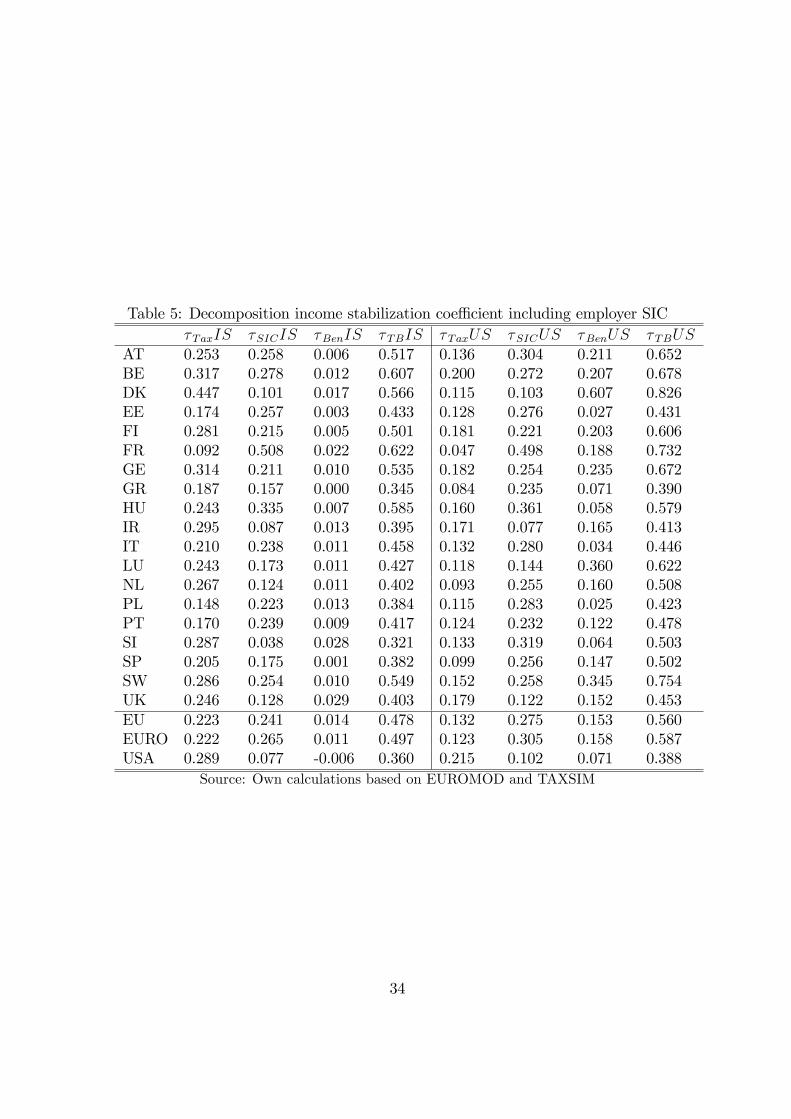
Table 5: Decomposition income stabilization coe¢ cient including employer SIC�TaxIS �SICIS �BenIS �TBIS �TaxUS �SICUS �BenUS �TBUS

AT 0.253 0.258 0.006 0.517 0.136 0.304 0.211 0.652BE 0.317 0.278 0.012 0.607 0.200 0.272 0.207 0.678DK 0.447 0.101 0.017 0.566 0.115 0.103 0.607 0.826EE 0.174 0.257 0.003 0.433 0.128 0.276 0.027 0.431FI 0.281 0.215 0.005 0.501 0.181 0.221 0.203 0.606FR 0.092 0.508 0.022 0.622 0.047 0.498 0.188 0.732GE 0.314 0.211 0.010 0.535 0.182 0.254 0.235 0.672GR 0.187 0.157 0.000 0.345 0.084 0.235 0.071 0.390HU 0.243 0.335 0.007 0.585 0.160 0.361 0.058 0.579IR 0.295 0.087 0.013 0.395 0.171 0.077 0.165 0.413IT 0.210 0.238 0.011 0.458 0.132 0.280 0.034 0.446LU 0.243 0.173 0.011 0.427 0.118 0.144 0.360 0.622NL 0.267 0.124 0.011 0.402 0.093 0.255 0.160 0.508PL 0.148 0.223 0.013 0.384 0.115 0.283 0.025 0.423PT 0.170 0.239 0.009 0.417 0.124 0.232 0.122 0.478SI 0.287 0.038 0.028 0.321 0.133 0.319 0.064 0.503SP 0.205 0.175 0.001 0.382 0.099 0.256 0.147 0.502SW 0.286 0.254 0.010 0.549 0.152 0.258 0.345 0.754UK 0.246 0.128 0.029 0.403 0.179 0.122 0.152 0.453EU 0.223 0.241 0.014 0.478 0.132 0.275 0.153 0.560EURO 0.222 0.265 0.011 0.497 0.123 0.305 0.158 0.587USA 0.289 0.077 -0.006 0.360 0.215 0.102 0.071 0.388

Source: Own calculations based on EUROMOD and TAXSIM

34

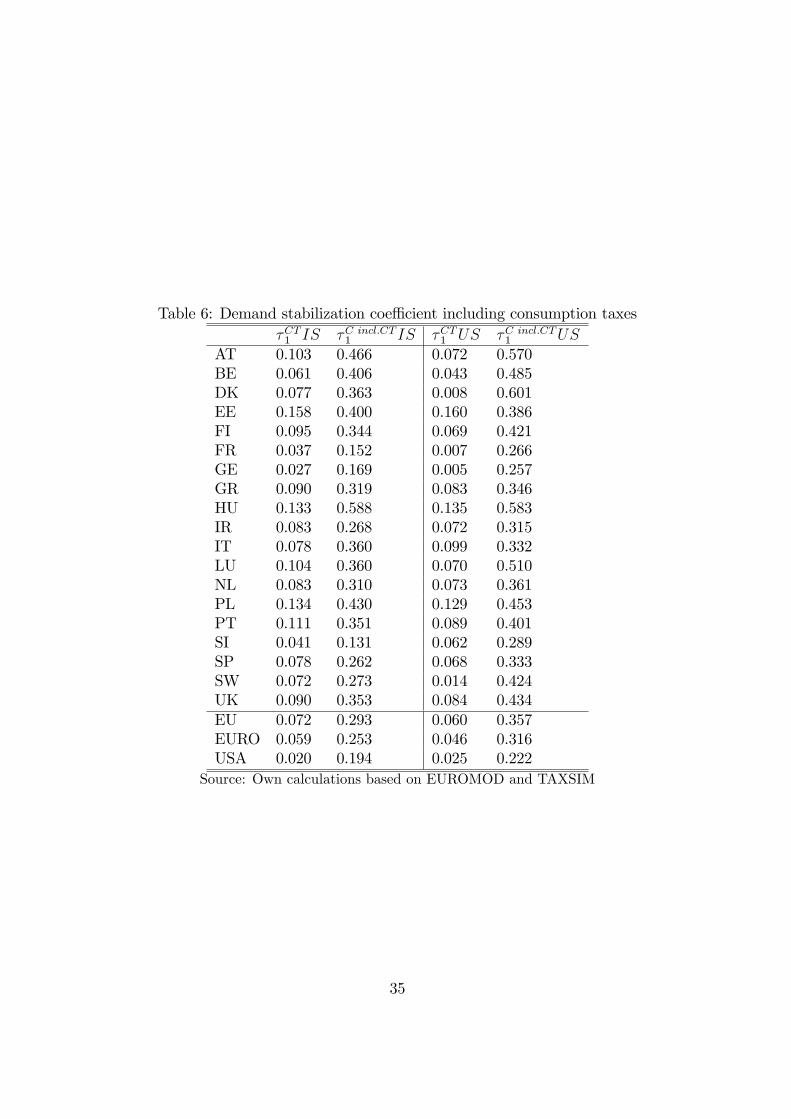
Table 6: Demand stabilization coe¢ cient including consumption taxes�CT1 IS �C incl:CT

1 IS �CT1 US �C incl:CT1 US

AT 0.103 0.466 0.072 0.570BE 0.061 0.406 0.043 0.485DK 0.077 0.363 0.008 0.601EE 0.158 0.400 0.160 0.386FI 0.095 0.344 0.069 0.421FR 0.037 0.152 0.007 0.266GE 0.027 0.169 0.005 0.257GR 0.090 0.319 0.083 0.346HU 0.133 0.588 0.135 0.583IR 0.083 0.268 0.072 0.315IT 0.078 0.360 0.099 0.332LU 0.104 0.360 0.070 0.510NL 0.083 0.310 0.073 0.361PL 0.134 0.430 0.129 0.453PT 0.111 0.351 0.089 0.401SI 0.041 0.131 0.062 0.289SP 0.078 0.262 0.068 0.333SW 0.072 0.273 0.014 0.424UK 0.090 0.353 0.084 0.434EU 0.072 0.293 0.060 0.357EURO 0.059 0.253 0.046 0.316USA 0.020 0.194 0.025 0.222

Source: Own calculations based on EUROMOD and TAXSIM

35

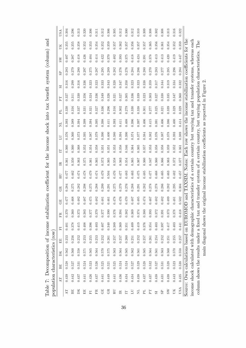
Table7:Decompositionofincomestabilizationcoe¢cientfortheincomeshockintotaxbene�tsystem

(column)and

populationcharacteristics(row)

AT

BE

DK

EE

FI

FR

GE

GR

HU

IRIT

LU

NL

PL

PT

SI

SP

SW

UK

USA

AT

0.439

0.528

0.562

0.253

0.401

0.370

0.477

0.284

0.477

0.361

0.360

0.376

0.393

0.330

0.327

0.316

0.283

0.407

0.355

0.304

BE

0.442

0.527

0.560

0.256

0.378

0.360

0.468

0.275

0.462

0.350

0.360

0.360

0.389

0.316

0.311

0.299

0.279

0.387

0.355

0.296

DK

0.437

0.531

0.558

0.252

0.415

0.373

0.482

0.282

0.474

0.363

0.368

0.373

0.394

0.337

0.330

0.316

0.280

0.418

0.358

0.313

EE

0.441

0.524

0.571

0.253

0.408

0.383

0.487

0.298

0.478

0.375

0.352

0.395

0.399

0.331

0.356

0.336

0.297

0.426

0.352

0.320

FI

0.426

0.523

0.565

0.255

0.396

0.377

0.475

0.275

0.479

0.361

0.354

0.387

0.394

0.321

0.324

0.323

0.275

0.404

0.353

0.306

FR

0.437

0.526

0.564

0.253

0.403

0.370

0.482

0.288

0.474

0.365

0.358

0.379

0.395

0.327

0.336

0.323

0.287

0.414

0.354

0.311

GE

0.441

0.525

0.570

0.252

0.407

0.377

0.481

0.299

0.479

0.373

0.351

0.390

0.398

0.336

0.349

0.333

0.295

0.422

0.352

0.312

GR

0.449

0.521

0.575

0.261

0.340

0.390

0.461

0.291

0.504

0.365

0.351

0.400

0.411

0.296

0.326

0.343

0.289

0.370

0.359

0.306

HU

0.441

0.525

0.563

0.257

0.389

0.376

0.478

0.275

0.476

0.358

0.353

0.380

0.393

0.316

0.321

0.320

0.282

0.402

0.357

0.305

IR0.436

0.524

0.564

0.257

0.369

0.394

0.476

0.279

0.477

0.363

0.358

0.394

0.411

0.302

0.327

0.347

0.276

0.393

0.362

0.312

IT0.434

0.524

0.565

0.260

0.351

0.382

0.470

0.276

0.483

0.354

0.346

0.390

0.408

0.279

0.305

0.350

0.276

0.375

0.357

0.300

LU

0.434

0.527

0.562

0.251

0.409

0.369

0.487

0.288

0.463

0.365

0.364

0.374

0.396

0.330

0.336

0.323

0.284

0.418

0.356

0.312

NL

0.438

0.529

0.561

0.252

0.419

0.374

0.485

0.291

0.475

0.367

0.365

0.377

0.397

0.338

0.339

0.323

0.286

0.424

0.357

0.310

PL

0.437

0.528

0.565

0.257

0.376

0.380

0.474

0.282

0.485

0.360

0.357

0.384

0.406

0.301

0.323

0.338

0.280

0.391

0.357

0.309

PT

0.437

0.532

0.564

0.261

0.354

0.393

0.467

0.278

0.477

0.347

0.353

0.382

0.415

0.277

0.303

0.359

0.270

0.378

0.365

0.308

SI

0.438

0.527

0.561

0.254

0.403

0.372

0.482

0.278

0.468

0.360

0.358

0.376

0.391

0.325

0.327

0.317

0.283

0.413

0.356

0.302

SP

0.431

0.531

0.563

0.252

0.397

0.391

0.482

0.286

0.465

0.366

0.358

0.387

0.406

0.321

0.338

0.344

0.277

0.413

0.361

0.308

SW

0.438

0.528

0.560

0.251

0.417

0.373

0.489

0.282

0.463

0.363

0.359

0.378

0.386

0.339

0.335

0.319

0.285

0.420

0.354

0.313

UK

0.443

0.523

0.570

0.255

0.403

0.378

0.481

0.295

0.482

0.372

0.352

0.393

0.400

0.329

0.347

0.334

0.296

0.419

0.352

0.316

USA

0.435

0.538

0.558

0.257

0.441

0.418

0.502

0.304

0.457

0.377

0.361

0.389

0.414

0.329

0.360

0.332

0.284

0.447

0.359

0.322

Source:OwncalculationsbasedonEUROMODandTAXSIM.Notes:Eachrowshowstheincomestabilizationcoe¢cientsforthe

incomeshockcalculatedwithdemographiccharacteristicsofacertaincountrybutvaryingtaxandtransfersystems,whereaseach

columnshowstheresultsundera�xedtaxandtransfersystem

ofacertaincountry,butvaryingpopulationcharacteristics.The

maindiagonalshowstheoriginalincomestabilizationcoe¢cientsasreportedinFigure2.

36

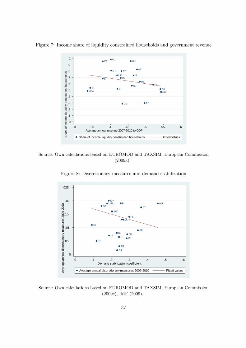
Figure 7: Income share of liquidity constrained households and government revenue

AT

BE

DK

EE

FI

FRGE

GR

HU

IR

ITLU

NL

PL

PT

SI

SP

SW

UK

USA

0

.1

.2

.3

.4

.5

.6

.7

.8

.9

1

Sha

re o

f inc

ome 

liqui

dity

 con

stra

ined

 hou

seho

lds

.3 .35 .4 .45 .5 .55 .6Average annual revenue 2007­2010 to GDP

Share of income liquidity constrained households Fitted values

Source: Own calculations based on EUROMOD and TAXSIM, European Commission(2009a).

Figure 8: Discretionary measures and demand stabilization

AT

BEDK

EE

FI

FR

GE

GR

HU

IRIT

LU

NL

PL

PT

SI

SP

SW

UK

USA

0

.005

.01

.015

.02

.025

Aver

age 

annu

al d

iscr

etio

nary

 mea

sure

s 20

09­2

010

0 .1 .2 .3 .4 .5 .6Demand stabilization coefficient

Average annual discretionary measures 2009­2010 Fitted values

Source: Own calculations based on EUROMOD and TAXSIM, European Commission(2009c), IMF (2009).

37

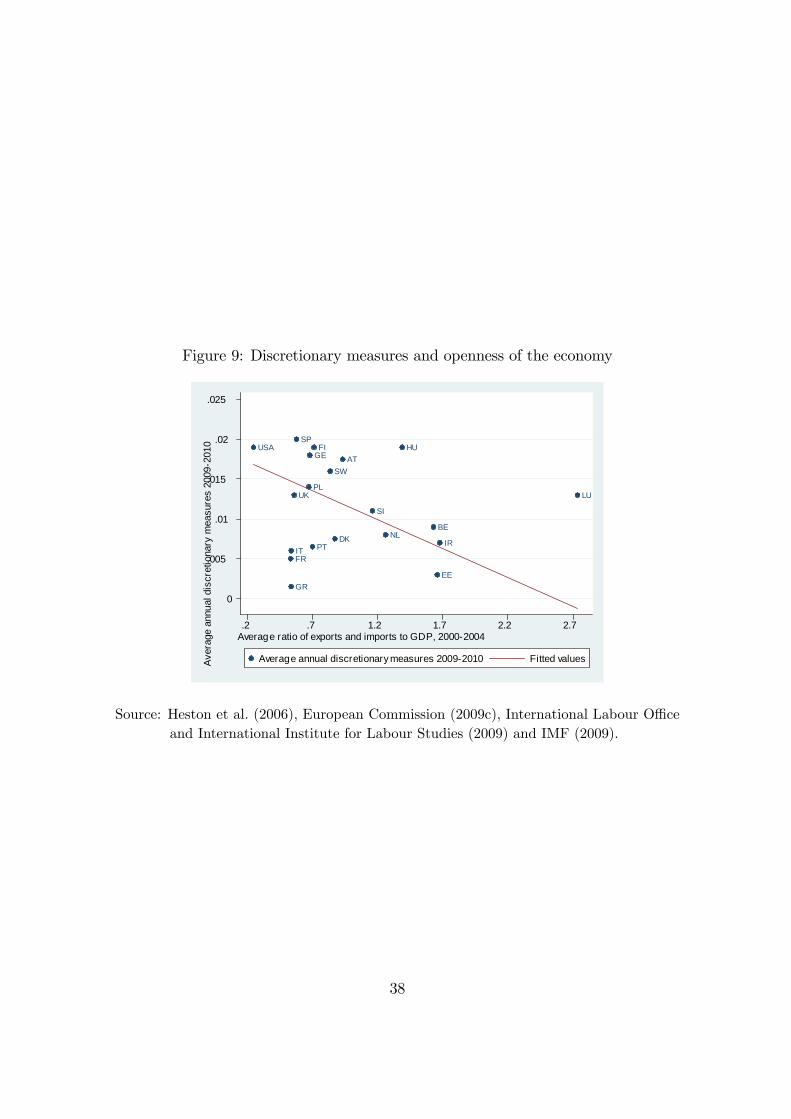
Figure 9: Discretionary measures and openness of the economy

AT

BEDK

EE

FI

FR

GE

GR

HU

IRIT

LU

NL

PL

PT

SI

SP

SW

UK

USA

0

.005

.01

.015

.02

.025

Aver

age 

annu

al d

iscr

etio

nary

 mea

sure

s 20

09­2

010

.2 .7 1.2 1.7 2.2 2.7Average ratio of exports and imports to GDP, 2000­2004

Average annual discretionary measures 2009­2010 Fitted values

Source: Heston et al. (2006), European Commission (2009c), International Labour O¢ ceand International Institute for Labour Studies (2009) and IMF (2009).

38

A.2 Reweighting procedure for increasing unemployment

In order to increase the unemployment rate while keeping the aggregate counts of

other key individual and household characteristics constant, we follow the approach

taken by Immvervoll et al. (2006). The increase of the unemployment rates is mod-

eled through reweighting of our samples while controlling for several individual and

household characteristics that determine the risk of becoming unemployed.

We follow Immvervoll et al. (2006) and de�ne the unemployed as people aged

19�59 declaring themselves to be out of work and looking for a job. The within-

database national �unemployment rate�is calculated as the ratio of these unemployed

to those in the labor force, de�ned as the unemployed plus people aged 19�59 who

are (self)employed. The increased total number of unemployed people is calculated

such that total household income decreases by 5% within each country.

In EUROMOD, the baseline household weights supplied with the national data-

bases have been calculated to adjust for sample design and/or di¤erential non-

response (see Sutherland (2001) for details). Weights are then recalculated using the

existing weights as a starting point, but (a) using the increased (decreased) num-

ber of unemployed (employed) people as the control totals for them, and (b) also

controlling for individual demographic and household composition variables using

the existing grossed-up totals for these categories as control totals. The speci�c

variables used as controls are:

� employment status

� age (0�18, 19�24, 25�49, 50�59, 60+)

� gender

� marital status and household size

� education

� region

This method implies that the households without any unemployed people that

are similar to households with unemployed people (according to the above variables)

will have their weights reduced. In other words, these are the households who are

�made unemployed�in our exercise.

39

References

Aaberge, R., Björklund, A., Jäntti, M., Pedersen, P. J., Smith, N. and Wennemo,

T. (2000). Unemployment Shocks and Income Distribution: How Did the

Nordic Countries Fare during Their Crises?, Scandinavian Journal of Eco-

nomics 102(1): 77�99.

Alesina, A. and Glaeser, E. (2004). Fighting Poverty in the U.S. and Europe: A

World of Di¤erence, Oxford University Press.

Alesina, A., Glaeser, E. and Sacerdote, B. (2005). Work and leisure in the U.S. and

Europe: Why so di¤erent?, NBER Macroeconomcis Annual pp. 1�64.

Andrés, J., Domenech, R. and Fatas, A. (2008). The stabilizing role of government

size, Journal of Economic Dynamics and Control 32: 571�593.

Auerbach, A. (2009). Implementing the New Fiscal Policy Activism, American

Economic Review: Papers and Proceedings 99:2: 543�549.

Auerbach, A. and Feenberg, D. (2000). The signi�cance of federal taxes as automatic

stabilizers, Journal of Economic Perspectives 14: 37�56.

Auerbach, A. and Hassett, K. (2002). Fiscal Policy and Uncertainty, International

Finance 5: 229�249.

Bargain, O. (2006). Microsimulation in action: policy analysis in Europe using

EUROMOD, vol. 25 of the series Research in Labor Economics, Elsevier.

Bayoumi, T. and Masson, P. (1995). Fiscal �ows in the United States and Canada:

Lessons for monetary union in Europe, European Economic Review 39: 253�274.

Bell, D. and Blanch�ower, D. (2009). What Should Be Done about Rising Unem-

ployment in the UK, IZA DP No. 4040.

Blanchard, O. (2006). Comments on �The Case Against the Case Against Discre-

tionary Policy�, by Alan Blinder, in R. Kopcke, G. Tootell and R. Triest (eds),

The macroeconomics of �scal policy, MIT Press, Boston, pp. 62�67.

40

Blanchard, O. and Perotti, R. (2002). An empirical characterization of the dynamic

e¤ects of changes in government spending and taxes on output, Quarterly Jour-

nal of Economics 117: 1329�1368.

Bourguignon, F. and Spadaro, A. (2006). Microsimulation as a tool for evaluating

redistribution policies, Journal of Economic Inequality 4(1): 77�106.

Buettner, T. and Fuest, C. (forthcoming). The Role of the Corporate Income Tax

as an Automatic Stabilizer, International Tax and Public Finance .

Buti, M. and van den Noord, P. (2004). Fiscal policy in emu: Rules, discretion and

political incentives, Moneda y Crédito 218: 265�319.

Cameron, D. (1978). The Expansion of the Public Economy: A Comparative Analy-

sis, American Political Science Review 72: 1243�1261.

Campbell, J. Y. and Mankiw, N. G. (1989). Consumption, income, and interest

rates: Reinterpreting the time series evidence, inO. J. Blanchard and S. Fischer

(eds), NBER Macroeconomics Annual 1989, MIT Press, p. 185½U216.

Devereux, M. and Fuest, C. (2009). Is the Corporation Tax an E¤ective Automatic

Stabilizer?, National Tax Journal LXII: 429�437.

Deville, J.-F. and Särndal, C.-E. (1992). Calibration estimators in survey sampling,

Journal of the American Statistical Association 87: 376�382.

DiNardo, J., Fortin, N. and Lemieux, T. (1996). Labor Market Institutions and the

Distribution of Wages, 1973-1992: A Semiparametric Approach, Econometrica

64: 1001�1044.

Eaton, J. and Rosen, H. (1980). Optimal redistributive taxation and uncertainty,

Quarterly Journal of Economics 95: 357�364.

European Commission (2009a). Public Finances in EMU 2009. 10th edition.

European Commission (2009b). Taxation trends in the European Union - 2009

edition.

European Commission (2009c). The EU�s response to support the real economy

during the economic crisis: an overview of Member States�recovery measures.

41

Fatàs, A. and Mihov, I. (2001). Government size and automatic stabilizers, Journal

of International Economics 55: 3�28.

Fatàs, A. and Mihov, I. (2002). The e¤ects of �scal policy on consumption and

employment: Theory and evidence, mimeo, INSEAD.

Feenberg, D. R. and Coutts, E. (1993). An Introduction to the TAXSIM Model,,

Journal of Policy Analysis and Management 12(1): 189�194.

Galí, J. (1994). Government size and macroeconomic stability, European Economic

Review 38: 117�132.

Galí, J., López-Salido, J. D. and Vallés, J. (2007). Understanding the e¤ects of

government spending on consumption, Journal of the European Economic As-

sociation March 5(1): 227�270.

Girouard, N. and André, C. (2005). Measuring cyclically-adjusted budget balances

for OECD countries, OECD Economics Department Working Papers.

Goode, R. (1976). The Individual Income Tax, revised edition, Brookings., Wash-

ington.

Herault, N. (2009). Sequential Linking of Computable General Equilibrium and Mi-

crosimulation Models, WP No. 2/09, Melbourne Institute of Applied Economic

and Social Research, The University of Melbourne.

Heston, A., Summers, R. and Aten, B. (2006). Penn World Table Version 6.2,

Center for International Comparisons of Production, Income and Prices at the

University of Pennsylvania.

IMF (2009). Group of Twenty - Global Economic Policies and Prospects, Note by

the Sta¤ of the International Monetary Fund.

Immervoll, H., Kleven, H., Kreiner, C. and Saez, E. (2007). Welfare Reform in

European Countries: A Micro-Simulation Analysis, The Economic Journal 117(516): 1�44.

Immvervoll, H. (2004). Average and marginal e¤ective tax rates facing workers

in the EU. A micro-level analysis of levels, distributions and driving factors,

EUROMOD Working Paper Series.

42

Immvervoll, H., Levy, H., Lietz, C., Mantovani, D. and Sutherland, H. (2006).

The sensitivity of poverty rates to macro-level changes in the European Union,

Cambridge Journal of Economics 30: 181�199.

International Labour O¢ ce and International Institute for Labour Studies (2009).

The �nancial and economic crisis: A decent work response.

Jappelli, T., Pischke, J.-S. and Souleles, N. (1998). Testing for Liquidity Constraints

in Euler Equations with Complementary Data Resources, Review of Economics

and Statistics 80: 251�262.

Jappelli, T. and Pistaferri, L. (forthcoming). The consumption response to income

changes, Annual Review of Economics .

Johnson, D., Parker, J. and Souleles, N. (2006). Household Expenditure and the

Income Tax Rebates of 2001, American Economic Review 96(5): 1589�1610.

Kleven, H. J. and Kreiner, C. (2006). The Marginal Cost of Public Funds in OECD

Countries: Hours of Work versus Labor Force Participation, Journal of Public

Economics 90: 1955�1973.

Mabbett, D. (2004). Fiscal Stabilisers In Europe: The Macroeconomic Impact Of

Tax and Bene�t Systems, EUROMOD Working Paper No. EM7/04.

Mabbett, D. and Schelkle, W. (2007). Bringing macroeconomics back into the po-

litical economy of reform: the Lisbon Agenda and the ��scal philosophy�of the

EU, Journal of Common Market Studies 45: 81�104.

McIntyre, R. S., Denk, R., Francis, N., Gardner, M., Gomaa, W., Hsu, F. and Sims,

R. (2003). Who pays? A Distributional Analysis of the Tax Systems in All 50

States, Institute on Taxation and Economic Policy.

Mélitz, J. and Zumer, F. (2002). Regional redistribution and stabilization by the

central governement in canada; france; the uk and the us: A reassessment and

new tests, Journal of Public Economics 86 (2): 263�286.

Parker, J. (1999). The Reaction of Household Consumption to Predictable Changes

in Social Security Taxes, American Economic Review 89 (4): 959�973.

43

Pechman, J. (1973). Responsiveness of the Federal Income Tax to Changes in In-

come, Brookings Papers on Economic Activitiy 2: 385�421.

Pechman, J. (1987). Federal Tax Policy, Brookings, Washington.

Perotti, R. (2002). Estimating the e¤ects of �scal policy in oecd countries, ECB

Working Paper No. 168.

Piketty, T. and Saez, E. (2007). How Progressive is the U.S. Federal Tax System?

A Historical and International Perspective, Journal of Economic Perspectives

21 (1): 3�24.

Prescott, E. C. (2004). Why do Americans work so much more than Europeans?,

Federal Reserve Bank of Minneapolis Quarterly Review 28 (1): 2�13.

Reinhart, C. and Rogo¤, K. (2009). The Aftermath of Financial Crisis, American

Economic Review: Papers & Proceedings 99 (2): 466�472.

Rodrik, D. (1998). Why Do More Open Economies Have Bigger Governments?,

Journal of Political Economy 106: 997�1032.

Runkle, D. (1991). Liquidity constraints and the permanent income hypothesis,

Journal of Monetary Economics 27: 73�98.

Sachs, J. and Sala-i Martin, X. (1992). Fiscal Federalism and Optimum Currency

Areas: Evidence for Europe from the United States, in M. B. Canzoneri, V.

Grilli and P. R. Masson editors, "Establishing a Central Bank: Issues in Europe

and Lessons from the U.S.", Cambridge University Press.

Saez, E. (2001). Using elasticities to derive optimal income tax rates, Review of

Economic Studies 68: 205�229.

Saez, E. (2002). Optimal income transfer programs: intensive versus extensive labor

supply responses, Quarterly Journal of Economics 117: 1039�1073.

Shapiro, M. D. and Slemrod, J. (1995). Consumer response to the timing of in-

come: Evidence from a change in tax withholding, American Economic Review

85(1): 274�283.

Shapiro, M. D. and Slemrod, J. (2003). Consumer response to tax rebates, American

Economic Review 93(1): 381�396.

44

Shapiro, M. D. and Slemrod, J. (2009). Did the 2008 tax rebates stimulate spending?,

American Economic Review: Papers & Proceedings 99(2): 374�379.

Souleles, N. (1999). The Response of Household Consumption to Income Tax Re-

funds, American Economic Review 89 (4): 947�958.

Sutherland, H. (2001). Final Report - EUROMOD: An Integrated European Bene�t-

Tax Model, EUROMOD Working Paper No. EM9/01.

Sutherland, H. (2007). Euromod: the tax-bene�t microsimulation model for the

European Union, in A. Gupta and A. Harding (eds), Modelling Our Future:

Population Ageing, Health and Aged Care, Vol. 16 of International Symposia in

Economic Theory and Econometrics, Elsevier, pp. 483�488.

van den Noord, P. (2000). The size and role of automatic stabilisers in the 1990s

and beyond, OECD Economics Department Working Papers, No.230.

Zeldes, S. (1989). Consumption and Liquidity Constraints: An Empirical Investiga-

tion, Journal of Political Economy 97 (2): 305�346.

45