NBER WORKING PAPER SERIES

INTERPRETING TESTS OF FORWARDDISCOUNT BIAS USING SURVEY DATAON EXCHANGE RATE EXPECTATIONS

Jeffrey A. Frankel

Kenneth A. Froot

Working Paper No. 1963

NATIONAL BUREAU OF ECONOMIC RESEARCH1050 Massachusetts Avenue

Cambridge, MA 02138June 1986

The research reported here is part of the NBER's research programin International Studies. Any opinions expressed are those of theauthors and not those of the National Bureau of Economic Research.

Working Paper #1963June 1986

Interpreting Tests of Forward Discount Bias UsingSurvey Data on Exchange Rate Expectations

ABSTRACT

Survey data on exchange rate expectations are used to dividethe forward discount into expected depreciation and a risk prem-iurn. Our starting point is the common test of whether the forwarddiscount is an unbiased predictor of future changes in the spotrate. We use the surveys to decompose the bias into a portionattributable to the risk premium and a portion attributable to sys-tematic prediction errors. The survey data suggest that ourfindings of both unconditional and conditional bias areoverwhelmingly due to systematic expectational errors. Regres-sions of future changes in the spot rate against the forwarddiscount do not yield insights into the sign, size or variability ofthe risk premium as is usually thought. We test directly thehypothesis of perfect substitutability, and find support for it inthat changes in the forward discount reflect, one for one, changesin expected depreciation. The "random-walk" view that expecteddepreciation is zero is thus rejected; expected depreciation iseven significantly more variable than the risk premium. In fact,investors would do better if they always reduced fractionally themagnitude of expected depreciation. This is the same result thatBilson and many others have found with forward market data, butnow it cannot be attributed to a risk premium.

Jeffrey A. Frankel Kenneth A. FrootDepartment of Economics Sloan School of ManagementUniversity of California MITBerkeley, CA 94720 Cambridge, MA 02139

Interpreting Tests of Forward Discount Bias Using

Survey Data on Exchange Rate Expectations

Kenneth A. .Proot

Sloan School of Management

Massachusetts Institute of Technology

Cambridge. Massachusetts 02139

Jeffrey A. Pranicel

Department of Economics

University of California, Berkeley

Berkeley, California 94720

1. INTRODUCTION

The forward exchange rate is surely the jack-of-all-trades of international

financial economics. Whenever researchers need a variable representing inves-

tor expectations of future spot rates, the forward rate is the first to come to

mind. On the other hand, the forward rate is frequently used to measure the

empirically elusive foreign exchange risk premium.

These two conflicting roles are most evident in the large literature testingwhether the forward discount is an unbiased predictor of the futurechange in

the spot exchange rate.1 Most of the studies that test the unbiasednessWe would like to thank Greg Connor and Toe Mattey for helpful comments, Barbara Bruer,John Calverley, Louise Cordova, Kathryn Dominguez, Laura Knoy, Stephen Marris, and PhilYoung for help in obtaining data, the National Science Foundation (under grant no. SES-8218300), the Institute for Business and Economic Research at U. C. Berkeley, and theAlfred P. Sloan Foundation's doctoral dissertation program for researchsupport.1 References include Tryon (19'?9), Lev-ich (1979), Bilsori (1981a), Longworth (1981)Hsieh (1982), Fama (1984), Huang (1984), Park (1984) and Hodrick and Srivastava (1986).For a recent survey of the literature and additional citations see Boothe and Longworth(1988).

-2-

hypothesis reject it, and they generally agree on the direction of bias. They

tend to disagree, however, about whether the bias is evidence of a risk premium

or of a violation of rational expectations. For example, studies by Longworth

(1981) and Bilson (1981a) assume that investors are risk neutral, so that the

systematic component of exchange rate changes in excess of the forward

discount is interpreted as evidence of a failure of rational expectations. On the

other hand, Hsieh (1984) and most others attribute the same systematic com-

ponent to a time-varying risk premium that separates the forward discount

from expected depreciation.

Investigations by Fama (1984) and Hodrick and Srivastava (1986) have

recently gone a step further, interpreting the bias not only as evidence of a risk

premium1 but also as evidence that the variance of the risk premium is greater

than the variance of expected depreciation. Bilson (1985) terms this view a new

"empirical paradigm" because it incorporates an essentially static model of

exchange rate expectations; changes in the forward discount predominantly

reflect changes in the risk premium rather than changes in expected deprecia-

tion. Often cited in support of this view is the work of Meese and RogofT (1983),

who find that a random walk model consistently forecasts future spot rates

better than alternative models, including the forward rate.

But one cannot address without additional information the basic issues of

whether systematic expectational errors or the risk premium are alone respon-

sible for the repeatedly biased forecasts of the forward discount (or whether it

is some combination of the two), let alone whether the risk premium is more

variable than expected depreciation. In this paper we use survey data on

exchange rate expectations in an attempt to help resolve these issues. The sur-

veys allow us to divide the forward discount into its two components - expected

depreciation and the risk premium -- and to inspect separately the properties

-3-

of each.

Though surveys of agents' expectations may in general be less desirable

than data on agents' actual market behavior, in this case the merit of a new

data source lies in what could not have been learned without it. One particular

advantage of the surveys is that our estimates of the risk premium do not

depend on the validity of any specific model or assumptions. As a consequence

we can test directly whether investors regard assets denominated in difTerent

currencies as perfect substitutes. A second advantage is that, with the issue of

the risk premium's existence tentatively resolved, we can then test the

hypothesis of forward rate unbiasedness and come away with a clear idea of

how much bias is due to the risk premium and how much is due to systematic

expeetational errors. A third advantage of the surveys (which cover a variety of

sample periods and forecast horizons) is that they can help us gain a sense for

the accuracy of earlier interpretations given to the large number of rejections

of the forward rate unbiasedness hypothesis.

The paper is organized as follows. Section 2 presents some simple descrip-

tive statistics from the survey data. Here the focus is primarily on the uncondi-

tional prediction errors of the forward discount. In section 3, we perform the

standard (conditional) test of forward discount unbiasedness, and use the sur-

veys to decompose the bias into a component attributable to systematic expec-

tational errors and a component attributable to the risk premium. In section 4,

we test formally whether the risk premium component is significantly different

from zero, that is, we test whether investors regard positions in different

currencies as perfect substitutes. In section 5, we test formally whether the

expectational errors component is significantly different from zero, that is, we

ask if the survey expectations are rational in the sense that they are formed in

a manner consistent with the true spot process. Finally. section 6 offers our

-4-

conclusions.

2. DESCRIPTIVE STATISTICS

Our exchange rate expectations data come from three independent sur-

veys. The first survey source is Money Market Services (MMS), Inc. Every two

weeks from January 1983 to October 1984, MMS spoke by phone with an average

of 30 currency traders or currency-room economists at major international

banks. Respondents were asked for their expectations of the value of the

pound, mark, Swiss franc and yen against the dollar in two weeks and three

months time. From October 1984 to February 1986, MMS conducted its survey

every week, asking for expectations one week and one month into the future.

The Economist Financial Report has conducted telephone interviews with

currency traders at 14 leading international banks one day each six weeks

beginning in June, 1981. On each occasion, respondents reported their expec-

tations of the value of the pound. French franc, mark, Swiss franc and yen at

three-, six- and twelve-month horizons. Finally, the Amex Bank Review (Amex)

surveys 250-300 central and private bankers, corporate treasurers and finance

directors, and economists, and records their expectations of the value of the

pound, French franc, mark, Swiss franc and yen against the dollar at six-month

and twelve-month horizons. Most of these data sets are discussed and analyzed

in Frankel and Froot (1986).2

Naturally, the benefits that survey data provide do not come without possi-

ble costs. The presence of heterogeneous beliefs, the use of the median

response, the lack of perfect synchronization, and the sheer volatility of the

spot rate all make some measurement error in the survey data likely. We

present results in section 4 which suggest that the surveys are surprisingly

2 Another paper that uses the MMS data is Dominguez (1988).

-5-

"clean". Nevertheless, we try to use only tests that are robust to the presenceof random measurement error in the data.3 In order to take advantage of the

complete sample of data available (the three sources contain over 1.450 data

points), we used every available opportunity to raise our sample sizes. The data

are frequently pooled across currencies. We also employ a method-of--moments

estimation procedure which allows us to pooi the data across different forecast

horizons.

2.1. Decomposition of ForwardRate Prediction Errors

The simplest test for whether the forward discount is an unbiased predic-tor of the future spot rate is a test for unconditional bias in the forward rateprediction errors. These errors are defined as:

— As ÷ = (f4— ,s'÷) + (s'— tst +) + (i)

where fd is the forward discount (the log of the current forward rate minus

the log of the current spot rate, f — s) expressed in terms of domesticcurrency, and and S+k are the log of the actual spot rate and expected

spot rate k periods into the future, respectively, minus the log of the current

spot rate. Equation (1) thus defines the risk premium, rp, as the expected

excess return required by investors in order to hold an open position in domes-

tic currency at time t and as the expectational prediction error, realized

at time t+k. If exchange rate risk is completely diversifiable and expectations

are rational, then the forward rate prediction errors should be purely random.4

Also, we experimented with different approximations to the precise survey and forecastdates of the Amex survey, which was conducted by mail over a period of up to a month. Weused the average of the 30 days during the survey and also the mid-point of the surveyperiod to construct reference sets. Both gave very similar results, so that only results fromthe former sample were reported.

Under perfect substitutability, expected real, and not nominal, profits should be zero;the two differ because of Jensen's inequality (see Engel, 1984). We do not incorporate theeffects of purchasing power uncertainty in this paper, however. One might expect theeffects are sma]l the standard deviation of unexpected changes in the inflation rate areabout 1/30 the size of the standard deviation in exchange rate changes (Litterman, 1980,and the results in Tables 1, 2 and 3 of this paper).

-6-

Table 1 reports the time series means of the forward discount, ex post

change in the spot rate and the forward rate prediction error in equation (1),

sampled on the days when surveys were conducted.5 In several cases (particu-

larly the MMS three-month data and the Economist and Amex twelve-month

data), we can reject the hypothesis that the forward rate is on average an

unbiased predictor of the future spot rate.6 The signs of the errors are clearly

sensitive to the sample period; they are negative in the later MMS sample

(October 1984 to February 1986) and in the Amex data from the late 1970s, but

positive in between. Columns (1) and (2) of Table 1 show that such variation is

due to substantial swings in average ex post exchange rate changes from sam-

ple period to sample period and not due to swings in the forward discount.

Without any additional information on investors' expected future spot rate,

one would have to assume that the risk premium is zero in order to inter-

pret equation (1) as a test of market efficiency. Alternatively, if one wishes to

interpret equation (1) as a test for the existence of a risk premium, the

assumption of rational expectations is required (i.e., ?7÷k is serially uncorre-ft ftlated and F? ( flg÷ft I Tg) = 0). Thus the results in Table 1 could be interpreted

as evidence that investors made repeated forecasting mistakes during some the

survey periods, .g that investors distinguished between assets denominated in

different currencies on the basis of risk (or else some combination of these

polar points of view).7b DEl provided us with daily forward and spot exchange rates, computed as the average

of the noon-time bid and ask rates.6 The Economist surveys, MMS one-month and three-month surveys, and the Amex

twelve-month survey were conducted at intervals shorter than their respective forecasthorizons. This implies that the prediction errors of the forward discount and of the surveyexpectations, in Tables 1 and 2 respectively, are not all independent, even under the hy-pothesis of rational expectations. For the Economist and MMS data, the standard deviationof the means were estimated by a method of moments procedure discussed in the followingsection. For the Amex data, confidence intervals were constructed assuming that thenumber of degrees of freedom is equal to the number of nonoverlapping observations. Thislatter procedure implies that t-tests reported for the Amex data are lower bounds.

7 Other potential candidates to explain the non-zero forward rate prediction errors arethe so-called "peso problem" (but see Frankel, 1985) and the convexity term due toJensen's inequality (see McCulloch, 1975).

—

P-.

, a-

(.

.I —

r— rn

C

UW

—4

.-*.

-'

—

- ..

Ci3

—

'-I

G3-

1.--

4 r

u r•

— i

-n

PiC

u—4

,-+

. —

' —

ni

— r

-i.,<

-4

c-.,

01

—'

._4 . 03

r c_

i ($3

13

Z

r

C..

•—l

Ct)

f -I

C

. ) ..

i-_

P.3

m

—I Il

l C

_. 0

, r-

—

rn

-4 rn

C

. ($3

=

a-

r 0-

v D

lb 1

QD

a-

C

O-V

rt

,,- -

ID

a-

i. i-li

3C

m

Cl

ZZ

• ((

3 —

4

x Ill

C

rn

fr_,

-1

rn

F) i , p_i

U)

ci,

01

Ct)

C

s)

0'.

—

0'.

0-—

-

01 ' -.J

— a

- Cs-

. 01

—

- -

. —

0) —.

4 --

4 —

a-

. C

s)

0-

'. c —

C

i —

—

'. 01

— 0

I 0)

— C

E

I —

a-

I $

I 0)

.-

I p.

- i 01

..C

U

(.4 4

0)

'—P

..3--

C

E

CE

I'J

- '—

p-.'-

0)

01

—

I'.3

.—

I..)

I P

..,

Ci

I C

-fl -'4

r.J

i 0)

0)

Li

i -.

. C

M--

4(M

z,

-

Cs,

Li

i -.

C

E

Lii

. 0)

0-

0)

-CU

01

0-

,_'_

U,

fl ri-

CU 0

C-,

- CI

rt,

rtfl'

I-

.. C

-Il ri

it, i,

Iii 0

.. rt

lb

r_

i ra

C

:3 -

, LII

g3.

0-rD

—

. C

U

—I

—

0-

-o .—

.. i-.

. ti

Pb

lb --

i °1

,n

Pb -

CI.—

- 0

it. n

3 -

' r'_

D E

-.

-. rr

o -—

rn

-s.

It. - r'_

C

U

Pt,

0-0

lb

— ra

'- CU 0

0-0

In

-<0 0

CU

P

b ci

ci

—4

I.n i-I

- .-C

PD

t3

:1

Pb

rt,

rt,

'4 r

. Ifi

Ui

—Q

,-

,. —

. CU

C

U

—. l

.n 0

.i P

3 P

u c-

.. -.

—

00

CU

C

.3 U

i —

Lfl

—.

—m

LL1

CU

1*

0

—.-

'_

U, 0

o-

00

CU

Ill

0

'.i

PD

C

U 0

0 r.

i 0.

. P

D

CU

o -,

i -

rDru

0 —

I..-

—

o

Lii

— p

:1

5 C

U

O lb

lb

SC

1 *

Lii

003

- Cs 0

lb 0

0-

t.3 a

- CU

-,

U' -

3 lb

•

C).

PC

i IV

' x -

.-

pCs

—I

—ci

U

i r*

4

so

0 r1

o

o-

0 o

fl r+

10

CU

P

D

r.

-,

PD

I_

' (C

I C

U

fl C

U

I-.-

-i lb

r..3

P..)

-CU

C

I)—

0—

,4 (.

4 V

.4 (

.4 (

.4 -

••_l

__(_

fl P

.) .'

f_Il

IJIQ

——

—

(.

4 (.

4 (.

4 (.

4 .4

0)

O—

00'-0

-Q-.

.C-

—

(.4

(.4

(.4 (4

-o

0101

0)C

EC

i —

.C

U .

.CU

01

JQ.-

..I-.

_j..4

—

-C

U C

U -C

U '-

J -.

.CU

.CU

..CU

0 —

C

U .C

U -C

U C

U (1

) --

40—

—..I

—-.

i—I

I'.,

a- a—

a- a

- .C

U

P'.)

.-1'

4P..)

'4

C.-

4 C

- I..)

$'4(

.40.

.

I C

M 0

-C

U . C-

P.)

l4(.

C-f

l --

,ICE

p..)

'C.p

...](

O

Csl

P

..)

—C

-Ci

I..)o

-. —

a

I -C

U 0

- -C

U -C

U C

i P..)

001,

..P.I(

4 c.

..a—

.CU

.-..s

o

i .C

U (4

1 -C

U L

i Ci p

...)

0--0

C...

.i._i

C-p

...)

—J-

.oo-

--n.

o--C

,

(-.1

a—

-CU

. (.4

0).—

a-(.

.1—

..4

cnp.

..j..,

,cj,

I —

c.-a

c.—

I c—

i —

0.

.4P

S.)

lIP

..)

CE

.CU

JIC

.4

0-C

EP

-.)

0) (3

) 0

a-C

-flP

'.)

I I

I I —

, I

C-E

M(.

—-.

oQ-

C. "

-a 0

- P..)

C

U .0

3 0)

C-f

lC-C

--..J

I-.)

P'.3

CE

(.rI

03

-.0

-ø

a-t3

)03

I I

I I

I (.

.-4C

iC-0

-Cs-

I..)

CM

,_..J

-a

P3

—.1

—

P..)

0-C

s--0

-OC

I3

I I

I —

Ci..

CU

a-

(.4

CU

U) -

03 .

CU

U)

P(.

.4(.

44

ii I

— —

— —

-J

C.ic

4Ci

-0 0—

0-

-0--

I P

..) p

.., P

..) —

P..)

—

c,IC

io

CM

-.

4 01

— 0

1 Li

iQ-.

P..3

(..4

$-..)

ii I

— .-

— —

C

U(.

4(41

0.-P

..)

P-.

—

— (-

1 (.

I0--

-OLf

lCJI

P..)

is.)

P..)

— P.

.)

-CU

Ci'.

*C-

(.4

— C—

I -.

0 I-

.)

-.0C

i0—

0--C

i

— U

C

i —1 C

' —

.-—

—

LI

I Ps.

) 30

-4

C. -

c ,

I C

i -.4

(.4

— a

. ii t.j

. .C

U

30 C

U (,

-4C

i 0—

V..4

—

——

.—

0 03

I III

P

.).—

r..—

——

-—

(—I-

-aC

- C

s) I-

.) -C

U

P..)

—C

-(.-

I'IO

Li

i C--

i I-.

) C

) - C

i P

-.)-

C-Ø

a—

-j P..)

(.4(

.,—,—

.03

— .

-J It

.- C

M C

i CE

(.

-ILI

I(.ii

,n(,

.$30

C

- P..)

Lii -

(3 .

.J C

U

-J'-.

.1C

-4p.

,)L

fl

LII - a

-- -a

—

Lii . iO

(.4-

0 E

X)C

iLii.

.C3I

Ji

CE

p..,

-a

--a

I -.

01.3

30

.lP'.3

(.4C

-.I

II C

ip-.

3 C

i•C-C

i O

CiC

iC,C

-Ci

C.IC

--Ic

,40-

lii

i .0

3(...

IC-

P.3

0—

P..)

a-

'—Jp

-—I-

.)p.

.,(3)

(.

4 C

-fl C

i (.1

P..)

Lii

C.c

3)Lf

l 0-

....a

C

i P

..3i0

a)(.

..I.C

i P

..JP

- C

M .0

3 P

..) 0

C

_Il —

C-i -o

-03

—

-CU

-c03

C)C

---I

P

.) (

-1 C

M .0

- P

,.),—

—p.

C

...lo

-o3,

.-..,

—

—

— —

a.

—

—

— —

—

— —

—

—

—

—

—

— —

— —

a.

— —

—

—.4

—

—

-Il

—m

"'I

C,

I 0:

1:.

alt',

C-3

m

rn. O

I —

II m

i C

r31

ID

U, 0 'l-

U, 0'

I,-

03

-D

0 -4 —$1

-.

0 lb

-ii

0

r,

—4

lb

CU

0 '

-am

lb

-I

Ca'

03

o z

0 Cs

15

'—--

C

Cs)

-4

-I

01

—

4

C-,

01

I -'-

.0

I —

—1

I l0

P..)

I

Lii

I ..+

-40)

I"' —

:15-

-I--

I —

—

I 10

3CU

—

In m

l—

-0-n

- m

Lfl

I —

'010

1---

P

S-

— 4s

.)

÷

01'-

—m

c-,

Cs,

—4

-7-

In Table 2 we use the survey data to separate the forward rate prediction

errors into the two terms on the right-hand-side of equation (1): the risk prem-

ium and expectational errors. Here the conclusions concerning the nature of

each are surprisingly very different from those one might draw from Table 1.

Note first that the means of the risk premia measured in the survey data are

large, averaging around an annualized 5 percent and reaching 9 percent in

several cases. Second, and perhaps even more striking, is that nothing about

the sign or magnitude of the risk premia as measured by the survey data can be

inferred from the forward discount prediction errors. In fact, the premia in

column (1) of Table 2 happen to be consistently opposite in sign from the for-

ward rate errors.6 Third, the risk prernia often appear negatively correlated

with the forward rate errors, not just across data sets, but within each data set

as well. The first column of Table 3 reports correlation coefficients for each

currency and survey: 21 of the 33 estimates are less than zero. Charts 1

through 4 show the time series of the forward rate errors and the survey risk

prernia for each of the data sets.9 The graphs show how badly the forward pred-

iction errors have measured the premia in the past.

Such a poor correspondence might suggest instead that the survey data

are very imprecise measures of investors' true expectations. But, in the first

place, it should be noted that findings of unconditional bias are unaffected by

any measurement error in the survey data, provided the error is random. Posi-

tive and negative measurement errors should tend to cancel out, just as posi-

tive and negative prediction errors should tend to cancel out under the null

hypothesis. In the second place, we offer an explicit estimate of the magnitude

This is the same as saying that the survey prediction errors are of the same sign as theforward rate errors, but have consistently larger absolute values.

° Graphs 1-3 use moving averages across all of the currencies included in the designatedsurvey. The Amex data in Graph 4 were straightforward averages over the five currenciessurveyed.

I— •

1 '-

a-

(--I

—

1.4

—

ID

1 N

.)

U.'

'D

CD

-

__

__

4 DII

44-i

rn

fl

-fl-

u.

—

4 —4

—I

—4

—4

—I

—I

—4 rn

—I rn

r In •

—

r— r'

-i .-

., E

n '1

14=

r'

rn

c_. U

') "l,

4=

—

4 —

. U

, 'T

i 4=

—

. Cl)

4=

—

4 a—

. ES

) 4=

'—

4 C

— (5

) 4=

..

()

4=

Cc.

C

: P1 Cc. '-i

U

) I'c

-_4

—4

P1 . —

4 ) 'c

—'I rn

—

U) " —

4 C

) —

4 C

) 7 —4

C

) Cl —

4 U

) (7)

—I

'1

cr1 I_c.

,4-'1 _

_ —

Zr

1-4-

'1

S fl

I C

D

rt

' i)

C

D —

1Cn

CD —

r—

r-

r-

C

C

).-4

- '1

-.<

44

-,)

I_c.

ID'C)'1=i

'Oa

IDC)-a

mID

C) -,

U.'

-, -,

'1

-,

- ID

--,

a-'1

a

C)

C)

C)

C.)

o

1 C).. a

a-

a.

— C:

0 C

D

al/I

' -4

. i,

-—

C)

rn

rn

rn

. -

('1

C")

-—

r.,n

U

,)

C)

U

24-

Zr

2).

Zr

_ C

) C

) C

) —

C: CD C)

441

Cl,

CS)

(I

) L

I)

Cl)

—

II

4-4-

L

X)

U)

- - -

: 4

—I

-

rt.r

__

1I=

__lc

fl

Ifl ct

-,

—

a-

- —

a-

. 0'

. —

—

—

—

rd

-i

1

CS

--'.—

--.-

a--'.

.—

---.

—

. —

..-

-".

4=4

=4

—rd

ID

'--

—-I

'-'.-

, ')'

) "—

—

rnl .

CO

C

O

CO

'-.

E

D

—..

.4-

''-<

IX

I U

— '.

4 C

D 0

- ''-I

c-

—

I,

,-I

CD

(.

4 0)

4,

—

0-

I 0-

I

I I

I Ic

—I

."—

II

—

—

I —

—

- In

— -,

C

XI

I-Z

l (0

1—.)

C

D I.

.) C

D

1-4

N.)

C

) 4-

.)

C)

1.4

.1:,

cC' I1

C

D

— -

-..-

. ".

'--

".

- '._

'-—

'-'..

'-...

'-—

"-

'-'-.

'..

'a

CXI..J(0

CD

IZX

I-.J

CD

0)

0)

C

D

CO

C

O

CD

—

. I_fl

ID

,-.-

(34 CD CM

CJI

c-

fl U

) c-n

c-

n c-

n -P

1 0'

—

-

a-.

'-P1

—

(Ii

—'-I

_fl

I,)

4-'-

—

—

4,,)

I

CII

'1

P44.

4P1

(-,4

(1.'4

(-'4

ç.40

4-

31.4

(34

c-4(

-4(.

.ic-.

4C,4

0)

J(.4

c-,1

.0

P144

--P1

.P1C

O

P1-

P1,

P1"

.J

-P1-

P1.

P1.

CO

(7

'-O.-

a-Q

--..P

1 C

l -'l

- -C

:- 0— U'-

c-fl

c-Il 0—

—

0—

12

— 0

— 0'

- 0'

- -C

:. C

O C

OE

D 0

) CD

-C:-

—

,I 0

- -'.4

'---

4—I

.P1

P1 ..P

1 - 0-

- '.4

0— '-

.4 '.

4 —

4 4-

4 —

4,,)

4,,) -.4

rI

-' C

c, &n r'C

fl

-•I'

fl rd

C

:P1

I I

1114

I

Ii,

1111

11

1111

11

1111

1,

I a-

((I

(-.4

— C

) 0—

- '-4 '

-.1 --i c

-n

c--i -C:- —

CD

0- C

D C

O P

1 '-.

4 '-.

40'- '

-4 .0

c--i

a—

-P1

c--I

l:4 ,P

1 -

— (

..i c

-Si C

O (.

4 —

ID

—

Ii

C::

— 0

- ( 0-—

C)

.-0

c--i

(Xl

c-n

— C

O

(-'4

- -4 -D

I-,)

4-4

'-0

.-l —

P1 —

'.4

-.0

CD

.P1

a-- C

) C)

(-—

I C

) - C

D

fl I,)

4-

3-.i'

.4

(.-I

C)-

C:-

C).

P1c-

'I - .P

11

.P1C).C:--.P1r-—I,4

—0CO,—I.3p'., N).OEMCO'

--.9-00--0--

CMt4-C)P1

—

Ifl —

I'.C

C

: I

I

I

I

I I

II I

I I

I 4

c-.c

--IN

.)

III

1—--lP-4

1114 I

c-.. 4I I

I

) .4'C) CD

C)'-—'.

LnC

)W"—

iLJI

CO

c-

flC

)c--

i (M

-DC

.-.I

-P10

'-c-f

l 0-

a-

0C..i

c-.i

—Jc

--1c

JI--

,4C

) C

)—I'-

-r-.

,,c-.

l C

).

a.

0 J4'4

4-4 0'- ,

4-c X

I - —

'-J —

* - '-0

C) —

.-i '

-0

(.-I

---.

J-0

c--i C

) 0'-

c-fl c-

n C

.-I 0

- -0

a- 4,

,) 4-

.) c

-n C

) C:

I.J..—.--i)

Lfl—GCX)O'-c-.IC.4

-0-4

.0

C)CO,CDQ-.P1

-'4C)-C)0---P1-o

'—JI---.-DI-.)CO

CD-P1CJ1COCM

2)-

CD

Ui

CD'1

-

— —

— — —

— — — — — — —

— — — — — — — — — — —

— ——

—

— —

4.____

— —. —

— —

—

— —

— —

—

— —

-,

E

LI in

—

*

— —

— —

—

—

—

— —

- —

— —

—

— —

— —

—

— —

— —

—

— —

0"--

rD

"—C

D

IlIl.n

I,)a.

. (b

Lfl

Lfl

O

—

CD

Ifl ,+

'l P1

1110

i

I I

I I

I I

- ,4-

' ID

— I

I I

— —

—

—

—

—

—

4-4 —

— 0-

—4C

M c

--i .

P1

,—I —

.4-,

,)

.0 4

3(.-

4 —

.—- —

C

O -C

) —D

C- .

4)

—P

-) 1-3 C

OE

D

-P1.

—. 0

— P

-3(,

--I

1.3.

0 C) c

--I a

- C

D.—

. C

D

In P

IO)

—0

cC'

-4

C) —

4

c-n "-

I — '-

-4 C

D

'.4 -

4 .-

—

-.4 '.4 c-Cl C

' cI -4

N.) 12

) cC

:. C

S- C) -.

0

c-n I

j-,) C

- c--

I c-f

l c-

n C

- C) C

) - a-

-0 N.

) 4.

(-C

l .0

Nj c

-n —

—I —

C

D

U4

I_fl

C

)c-I

I -.

0(--

IN,)

C-C

..i(-

-i -0

CD

* a-

-.Ja

--C

Dp-

.4C

:.'

'-OLX

I4-4

—'-0

'-.J

CO

c-.4

CD

c--4

'--

4-00

,).P

1-4-

. c-

-ic-n

CO

-.o-

--4

-.0—

4N)-

o'--

J 4,

P

1 — -

=4 a

CD

"'

-I

__ II

1111

11

11

C-

c-.1L34 c-n - -

- —

—

—

—

—

—

— —

c-

fl (

01-3

—

.j c-

-i _n

.. CD c.

-i .4

--

CD 0— '-

—4 - (X

I -01

2--a

- -0

c--I

—.4

—

.4 c

-n a

- —4 - —

,I '--

-4 -

0 '.4

—

CD

(-'I

—C

I -P1

0) '-O

C) C

) '.1

('Q

c 0-

C)

F.)

(--lCD — (J

i c-n c

.,i -.

0 a-

(4

C/ic

-fl

4-30

- EDP.) c-n c

-n

c--I

c--

Ia- -

P1—

c--i

—00

) 1-.

.I(JI

N.)

0-

0- C)

-P1-I

'.4 c

-lI C

. C. -

0 0-

-.0

c--I

-c—

—

—

—. —

— — — —

—

— _f

a —

— — — — —

— — — —

— — * —

—

— —

— — — — — —

*

— _

— —

—

— —

— — _

—-4.

— — — — ..

—

— — — —

U,

4=

Cl,

— --C

I-

fl C)

-v 24-

CD

-

-I —

4-

• —4

CDU) P1

0 — x

—

CD

-4

-' 54

- C

D N)

-' '-C

P

1 CI)

=4

—4

=4

C: '—I

Cl)

—4

C')

U)

rn-a

u'

m

— 'C

:'

—--44= —

— V

P'-)

C

) I Zr 441

U'

-C

rn

I-I- l

'4.

XI

— -U

-I

C)

rn

14-

+ rn

—

- 4=

rn-i

, C

) C)

4444

1

Zr U)

—4

CI)

Ci)

cC:

-a

C'1

rn

rn —<

C)

—4

I,,

LI)

Zr rl UI

PS

rt

-

CD

P1

=4

1-C'

UI

1-C'

CI.

1-

4-I

CDI

P1

I

0

I

I -o

U

I (I

) —

1-4-

+

II II

— I

-

I I

-'-c-

C

- -.I Ci-

c-n N..) -

'3-C

: '-0

C) —

1 (-

.1

.—O

'- c-fl 4-

3 -.

.j -P

1 C

) .P

1 c-

-i

0— (

-.1

0--E

DO

) -

C/i C

O C

) c--

i —0

(--4

.0 C

) N.) — C

- N.J (

--4 C)'

1-3 -.0.0

.P1 (--4

(-.1 —

—

(.4C

M CM

c-.

'. :,

N.)

c-,

CD

-C:-

C/i —

0 c-

n C

ON

.) -

c-fl

c--I

P.,)

Ci.

-CC

) 0-

c-iC

-.)

— '—

4 0-

-C/I

C) CD

C) c-n -,o

—-.

i -

(.,fl

.n. (

S—

-0

C) N

j-C C

D-0

-8-

of this measurement error component in section 4. In the third place, the

degree to which the surveys qualitatively corroborate one another is striking.

For example, the risk premium in the Economist data (Chart 1) is negative dur-

ing the entire sample, except for a short period from late 1984 until mid-1985.

The MMS three-month sample (Chart 2) reports that the risk premium did not

become positive until the last quarter of 1984, while MMS one-month data

(Chart 3) shows the risk premium then remained positive until mid-1985. That

the surveys agree on the nature and timing of major swings in the risk premium

is some evidence that the particularities of each group of respondents do not

influence the results.

We can test whether the data statistically reject the hypothesis that the

means of the forward rate prediction errors are attributable entirely to the risk

premia alone, assuming that the surveys measure expectations accurately. The

tests for the significance of the mean survey prediction errors in Table 2 show

that 27 out of 44 samples reject the hypothesis that the survey expectations

are unbiased predictors of the future spot rate. This is a rejection of the

equivalent hypothesis that the systematic component of the forward rate pred-

iction errors is attributable entirely to the risk premium. We can also test

whether the data statistically reject the hypothesis that the errors are attri-

butable entirely to the existence of expectational errors. Table 2 shows that we

can easily reject this hypothesis because the risk premium is significantly

different from zero and of the opposite sign.

The survey data therefore suggest that an interpretation of the uncondi-

tional bias in the forward rate prediction errors that imposes rational expecta-

tions would lead to consistently incorrect conclusions with respect to the sign

of the risk premium and the nature of its time-series variation. At the opposite

extreme, the systematic portion of the errors could be interpreted solely as evi-

Ii

V

V

FORWARD605040302010

0—10'I—20

—30

—40

-50—60

—70

—80

—90

—10024—Oct—84

RATE ERRORS & THE RISK PREMIUM

0 Forward Rate Error - p.,l,-

CHART 1

FORWARD RATE ERRORS & THE RISK PREMIUM3 MONTH ECONOMIST SURVEY DATA SMOOTHED30

20

10

0

—10

—20

—30

—4023—Jun—81 01 —Jun—82 09—May—83 16—Apr—84 19—Mar—85

D Forward rate error + Risk Premium

CHART 3

1 MONTH MMS SURVEY DATA SMOOTHED

27—Feb—85 10—Ju1—8 04—Dec—85

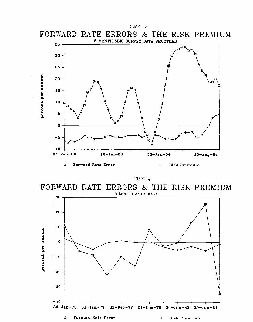
CHART 2

FORWARD RATE ERRORS & THE RISK PREMIUM3 MONTH MMS SURVEY DATA SMOOTHED

I

35

30

25

20

15

10

5

0

—5

—1005—Jan—83

Q Forward Rate Error

CHART 4

+ R15k Premium

FORWARD RATE ERRORS & THE RISK PREMIUM6 MONTH AMEX DATA

04

C)

04

30

18—Jul—83 30—Jan—84 15—Aug—84

20

10

0

—10

—20

—30

—40

30 —Jan—76

0 Forward Rate Error + Riuk Prmj,irr

31—Jan—77 01—Dec—77 01—Dec—78 30—Jun—82 29—Jun—84

-9-

dence of a failure of rational expectations, but then the forward rate errors

would offer no evidence at all regarding the substantial risk premia recorded in

the survey data. Either interpretation, or any combination of the two, would

miss the fact that the survey risk premium lies in the direction opposite to that

indicated by the results in Table 1, that is, expectational errors are more than

100 percent responsible for the unconditional bias in the forward rate errors.

2.2. Variability of the Risk Premium andExchange Rate Expectations

Survey data can also be used to shed some Light on the relative volatility of

expected depreciation and the risk premium. The recent papers by Fama

(1984) and Hodrick and Srivastava (1986) argue that the risk premium is more

variable than expected depreciation or, in the extreme formulation of Bilson

(1965), that expected depreciation is zero. Table 3 shows the variance of

expected changes in the spot rate and the variance of the risk premia, for each

data set and broken down by currency. The magnitude of ex post exchange

rate changes (column (1)) dwarfs that of the forward discount (column (2)).10

For example, the reported variance of annualized spot rate changes of 2 per-cent represents a standard deviation of about 14 percent. By comparison, the

variance of expected depreciation is around .25 percent. a standard deviation

of 5 percent.

The variance of expected depreciation is comparable in size to the vari-

ance of the risk premium, and is larger in 36 of the 40 samples calculated in

Table 3. Thus "random walk" expectations are do not appear to be supported

by the survey data. We test formally the Fama (1984) hypothesis that the vari-

ance of expected depreciation is less than the variance of the risk premium in

section 4. Both are several times larger than the variance of the forward

10 This empirical regularity has often been noted; e.g., Mussa (1979),

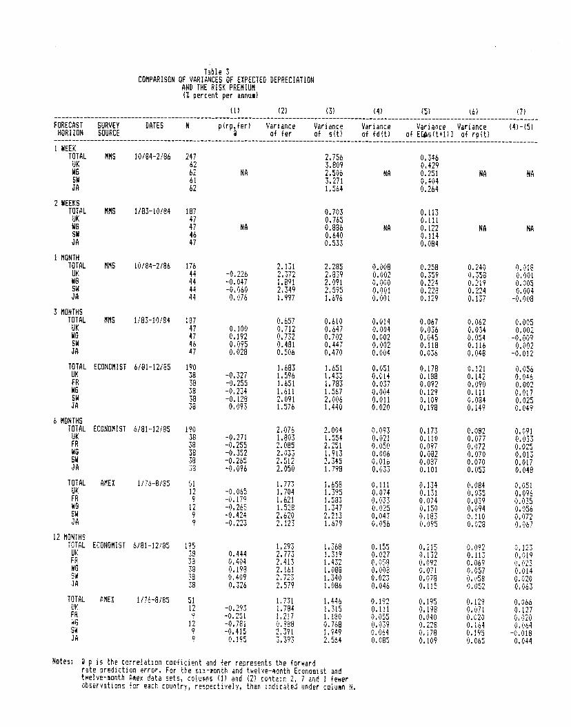
Table 3CUIPARIGON OF VARIAIICU OF EXPECTED DEPRECiATION

All TIE RISK PREIIIUIIii percent per anna)

(1) (2) (3) (4) (5) (6) (7)

FORECASTHORIZON

SURVEY DATESSOURCE

N p(rp far) Varianceof far

Yarianceof nit)

Varianceof Hit)

Varianceof EIts(t+1)l

Varianceof rp(t)

(4)—IS)

1HOEKTOTAL 181$ 10/84-2/Oh 247 2.756 0.346

UK 62 3.809 0.429HO 62 NA 2.506 NA 0.251 NASN 61 3.271 0.404

62 1.564 0.264

2 HOEKSTOTAL 181$ 1183—10184 187 0.703 0.113It 47 0.765 0.11188 47 NA 0.886 NA 0.122 NA NASN 46 0.640 0.114lA 47 0.533 0.084

innTOTAL 181$ 10/84—2186 116 2.131 2.285 0.008 0.258 0.240 0.018It 44 4.226 2.372 2.839 0.002 0.359 0.358 0.001ND 44 4.047 1.891 2.091 0.000 0.224 0.2*9 0.005SN 44 4.060 2.349 2.595 0.001 0.228 0.224 0.004U 44 0.076 1.997 1.696 0.001 0.129 0.137 4.008

3 NOIITHS

TOTAL 181$ 1/83—10184 *87 0.657 0.610 0.014 0.067 0.062 0.005It 41 0.100 0.712 0.647 0.004 0.036 0.034 0.002ND 47 0.192 0.732 0.702 0.002 0.045 0.054 4.009SI 46 0.095 0.481 0.447 0.002 0.118 0.116 0.002U 47 0.028 0.506 0.470 0.004 0.036 0.048 4.012

TOTAL ECONONIST 6/81—12/85 190 1.683 1.651 0.051 0.178 0.121 0.056It 38 4.327 1.596 1.433 0.014 0.188 0.142 0.046FR 38 4.255 1.651 1.783 0.037 0.092 0.090 0.00288 38 4.234 1.611 1.567 0.004 0.129 0.111 0.011511 38 4.128 2.091 2.006 0.011 0.109 0.084 0.025lA 38 0.093 1.576 1.440 0.020 0.198 0.149 0.049

6 MONTHSTOTAL ECONWIIST 6/81—12/85 190 2.016 2.004 0.093 0.173 0.082 0.091UK 38 4.27! 1.803 1.554 0.02* 0.110 0.077 0.033FR 38 4.255 2.085 2.251 0.050 0.097 0.072 0.025ND 38 4.352 2.033 1.913 0.006 0.082 0.070 0.013SN 38 4.265 2.512 2.345 0.016 0.087 0.070 0.011U 38 4.096 2.050 1.798 0.033 0.101 0.053 0.048

TOTAL AMEX 1/16-8/85 51 1.773 1.658 0.111 0.134 0.084 0.051It 12 4.065 1.704 1.395 0.074 0.131 0.035 0.096FR 9 4.179 1.621 1.583 0.033 0.074 0.039 0.035HO 12 4.265 1.528 1.341 0.025 0.150 0.094 0.056SN 9 4.424 2.620 2.213 0.043 0.183 0.110 0.072lA 9 4.223 2.123 1.679 0.056 0.095 0.028 0.067.

12 MONThSTOTAL ECIIINNIIST 6/81—12/85 195 1.293 1.368 0.155 0.215 0.092 0.123It 38 0.444 2.773 1.319 0.027 0.132 0.113 0.019FR 38 0.404 2.413 1.432 0.058 0.092 0.069 0.023HO 38 0.198 2.161 1.088 0.008 0.071 0.057 0.014SN 38 0.409 2.723 1.340 0.023 0.078 0.058 0.020U 38 0.326 2.579 1.086 0.046 0.115 0.052 0.063

TOTAL AlEX 1/16-0/85 51 1.731 1.446 0.192 0.195 0.129 0.066It 12 4.293 1.784 1.315 0.111 0.198 0.071 0.127FR 9 4.251 1.211 1.180 0.055 0.040 0.020 0.02088 12 4.181 0.988 0.768 0.039 0.228 0.164 0.064SN 9 4.415 2.391 1.949 0.064 0.178 0.195 4.018U 9 0.195 3.393 2.564 0.085 0.109 0.065 0.044

Notesa 3 p is the correlation coeficient and far represents the forwardrite prediction error. For the siz—eonth and twelve—sooth Econosist andtwelve—sooth Ann data sets, cabins (11 and (2) contain 2, 1 and I fewerobservations for each country, respectively, than indicated uatdr coluan N.

- 10 -

discount. Thus the relative stability of the forward discount masks greater

variability in its two components, corroborating Fama's finding that the risk

premium is negatively correlated with the expected change in the spot rate11

Table 3 also has implications for tests of serial correlation in the forward

rate errors, fcL — LSg4ft. Such tests have been performed by Hansen and

Hodrick (1980), Dooley and Shafer (1982) and others. Under the assumption of

rational expectations, any serially correlated component of the forward rate

errors would be evidence of a time-varying risk premium. However, the small

size of the variance of the risk premium compared to the variance of the for-

ward rate errors (reported in columns (2) and (6) of Table 3, respectively),

implies that even when the null hypothesis of no serial correlation fails because

of the risk premium such tests will have low power. Using the assumption of

rational expectations and equation (i), the autocorrelation coefficient of— t+k converges in probability to:

ft ft ftCOV(Dpg ,rpg_ft) var(rp)

ft p — (i')var(fdg — ESg ÷) var(fd — ts-fk)

where p is the probability limit of the corresponding autocorrelation coefficient

of the risk premium. Table 3 suggests that ratio of the variance of the risk

premium to that of the forward rate errors on the righthand-side of equation

(1') has an upper bound of 0.1.12 Thus, even if the the risk premium follows a

random walk, so that p = 1, this ratio implies that the upper bound for the por-

tion of the autocorrelation coefficient of the prediction errors attributable to

This correlation is, however, biased downward by any measurement error that mightbe present in the surveys. If such error is purely random, theniie cnxariance of expectedderecietjoijnd the risk premium may be written as cov(s,+ft,rpt) —var(÷k), where3L+k and rpt are the "true" values of expected depreciation and of the risk premium,respectively, and E+k is the measurement error component of the survey.

1 In the Economist data for example, the autocorrelation coefficient of the survey riskpremium p, is considerably less than one: for the three-, six- and twelve-month data sets pequals .19, .23 and .08, respectively.

- 11 -

the risk premium is only 0.1.

3. USING THE SURVEY DATA IN THE FORWARD RATE UNBIASEDNE5S REGRESSION

In tests of forward market unbiasedness, attention has focused on the

optimal weights placed on the forward rate versus the contemporaneous spot

rate in predicting the future spot rate. The equation most commonly used is a

regression of the future change in the spot rate on the forward discount:

k k= a ÷ pfd + tt+k (2)

where the null hypothesis is that the weight on the forward rate is one and the

constant term is zero, i.e., fi = 1 and a = 0. In other words, the realized spot

rate is equal to the forward rate plus a purely random error term. A second but

equivalent specification is a regression of the forward rate prediction error on

the forward discount:

— = a1 + + tlt+k (2')

where a1 = —a and = 1—fl. The null hypothesis is now that a1 = fl1 = 0: theleft-hand-side variable is purely random.

Most tests of equation (2) have rejected the null hypothesis, finding fi to be

significantly less than one. The range of point estimates has been wide, from

about -2.8 to 0.8. Coefficients that are positive, but less than one, imply that

the optimal predictor of the spot rate puts positive weight on both the forward

rate and the contemporaneous spot rate. A coefficient of zero is the random

walk hypothesis: the forward discount is of no help in forecasting future spotrate changes.13 Least appealing, but nevertheless not unusual, are findings of

' Findings of this kind are not limited to investigations of foreign exchange markets. Intheir study of the expectations hypothesis of the term structure, for example, Shiller,Campbell and Schoertholts (1983) conclude that changes in the premium paid on longer-term bills over short-term bills are useless for predicting future changes in short-term in-terest rates,

- 12 -

significant negative coefficients, which indicate that the spot rate tends to move

in the direction opposite to that predicted by the forward discount.

As in the previous section, tests of equation (2) are joint tests of rational

expectations and no exchange risk premiuim Without other information, how-

ever, researchers have been forced to focus on one alternative hypothesis at

the expense of the other. For example, one could ignore the risk premium and

interpret the forward rate as representing investors' expectations. In this con-

text, Bilson (1981b) proposed that the alternative of less than one be termed

"excessive speculation", because it would imply that investors could do better

on average if they were to reduce fractionally their forecasts of exchange rate

changes, and that the alternative of f? greater than one be termed "insufficient

speculation", because it would imply that investors could do better if they were

to raise multiplicatively the magnitude of their forecasts of exchange rate

changes.

The most popular alternative hypothesis in regressions of equations like

(2), however, is that domestic and foreign securities are imperfect substitutes

because of risk. As we have already mentioned, Fama (1984), Hodrick and

Srivastava (1985) and Bilson (1985) argue that coefficients close to zero in such

regressions can be viewed as evidence of a risk premium that, is more variable

than are expectations. By taking probability limits, the slope coefficient in

equation (2) can be rewritten as:

k kcov(tsg÷k,fdg) cov(I.s÷k,fd)=

var(fd) var(Es÷k) + 2cov(s:÷,i,) + var(rp)

var(ts÷k) + cov(ts÷k,rp)________— — —- (3)var(ts÷k) + 2cov(s+k,rp7) + var(rp)

where the second equality follows from assuming rational expectations. If <

- 13 -

as is usually found, it follows that var(rp) > var(Es÷k). Accordingly, Bilson

(1985 p. 63) interprets the accumulated results of such regressions as evidence

that "most of the variation in the [forward] premium reflects variation in the

risk premium rather than variation in the expected rate of appreciation."

Indeed, the growing body of evidence that is insignificantly different from zero

does not permit one to reject the extreme view that expectations are totallyunrelated to the forward rate, in other words, that all variation in the forward

discount is attributable solely to variation in the risk premium.

3.1. Econometric Issues

Before turning to our own estimates of equation (2). we pause briefly to

mention several important econometric issues.

Estimation of equation (2) (and most of the equations we estimate later), is

performed using OLS. We stack different countries, and in some cases different

forecast horizons, into a single equation. The complicated correlation patternof the residuals, however, renders the OLS standard errors incorrect in finite

samples. Several types of correlation are present.

First, there is serial correlation induced by a sampling interval shorter

than the corresponding forecast horizon (up to eight times). This is the usual

case in which overlapping ob .vations imply that, under the null hypothesis,

the error term is a moving average process of an order equal to the frequency

of sampling interval divided by the frequency of the horizon, minus one. Han-

sen and Hodrick (1980) propose using a method of moments (MoM) estimatorfor the standard errors in precisely the application studied here.

Second, in order to take advantage of the fact that the surveys coveredfour or five currencies simultaneously, we pooled the regressions across coun-tries. This type of pooling induces contemporaneous correlation in the residu-

- 14 -

als.14 Normally. Seemingly Unrelated Regressions should be used to exploit this

correlation efficiently. We use SUR later; here, however, the serial correlation

induced by overlapping observations makes SUR inconsistent.

The basic model may be written as:

k k k=t-k .P + v (4)

where k is the number of periods in the forecast horizon and i indexes the

currency. We account for the two types of correlation in the residuals with a

MoM estimate of the covariance matrix of :

= (4')

where is the matrix of regressors of size N (countries) times T (time). The

(i,j)th element of the unrestricted covariance matrix, ci is:

=1

E E gj7g_17 for n=0,. ,N—1NT—k

= 0 otherwise. (5)

where r is the order of the MA process, is the OLS residual, and k = li—i

In some cases, this unrestricted estimate of C) uses well over 100 degrees of

freedom.15 We therefore estimated a restricted covariance matrix, C) with typi-cal element:

N1

(t+iT. f—k +pT) = E c,(t+1T, f—k +pT) if A =p and —r � k � rN—i

N-iN-I2

= E E w(t +It, t—k+pT) if andN(N—1) p=Oi=O

14 Each currency in our pooled regressions was given its own constant term. This model-3flg sta-ategy seemed most reasonable in view of the dilTerences across currencies in themagnitudes of both ex post spot rate changes and the forward discount (see Table 1).

15 The number of independent parameters in the covariance matrix does not affect theasymptotic covariance, as long as these rarameters are estimated consistently (see Hansen

- 15 -

= 0 otherwise (6)

These restrictions have the effect of averaging the own-currency and cross-

currency autocorrelation functions of the OLS residuals, respectively, bringing

the number of independent covariance parameters down to 2r.

Tests of forward discount unbiasedness also provide an opportunity to

aggregate across different forecast horizons (though we are unaware of anyone

who has done this, even with the standard forward discount data), adding a

third pattern of correlation in the residuals. Such stacking seems appropriate

in this case because we wish to study the predictive power of the forward

discount generally, rather than at any particular time horizon. Moreover, a

MoM estimator which incorporates several forecast horizons has appeal beyond

the particular application studied here because it is computationally simpler

than competing techniques and at the same time can be more efficient than sin-

gle k-step-ahead forecasting equations estimated with MoM.

To demonstrate the precise nature of the correlation induced by such

aggregation, consider the stochastic process, , which is stationary and

ergodic in first differences and has finite second moments. We denote the k

period change in y from period f—k to t as y, and the h period change asn-i

= where h = nk for any positive integer n16 We then define the=0

innovations, v and as:

k k kv =Y —E(yj (7)

(1982)). Nevertheless, one suspects that the small-sample properties of the MoM estimatorworsen as the number of nuisance parameters to be estimated increases,

16 The following example can easily be generalized to allow h and k to be any positiveintegers. It is also possible to combine iii a similar fashion more than two diflerent forecasthorizons. Indeed, we combine three horizons in the Economist data estimates in the regres-sions below. Because these extensions yield no additional insights and come at the cost ofmore complicated algebra, however, we retain the simple example above.

- 16 -

h h= Yg — E( y pt—h)

where includes present and lagged values of the vector of right-hand-sidevariables, z. These facts allow us to write the covariance matrix of the innova-

tions as:

k kv 11k hE = F [v'v'] = [ , h (6)

where the (i,j)th element of each submtrix of E is equal to the correspondingautocovariance function, evaluated at q = i —

= E( VtV+q) = if 1 q I <k (9)= 0 otherwise,

tSjE(l1g?VI+g)Xqhif qcZh= 0 otherwise

=E(VL/g'+g)=Xqif0�q<k (10)= E( v14'q) = if —h <q <0

= 0 otherwise

In this context consider the aggregated model:

y=xtP4-Vt (ii)where Yg' [y÷ Y+h'1' z' [zr' x] and [v' V7+h'J. The OLS estimate

of then has the usual MoM estimate of the sample covariance matrix:

—1 —1a = (x2NTx2NT) xEx(xx)

where is a consistent estimate of E, and is formed by using the OLS residuals

to estimate the autocovariance and crosscovariance functions in equations (9)and (10).

One might think that by stacking forecast horizons, as we do in equation

(ii), greater asymptotic efficiency always results than if only the shorter-term

- 17 -

forecasts are used, in other words, that — 2 is positive semidefinite. After

all, the sample size has doubled, and the only additional estimates we require

are nuisance parameters of the covariance matrix. This intuition would be

correct for asymptotically efficient estimation strategies, such as maximum

likelihood. But because OLS weights each observation equally, the MoM covari-

ance estimates reflect the average precision of the data. it follows that if the

longer-term forecasts are sufficiently imprecise relative to the shorter-term

forecasts, the precision of the estimate of fi drops: we could actually jefficiency by adding more data. In the appendix we demonstrate this potential

loss in asymptotic efficiency, and show how it is related to the disparity in fore-

cast horizons. Efficiency is most likely to increase if the longer-term forecast

horizon is a relatively small multiple of the shorter-term horizon, indeed, in the

forthcoming regressions we find a marked increase in precision from stacking

across forecast horizons when r = 2 (in the Economist and Amex samples), but

little or no increase in precision when r = 4 or 6 (in the MMS samples).

Finally, the above MoM estimates of the covariance matrix need not be

positive definite in small samples. Newey and West (1985) offer a corrected esti-

mate of the covariance matrix that discounts the jth order autocovariance by

1 — (ji(,n+1)), making the covariance matrix positive definite in finite sample.

Nevertheless, for any given sample size, there remains the question of how small

in must be to guarantee positive definiteness. In the upcoming regressions we

tried in = r (which Newey and West themselves suggest) and in = 2r; we report

standard errors using the latter value of in because they were consistently

larger than those using the former.17

17 For the two aggregated MMS data sets in Table 8 below, a value of in = r was usedafter finding that in = 2r resulted in a nonpositive semi-definite covariance matrix Thiscorrection reduced the standard errors in these two regressions by an average of only 3percent.

- 18 -

32. Results

Table 4 presents the standard forward discount unbiasedness regressions

(equation (2)) for our sample periods.18 Most of the coefficients fall into the

range reported by previous studies. Note that in the Economist and Amex data

sets, in which forecasts horizons were stacked, the standard errors fell in the

aggregated regressions by 14 and 31 percent, respectively, in comparison with

regressions that used the shorter-term predictions alone. In terms of the point

estimates, all but one of the data sets indicate that the optimal predictor of the

future spot rate places negative weight on the forward rate, and more than half

of the coefficients are significantly less than zero. There is ample evidence to

reject unbiasedness. In the two MMS data sets, which cover shorter sample

periods of 14 and 21 months, respectively, the coefficients have unusually large

absolute values, lending support to the observation by Gregory and McCurdy

(1984) that the regression relation in equation (2) may be unstable. The F-tests

also indicate that the unbiasedness hypothesis fails in most of the data sets.

At this point, we could interpret the results as reflecting systematic pred-

iction errors. Under this interpretation, it follows that agents would do better

by placing more weight on the contemporaneous spot rate and less weight on

other factors in forming predictions of the future spot rate, the view discussed

by Bilson (1981b). On the other hand, we could interpret the results as evi-

dence of a time-varying risk premium. Then the conclusions would be that

changes in expected depreciation are not correlated (or are negatively corre-

lated) with changes in the forward discount and, from equation (3), that the

variance of the risk premium is greater than the variance of expected deprecia-

tion.

Regressions were estimated with dummies for each country, which we do not report tosave space. For the regressions which pool over different forecast horizons (markedEconomist Data and Amex Data), each country was allowed its own constant term foreveryforecast horizon.

TABLE 4

TESTS OF FORWARD DISCOuNT UNBIASEDNESS

IlLS Regressions of ésIt+I) on fd(t)

Ftes$DataSet Dates I t:Iso t:S'i Il OF tsO,Bui frob)F

Econosist Data 6181—1218.5 —0.5684 —0.56 —1.54 0.16 509 2.12 0.007

(1.0171)

Econ 3 Month 6/81—12185 -1.2090 -1.04 -1.91 S 0.01 184 1.29 0.262(1.1596)

Econ 6 Month 6181—12185 —1.9819 —1.37 —2.06 5* 0.07 174 1.47 0.191

(1.4445)

Econ 12 Month 6/81—12185 0.2892 0.23 —0.56 0.29 149 3.23 0.005

(1.2733)

WAS 1 Month 10/84—2186 —14.5529 —2.43 *5 —2.59 5* 0.21 171 2.67 0.024

16.0000)

WAS 3 Month 1183-10/84 —6.2540 —2.91 *5* —3.37 *1* 0.50 183 12.01 0.000(2.1508)

AMEX Data 1/76—7/85 —2.2107 —2.30 *5 —3.34 *1* 0.23 86 2.60 0.007

(0.9623)

AMEX 6 Month 1/76—7/85 —2.4181 —1.92 * —2.71 *5* 0.26 45 2.42 0.041

(1.2608)

AMEX 12 Month 1/76—7185 —2.1377 —2.03 5* —2.97 *5* 0.21 40 1.66 0.157

(1.0549)

Notes: Method of Moeents standard errors are in parentheses. $ Represents significance at the

102 level, 5$ and *1* represent significance at the 52 and IX levels, respectively.

- 19 -

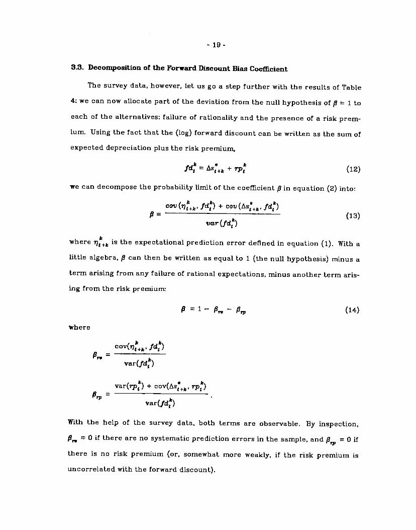
3.3. Decomposition ot the Forward Discount Bias Coefficient

The survey data, however, let us go a step further with the results of Table

4: we can now allocate part of the deviation from the null hypothesis of = 1 to

each of the alternatives: failure of rationality and the presence of a risk prem-

ium. Using the fact that the (log) forward discount can be written as the sum of

expected depreciation plus the risk premiurn,

ft e ftfd = + rpg (12)

we can decompose the probability limit of the coefficient in equation (2) into:

ft ft ftcov(rlg÷k,fdt) + COV(fSft,fdg)

9= (13)ftvar(fd)

where is the expectational prediction error defined in equation (1). With a

little algebra, can then be written as equal to 1 (the null hypothesis) minus a

term arising from any failure of rational expectations, minus another term aris-

ing from the risk premium:

(14)

where

ft ftcov(flft, fd)

—

var(fd)

var(rp) ÷ cov(Lsft. i-p)ft

var(fd)

With the help of the survey data, both terms are observable. By inspection,= 0 if there are no systematic prediction errors in the sample, and = 0 if

there is no risk premium (or, somewhat more weakly, if the risk premium is

uncorrelated with the forward discount).

- 20 -

The results of the decomposition are reported in Table 5a. First, ,8, is very

large in size when compared to ,, often by more than an order of magnitude.

In all of the regressions, the lion's share of the deviation from the null

hypothesis consists of systematic expectational errors. For example, in the

Economist data, our largest survey sample with 525 observations, = 1.49 and= 0.08. Second, while is greater than zero in all cases, is sometimes

negative, implying in equation (14) that the effect of the survey risk premium is

to push the estimate of the standard coefficient in the direction above one. In

these cases, the risk premia do not explain a positive share of the forward

discount's bias. The positive values for , on the other hand, suggest the pos-

sibility that investors tended to overreact to other information, in the sense

that respondents might have improved their forecasting by placing more weight

on the contemporaneous spot rate and less weight on the forward rate. Third,

to the extent that the surveys are from different sources and cover different

periods of time, they provide independent information, rendering their agree-

ment on the relative importance and sign of the expectational errors all the

more forceful. To check if the level of aggregation in Table 5a is hiding impor-

tant diversity across currencies, Table Sb reports the decomposition for each

currency in every data set. Here the results are the same: expectational errors

are consistently large and pusitive, and the risk premium appears to explain no

positive portion of the bias.

While the qualitative results above are of interest, we would like to know

whether they are statistically significant, whether we can formally reject the

two obvious polar hypotheses: a) that the results in Table 4 are attributable

entirely to expectational errors; and b) that they are attributable entirely to

the presence of the risk premium in the survey data. We test these hypotheses

in turn in the following sections.

TABLE Se

COIPSIENTS OF TIE FAILURE OF THE UIIBIASEDNESS HYPOTHESIS

IN REGRESSIONS OFASItt1) ON FD(t)

Failure of Existence of IspliedRational RIO Prenixe Regression

Expectations Coefficient(1) (2) 1—(1)—(2)

Approxmnate *Data Set Bates N 8, B

Econoalst Data 6/81-12185 525 1.49 0.08 -0.57

Econ 3 Month 6/81—12/85 190 2.51 -0.30 —1.21

Econ 6 Month 6181—12/85 180 2.99 0.00 —1.98

Econ 12 Month 6/81—12/85 155 0.52 0.19 0.29

IllS I Month 10184—2186 176 15.39 0.16 —14.55

III 3 Month 1183—10/84 188 6.07 1.18 —6.25

AMEX Data 1176-7185 97 3.25 -0.03 —2.21

AlEX 6 Month 1/76—7185 51 3.63 -0.fl —2.42

AlEX 12 Month 1/76—7184 46 3.11 0.03 —2.14

TABLE Sb

COMPONENTS OF TIE FAILIME OF THE UNBIASEDNESS HYPOTHESIS

IN REGRESSIONS OFAS(t+1) ON FD(t)

Failure of Existence of I.pliedRational Risk Preulus Regression

Expectations Coefficient

(1) (2) 1—(1)—(2)

ApproxianteData Set Dates N

#'rc

A

BjipI

WON 3 MONTH 6/81-1 2/85 190 2.51 —0.30 —1.21It 38 7.31 —1.11 —5.20FR 38 —1.75 0.47 2.28II 38 7.69 —1.64 -5.05SN 38 5.03 —0.63 —3.40IA 38 4.66 —0.73 —2.93

WON 6 MONTH 6(81-12/85 180 2.99 0.00 -1.98UK 36 7.04 —0.17 —5.87

FR 36 —1.31 0.21 2.10VS 36 10.16 -0.38 —8.77

50 36 5.75 -0.01 -4.74

IA 36 4.69 -0.18 —3.51

WON 12 MONTH 6/81-12/85 155 0.52 0.19 0.29UK 31 1.87 0.93 —1.79FR 31 —1.45 0.16 2.29

MO 31 —0.13 0.16 0.96

SN 31 0.96 0.25 —0.21IA 31 3.09 —0.04 -2.05

MIS 1 MONTH 10/84—2/86 176 15.39 0.16 -14.55UK 44 21.23 0.06 -20.28US 44 10.34 -8.95 -0.3958 44 13.15 —2.89 —9.26IA 44 4.58 7.10 -10.68

MIS 3 MONTH 1(83—10/84 188 6.07 1.18 6.25UK 47 7.90 0.27 —7.16MO 47 4.96 2.52 —6.48SN 47 7.90 0.09 —6.90IA 47 3.43 2.14 —4.57

AMEX 6 MONTH 1/76—7/85 51 3.63 —0.22 —2.42UK 12 2.76 —0.15 —1.60FR 9 1.09 —0.03 —0.06US 12 4.78 —0.63 —3.15SN 9 5.53 -0.33 —4.20IA 9 4.58 —0.10 —3.48

NIX 12 MONTH 1(76—7/84 46 3.11 0.03 2.14UK 11 2.53 —0.09 —1.45FR 8 0.48 0.32

VS 11 3.53 —0.40 —2.13SW 8 3.99 0.38 —3.37IA 8 5.36 0.12 —4.49

- 21 -

4. A Direct Test of Perfect Substitutability

We consider first a test of whether the bias introduced by the risk prem-

ium. p,,. is statistically significant. The most direct test is a regression of the

survey expected depreciation against the forward discount:

= a2 + 2fd + e2g (17)

where the null hypothesis is that no risk premium separates the two, a2 = 0 and

= 1. Strictly speaking, the expected future spot rate exactly equals the for-

ward rate if assets are perfect substitutes, so that we should interpret the

regression error as measurement error in the surveys. Thus,

= iS + 2t' where t+k is the unobservable "true" market expected

change in the spot rate. Note that if the null hypothesis holds, we can use the

R2 from equation (17) to obtain an estimate of the relative importance of the

measurement error component in the survey data.19

To see that a test of = 1 is equivalent to a test of = 0, note that the

OLS estimate of converges in probability to:

s kvar(rpt) + cov(As1+rp)

(18)var(fd)

= 1 —

k.where rp is the survey risk premium less any measurement error, i.e., the

"true" market risk premium, fd — Equation (17) may also be used to test

formally the Fama (1984) hypothesis regarding the size of the variance of

expected depreciation relative to the variance of the risk premium. A little

algebra yields:' Note also that in a test of equation (17) using the survey data, the properties of theerror term, 2 will be invariant to any "peso problems," which affect instead the ex postdistribution oTactuel spot rate changes.

- 22 -

—kvar(s+k) — var(rp)

P2 = i———— + . (19)var(fd)

Equation (19) says that if p2 is significantly greater than , the variance of

expected depreciation exceeds that of the risk prerriium. The qualitative

finding in Table 3, column (6). that the variance of expected depreciation is the

greater can thus be tested formally. Although measurement error in the survey

data would tend to overstate both of these variances, it does not affect the esti-

mate of their difference (equation (19)). This point is evident from equation

(17), in which the measurement error e2 is conditionally independent of the

estimate of as long as it is random, i.e., E(2g fd) = 0.

Under mild assumptions, equation (17) may also be interpreted as a direct

test of uncovered interest parity. If we rule out the presence of riskiess arbi-

trage opportunities, then by covered interest parity the forward discount

exactly equals the excess return paid on domestic securities relative to foreign

securities:

.k .k k— ?'' = fd

where and are the domestic and foreign interest rates on instruments

which mature in k periods. Uncovered interest parity is thus the hypothesis

that the interest differential equivalent to investors' expectations of future

depreciation.20

4.1. Results

Table 6 reports the OLS regressions of equation (17). In some respects the

data provide evidence in favor of perfect substitutability. All of the estimates of

are statistically indistinguishable from one (with the sole exception of the

° For tests of uncovered interest parity similar to the tests of conditional bias in theforward discount that we considered in section 3, see Cumby and Obstfeld (1981).

TULE 6TESTS SF PWEC1 SUSSTITIJTUILITY

01.5 Regrnuions if Es(t+1)] on fd(t)

F testlutaSet Pates I ts1.5 tilel R IF IN asO,11 Prob)F

Ecouoeist Pita 6181—12185 0.9880 3.33 $14 4.08 0.89 554 1.44 28.61 0.000(0.1465)

ka 3 Mouth 6181—12185 1.3037 3.14 *1* 1.19 0.10 184 1.56 16.55 0.000

(0.2557)

Ecou 6 Mouth 6/81—12185 1.0326 3.14 4*1 0.19 0.89 184 1.37 52.06 0.000(0.1694)

Econ 12 Mouth 6/81—12185 0.9286 2.86 *1* 4.48 0.91 184 1.44 65.82 0.000(0.1499)

MM8 I Month 10/84—2/86 0.1416 0.20 —0.09 0.21 171 1.02 6.79 0.000(1.fl75)

853 Month 1/83—10/84 4. 1816 —1.59 —2.75 1*1 0.73 182 1.50 14.60 0.000(0.4293)

ME! Pita 1/76—7185 0.9605 1.85 * 4.16 0.64 91 0.74 5.38 0.000(0.2495)

ME! 6 Mouth 1/76—7/85 1.2165 3.44 14$ 1.04 0.71 45 1.45 6.32 0.000(0.2085)

AlE! 12 Mouth 1/76—7/85 0.8770 1.37 4.45 0.61 45 0.51 8.10 0.000(0.2755)

Motes: Method of Mouents staudurd errors are in parentheses. I Represents siguificance at the102 level, $1 and *1* represent significance at the 52 aid 12 levels, respectively.

- 23 -

MMS three-month sample). In the Economist and Amex data sets which aggre-

gate across time horizons, the estimates are 0.99 and 0.96, respectively.21

Expectations seem to move very strongly with the forward rate. With the excep-tion of the MMS data, the coefficients are estimated with surprising precision.

As we might expect, however, the large magnitudes of the riskpremia discussed

in section 2 cause us to reject perfect substitutability. Each of the F-tests

reported in Table 6 rejects the parity relation at a level of significance that is

less than 0.1 percent.

In terms of our decomposition of the forward discount bias coefficient,

Table 6 shows the values of j9,., in column 2 of Table 5a are not significantly

different from zero. Thus the rejection of unbiasedness found in the previous

section cannot be explained entirely by the risk premium at any reasonable

level of confidence. Indeed, in spite of the fact that the survey risk premium

has substantial magnitude (Table 2), we cannot reject the hypothesis that the

risk premium explains no positive portion of the bias.

Table 6 also reports a t-test of the hypothesis that = }. In six out of

nine cases the data strongly reject the hypothesis that the variance of the truerisk premium is greater than or equal to that of true expected depreciation; we

have rather var(ACk) > var(). In addition, equation (16) and the findingthat = 1 together imply that:

Thvar(rp) + cov(Asrp) = 0

Thus we cannot reject the hypothesis that the covariance of true expected

depreciation and the true risk premium is negative (as Fama found), nor can we21 For the Economist six-month and twelve-month and the Amex twelve-month data sets,the estimates of ft2 from equation (1?) do not exactly correspond to 1 — ft in Tables ba

and 5b, This is because Table 6 includes a few survey observations for whicffactual futurespot rates have not yet been realized, whereas these observations were left out of thedecomposition in Tables 5a and 5b for purposes of comparability. If we had used the small-er samples in Table 6, the regression coefficients would have been .92 and 1,03, for theEconomist and Amex data sets, respectively.

- 24 -

reject the extreme hypothesis that the variance of the true risk premium is

zero.

2, -Note that the R s in Table 6 are relatively high. Under the null hypothesis

that true expected depreciation exactly equals the forward discount, one could

interpret these results as evidence that the measurement-error component of

the survey data is relatively small. For example, under this interpretation of

the statistics, measurement error accounts for about 10 percent of the vari-

ability in expected depreciation from the Economist survey.22 The presence of a

time-varying risk premium uncorrelated with the forward discount, however.

implies that the disturbance term, will riot be purely measurement error

but will also include variation of the risk premium around its mean. In this case

a second interpretation of the R2 measure is possible: that it overstates the

measurement error component of the surveys. Indeed, the low values of the

Durbin-Watson statistics reported in Table 6 seem to suggest the presence in

the OLS residuals of a risk premium which is serially correlated but uncorre-

lated with the forward discount.

In Table 7 we correct for the potential serial correlation problem by

employing a Three-Stage-Least-Squares estimator that allows for contem-

poraneous correlation (SUR) as well as first order auto-regressive distur-

bances.23 3SLS is consistent here because there are no overlapping observa-

tions -- predictions by the forward rate and the surveys are observed contem-

poraneously -- and it has the advantage of being asymptotically efficient. The

results reported in Table 7 show that this correction does not change the

nature of the results; all but one of the coefficients remain close to one, and

Recall, however, that the Ff2 measures in Table 6 include the explanatory power of theconstant terms for each currency and forecast horizon.

Unfortunately, the highly irregular spacing of the Amex data sets did not permit anauto-regressive correction in this case.

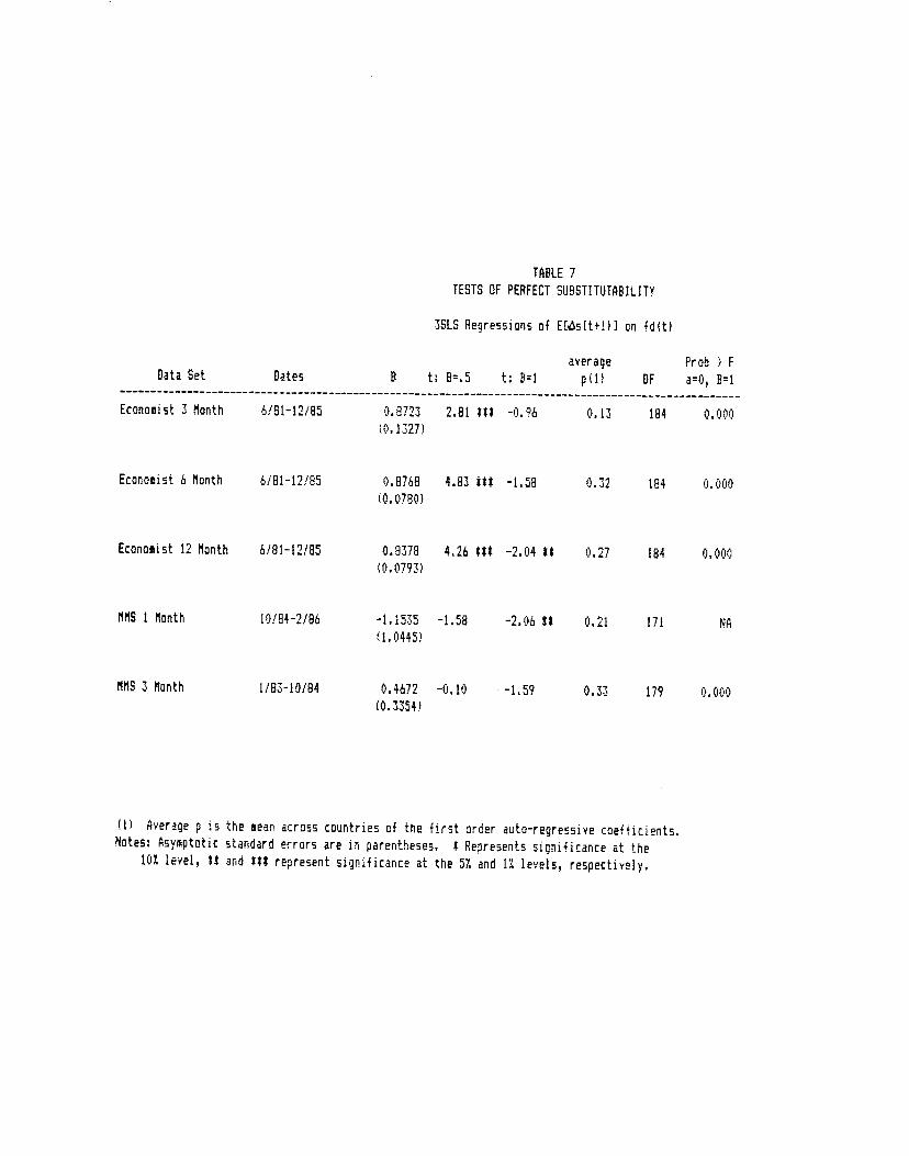
TABLE 7

TESTS OF PERFECT SUBSTITUTABILITY

3518 Reqressions of ErsIt+1)] on +d(t}

average Prob > FData Set Dates B t B.5 t: 8:1 p(l> OF a:0, 8:1

Economist 3 Month 6/81—12/85 0.8723 2.81 U$ -0.96 0.13 184 0.000

tO.1327)

Economist 6 Month 6181—12/85 0.8768 4.83 UI —1.58 0.32 184 0.000

(0.0780)

Economist 12 Month 6/81—12/85 0.8378 4.26 $11 —2.04 1$ 0.27 184 0.000

(0.0793)

MMS I Month 10164—2/86 —1.1535 -1.58 -2.06 II 0.21 171 NA

U. 0445)

MMS 3 Month 1/83-10/84 0.4672 —0.10 —1.59 0.33 179 0.000

(0.3354)

(1) Average p is the mean across countries of the first order auto—regressive coefficients.

Notes: Asymptotic standard errors are jr parentheses. * Represents significance at the

lOX level, *1 and *1* represent significance at the 57. and 17. levels, respectively.

- 25 -

there is clear evidence that the variance of expected depreciation is greater

than that of the risk premium (while there is no evidence for the alternative

that the variance of the risk premium is greater).

5. Tests of Rational Expectations

In this section we test to see whether the interpretation of the standard

bias findings in section 3 as evidence of systematic prediction errors can be

supported. While in section 2 we found evidence that investors err in their

unconditional forecasts of future changes in the spot rate, here we focus

instead on whether investors tend to place too little weight on the contem-

poraneous spot rate and too much on all other information. Tests of rational

expectations which address this question typically regress future prediction

errors of the forward discount on subsets of the contemporaneous information

set. As we have already noted, these tests are only valid in the absence of a risk

premium.. Consequently, we use here the prediction errors of the survey data

instead.

5.1. A Test of Excessive Speculation

Perhaps the most powerful test of rational expectations is one which asks

whether investors would do better if they placed more or less weight on the

contemporaneous spot rate as opposed to .fl other variables in their informa-

tion set.24 This test is performed by a regression of the expectational prediction

error on expected depreciation:

— = a + + Vt+k (20)

where the null hypothesis is a = 0 and d = 0.25 This is the equation that Bilson

Frankel and Froot (1986) test whether the survey expectations place too little weighton the contemporaneous spot rate and too much weight on specific pieces of informationsuch as the lagged spot rate, the long-run equilibrium exchange rate, and the lagged ex-pected spot rate.

To see how the alternative in equation (20)is too much or too little weight on all vari-ables in the information set other than the contemporaneous spot rate, assume expecta-

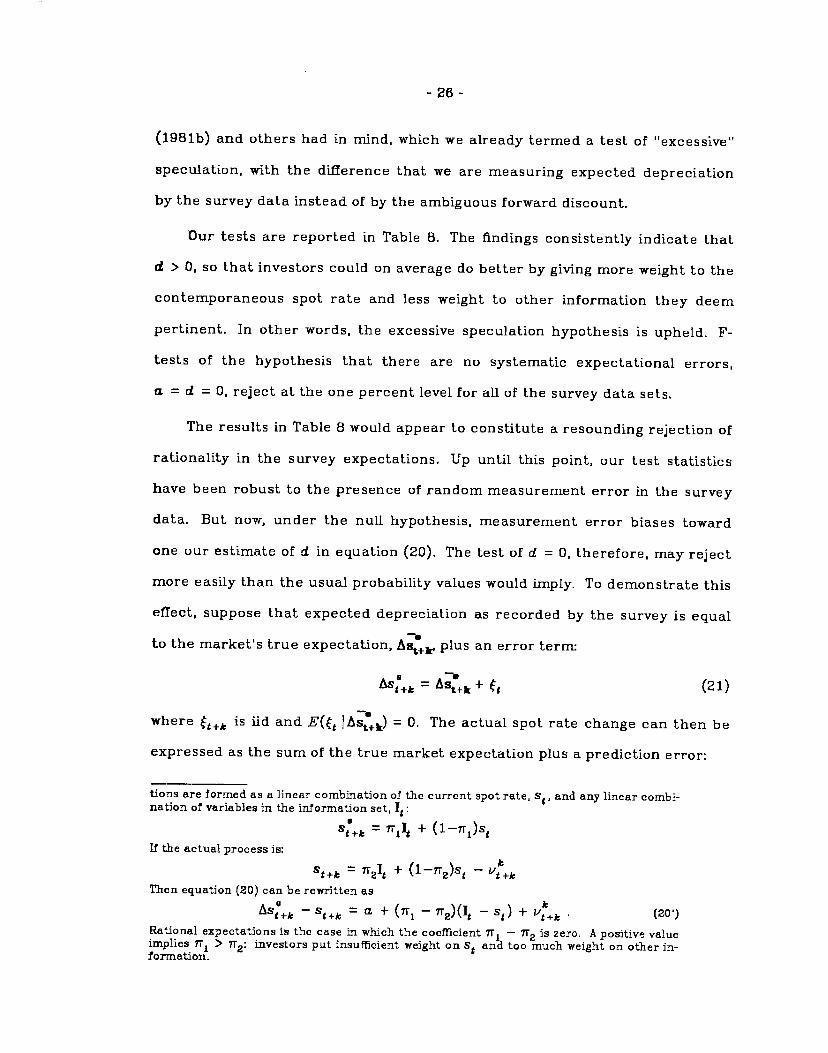
- 26 -

(1961b) and others had in mind, which we already termed a test of "excessive'

speculation, with the dierence that we are measuring expected depreciation

by the survey data instead of by the ambiguous forward discount.

Our tests are reported in Table 8. The findings consistently indicate that

ci > 0, so that investors could on average do better by giving more weight to the

contemporaneous spot rate and less weight to other information they deem

pertinent. In other words, the excessive speculation hypothesis is upheld. F-

tests of the hypothesis that there are no systematic expectational errors,a = ci = 0, reject at the one percent level for all of the survey data sets.

The results in Table 8 would appear to constitute a resounding rejection of

rationality in the survey expectations. Up until this point, our test statistics

have been robust to the presence of random measurement error in the survey

data. But now, under the null hypothesis, measurement error biases toward

one our estimate of d in equation (20). The test of d = 0, therefore, may reject

more easily than the usual probability values would imply. To demonstrate this

efTect, suppose that expected depreciation as recorded by the survey is equal

to the market's true expectation, plus an error term:

= S1÷k + (21)

where is iid and E(E st°k) = 0. The actual spot rate change can then be

expressed as the sum of the true market expectation plus a prediction error:

tions are formed as a linear combination of the current spot rate, S,and any linear coinbi-nation of variables in the information set, l:

= + (i—ii-1)sIf the actual process is:

= 112; + (1—ir2)s — v+kThen equation (20) can be rewritten as

LSg÷ — = a + (ira — 1r2)(It— s) + 't+k (20')

Rational expectations is the case in which the coefficient 7T — 112 is zero, A positive valueimplies 71 > 712: investors put insufficient weight on S and too much weight on other in-formation.

TABLE 8

TESTS OF EXCESSIVE SPECULATION

Regressions of E(s(t+1)]—s(t+1) an EE4s(t+1)]

F test Prob > F

Data Set Dates B t: 8:0 t: B1 R DF OW a:0, 9:0

Economist Data 6181—12185 1.0162 2.48 U 0.04 0.49 509 4.79 0.000

(0.4104)

Econ 3 Month 6/81-12/85 1.6141 3.46 *1* 1.32 0.26 184 2.91 0.010

(0.4664)

Econ 6 Month 6/81-12/85 2.5325 3.75 *1* 2.27 ** 0.41 174 3.54 0.002

(0.6746)

Econ 12 Month 6/81—12/85 —0.3005 —0.57 —2.48 U 0.67 149 6.32 0.000

(0.5241)

NMS 1 Week, I Month 10/84—2/86 1.2561 3.54 Ut 0.72 0.24 414 6.07 0.000

(0.3544)

MMS 1 Week 10/84—2/86 1.1476 3.90 *1* 0.50 0.14 242 1.84 3.97 0.002

(0. 2939)

MMS I Week, S)JR 10/84—2/86 0.7858 7.09 III -1.93 * 0.18 239 12.42 0.000

(0.1109)

NtIS 1 Month 10/84-2/86 1.3068 2.76 Itt 0.65 0.28 171 3.11 0.010

(0. 4741)

NMS 2 Week, 3 Month 1/83-10/84 1.0494 3.32 11* 0.16 0.59 365 7.87 0.000

(0. 3159)

NtIS 2 Week 1/83-10/84 1.0594 3.69 Ut 0.21 0.23 182 1.74 5.40 0.000

(0. 2870)

NtIS 2 Week, SUR 1/B3-10/84 1.0469 5.77 *5* 0.26 0.16 179 9.42 0.000

(0.1913)

NtIS 3 Month 1/83—10/84 1.0465 2.69 *5* 0.12 0.63 182 7.59 0.000

(0.3895)

AMEX Data 1/76—7/85 2.6082 5.09 Itt 3.14 *1* 0.23 86 4.71 0.000

(0.5123)

AMEX 6 Month 1/76—7/85 2.5693 3.49 Itt 2.13 1* 0.37 45 4.22 0.002

(0.7358)

AMEX 12 Month 1/76—7/85 2.6382 4.54 11* 2.82 5*1 0.50 40 4.24 0.002

(0. 5812)

Notes: All regressions except those marked SUR are estimated using 019, with Method of Moments standard errors (in

parentheses). SUR regressions report asymptotic standard errors. Durbin-Watson statistics are reported for data

sets in which the forecast horizon is equal to the sampling interval. I Represents significance at

the 1O level, U and III represent sigrificarice at the 5 and I 1eve1s respectively.

- 27 -

—C kt+k = t+k+ 11+k (22)

Using these facts, the coefficient d in equation (20) converges in probability to:

var(E) —cov(?÷k,_t.I-k)ci = ————————— —

(23)var() + var(Ask)

Measurement error therefore biases our OLS estimates toward one. Indeed, in

the limiting case in which the measurement error accounts for all of the varia-

bility of expected depreciation in the survey -- in other words, no information

at all about the "true" market expectation is contained in the surveys -- the

parameter estimate would be statistically indistinguishable from one. In Table

8, 13 of 15 estimates of ci are greater than one; in five cases the difference is

statistically significant. This result suggests that measurement error is not the

source of our rejection of rational expectations. However, we shall now see that

stronger evidence can be obtained.

5.2. Another Test of Excessive Speculation

One way to get around this added source of noise is to use the projection of

the survey expectations onto investors' information set as the right-hand-side

variable in equation (20). Thus we seek a proxy for the survey expectations.The candidate must be highly correlated with the survey expected depreciation,

and conditionally independent of the measurement error, E(E Jfd) = 0. In

view of the results from section 4, the forward discount seems eminentlyqualified. The usual instrumental variables estimation procedure is not neces-

sary in this case because the null hypothesis is that d 0. Thus we run the OLS

regression:

—Sg+k a1 + + 1.t+k (24)

and perform a test of rationality, a1 = 0.

TABLE 9

TESTS OF RATIONAL EXPECTATIONS

OLS Regressions of EEs(t+1)]—s(t+l} on fd(t)

F test

Data Set Dates B t: B=O R OF a:0, 8=0 Prob > F

Econoiist Data 6/81—12/85 1.4903 1.41 0.48 509 4.75 0.000

(1.0580)

Econ 3 Month 6/81—12/85 2.5127 1.95 0.14 184 1.31 0.256

(1.2918)

Econ 6 Month 6/81-12/85 2.9866 1.87 * 0.28 174 1.46 0.194

(1.5974)

Ecan 12 Month 6/81—12/85 0.5174 0.42 0.67 149 6.01 0.000

(1.2290)

NNS I Month 10/84—2186 15.3945 2.42 *1 0.20 171 2.54 0.030

(6. 3520)

MNS 3 Month 1/83-10/84 6.0725 2.60 It 0.66 182 11.93 0.000

(2.3392)

AMEX Data 1/76-7/85 3.2452 2.78 Itt 0.33 86 2.69 0.005

(1.1675)

AMEX 6 Month 1/76-7/85 3.6346 2.70 1*1 0.26 45 3.30 0.009

(1.3437)

AMEX 12 Month 1/76—7/85 3.1081 2.40 It 0.25 40 1.48 0.210

(1.2954)

Notes: Method of Moments standard errors are in parentheses. I Represents significance at the

10 level, *1 and *1* represent significance at the 57. and 1 levels, respectively.

- 28 -

Equation (24) has additional relevance in the context of our decomposition

of the forward rate unbiasedness regression in section 3: the coefficient, fi1, is

precisely equal to the deviation from unbiasedness due to systematic prediction

errors, fi,.. Thus equation (24) can tell us whether the large positive values of

fi,. found in column (1), Tables 5a and 5b are statistically significant.

Table 9 reports OLS regressions of equation (24). We now see that the pointestimates of fi,. in Tables 5a and 5b are measured with precision. The data con-

tinue to reject statistically the hypothesis of rational expectations,a1 = 0, fi1 = 0. They reject fi1 = 0, in favor of the alternative of excessive specu-

lation. (Because the measurement error has been purged, the levels of

significance are necessarily lower than those of Table 8.) Thus the result that

is significantly greater than zero seems robust across different forecast

horizons and different survey samples. In terms of the decomposition of the

typical forward rate unbiasedness test in Table 5a, we can now reject the

hypothesis that all of the bias is attributable to the survey risk premium. Put

differently, even after allowing for measurement error, it is still not possible to

reject the hypothesis that all the bias consists of repeated expectational errors

made by survey respondents, and that no positive portion of the bias can attri-buted to the survey risk premium.

- 29 -

6. CONCLUSIONS

(1) The survey data indicate that forward rate prediction errors do not give

insight into the nature of the risk premia as commonly thought. In all three

surveys, the errors exhibit unconditional bias of a sign opposite to estimates of

the risk premium from the survey data. The prernia are large in absolute value,

and are statistically different from zero. We can reject the hypothesis that sys-

tematic unconditional mistakes made by the forward rate in predicting the

future spot rate are due entirely to a failure of rational expectations. But at

the other extreme, the hypothesis that the forward rate prediction errors can

be explained by the risk premium alone is also rejected.

(2) Expected depreciation is more variable than both the forward discount and

the risk premium. The first finding corroborates Fama's (1984) conjecture that

expected depreciation and the risk premium are negatively correlated. The

second finding rejects the hypothesis that the variance of expected deprecia-

tion is less than the variance of the risk premium, let alone the more extreme

random-walk hypothesis that the variance of expected depreciation is zero.

(3) Direct tests of perfect substitutability across assets denominated in

different currencies produce mixed results. We find evidence against a time-

varying risk premium, in the respect that changes in expected depreciation are

on average matched, one for one, with changes in the forward discount. In

terms of point (2). changes in the forward discount appear to be unrelated to

changes in risk. The hypothesis of no risk premium fails in our regressions.

however, because the level of expected depreciation is significantly different

from the forward discount by a constant term. In short, while the survey data

do support the existence of a substantial risk premium, they suggest that the

many previous citations of forward discount bias as evidence for the exchange

- 30 -

risk premium may have been misplaced.

(4) While changes in the forward discount reflect changes in expected deprecia-tion, they seem to be, if anything, negatively related to future spot ratechanges. Significantly negative coefficients in regression tests of forward

discount unbiasedness, a common finding in many previous tests, are also found

here. The survey data indicate that this large and significant deviation from

unbiasedness is overwhelmingly due to repeated forecasting mistakes made by

survey respondents. As in the unconditional case in point (1), we are unable to

reject the hypothesis that the conditional deviation from unbiasedness is due

entirely to a failure of rational expectations. We able to reject the compet-

ing hypothesis that the deviation from unbiasedness ispurely a consequence ofthe risk premium. The implication is that, when forming their expectations,investors would do better to put more weight on the contemporaneous spotrate, and less weight on all other variables on which theyrely. This is the same

result that Bilson and many others have found with forward market data; butnow it cannot be attributed to a risk premium.

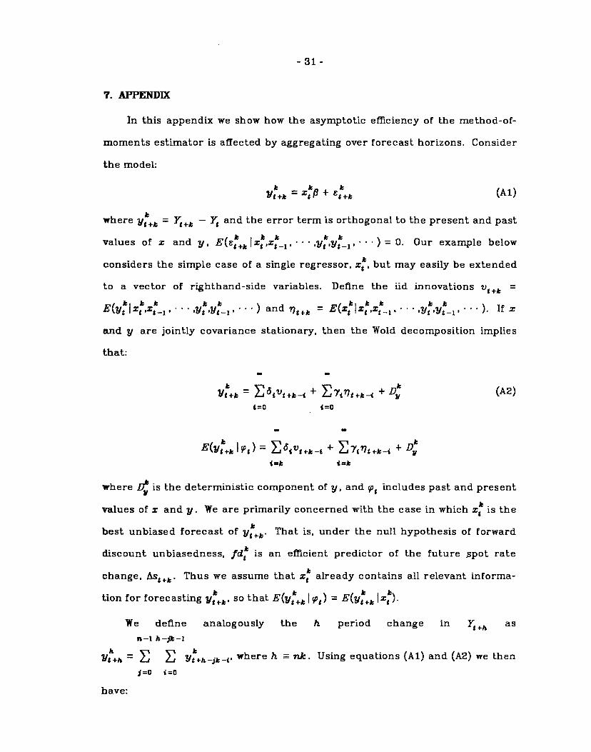
- 31 -

7. APPNDTX

In this appendix we show how the asymptotic efficiency of the method-of-

moments estimator is affected by aggregating over forecast horizons. Consider

the model:

ft ft ft= + (Al)

where = — and the error term is orthogonal to the present and past

values of z and y, E(÷ft ) = 0. Our example below

considers the simple case of a single regressor, x, but may easily be extended

to a vector of righthand-side variables. Define the lid innovations =

ft kk ft ft ft kk ft ftE(y IXg ,x1 , ,y ,y_1 . ) and = E(zg txg x •

. . . ). If 2

and y are jointly covariance stationary, then the Wold. decomposition implies

that:

ft '-' ftVg+ft

= LiôVg+ft_i + 2j7?7gft_. + (A2)

a aft ft

E(vt÷k I) = + + Di

where is the deterministic component of y, and includes past and present

values of x andy. We are primarily concerned with the case in which is the

best unbiased forecast of Yg÷ft That is, under the null hypothesis of forward

discount unbiasedness, is an efficient predictor of the future spot rate

change, S4ft. Thus we assume that z already contains all relevant informa-

tion for forecasting Yg÷ft' so that E(y÷ft E(yft lz).We define analogously the h period change in as

,i-I h-jk-1

= E E YfhJkV where h nk. Using equations (Al) and (A2) we then1=0 i=0

have:

- 32 -

n—i n—i

= E E âVg+h_j + E fh-Jk-i + (AZ')J=Oi=0 J=0%=0

n—i n—i11 h

E(yt+h I9) L1 ôjVt÷h_jk_ + l.j Y;?+h—jk—i +

50%h—jk j=O;h—jk

These facts imply that the Jc and h period prediction errors, and

respectively, are stationary with finite second moments. If we assume that= and = are stationary with finite variance, thenkk . hh ftE(qgqg) = 0 for ,i k, and E(q g÷) = 0 for j h. Thus qg can be expressed

as a k —1 order moving average process:

k—i

ft vi(A3)

i =0

Similarly, from equation (AZ') we have that q may be written as a h —1 order

moving average process:

n—i h-i= E E djvg÷hJftj (A3')

1=0 =0

n-i ft

= E E (—5k — + aft +h (A4)5=0 =0

n -2

where Chjki = E d(fl_m)kj• The covariance generating function for ismJ

denoted by X(z), where

k—i k—i k—i

xa(z) = E x: = E E a5a28 . (A5)5i-kj=0

Using equation (A4), the covariance generating function for can be written

as:

- 33 -

n(n+1) n(n—l)xd() = Xc(z) + XG(z) + + 2X0c1(z) (A5')

2 2

where X'(z) is a complicated generating function of the as's and ci's which we

need not specify here. Finally, the covariance generating function, X'(z) =h—i h—I

2'c-a L1 L1 a5d,+5 can be rewritten as:•=1—k 1=0

{n+l) (n—i)X(z) = X(z) + —— + (A6)2 2

where X2(z) is another generating function of the as's and c1's.

Now consider the asymptotic MoM covariance matrix of 'JT(p — ) from

equation (Al):

& =(x:i-2 Aa() (A7)

7'

k —1 kk -where = T If we add in the longer-term forecast data, our model

is that of equation (11) above, with asymptotic covariance matrix:

=(x. + x)2 (Xd(z) + Xa(Z) + 2X(z)) (A8)

By substitution, we have that & > if and only if:

—1+—— (A9)

2 _____ ____ Xa(z)÷xc(z)+2(XacI(z)+xac2(z))_X:>fl 3f1+ +n33+ - +

X(z) XU(z)

Equation (A9) says that the variance of the longer-term data, X, must increase

at a rate the same as or greater than the relative forecasting interval, n, if we

are to gain by adding longer-term forecasts to data sets of only shorter-term

forecasts. Thus as the forecasting interval increases, we require correspond-

- 34 -

ingly greater variability of the regressors in order to compensate for the

greater variability of the forecast errors.

One might think that the result in equation (A9) is a consequence of

weighting the more imprecise longer-term predictions equally with the predic-tions of shorter-term. Perhaps if we downweighted the longer-term data, we

would always gain in efficiency. It turns out that this is not the case. In the

remaining space, we construct a consistent, optimally weighted estimator and

show that the efficiency of this estimator may still worsen asymptotically by

adding in the longer-term forecasts.

In most circumstances, GLS represents the optimal weighting strategywhen the data have different levels of precision. GLS is, however, inconsistentwhen used on a model with overlapping observations. Thus we consider instead

a weighted least squares estimator which is optimal within a class of consistent

estimators. Consider a transformation of the model in equation (ii), whichstacks the shorter- and longer-term data:

Wy = Wxfl+ Wv1 (AlO)

where W is a diagonal matrix. The MoM estimate of in equation (Alo), , will

be consistent for any arbitrary diagonal matrix W. To see this, note that theMoM estimate of equation (Alo), P may be written as:

Xr'Wx XTI7(, — p) ——(All)

27 —1 271 22 1 2= — zi w1 —

z1v

The final term in equation (All) converges in probability to zero, provided thatthe error term in equation (Alo) is conditionally independent of the contem-

- 35 -

poraneous value of the regressor, E(v x) = 0 (this is just the Gauss-Markov

assumption required for the consistency of OLS in estimating equation (AiD)).

Suppose now that we choose W optimally in order to maximize the gain in

efficiency from adding longer-term forecasts to our shorter-term data. That is:

max

(A12)

where is the MoM asymptotic covariance matrix of

= (A13)

By normalizing the weight on every shorter-term data point to one, it is

straightforward to show that the optimal weight placed on each longer-term

observation is:

ha kadX0X (z)—X0X (z)

= ——(A14)

xxd(z) —XX(z)

Note that will always be positive if the data sets are uncorrelated, i.e. if

X(z) = 0. In other words, appropriately weighted independent information

can always improve efficiency, no matter how imprecise the new information

may be. But, the nature of the correlation between contemporaneous longer-

term and shorter-term predictions implies that the optimal weight given to

longer-term data may be zero. In particular, Wh will be zero if the numerator in

equation (A14) becomes negative. This occurs if n is too large in comparison

with the relative variance of the longer-term forecasts. Using equations (AS').

(AG) and (AlA), it can be shown that a sufficient condition for to be zero is:

(n+i)> ——. (Ai5)

2

Thus, while the standard errors reported in the text indicate that for small

values of n one may obtain improvements in efficiency, this result is not likely

- 36 -

to apply MoM estimation of data with considerably longer forecast horizons,even when the data are downweighted to account for the greater variance ofthe longer-term forecast errors. It is worth stressing in closing that this poten-tial loss in efficiency is a direct consequence of our limited information MoM

estimation strategy. Full information techniques, such as maximum likelihood

estimation, will consistently achieve nonzero gains in asymptotic efficiency withthe addition of longer-term data.

- 37 -

B. REFERENCES

Bilson, John, "The Speculative Efficiency Hypothesis," Journal of Business, July1981. 54, 435-51 (1981a).

"Profitability and Stability in International Currency Markets,"NBER Working Paper, No. 664. April 1981 (1981b).

___________ "Macroeconomic Stability and Flexible Exchange Rates", AmericanEconomic Review, May 1985. 75, 62-57.

Boothe, Paul and David Longworth, "Foreign Exchange Market Efficient Tests:Implications of Recent Empirical Findings," Journal of International Moneyand Finance, 1986.

Cumby, Robert, and Maurice Obstfeld, "Exchange Rate Expectations and Nomi-nal Interest Differentials: A Test of the Fisher Hypothesis," Journal ofFinance, 1981, 36, 697-703.

Dornbusch, Rudiger, "Exchange Rate Risk and the Macroeconomics of ExchangeRate Determination," in R. HawkIns, R. Levich, and C. Wihlborg, eds., TheInternationalization of Financial Markets and National Econorrz.ic Policy,Greenwich, Conn., JAJ Press, 1983.

Fama, Eugene, "Forward and Spot Exchange Rates," Journal of MonetaryEconomics, 1984, 14, 319-338.

Frankel, Jeffrey A., "The Diversifiabiity of Exchange Rate Risk," Journal of Inter-national Economics, 1979, 9, 379-393.

______________ "In Search of the Exchange Risk Premium: A Six-Currency TestAssuming Mean-Variance Optimization," Journal of International Money andFinance, 1982, 1, 255-274.

_______________ "The Implications of Mean-Variance Optimization for Four Ques-tions in International Macroeconomics," Journal of International Moneyand Finance, 1985.

Frankel, Jeffrey A. and Kenneth A. Froot, "Using Survey Data to Test Some Stan-dard Propositions Regarding Exchange Rate Expectations," NBER WorkingPaper, No. 1672. Revised as IBER Working Paper, No. 85-11, University ofCalifornia, Berkeley, May 1986.

___________________________________ "The Dollar as a Speculative Bubble: ATale of Fundamentalists and Chartists," NBER Working Paper, No. 1854,March 1986.

Gregory, Allan W., and Thomas H. McCurdy, "Testing the UnbiasednessHypothesis in the Forward Foreign Exchange Market: A SpecificationAnalysis," Journal of International Money and Finance, 1984, 3, 357-358.

- 38 -

Hansen, Lars Peter, "Large Sample Properties of Generalized Method ofMoments Estimators," Econometrica, 1982, 50, 1029-1054.

Hansen, Lars and Robert Hodrick, "Forward Rates as Optimal Predictors ofFuture Spot Rates: An Econometric Analysis," Journal of Political Economy,October 1980, 88, 829-53.

Hodrick, Robert, and Sanjay Srivastava, "An Investigation of Risk and Return inForward Foreign Exchange," Journal of International Money and Finance,April 1984, 3, 5-30.

________________________________ "The Covariation of Risk Premiums andExpected Future Spot Rates," Journal of International Money and Finance,1986.

Huang. Roger, "Some Alternative Tests of Forward Exchange Rates as Predictorsof Future Spot Rates," Journal of International Money and Finance August1984, 3, 157-67.

Krasker, William. "The 'Peso Problem' in Testing the Efficiency of ForwardExchange Markets," Journal of Monetary Economics, April 1980, 6, 269-76.

Levich, Richard, "On the Efficiency of Markets of Foreign Exchange," in R. Dorn-busch and J. Frenkel, eds., International Economic Policy. Johns HopkinsUniversity Press, Baltimore: 1979, 246-266.

Litterman, R.B. "Bayesian Procedure for Forecasting with Vector Autoregres-sions," M.I.T., 1980.

Longworth, David, "Testing the Efficiency of the Canadian-U.S. Exchange MarketUnder the Assumption of No Risk Premium," Journal of Finance, March1981, 36, 43-49.

McCulloch, J.H., "Operational Aspects of the Siegal Paradox," Quarterly Journalof Economics, February 1975, 89, 170-172.

Mussa, Michael, "Empirical Regularities in the Behavior of Exchange Rates andTheories of the Foreign Exchange Market," Carnegie-Rochester Series onPublic Policy, Autumn 1979, 11, 9-57.

Newey, Whitney and Kenneth West, "A Simple, Positive Definite, Heteroskedastj-city and Autocorrelation Consistent Covariance Matrix," Woodrow WilsonSchool Discussion Paper, No. 92, May 1985.

Tryon, Ralph. "Testing for Rational Expectations in Foreign Exchange Markets,"Federal Reserve Board International Finance Discussion Paper, No. 139,1979.