NBER WORKING PAPER SERIES MARKET … · NBER WORKING PAPER SERIES MARKET STRUCTURE AND INTERNATIONAL TRADE: BUSINESS GROUPS IN EAST ASIA Robert C. Feenstra Tzu-Han Yang Gary G. Hamilton

NBER WORKING PAPER SERIES

MARKET STRUCTURE ANDINTERNATIONAL TRADE:

BUSINESS GROUPS IN EAST ASIA

Robert C. FeenstraTzu-Han Yang

Gary G. Hamilton

Working Paper No. 4536

NATIONALBUREAU OF ECONOMIC RESEARCH1050 Massachusetts Avenue

Cambridge, MA 02138November, 1993

The research on this paper has been supported by the Pacific Rim Business and DevelopmentProgram (PACBAD) at the Institute of Governmental Affairs, University of California, Davis.Financial support from the Ford Foundation is gratefully acknowledged. This paper is part ofNBER's research program in International Trade and Investment. Any opinions expressed arethose of the authors and not those of the National Bureau of Economic Research.

NBER Working Paper #4536November 1993

MARKET STRUCTURE ANDINTERNATIONAL TRADE:

BUSINESS GROUPS IN EAST ASIA

ABSTRACT

In this paper we study the effect of market structure on the trade performance of South

Korea, Taiwan, and Japan. We center our analysis on Korea and Taiwan, countries which

have very different market structures: Korea has many large, vertically-integrated business

groups known as chaebol, whereas business groups in Taiwan are smaller and horizontally-

integrated in the production of intermediate inputs. The exports of these countries to the

United States are compared using indexes of product variety and "product mix", which are

constructed at the 5-digit industry level. It is found that Taiwan tends to export a greater

variety of products to the U.S. than Korea, and this holds across nearly all industries. In

addition, Taiwan exports relatively more high-priced intermediate inputs, whereas Korea

exports relatively more high-priced final goods. We argue that these results confirm the

importance of market structure as a determinant of trade patterns.

Robert C. Feenstra Tzu-Han YangDepartment of Economics Council for Economic Planning andUniversity of California - Davis DevelopmentDavis, CA 95616-8578 Executive Yuan. TAIWAN R.O.C.and NBER

Gary G. HamiltonDepartment of SociologyUniversity of California - DavisDavis, CA 956 16-8578

1. IntroductionSince the early 1 980's, imperfectly competitive market structures have been

incorporated into theories of international trade.1 These new theories were

motivated by empirical observations such as the large amount of intra-inciustry or

two-way trade in similar products between countries, and retied on the development

of tractable models of monopolistic competitior It is now common to incorporate

intra-industry trade, due to monopolistic competition, into the specification of

equations explaining trade flows. However, it can be argued that these estimating

equations depend to a rather limited extent on the market structure. For example,

Helpman (1987) notes that his specification of trade volume equations Consistent

with monopolistic competition also applies when countries are specialized in

different products for any other reason.2 In other words, these empirical methods

that incorporate intra-industry trade do not directly test the importance of market

structure.3

Market structure hasalso been a focus of current research in sociology

dealing with the network structure of modern economies (see the survey by

PowelL, 1990). A network refers to linkages among firms arising from

relationships based upon common ownership, shared production or distribution of a

commodity, or shared fiscal control, such as through a holding company or bank. For

example, a production network represents the firms linked together, from the early

to final stages of production, to produce a finished product; a distribution network

would trace the firms that take the product to the final consumers.

Particular attention has been paid to the differences among network

structures within the rapidly developing countries in East and Southeast Asia, as

well as the differences between these countries and other parts of the world.4 It

has been found that business networks in Japan and South Korea consist of

interlinkages among many sizes of firms, with the larger firms integrating and

coordinating the activities of the smaller firms in the production and distribution

of many major commodities. The largest firms, in turn, are connected through

common ownership. By contrast, production networks in Chinese areas, such as in

Taiwan and Hong Kong. typically consist of close linkages among similarly sized,

mostly small and middle-sized, independently owned firms. These production

networks rely, at an arm's length, on other firms and other networks to supply

inputs and to distribute products.

Although these sociological studies have been reasonably effective at

documenting the differences among networks across countries, they have not

demonstrated that these networks have any direct economic impact, such as on

international trade. In this paper we propose to combine the sociological data on

networks with economic hypotheses about the performance of firms, in order to

demonstrate that market structure indeed has a significant economic impact on

international trade.

We shall focus on one particular type of network - the common ownership of

firms within a business group - and contrast the influence of these groups on the

trade performance of South Korea, Taiwan, and Japan. We will center our analysis

on Korea and Taiwan. countries which have very different market structures. Korea

has many large, vertically-integrated business groups known as chaebol. whereas

business groups in Taiwan are smaller and horizontally-integrated in the production

of intermediate inputs, but do not participate in the production or distribution of

final products. Because the two countries are at roughly similar stages of

development (measured by per-capita GNP), the sharp difference in the market

structures between these two economies are ideal for a comparative study (as also

conducted by Levy, 1991, and Rodrik, 1993). Since the keiretsu are so well-known.

we shall also include Japanese business networks in our analysis.5 Including Japan

allows us. moreover, to contrast the trade performance of a more developed economy

with that of developing economies.

2

In section 2. we describe the business groups in the three countries more

carefully. In section 3. we use this information to construct a stylized model of

business groups and trade performance. The essential features of the model are

that new intermediate inputs can be created to enhance the productivity of

downstream purchasers. The business groups in Korea are treated as vertically

integrated. i.e. they supply some of their own inputs, whereas the firms in Taiwan

purchase all inputs from non-affiliated firms. The model suggests that the

production of final goods in Korea is subject to increasing returns to scale within a

group, so that firms will choose to focus production on a narrow range of products.

but at a potentially high volume. In contrast, firms in the stylized Taiwan economy

will produce a greater range of product varieties.

In section 4 we consider how to empirically test the hypotheses from the

stylized model. The data used are U.S. imports or highly disaggregate products from

Korea, Taiwan and Japan. Using the techniques from Feenstra (1993), indexes of

product variety are constructed at the 5-digit industry level to reflect the range of

products sold from each country. In addition, product mix indexes are constructed

to reflect whether each country tends to export high-priced or low-priced products

within each 5-digit category. We show that both indexes can be theoretically

interpreted as a measure of consumption services provided by the imports.

Our results are presented in section 5. We find that Taiwan tends to export

a greater variety of products to the U.S. than Korea. and this holds across nearly all

industries. In addition, Taiwan has a higher product mix in industries producing

intermediate inputs, whereas Korea has a higher product mix in the final goods

industries. This results are discussed in relation to the theoretical hypotheses, and

in relation to the business group structure of the two economies. We argue that

the results confirm the importance of market structure as a determinant of trade

patterns. A comparison with the Japanese trade pattern is presented, and our

conclusions are summarized in section 6.

3

2. Business Groups in East Asia

2.1 DescriptIons of the Groups

One of the most important features or Korea's industrial organization is the

business groups, or chaebol.6 These groups, consisting of legally-Independent firms.

are affiliated under a common group name and are centrally controlled through

direct family ownership and mutual shareholding among member firms. As shown in

Table I, the 50 largest business groups accounted for 45% of total sales in the

manufacturing sector in 1983. and even more in other sectors. These sales figures

give an inflated estimate of the importance of the chaebol, however, because

transactions of semi-finished goods between firms within a group are included. In

Table 1, the figures in parentheses give the value-added shares accounted for by the

business groups within each sector, and these figures are not affected by the

frequency of intra-group transactions.7 Overall, the value-added of the top 50

business groups accounted for one-fifth of GDP in 1983 (Zeile, 1991).

In the manufacturing, sector, the chaebol spread across many industries. As

shown in Table 2, there were five manufacturing industries in which the chaebol

accounted for more than 50% of the total sales, and eight others in which they

accounted for between 25 and 50%. Many of these are chemical or heavy industries.

This pattern of concentration is a direct result of the government's credit policy.

During the 1970s, the Korean government applied discriminatory interest rates and

controlled both domestic and foreign loans in order to influence industrial

development, it supplied a large amount of credit With low interest rates to

business groups for investment in the heavy and chemical industries, with the result

that these industries and groups grew rapidly.

In general, the chaebol are strongly vertically-integrated. They internalize

many of the production processes (from raw materials to final products) and

distribution processes (domestic and foreign trade) within the business group.8

They form a self-sufficient system known in the Asian business literature as the

4

one-set principled (Gerlach 1992. p. 85). Since the ownership and Policy-making

power are concentrated in the hands of only a few individuals for each group, their

member firms coordinate and cooperate quite well. Transactions with non-

affiliated firms are limited to those inputs that are not available internally.

In Taiwan, business groups are much less dominant in the final export sector.9

The total sales of the 96 largest Taiwanese business groups accounts for only 19%

of sales in the manufacturing sector (see Table 1). As shown in Table 2. they are

influential in a smaller number of manufacturing industries, principally those

producing intermediate goods.1° There is only one industry - textiles - in which the

group share of total sales is over 50%. and another three industries - chemical

materials, non-metallic mineral products, and food products - in which they have a

share between 25 and 50%.

The shares shown in parentheses in Table 2 include the sales of both business

groups and enterprises owned by the state government. The state-owned enterprises

are also concentrated in intermediate goods. Two out of the five industries with

significant government shares - basic metal and petroleum - are obvious upstream

industries. In the food industry, state-controlled enterprises mainly produce sugar.

salt, and animal feeds - all raw materials. In transportation industries, the state

is involved in shipbuilding and highway construction. Adding up the shares of

Taiwanese business groups and state-owned enterprises in the overall economy, their

dominance in intermediate goods industries is quite apparent, with the exception of

fabricated metal, a category that includes both intermediate and final goods.

The smaller size of Taiwanese business groups and their nearly exclusive

focus on intermediate inputs are two of the major distinctions between the

Taiwanese and Korean business groups. Although both economies are heavily export

oriented (Taiwan even more so than Korea). the largest business groups in each

economy occupy very different structural locations: The Korean chaebol dominate in

the export sector, and the biggest business groups in Taiwan produce intermediate

5

.

6

goods that are sold domestically. These domestic sales are primarily to small and

medium size lrms that have only an Thrms length relationship with the producers

of intermediate inputs. Unlike the case in Korea, in Taiwan small and medium sized

firms produce and export on their own without direct assistance from the state or

from big businesses. Closer inspection of the holding of the large business groups

in Taiwan shows that they typically concentrate their investments in a single core

upstream business, and then diversify additional investments in unrelated areas.1 1

Based on self-reported information, over 40% of Taiwan's business groups reported

that none of their member firms were linked by ongoing business transactions. An

additional 33% reported five or fewer routine transaction linkages among member

firms.12

In Japan. the independent firms in intermarket business groups mutually own

each other shares. For any one firm, the controlling interest is held only by the

group as a whole (Orru. Hamilton. and Suzuki 1990; Gerlach 1992). Typically,

individual ownership, whether through stock or through private holdings, accounts

for very little of the total ownership of Japanese business groups. Most firms are

publicly listed on one of Japan's large stock exchanges, but only a small percentage

of the total shares are actually available for purchase. Most equity in business

group firms is held by other firms in the same business group.

Structurally speaking, there are two types of business groups in Japan: one a

horizontally and the second a vertically arranged network among firms (Orru,

Hamilton, and Suzuki 1989; Gerlach 1992). The first type, known as intermarket

groups, or intermarket keiretsV have ownership and loan relationships that extend

across unrelated industries. The major firms in these groups. along with a set of

relatively autonomous, very large firms (e.g. Toyota), organize a second type of

ownership network, called keiretsu or vertical keiretsu. These networks

illustrate the one set principle. They consist of interlinkages among many small.

medium, and large independent firms so that inter-firm networks overlaps directly

with production sequences. The activities of these production networks are

coordinated by the large firms in the network. The data in Tables 1 and 2 includes

the sales of the six major intermarket groups along with ten other vertical

keiretsu.1 In comparison with Korea, the Japanese business groups are more

specialized across industries, and account for substantial shares of sales rn

intermediate industries, chemicals, machinery, electronics and transportation

equipment.

2.2 ExplanatIons for the Groups

From this brief description, it is apparent that the business groups across the

East sian countries differ quite substantially. What causes the differences in

market structures among the countries? One can distinguish two principal

categories of explanation: transaction costs, drawing especially on the difference

in entrepreneurial talent and ties within the countries; and government support

provided to the industries through various policy instruments.

The transactions cost approach seeks to explain the market structure in terms

of the efficiency of making transactions in the market versus the firm. The work

of Williamson (1975, 1985) and others has formalized the nature of these costs -

including ex-ante and ex-post negotiation costs - and how they might differ across

industries. It has also been recognized that transactions costs can differ

substantially across countries, a point that Williamson (1985. p. 9) attributes to

Arrow: Arrow insisted that the problem of economic organization be located in a

larger context in which the integrity of trading parties is expressly considered

(1974). The efficacy of alternative modes of contracting will thus vary among

cultures because of differences in trust (Arrow, 1969. p. 62). Levy (1991)

provides some evidence at this point for the Korea-Taiwan comparison.

Er-ante contracting costs, such as the costs of collecting information and

negotiating. should depend on the education level and the number of people involved

in commercial activities. In education. the percentage of people in Taiwan having

7

more than twelve or more years of education was almost triple that in Korea in

both 1960 and 1970. The absolute number of this educated group was also higher ir'i

Taiwan than in Korea. even though the Korean population was more than double that

of Taiwan. Furthermore. Taiwan has had a greater percentage of the total

population engaged in commercial activity since before the turn of the century.14 In

addition, those engaged in independently run businesses in Taiwan constitute a higher

percentage of the total number of people engaged in business. By contrast, in Korea.

the percentage of employees in the total labor force, as opposed independent

entrepreneurs, is much higher. From a transaction cost perspective, the higher

density of those making independent commercial decisions in Taiwan facilitates the

rapid dissemination of information and encourages entrepreneurship in general.

In the stage of ex-post contracting, the transaction costs arise from the

exercise of opportunistic behavior. To compare these costs across countries, we

adopt Granovetter's (1985) emphasis of the role of social relations in generating

trust and discouraging malfeasance (p. 490). In a society with dense interpersonal

networks and frequent personal interaction, having a reputation for honesty and

reliability becomes an important business asset. In field interviews with

Taiwanese firms, many researchers (Kao, 1991; Numazaki .1991; Shieh, 1 992;

Hamilton, 1993) have found interpersonal trust to be the characteristic most

emphasized in developing business relations. The Chinese words xin (trust-

worthiness), guanxi (reciprocal personal relationships), and renching (human

emotions) denotes the set of personal traits that informants say are evoked to

create and assess reliable business associates.15 The guanxi relationships are

personal networks among peers, especially drawn from extended family, friends,

classmates, and those from the same towns, which form the basis of many business

relations. The networks generated through personal relationships are always more

important for conducting business than are legal contracts (Kao, 1991; Numazaki,

1991). In contrast, in Korea the social relations are more hierarchical in nature

B

(Biggart. 1 ggO), with family, friends or persons from the same region being hired

as subordinates within a business group. An implication of this is that in Korea (or

Japan) it would be unacceptable for an individual to leave one firm and start a

competing firm, whereas this is commonplace in Taiwan, where workers will leave

an enterprise to develop related products.

Thus, the differences in the type of social relation networks found in Taiwan

and Korea appear to mirror the differences in the business group structures. We

would be reluctant to conclude that one factor causes the other, however, and both

features may reflect other underlying differences in the countries. For example.

institutional differences between the countries, such as those governing kinship.

inheritance, and property rights, establish parameters to social relationships that

in turn shape the business strategies people use)6 Among the Chinese, for

instance, the presence of a patrilineal kinship system with partible inheritance

(i.e., all Sons divide the father's estates equally) means that it is difficult for a

family's holding to remainunder central control for more than a few generations

(Wong Siu-Lun. 1985). In contrast, the inheritance pattern in Korea gives a

dominant share to the eldest son, who often retains control over the entire family

holdings.

The transaction cost interpretation is directly related, and is complementary,

to the political economy explanation for the differences in market structure among

East Isian countries: market structure results from state intervention. The very

active government support given the chaebol in the 1970s, through credit policies

and other forms of industrial promotion, helps considerably to explain the market

structure of the Korean economy (Amsden, 1989: Koo. 1984). State support for

business groups has been demonstrated for many other countries, including Japan

(Hadley, 1970; Johnson. 1982) and also Taiwan (Pang, 1992; Numazaki. 1986; Gold.

1987). This link between political and business powers is unquestionably an

important factor in the development of the business groups.

9

3. Model of Business GroupsTo develop the implications of the business groups for economic performance,

we return to a feature of the Korean chaebol: whenever possible, inputs are

obtained from firms within the group. Profit maximization for the group as a

whole implies that these inputs will be supplied at marginal cost to other firms

within the group. Therefore, the vertical-integration leads to an efficiency gain

within the group, resulting in internal economies of scale: as output increases,

more inputs can be produced within the group and sold at marginal cost, leading to

reductions in the cost of producing final goods. Intuitively, we could expect these

internal economies of scale to results in longer production runs over a more narrow

range of output varieties. For this reason, we might expect an economy such as

Korea. with the vertically-integrated groups, to produce less Output varieties than a

non-integrated economy, such as Taiwan. In the section. we will theoretically

confirm this hypothesis in a model of monopolistic competition.

We will suppose that both final goods and intermediates inputs are produced

in many varieties. While the final goods are traded, we will treat the

intermediate inputs as r?ontraded internationally, as with producer services, for

example. Helpman and Krugman (1985. pp. 220-222) have used such nontraded

intermediate inputs to introduce the idea of industrial complexes, in which the

production of inputs and the final goods using them must occur in the same country,

and we will encompass these activities within a business group. For simplicity, we

do not allow for other intermediate inputs that are traded across borders.

Labor is the only primary factor, and is chosen as the numeraire, with one

unit of labor producing one unit of an intermediate input. Production of any variety

of the final good uses both labor and a CES aggregate of the intermediate inputs.

Then the cost of producing one unit of output can be written as +1cC')), where c()

denotes the CES unit-cost function:

10

1-0 11(1-0)c(•) fp(z) dz . (1)

and p(z) is the price of an intermediate input of type Z; 0>1 is the elasticity of

substitution; and (O,MJ is the range or intermediate inputs available to a firm (as

will be specified more fully below). We also adopt a CES utility function to obtatn

demand for the differentiated outputs. with the elasticity of substitution q>1.

It is useful to first solve for the equilibrium product diversity in the

absence of any vertical-Integration: we use the subscript a for this case. We

make the standard assumption that each firm produces only a single variety of th

output or input, and is therefore infinitesimally small compared to the total range

of varieties. It follows that the elasticity of demand for the input varieties is 0,

and for the output varieties is ii. Setting marginal revenue equal to marginal cost.

the price of the intermediate inputs is pa=0/(0-l). Substituting this into (1) we

obtain the unit-costs ca('), and then the price of the output is q8 =

Thus, the profits earned by each of these firms are:

Ttxa (pal)Xakx = (xa/0)-kx, (2a)

(qa — +(ca()1}ya -ku {+(Ca()]/(TI -1 ))ya — k (2b)

where Xa and Ya are the equilibrium quantities sold by the input and output-

producing firms, and kx and k are their respective fixed costs. Under free entry,

the profits in (2) will be zero, and we will denote the equilibrium range of input

and output varieties by Ma and Na. respectively.

In order to determine the range of product varieties, we could use the full-

employment condition in the economy. As a short-cut, however, we can instead

appeal to the equality of GNP measured as the payment to factors or the value of

final output (where we assume the trade is balanced in the final goods sector).

This equality is stated as:

11

L N3qaya Naya4ECa()1T/(T1). (3)

Making use of (3) and (2b) with Tty:O. we immediately solve for the equilibrium

range of output varieties:

Na LJk (4)

Our next task is to determine how vertical-integration will influence the number of

output varieties.

A business group (denoted with the subscript b') will maximize profits over

the ranges of outputs and inputs produced, which implies marginal-cost pricing of

the inputs sold internally. This pricing scheme will have an impact on the unit-

costs +(c(.)J only if the group produces a positive range (measure) of inputs Mb>O.

as we shall assume is the case. These inputs may or may not be sold to other

firms, as we shall discuss below. We will argue below that each group will find it

optimal to produce a positive range of Outputs Nb>O. because the economies of scale

from producing inputs inte,nally also creates economies of scope. The number of

business groups is denoted by G. which will be determined by a zero-profit condition

for the groups. We will also allow for the production of inputs and outputs by non-

integrated firms.

The profits of a business group producing Mb inputs and Nb outputs are:

Ttb NIq - +(cb(.)1}yb -Nbky

• Abxb(pb — 1) - Mbkx. (6)

where b1Mb denotes the range of inputs that the group sells to outside firms, at

the price Pb and quantity Xb. The reason that the group might sell less than the full

range of inputs is that each input leads to a reduction in costs cb(') for another

business group, which will be competing with the selling group in the output

market.

To see how the sale of inputs will affect costs, notice that the CES unit-

costs for a group can be written as:

12

I 1-o 1-0111(1-0)Cb() = [Ma() 4Mb (G 1 )%Pb j . (1 ')

where Ma denote the range of inputs sold by non-integrated firms at the price

01(0-i): Mb is the range of inputs produced by the business group and supplied to

itself at marginal cost; and (G-1)b are the inputs supplied from all other groups

at the price Pb. An increase in the range of inputs Ab supplied from one business

group to another will lower unit-costs in (1'). and therefore increase the

competition in the output market. It is quite possible that groups will choose to

not sell any inputs to each other, or sell only a portion of the inputs that they

produce, depending on whether the profits from selling exceed the losses induced by

the competition in differentiated outputs. While we have worked through some

examples to determine that these various outcomes are possible, our principal

results will not depend on whether business groups sell to each other or not.

Profits of the non-integrated firms producing inputs and outputs can be

written as in (2). where we continue to use the subscript a to denote non-

integrated firms. The variables Ma. xa. Na. and Ya are still interpreted as the

varieties and outputs produced by the non-integrated firms, though of course, their

values will change when there are also business groups in the economy. We must

have ltxa 10 and ltUalO in equilibrium, and several additional results can be obtained

on the sign pattern of profits.

Consider a business group that sells its full range of inputs Mb to other

groups or non-integrated firms. Since this decision may not be optimal, we denote

its profits by ib11tb, where tt,.:O from free entry of business groups. The group

selling all of its inputs must have higher profits than a combination of Mb non-

integrated firms selling inputs, and Nb non-integrated firms selling outputs. so that

Ttb > NbTtya • MbTtxa. This result follows from the efficiency gain within a group

from pricing inputs sold internally at marginal cost, which results in a rise in

profits over the non-integrated firms. However, since b10, it follows that at

13

least one of Txa or Tt must be strictly negative: in addition to the business

groups in the economy. there can be non-integrated firms producing either inputs or

outputs, but not both.

A second result is obtained by comparing MbTtxaIO with the expression

(Rbxb(pb - 1) • Mbkx]. which is a component of grp profits n (6). The term

(Xb(pb 1)kx) is the profits of the business group from selling one input variety to

all outside firms, not including sales to itselr (where profits are zero). Because

the internal sales are not included in the quantity xb. it can be argued that these

profits must be strictly less than ltxa. earned by a non-integrated firm from sales

to all groups and other output-producing firms.1 7 Then using b1Mb. it follows

that Ebxb(pb - 1) Mbkx] <MbTtx.O, so the component of group profits in (6) that

reflect the profits earned from selling inputs must be strictly negative. With

Ttb 0 from free entry, it follows immediately that the profits earned from sale of

outputs, or EN{q — 4cb.)])yb - Nbk), must be strictly positive.

This latter result s a critical feature of the equilibrium. The positive

profits earned from sale of outputs reflect an internal economies of scale from

production of intermediate inputs, thereby lowering costs, but leads to economies of

scope in producing a greater variety of outputs. That is. each additional output

variety that is produced will generate positive profits for the group. ceteris

paribus. As groups become large, however, the expansion of output varieties will

draw demand away from those varieties already produced, and this will serve to

determine the optimal size of a group.

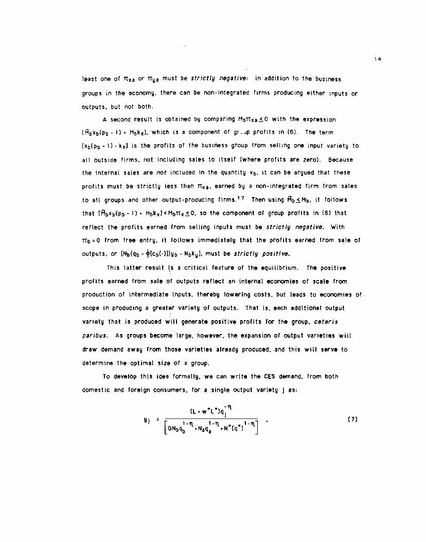
To develop this idea formally, we can write the CES demand, from both

domestic and foreign consumers, for a single output variety j as:

* -rt(L'w L )q.

Yj

[GNbq.Naq.Ncq']

14

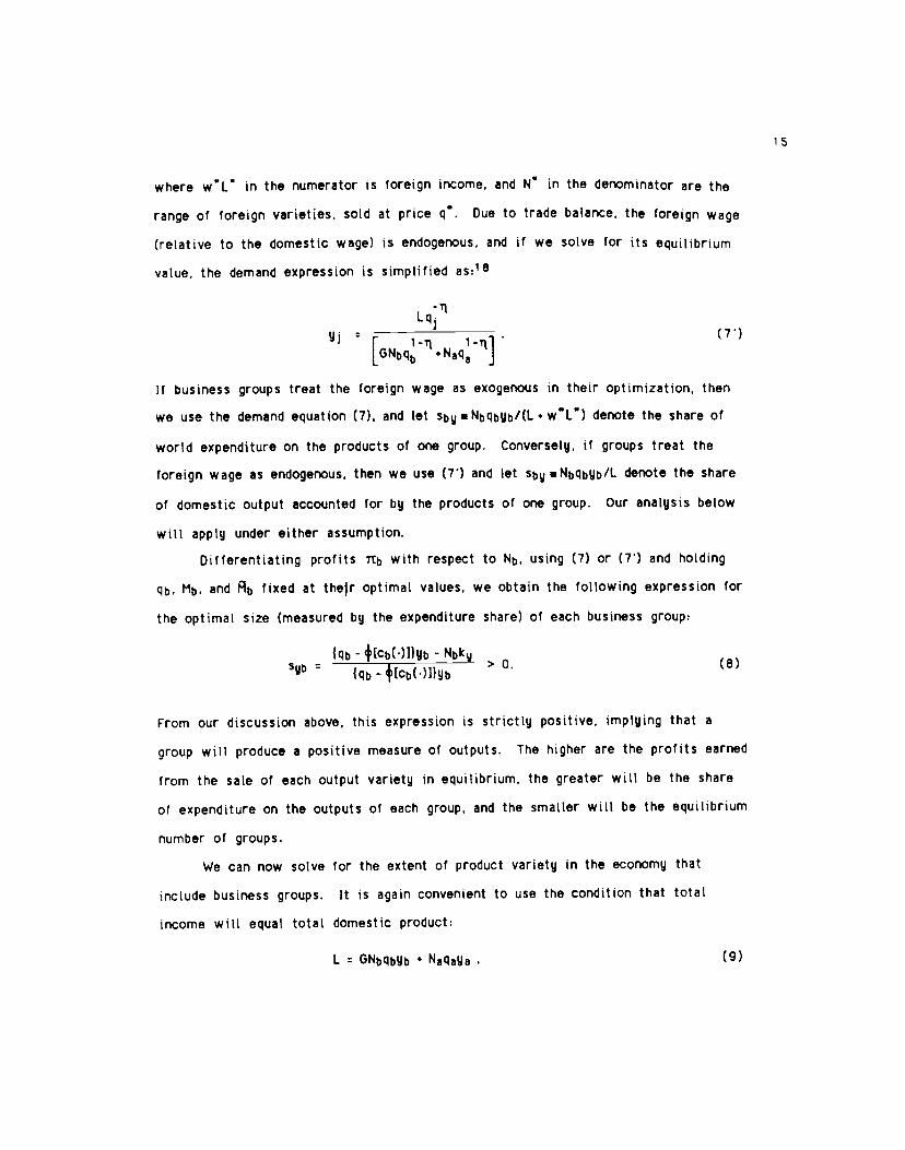
where WL in the numerator is foreign income, and NN in the denominator are the

range of foreign varieties, sold at price q. Due to trade balance, the foreign wage

(relative to the domestic wage) is endogenous. and it' we solve for its equilibrium

value, the demand expression is simplified as:1 8

Lqr i-1[GNbq •Naq j

If business groups treat the foreign wage as exogenous in their optimization, then

we use the demand equation (7). and let sbNNbqbyb/(L+w0L) denote the share of

world expenditure on the products of one group. Conversely, if groups treat the

foreign wage as endogenous. then we use (7') and let sby.Nbqbyb/L denote the share

of domestic output accounted for by the products of one group. Our analysis below

will apply under either assumption.

Differentiating profits Ttb with respect to Nb. using (7) or (7') and holding

qb, M, and Ab fixed at their optimal values, we obtain the following expression for

the optimal size (measured by the expenditure share) of each business group:

{qi - +b(')1Yb NbkySyb

{qb-+Ecb(.)]}yb

> 0. (8)

From our discussion above, this expression is strictly positive, implying that a

group will produce a positive measure of outputs. The higher are the profits earned

from the sale of each output variety in equilibrium, the greater will be the share

of expenditure on the outputs of each group, and the smaller will be the equilibrium

number of groups.

We can now solve for the extent of product variety in the economy that

include business groups. It is again convenient to use the condition that total

income will equal total domestic product:

L GNqbyb • Nqya . (9)

15

where GNb are the total output varieties produced by business groups, and Na are the

varieties produced by non-integrated firms, if they occur. The latter will price at

qa : +afl1(Tl). and from ltya :0 it follows that aYa : r1k. In contrast, the

business groups will charge prices higher than +bnt,'(l_1), since they produce

multiple output varieties. The optimal price for the groups is q +bb/(yb- 1 ),

where t.T4Syb(1_.q) is the elasticity of demand for the entire range of outputs

produced. Substituting these prices into (5). we obtain +byb = ky(eyb-1 )/(1 Syb) =

(i-l)k. Then using the positive profits from the sale of outputs by the group, we

find that bYb +bYb . : rtky. Using this in (10). it follows immediately that,

GNb • Na < L/r1k. (10)

Thus, by comparing this result with (4), we see that the economy with

vertically-integrated business groups will produce a smaller variety of outputs than

the non-integrated economy. The explanation for this result is that the efficiency

resulting from integration is reflected in positive profits on the sale of outputs

(With zero profits overall). These positive profits can be obtained only if the

business groups produce higher output quantity, or longer production runs, than would

a non-integrated firm with the same costs. From the resource constraint for the

economy, these higher output quantities mean that fewer product varieties are

produced in equilibrium.

This hypothesis will be tested empirically in the remainder of the paper. In

addition, we will consider the product mix of each country over high-priced and

low-priced import varieties, which is often used as a proxy for product quality.

Rodrik (1993) argues that reputational considerations for the large Korean chaebol

should lead them to produce at higher qualities than the smaller Taiwanese firms.

This hypothesis is consistent with our model, where the business groups produce

multiple output varieties, and should therefore be more concerned about their

reputation, and we also test for differences in product mix.

4. Empirical Model

4.1 Product Variety and Mix Indexes

In this section. we develop indexes of product variety and product mix for

U.S. imports from South Korea, Taiwan and Japan. For each industry, treat the U.S.

imports from each of these countries as differentiated across i1 N varieties,

where each country j1 J may supply only a subset l.{l N} of these varieties.

Let yj:(g1j.y2j UNJ) denote the vector of import quantities from country j. where

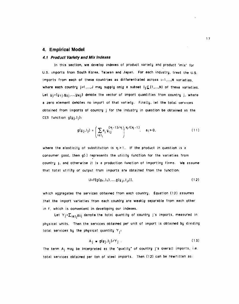
a zero element denotes no import of that variety. Finally, let the total services

obtained from imports of country j for the industry in question be obtained as the

CES function g(yj.Ij):

(-1)/ I'I/(ll-l)g(y.l) a1 y,1

, a1 >0, (11)

icli )

where the elasticity of substitution is Ti >1. If the product in question is a

consumer good, then g() represents the utility function for the varieties from

country j. and otherwise it is a production function of importing firms. We assume

that total utility or output from imports are obtained from the function:

U:F[g(y1 ,li ) g(yj.lj)J. (12)

which aggregates the services obtained from each country. Equation (12) assumes

that the import varieties from each country are weakly separable from each other

in F. which is convenient in developing our indexes.

Let Yj:>1.yij denote the total quantity of country js imports, measured in

physical units. Then the services obtained per unit of import is obtained by dividing

total services by the physical quantity Yj:

• g(y,l)/Y . (13)

The term A3 may be interpreted as the quality of country js overall imports. i.e.

total services obtained per ton of steel imports. Then (12) can be rewritten as:

17

U:F(A1Y1 (1 2)

WhIle the quality variable cannot be measured directly. since it depends on

the unknown level of service g(y.lj). an empirical measure can be obtained by

considering the ratio of relative qualities A1/Ak. Letting qj > 0 denote the price

vector from country j. this ratio can be measured by:1 9

- i'2i (c(qj.Ij)— /1 . (14)

Ak Ek/Yk c(qk.lk))

where E1 denotes total expenditure on imports from country j. and c(q1,l) is the

unit-cost function dual to (11):

( 1-1\1/(1-T1)c(q,l) b1 q1 . b1 = a1 . (15)

tiel1 )

Expression (14) is the ratio of unit-values of imports from country j and k,

divided by the ratio of unit-costs from the two countries. While the unit-values

are directy obtained from import data, the unit-costs are not observed. However,

their ratio can be measured by an exact price index. In particular, suppose that

and y are the cost-minimizing quantities with prices qj and q, respectively, and

that the set of common goods l.(ItCi It-i) imported from both countries is not

empty. Then from Feenstra (1993), the raflo of unit-costs can be measured as:

c(qj.lj)/c(qk.lk) P(qj.qk.yj,yk.l) (Xj/Xk)1 /(i-1)

(1 6)

where:

(a) P(q1 .qk .Yj .yk.I) is the price index of Sato (1976) and Vartia (1976). constructed

over the common goods 1:20

(b) X , qijyij /, qijy with the same formula applying for Xk.itI iI

18

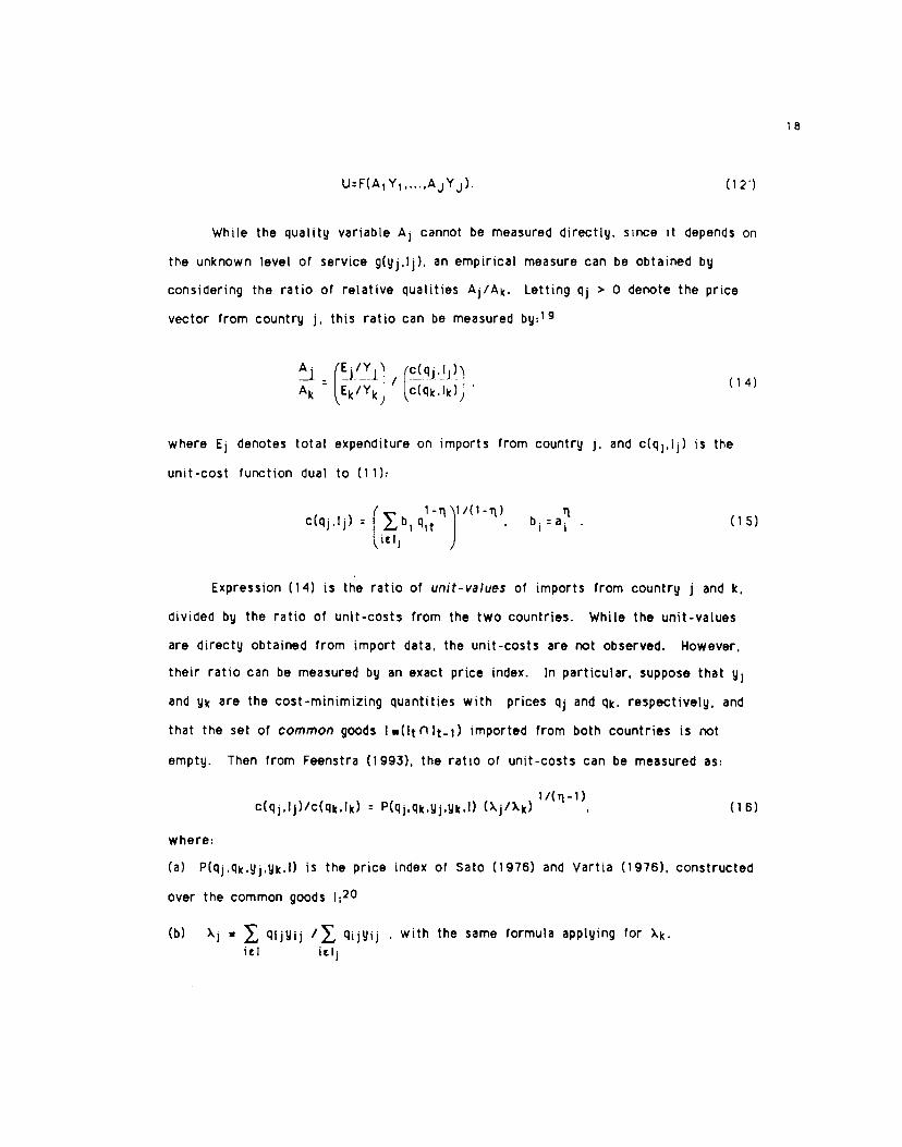
The result in (16) states that the ratio of unit cost of service equals the

price index of the common goods times the additional term (Xj/Xk)1'(h1. To

interpret this term, note that X is the proportion of the expenditure on the

common goods iti relative to the entire set of goods iel. Alternatively, X

measures one minus the expenditure share of the goods outside the set I. if country

has a larger share of revenue from selling the products other than the common

goods, so that X> X. it tends to lower the unit-cost ratio by an amount depending

on the power 1/(q-1). The higher is the substitution elasticity ii. the lower s the

impact of varieties supplied by only one country on its unit-costs.

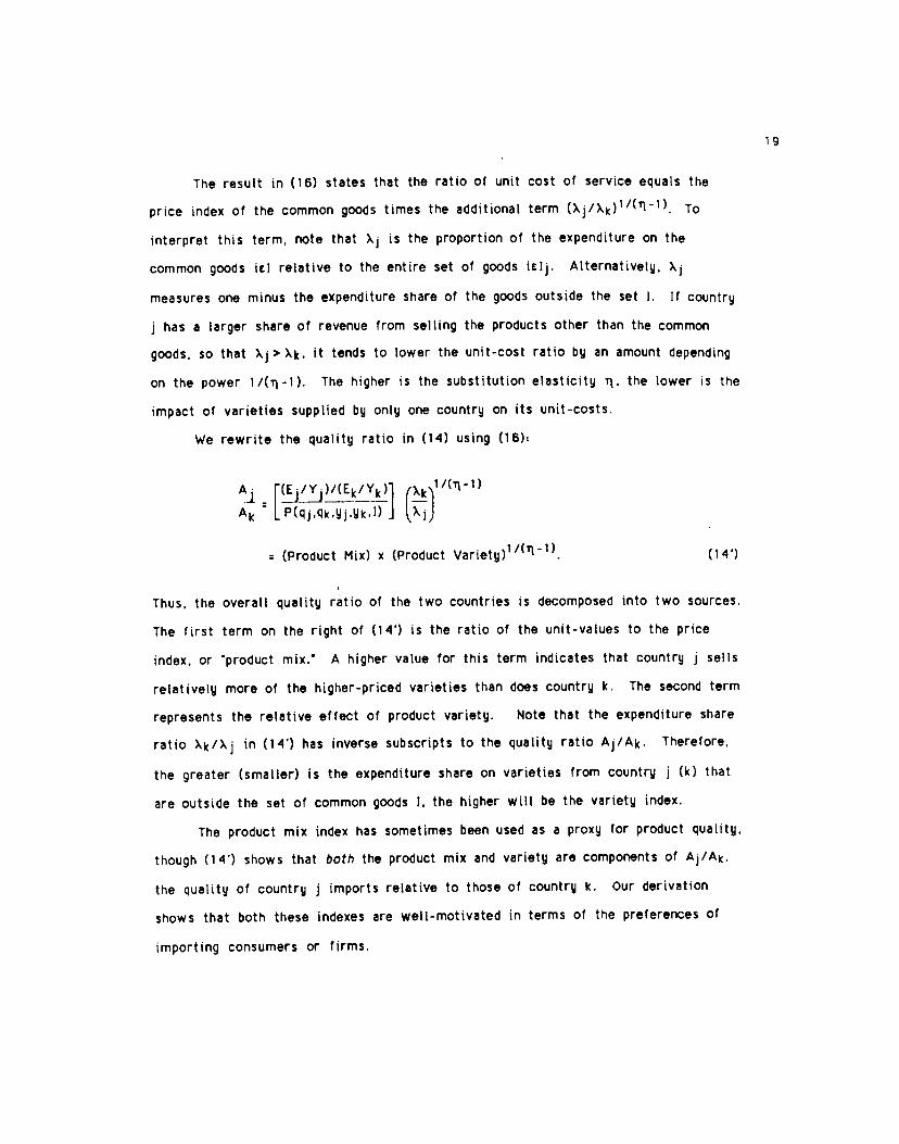
We rewrite the quality ratio in (14) using (16):

A - 1ii !±11 (!11)Ak - [P(q1,qk,y1,yk,I) j X)

(Product Mix) x (Product Variety)1_l). (14')

Thus, the overall quality ratio of the two countries is decomposed into two sources.

The first term on the right of (14') is the ratio of the unit-values to the price

index, or product mix. A higher value for this term indicates that country j sells

relatively more of the higher-priced varieties than does country k. The second term

represents the relative effect or product variety. Note that the expenditure share

ratio Xk/Xj in (14') has inverse subscripts to the quality ratio Aj/Ak. Therefore.

the greater (smaller) is the expenditure share on varieties from country j (k) that

are outside the set of common goods 1. the higher will be the variety index.

The product mix index has sometimes been used as a proxy for product quality,

though (14') shows that both the product mix and variety are components of AJ/Ak,

the quality of country j imports relative to those of country k. Our derivation

shows that both these indexes are well-motivated in terms of the preferences of

importing consumers or firms.

19

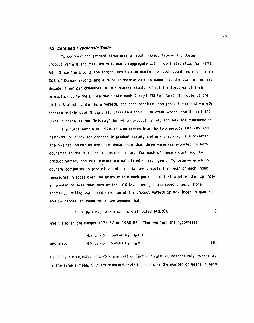
4.2 Data and Hypothesis Tests

To contrast the product structures of south Korea, Taiwan and Japan in

product variety and mix, we will use disaggregate U.S. import statistics for i 978-

88. Since the U.S. is the largest destination market for both countries (more than

30% of Korean exports and 40% of Taiwanese exports came into the U.S. in the last

decade) their performances in this market should reflect the features of their

production quite welt. We shalt take each 7-digit TSUSA (Tariff Schedule of the

United States) number as a variety, and then construct the product mix and variety

indexes within each 5-digit SIC classification.21 In other words, the 5-digit SIC

level is taken as the industry for which product variety and mix are measured.22

The total sample of 1978-68 was broken into the two periods 1978-82 and

1983-88, to check for changes in product variety and mix that may have occurred.

The 5-digit industries used are those more than three varieties exported by both

countries in the full first or second period. For each of these industries, the

product variety and mix indexes are calculated in each year. To determine which

country dominates in product variety or mix, we compute the mean of each index

(measured in togs) over the years within each period, and test whether the log index

is greater or less than zero at the 10% level, using a one-sided t-test. More

formally, letting Znt denote the log of the product variety or mix index in year t.

and p denote its mean value, we assume that:

Znt Pn • tnt. where nt is distributed N(0,), (17)

and t lies in the ranges 1978-82 or 1983-88. Then we test the hypotheses:

H0: p.O versus H1: ji>O

and also, H6: jln>O versus Hj: jin<O . (18)

H0 or Ha are rejected if /S>t0g(t-1) or in/S < -tg(r-1), respectively, where T1

is the sample mean. S is its standard deviation and is the number of years in each

20

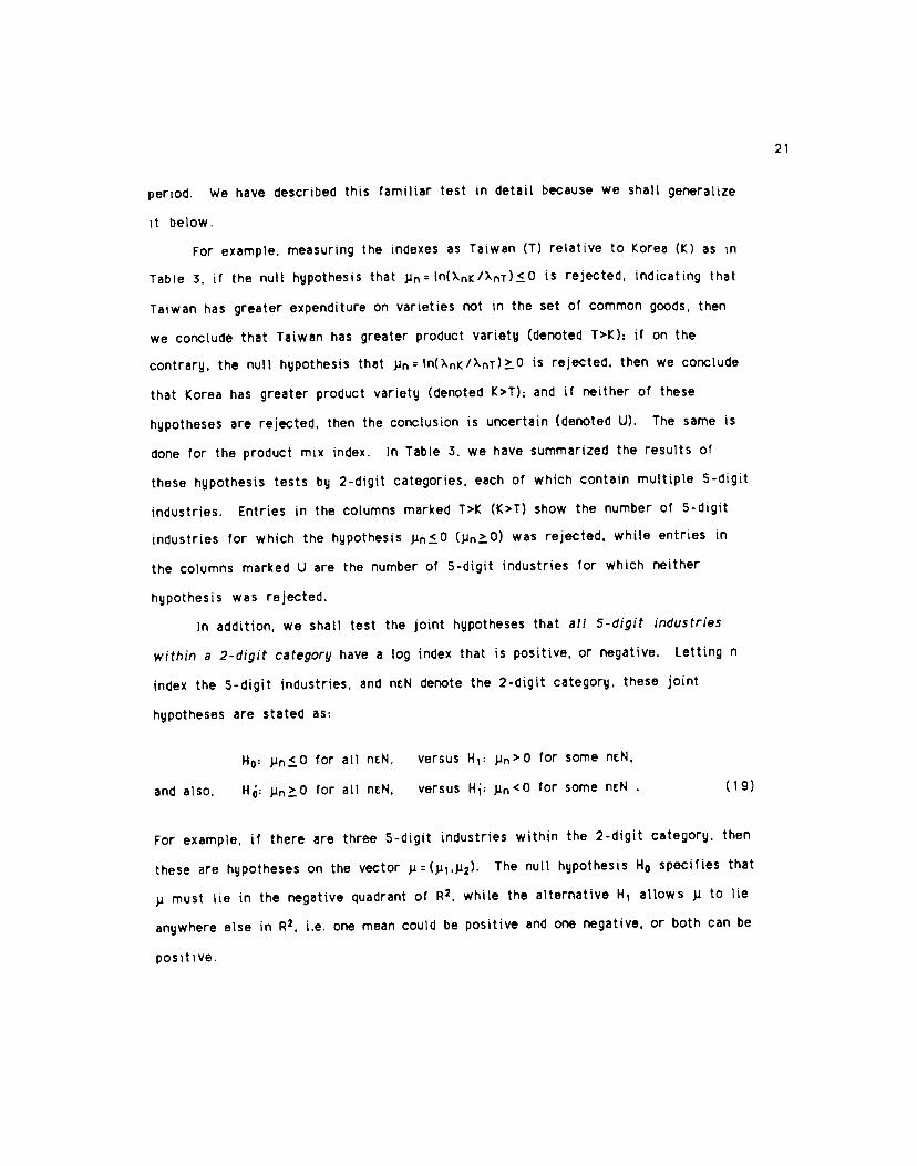
period. We have descnbed this familiar test in detail because we shall generalize

it below.

For example. measuring the indexes as Taiwan (1) relative to Korea (K) as n

Table 3. if the null hypothesis that Mn: ln(XnK/XnT)IO is rejected, indicating that

Taiwan has greater expenditure on varieties not in the set of common goods, then

we conclude that Taiwan has greater product variety (denoted T>K); ii on the

contrary. the null hypothesis that pn: ln(Xn/Xni)O is rejected, then we conclude

that Korea has greater product variety (denoted K>T); and if neither of these

hypotheses are rejected, then the conclusion is uncertain (denoted U). The same is

done for the product mix index. In Table 3, we have summarized the results of

these hypothesis tests by 2-digit categories, each of which contain multiple 5-digit

industries. Entries in the columns marked T>K (K>T) show the number of 5-digit

industries for which the hypothesis j'nIO (p�O) was rejected, while entries in

the columns marked U are the number of 5-digit industries for which neither

hypothesis was rejected.

In addition, we shall test the joint hypotheses that all 5-digit industries

within a 2-digit category have a log index that is positive, or negative. Letting n

index the 5-digit industries, and nN denote the 2-digit category. these joint

hypotheses are stated as:

H0: j1<O for all nN, versus H1: Mn>O for some rieN,

and also, H: Mn0 for all neN, versus Hj: Pn<O for some nN . (19)

For example. if there are three 5-digit industries within the 2-digit category, then

these are hypotheses on the vector y:(p1.j.12). The null hypothesis H0 specifies that

M must lie in the negative quadrant of R2, while the alternative Hi allows M to lie

anywhere else in R2. i.e. one mean could be positive and one negative, or both can be

positive.

21

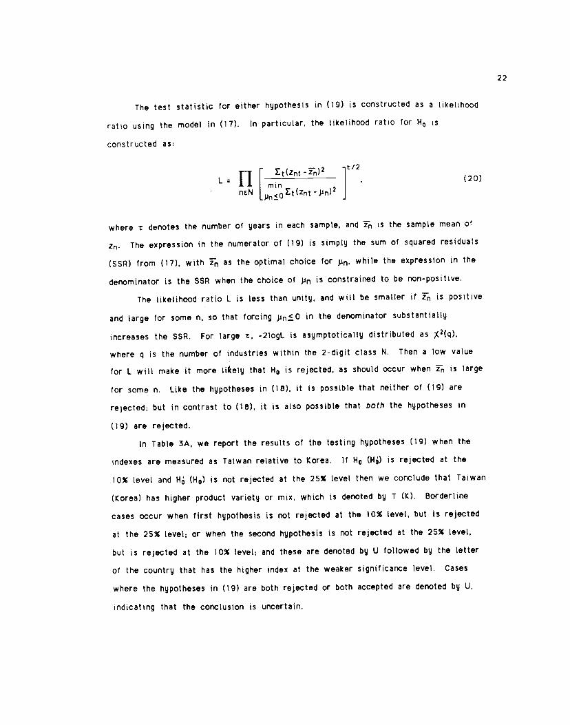
The test statistic for either hypothesis in (19) is constructed as a likelihood

ratio using the model in (1 7). In particular the likelihood ratio for H0 is

constructed as:

TT t(Znt')2 t/2L: . (20)

mm

ncN pn<ot(zntJmn)2

where t denotes the number of years in each sample, and 1n is the sample mean of

Zn. The expression in the numerator of (19) is simply the sum of squared residuals

(SSR) from (17). with 1n as the optimal choice for j.'n' while the expression in the

denominator is the SSR when the choice of .i is constrained to be non-positive.

The likelihood ratio L is less than unity, and will be smaller if is positive

and large for some n. so that forcing in the denominator substantially

increases the SSR. For large t, -2logL is asymptotically distributed as

where q is the number of industries within the 2-digit class N. Then a low value

for L will make it more lifcely that H0 is rejected, as should occur when is large

for some n. Like the hypotheses in (18). it is possible that neither of (19) are

rejected: but in contrast to (18), it is also possible that both the hypotheses in

(19) are rejected.

In Table 3A, we report the results of the testing hypotheses (19) when the

indexes are measured as Taiwan relative to Korea. If H0 (Hi) is rejected at the

1 0% level and H (H0) is not rejected at the 25% level then we conclude that Taiwan

(Korea) has higher product variety or mix, which is denoted by I (K). Borderline

cases occur when first hypothesis is not rejected at the 10% level, but is rejected

at the 25% level: or when the second hypothesis is not rejected at the 25% level,

but is rejected at the 10% level: and these are denoted by U followed by the letter

of the country that has the higher index at the weaker significance level. Cases

where the hypotheses in (19) are both rejected or both accepted are denoted by U,

indicating that the conclusion is uncertain.

22

5. Empirical Results5.1. TaIwan-Korea ComparisonA. Product Variety

The sharpest results tn Table 3 are obtained for the product variety index,

where Taiwan had greater variety in more industries within each 2-digit category

than Korea. In the 5-digit industries, it had higher product variety in 42-44% of

the industries in each period (bottom of Table 3), while Korea showed greater

diversity in only 5-8%. For the other half of the industries, the hypothesis test

was inconclusive.

In the 2-digit results in Table 3A. Taiwan was found to have greater product

variety in 10 industries for the first period and 12 industries for the second, while

Korea did not show greater diversity in any of the industries during both periods.

In addition, when we checked the absolute number of varieties exported, Taiwan

always provided more in every industry across the years, without exception. These

results strongly confirm that Taiwan, with non-vertically-integrated business

groups supplying inputs to'the export sector, provides greater product variety than

the Korean economy. An interpretation of these results is that the small export

firms in Taiwan fill many more market niches than the large, vertically-

integrated business groups in Korea.

B. Product Mix

From the product mix indexes reported in Table 3. we find that Korea

specializes in higher-value final (consumption and capital) goods, while Taiwan

specializes in higher-value intermediate goods. The evidence can be found in the

textile. wood, paper, and metal products industries. In textile mill products. Korea

and Taiwan had their own specialization's in different, but about the same number

of 5-digit industries, which made the 2-digit category uncertain; but Korea had a

clear lead in apparel, which uses the former as the intermediate input and creates

the final products. In the lumber and wood industry. Taiwan was ahead in lumber

23

and wood products for both periods, while Korea was leading in furniture during the

second period. The third example is paper products. Korea and Taiwan had their

own strength in particular materials of paper. paperboard and paper boxes, but Korea

obviously excelled over Taiwan in the printing and publishing industry, which is the

last step to make paper products ready to be consumed. The last case is the metal

products sector. Taiwan had higher product mix in fabricated metal for both

periodsand in primary metal during the first, while Korea led in industrial

machinery.

By dividing industries into intermediate and final products. the respective

specialization's of the two countries becomes more evident. In Table 3, for the

first period, there are 18 intermediate product industries in which Taiwan has

higher product mix, versus seven in Korea; but for final products. Korea had higher

product mix in 37 industries versus 1 7 for Taiwan. Korea moderately increases its

product mix for intermediate goods over time, and in the second period Taiwan has

higher product mix in 19 idustries versus 14 for Korea; while for final products.

Korea had higher product mix in 57 industries and Taiwan in 28. If we check this

finding with the results in Table 3A, all of the 2-digit categories in which Taiwan

had higher product mix are intermediate goods (with the exception of a weak result

in food products), for both the first and the second period. In contrast, Korea has

higher product mix in nearly one-half of the 2-digit final products. with the other

final goods categories being uncertain.

These results of the product mix index can be associated with the business

groups shares in Table 2. After adding up Taiwanese business group and state-owned

shares, there are six industries whose shares are greater than 30% of the total

sales - food (40.7%), textile mill products (50.7%). chemical materials (42.4%),

stone, clay & glass products (47.6%), primary metal (30.7%) and transportation

equipment (39.0%). Except for transportation equipment,23 in all other cases

Taiwan was either ahead or equivalent to Korea in product mix in the first period.

24

even though Korea had similar or even greater business group shares. Taiwan's lead

in some cases was overtaken by Korea in the second period, particularly in food and

primary metal, where Korea had chaebol shares of 33.7% and 28.0%. respectively.

Both of these were higher than the Taiwanese business group shares, but lower than

the sum of the Taiwanese business group and state-owned shares.

Summarizing, the sectors in which Taiwan maintains a lead in product mix

are nearly all intermediate inputs, where it also has high business groups shares.

In contrast, Korea has higher product mix in many final products, where it also has

high cPiaebo! shares. Thus, the presence of business groups in either case appear to

be closely related to the production of high-value product varieties. One

explanation for these results could be that the multiple-output business groups, as

found in both economies, are more concerned with reputation and hence strive for

higher product quality (Rodrik. 1993).

5.2. ComparIson with Japan

Since Korea is less diversified and the comparison above is based on the

products that Korea and Taiwan both exported, the index results reflect Korea's

performance in exports better than Taiwan's. To present the overall performance of

Taiwan, we need a countrywith broader production range as the benchmark, and

Japan is used for that purpose.

A. Variety Index

Japan dominated both Taiwan and Korea in product variety. In the Taiwan-

Japan comparison, among 1 8 2-digit industries (Table 4A, bottom), Japan dominated

in 11 industries in the first period, but Taiwan caught up slightly and narrowed

down Japan's lead to 9 industries in the second period. Taiwan itself had greater

product variety in two cases, and the ranking was inconclusive in seven other

industries in this latter period. The industries in which Taiwan led - lumber and

wood products, leather products, and weakly in food products - were all light

25

industries; four of the other 2-digit industries that could not be ranked with Japan

in variety were also light industries. Japan had greater variety than Taiwan across

nearly all of the heavy industries, however. In addition. Japan had greater product

variety than Korea in all 2-digit industries except leather products (Table 5A).

From our model of section 3. higher product variety is expected from an economy

that is much larger in its resource base, and this is confirmed by the comparison of

either Taiwan or Korea with Japan.

B. Product Mix Index

For the product mix index, reported in Tables 4-5. Taiwan and Korea each led

Japan within some 5-digit industries within most 2-digit categories, and Japan led

in other 5-digit industries. As a result, for the 2-digit hypothesis tests reported

in Tables 4A-5A, neither Taiwan nor Korea could be ranked with Japan in the vast

majority of cases.

Considering the results in Table 3A. during the first period Taiwan had higher

product mix than Japan in chemicals (weakly) and rubber and plastic industries,

but its leads in these two industries were overtaken by Japan in the second period.

In heavy industries. Taiwan had higher product mix only in fabricated metal (second

period), and weakly higher mix during only one period in chemical products and

transportation equipment (consisting or mainly bicycles and parts and auto parts).

For the Korea-Japan comparison in Table 5A, we find that Korea had higher

product mix in some of the light industries - food and leather products - as well as

heavy industries - industrial machinery in the first period, and transportation

equipment. For the latter, Korea had an advantage in selling more higher-value

bicycles and parts, while its auto parts could not be ranked with Japan; automobiles

are not included because Korea did not continuous export them in the full first and

second periods. Generally. Korea leads Japan in product mix only in selected final

goods industries, while Japan leads in a number of the intermediate products.

especially in the second period.

26

6. ConclusionsWe have applied the product variety and mix indexes, derived from the CES

aggregator function, to Korean and Taiwanese exports to the U.S. market. These

indexes were used to test the hypothesis that Taiwan contributed more product

varieties, due to its non-vertically-integrated market structure, and also observe

the differences in product mix. The results presented above strongly confirm the

high product variety of Taiwan relative to Korea. In product mtx, Korea led

especially in final (consumption and investment) goods. while Taiwan led in a

number of intermediate products.

By comparing these results with the business group shares among industries,

it appears that the large scale of the Taiwan business groups in intermediate

products served to facilitate the exporters of the same industries, making these

industries equivalent with Korea in product mix. On the other hand, the integration

of production in Korean chaebol make their final product exports relatively stronger

in product mix than their tntermediate product exports. We feel that these results

confirm the importance of market structure in determining trade patterns, and also

demonstrate the usefulness of using business groups as a measure of market

structure. Business groups of various types are found in many other Asian and

Western countries, and lead to large differences in market structure, as described

by Caves (1989). It can be hoped that these international comparisons may be used

to more fully determine the impact of market structure on international trade, and

on other aspects of economic performance.

27

Footnotes

1 These theories are comprehensively analyzed in Helprnan and Krugman (1985).

2 For example, complete specialization may occur due to technological differencesacross countries, as modeled by Davis (1991).

Indeed, Hummels and Levinsohn (1993) test a key hypothesis from Helpman's modelover a set of OECD countries, and over a set of non-OECD countries for which intra-industry trade should not be important. They find substantial support for the

hypothesis in both sets of countries, suggesting that something other than

monopolistic competition explains the results.

See Granovetter (forthcoming) for a general review of the literature on business

groups. For research on business networks in Asia, see Gerlach (1992). Futatsugi

(1986), Hamilton and Biggart (1988). Orru, Hamilton. and Suzuki (1990), Orru,Biggart and Hamilton (1991). and the papers in Hamilton (1991).

Fung (1991) and Lawrence (1991) have examined the effects of the keiretsu onJapanese trade; see also the papers in Krugman (1991).

6 The chaebol are described in Amsden (1989), Biggart (1991) Hamilton and Biggart(1988), Hamilton. Zeile, and Kim (1990). Kim (1991.1993,forthcorning). Orru,Biggart. and Hamilton (1991). Steers et al. (1989) and Zeile (1991).

' Value-added figures were not available for the other countries in Table 1.

8 This internalization is explored in precise detail in our current research.

9 The literature on business groups in Taiwan is relatively small when comparedwith the literature on the Korean chaebol. However, see Chou (1985), Greenhalgh(1988). Hamilton and Biggart (1966), Hamilton and Kao (1991), and Numazaki(1986.1991).

10 Some of the industries in Table 2 include both intermediate and final goods. suchas pulp & paper, printing & publishing (SIC 26*27) and lumber and wood products(SIC 24*25). In these cases, we have classified the industry according to the

principal output in the country with the largest business group share.

28

11 This is based on current research, which is found in Hamilton, Orru arid Biggart

(unpublished).

12 Hamilton. Zeile and Kim (1989, P. 122). This data is based upon the informationfound in China Credit Information Service (1983).

' The six intermarket groups are Mitsubishi. Mitsui. Sumitomo. Fuyo, DKB. and

Sanwa. while the ten other keiretsu are Tokai Bank, IBJ, Nippon Steel, Hitachi,

Nissan, Toyota, Matsushita, Toshiba-IHI. Yokyu and Seiba.

14 See Levy (1991), Table 9, p. 166.

These notions of personal traits are described in greater detail in the chapters

on Chinese business networks in Hamilton (1991). Also see Hamilton and Kao (1991)

and Hamilton. Biggart,, and Orru (unpublished).

16 For examples of an institutional. social economy explanation for business roupstructures in East Asia, see Gereffi and Hamilton (1992). Hamilton and Biggart(1988) and Whitley (1992).

1 The quantity Xa denotes the total sales of the intermediate input by a non-

integrated firm at the price p:O/(-1). and let Sxb denote the share of total salesaccounted for by one business group. If the business groups charged the same pricefor intermediates as non-integrated firms, then we would have x, :xa(l-sxb), sincexb excludes sales of the input within the group. In fact, the business group will

charge a higher price for the inputs when they produce a positive measure of them.

so that Xb <x3(1 -Sxa). The optimal price for the group is Pb t/(-1), where

is the elasticity of demand for the entire range of inputs produced.

If follows that the profits earned on each unit sold are (pb_i):

(Pa1)/(15xb). Profits over all units are then (pb—l)xb- kx <(Pa_1)Xa_kx:Ttxa.

18 Trade balance in final goods implies LN"(q")1 th/[GNbqt +Naq *N(q*)1i]

,Nq1.N*(q_)1], where the left-side is home

import expenditure and the right-side is home exports. Using this equality in (7).

we immediately obtain (71.

29

Expression (14) follows directly from (13). because total expenditure equals

unit-costs multiplied by output, or E:c(q1,lj)g(yj.I3).

20 From Sato (1976) and Vartia (1976), the formula for this price index is

P(qJ.qk.q.qk.I) . f(Ptj/p)' , where the weights w1(l) are computed using the

lel

expenditure shares of the two countries, as follows: s(l) . qjjyj1/qjjytj.id

( 5;(I)-Sik(l) •\ ( s1(l)—s(I)slk(l) qjkyj/qjyik. and w(l) Ins(l) - lnsik(l)J /

lnsij(l) - lnsik(l)tel tel

The numerator in the definition of w1(1) is a logarithmic mean of StJ and s. andlies between these cost shares. Then the weights w1(l) are a normalized version of

the logarithmic means, and add up to unity.

21 The value and quantity of each 7-digit TSUSA commodity are reported in U.S.Bureau of the Census (1978-88). which was obtained on magnetic tape. The price of

each variety is a unit-valu. computed by dividing total import value by totalquantity at the 7-digit TSUSA level. A concordance file matching TSUSA categorieswith import-based SIC code numbers was used to construct the product groups.

22 An example of a 5-digit SIC category is men's and boy's suits, coats andovercoats.' We also calculated all indexes using the 8-digit SIC as the industrylevel, an example of which is 'men's and boy's suits.' The 5-digit and 8-digit SIClevels gave very similar results for product mix and vareity; see Yang (1993).

23 The transportation industry is a special case in which Taiwanese businessgroups' production is concentrated in automobile manufacturing and state-owned inshipbuilding. most of which is for domestic consumption rather than export.

30

References

Amsden, Alice H (1989) South Korea and Late lndustrtalization. New York: OxfordUniversity Press.

Arrow. Kenneth J. (1969) "The Organization of Economic Activity: Issues Pertinentto the Choice of Market versus Nonmarket Activity," in The Analusts andEvaluation of Public Expenditure: The PPB Sustem, Vol. 1, U.S. Joint EconomicCommittee. 91 st Congress. 1 st Session. Washington. D.C.: GovernmentPrinting Office. 59-73.

Arrow, Kenneth J. (1974) The Limits of Orcanization. New York: W.W. Norton.

Biggart. Nicole Woolsey (1990) "Institutionalized Patrimonialism in KoreanBusiness." In Comparative Social Research 12: 1 13-133.

Caves. Richard E. (1989) "International DIferences in Market Structure." in RichardSchmalensee and Robert D. WiIlig. ed. Handbook of Industiral OrQanization,New York: North-Holland. vol. II. chapter 21.

China Credit Information Service (1983) Business Groups in Taiwan 1983-84. Taipei:China Credit Information Service. Ltd.

Chou, Tein-Chen (1985) Industrial Organization in the Process of EconomicDevelopment: The Case of Taiwan. 1950-1980. Louvain-la-Neuve: UniversiteCatholique de Louvain. Facu!te des Science Ecoriomiques. Sociales et Politiques.

Davis, Donald (1991) Explaining the Volume of Intra-industry Trade: Are IncreasingReturns Necessary?" International Finance Discussion Paper *411. Board of

Governors of the Federal Reserve System. Washington. D.C.

Feenstra, Robert C. (1993) "New Product Varieties and the Measurement of

International Prices." American Economic Review, forthcoming.

Fung, K.C. (1991) "Characteristics of Japanese Industrial Groups and Their PotentialImpact on U.S.-Japanese Trade," in Robert E. Baldwin. ed. Empirical Studiesof commercial Policy. Chicago: Univ. of Chicago and NBER, 137-164.

Futatsugi, Yusaku (1986) JaDanese Enterprise Groups. Kobe, Japan: School ofBusiness. Kobe University.

Gereffi, Gary and Gary G. Hamilton (1992) "The Social Economy of GlobalCapitalism." Paper presented at the annual meetings of the AmericanSociological Association, Pittsburgh. PA, August.

31

Gerlach, Michael (1992) Alliance CaDitalism: The Strategic Organization ofJaDanese Business. Berkeley: University of California Press.

Granovetter, Mark (1985) Economic Action and Social Structure, American Journalof SociolooU 91:481-510.

Granovetter, Mark. Forthcoming. Business Groups. in Neil Smelser and RichardSwedberg (eds.), Handbook of Economic Sociolou. Princeton: PrincetonUniversity Press.

Greenhalgh. Susan (1988) Families and Networks in Taiwan's EconomicDevelopment. Pp. 224-245 in Contending ADDroaches to the Political Econom,jof Taiwan. Edwin Winckler and Susan Greenhaigh (eds.). Armonk. NY: M.E.Sharpe.

Hamilton. Gary G. and Nicole Woolsey Biggart (1988) Market. Culture, andAuthority: A Comparative Analysis of Management and Organization in the FarEast. American Journal of Sociologu, Special Issue on Economic Sociology, 94,July, S52-S94.

Hamilton, Gary G.. William Zeile and Wan-Jin Kim. (1990) The Network Structuresof East Asian Economies in S.R. Clegg and S.G. Redding (eds.). CaDitalism inContrasting Cultures. Berlin: de Gruyter.

Hamilton. Gary G. and Kao Cheng-shu. (1990) The Institutional foundations ofChinese Business: The Family Firm in Taiwan. ComDarative Social Researchvol. 12.

Hamilton, Gary G.. ed. (1991) Business Networks and Economics DeveloDment in Eastand Southeast Asia. Hong Kong: Center of Asian Studies.

Hamilton, Gary G., Nicole Woolsey Biggart. and Marco Orru. Unpublished Manuscript.Network Caojtalism: Economic Organization in Industrial East Asia.

Helpman. Elhanan and Paul Krugman (1985) Market Structure and Foreign Trade.Cambridge: MIT Press.

Helpman, Elhanan (1987) lmperfect Competition and International Trade: Evidencefrom Fourteen Industrial Countries, Journal of the JaPanese and InternationalEconomies 1(1). 62-81.

Helpman. Elhanan and Paul Krugman (1985) Market Structure and Foreign Trade.Cambridge: MIT Press.

32

Hurnmels, David and James Levinsohn (1993) "Product Differentiation as a Source ofComparative Advantage?" American Economic Review. Papers and ProceedlnQs.83(2). May. 445_44g,

Kao. Cheng-shu (1991) "Personal Trust in the Large Businesses in Taiwan, ATraditional Foundation for Contemporary Economic Activities." Pp. 66-76Business Networks and Economic Development in East and Southeast Asia.edited by Gary G. Hamilton. Hong Kong: Center of Asian Studies. University ofHong Kong.

Kim. Eun Mee (1993) "Contradictions and Limits of a Developmental State: WithIllustrations from the South Korean Case." Social Problems (May).

Kim, Eun Mee (1991) "The Industrial Organization and Growth of the Korean ChaebolIntegrating Development and Organizational Theories." in Business Networksand Economic Development in East and Southeast Asia. Gary 6. Hamilton (ed.).Hong Kong: Center of Asian Studies. University of Hong Kong. 272-299.

Kim, Eun Mee. Forthcoming. Bia Business. Strona State: Collusion and Conflict inKorean DeveloDment. 1960-1990. Berkeley: University of California.

Krugman. Paul (1991) Trade With Jaoan. Chicago: Univ. of Chicago and NBER.

Numazaki, Ichiro (1986) "Networks of Taiwanese Big Business." Modern China 12,48 7-534.

Lawrence. Robert 2. (1991) "Efficient or Exciusionist? The Import Behavior ofJapanese Corporate Groups." Brooina PaDers on Economic Activitu, 311 -341.

Levy. Brian (1991) "Transactions Costs, The Size of Firms and Industrial Policy."Journal of Develoment Economics 34. 151 -1 76.

Numazaki, Ichiro (1991) "The Role of Personal Networks in the Making of Taiwan'sGuanxiqiye (Related Enterprises)." pp. 77- 93 in Business Networks andEconomic Develooment in East and Southeast Asia. edited by Gary G. Hamilton.Hong Kong: Center of Asian Studies, University of Hong Kong.

Orru, Marco, Gary G. Hamilton, and Mariko Suzuki (1990) "Patterns of Inter-FirmControl in Japanese Business." Organizational Studies 10(4), 549-574.

Orru, Marco, Nicole Woolsey Biggart, and Gary G. Hamilton, (1991) "OrganizationalIsomorphism in East Asia: Broadening the New Institutionalism," in WaIterW. Powell and Paul J. DiMaggio (eds.). The New Institutionalism inOrganizational Analusis, Chicago: Univ. of Chicago Press.

33

Powell. Walter W. (1990) Neither Market Nor Hierarchy: Network Forms orOrganization. Research in Organizational Behavior. 12: 295-336.

Rodrik. Dani (1993) industnal Organization and Product Quality: Evidence fromSouth Korean ad Taiwanese Exports. in Paul Krugman and Alasdair Smith. eds.,ErnDirical Studies of Strategic Trade Policy. Chicago: Univ. of Chicago andNBER.

Sato, Kazuo (1976) The Ideal Log-change Index Number. Review of Economics andStatistics 58. May. 223-228.

Steers. Richard H.. Yoo, Keun Shi. and Gerardo Lngson (1989) The Chaebol: KpreasNew Industrial Might. New York: Harper and Row.

Vartia, Yrjo 0. (1976) ideal Log-change Index Numbers, Scandinavian Journal pfStatistics 3, 121-126.

Whitley. Richard (1992) Business Sustems in East Asia. London: Sage.

Williamson, Oliver E. (1975) Markets and Hierarchies. New York: The Free Press.

Williamson, Oliver E. (1985) The Economic Institutions of CaDitalism. New York:The Free Press.

Wong. Siu-Lun (1985) The Chinese Family Firm: A Model. British Journal orSociology 36. 58-72.

Yang, Tzu-Han (1993) industriaL Structure and Trade Patterns: Evidence from SouthKorea and Taiwan. Ph.D. Dissertation. University of California. Davis.

Zeile, William (1991) industrial Policy and Organizational Efficiency: The KoreanChaebol Examined. in Gary G. Hamilton (ed.) Business Networks and EconomicsDeveloDment in East and Southeast Asia. Hong Kong: Center of Asian Studies.

U.S. Bureau of the Census (1976-88) U.S. General Imoorts for Consumotion.Schedule A. FT1 35. Commodity by Country. Washington. D.C.: U.S. Department orCommerce. Government Printing Office.

34

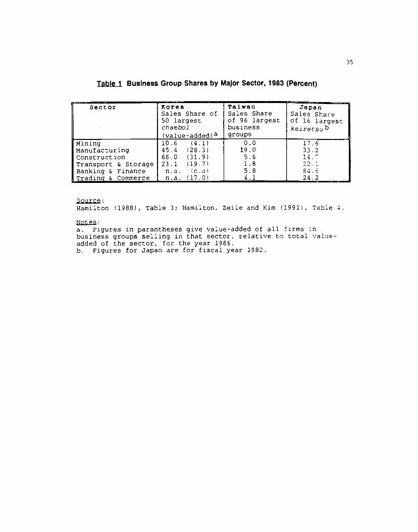
Table 1 BusIness Group Shares by Major Sector, 1983 (Percent)

Sector

.

oreaSales Share of50 largestchaebol(valueadded)a

TaiwanSales Shareof 96 largestbusinessgroups

JapanSales Shareof 16 largestkeiretsub

MiningManufacturingConstructionTransport & StorageBanking & FinanceTrading & Commerce

10.6 (4.1)45.4 (28.3)66.0 (31.9)23.1 (19.7)n.a. (n.a)n.a. (17.0)

0.019.05.61.85.84.1

17.633.214.22.184.524.2

Source:Hamilton (1988), Table 3; Hamilton, Zeile and Kim (1991), Table 4.

Notes:a. Figures in parantheses give value-added of all firms inbusiness groups selling in that sector, relative to total value-added of the sector, for the year 1986.b. Figures for Japan are for fiscal year 1982.

35

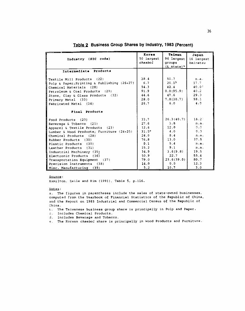
Table 2 Business Group Shares by Industry, 1983 (Percent)

Kor•a Taiwan JapanIndustry (SIC cod.) 50 largest 96 largest 16 largest

chaebol groups keiretsu

-___________ (& state)3

int.rm.diat. Product.

Textile Mill Products (22) 38.4 50.7 n.a.

Pulp & Paper;Printing & Publishing (26+27) 6.7 20lb 17.Chemical Materials (28) 54.3 42.4 40.0

Petroleum & Coal Products (29) 91.9 0.0(95.9) 40.2

Stone. Clay & Glass Products (32) 44.6 47.6 29.0

Primary Metal (33) 28.0 7.8(30.7) 58.1

Fabricated Metal (34) 26.7 6.0 4.0

Final Products

Food Products (20) 33.7 26.3(40.7) l8.2Beverage & Tobacco (21) 27.6 3.8 na.Apparel & Textile Products (23) 12.6 12.0 0.0

Lumber & Wood Products; Furniture (24+25) 315e 4.0 0.0

Chemical Products (28) 24.0 8.4 n.a.

Rubber Products (30) 76.8 13.0 37.5

Plastic Products (30) 0.1 5.4 n.a.

Leather Products (31) 15.2 9.1 n.a.

Industrial Machinery (35) 34.9 3.6(9.8) 19.5

Electronic Products (36) 50.9 22.7 55.4

Transportation Equipment (37) 79.0 23.6(39.0) 80.7

Precision Instruments (38) 14.0 0.0 12.3

Misc. Manufacturing (39) 5.2 10.7 3.0

Source:

Hamilton, Zeile and Kim (1991), Table 5, p.116.

Notes:

a. The figures in parentheses include the sales of state-owned businesses,computed from the Yearbook of Financial Statistics of the Republic of China,and the Report on 1983 Industrial and Commercial Census of the Republic ofChina.b. The Taiwanese business group share is principally in Pulp and Paper.

Includes Chemical Products.ci. Includes Beverage and Tobacco.. The Korean chaebol share is principally in Wood Products and Furniture.

36

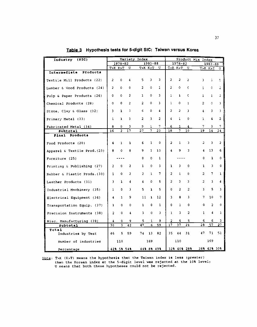
Table 3 Hypothesis tests for 5-digit SIC: Taiwan versus Korea

Industry (SIC) Variety Index Product Mjx Index1978—82 1983—88 1978—82 1983-88

T>K K>T U T>K K>T U T>K K>T U T>K K>T UInt.rm.diat. Products

Textile Mill Products (22)

Lumber & Wood Products (24)

Pulp & Paper Products (26)

Chemical Products (28)

Stone, Clay & Glass (32)

PrimaryMetal(33)

Fabricated Metal (34)

2 0 4 5 3 3

2 0 0 2 0 1

0 0 2 1 0 3

0 0 2 2 0 3

3 1 3 6 0 4

1 1 3 2 3 2

8 0 3 9 1 7

2 2 2 3 3

2 0 0 1 0 2

1 3. 0 1 1 2

1 0 1 2 0 3

2 2 3 4 3 3

4 1 0 1 4 2

6 1 4 7 3 7

Subtotal 16 2 17 27 7 23 18 7 10 19 14 24Final Products

Food Products (20)

Apparel & Textile Prod. (23)

Furniture (25)

Printing & Publishing (27)

Rubber & Plastic Prods.(30)

Leather Products (31)

Industrial Machinery (35)

Electrical Equipment (36)

Transportation Equip. (37)

Precision Instruients (38)

Misc. Manufacturing (39)

4 1 1 6 1 0

8 0 8 9 1 13

—--- 0 0 1

2 0 2 1 0 3

1 0 2 2 1 7

3 1 4 4 0 5

1 0 3 5 1 5

4 1 9 11 1 12

1 0 0 1 0 1

2 0 4 3 0 3

4 0 9 5 1 9

2 1 3 2 3 2

4 9 3 4 13

-——- 0 1 0

1 3 0 1 3 0

2 1 0 2 7 1

2 3 3 2 3 4

0 2 2 3 5 3

3 8 3 7 10 7

0 1 0 0 2 0

1 3 2 1 4 1

2 6 5 6 6 3

Subtotal 30 3 42 47 6 59 17 37 21 28 57 27Total

Industries by Test

Number of industries

Percentage

46 5 59 74 13 82

110 169

42% 5% 54% 44% 8% 49%

35 44 31 47 71 51

110 169

32% 40% 28% 28% 42% 30%

j: T>K (K>T) means the hypothesis that the Taiwan index is less (greater)than the Korean index at the 5-digit level was rejected at the 10% level;U means that both these hypotheses could not be rejected.

37

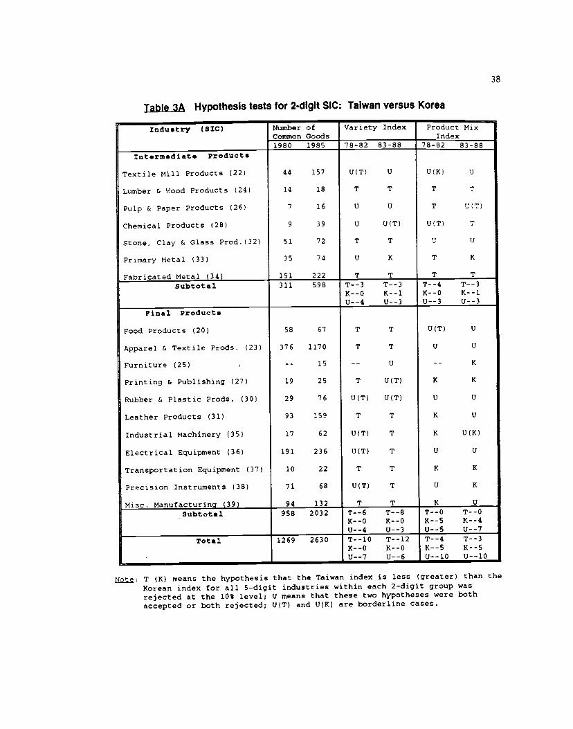
Table_3A Hypothesis tests for 2-digit SIC: Taiwan versus Korea

Industry (SIC) Number ofConsnon Goods

Variety Index Product MixIndex

1980 1985 78—82 83-88 78-82 83-88

Int.rmsdiats Products





Stone, Clay & Glass Prod. 32)

Primary Metal (33)


44 157

14 18

7 16

9 39

51 72

35 74

151 222

U(T( U

T T

U U

U U(T)

T T

U K

T T

U(K) U

T T

T U(T)

U(T) T

U U

T K

T T

Subtotal 311 598 T--3 T--3K--0 K--iU--4 U--3

T--4 T--3K--0 K--iU--3 U--3

Final Products

Food Products (20)

Apparel & Textile Prods. (23)

Furniture (25)


Rubber & Plastic Prods. (30)




Transportation Equipment (37)

Precision Instruments (38)


58 67

376 1170

-- 15

19 25

29 76

93 159

17 62

191 236

10 22

71 68

94 132

T T

T T

-- U

T U(T)

U(T) U(T)

T T

U(T) T

U(T) T

T T

U(T) T

T T

U(T) U

U U

-- K

K K

U U

K U

K U(K)

U U

K K

U K

K USubtotal 958 2032 T--6 T--8

K--0 K--0U--4 U--3

T--0 T--0K--S K--4U--S U--i

Total 1269 2630 T-—i0 T--l2K--0 K--0U--i U--6

T-—4 T-—3K--S K--SU--b U--b

Ng: T (K) means the hypothesis that the Taiwan index is less (greater) than theKorean index for all S-digit industries within each 2-digit group wasrejected at the 10% level; U means that these two hypotheses were bothaccepted or both rejected; U(T) and U(K) are borderline cases.

38

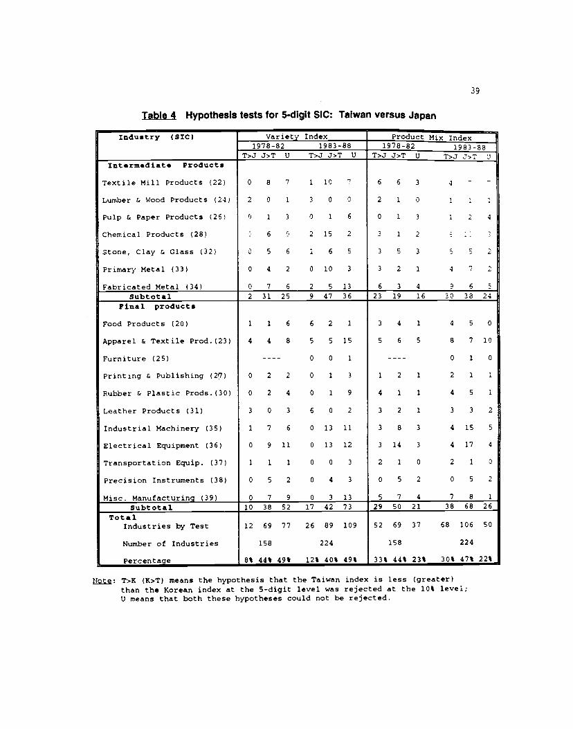
Table 4 Hypothesis tests for 5-digit SIC: Taiwan versus Japan

Industry (SIC) Variety Index Product Mix Index1978-82 1983—88 1978-82 1983-88

T>J J>T U T>J J>T U T>J J>T U T>J J>T UInt.rm.diats Products



pulp & Paper Products (26



PrimaryMetal(33)


0 8 7 1 10

2 0 1 3 0 0

0 1 3 0 1 6

C 6 0 2 15 2

0 5 6 1 6 S

0 4 2 0 10 3

0 7 6 2 5 13

6 6 3 4- —

2 1 0 1

0 1 3 1 2 4

3 1 2 1

3 5 3 5 5 2

3 2 1 4 7 2

6 3 4 9 6 5

Subtotal 2 31 25 9 47 36 23 19 16 30 38 24Final products

Food Products (20)


Furniture (25)








Misc. Manufacturing (39)Subtotal

1 1 6 6 2 1

4 4 8 5 5 15

--—- 0 0 1

0 2 2 0 1 3

0 2 4 0 1 9

3 0 3 6 0 2

1 7 6 0 13 11

0 9 11 0 13 12

1 1 1 0 0 3

0 5 2 0 4 3

0 7 9 0 3 13

3 4 1 4 S 0

5 6 5 8 7 10

---- 0 1 0

1 2 1 2 1 1

4 1 1 4 5 1

3 2 1 3 3 2

3 8 3 4 15 5

3 14 3 4 17 4

2 1 0 2 1 0

0 5 2 0 5 2

5 7 4 7 8 1

10 38 52 17 42 73 29 50 21 38 68 26Total

Industries by Test

!4umber of Industries

Percentage

12 69 77 26 89 109158 224

8% 44% 49% 12% 40% 49%

52 69 37 68 106 50

158 224

33% 44% 23% 30% 47% 22%

j: T>K (K>T) means the hypothesis that the Taiwan index is less (greater)than the Korean index at the 5-digit level was rejected at the 10% level;U means that both these hypotheses could not be rejected.

39

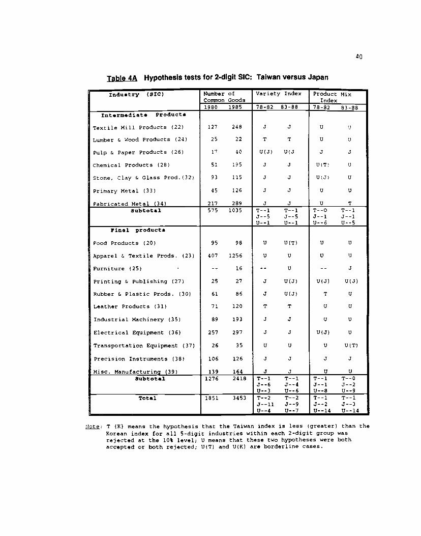
Table 4A Hypothesis tests for 2-digit SIC: Taiwan versus Japan

Induitry (SIC) Number ofCommon Goods


1980 1985 78—82 83—88 78-82 83-88Int.rm.diat• Products





Stone, Clay & Glass Prod.(32)

Primary Metal (33)


127 248

25 22

11 40

51 195

93 115

45 126

217 289

J

T T

U(J) U(J

J J

3 j

3 j

J J

u

U

3 j

U(Tj U

u

u u

U TSubtotal 575 1035 T--1 T--1

J--5 3--SU--i U--i

T--O T--l3--i 3--iU--6 U--S

Final product.

Food Products (20)

Apparel & Textile Prods. (23)

Furniture (25)


Rubber & Plastic Prods. (30)







95 98

407 1256

-- 16

25 27

61 86

71 120

89 193

257 297

26 35

106 126

139 164

U U(T)

U U

-- U

3 U(J)

3 U(J)

T T

3 3

3 3

U U

3 3

3 3

U U

U U

-- 3

U(J) U(J)

T U

U U

U U

U(J) U

U U(T)

3 J

U USubtotal 1276 2418 T--i T--i

3--6 J--4'J--3 U--6

T--1 T--03--i J--2U--8 U--9

Total 1851 3453 T--2 T--23--li J--9U-—4 U--7

T--l T--lJ--2 3--3U--14 U--14

T (K) means the hypothesis that the Taiwan index is less (greater) than theKorean index for all 5-digit industries within each 2-digit group wasrejected at the 10% level; U means that these two hypotheses were bothaccepted or both rejected; U(T) and U(K) are borderline cases.

40

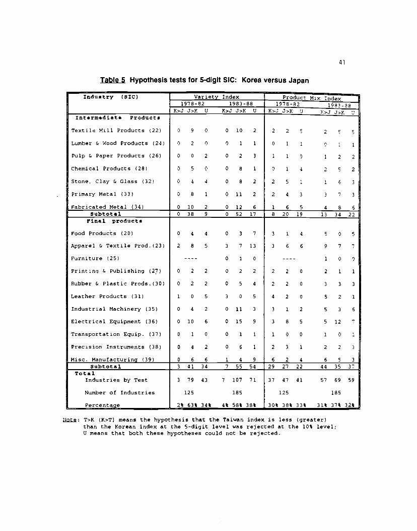
Table 5 HypothesIs tests for 5-digit SIC: Korea versus Japan

Industry (SIC) Variety Index Product Mix Index1978—82 1983-88 1978-82 1983-88

K>J J>Y. TJ K>J J>K U K>J J>K U >j j>y 'Int.rin.diat. Products

Texti1 Mill Products (22)





PrimaryMetal(33)


0 9 0 0 10 2

0 2 0 0 1 1

0 0 2 0 2 3

0 5 0 0 8 1

0 4 4 0 8 2

0 8 1 0 11 2

0 10 2 0 12 6

2 2 5 2 5

0 1 1 0 1 1

1 1 0 1 2 2

0 1 4 2 5 2

2 5 1 1 6 3

2 4 3 3 7 3

1 6 5 4 8 6Subtotal 0 38 9 0 52 17 8 20 19 13 34 22

Final productsFood Products (20)


Furniture (25)









0 4 4 0 3 7

2 8 5 3 7 13

-—-- 0 1 0

0 2 2 0 2 2

0 2 2 0 S 4

1 0 5 3 0 5

0 4 2 0 11 3

0 10 6 0 15 9

0 1 0 0 1 1

0 4 2 0 6 1

0 6 6 1 4 9

3 1 4 5 0 5

3 6 6 9 7 7

---- 1 0 0

2 2 0 2 1 1

2 2 0 3 3 3

4 2 0 S 2 1

3 1 2 5 3 6

3 8 5 5 12

1 0 0 1 0 1

2 3 1 2 2 3

6 2 4 6 5 3

Subtotal 3 41 34 7 55 54 29 27 22 44 35 37Total

Industries by Test

Number of Industries

Percentage

3 79 43 7 107 71

125 185

2% 63% 34% 4% 58% 38%

37 47 41 57 69 59

125 185

30% 38% 33% 31% 37% 32%

jg: T>K (K>T) means the hypothesis that the Taiwan index is less (greater)than the Korean index at the S-digit level was relected at the 10% level;U means that both these hypotheses could not be rejected.

41

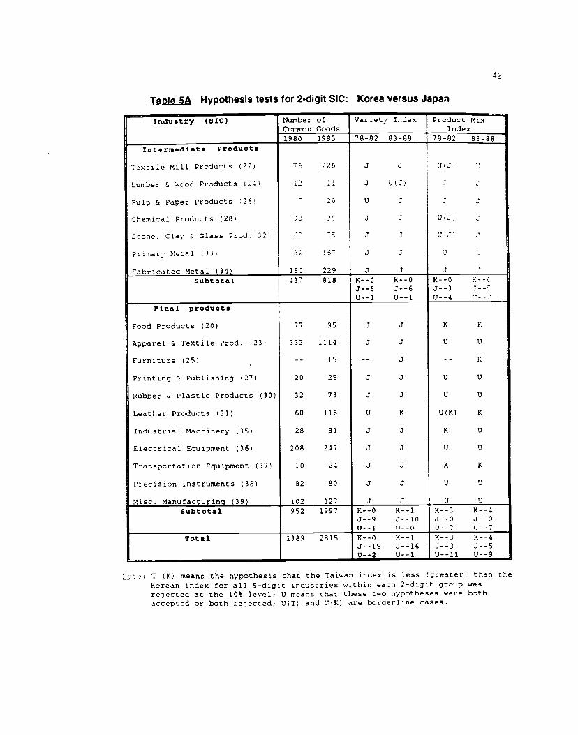
1eA Hypothesis tests for 2-digit SIC: Korea versus Japan

Industry (SIC) Number ofCommon Goods


1980 1985 78-82 83-88 78-82 33-38Int.r.diat• Products


Lumber & wood Products (24)

Pulp & Paper Ptoducts 26

Chemical Products (28>

Stone. Clay & Glass Prod.32)

Prrnary Metal (33)


76 226

12 11

20

33 90

32 l616) 229

.3 .3

.3 tJ(J)

U .3

.3 J

J J

.3 .3

.3 .3

.3 -

.3 .3

U)J)

UJn

.3 .3

Subtotal 337 818 K--0 K--0J--6 J--6U--i U--i

K--0 --0.J--3 .3- -U--4 .Y--2

Final products

Food Products (20)

Apparel & Textile Prod. (23>

Furniture (25)

Printing & Publishing >27)

Rubber & Plastic Products (30)







77 95

333 1114

-- 15

20 25

32 73

60 116

28 81

208 247

10 24

82 80

102 127

J .3

.3 .3

-- .3

.3 .3

.3 .3

U K

.3 .3

.3 .3

.3 .3

.3 J

.3 J

K K

U U

-- K

U U

U U

U(K) K

K U

U U

K K

U U

U U

Subtotal 952 1997 K--0 K--iJ--9 J--10U--i U--0

K--3 K--4J--0 J--0U--7 U--7

Total 1389 2815 K--0 K--i.3—-iS .J--16U--2 U--i

K--3 K--4J--3 j--5U--li U--9

T (K) means the hypothesis that the Taiwan index is less (greater) than theKorean index for all 5-digit industries within each 2-digit group wasrejected at the 10% level; U means that these two hypotheses were bothaccepted or both rejected; U(T) and t)K) are borderline cases.

42

Documents

NBER WORKING PAPER SERIES MARKET … · NBER WORKING PAPER SERIES MARKET STRUCTURE AND INTERNATIONAL TRADE: BUSINESS GROUPS IN EAST ASIA Robert C. Feenstra Tzu-Han Yang Gary G. Hamilton