NBER WORKING PAPER SERIES

MONEY IN A THEORY OF BANKING

Douglas W. DiamondRaghuram G. Rajan

Working Paper 10070http://www.nber.org/papers/w10070

NATIONAL BUREAU OF ECONOMIC RESEARCH1050 Massachusetts Avenue

Cambridge, MA 02138October 2003

We are grateful for financial support from the National Science Foundation and the Center for Research onSecurity Prices. Rajan also thanks the Center for the Study of the State and the Economy for financial support.We thank John Cochrane, Jeff Lacker, Jeremy Stein, and Elu Von Thadden for helpful conversations on thistopic and seminar participants at Berkeley, the Federal Reserve Bank of Richmond, Harvard, Maryland,Stanford, Urbana Champaign, and Utah. The views expressed herein are those of the authors and notnecessarily those of the National Bureau of Economic Research.

©2003 by Douglas W. Diamond and Raghuram G. Rajan. All rights reserved. Short sections of text, not toexceed two paragraphs, may be quoted without explicit permission provided that full credit, including ©notice, is given to the source.

Money in a Theory of BankingDouglas W. Diamond and Raghuram G. RajanNBER Working Paper No. 10070October 2003JEL No. G2, E5, E4, E3

ABSTRACT

We explore the connection between money, banks, and aggregate credit. We start with a simple"real" model without money, where banks make loans repayable in goods and depositors hold claimson the bank payable on demand in goods. Aggregate production may be delayed in the economy.If so, we show that the level of ongoing bank lending, and hence of aggregate future output, candecrease with increases in the real repayment due on deposits: ceteris paribus, the higher the amountdue, the more likely there will be insufficient goods, given the delay, to pay depositors, and the morenew lending has to be curtailed to make up the shortfall. Thus a temporary delay in production canbe exacerbated by banks into a more permanent reduction of total output. A number of inefficienciesincluding bank failures can result if deposits turn out to be too high. We then introduce money inthis model. We show that if demand deposits are repayable in money rather than in goods, banks canbe hedged against production delays: under certain circumstances, the price level will rise withdelays in production, reducing the real value of the deposits banks have to pay out. But demanddeposits payable in money can expose the banks to new risks: the value of money can fluctuate forreasons other than delays in aggregate production. Because deposits are convertible into money ondemand, a temporary rise in money demand immediately boosts the interest rate banks have to paydepositors, which in turn boosts the real amounts banks have to repay them. This increase in the realdeposit burden can again lead to the curtailment of bank lending and even bank failures. The wayto combat these contractionary effects is to infuse more money into the banking system. Our analysisthus makes transparent how changes in the supply of money can work through banks to affect realeconomic activity, without invoking sticky prices, reserve requirements, or deposit insurance. It alsosuggests how bank failures could lead to a fall in prices and a contagion of bank failures, asdescribed by Friedman and Schwartz (1963).

Douglas W. DiamondGraduate School of BusinessUniversity of Chicago1101 East 58th StreetChicago, IL 60637and NBERdouglas.diamond@gsb.uchicago.edu

Raghuram RajanInternational Monetary FundResearch Department, Rm 10-700700 19th Street, N.W.Washington, DC 20431and NBERraghuram.rajan@gsb.uchicago.edu

1

What is the connection between money, banks, and aggregate credit? When can

expansionary monetary policy lead to expanded bank credit? And when can monetary policy help

avert bank failures? These are the questions that motivate this paper.

We start with a “real” model where all contracts are denominated in goods. A bank is an

intermediary, which has special skills that enable it to lend to firms that are hard to collect from.

The bank finances these loans by issuing demandable claims. In Diamond and Rajan (2001), we

show why such an arrangement allows banks to fund potentially long term projects while

allowing investors to consume when needed.

Unfortunately, demandable claims expose the banking system to real shocks that create a

mismatch between the production of consumption goods and the real amount promised to the

depositors. Even if the shortage of consumption goods, also termed a real “liquidity shortage”, is

merely due to delay in production and not because of any reduction in the production possibilities

of the economy, it can be amplified by the banking system. Banks will cut short long term

projects, that is, curtail credit. Banks may fail even if depositors have the most optimistic beliefs

possible (unlike, say, in models like Diamond and Dybvig (1983)).

All this is shown in an economy where all contracts, including demand deposits, are

denominated in goods. The repayment on deposits is assumed fixed over the next instant and,

because of difficulties in contracting, cannot be an explicit function of realizations of individual

bank or detailed aggregate conditions. In practice, however, bank deposits and loans typically

promise to repay money, not goods -- though deposits are denominated in foreign currencies in

some countries, which essentially makes them real from the perspective of that country’s citizens.

What would happen if deposit contracts were instead nominal, that is, denominated and repayable

in domestic currency? Would the system smooth real shocks?

To examine this, we focus on two sources of value for money. First, money, and any

maturing government liability, is a claim on the government and may have intrinsic value from

the ability of citizens to pay taxes with it. Second, money, specifically currency, facilitates

transactions; Some goods may be sold only for cash as in cash-in-advance models (see Clower

2

[1967] and Lucas-Stokey [1987]). Examples are illegal goods like drugs, services that are sold in

transactions where the seller seeks to keep his identity hidden from tax authorities, or goods

encountered serendipitously where the relative cost of establishing a credit transaction may be too

high. Depending on circumstances, the “fiscal” value of money may exceed or be dominated by

its “transactions” value.

Suppose now that banks issue nominal deposits. To the extent that the real value of a unit

of money falls when the current aggregate supply of goods is low, deposits denominated in

money offer banks a natural hedge by adjusting effective real demand to supply. And there are

reasons why this might happen – the present value of taxes on production falls if production is

delayed so the fiscal value of money falls. Similarly, it is plausible that transactions fall when

aggregate production is delayed so the transactions value of money could also fall. If the

quantities of currency and bonds are fixed, the real value required to be paid out on nominal

deposits will then fall in consonance with an adverse shock to the supply of goods, reducing the

liquidity shortage and its effects on, and via, the banking system.

However, perfect state contingent adjustment of liquidity demand using nominal deposit

contracts is a fairly special idealization. More generally, the transactions value of money may

have large variation that is independent of aggregate production.1 If so, banks that issue nominal

demandable deposits are particularly vulnerable: if cash goods are temporarily cheap (for

example, because the supply of money is low relative to available cash goods) banks will be

forced to increase interest rates offered on demandable deposits to keep depositors from

withdrawing. In turn, this will increase the real repayment obligations of the banks, potentially

even causing bank failures. When the value of money is not “well-behaved”, far from reducing

aggregate real liquidity demand when aggregate supply falls, nominal deposits may actually

increase it, exacerbating real liquidity shortages, and reducing credit.

1 If illegal goods and informal services require cash-in-advance, there is no reason they should be positively correlated with aggregate formal production. In fact, if more workers lose formal employment and enter the informal sector, there could be a case for arguing for negative correlation between aggregate production and cash transactions. Similarly, if a temporary downturn prompts asset sales, a negative correlation could again emerge.

3

Monetary intervention could play a useful role here by making the value of money

correspond better to aggregate real liquidity conditions. By increasing the money supply

available for transactions when the transactions demand is high (and by committing to provide

monetary support in the future when needed), the monetary authority offsets aberrant monetary or

real shocks and keeps the price level stable. This limits depositor incentives to withdraw and the

future real repayment obligations of banks. Banks then will respond by continuing, rather than

curtailing, credit to long-term projects, thus increasing aggregate economic activity.

Our view of the monetary transmission mechanism could then be termed a version of the

bank lending channel view (see Bernanke and Gertler (1995) or Kashyap and Stein (1997) for

comprehensive surveys) but with a difference. According to the traditional lending channel view,

monetary policy affects bank loan supply, which in turn affects aggregate economic activity.

Three assumptions have been thought to be key to the centrality of banks in the transmission

process: (i) binding reserve requirements tie the issuance of bank demand deposits to the

availability of reserves (ii) banks cannot substitute between demand deposits and other forms of

finance easily so they have to cut down on lending when the central bank curtails reserves (iii)

client firms cannot substitute between bank loans and other forms of finance, so they have to cut

down on economic activity.

The concern with the traditional view of the bank lending channel is that as reserve

requirements have been eliminated for almost all bank liabilities except demand deposits, the

argument that banks will find it difficult or expensive to raise alternative forms of financing to

demand deposits becomes less persuasive -- see, for example, the critique by Romer and Romer

(1990), though see Stein (1998) who argues that demand deposits are still special because they

are insured. But there does seem to be strong evidence that monetary policy has effects on bank

loan supply (Kashyap, Stein, and Wilcox (1995), Ludvigson (1998)), has greater effect on banks

at times when their balance sheets look worse (Gibson (1996)) and has the greatest effect on the

policies of the smallest and least liquid banks (Kashyap and Stein (2000)).

4

In contrast to traditional models of the lending channel, our model does not rely on

reserve requirements or on deposit insurance, or even on sticky prices. An expansionary open

market operation (buying bonds with money) increases financial liquidity, decreases the real

value that banks must pay in the future to retain deposits in the present, which alleviates the real

liquidity demands on banks, which then allows them to fund more long-term projects to fruition.

These effects will be most pronounced for constrained banks in bad times. Thus it is perhaps best

to term ours the liquidity version of the lending channel of transmission.

The rest of the paper is as follows. In section I, we describe the framework, in section II

we describe the problems with real deposit contracts and the circumstances under which nominal

contracts can improve upon them. In section III, we introduce money and examine how aggregate

activity and bank credit is affected by shortages of real and financial liquidity. In section IV we

examine how monetary policy is transmitted in our model and then we conclude.

I. The Framework

1.1. Agents, Assets, Endowments, Preferences, Technology.

Consider an economy with four types of risk neutral agents: investors, entrepreneurs,

bankers, and dealers, a date when contracts are written and five future dates: 0, 1, 2, 3, and 4.

Dates 1 and 3 are event rather than calendar dates, and are best assumed close in calendar time to

dates 2 and 4 respectively.

There are goods, and financial assets consisting of cash and government bonds. Only

investors are initially endowed with resources. Each investor has one unit of good, M0 of cash,

and B2 face value of government bonds maturing at date 2 (a table of notation is on page 40 in the

appendix).2 When the bonds mature, the government extinguishes them by repaying their face

value in new money or issuing fresh bonds maturing at date 4.

Investors are impatient in that their utility is only the sum of consumption on, or before,

date 2. Because all consumption on or before date 2 is perfectly substitutable, we will refer to all

2 Because we have three calendar dates in the model, 0,2,and 4, a bond maturing at date 2 is a one period (short term) bond. We do not consider long term bonds in this paper.

5

such consumption as early consumption. All other agents also get equal utility from consumption

after date 2 (late consumption), so their utility is the sum of early and late consumption. The

impatience of investors limits the response of consumption demand to interest rates (equivalently,

it limits the substitutability of consumption across time), which is needed for liquidity to matter.

Each entrepreneur has a project, which requires the investment of a unit of good before

date 0. It produces C in goods at date 2 if the project is early or C at date 4 if the project is

delayed and produces late. Alternatively, goods can be stored at a gross real return of 1. We

assume that there is a shortage of endowments of goods initially relative to projects that can be

invested in. Let the gross real interest rate between date j and date k be rjk and the gross nominal

interest rate be ijk .

1.2. Projects and the non-transferability of skills The primary friction underlying the model is that those with specific skills cannot commit

to using their human capital on behalf of others, that is, they cannot commit to repay all the value

they generate to outsiders. Creditors will lend only to the extent that they can compel borrowers

to repay -- either by threatening to seize the borrower’s assets and generate value with them or by

committing to harm the borrower if the borrower defaults.

Specifically, since entrepreneurs have no endowments, they need to borrow to invest.

Each entrepreneur has access to a banker who has, or can acquire during the course of lending,

knowledge about an alternative, but less effective, way to run the project. The banker’s specific

knowledge allows him to (make the credible threats that will enable him to) collect γC from an

entrepreneur whose project just matures. No one else has the knowledge to collect from the

entrepreneur. 3 Because the entrepreneur’s skills are critical to the project, the project is illiquid in

that the entrepreneur can pay at most Cγ of the C that he generates.

Regardless of whether a project is early or late, the banker can also restructure the project

at any time to yield c in early consumption goods – intuitively, restructuring implies stopping half

finished projects and salvaging all possible goods from them. We assume 3 For a relaxation of these assumptions, see Diamond and Rajan (2001).

6

1c C Cγ< < < , (1.1)

Since no one other than the bank has the specific skills to collect from the entrepreneur, the loan

to the entrepreneur is also illiquid in that the banker will get less than γC if he has to sell the loan

before the project matures. Any buyer will realize that the banker will extract a future rent for

collecting the loan, and the buyer will reduce the price he pays for the loan accordingly. In fact,

bank loans are so dependent on the banker’s specific skills for collection that the banker prefers

restructuring projects to selling them.4 The illiquidity of both projects and bank loans stems from

the inalienability of human capital (see Hart and Moore (1994)).

Given the shortage of endowment relative to projects, competition will force the select

few entrepreneurs who get a loan to promise to repay the maximum possible on demand, γC, to

obtain the loan. This simplifying assumption is relaxed later.

1.3. Financing Banks

Since bankers have no resources initially, they have to raise them from investors. But

investors have no collection skills (and, consequently, bank loans are worthless in their hands), so

how do banks commit to repaying investors? By issuing demand deposits! In our previous work

(Diamond and Rajan (2000, 2001)), we argued that the demandable nature of deposit contracts

introduces a collective action problem for depositors that makes them run to demand repayment

whenever they anticipate the banker cannot, or will not, pay the promised amount. Runs destroy

the banker’s rents. Because depositors are committed to harming the banker if he reneges on his

promise to pay, the banker will repay the promised amount on deposits whenever he can.

Deposit financing introduces rigidity into the bank’s required repayments. Ex ante, this

enables the banker to commit to repay if he can (that is, avoid strategic defaults by passing

through whatever he collects to depositors). However, it exposes the bank to destructive runs if he

truly cannot pay (it makes non-strategic default more costly): when depositors demand repayment

4 See Diamond and Rajan (2005) for the easily satisfied conditions that lead to this outcome.

7

before projects have matured and the bank does not have the means of payment, it will be forced

to restructure projects to get c immediately instead of allowing them to mature and generate γC.

All banks face a perfectly competitive deposit market where deposits flow freely to any

bank that can credibly repay the market clearing rate of return.

1.4. Uncertainty

Each bank faces an identical pool of entrepreneurs before date 0. At date 0, the state s is

realized and the banks become differentiated. A bank could turn out to be type G with all

entrepreneurs having early projects or type B with ,B sα < 1 entrepreneurs with early projects. The

fraction of banks of type G in state s is ,G sθ . In what follows, we will suppress the dependence on

the state for notational convenience. Also, instead of introducing the whole model at one go, we

will introduce the essential features of the “real’ model, leaving the details of money for later.

1.5. Timing.

Before date 0.

Investors deposit goods in competitive banks in return for claims that make them better off in

expectation than storage.5 Let us start by assuming that banks issue real deposits, that is, each

bank offers to repay d0 early consumption goods (or claims of equivalent value) on demand for

the resources they get from each identical investor. Banks lend the goods to entrepreneurs in

5 While we have made assumptions here forcing the investor to lend via the bank, we show in Diamond and Rajan (2001) that banks and their fragile liability structures arise endogenously to facilitate the flow of credit from investors with uncertain consumption needs to entrepreneurs who have hard-to-pledge cash flows. If investors lent directly, acquired collection skills, but wanted to consume at an interim date, they would have to sell their loans at a huge discount. Far better to hold demand deposits on a bank and let the bank acquire the collection skills. If the investor wants to consume at an interim date, the bank will repay him and refinance by borrowing from others (early entrepreneurs) who have a surplus. In this way, the bank does not interrupt the late, but valuable, project while also allowing the investor to consume a larger amount when he desires consumption. One might also ask if the entrepreneur can replicate the banker’s ability to commit by issuing demand deposits. The answer is no, because the banker’s human capital is essential only in making transfers (between the entrepreneur and the depositor) unlike the entrepreneur’s human capital, which generates value from the project. Thus the banker can be left without rents by a run but the entrepreneur cannot (see Diamond and Rajan (2001)).

8

return for a promise to repay γC on demand. Entrepreneurs invest the goods in projects. There is a

competitive market for deposits, bonds and goods at each date.

Date 0. Uncertainty is resolved: everyone learns which entrepreneur is early and who is late, and

thus what fraction αi of a bank i’s project portfolio is early. Depositors withdraw or renew. If they

renew, they get d2 = d0*r02= d0 (because everyone is indifferent between consumption at date 0

and at date 2 and no real investments between those dates offer a higher return, r02 is 1). We

assume that depositors in a given bank run at date 0 only if they anticipate it cannot survive at

date 2 given its realized distribution of projects and given the market clearing interest rate that

will prevail at date 2. In other words, we do not consider panics where depositors run at date 0

only because they think other depositors will run, regardless of date-2 fundamentals -- we allow

collective action problems but not coordination failures.6 A run will force the bank to first pay out

all the goods it has, and then restructure late projects and finally early ones to generate the goods

needed to pay depositors.

Date 2. Entrepreneurs with early projects will produce C, and repay the bank γC. This leaves

them with (1-γ)C to invest as they choose. If no run has occurred, the bank decides how to deal

with each late project – whether to restructure it if proceeds are needed before date 4 or get more

long run value by rescheduling the loan payment from date 2 to date 4 and keep the project as a

going concern. The bank obtains repayments from early entrepreneurs, proceeds from

restructured late projects, and raises new funds by issuing deposits to early entrepreneurs and

other bankers with surplus. It repays depositors d2 out of all these resources.

Date 4. Late entrepreneurs repay banks and banks repay date-2 depositors. Entrepreneurs and

bankers consume.

II. Aggregate Liquidity Shortages and Bank Credit.

In the normal course, banks can repay initial investors by borrowing from entrepreneurs

6 Put another way, while we assume that each depositor expects the others in the same bank to choose a withdrawal that is an individual best response to others’ actions (so we assume non-cooperative actions where individual incentives may not lead each depositor to maximize the welfare of the whole), they all agree to choose the set of Nash actions that make them best off.

9

and other banks that are flush with resources at date 2. But if aggregate production is significantly

delayed (that is, the fraction of B type banks (1 )Gθ− , or their fraction of late projects, (1- Bα ),

increases), the liability structure of banks causes them to multiply the temporary delay, through

bank credit contraction and bank failures, into a longer term, and more widespread adverse shock

to production. We will sketch why this may be the case, then introduce a role for money.

2.1. Banks’ maximization problem after uncertainty is revealed

It will be convenient to work on a per project (or equivalently, per investor) basis. It is

easy to show that if banks lend any of the real goods they obtain before date 0 to entrepreneurs

because the expected return on lending even for a single project dominates the return on storage,

they will lend all of them and not store at all (see Diamond and Rajan (2005)).

The B type banker has the following decision problem; What fraction of late projects

does he restructure at date 0 so as to maximize his consumption while constrained by the

necessity to pay off all bank claimants? Let the B type banker restructure µB of his late projects

(since all of a G type banker’s projects are early, µG=0). His maximization problem if the bank is

expected to survive after uncertainty is revealed at date 0 is

24

Re al value of bank's financial assets + (1 ) (1 )(1 )maxB

B B B B B CC c

rµ

γα γ µ α µ α+ − + − −� �� �� �

(2.1)

s.t. 224

Real value of financial assets + (1 ) (1 )(1 )B B B B B CC c d

r

γα γ µ α µ α+ − + − − ≥� �� �� �

(2.2)

The constraint (2.2) is simply that the real amount the banker raises should be enough to pay

outstanding deposits. On the left hand side of (2.2), the real value of the bank’s financial assets is

the value of the bank’s money and bond holdings in terms of date-2 goods – we will derive

expressions for these shortly. The term in square brackets is the value in date-2 consumption

goods that the B-type banker obtains from his project loans. The first term is the amount repaid

by the αB early entrepreneurs whose projects mature at date 2. The second term is the amount

obtained by restructuring late projects. The third term is the amount the bank can raise in new

10

deposits against late projects that are allowed to continue without interruption till date 4. Note

that r24, the gross real interest rate banks offer on deposits between dates 2 and 4 need not be 1

(unlike 02r ), because initial investors prefer date 2 consumption over date 4 consumption.

The banker wants to maximize the present value of his total consumption, which is the

residual amount he has left over after paying initial depositors d2. Since d2 is a constant, the

banker’s objective is simply to maximize the real present value of his assets, the left hand side of

(2.2). The solution to the banker’s problem is

Lemma 1: LetC

cR

γ= . The banker will restructure no late projects if r24 < R , be indifferent

between continuing and restructuring late projects if r24 = R, and prefer restructuring all late

projects if r24 > R.

Essentially, R is the implied real rate of return foregone in restructuring late projects, hence the

lemma stems from comparing the return with the opportunity or market real rate of return, r24.

As for other agents, the entrepreneur produces in due course if his project is not

restructured by the bank. If he produces, he repays the bank. Early entrepreneurs deposit their

residual goods (of (1 )Cγ− ) in the B bank at date 2 if it can credibly promise to repay r24 ≥ 1 or

store otherwise. G bankers do likewise with the value left after repaying their depositors.

2.2. Equilibrium Condition and aggregate credit.

Since initial investors can express their purchasing power only with their claims on the

bank, the demand for consumption at date 2 is their (real) deposit claim on the bank. Thus market

clearing implies the demand for real liquidity (that is, for date-2 goods) is less than the supply, so

2 Goods available for consumption on or before date-2d ≤ (2.3)

where we will derive a specific expression for the right hand side shortly. Because demand

deposits are real and investors are unwilling to substitute future consumption, goods prices at date

2 will not affect demand. Since all initial goods are invested in the bank, which further invests in

11

projects, the supply of date-2 real consumption goods can only come from early projects or from

restructured late projects. More supply can only come from more restructuring, so the only price

that can adjust to clear the market is the real interest rate, r24, which determines bank’s incentives

to restructure late projects.

The real side of our model should now be fairly clear. The adverse shocks in our model

are merely delays in the timing of production – adverse shocks to total production would only

exacerbate the problems. Even though the total production possibilities of the economy over dates

2 and 4 do not change with increases in late projects, the amount of consumption goods available

at date 2 (aggregate real liquidity) falls. Given an excess of demand over supply for liquidity, the

real interest rate will rise, increasing supply as banks restructure more late projects, until the

market clears.7 The number of projects funded to maturity falls. We will expand on this shortly.

III. Money and Banking

We now introduce a role for money. Not only will this help us flesh out the date-2 real

value of financial assets in (2.2) and the right hand side of (2.3), it will also let us determine the

real value of nominal deposits and show when they can serve as a hedge.

We focus on two natural sources of value for money. First, money can serve as a store of

value; we introduce this into our finite horizon economy by assuming that money (and any

maturing government liability) can be used to pay future taxes. This generates a demand for

nominal claims which we shall call the fiscal demand. Second, currency facilitates certain

transactions that by their very nature are unexpected, opportunistic, small-volume, or worth

concealing so that the use of formal credit is ruled out. This is the transactions demand for

money. Both demands will be important in understanding the link between money and banking.

3.1. Transactions Demand

Start first with the transactions demand. Dealers, whom we referred to earlier but did not

7 In this model without bank capital and only one type of project, the interest rate will jump to R as soon as restructuring is needed. In a more continuous model with capital or heterogenous projects, the interest rate moves smoothly up.

12

describe, receive an endowment of a perishable good, which can be sold only for cash (to fix

ideas, the good is their labor, and they do not report income to the tax authorities so they accept

only cash). “Early” dealers obtain an endowment 1q of this cash good at date 1 while “late”

dealers obtain 3q at date 3 (recall that all quantities are per unit of initial project financed). One

unit of this cash good is a perfect substitute for one unit of the production good. Unlike the cash

good, both deposits and cash can be used to pay for the production good.

To introduce a motive for trade, we assume that no one can consume his own endowment

or production. All trades require payment one period ahead in cash or deposits. This means that in

order to consume a cash good that is produced at date j, the buyer has to pay cash to the seller at

date j-1. If he wants to consume a production good, he also has the option of writing a check to

the seller at date j-1, which will clear against the funds he has on deposit at date j. The seller can

use the cash or deposit he receives at date j to buy goods for consumption at date j+1. This

payment in advance constraint also applies to sales of bonds (to be described) and restructured

loans. Finally, if a bank issues deposits (in exchange for cash, bonds or loans) at date j, they can

be used to initiate transactions at date j.

Let jkP denote the price in date j cash of a unit of date k consumption. For example, a transaction

for date 4 goods initiated at date 3 in cash at price 34P yields the seller 34P units of cash at date 4.

3.2. The Fiscal Demand.

The government taxes sales of produced goods at the rate t . To maintain consistency with

the expressions derived thus far, assume that the production quantities specified earlier are after-

tax, so total nominal taxes due on a project that matures at date j are 1tC

t− 1,j jP − . Because cash

goods may lie outside the formal economy, we assume they are not taxed -- nothing significant

depends on this. Taxes are due at the time of production and are payable in cash or through a

check on a deposit (with the bank then transferring the cash to the government).

13

The odd-numbered dates, 1 and 3, simply make payment and settlement explicit. Since

date 3 is close to date 4, we allow actions at date 4 to be committed to at date 3, so late

entrepreneurs can borrow deposits at date 3 against what they will have at date 4 after repaying

the bank loan (= 34(1 )C Pγ− ). They can use the resulting deposits at date 3 to purchase goods for

consumption at date 4. Similarly, the banker can also issue himself deposits at date 3 against his

date-4 rents. This saves us the need to introduce another date to clear purchases initiated at date 4.

3.3. Money and Prices

Since cash goods and produced goods offer equivalent consumption on the dates agents

want to consume, their relative prices will constrain the nominal interest rate deposits have to pay

to prevent depositors arbitraging between cash and deposits. This is important in what follows.

Assume no new money or bonds are issued after date 2, so at date 4 there are M2 units of

money and bonds maturing into B4 units of cash. Cash at this date is useful only to pay taxes, so it

will be accepted in payment for produced goods because the seller wants to use them to pay taxes.

Let X4 ( = (1 )(1 )(1 )G B Cθ α µ− − − ) be the quantity of goods produced and sold for date 4

delivery. The nominal sales (all sales, including those paid with deposits) is 34 4P X , nominal tax

owed is 34 4tP X , and the total supply of cash at date 4 is 2 4M B+ .8 As a result,

2 434

4

M BP

tX+= . (2.4)

Intuitively, an examination of the government’s balance sheet suggests if tax rates (and

government spending) do not change but aggregate taxable output falls, the real value of

8 Implicit in this is that the price of produced goods in assignable date-4 deposits (what one could term P44) is the same as its price in date-3 cash. Equivalently, the gross nominal interest rate on bonds and deposits between dates 3 and 4, i34, equals 1. Suppose not and the rate banks paid on deposits were higher than 1. Then everyone would deposit their cash in banks and use deposits to buy goods. But for any bank to hold cash, the rate on deposits should be 1, else the bank would use any excess cash to pay down deposits. Similarly, for banks to hold cash and bonds, the rates of return on them should be equal. So the nominal rate, i34, is 1 and cash, deposits, and bonds pay the same rate, as they will on all dates that cash has no special value. This also explains why i12 equals 1.

14

government revenues fall, and so must the real value of its nominal liabilities. Prices must,

therefore, increase (see Calomiris (1988), Cochrane (2001) and Woodford (1995)).

At date 2, the purchase of 3q of cash goods can be initiated with the outstanding date-2

cash, 2M . Since agents who get utility from consumption after date 2 are indifferent between

consumption at date 3 or date 4, a holder of date-2 cash will spend it at date 2 or 3 depending on

where he can purchase greater consumption. So the real value of the money stock at date 2 will be

the larger of its purchasing power in buying cash goods for delivery at date 3 or the value of

holding it to purchase produced goods at date 3 for delivery at date 4. The purchasing power of

the money stock is 3 42

2 4{ , }q tX

MMax

M B+ where the second term is the quantity of produced

goods the current money stock can purchase at date 3 for delivery at date 4 (= 2

34

MP

).9 As a result,

if P24 is the price of date 4 consumption in date-2 cash, the date-2 real value of the money stock is

3 42 2

24 2 4{ , }q tX

M MMax

P M B=

+, or equivalently: 24

2

23 4

2 4{ , }

PM

MMax q tXM B

=

+

Comparing the two terms within the curly brackets in the expression for 2

24

MP

, we see that

when 42

32 4

tXM

qM B

>+

money is valued more for its role in paying for transactions at date 2 (it

has a liquidity premium) than as a store of value – the transactions demand dominates. Since a

depositor can withdraw cash on date 2 to make payments, for someone to leave their money in the

bank (or hold a non-monetary asset), deposits must offer a gross nominal interest rate of

9 Another way to see this is that so long as the price of cash goods for transactions initiated at date 2 is below the price of produced goods at date 3, money will be fully used up in buying cash goods. But once there is enough money such that the price of cash goods equals the price of produced goods, any money left over after buying cash goods will be used as a store of value till it can be used for purchasing produced goods at date 3. Therefore, money will effectively be valued in terms of its date-3 purchasing power. This is the intuition behind the max function.

15

323

24

2 4

1q

i M tXM B

= >

+

, and this is also the nominal rate on bonds (because banks can trade

bonds with each other in a competitive market). Importantly, the quantity of currency at date 2

influences the nominal interest rate, the opportunity cost of holding money, by changing the

relative price of cash goods and produced goods.

Folding back to earlier periods, one can similarly derive the value of all nominal claims,

cash and bonds. Proposition 1 gives the equilibrium price levels, nominal interest rates and bond

prices for all dates, given real interest rates and real tax collections.

PROPOSITION 1.

The price levels on each date are given by:

2 434 24

4

12

0 0 202

412 3 4 4

24 2 4

2

23 4

2 4

0 2

42 3 4 4

24 2 4

0

01

12

, ,

,}

{ , }1

{ , }

{ , }

1 { ,

{ , }

M BP P

tX

P

M M BP Min

Bq tX Max q tX tXr M B

MMMax q tX

M BM B

BtX Max q tX tXr M B

MM

Max qP

+= =

=

+= =

+ ++

++

+ ++

Nominal interest rates are given by:

34

0 41 2 3 4 4

0 2 24 2 401 12

0 42 3 4 4

0 2 24 2 4

23 4

2 423

24

2 4

, }, 1,

1{ , [ { , ]}}

, 1.1

[ { , ]

{

M BMax q tX Max q tX tX

M B r M Bi i

M BtX Max q tX tX

M B r M B

MMax q tXM B

i iM tX

M B

=

+ ++ +

= =+ +

+ +

+=

+

This implies that nominal bond prices are given by:

4 4 4 2 2 234 4 24 12 2 02

34 24 23 12 02 01

, , ,B B B B B B

b B b b B bi i i i i i

= = = = = = = = .

Proof: See appendix.

16

3.4. Revisiting the real model.

Augmenting the basic model with cash goods, prices, and the opportunity for depositors

to withdraw cash to buy cash goods at dates 0 and 2, does not change the banker’s maximization

problem ((2.1) s.t. (2.2)). We substitute the date-2 real value of the bank’s financial assets,

0 2

02 12P

M BP

+ , into those expressions (intuitively, money can buy goods at price P02 and deposits

against maturing bonds can buy them at P12).10

Also, the total (pre-tax) supply of real liquidity – the goods available for consumption on

or before date 2 in (2.3) -- is ( )1 (1 ) (1 )1

1G G B B Bcq

tC Cθ θ α α µ+ − + −� �+ � �−

. This should be (weakly)

greater than the real value of deposits, d2, to satisfy the demand for real liquidity. We show in the

appendix that (2.3) is also the market clearing condition.

Now that we have the framework in place, we describe some comparative statics of the

model with real deposits when the total supply of consumption goods is not enough to meet the

total demand without some restructuring by B type banks. We focus on both total credit, which is

10 The depositor is now paid a sum of d0*Pj,2 in cash if the deposit is withdrawn at any time j on or before date 2 (where P22 = P12, by the argument in footnote 11). The cash withdrawn to buy cash goods at date 0 is

1 02.q P The value the banker of type i can raise in date-2 goods against his remaining assets is

0 1 02 2

12 24

(1 ) (1 )(1 )i i i i iM q P B CC c

P rγα γ µ α µ α

� �− ++ + − + − −� �� �

.

The numerator in the first term is the date-2 cash realization of financial assets the bank holds, and it has to be divided by the date-1 price to get the value of those assets in terms of date-2 consumption. The term in square brackets is the value of the bank’s project loans. The condition for the bank to survive is that the value the banker of type i can raise in date-2 goods should be greater than 0 1d q− , the deposits left in the

bank. Add q1 to both sides of the inequality and focus on the term 0 1 021

12

M q Pq

P−

+ . If i01>1,

0 1 02M q P− =0, and the term equals 0

02

MP

. If i01=1, 02 12P P= , so the term is again 0

02

MP

. Simplifying, we

get the earlier condition we had, (2.2), with the real value of financial assets given by 0 2

02 12P

M BP

+ .

17

the fraction of projects that retain credit to maturity, (1 ){ (1 )(1 )}G G B B Bθ θ α α µ+ − + − − and the

fraction of late projects continued , (1 Bµ− ). We have

PROPOSITION 2:

For a given real level of deposits issued at date –1, if both types of banks survive and there is an

aggregate liquidity shortage such that the B type banks have to restructure a positive fraction of

their late projects (that is 1 2{ (1 ) }(1 ) (1 )

G G BC Cq d

t tθ θ α+ + − <

− −), then:

(i) Total credit and the fraction of late projects continued increase in the fraction of G

type banks, Gθ ;

(ii) Total credit and the fraction of late projects continued increase in the fraction of

projects of B type banks that are early, Bα ;

(iii) For a given Gθ and Bα , total credit and the fraction of late projects continued

decrease in the outstanding level of real deposits, 2d .

Proof: See appendix.

The proposition indicates that a decrease in the intrinsic supply of real liquidity (early goods) via

a decrease in either Gθ and Bα , or an increase in demand (an increase in 2d ), leads to a

curtailment in credit. Essentially, in a situation of aggregate liquidity shortage, banks are

squeezed between a rock (non-negotiable deposits) and a hard place (hard to sell loans). They

survive only by calling loans and restructuring projects. Ironically, when aggregate liquidity is

plentiful, the same features of demand deposits commit the bank to collect, enabling it to issue

new deposits against late projects and thus meet the individual liquidity needs of depositors and

borrowers.

3.5. Bank failures.

If the liquidity shortage is severe enough, there are two reasons banks with real deposits

can fail. First, there can be insufficient aggregate output to allow all deposits to be repaid even if

18

all late loans are called and projects restructured. Second, it is possible that type B banks are

insolvent at the real interest rate that must prevail for banks to have incentives to call in loans at a

loss and force projects to be restructured.

Recall that if a bank is expected to fail, depositors run and demand payment immediately

on the revelation of uncertainty at date 0. Since projects pay at date 2 at the earliest, and since the

bank obtains more from restructuring rather than selling the illiquid project loans to satisfy

depositor demands at date 0, all projects of a failing bank are restructured, including the early

ones that would pay off at date 2. Failure is inefficient because early projects could have

produced C in a timely manner to satisfy early consumption needs, but now produce only c. The

specificity of bank relationships means that bank failures can cause a persistent drop in real

activity, as in Bernanke [1983]. The collective action problem inherent in demand deposits is now

destructive for it forces the costly production of consumption goods at a time when they are not

really needed.

When bank contracts are real, the real interest rate, r24, is the only price which can adjust

to clear markets. The system may have insufficient degrees of freedom to adjust to an adverse

shock without the stark consequences we have documented—major changes in credit and

possibly bank failures. This real model is not without practical interest – when a country’s

banking system has deposits denominated in foreign exchange (or if the country were on the Gold

standard), it is as if the banks issue real deposits. But our primary purpose is to make clear that

credit contraction and failure are essentially real phenomena and occur when the bank is squeezed

between non-renegotiable demand deposits and a limited production of consumption goods.

If fully state-contingent deposit contracts were available, where the real face value of

each deposit depended on the individual bank’s situation and the aggregate state of nature, then

the banking system would produce a given amount of liquidity (expected date 2 consumption) at

the minimum cost of foregone future (date 4) consumption. The outcomes with such contracts are

easily characterized. First, early projects should never be restructured because it increases the cost

19

of providing liquidity with no offsetting benefit. A necessary and sufficient condition for avoiding

restructuring of early projects is that there be no runs. Second, the minimum number of late

projects should be restructured, in order to just meet the consumption needs of investors; none

should be restructured if goods are to be stored, or consumed by those who are willing to

consume late. This condition will also be met if there are no runs. Last, in order to minimize the

date 4 cost of a given amount of expected date 2 consumption, if late projects must be

restructured in some states of nature, then the contingent deposit payment in all other states

should at least be all of the return from the early projects.

Explicit and full state contingency may not be possible for the usual technological and

institutional reasons. The real interest rate, with just two values in our model, offers limited

additional contingency even if observable and verifiable. However, deposits could be made

implicitly contingent by denominating them in cash, so that their real value can fluctuate with the

price level. If the price level rises with production delays, the real payout on deposits will fall,

reducing liquidity demand. Nominal deposits will thus offer a hedge against the consequences of

aggregate shortages. Because banks are of heterogeneous types ex-post, automatic movements in

the state contingent value of money cannot possibly replicate complete state contingent contracts,

but they can be “contingent enough” to hedge the banking system as a whole against runs.

In what follows, we describe conditions under which nominal deposits can hedge the

banking system as a whole against real shocks. But we go on to show that it also exposes the

system to monetary shocks. This then suggests a role for monetary policy: to smooth over such

monetary shocks (which may have real roots). Not only does our model then highlight a

distinctive channel for the transmission of monetary policy, it also suggests that an objective of

monetary policy is to ensure that a banking system with nominal deposits is not destabilized.

3.6. Nominal Deposits as a Hedge against Aggregate Liquidity Shortages.

Instead of real deposits, let banks have nominal deposits outstanding at date 0, which let the

20

depositor withdraw 0δ units of cash on demand. Deposits will return the nominal rate, i02, if rolled

over until date 2, so they will pay 2 0 02* iδ δ= .

3.6.1. Fiscal demand dominates.

First consider a situation where the fiscal demand dominates – for example, when there is plenty

of money relative to cash goods (most simply, if there exist no cash goods) so at the margin

money is valued only for its role in paying taxes. It is easy to see from Proposition 1 that

0 202 12

42

24

M BP P

Xt X

r

+= =

� �+� �

� �

(2.5)

So prices are inversely proportional to the present value of taxes, which is a constant function of

discounted production. Now nominal deposits serve as a hedge; Intuitively, the real date-2

payment they entail adjusts via the price level to be a fixed fraction of the present value of total

output. If the bank’s assets are also a relatively fixed fraction of the present value of total output,

repayment, if feasible for any realization of output, will always be feasible both in terms of

aggregate liquidity and bank solvency.

To see this, consider a “representative” bank, with *1 (1 )*i G G Bα α θ θ α= = + − -- for

instance, if we imagine that all banks are merged into one. Net of what they can buy with their

financial assets, banks have to find additional real goods at date 2 of

0 0 2 0 22 42

02 02 12 0 2 24

( )( ) ( )M M BB tX

tXP P P M B rδ δ − +

− + = ++

to pay off their depositors, where P02 and P12 are

from (2.5) and 2 0 02 0* iδ δ δ= = because 02 1i = when the fiscal demand dominates.

The banking system’s ability to pay depositors on date 2 is increasing in the fraction of

projects that are early. If all projects are early, then Bα =1, X2=(1 )

Ct−

, X4=0, and the bank

collects Cγ on its loans. For the bank to be able to repay when all projects are early, we require

that( )2 0 2

0 2 (1 )

M B tCC

M B t

δγ

− +≥

+ −, or simply that

21

( )2 0 2

0 2

1(1 )

M B tM B t

δγ

− +≤ <

+ − (2.6)

Interestingly, once there is some Bα at which the representative bank survives, we can show the

representative bank will never fail, no matter what the aggregate liquidity shock, that is, no matter

what the aggregateα . To see this, note that for the bank to be solvent, we require

2 0 2 2 0 2 42

24 02 0 2 24

( ) ( )(1 )[ (1 ) ] ( )

M B M B tXCC c tX

r P M B rδ δγαγ α µ µ − + − +

+ − + − ≥ = ++

where the left hand side of the inequality is the date-2 value of the representative bank’s real

assets based on the aggregate amount of restructuring, µ . Expanding the right hand side,

2 0 2

24 0 2 24

( )(1 )[ (1 ) ] { (1 )[ (1 ) ]}

1M BC t C

C c C cr M B t r

δγαγ α µ µ α α µ µ− ++ − + − ≥ + − + −

+ −

Given (2.6), this is certainly true for 1µ = .Since there is at least one feasible level of restructuring

that leaves the bank solvent (and arguing similarly, also liquid11)

the bank will not fail because it will select a [0,1]µ ∈ such that it is solvent and liquid. Nominal

deposits can eliminate the inefficient restructuring of late projects caused by runs.

PROPOSITION 3

If the fiscal demand determines the value of money, the bank issues nominal deposits, and there

is some α such that the representative bank survives, then the representative bank will not fail no

matter what the actual realization ofα .

We do require some conditions: First, each bank’s loan portfolio has to be representative

of aggregate economic activity, that is, bank portfolios should be similar. If not, then banks with

low αi can fail, even when they have issued nominal deposits. Of course, given our results that

11 In order for the bank to be liquid when all projects are early, it must be that

12 21

02 0 2

*1 ( )

tt CC

qt P M B

δ δ −+ > =− +

or 2 1

0 2

(1 ){1 }

t t qM B C

δ −≤ ++

. If there are no cash goods, this condition is

sufficient to ensure that the banking system is liquid when all late projects are restructured, for it ensures

that 12 2

02 0 2

* ( (1 ) )(1 )

1 1 ( )

tt C cC c

t t P M Bδ δ α αα α − + −+ − > =

− − +. Given that the banking system is solvent and

liquid when all late projects are restructured, there exists at least one µ (trivially 1) where the banking system survives.

22

prices adjust to aggregate liquidity, there exists a set of cross-subsidies from high α banks to low

α banks that will keep all the banks alive. These cross-subsidies may not be privately rational for

a healthy bank but may be in the collective interest.

Second, for the fiscal demand to provide a value of nominal claims that is proportional to

the discounted value of real production, taxation should also be proportional to aggregate

production (for example, a linear sales tax).

3.6.2. A Well-Behaved Dominant Transactions Demand

All this was derived in the context of a dominant fiscal demand for money. We can

obtain a similar result to Proposition 2 if the transactions demand were “well” behaved (there are

no nominal shocks). If the quantities of cash goods are positively linearly related to the quantities

of produced goods – if when the real economy flourishes, so does the illegal economy – then

1 2q Xφ= and 2 4q Xφ= for 0φ > , the price level again adjusts to offset real liquidity shocks. We

will then have 242

24

2 4{ , }

PM

tMMax XM B

φ=

+

and 2 2 4 4 40 2 24

0 0 4

02 2 4

1[ .{ , { , }}]X tX tX tX

B rM M B

Max Max XP M M B

φ φ+

= + ++

This is bilinear in X2

and X4. If the fiscal demand is small (t close to zero), then the date 0 price level

is 020

0 42

0 2 24{ , }

PM

M XMax XM B r

φ=

+

. Following the logic above, this is a case where a nominal

deposit contract with a fixed money supply again provides a good automatic hedge against

aggregate liquidity shocks.12

In our model with a dominant fiscal value or a well behaved transactions demand, a

banking system that issues nominal deposits has built in state contingency into its deposit

liabilities even though the state of real liquidity may not be directly contracted on. Why then

12 In a model that combines elements from this paper, Diamond-Dybvig [1983], and Allan and Gale [1998], Skeie [2004] extends this result that nominal deposits can serve as an automatic hedge against other types of shocks or coordination failures between depositors when all banks have identical portfolios. The hedging follows from the quantity theory of money, rather than a fiscal demand for money.

23

would any banking system issue real deposits and risk meltdowns? To see why, let us turn to a

less “well-behaved” transactions demand for money, where instead of nominal deposits serving

as a hedge, they may destabilize the banking system.

3.7. Nominal Deposits and Shocks to Transactions Demand.

Let the quantity of cash goods at date 1, 1q , no longer be a constant fraction of date-2

production. Let the transactions demand dominate, implying the value of money is set by its value

in purchasing cash goods. At date 0, depositors can withdraw up to 0δ in cash to buy the cash

good, but they can also roll over their deposit at the prevailing nominal rate, i02. Since banks set

the nominal rate 1202 01

02

*1P

i iP

= = to make depositors indifferent between withdrawing cash to

buy cash goods at date 0 and paying with deposits for delivery at date 2, it must be that the real

deposit value a bank has to pay out at date 2 is

120

0 02 02 02

12 12 12 02

**

Pi P

P P P P

δδ δδ = = = .

Now, instead of the real value of deposits being determined by the price of date-2

produced goods, the real value is determined by the price of cash goods at date 0. But this price

may have no relationship to aggregate real liquidity conditions (largely determined by the

production of date-2 goods) in the economy. Instead, it will depend on the quantity of money

(financial liquidity) relative to available cash goods. For example, when M0 is not too large or q1

is high, 002

1

MP

q= . A bank’s solvency condition is now obtained by substituting 0 1

20

qd

Mδ

= in

(2.3).

Intuitively, when depositors are promised a fixed amount of cash over the next period

rather than a fixed real value, the real claim they must be promised at date 2 depends on the real

value of withdrawing cash anytime earlier. In our model, the only outside opportunity they have

is to buy cash goods, so if the price of cash goods is low, the real burden of deposit claims on

banks becomes very high. Moreover, the real burden of repayment is now a function of the ex

24

ante contracted level of nominal deposits, the quantity of cash goods available for purchase at

date 0, and the money supply, M0, none of which are necessarily sensitive to aggregate liquidity.

If these shocks to money demand due to transactions in cash goods are sufficiently large,

the banking system may be worse off issuing nominal demand deposits. In the worst case, q1, is

not constant but has a negative correlation with α (for example if the illegal economy expands

when the legal economy is anticipated to slow), the real deposit burden on banks issuing nominal

deposits will be high precisely when they have the least resources to pay. By contrast, the

repayment burden if real deposits had been issued would be constant across states, and this will

result in lower bank failures. An example may be useful in bringing all this together.

Example:

Let the realized fraction of banks of type G be θG=0.3 and those of type B be 0.7. Let

0.25Bα = , 0.8, 1.6, 0.8, 0.15.c C tγ= = = = Let M0=0.2, B2=0.4, 1 0.3.q = Plugging in values, the

real interest rate that will induce banks to restructure projects is R=1.2 . Let the level of

outstanding real deposits per unit invested in the bank at date 0 be d0=1.3.

In the absence of any restructuring, the total supply of goods for early consumption is

just 1 (1 )1

1G G BC Cq

tθ θ α+ −� �+ � �−

=1.19. But outstanding deposits are 1.3, so at least some late

projects have to be restructured to meet the liquidity demand. This implies that the real interest

rate r24 must rise to 1.2 to provide incentives to restructure and that type B banks must restructure

a fraction of the late projects equal to 0.779Bµ = for aggregate liquidity supply to equal the

aggregate liquidity demand of 1.3 (solving ( )1 (1 ) (1 )1

1.31

G G B B Bcq

tC Cθ θ α α µ+ − + −+ =

−� �� � ).

If Bα falls to 0.115, aggregate liquidity, ( )1 (1 ) (1 )1

1G G B B

cqt

C Cθ θ α α+ − + −+−� �� �, is below

1.3 even if all late projects are restructured. Depositors will run at date 0, and all type B bank

projects are restructured, including early ones.

25

Now consider nominal deposits. Let the level of nominal deposits be 0δ = 0.8667. With

0 0.2M = and 1 0.3q = , the date 0 price of a unit of date 2 consumption of produced goods

is 020

10.66P M

q= = , the real value of required deposit payments is 20

021.3d P

δ= = , and the

outcomes are the same as with real deposits of this amount; no banks fail and 0.779Bµ = .

Now if there is a money demand shock because available cash goods, 1q , go up to 0.32,

02P falls to 0.625 and the real deposit repayment rises to 1.39. B type banks fail. By contrast,

when banks have issued real deposits, an increase in 1q only increases the available goods for

date-2 consumption without increasing the real deposit burden. As a result, available credit

increases, and restructuring is reduced. In sum then, when the transactions demand dominates

and does not fluctuate in lock-step with aggregate production, banks that issue nominal deposits

can be extremely vulnerable to money demand shocks if monetary policy simply keeps the supply

of money and bonds fixed.

3.8. Discussion.

When a bank offers nominal deposit contracts, its real repayment burden depends on the

value of moving into cash at each instant. We have modeled one reason this value could rise --

too little money in the system can depress the price of cash goods and make cash transactions

extremely lucrative – but there are others. Nominal deposits make the bank highly susceptible to

fleeting opportunities available in the cash market (or, equivalently, other exogenous changes in

the money demand function). This indicates the desirability of policies to offset temporary shocks

to money demand that are unrelated to total output.

Important prior work has noted un-accommodated shocks to money demand can cause

“panics” when banks issue nominal liabilities (see Champ, Smith and Williamson [1996]). There

are two particularly important differences in our paper. First, the demand for money in Champ et

al. [1996] comes from easily identified “movers” who demand it inelastically to carry it as a store

of value to another location. This implies that if there are too many movers, relative price changes

26

cannot deter them from withdrawing currency, and the constant quantity of currency is shared

pro-rata among movers. The reduced value obtained by those who withdraw implies that

depositors who do not move do not want to withdraw, and do not have to be paid to stay in. By

contrast, in our model, all depositors face the outside opportunity that causes them to want to

withdraw. Given that demand for currency is elastic, the potential currency drain, or more

generally, potential conversions of deposits to other uses (or even currencies), raises the rate that

the bank has to pay. Even if the actual currency “drain” is small, bank health can be impaired.

The second difference follows from the first: a panic in their model is simply a loss of

reserves from banks. No banks actually fail as a result of high demand for cash because

withdrawers are rationed pro-rata. The critical feature in our model, by contrast, is that a high

transaction demand for cash translates into a higher payout on all deposits, which can affect

aggregate credit, and in extremis, impair the solvency of the bank. Thus not only will there be a

premium on cash during panics, but also banks will fail, as the historic evidence indeed suggests.

IV. Monetary Policy and its Channels of Transmission

Thus far, we have examined what happens when the quantities of money and bonds are

fixed, and endogenous price level adjustments cause the real value of nominal deposits to vary.

If, however, the endogenous adjustments do not serve to stabilize the system, monetary policy, by

changing the quantities of money and bonds, can influence the price levels and, thereby, the real

obligations of banks, and thus cause a better match between the aggregate liquidity demand and

supply. Monetary policy could be thought of as part of the optimal contract, if there was a way to

commit to replicate the optimal state-contingent policy described in section 3.5. In particular,

policies that prevent inefficient bank failures can be desireable.

4.1. Effects of Policy Changes Given real parameters Bα and Gθ , bank solvency, liquidity, and credit decisions will be

determined by the required real repayment on deposits at date 2. Both the date 0 price level (for

cash goods), P02, and the date 1 price level, P12, are critical here. If P02 is very low relative to P12

because of a shortage of money relative to cash goods, the real quantity depositors can get by

27

withdrawing at date 0 goes up. In order to prevent all depositors from withdrawing, the bank will

have to pay depositors a nominal interest rate that equalizes the real goods they can purchase by

withdrawing at date 0 and the real goods they can purchase by writing checks at date 1 (since the

gross real rate is 1 between these dates, they will then be indifferent between the two choices).

But this means that when cash is at a premium, the date-0 price of cash goods determines the

required date-2 real payout of the bank. The way to reduce the real obligations of the bank is then

to raise the date-0 price by increasing the supply of money, M0. Open market operations that

exchange money for bonds at date 0 will be effective in this case and lead to lower future real

rates, greater credit, and more solvent banks.

Of course, once there is enough money supply such that net nominal interest rates are

driven to zero (P02 = P12), open market operations are no longer effective because the price level

P02 is determined by the sum of money and bonds and not by money alone. Put another way,

money no longer has a liquidity premium because cash goods are no longer cheaper than

produced goods, the nominal interest rate is zero, and money and bonds are equivalent so

exchanging one for the other has no effect. Even so, the government can still affect credit by

printing more money or bonds and transferring them to agents (a “helicopter drop”) to inflate

prices (alternatively, one could think about a credible reduction in the tax rate), thus reducing the

real liabilities of the banking system. We examine the mechanics of all this in what follows.

4.2. The Liquidity Channel of Transmission of Monetary Policy

To see the channel working, consider an open market repurchase conducted by the

monetary authority, which has the effect of increasing the date-0 money supply to 0M + ∆ and

reducing the face value of outstanding date-2 bonds to 2 02B i− ∆ where ∆ is a small number. To

focus on the pure effect of the open market operation, let no other exogenous parameter be

changed at this or other dates. The open market repurchase takes place after initial contracts are

negotiated and projects initiated, and is executed so that banks have the added money at date 0.

So long as 02 1i > , the effect of an increase in money will be to increase the price of cash goods

28

02P (= 0

1

Mq+ ∆

). This will lower the real value that the bank must pay at date 2 to retain its

nominal deposits to 0 12

0

qd

Mδ

=+ ∆

(and lower both the nominal rate i02 and the premium on cash).

PROPOSITION 4: If both types of banks survive without intervention, then so long as the gross

nominal interest rate exceeds 1 and some late projects are being restructured, an open market

repurchase of bonds with money at date 0 reduces the nominal interest rate, increases total credit

and reduces the fraction of late projects restructured.

Proof: See appendix.

Corollary 1: (i)Open market operations may be effective but no longer feasible if the outstanding

stock of bonds is fully bought back and the gross nominal interest rates still exceeds one. (ii)

Further open market operations are ineffective if gross nominal interest rates fall to one. (iii) In

either case, if late projects are being restructured, an unrequited transfer of money or bonds from

the government to agents will increase total credit and reduce the fraction of late projects

restructured, with a dollar of money being more effective than a dollar of bonds when the

nominal interest rate exceeds 1.

Proof: See appendix.

One could ask if all situations of liquidity shortage can be alleviated by nominal deposits

and state contingent monetary policy, so long as the ex-ante expected return constraint of

depositors is satisfied. The answer is yes, for the price level at all dates can be driven up

arbitrarily high, and the demand for liquidity made arbitrarily low simply by flooding the market

with enough money and bonds. In fact, the banking system will continue all late projects if the

real value of deposits is driven below the minimum of (i) the amount of liquidity available to a B

type bank when no late project is restructured and (ii) the real value of the B type bank when no

late project is restructured and the real rate r24 is 1. After this point, further monetary expansion

will have no effect on real activity.

29

4.3. Example continued

Consider again our base case example with 0.25Bα = and nominal deposits of 0.9333δ = . If the

money supply is fixed at 0.2, the type B banks fail (implying that all type B bank projects are

restructured). A small increase in the money supply to 0.207 effected by buying down the

quantity of outstanding bonds from 0.4 to 0.375 (see the proof of Corollary 1 for formulae)

reduces the real value B type banks must pay out at date 2. This allows the type B banks to be

just solvent at the real interest rate that provides incentives for restructuring ( 24 1.2r R= = ), and

they restructure a fraction 0.26 of their late projects but can also see all early projects to maturity.

So a small open market operation has a large effect on real activity. If the money supply at date 0

is increased to 0.234 by buying down bonds from 0.4 to 0.314, the type B banks survive without

restructuring any projects ( 0Bµ = ) and the date-2 real interest rate 24r falls to one.

4.4. Financial Contagion.

Our simple model of money allows us to see the effects of alternative assumptions easily.

For instance, suppose depositors who run on a bank will not accept deposits on other banks but

will only take money (for instance, because they need time to verify the quality of the bank they

will deposit in). Bank failures can now be contagious through their effect on monetary conditions.

To see this, suppose that type B banks are not expected to meet their nominal deposit

obligations at date 2 and fail. Then they will be run immediately at date 0. They will pay out their

cash reserves to depositors, but once they run out, they will have to sell assets. If the only asset

that their depositors will accept is cash, all bank assets must be sold for cash (and not for deposits

in other banks). These transactions will lock up cash, leaving less cash to buy cash goods. The

cash good price will fall further to

002

1 2( )B

MP

q c Bθ=

+ + (2.7)

30

where the denominator in (2.7) now also includes the value of restructured loans and bonds that

the B type banks sell. At this “fire-sale” price, the purchase of cash goods becomes even more

lucrative, and forces the G type banks to pay a yet higher rate to keep their depositors from

moving to cash. 13 Given the higher payout to deposits at date 2, these type G banks could also

fail if their value falls below 0

02Pδ . This resembles the contagious bank failures described by

Friedman and Schwarz (1963); Depositors run on banks, forcing banks to sell more assets for

cash, which renders the money supply inadequate for the quantum of real activity, forcing a

further drop in the price level, still greater incentive to withdraw, and still more bank failures.

4.5. Notes.

Finally, a few notes. First, we do not need reserve requirements, capital requirements, or deposit

insurance for monetary expansion to have real effects. Moreover, it is not necessary to fool the

public or even surprise it. A fully anticipated pre-announced plan involving more appropriate

state contingent monetary accommodation than another pre-announced plan can lead to greater

credit today and credit and output in the future. As a stark example, consider a policy that

prevents bank failures when only a small reduction in the real deposit burden is required; this

policy will increase the ex-ante expected return on deposits, as well as credit and output.

Second, because a significant portion of bank liabilities is convertible on demand, banks

are susceptible to temporary spikes in the transactions demand for money. By contrast, financial

intermediaries with longer maturity liabilities are affected only if a substantial fraction of their

liabilities mature together at a time of high transactions demand or shortage of liquidity supply. A

financial intermediary with longer-term liabilities that are diversified across maturities will be

much less affected by fluctuations in monetary conditions, and they will be less central channels

to the conduit of monetary policy.

13 Note that it is the increase in the interest rate required to keep money from being withdrawn, rather than the price drop of the assets sold in the fire sale (see Diamond (1997)) that is the source of the problem.

31

Third, we have modeled the temporary shock as one to money demand, coming from a

surge in supply of cash goods. It could equally well come from a direct increase in the demand

for cash (for instance, a flight to cash) or from temporary fluctuations in the supply of money.

Finally, note there are other channels through which an exchange of money for bonds can

affect the real activity of banks. In particular, it could work by altering the real value of financial

assets on bank balance sheets. We describe such a channel, which we call the financial asset

channel, in the appendix. In practice, it may be a less important channel for banks. More

traditional effects, which require additional but traditional assumptions, can also be seen in this

model. For example, because demand deposits are special -- even when uninsured -- any kind of

reserve requirement on demand deposits will immediately make banks a channel of transmission

(also see Stein (1998)). Similarly, if firms have future revenues that are fixed in nominal terms,

then a shortage of money can push up the nominal interest rate, reduce their net worth, and thus

reduce lending (see Bernanke and Gertler (1989)).

V. Evidence and Robustness

5.1. Empirical Implications

The model has four important implications:

(i) A shortage of real liquidity supply relative to real liquidity demand causes bank fragility. One

obvious situation where the demand and supply of liquidity could be mismatched is when neither

is under the direct control of monetary authorities and market clearing price adjustments do not

insulate banks from liquidity shocks– for example, when the banking system predominantly has

foreign currency deposits. One would expect, ceteris paribus, a “dollarized” banking system to be

more fragile and to have greater deposit volatility than one with domestic currency deposits.

Nicolo, Honohan , and Ize (2003) find this to be the case. Banks in “dollarized” economies are,

on average, more fragile: they are closer to default as measured by their Z-score or the ratio of

non-performing loans to total loans. Deposit growth is also more volatile in these countries. An

obvious caveat is that more fragile banking systems are more likely to issue foreign currency

liabilities, and the authors use instruments to correct for this.

32

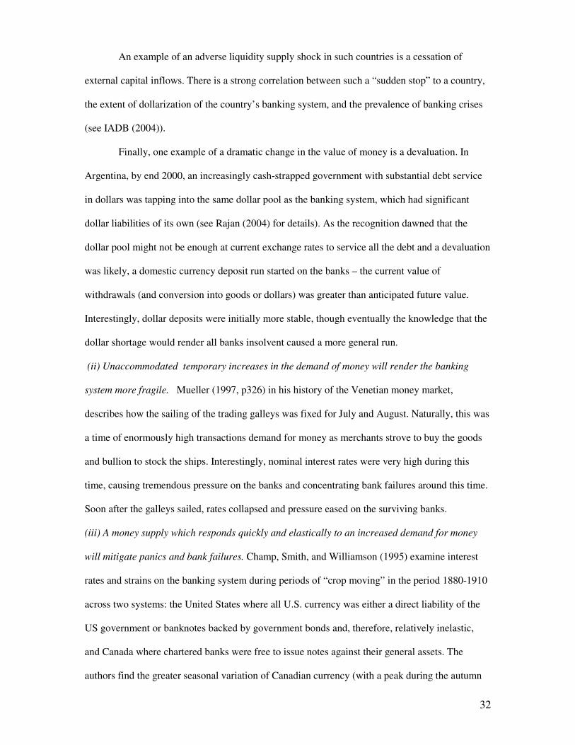
An example of an adverse liquidity supply shock in such countries is a cessation of

external capital inflows. There is a strong correlation between such a “sudden stop” to a country,

the extent of dollarization of the country’s banking system, and the prevalence of banking crises

(see IADB (2004)).

Finally, one example of a dramatic change in the value of money is a devaluation. In

Argentina, by end 2000, an increasingly cash-strapped government with substantial debt service

in dollars was tapping into the same dollar pool as the banking system, which had significant

dollar liabilities of its own (see Rajan (2004) for details). As the recognition dawned that the

dollar pool might not be enough at current exchange rates to service all the debt and a devaluation

was likely, a domestic currency deposit run started on the banks – the current value of

withdrawals (and conversion into goods or dollars) was greater than anticipated future value.

Interestingly, dollar deposits were initially more stable, though eventually the knowledge that the

dollar shortage would render all banks insolvent caused a more general run.

(ii) Unaccommodated temporary increases in the demand of money will render the banking

system more fragile. Mueller (1997, p326) in his history of the Venetian money market,

describes how the sailing of the trading galleys was fixed for July and August. Naturally, this was

a time of enormously high transactions demand for money as merchants strove to buy the goods

and bullion to stock the ships. Interestingly, nominal interest rates were very high during this

time, causing tremendous pressure on the banks and concentrating bank failures around this time.

Soon after the galleys sailed, rates collapsed and pressure eased on the surviving banks.

(iii) A money supply which responds quickly and elastically to an increased demand for money

will mitigate panics and bank failures. Champ, Smith, and Williamson (1995) examine interest

rates and strains on the banking system during periods of “crop moving” in the period 1880-1910

across two systems: the United States where all U.S. currency was either a direct liability of the

US government or banknotes backed by government bonds and, therefore, relatively inelastic,

and Canada where chartered banks were free to issue notes against their general assets. The

authors find the greater seasonal variation of Canadian currency (with a peak during the autumn

33

crop moving) was associated with much smoother interest rates. Currency fluctuated less in the

United States, resulting in greater fluctuations in interest rates, peaking around the crop moving

period. The banking panics of 1893 and 1907 in the United States indeed occurred during the

crop moving season.

(iv) Changes in monetary policy should most affect the lending decisions of the least liquid and

least creditworthy banks (lowα ). Kashyap and Stein (2000) find that the effect of monetary

policy on lending is indeed stronger for banks with less liquid balance sheets, that is, banks with

lower ratios of securities to assets. Moreover, this effect is primarily due to the smallest (and thus

least diversified) banks in their sample.

Other implications are less central. For instance, nominal deposits lend stability only if

the monetary authority can be relied upon to be appropriately state contingent. However, if they

do not have the necessary acumen or credibility, or have conflicting goals, nominal deposits are

destabilizing. This implies that countries with histories of weak monetary management are likely

to prefer real deposits (for example, through deposit dollarization) despite the attendant risks

because the alternative could be worse (also see Jeanne (2003)). De Nicolo, Honohan , and Ize

(2003) find that countries with weak institutions, high inflation, and high volatility of inflation

“dollarize” more, but have more financial depth (M2/GDP) than similar countries that do not.

5.2. Alternative Assumptions: Sticky Prices

The pattern of response of aggregate output to monetary expansion has been well studied

in the United States (see, for example, Bernanke and Gertler (1995)). One fact that is at odds with

our model is that prices do not adjust rapidly. While we think the fact that our model does not

require sticky prices to obtain monetary transmission is a virtue, we need to ask how we could get

transmission if prices were indeed sticky. It turns out that a simple extension is sufficient.

Consider a very simple search model where dealers first post prices at the beginning of

the period and buyers search for a seller. If the price cannot vary with supply or demand changes,

goods must be rationed. Assume the probability of a buyer meeting a dealer is an increasing

function of the ratio of supply of cash goods to demand at the posted price, P02. The nominal

34

supply of goods at date 0 is q1P02 and the nominal demand is the total amount of cash withdrawn

at date 0 by depositors. An open market operation that increases the amount of cash that can be

withdrawn by depositors will decrease the probability of each withdrawer finding a dealer. As

this probability decreases, the return from withdrawing cash falls toward the return of holding

cash to buy goods one period later, and the nominal interest rate on bank deposits between dates 0

and 1 will fall. The real payout burden on deposits at date 2 falls with an expansionary open

market operation, much as in the case of flexible prices. While sticky prices prevent the real price

level from changing immediately with changes in monetary policy, an immediate increase in the

supply of money will reduce the real value of withdrawing to make an immediate purchase.

5.3. Alternative Assumptions: Nominal Loans

We have discussed real loans thus far, with nominal or real deposits. This is consistent

with the assumption that resources are in short supply so the borrowing entrepreneur promises to

pay out the maximum possible ex ante by agreeing to an extremely high nominal repayment on

demand. As a result, actual repayments on project loans are renegotiated down to the underlying

real collateral value of assets. By contrast, bank deposits are enforced through the threat of

collective action, so their nominal face value matters, regardless of how high it is.

It is, however, interesting to discuss whether the system stabilizes automatically through

the price level if the nominal repayment on the project loan, L, were set at a level that did not

exceed the collateral value of underlying project assets (e.g., jkL CP< ). We have

PROPOSITION 5:

If the fiscal demand for money dominates and project loans are always nominal, then:

a) If deposits are also nominal, the representative bank will never fail at any α if it is solvent and

liquid at some 'α .

b) If deposits are real, the representative bank becomes (weakly) less solvent as α falls. Even if it

is solvent at an 'α , it can fail at some α < 'α .

Proof: See appendix.

35

When financial assets are all nominal and effectively have the same maturity, changes in

the price level have no effect on a bank’s nominal solvency, and cannot push a bank from

solvency to insolvency (or vice versa). However, price level changes will change the real value

of deposits and influence the real excess demand for liquidity. So long as there is a binding

liquidity constraint, policy induced increases in the price level will reduce the excess liquidity

demand, and will increase aggregate credit.

When loans are nominal but deposits are real, an increase in the price level reduces the

value of the bank’s assets without affecting liabilities. Since, ceteris paribus, a fall in the economy

wide fraction of early projects, α , (weakly) increases the price level, it can impair solvency.

Automatic changes in the price level do not stabilize the banking system when it has this kind of

asset-liability mismatch.

5.4. Alternative assumption: Capital.

For simplicity, banks in our model do not issue capital. Clearly, capital can buffer some

of the effects of liquidity shortages but it will also reduce the ability of the bank to commit to pay

depositors. An optimal capital structure will typically have the bank issuing a significant

proportion of its capital structure in deposits (see Diamond and Rajan (2000)) and, as we show in

the working paper version of this paper, liquidity shortages still are possible and all our results

continue to hold. The issuance of capital (or heterogeneity in project returns) will, however, result

in a much smoother and plausible path of real interest rates, 24r .

VI. Conclusion

Starting with the problem that banks are vulnerable to real liquidity shortages, we show

that they may be able to mitigate it by issuing nominal deposits. However, because bank deposits

can be converted on demand to money, this leaves them exposed to fluctuations in monetary

conditions. This suggests a “liquidity” channel of transmission of monetary policy, and a role for

monetary authorities in smoothing these conditions even in a world without many of the

traditional assumed frictions. Our model suggests why policy would work largely through banks.

36

There is ample scope for future work in expanding our simple model. For example, we

have only examined purchases with currency as the opportunity that causes strains on the banking

system. More generally, any opportunity that requires immediate nominal liquidity would strain

the system, and these deserve exploration. Also, our model ties the health of the banking system

to monetary and fiscal policies. We have only touched on monetary policy and not explored fiscal

policy (e.g., changes in the tax rate) at all. Also, we have made a number of strong assumptions to

simplify our analysis. The effect of relaxing some are easy to see. For example, initial investors

cannot substitute at all for consumption between dates. If they are willing to postpone

consumption once the interest rate rises enough, the destructive effects of liquidity shortages will

be capped. Similarly, allowing cash goods to be taxed will simply change the form of the fiscal

demand for money. But the effects of relaxing others are harder to anticipate. For instance, we do

not have long dated bonds nor do we incorporate concerns about monetary policy credibility or

fiscal performance. Relaxing each of these is a realistic and potentially interesting extension that

suggests scope for future work.

37

References

Allen, Franklin and Douglas Gale, [1998] “Optimal Financial Crises,” Journal of Finance 53, 1245 – 1284.

Bernanke, Ben, “Non-monetary effects of the financial crisis in the propagation of the Great

Depression”, The American Economic Review, Vol. 73, No. 3. (Jun., 1983), pp. 257-276. Bernanke, Ben S. ; Gertler, Mark, “Agency Costs, Net worth and Business Fluctuations”,

American Economic Review, Vol. 79, No. 1. (Mar., 1989), pp. 14-31. Bernanke, Ben S. ; Gertler, Mark, “Inside the Black Box: The Credit Channel of Monetary Policy

Transmission,” Journal of Economic Perspectives v9, n4 (Fall 1995): 27-48 Caballero, R, and A. Krishnamurthy [2000], “International Liquidity Management: Sterilization

Policy in Illiquid Financial Markets”, mimeo, MIT. Calomiris, Charles W. [1988], “Institutional Failure Monetary Scarcity and the Depreciation of

the Continental, Journal of Economic History 48 (March 1988): 47-68. Champ, Bruce, Bruce Smith, and Stephen Williamson, 1996. .Currency Elasticity and Banking

Panics: Theory and Evidence,. Canadian Journal of Economics 29, 828-864. Cochrane, John, “Money as Stock,” University of Chicago working paper, 2001, http://www-gsb.uchicago.edu/fac/john.cochrane/research/Papers/cashless2a.pdf Clower, R. [1967] “Reconsideration Of The Microfoundations Of Monetary Theory, Western

Economic Journal 6 (1): 1-8 1967 Diamond, Douglas W. [1997], “Liquidity Banks and Markets,” Journal of Political Economy,

105, 928-956. Diamond, D. W. and P. H. Dybvig [1983], .Bank Runs, Deposit Insurance, and Liquidity,.

Journal of Political Economy 91, 401-419. Diamond, Douglas W. and Raghuram Rajan A Theory of Bank Capital,. Journal of Finance 55

(December 2000): 2431-2465. Diamond, Douglas W. and Raghuram Rajan “Liquidity risk, liquidity creation and financial

fragility: A theory of banking,” Journal of Political Economy 109 (April 2001). Diamond, Douglas W. and Raghuram Rajan “Liquidity Shortages and Banking Crises,” Journal

of Finance (forthcoming, April 2005). Friedman, M and A. Schwartz [1963], A Monetary History of the United States 1867-1960.

Princeton: Princeton Univ Press. Gibson, Michael S. “More Evidence on the Link between Bank Health and Investment in Japan,”

Journal of the Japanese and International Economies v11, n3 (September 1997): 296-310. IADB (2004) Annual Report "Unlocking Credit: The Quest for Deep and Stable Bank Lending.",

forthcoming.

38

IMF 2004: “Debt Related Vulnerabilities and Financial Crises – An Application of the Balance Sheet Approach to Emerging Market Countries”, Mimeo.

Jeanne, Olivier, “Why do Countries borrow in a Foreign Currency?”, 2003, Working Paper, IMF. Kashyap, Anil K.; Stein, Jeremy C., “The Role of Banks in Monetary Policy: A Survey with

Implications for the European Monetary Union,” Federal Reserve Bank of Chicago Economic Perspectives v21, n5 (Sept.-Oct. 1997): 2-18.

Kashyap, Anil K.; Stein, Jeremy C. “The Impact of Monetary Policy on Bank Balance Sheets,”

Carnegie-Rochester Conference Series on Public Policy v42, n0 (June 1995): 151-95. Kashyap, Anil K.; Stein, Jeremy C. “What Do a Million Observations on Banks Say about the

Transmission of Monetary Policy?” American Economic Review v90, n3 (June 2000): 407-28.

Kashyap, Anil K.; Stein, Jeremy C. and Wilcox, David W., “Monetary Policy and Credit

Conditions: Evidence from the Composition of External Finance,” American Economic Review v83, n1 (March 1993): 78-98.

Lucas, Robert E. Jr., and Nancy L. Stokey, 1987, .Money and Interest in a Cash-in-Advance

Economy. Econometrica 55, 491-513. Ludvigson, Sydney C., “The Channel of Monetary Transmission to Demand: Evidence from the

Market for Automobile Credit.” Journal of Money, Credit, and Banking, August 1998, 30(3): 366-83.

Mueller, Reinhold, 1997, Money and Banking in Mediaeval and Renaissance Venice: Volume

II—The Venetian Money Market: Banks, Panics and the Public Debt 1200-1500, Johns Hopkins University Press, Baltimore and London.

Nicolo, G., Honohan, P., and A. Ize (2003), “Dollarization of the Banking System: Good or

Bad?”, IMF Working Paper 03/146. Rajan, Raghuram (2004), “Dollar Shortages and Crises”, mimeo, IMF. Romer, Christina D.; Romer, David H., “New Evidence on the Monetary Transmission

Mechanism,” Brookings Papers on Economic Activity v0, n1 (1990): 149-98. Skeie, David (2004) “ Money and Modern Bank Runs”, mimeo, Princeton University. Stein, J.C. (1998) “An adverse-selection model of bank asset and liability management with

implications for the transmission of monetary policy,”Rand Journal Of Economics 29 (3): 466-486.

Woodford, Michael, 1995, .Price Level Determinacy Without Control of a Monetary Aggregate,.

Carnegie-Rochester Conference Series on Public Policy 43, 1-46.

39

List of Symbols

C (After tax value of) goods produced by entrepreneur with project on maturity.

γ Fraction of entrepreneur’s production that can be produced by bank.

c (After tax value of) goods that can be produced by anyone if the project is

restructured.

jq Cash goods for sale on date j (j=1,3)

,G sθ Fraction of G type banks in state s. ,B sα Fraction of early projects in the portfolio of B type banks (for G banks, this is 1).

α Fraction of early projects in the portfolio of the representative bank. Bµ Fraction of late projects restructured by B banks (G banks have no late projects to

restructure).

µ Fraction of late projects restructured by the representative bank.

tX Total taxable goods produced on date t (t=2,4)

jd Face vale of real deposits due on date j

jδ Face vale of nominal deposits due on date j

jM Quantity of money available to make purchases on date j.

jB Face value of bonds (repaying in money) maturing on date j.

jkb Cash value on date j of bond maturing on date k.

jkr Real interest rate between date j and date k

jki Nominal interest rate between date j and date k

( )C

Rc

γ= Real interest rate necessary to give B banks an incentive to restructure late

projects

jkP The price in date i cash for a unit of date j consumption .

t Tax rate on produced goods

40

Figure 1: Time line of transactions:

Before Date 0 Banks offer interest rates on deposits and issues deposits for initial investors’ bonds and cash Entrepreneurs receive loans (in bank claims) Entrepreneurs buy goods from initial investors with bank claims Date 0 State realized Depositors withdraw cash to buy cash goods (if no more expensive than produced goods) or to hold as an asset. If a bank faces withdrawals exceeding its cash, it sells bonds and restructured loans for date-1 delivery to meet withdrawal (similarly on all future dates) Date 1 Cash goods sold at 0 delivered (similarly on all future dates) Cash from date 0 good sales available to seller to deposit or spend (similarly on all future dates) Cash from date 0 bank asset sales available for depositor to withdraw (similarly on all future dates) Early entrepreneurs sell produced goods for deposits or cash Date 2 Early entrepreneurs repay loans with deposits or cash Early entrepreneurs pay taxes with cash from sales and withdrawn bank deposits Government repays maturing bonds in currency and issues new bonds Cash is withdrawn to buy date-3 cash goods or to hold as an asset. Date 3 Cash goods sold at date 2 delivered Late entrepreneurs sell goods for bank claims and cash

Date 4 Late entrepreneurs repay bank with currency and deposits Banks repay remaining net deposits in currency Government repays maturing bonds in currency All currency goes to pay taxes

41

Appendix

Proof of Proposition 1:

We derived the price levels and interest rates after date 2 in the text. To determine the price level at dates prior to date 2, we have to determine the real value of all government liabilities at date 2. Since we already know the value of the money stock, we now determine the value of outstanding bonds.

Let the date-2 value in cash of bonds maturing to pay B4 at date 4 be b24. Then because of the competitive market for bonds,

4 224 4

24 23 3 2 4

4 4 4

3

24

2 4

{1, ( )}*1 }{1,

tX Mb B Min

q M BB B B

qi i Max M tXM B

= = =+

=

+

.

The real value (in date-4 consumption) of government liabilities leaving date 2 then is14: 4 2

2 424 3 2 4

24

3 4 4

2

24

4

2 4

{1, ( )}

.{ , }

tX MM B Min

q M BP

q tX tX

M bP

BMax

M B

+++ =

= ++

The quantity of money and bonds outstanding between date 0 to 2 are constant at 0M and 2B respectively (we will later allow monetary policy to alter these quantities). At date 2, the existing money stock and new money repaid on maturing date-2 bonds can be used to pay date-2 taxes as well as “buy” M2 and B4. The value of maturing bonds and money in units of date 2 consumption goods purchased at date 1 is

2 4 424

0 2 43

12 2 4

1 { , }tX tX tXr

M B BMax q

P M B+ = + +

+ (2.8)

where we use the real interest rate to transform units of date-4 consumption into units of date-2 consumption. At date 0, cash of M0 can be used to purchase cash goods q1 at date 1. So its real value in terms of date 2 consumption

10 0

02 12.{ , }q

M MMax

P P= (2.9)

Again, if 01

12

Mq

P> , money is valued for its transaction services and the nominal interest rate paid

by deposits and bonds from date 0 to 1 is 1 1

010 0 4

2 3 4 412 0 2 24 2 4

1[ { , ]

q qi

M M BtX Max q tX tX

P M B r M B

= =+ +

+ +

>1. The cash value of bonds at date 0

is 2 2

01 12 01*B B

i i i= .

14 We substitute for P24 and use 4 2 4 2

3 2 4 3 2 4

{1, ( )} ( )tX M tX M

Minq M B q M B

=+ +

and

23 4 3

2 4{ , }q tX q

MMaxM B

=+

when the nominal interest rate exceeds 1 to simplify the expressions.

42

In all of these expressions, the price level and the nominal interest rate depend on both the state of nature (through transaction demands,q1 and q3, output X2 and X4 and thus the fiscal demand, and the effect of liquidity conditions r24), and monetary policy variables (M0, M2, B2, B4).

Sketch that (2.3) is the market clearing condition

The claim follows because (i) deposits are also claims to bonds and money (which together are worth the value of taxes and cash goods), and (ii) goods are stored when there is excess supply. To see this, take the simple case where some late projects have to be restructured to meet aggregate liquidity demand, there are no cash goods, and aggregate bank assets just equal deposits. Since the real interest rate exceeds 1, there will be no storage. Now

0 2

12 242 (1 ) (1 ) (1 )(1 )G G B B B B BM B C

C C cP r

dγ

θ γ θ α γ µ α µ α+

+ + − + − + − −� �

= � �� �

. We know from

Proposition 1 that 0 2

12

M B

P

+=

24

(1 )(1 ) (1 )(1 )

1 (1 )

GG B B B BBC C

C crt t

θθ α µ α µ α

−+ + − + − −

� �� �− − � �

.

Substituting this in the expression for 2d and rearranging, we get

( )2 (1 ) (1 )1

1G G B B Bcd

tC Cθ θ α α µ+ − + −� �= � �−

24 24

) (1 ) ) (1 ) (1 )(1 (1 (1 )(1 ) (1 )(1 )(1 )

G G G GB B B B BCC t C

Cr t r

θ γ θ γ θ θγα µ α µ α− − − + − −− − − − + − −

−O

n the right hand side, the second term and third term are the (negative of) goods left with early entrepreneurs (of G and B banks respectively) after repaying their banks. The fourth term is the value deposited in the B bank and the last term is the value of future claims on the government

that are sold at date 2 ( 4 2 4

24 24 24

( )tX M Br r P

+= = ). For the early goods market to clear, the value of

future claims sold to early entrepreneurs should equal their holdings of early goods. So the terms on the second line of the right hand side sum to zero, leaving the condition on the first line that deposits should equal the pre-tax value of early goods produced, which is (2.3).

Proof of Proposition 2:

When there is no bank capital, the aggregate liquidity market clearing condition is:

( )1 21

(1 ) (1 )(1 )

G G B B BC C c d

tq θ θ α α µ+ − + − =

−+ � �� � .

This implies 2 1( )(1 ) ( (1 ))(1 )(1 )

G B GB

B G

d q t Cc

θ α θµα θ

− − − + −=

− −. As a result,

2 12

( )(1 )0

(1 )(1 )

B

G B G

C d q tc

µθ α θ

− − −∂ = − <∂ − −

and

2 12

( )(1 )0

(1 ) (1 )

B

B B G

C d q tc

µα α θ

− − −∂ = − <∂ − −

.

These are negative because 2 1( )(1 ) 0C d q t− − − > , which follows because if banks to avoid failure there must be sufficient liquidity to pay deposits in the best possible case, where all banks

43

are of type G (which requires that 1 21C

q dt

+ >−

). Of projects that are late, fewer are restructured

(more are continued, 1 Bµ− increases) when there is more aggregate liquidity. In addition more

aggregate liquidity increases the total credit (1 ){ (1 )(1 )}G G B B Bθ θ α α µ+ − + − − because it is

directly increasing in and G Bθ α , and 1 Bµ− is decreasing in them.

Finally,2

10

(1 )(1 )

B

B G

td cµ

α θ∂ −= >∂ − −

. An increase in real deposits requires increased

restructuring, this decreases total credit and the fraction of projects that are continued.

Proof of Proposition 4:

When net nominal interest rates are positive, we have the real payout on deposits at date

2, 0 12

0

qd

Mδ

= . Clearly, this falls as M0 increases. We showed in (2.33) in the proof of proposition 1

that a fall in d2 increases (1 )Bµ− , the amount of credit extended at date 2 by the B type banks,

or2

0Bd

ddµ > , and therefore

0 20

(1 )0

B

M B Const

ddM

µ+ =

− > .

Proof of Corollary 1 to Propostion 4.

First, some definitions. Total date 2 output of produced goods is

21

[ ] ( (1 )[ (1 ) ])1

B G G B B BX C C ct

µ θ θ α α µ= + − + −−

and on date 4 it

is 4[ ] (1 )(1 )(1 )1

B G B BCX

tµ θ α µ= − − −

−. Total date 2 liquidity is the sum of cash goods and

produced goods, 1 2[ ] [ ]B BL q Xµ µ= + . Let 0 'M and 2 'B be the quantity of money and bonds after the open market operations. We assume that the ratio of bond to money when refinancing

maturing debt at date 2, 4

2 4

BM B+

, is an constant, independent of changes in date 0 monetary

policy. The value of all nominal claims (money plus bonds) at date 2 is 4

2 24 2 3 4 424 2 4

1[ , ] [ ] { [ ], [ ]}B B B BB

N r tX Max q tX tXr M B

µ µ µ µ≡ + ++

and the date 2 present value of a

type B bank’s loans is 2424

[ , ] (1 ) (1 )(1 )B B B B B B Cr C c a

rγµ α γ µ α µΓ = + − + − − . The value of all of

a type B banks assets at date 2 is

' '' ' 0 2

2 24 0 2 2402 12

'2

1 2 24 2 24 24' '2 0

[ , , , ] [ , ]

{ [ , ], [ , ]} [ , ].

B B B

B B B

M BV r M B r

P P

BMax q N r N r r

B M

µ µ

µ µ µ

= + + Γ =

+ Γ+

+

For a type B bank to be solvent with no restructuring and for the goods market to clear:

' '0 1 2 240 2 1 2 24 0 2' ' '

02 0 0 2

[ 1, 0]max{ , } min{ [ 0] , [ 1, 0, , ]}

BB B Bq N r

X q V r M BP M M Bδ µδ µ µ= =

= ≤ = + = =+

.

For the goods market to clear with restructuring of (0,1]Bµ ∈ the condition is:

44

2 24' '0 1

0 2 1 2 24 0 2' ' '02 0 0 2

[ , ]max{ , } [ ] [ , , , ]}

B

B B B

CN rq Cc X q V r M B

P cM M B

γ µδ γδ µ µ=

= = + ≤ =+

. Depending on

which min and max is binding, there are several cases. Rather than detail all the cases, we sketch one:

Let 1 2 24[ , ]Bq N r µ≥ , then 1 2 24

0 0 2

[ , ]Bq N rM M B

µ>

+ for all 0 2 and M B , and the nominal interest rate

always exceeds one. Let ' '2 1 2 24 0 2[ ] [ , , , ]B B BX q V r M Bµ µ+ < .The money supply after open market

operations to keep the banking system solvent has to be ' 0 1 0 10 ' '

2 1 2 24 0 2 2 1min{ [ ] , [ , , , ]} [ ]B B B B

q qM

X q V r M B X qδ δ

µ µ µ≥ =

+ +. Let us determine if this can be

achieved with an open market operation. Given an open market operation at the market clearing

bond price from Proposition 1, of'

2 24 0' '

1 0 2

[ , ]( )

BN r Mq M B

µ+

, the quantities of money and bonds outstanding

adjust by ' ' ' ' '0 0 1 0 2 2 2 2 24 0( ) ( ) ( ) [ , ]BM M q M B B B N r Mµ− + = − . The feasibility of open market

operations then turns on whether there are enough bonds to buy back given the needed monetary

expansion. Solving for '2 ,B substituting ' 0 1

02 1[ ]B

qM

X qδµ

=+

, and then imposing the non-negativity

condition, we require 1 0 1 0 2 12

2 24 1 2

( ( [ ] )[ , ]( [ ])

B

B B

q q M X qB

N r q Xδ µ

µ µ− +

≥+

. If does not hold, open market operations

will repurchase bonds down to zero and additional helicopter drops of money will be necessary to ensure the banking system is solvent. Proof of Proposition 5:

(a) Suppose the nominal face value of a project loan is always L. This means that even when the project is late and the loan is restructured, the entrepreneur repays only L and keeps the residual of 02P c L− . Suppose also that the representative bank is solvent and liquid when α =1. Because it is solvent, L ≥ 2 0( )δ δ= . Then it is solvent at any otherα . To see this, note that for any

realizationα , the bank is solvent if 2

02 02 24 24 02

*(1 ) (1 )(1 )

L L L iP P r P P

δα α µ α µ+ − + − − ≥ , where i is the

nominal interest rate at which the project loan is rolled over for late projects. But the inequality holds if we set 1µ = because L ≥ 2δ . Since there is some µ at which the bank is solvent, and the banker can always choose it rather than be run, the bank will always be solvent. Since the liquidity condition does not depend on the actual repayment to the bank, the argument in footnote xx is valid even for nominal loans. So if the representative bank is solvent and liquid at some 'α , it is solvent and liquid at anyα . (b) Sketch: Since the number of late projects, the fraction restructured, and the real interest rate

24r all (weakly) increase as α falls, the price level 0 202 12

42

24

M BP P

Xt X

r

+= =

� �+� �

� �

will increase.

Now the solvency of the bank hinges on the rate i that loan repayments on late projects are rolled over at. Regardless of the precise bargaining process, a plausible assumption is that the value in date-2 consumption goods of the required payment on a continued loan does not increase as the value in date-2 consumption goods of a restructured loan falls. As α falls, not only are more

45

projects restructured but also the value in date-2 consumption goods of current nominal loan repayments of L will decrease because 02P increases (and hence, so (weakly) will the value in date-2 consumption goods of continued loans), as will the value of the financial assets on the bank’s balance sheet. Since the deposit repayments are fixed in real terms, the representative bank becomes weakly less solvent. The Financial Asset Channel of Transmission of Monetary Policy

Recall we showed that the real value of the claims on the government held by the banks is

2 4 424

0 2 43

12 2 4

1 { , }tX tX tXr

M B BMax q

P M B+ = + +

+ (2.10)

where B4 is the face value of date-4 maturing bonds issued at date 2 and M2 is the quantity of money left after date-4 maturing bonds are issued (=M0+B2-b24 where b24 is the present value of the date-4 maturing bonds issued at date 2). Keeping real activity constant, the expression indicates that as the quantity of bonds B4 that are issued decreases from a level that nearly absorbs the entire money stock (so that M2 is an infinitesimal amount) to 0, the total value of

government claims held by the banks decreases from 42

24

3 tXtX

rq ++ to 2 4

243

1 { , }tX tXr

Max q+ .

The decrease in the real value of government claims with expansionary open market operations is not because of seigniorage (government real revenues are assumed fixed): When there is only a minuscule amount of money outstanding, not only can current holders of money buy cash goods at a deeply discounted price, but also government bonds maturing at date 4 account for the lion’s share of the public’s claims on the government, so bonds capture the full value of real taxes. As the money stock increases, the dealers in the cash market at date 3 no longer have to sell goods for a deeply discounted price. Also bonds have to share the value of real taxes with holders of money. Therefore, as the amount of money outstanding increases relative to bonds, and as the nominal rate falls to 1, the real value of government liabilities (money plus bonds) holding real activity and real rates constant falls.15 Of course, once the nominal rate falls to one, no further alteration in value is possible, and further open market operations lose all effect.16

Thus expansionary open market operations reduce the real value of government assets held by banks at date 2, and reduce aggregate liquidity demand by reducing the real value of the bank’s liabilities. This leads to an expansion in bank credit for similar reasons to the ones discussed in the previous sub-section. The “financial asset” channel is probably weaker than the “liquidity” channel because the former works primarily by altering the value of bank liabilities such as capital that are most sensitive to bank asset values (unlike the latter which works by altering the real value of deposit payouts). In practice, non-deposit bank liabilities are less likely to be held for liquidity or transactions purposes, and thus the change in their value will have less of an effect on the aggregate demand for liquidity.

15 Contrast this with the effect on nominal liabilities. Pushing down the nominal interest rate increases the nominal value of bonds and the total nominal value of government claims. 16 Note also that the government’s real revenues are unchanged if real output does not change (and government expenditure is fixed). So substituting interest-bearing liabilities for non-interest bearing ones does not result in a greater real claim on the government or in lower seigniorage profits. There are no sticky prices in our model. Open market operations simply transfer value from one set of agents to others but do not alter the aggregate real future payments by the government.