Embed Size (px)
Citation preview
NBER WORKING PAPER SERIES
‘OPTIMAL’ POLLUTION ABATEMENT -WHOSE BENEFITS MATTER, AND HOW MUCH?
Wayne B. GrayRonald J. Shadbegian
Working Paper 9125http://www.nber.org/papers/w9125
NATIONAL BUREAU OF ECONOMIC RESEARCH1050 Massachusetts Avenue
Cambridge, MA 02138September 2002
Financial support for the research from the National Science Foundation (grant # SBR-9410059) and theEnvironmental Protection Agency (grant # R-828824-01-0) is gratefully acknowledged. We are also gratefulto the many people in the paper industry who have been willing to share their knowledge with us. ThomasMcMullen, Charles Griffith, George Van Houtven, and Tim Bondelid helped us work with the EPA datasets;thanks to Mahesh Podar and John Powers in the EPA Office of Water, sponsors of the NWPCAM model. Wereceived helpful comments on earlier drafts of the paper from Eli Berman, Matt Kahn, Arik Levinson, GilbertMetcalf, and seminar participants at the EPA’s National Center for Environmental Economics, the PublicChoice Meetings, the Second World Congress of Environmental and Resource Economists, and the NBEREmpirical Environmental Policy Research Conference. Capable research assistance was provided byAleksandra Simic, Martha Grotpeter, and Bhramar Dey. Any remaining errors or omissions are the authors’.The views expressed herein are those of the authors and not necessarily those of EPA, NSF or the NationalBureau of Economic Research.
© 2002 by Wayne B. Gray and Ronald J. Shadbegian. All rights reserved. Short sections of text, not toexceed two paragraphs, may be quoted without explicit permission provided that full credit, including ©notice, is given to the source.

‘Optimal’ Pollution Abatement – Whose Benefits Matter, and How Much?Wayne B. Gray and Ronald J. ShadbegianNBER Working Paper No. 9125September 2002JEL No. Q28, L51
ABSTRACT
We examine measures of environmental regulatory activity (inspections and enforcement
actions) and levels of air and water pollution at approximately 300 U.S. pulp and paper mills, using data
for 1985-1997. We find that levels of air and water pollution emissions are affected both by the benefits
from pollution abatement and by the characteristics of the people exposed to the pollution. The results
suggest substantial differences in the weights assigned to different types of people: the benefits received
by out-of-state people seem to count only half as much as benefits received in-state, although their
weight increases if the bordering state’s Congressional delegation is strongly pro-environment. Some
variables are also associated with greater regulatory activity being directed towards the plant, but those
results are less consistent with our hypotheses than the pollution emissions results. One set of results
was consistently contrary to expectations: plants with more nonwhites nearby emit less pollution. Some
of our results might be due to endogenous sorting of people based on pollution levels, but an attempt
to examine this using the local population turnover rate found evidence of sorting for only one of four
pollutants.
Wayne B. Gray Ronald J. ShadbegianEconomics Department Economics DepartmentClark University University of Massachusetts, Dartmouth950 Main Street 285 Old Westport RoadWorcester, MA 01610 Pittsburgh, PA 15260and NBER and U.S. EPA, [email protected] [email protected]
1
‘Optimal’ Pollution Abatement – Whose Benefits Matter, and How Much?
1. INTRODUCTION
In this paper we examine the optimal allocation of environmental regulation across pulp
and paper mills. The optimal allocation depends on the costs and benefits of pollution abatement
at the plant, as seen by the regulator. The direct costs of pollution abatement at a particular plant
are related to the plant’s age, size, and technology, while the benefits are related to the extent of
the pollution being generated and the number of people affected. Past studies comparing
benefits and costs have focused on fairly simple measures of abatement benefits. In this study
we develop more sophisticated measures of air and water benefits from pollution abatement
based on the SLIM-3 Air Dispersion Model and the Environmental Protection Agency’s (EPA)
National Water Pollution Control Assessment Model (NWPCAM) respectively. We expect that
regulators should impose stricter regulation on plants located in areas with greater benefits from
pollution abatement. However, we also consider political factors that may influence the
allocation of pollution abatement. The focus of our paper is on spatial differences across plants
in the distribution of benefits from pollution abatement and in the characteristics of the
population living nearby. Responding to some of these population measures may be socially
optimal if certain population groups are more sensitive to pollution, but in many cases these
measures suggest self-interested behavior by regulators seeking to maximize the political support
for their actions.
We perform our analyses using a plant-level panel data set on approximately 300 pulp
and paper mills from 1985-1997. We find substantial supporting evidence for both benefits and

2
population characteristics affecting environmental outcomes. Plants with larger benefits to the
overall population emit less air and water pollution, and those with more kids and elders nearby
emit less air pollution. Plants located in poor neighborhoods get less regulatory attention and
emit more pollution. Plants located near state boundaries emit more pollution, with these effects
reduced if the nearby states have more pro-environment Congressmen. Not every result fits
those predicted by theory: the percentage nonwhite near the plant, expected to reduce regulatory
attention (assuming nonwhites have less political clout), is actually associated with lower
emissions. The results for our measures of regulatory activity tend to be less often significant,
and sometimes carry unexpected signs.
One important caveat on our results is the cross-sectional nature of our demographic data.
Some of the results could be explained as reverse causation or sorting: poor people move
towards dirty neighborhoods because housing is cheaper there; families with sensitive
individuals such as kids and elders avoid dirty neighborhoods. It is difficult for us to control for
such endogeneity because most paper mills are very old, so we cannot include pre-siting
demographics in the analysis. Our attempt to test for sorting (using the degree of population
turnover near the plant) finds significant evidence in favor of sorting for only one of the four
pollutants (particulates), while the two water pollutants find significant evidence against sorting.
Some of the differences in results for different regulatory measures pose further research
questions. There is a pattern of unexpected signs for regulatory actions, where factors associated
with fewer regulatory actions are often associated with less, not more, pollution. We would have
expected opposite signs on these coefficients, and do find opposite signs in some cases. Is this
an artifact of the data, or does it represent a real difference in the process by which regulatory

3
activity is allocated in different situations? Similarly, we find different effects on air and water
pollution of being near the Canadian border: do these reflect real differences across pollution
media in the mechanisms for ensuring international cooperation on pollution control?
The remainder of the paper is organized as follows. Section 2 provides a brief survey of
the relevant literature. In section 3 we provide some background on the pulp and paper industry.
Section 4 outlines our model of the regulator’s allocation of pollution abatement across plants.
In section 5 we present our empirical methodology and a description of our data. Section 6
contains our results and finally we present some concluding remarks and possible extensions in
section 7.
2. PREVIOUS STUDIES
A few studies have addressed the issues raised above, providing empirical estimates of
the impact of political boundaries, demographics, and political activism on exposure to pollution.
For example, Helland and Whitford (2001), using annual county-level data from the Toxic
Release Inventory (1987-1996), find that facilities located in counties on state borders (border
counties) have systematically higher air and water pollution releases than facilities located in
non-border counties: facilities in border counties emit 18 percent more air pollution and 10
percent more water pollution than facilities in non-border counties. Kahn (1999) also finds some
evidence of a transboundary externality problem with particulates. Kreisel et al (1996) find that
minorities are not disproportionately exposed to TRI emissions, but find some evidence that the
poor are disproportionately exposed to TRI emissions. Arora and Cason (1999) find evidence of
racial injustice only in the south. In particular, Arora and Cason find that race is a significantly
positive determinant of TRI releases in non-urban areas of the south.

4
Hamilton (1993, 1995) examines whether exposure to environmental risk varies by
demographics and political activism. Using data at the ‘zip-code neighborhood level,’ he relates
the capacity expansion/contraction decisions of commercial hazardous waste facilities to race,
income, education, and level of political activity (voter turnout), finding that capacity expansions
are negatively correlated with voter turnout. Jenkins, Maguire, and Morgan (2002) show that
minority communities receive lower ‘host’ fees for the siting of land fills while richer
communities receive higher ‘host’ fees. Wolverton (2002) examines the issue of the location
decision of ‘polluting’ plants. Previous studies indicate that ‘polluting’ plants tend to locate in
poor and minority neighborhoods. However, Wolverton shows that once you consider the
characteristics of the community at the time the plant is sited that contrary to popular opinion
race no longer matters and that poor neighborhoods actually attract disproportionately less
‘polluting’ plants.1
3. PULP AND PAPER INDUSTRY BACKGROUND
During the past 30 years environmental regulation has increased considerably both in
terms of stringency and levels of enforcement. In the late 1960s environmental rules were
primarily enacted at the state level, and were not vigorously enforced. Since the creation of the
Environmental Protection Agency (EPA) in the early 1970’s the federal government has been the
lead player in proposing and developing stricter regulations, and in encouraging greater
emphasis on enforcement (much of which is still performed by state agencies, following federal
guidelines). The expansion in environmental regulation has imposed large costs on traditional
1 Been (1994) and Been and Gupta (1997) find mixed results for environmental injustice in the citing of hazardous waste facilities when considering the characteristics of the neighborhood at the time of citing – however, their results are based on data sets with only 4 and 10 observations respectively.

5
‘smokestack’ industries, like the pulp and paper industry, which is one of the most impacted
industries due to its sizable generation of both air and water pollution.
The pulp and paper industry as a whole faces a high degree of environmental regulation.
However, plants within the industry can face very different impacts from regulation, depending
in part on the technology being used (pulp and integrated mills vs. non-integrated mills2), the
plant's age, the plant’s location, and the level of regulatory effort directed at the plant. The most
important determinant of the regulatory impact is whether or not the plant contains a pulping
process. Pulp mills begin with raw wood (chips or entire trees) and use a variety of techniques
to separate out the wood fibers, which are then used to produce paper. The most common form
of pulping in the U.S. is the Kraft technique, which separates the wood into fibers using
chemicals. A large number of plants also use mechanical pulping (giant grinders separating out
the fibers), while still others use some combination of heat, other chemicals, and mechanical
methods. Once the fibers are separated out, they can be bleached and combined with water to
produce a slurry. After the pulping stage is complete, residual matter remains which historically
was released directly into rivers (hence water pollution), but now must first be treated. The
pulping process is energy intensive, so most pulp mills have their own power plant, and thus are
significant sources of air pollution. The pulping processes may also involve hazardous
chemicals, such as the use of chlorine bleaching in Kraft pulp mills, which can create trace
amounts of dioxin, raising the concern over toxic releases.
The paper-making process is not nearly as pollution intensive as pulping. Non-integrated
mills either purchase pulp from other mills or use recycled wastepaper. During the paper-
making process, the slurry (more than 90% water at the beginning) is laid on a rapidly-moving
2 Integrated mills produce their own pulp and non-integrated mills purchase pulp or use recycled wastepaper.

6
wire mesh which progresses through a succession of dryers in order to remove the water, thereby
creating a continuous sheet of paper. The energy required during this stage is less than during
the pulping stage, but it can still cause air pollution concerns if the mill produces its own power.
Finally, during the drying process some residual water pollution is created. However, both of
these pollution concerns are much smaller than those created during the pulping process.
The past 30 years has seen large reductions in pollution from the paper industry, with the
advent of secondary wastewater treatment, electrostatic precipitators, and scrubbers. In addition
to these end-of-pipe control technologies, some mills have altered their production process, more
closely monitoring material flows to lower emissions. Overall these alterations have been much
more prevalent at newer plants, which were at least partly designed with pollution controls in
mind – some old pulp mills were deliberately built on top of the river, so that any spills or leaks
could flow through holes in the floor for ‘easy disposal.’ These rigidities can be partially or
completely offset by the tendency for most regulations to include grandfather clauses exempting
existing plants from the most stringent requirements – e.g. until recent standards limiting NOx
emissions, most small existing boilers were exempt from air pollution regulations.
4. MODEL OF POLLUTION ABATEMENT REGULATION
Why do profit-maximizing plants employ resources to abate pollution emissions? If
pollution were a pure externality, with all the burden falling on those who live downwind or
downstream, we would not expect to see any profit-maximizing plant spend money on pollution
abatement. Some market-based mechanisms like consumer demand for ‘green’ products or
managerial taste for ‘good citizenship’ may provide incentives for plants to abate pollution.
However, we believe that the main motivation for controlling pollution emissions in the U.S. is

7
government regulation of pollution, especially for the air and water pollutants being considered
in this paper, so we model the amount of pollution abatement as being determined by regulators
rather than by the polluting firms. One could instead employ other models, in which pressure
from regulators is supplemented by pressure from customers and community groups, or in which
the polluting firms are concerned about some groups of people but not others, affecting where
pollution levels are greater. These alternative models could lead to analyses similar to those
presented here (explaining why pollution levels from paper mills differ depending on which
groups of people are affected by the pollution). We are also assuming that differences in
regulatory pressures among U.S. paper mills are primarily determined at the state level, so we
view the state as the relevant jurisdiction for political concerns.
A socially optimal government regulator maximizes social welfare by increasing the
stringency of environmental regulation (requiring greater pollution abatement) up to the point
where the marginal benefit from another unit of abatement is equal to the marginal cost of that
abatement. In equation (1), the regulator would choose different optimal abatement values Ai*
for each plant, based on differences in factors affecting their marginal benefits and marginal
costs of abatement. The marginal costs of abatement differ across plants based on their
production technology, size, and age. The marginal benefits of abatement also differ across
plants, driven especially by the number (and characteristics) of the people near the plant who are
being exposed to the pollution. Assuming that the marginal cost of pollution abatement
increases with stringency (or at least cuts the marginal benefit curve from below), an increase in
the marginal benefits curve (or decrease in the marginal costs curve) results in an increase in the
desired level of pollution abatement and more stringent environmental regulation. Therefore
dAi*/dPLANTi<0 for PLANT characteristics that raise marginal costs, and dAi*/dPEOPLEi>0

8
for PEOPLE characteristics that raise marginal benefits.
Our analysis focuses on the differences across plants in the marginal benefits of pollution
abatement (MBi), though we do include plant characteristics affecting abatement costs as control
variables. We model the regulator as adding up the marginal benefits from pollution reductions
for all people living around a plant, as shown in equation (2) below. The locations of the people
are indexed by x and y. The marginal benefits MBi for pollution reductions at a given plant will
depend heavily on the number of people in the area (measured by ρxy, the population density at a
given point) and the emissions that they are exposed to (Exy). People may also differ in their
susceptibility to pollution exposure (Sxy), which should affect MBi. The ‘base’ Sxy value would
be 1, with deviations from this affecting MBi. Finally, the regulator may choose αxy to value
certain people less than others when calculating benefits (in which case αxy would be less than 1).
Why would αxy differ across people affected by pollution? One strand of the literature
raises concerns with “Environmental Justice”, suggesting that groups with less political
influence (e.g. the poor or minorities) are discriminated against by regulatory agencies (i.e. are
assigned a smaller value of αxy) which aim at maximizing political clout. Politically active
people who strongly favor environmental issues might put more pressure on regulators, and
hence get a larger value of αxy. For plants located near a state (or country) boundary, the benefits
dxdyxy
ρESα MBi)( xyxyxyxy∫∫=2
*)A ,MB(PEOPLE *)A ,(PLANT MC (1) iiii =

9
from pollution reduction may accrue to people in other jurisdictions for whom αxy might be
expected to be zero (or at least less than one). However, some countervailing pressures may
arise to offset the latter transboundary effect on regulatory activity.
The creation of a federal EPA in 1972 was at least in part designed to limit cross-state
pollution flows, and EPA oversight of state regulatory decisions may be stricter for plants near
state boundaries. In addition to a dummy for a plant being located near the border with another
state, we include a measure of the pro-environment stance of the neighboring state’s
Congressional delegation, since presumably the airing of the neighboring state’s objections to
any transboundary pollution is likely to occur in a national setting.
In the case of Canada two agreements exist which are designed to limit the levels of
transboundary pollution: 1) Canada-United States Great Lakes Water Quality Agreement
(GLWQA) of 1972 and 2) Canada-United States Air Quality Agreement (AQA) of 1991.3 The
GLWQA establishes that the U.S. and Canada will act to restore and preserve the chemical,
physical and biological soundness of the Great Lakes Basin Ecosystem and it contains a number
of goals and guidelines to reach those goals. The AQA is the first bilateral pact between the U.S.
and Canada aimed at controlling transboundary air pollution caused by sulfur dioxide and
nitrogen oxide emissions.4 Given these two agreements it is possible that plants along the
Canadian border will face more stringent (or at least no less stringent) environmental regulation.
3 A memorandum of intent has been in place since 1981. 4 For more information on both of these agreements see the web site (http://www.ijc.org/ijcweb-e.html) of the International Joint Commission which was created by the International Boundary Waters Treaty Act of 1909.

10
5. DATA AND EMPIRICAL METHODOLOGY
Our study measures the relationship between regulatory activity and emissions, and
characteristics of the surrounding population, using data on the intensity of environmental
regulation faced by U.S. pulp and paper mills. We use data on both air and water pollution, to
measure the enforcement and monitoring activity directed towards each mill, along with the
relative stringency of the pollution limits faced by the mill. To measure actual outcomes from
regulation at the mill we use data on both air and water pollution emissions at the mill. Our
analysis controls for a variety of plant- and firm-specific characteristics, as well as the past
compliance status of the mill. We also include a number of other control variables designed to
capture characteristics of the location of the mill that could influence the level of regulatory
activity.
We use models of the spread of pollution to estimate the relative impacts of the pollution
on people living near the plant. On the air pollution side, the model utilizes an air dispersion
model, SLIM-3, which calculates the total impacts of pollution on the surrounding population
separately at each plant. The air dispersion model incorporates information from the pollution
source (stack height and characteristics of the pollutants being emitted) and meteorological data
(mixing height, wind directions and speeds) to calculate the aggregate exposure at all points
within a wide circle around the plant. The exposure data is combined with measures of the
number of people living near the plant and estimates from the literature on the health impact of
pollutant exposures to quantify the overall dollar benefits from reducing air pollution at each
plant [see Shadbegian et al. (2000) for more details].
On the water pollution side we use data from the EPA’s National Water Pollution Control
Assessment Model (NWPCAM). This model includes discharge data for over 50,000 industrial

11
and 13,000 municipal water polluters, combined with stream and river flow data to calculate the
transport of pollutants downstream and the resulting water quality on a mile-by-mile basis for
every affected stream. Of the paper mills in our dataset, 231 have data present in the NWPCAM
model. For each of these mills, we first calculate a baseline model using current discharges and
store the water quality results. We then estimate 5 scenario models, increasing the pollution
discharged from the mill by a wide range of amounts, and measuring how each scenario affects
water quality downstream of the plant. Our monetary measures of the benefits of pollution
abatement are based on an experimental version of the NWPCAM model being developed for
EPA at Research Triangle Institute, which uses a continuous water quality index (0-100) rather
than the traditional four-valued outcomes (unusuable, boatable, fishable, swimmable), allowing
for a more precise valuation of water quality changes. Changes in water quality in each stream
mile are evaluated in dollar terms using a formula based on the work of Carson and Mitchell
(1993). These dollar values are then combined with state population and river miles to estimate
the total dollar benefits of pollution reduction (in terms of improved usability) for each scenario.
These costs are divided by the amount of additional pollution being discharged in that scenario,
providing us with a per-unit benefit of pollution reduction. The largest per-unit value from the 5
scenarios is used to estimate the marginal benefits of pollution abatement at that mill.
Detailed data on the characteristics of the population within a 50-mile radius of each
plant, including age distribution, racial composition, and within-jurisdiction residency, are based
on the 1990 U.S. Census of Population, as compiled in the Census-CD datasets prepared by
Geolytics, Inc. This provides information based on detailed geographic areas (block groups).
Distances are calculated between the paper mill and the centroid of each block group to
determine which block groups fall within 50 miles of the mill, and the block group values for

12
each population characteristic are aggregated to get the overall value for each mill.
In past studies we developed a comprehensive database of U.S. pulp and paper mills to
study the impact of environmental regulation on plant-level productivity and investment. This
database includes published plant-level data from the Lockwood Directory and other industry
sources to identify each plant's production, investment, productivity, age, production technology,
and corporate ownership. We add financial data taken from Compustat, identifying firm
profitability.
Our pulp and paper mill data is merged with annual plant-level information on regulatory
enforcement, compliance, and quantities of pollution, for both air and water pollution, taken
from EPA regulatory databases. Regulatory enforcement and compliance data for 1985-1997
come from the EPA’s Envirofacts and Integrated Data for Enforcement Analysis databases, as do
the water pollution discharges data for Biochemical Oxygen Demand (BOD) and Total
Suspended Solids (TSS). These datasets allow us to differentiate between two different types of
regulatory actions – enforcement actions (e.g. notice of violation) and inspections. Based on
conversations with regulators, the number of enforcement actions is more likely to be connected
with problems at the plant, while the number of inspections is more connected with the plant’s
size. Air pollution emissions data for particulates (PM10) and sulfur dioxide (SO2) comes from
the Aerometric Information Retrieval System database for 1985-1990 and from the National
Emissions Inventory for 1990-1997.
Our analyses consider two different measures of the environmental regulatory pressures
faced by each plant. The number of inspections and the number of enforcement actions received
by the plant provide direct measures of regulatory attention. The level of air pollution emissions
and water pollution discharges from the plant provide an indirect measure of the regulatory

13
pressures faced by the plant, all else equal (assuming that other variables included in the
analyses control for differences in the amount of pollution from the plant in the absence of
regulation).
Each dependent variable Yit is a function of PLANT and PEOPLE characteristics, as
well as STATE variables and year dummies:
where Y is one of the eight dependent variables in our analysis: Air and Water Pollution
Inspections and Enforcement, Water Discharges of BOD and TSS, and Air Emissions of PM10
and SO2. Since increased regulatory activity will be seen (directly) in more inspections and
enforcement actions, and (indirectly) in less air and water pollution, we expect to find opposite
signs for the coefficients in the regulatory activity and pollution quantity equations.
First, let us review the plant-, firm-, state-, and county-level control variables included in
each model. These controls include lagged compliance status, plant capacity, plant age, firm
financial condition, county attainment status (air only), major source and public health effects
(water only), and state environmental attitudes. All the results presented here include state
dummies, but the models without state dummies tend to lead to similar conclusions (results
available from authors upon request). To avoid having the state dummies absorb too much of the
cross-plant variation, we only include state dummies for states with 5 or more plants in the given
regression (e.g. the air pollution inspection model includes 22 state dummies, with the base
group being all other non-specified states).
In terms of plant-level controls we include a lagged measure of regulatory compliance
(COMPLAG). Previous research has shown a strong relationship between compliance and
enforcement [Magat and Viscusi (1990); Deily and Gray (1991); Nadeau (1997); and Gray and
)YEAR ,STATE ,PEOPLE ,f(PLANT Y )3( titititit =

14
Shadbegian (2000)]. We also include pulp and paper capacity (PULP/PAPER CAPACITY) to
control for plant size, a dummy variable to indicate if the plant was established after 1960 (NEW
PLANT), and a dummy variable to indicate if the plant is the only paper or pulp mill owned by
the firm (SINGLE). We also include the number of the plant’s Occupational Safety and Health
Agency’s violations (OSHA VIOL), since previous research has shown that OSHA violations
are positively correlated with EPA violations [see Gray and Shadbegian (2000)]. To indicate the
financial health of the plant we include a measure from Compustat of the owning-firm’s rate of
return on its assets (RETURN ON ASSETS).
We include three additional variables to control for exogenous factors affecting the level
of regulatory stringency faced by the plant. On the air side we include a dummy variable to
indicate if the plant is located in a county that is in non-attainment status with respect to
particulate standards (NONTSP; in our data non-attainment for sulfur dioxide is much less
common, and nearly always overlaps with particulate non-attainment, so we focus on
particulates for all equations). On the water side we include a numeric rating from EPA’s
Majors Rating Database indicating the extent to which the plant is a large water polluter
(MAJORS) and a dummy variable to indicate if the plant discharges into a stream whose water
quality has potential health effects, due to being a source of drinking water (PUBLIC HEALTH).
We control for the state-level regulatory climate using GREEN VOTE, a measure of
support for environmental legislation by that state’s Congressional delegation. The League of
Conservation Voters calculates a scorecard for each member of Congress on environmental
issues, with data available back to the early 1970s. We use the average score for the state's
House of Representative members in our analysis. We also measured the overall inspection
activity in each state for each year by the total number of inspections in the state divided by the

15
number of plants in the EPA database for that state (STATE AIR INSPECTIONS and STATE
WATER INSPECTIONS). The unemployment rate in the state for that year (UNEMP) and
percent of the county designated as urbanized (URBAN) round out our control variables.
Now consider the variables which are at the heart of our analyses, those influencing the
marginal benefits from pollution abatement at a particular mill (MBi in equation 2). As
described above, we have information on the expected benefits per unit of pollution reduction
(AIRBEN and WATBEN). On the air pollution side, we also have the percentage of the nearby
population under the age of 6 (KIDS) and those 65 and over (ELDERS) representing groups with
greater sensitivity to air pollution (Sxy in equation 1). We would expect each of them to be
positively related to regulatory activity (inspections and enforcement actions), and negatively
associated with pollution quantities.
Differences in αxy across people are measured with several variables. We test for
Environmental Justice factors by including two measures of potentially “less valued”
populations: poor and minorities. POOR is the percentage of the nearby population living below
the poverty line. The minority variable is the percentage of the population that is nonwhite
(NONWHITE). We would expect both to be negatively associated with regulatory activity and
positively associated with pollution levels.
A positive influence on αxy is expected to come from voter activity, measured using voter
turnout in the previous presidential election (TURNOUT), which should be positively associated
with regulatory activity. This sort of voter activity to overcome externalities is discussed in
Olson (1965). However, it is possible that in some cases a majority of the electorate could
oppose environmental regulation, so that higher turnout need not always increase regulation.
Thus we include an interaction between turnout and state membership in conservation

16
organizations (TURNOUT*CONVMEMB), which would be expected to have a positive
association with regulatory activity.
We test for the effects of political boundaries by including two simple dummy variables
indicating whether the plant is within 50 miles of another jurisdiction (STATE BORDER or
CANADIAN BORDER). For these plants, some of their pollution may “spill over” to the other
jurisdiction. All else equal, regulators should care less about such pollution, so regulatory
activity should be diminished for those plants. However, the other jurisdiction(s) could respond
strongly to any transboundary pollution. Depending on the institutional arrangements in place,
the political costs associated with transboundary pollution could be larger than the costs of
intrastate pollution. For cross-state pollution, the sensitivity of the other state to transboundary
pollution (and hence the pressure to reduce such pollution) is presumed to be associated with that
state’s GREEN VOTE measure of pro-environmental Congressional support.
An alternative approach to these benefit-related variables is to disaggregate the total
benefits received by the surrounding population into those received by different groups, in an
effort to see whether the coefficient on benefits differs across groups. To our regressions we add
an interaction between the total benefits and the share of the surrounding population in each
group, so that the coefficients on the interaction terms show the differences across groups. To
measure transboundary effects on the air pollution side we assume that the benefits are
distributed proportionately to the fraction of the population within 50 miles of the plant that is
out-of-state. On the water pollution side we measure the benefits for each out-of-state river
segment directly (where a river forms the border between states, half of the benefit is allocated to
each state).
We estimate the eight different equations for the dependent variables measuring
17
regulatory stringency using two statistical techniques. For both air and water pollution we
measure stringency as the number of inspections (INSP) and enforcement actions (ENFORCE) a
plant receives in a given year. Since both INSP and ENFORCE are often zero and are otherwise
relatively small integers, we estimate the equations using a Poisson model (actually, we use a
Negative Binomial model, to allow for the observed over-dispersion of the data, relative to the
simpler Poisson model). For the four pollution quantity equations, we use ordinary least squares
on the logarithm of emissions quantities because of the wide dispersion in emissions across
plants.
6. RESULTS
Table 1 contains the means and standard deviations (along with variable descriptions) of
all variables used in this study. Note that the number of observations varies across the models
being estimated, depending on the availability of data for the dependent variable and some
specific explanatory variables. We have more data for regulatory activity (inspections and
enforcement actions) than we do for pollution quantities. To avoid having too many different
sample sizes, we restrict the pollution quantity estimation to plants which have both pollutants
reported. To simplify Table 1, all of the control variables have their values reported only for the
largest dataset, corresponding to air pollution regulatory activity.
In our data the average plant-year observation receives nearly ten times as many
inspections as enforcement actions: approximately two air or water pollution inspections per
year and one air or water enforcement action every three or more years. The distribution of
enforcement actions is skewed in our data, with many plants receiving none and others receiving
several. There is also substantial variation across plants in their air emissions and water
18
discharges.
Considering the control variables, the marginal benefits from pollution abatement vary
substantially for both air and water pollution. There is much less variation in the age-related
demographics variables (KIDS and ELDERS) compared to the ‘environmental justice’ variables
(POOR and NONWHITE). Most plants are within 50 miles of a state border, while a sizable
fraction are near the Canadian border. Most plants are in compliance with air and water
regulations (84% and 70% compliance rates respectively). Most plants were in existence by
1960 (75%) and are owned by a firm with more than one paper mill (75%). Approximately half
of the plants (43%) have water pollution discharges that have potential public health impacts and
34% of the plants are located in counties that are not in attainment with particulate emission
standards.
Tables 2 and 3 present the results of the basic model for air pollution and water pollution
regulation respectively. Consider first the control variables in each equation. We see that lagged
compliance is associated with significant reductions in both pollution quantities and regulatory
activity for air pollution, but for water pollution the only marginally significant impact comes in
reduced water inspections. OSHA violations are surprisingly associated with lower pollution
quantities (though significant only for SO2), and more enforcement actions. The effects of plant
capacity seem to come primarily in terms of pulping capacity, rather than paper capacity (larger
coefficients and more frequently significant). Larger plants generate more pollution and face
more regulatory activity (except water inspections). Plants in urban areas generate less
pollution, but also (surprisingly) face somewhat less regulatory activity. Plants in areas with
high unemployment rates generate more air pollution and less water pollution, and face more air
enforcement actions. The time trends are mostly unremarkable. The base year is 1985 (during

19
the Reagan administration) except for the water pollution quantity equations which use a base
year of 1989 (during the Bush administration). We see significantly higher regulatory activity
and lower pollution quantities during the Clinton administration (except for water inspections,
which are significantly lower).
Now consider the benefits-related variables that are the focus of our analysis. The
marginal benefits per unit of pollution abatement for the overall population are associated with
lower pollution levels (significant for all pollutants except for sulfur dioxide), but are
surprisingly associated with significantly less air regulatory activity. The sensitive population
groups (KIDS and ELDERS) are significantly negatively related to air pollution quantities, but
also fewer air regulatory actions. Since the dependent variables are measured in log form, the
coefficients reflect percentage impacts on pollution. For example, a one standard deviation
increase in ELDERS (.019) is associated with 27 percent lower SO2 pollution and 19 percent
lower particulate pollution; the comparable reductions for KIDS (.006) are 27 percent and 10
percent. On the air side, a one standard deviation increase in pollution abatement benefits (1.3 in
logs) is associated with 18 percent lower particulate emissions and 20 percent lower sulfur
dioxide emissions. On the water side, the results (for a 2.0 increase in log benefits) show 11
percent lower BOD and 14 percent lower TSS.
The results for the “Environmental Justice” variables are mixed. POOR has the expected
effects in most cases: significantly more air and water pollution, and fewer enforcement actions
(although unexpectedly more inspections). However, the NONWHITE coefficient is always
opposite in sign from POOR, and usually significant. It appears that nonwhites are not being
discriminated against by regulators, although the poor may be.
Plants which are located in areas of high political activity and high support for

20
environmental regulation, as measured by TURNOUT*CONVMEMB, are expected to face more
regulatory activity and have less pollution. Pollution levels are significantly lower as expected,
although the greater relative magnitude of the TURNOUT coefficient for the water pollution
models means that the net effect of greater TURNOUT is more pollution for all but relatively
high CONVMEMB states. The regulatory activity results are unexpected, as states with high
turnout and above-average CONVMEMB values are associated with less, rather than more,
regulatory activity for all but air enforcement actions.
The border effects in Tables 2 and 3 do not follow the expected pattern. Plants which are
located near state borders show no significant differences in water pollution and lower
particulate pollution, and there is more air pollution where the bordering states are stronger
environmentally.5 The results for Canadian plants suggest different impacts for different
pollutants. On the water pollution side we observe more BOD pollution and less regulatory
activity. On the air pollution side we observe less SO2 pollution and more enforcement actions.
This discrepancy across pollution media suggests that it might be valuable to examine the
mechanisms for regulatory cooperation between the US and Canada more closely.
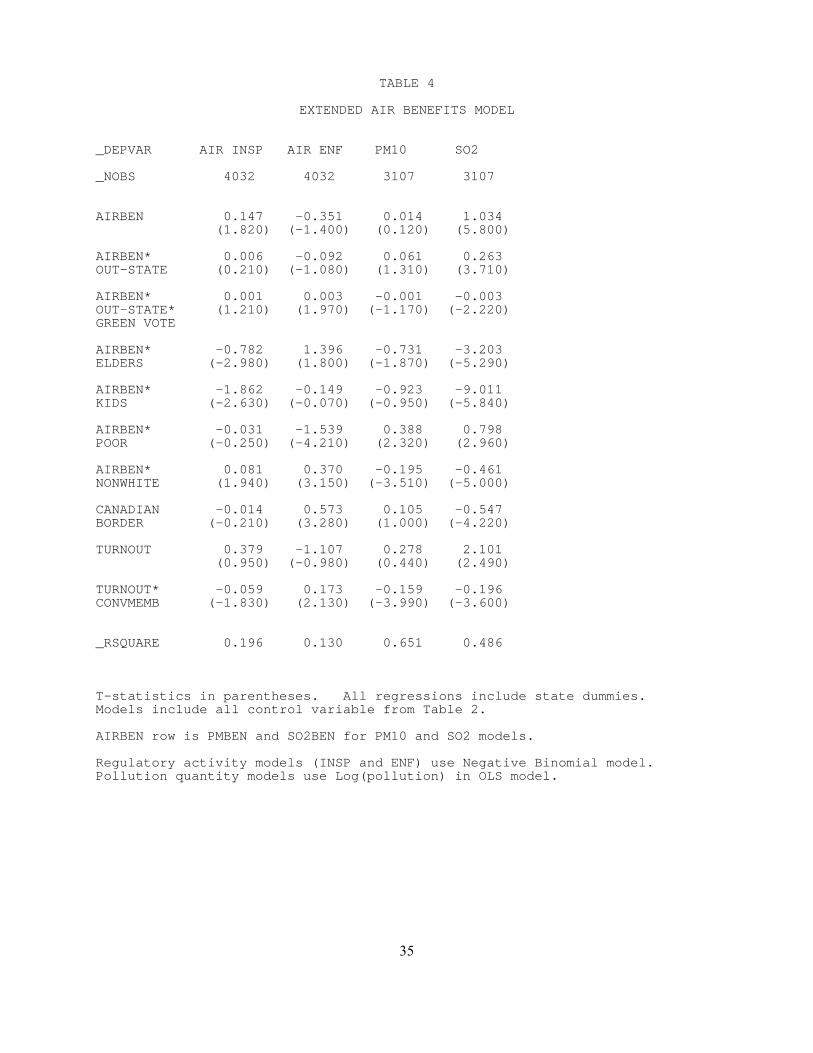
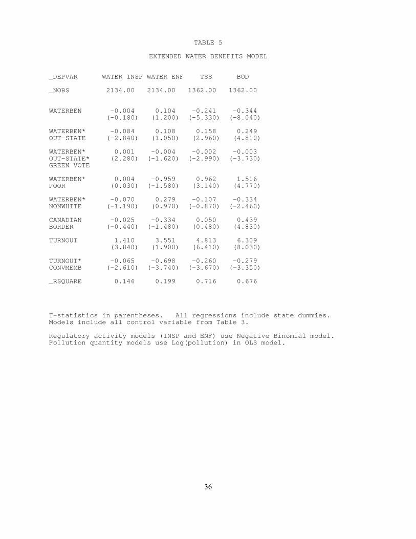
Tables 4 and 5 present the results when the various population characteristics are
interacted with the benefits from pollution abatement, to test for differences across groups in the
‘weight’ given their benefits when determining regulatory stringency. These results are similar
to those in Tables 2 and 3 for the different population characteristics. We see greater benefits
being associated with lower pollution levels at plants with low values of POOR and high values
of KIDS, ELDERS and (surprisingly) NONWHITE. Because of the large negative effects of the
5 This is due at least in part to the use of 50 mile circles to define being near a state border - most of our plants are near a state border by this definition. Earlier analyses using a 5 mile circle to define state borders find significantly greater pollution at border plants, and lower pollution when those border states are stronger environmentally.

21
interactions with KIDS and ELDERS the non-interacted AIRBEN coefficient becomes positive,
but when we evaluate the overall AIRBEN effect at the mean values of the various interactions
we still get a negative impact of -0.14 on particulates and –0.15 on sulfur dioxide. The
comparable numbers for WATBEN are –0.13 for TSS and –0.19 for BOD.
More importantly, we now get the expected results for the state border variables. Plants
near other states have more pollution, but this effect is reduced when the neighboring state is
stronger environmentally. How large are these effects? Recall that the overall impact of
AIRBEN on sulfur dioxide was –0.15. The AIRBENOUT coefficient of 0.263 combined with
the AIRBENOUT*VOTE coefficient of –0.003 evaluated at the mean GREENVOTE of 54
reduces this effect to –0.05, indicating that benefits outside the state have only one-third the
impact of within-state benefits. Changes in the neighboring state’s GREENVOTE from one
standard deviation below average to one standard deviation above average (from 36 to 72)
change this effect from +0.005 to –0.10, a shift of about two-thirds of the in-state benefits. The
impacts for other pollutants are similar, with benefits to people in high-GREENVOTE border
states having nearly as great an impact as people in the plant’s own state, while people in low-
GREENVOTE border states count substantially less (except for particulates, where the
interaction term is small). As before, the regulatory activity equations are less consistent with
the model, with more air regulatory activity being faced by plants with benefits outside the state.
The Canadian border effects are similar to those in the earlier models.
We can also try to quantify the impact of changes in demographics around a plant using
the coefficients in Tables 4 and 5. For sulfur dioxide, a one standard deviation increase in
ELDERS increases the impact of benefits by about one-third, from -0.15 to -0.21 (for KIDS it
increases the impact to -0.20); a comparable increase in POOR reduces the impact of benefits by
22
about one-quarter, to –0.11. There is some variation in impact across pollutants, less on
particulates and more on water pollutants, but overall the results show substantial impacts of the
demographics around a plant on the responsiveness of our environmental measures to the
marginal benefits of abatement.
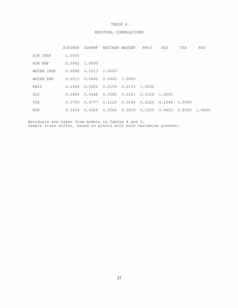
Given that each model is being estimated for eight different equations (four air and water
pollutants, along with inspections and enforcement equations), one might wonder whether the
unobserved factors influencing each equation are correlated. To test this, we calculated the
residuals for each of the 8 equations in Tables 4 and 5, and checked the correlations among these
equations. The results are presented in Table 6. The only large correlations come for pollutants,
where plants with surprisingly high emissions of one pollutant also tend to emit surprisingly
large amounts of the other pollutant in that same media. These values are quite high, with
correlations of about 0.8 between BOD and TSS discharges and 0.55 between particulates and
sulfur dioxide emissions. Correlations between air and water pollutants are on the order of .1 to
.2, and correlations among the different measures of regulatory activity tend to be .1 or less.
One issue for interpreting our results is the possibility that certain population
characteristics may be endogenous – driven by people sorting themselves between locations
based on the pollution in those areas, rather than the pollution levels at plants being driven by
regulatory pressures which depend on the population characteristics. Wolverton (2002) deals
with the sorting issue by examining a set of plants that are relatively young, and including
population characteristics from before the plants began operations. Unfortunately for our
analysis, most paper mills are quite old (only 25% of our plants started operations after 1960,
and very few started after 1980). In any event, population data at a detailed geographic level for
non-urban areas are first available in the 1990 Census of Population, and that’s what we use
23
here.
Tables 7 and 8 present the results from an alternative analysis, focusing on the results for
the POOR variable. The poor are arguably the ones most likely to have their location decisions
driven by pollution characteristics, if greater pollution reduces housing values and attracts more
poor residents. Suppose that areas around plants differed in terms of the mobility of the
population, for reasons other than pollution levels. In the areas where the population moves
more often there will be more opportunity for endogenous sorting to occur. SORTING is the
fraction of the population near the plant in 1990 which had moved there since 1985. We interact
SORTING with POOR, and expect to see positive coefficients on POOR*SORTING in the
pollution level equations if sorting matters. We do find a significant positive coefficient for one
of the four pollution equations (particulates), but significant negative coefficients for both of the
water pollution results (and insignificant positive results for SO2). These results suggest that the
positive POOR coefficients found for all four pollutants in the earlier tables are not primarily due
to bias caused by endogenous sorting.
7. CONCLUSIONS AND POSSIBLE EXTENSIONS
In this paper we use a plant-level panel data set on approximately 300 pulp and paper
mills from 1985-1997 to examine the allocation of environmental regulation across plants. We
focus on the benefit side of the MB=MC equation, and find that plants in areas with higher
marginal benefits of pollution abatement have lower pollution levels. Demographics also matter,
as plants with more kids, more elders, and fewer poor people nearby emit less pollution. Plants
near state boundaries emit more pollution, with these boundary effects reduced if the bordering
states have more pro-environment Congressional delegations. Plants in areas with politically

24
active populations that are also environmentally conscious emit less pollution.
Not every result fits the predictions of our model. The percentage nonwhite near the
plant, expected to reduce regulatory attention in the Environmental Justice model, is actually
associated with more regulatory activity and lower emissions. The results for the regulatory
activity equations are generally less consistent with our hypotheses than those for the emissions
equations. Perhaps regulators use other, unmeasured, mechanisms to control emissions levels,
such as the details of the air and water permit requirements for each plant. Still, the significant
results for the air pollution emissions and water pollution discharges suggest an important role
for these benefit-side factors in determining the environmental regulation faced by different
plants.
One important caveat on the results is the cross-sectional nature of our demographic data.
Some of our results could be explained as reverse causation or sorting: poor people move
towards dirty neighborhoods because housing is cheaper there; families with sensitive
individuals such as kids and elders avoid dirty neighborhoods. It is difficult for us to control for
such endogeneity because most paper mills are very old, so we cannot include pre-siting
demographics in the analysis. Our attempt to test for sorting (using the degree of population
turnover near the plant) finds significant evidence in favor of sorting for only one of the four
pollutants (particulates), while the two water pollutants find significant evidence against sorting.
On the positive side, some of the differences in results for different regulatory measures
pose further research questions. There is a pattern of unexpected signs for regulatory activity,
where factors associated with less regulatory activity are often associated with less pollution,
when we expected opposite signs on these coefficients. Is this an artifact of the data, or does it

25
represent a real difference in the process by which regulatory activity is allocated in different
situations? Similarly, do the different effects on air and water pollution of being near the
Canadian border reflect real differences across pollution media in the mechanisms for ensuring
international cooperation on pollution control?
Potential extensions of this project include a more detailed examination of these border
effects and the differences between air and water pollution regulation. We plan to distinguish
between state and federal enforcement and to explore other ways to more accurately measure the
political activism of a community. We will test whether a plant’s pollution abatement spending
is also affected by the benefits of pollution abatement. Finally, we will examine the results for
other industries, to see whether our results for the paper industry hold up in other settings.

26
REFERENCES
S. Arora and T. N.Cason, “Do Community Characteristics Influence Environmental Outcomes? Evidence from the Toxic Release Inventory”, Southern Economic Journal 65, 691-716 (1999). V. Been, “Locally Undesirable Land Uses in Minority Neighborhoods: Disproportionate Siting or Market Dynamics,” The Yale Law Journal 103, 1383-1421 (1994). V. Been and F. Gupta, “Coming to a Nuisance or Going to a Barrios? A Longitudinal Analysis of Environmental Justice Claims,” Ecology Law Quaterly 24, 1-56 (1997). R.T. Carson and R.C. Mitchell, “The Value of Clean Water: The Public’s Willingness to Pay for Boatable, Fishable, and Swimmable Quality Water,” Water Resources Research 29, 2445-2454 (1993). Council of State Governments, “Resource Guide to State Environmental Management,” Lexington, Kentucky (1991). M. E. Deily and W. B. Gray, Enforcement of Pollution Regulations in a Declining Industry, Journal of Environmental Economics and Management 21, 260-274 (1991).
W. B. Gray and R. J. Shadbegian, “When is Enforcement Effective -- or Even Necessary?, presented at the Association of Environmental and Natural Resource Economists (June 2000), NBER Summer Institute (August 2000). W. B. Gray and R. J. Shadbegian, “What Determines the Environmental Performance of Paper Mills? The Roles of Abatement Spending, Regulation, and Efficiency,” presented at the American Economic Association Meetings (January 2001) and the Western Economic Association Meetings (July 2001). R. Hall and M. L. Kerr, “Green Index: A State-by-State Guide to the Nation’s Environmental Health,” Island Press, Washington, D.C. (1991). J. Hamilton, Politics and Social Costs: Estimating the Impact of Collective Action on Hazardous Waste Facilities, Rand Journal of Economics 24, 101-125 (1993). J. Hamilton, Testing for Environmental Racism: Prejudice, Profits, Political Power?, Journal of Policy Analysis and Management 14, 107-132 (1995). E. Helland and A. B. Whiford, “Pollution Incidence and Political Jurisdiction: Evidence from the TRI,” presented at the American Economic Association Meetings (January 2001) and the Western Economic Association Meetings (July 2001).

27
REFERENCES (cont.) R. Jenkins, K. Maguire and C. Morgan, “Host Community Compensation and Municipal Solid Waste Landfills,” U.S. Environmental Protection Agency, National Center for Environmental Economics mimeo (2002). M. E. Kahn, The Silver Lining of Rust Belt Manufacturing Decline, Journal of Urban Economics 46, pp. 360-376 (1999). W. Kreisel, T. J. Centner, and A. G. Keeler, Neighborhood Exposure to Toxic Releases: Are Their Racial Inequities?, Growth and Change 27. 479-499 (1996). W. A. Magat and W. K. Viscusi, Effectiveness of the EPA's Regulatory Enforcement: The Case of Industrial Effluent Standards, Journal of Law and Economics 33, 331-360 (1990). L. W. Nadeau, EPA Effectiveness at Reducing the Duration of Plant-Level Noncompliance, Journal of Environmental Economics and Management 34, 54-78 (1997). Mancur Olson, “The Logic of Collective Action,” Harvard University Press, Cambridge, MA (1965). R. J. Shadbegian, W. B. Gray, and J. Levy, “Spatial Efficiency of Pollution Abatement Expenditures,” presented Harvard University's Kennedy School of Government's Lecture Series on Environmental Economics (March 2000) and at NBER Environmental Economics session (April 2000). A. Wolverton, “Race Does Not Matter: An Examination of a Polluting Plant’s Location Decision,” U.S. Environmental Protection Agency, National Center for Environmental Economics mimeo (2002).

28
TABLE 1
DESCRIPTIVE STATISTICS(N=4032, air enforcement dataset, unless otherwise noted)
VARIABLE (N) MEAN (STD DEV) {log mean,std}
Dependent Variables
AIR INSP 2.396 (4.214)Number of air pollution inspections
AIR ENF 0.356 (1.143)Number of air pollution enforcement actions
PM10 (N=3107) 369.2 (608.7) {4.32,2.18}Tons of particulate emissions per year
SO2 (N=3107) 1722.7 (3232.7) {5.83,2.42}Tons of sulfur dioxide emissions per year
WATER INSP (N=3431) 1.650 (1.560)Number of water pollution inspections
WATER ENF (N=3431) 0.183 (0.710)Number of water pollution enforcement actions
BOD (N=2113) 4061 (8258) {7.20,1.75}Biological oxygen demand discharged
TSS (N=2113) 7611 (31442) {7.48,1.93}Total suspended solids discharged
Key Explanatory Variables
AIRBEN 2997 (4092) {7.27,1.30}Marginal benefit of air pollution abatement (particulate + SO2) ($1990/ton)
PMBEN 3528 (4834) {7.44,1.29}Marginal benefit of particulate air pollution abatement ($1990/ton)
SO2BEN 1431 (1907) {6.56,1.27}Marginal benefit of SO2 air pollution abatement ($1990/ton)
WATERBEN (N=3431) 327.2 (834.1) {3.37,1.86}Marginal benefit of water pollution abatement (BOD + TSS)($1990/unit)
KIDS 0.087 (0.006)Percentage of the population under 6 years old
ELDERS 0.131 (0.019)Percentage of the population 65 years old and over
POOR 0.135 (0.051)Percentage of the population living below the poverty line

29
Table 1 (cont.)
NONWHITE 0.137 (0.132)Percentage of the population who are nonwhite
TURNOUT 41.673 (6.859)Percentage of the population over 18 voting in previous presidential election
STATE BORDER PLANT 0.655 (0.476)Dummy indicating a plant located within 50 miles of a state border
CANADIAN BORDER PLANT 0.126 (0.332)Dummy indicating a plant located within 50 miles of the Canadian border
Control Variables
AIR COMPLAG 0.835 (0.371)Dummy variable indicating (lagged) compliance with air pollution regulations
WATER COMPLAG (N=3431) 0.703 (0.457)Dummy variable indicating (lagged) compliance with water pollution regulations
PULP CAPACITY 404.1 (630.4) (2.893,3.284)Plant capacity - tons of pulp per day
PAPER CAPACITY 497.7 (582.5) (4.999,2.266)Plant capacity - tons of paper per day
NEW PLANT 0.249 (0.433)Dummy variable indicating the plant was opened after 1960
SINGLE 0.247 (0.431)Dummy variable indicating that this is the only paper plant owned by the firm
MAJOR SOURCE (N=3431) 114.627 (37.388)Numeric majors rating from the EPA’s Majors Rating Database
PUBLIC HEALTH (N=3431) 0.430 (0.495)Dummy variable indicating the potential public health impact of discharges
RETURN ON ASSETS 0.023 (0.056)Rate of return on assets (Compustat)
OSHA VIOL 0.293 (0.408)Fraction of OSHA inspections with violations (3-year moving average, last-this-next years)
STATE AIR INSPECTIONS 0.294 (0.160)Overall air pollution inspection rate in state (inspections/plants)
STATE WATER INSPECTIONS 0.527 (0.289)Overall water pollution inspection rate in state (inspections/plants)
NONTSP 0.342 (0.474)Dummy indicating plant is located in non-attainment area for TSP

30
Table 1 (cont.)
URBAN 39.140 (39.22)Percent of county designated as urbanized
GREEN VOTE 54.309 (17.768)Pro-environment Congressional voting (League of Conservation Voters)
UNEMP 6.000 (1.584)State unemployment rate
CONVMEMB 8.957 (3.386)Membership in 3 conservation groups, late 1980s, per 1000 population

31
TABLE 2BASIC AIR MODEL
_DEPVAR AIR INSP AIR ENF PM10 SO2
_NOBS 4032 4032 3107 3107
AIRBEN -0.101 -0.313 -0.169 -0.060(-3.360) (-3.780) (-4.120) (-1.200)
ELDERS -4.091 8.643 -9.945 -14.028(-2.300) (1.720) (-3.750) (-3.940)
KIDS -11.646 -0.747 -16.710 -45.774(-2.260) (-0.050) (-2.430) (-4.770)
POOR -0.506 -10.456 2.426 5.002(-0.570) (-4.340) (2.040) (2.920)
NONWHITE 0.557 2.712 -1.136 -3.184(1.670) (3.230) (-2.720) (-5.170)
STATE -0.098 -0.589 -0.452 -0.087BORDER (-0.990) (-1.910) (-3.090) (-0.420)
STATE BORDER 0.003 0.013 0.008 0.005*GREEN VOTE (1.840) (2.380) (3.190) (1.540)
CANADIAN 0.004 0.542 0.093 -0.533BORDER (0.060) (2.990) (0.860) (-3.940)
TURNOUT 0.169 -1.279 0.737 1.512(0.420) (-1.160) (1.190) (1.750)
TURNOUT* -0.053 0.193 -0.217 -0.227CONVMEMB (-1.690) (2.420) (-5.700) (-4.300)
Control Variables
AIR COMPLAG -0.323 -0.943 -0.583 -0.849(-6.880) (-8.680) (-7.340) (-8.640)
PULP 0.117 0.199 0.348 0.307CAPACITY (15.500) (9.130) (25.380) (17.760)
PAPER -0.009 -0.031 -0.026 0.033CAPACITY (-1.020) (-1.370) (-2.060) (2.010)
NEW PLANT -0.046 0.172 0.243 0.140(-1.140) (1.590) (3.990) (1.620)
SINGLE -0.089 -0.236 -0.249 -0.083(-2.050) (-1.830) (-3.810) (-0.920)
RETURN ON 0.562 -0.185 1.679 1.809ASSSETS (2.120) (-0.220) (1.850) (1.620)
OSHA -0.003 0.597 0.004 -0.271VIOL (-0.060) (3.610) (0.050) (-2.430)
STATE AIR 2.150 -0.029 -0.039 -0.079INSPECTIONS (19.790) (-0.230) (-0.510) (-0.810)

32
TABLE 2BASIC AIR MODEL (cont.)
_DEPVAR AIR INSP AIR ENF PM10 SO2
NONTSP 0.037 -0.029 -0.039 -0.079(0.830) (-0.230) (-0.510) (-0.810)
URBAN -0.001 0.002 -0.002 -0.005(-2.320) (1.260) (-2.980) (-4.460)
GREEN VOTE 0.000 -0.015 -0.007 0.003(0.130) (-2.640) (-2.290) (0.770)
UNEMP 0.011 0.181 0.039 0.085(0.700) (3.410) (1.730) (2.840)
YR86 0.168 1.199 -0.007 0.010(2.100) (3.060) (-0.050) (0.060)
YR87 0.125 1.700 -0.044 -0.012(1.570) (4.640) (-0.310) (-0.070)
YR88 0.178 2.012 -0.086 0.049(1.980) (5.330) (-0.600) (0.280)
YR89 0.075 2.254 -0.052 0.016(0.860) (5.900) (-0.370) (0.090)
YR90 0.156 2.012 -0.263 -0.191(1.840) (5.430) (-1.910) (-1.130)
YR91 0.070 1.603 -0.436 -0.298(0.860) (4.380) (-3.390) (-1.830)
YR92 0.262 1.624 -0.396 -0.382(3.120) (4.500) (-2.980) (-2.230)
YR93 0.258 2.194 -0.314 -0.514(3.090) (6.150) (-2.450) (-3.070)
YR94 0.247 2.575 -0.284 -0.425(2.860) (7.250) (-2.230) (-2.530)
YR95 0.202 2.288 -0.341 -0.451(2.240) (6.170) (-2.540) (-2.520)
YR96 0.100 2.461 -0.622 -0.620(1.090) (6.500) (-4.440) (-3.480)
YR97 0.131 2.905 -0.553 -0.621(1.270) (7.730) (-3.920) (-3.400)
_RSQUARE 0.196 0.130 0.653 0.481
T-statistics in parentheses. All regressions include state dummies.
AIRBEN row is PMBEN and SO2BEN for PM10 and SO2 models.
Regulatory activity models (INSP and ENF) use Negative Binomial model.Pollution quantity models use Log(pollution) in OLS model.

33
TABLE 3BASIC WATER MODEL
_DEPVAR WATER INSP WATER ENF TSS BOD
_NOBS 3431 3431 2113 2113
WATERBEN 0.003 0.036 -0.076 -0.123(0.370) (1.060) (-5.080) (-8.610)
POOR 1.538 -1.915 5.258 6.287(2.790) (-0.840) (4.300) (5.340)
NONWHITE -1.048 1.862 -3.866 -3.516(-3.550) (1.880) (-6.230) (-5.870)
STATE -0.014 -0.162 0.122 0.061BORDER (-0.170) (-0.520) (0.830) (0.420)
STATE BORDER -0.001 0.003 0.000 0.001*GREEN VOTE (-0.390) (0.590) (0.000) (0.270)
CANADIAN -0.079 -0.192 0.061 0.431BORDER (-1.510) (-1.050) (0.570) (4.430)
TURNOUT 1.324 2.332 3.294 4.686(3.990) (1.420) (4.620) (6.700)
TURNOUT* -0.071 -0.308 -0.313 -0.354CONVMEMB (-2.850) (-1.880) (-4.870) (-5.410)
Control Variables
WATER COMPLAG -0.054 -0.018 -0.021 0.004(-1.800) (-0.120) (-0.330) (0.070)
MAJORS 0.004 0.004 0.014 0.012(9.850) (2.130) (9.680) (8.960)
PUBLIC 0.074 0.218 -0.003 0.081HEALTH (2.190) (1.630) (-0.040) (1.080)
PULP -0.010 0.053 0.219 0.186CAPACITY (-1.650) (2.050) (17.000) (14.120)
PAPER 0.001 0.013 -0.049 -0.050CAPACITY (0.200) (0.390) (-3.970) (-4.340)
NEW PLANT -0.014 -0.327 0.102 0.029(-0.440) (-2.130) (1.550) (0.440)
SINGLE 0.010 0.412 -0.222 0.047(0.260) (2.660) (-2.790) (0.600)
RETURN ON -0.061 1.210 -0.306 -0.307ASSETS (-0.400) (0.960) (-1.140) (-1.560)
OSHA -0.016 0.321 -0.130 -0.109VIOL (-0.370) (1.720) (-1.510) (-1.330)
STATE WATER 1.730 0.237 -0.318 -0.259INSPECTIONS (13.810) (0.440) (-1.470) (-1.190)

34
TABLE 3BASIC WATER MODEL (cont.)
_DEPVAR WATER INSP WATER ENF TSS BOD
URBAN -0.000 -0.004 -0.002 -0.002(-0.200) (-2.150) (-2.080) (-1.790)
GREEN VOTE 0.000 0.005 -0.004 -0.002(0.180) (0.620) (-0.970) (-0.430)
UNEMP -0.004 0.025 -0.137 -0.155(-0.340) (0.450) (-3.390) (-3.910)
YR86 -0.019 0.495(-0.290) (1.070)
YR87 -0.186 0.890(-2.760) (2.160)
YR88 -0.033 1.154(-0.480) (2.660)
YR89 -0.065 1.202(-0.920) (2.900)
YR90 -0.133 1.184 0.065 0.078(-1.950) (2.930) (0.560) (0.710)
YR91 -0.165 1.494 0.162 0.182(-2.510) (3.740) (1.190) (1.340)
YR92 -0.309 1.484 0.039 0.096(-4.530) (3.560) (0.260) (0.680)
YR93 -0.381 0.804 0.018 -0.017(-5.600) (2.040) (0.140) (-0.140)
YR94 -0.312 1.207 -0.101 -0.168(-4.640) (3.020) (-0.790) (-1.380)
YR95 -0.338 0.970 -0.236 -0.282(-4.590) (2.300) (-1.820) (-2.210)
YR96 -0.399 0.736 -0.279 -0.307(-5.240) (1.730) (-2.190) (-2.420)
YR97 -0.469 0.649 -0.358 -0.392(-6.160) (1.430) (-2.800) (-3.040)
_RSQUARE 0.123 0.164 0.622 0.578
T-statistics in parentheses. All regressions include state dummies.
Regulatory activity models (INSP and ENF) use Negative Binomial model.Pollution quantity models use Log(pollution) in OLS model.
35
TABLE 4
EXTENDED AIR BENEFITS MODEL
_DEPVAR AIR INSP AIR ENF PM10 SO2
_NOBS 4032 4032 3107 3107
AIRBEN 0.147 -0.351 0.014 1.034(1.820) (-1.400) (0.120) (5.800)
AIRBEN* 0.006 -0.092 0.061 0.263OUT-STATE (0.210) (-1.080) (1.310) (3.710)
AIRBEN* 0.001 0.003 -0.001 -0.003OUT-STATE* (1.210) (1.970) (-1.170) (-2.220)GREEN VOTE
AIRBEN* -0.782 1.396 -0.731 -3.203ELDERS (-2.980) (1.800) (-1.870) (-5.290)
AIRBEN* -1.862 -0.149 -0.923 -9.011KIDS (-2.630) (-0.070) (-0.950) (-5.840)
AIRBEN* -0.031 -1.539 0.388 0.798POOR (-0.250) (-4.210) (2.320) (2.960)
AIRBEN* 0.081 0.370 -0.195 -0.461NONWHITE (1.940) (3.150) (-3.510) (-5.000)
CANADIAN -0.014 0.573 0.105 -0.547BORDER (-0.210) (3.280) (1.000) (-4.220)
TURNOUT 0.379 -1.107 0.278 2.101(0.950) (-0.980) (0.440) (2.490)
TURNOUT* -0.059 0.173 -0.159 -0.196CONVMEMB (-1.830) (2.130) (-3.990) (-3.600)
_RSQUARE 0.196 0.130 0.651 0.486
T-statistics in parentheses. All regressions include state dummies.Models include all control variable from Table 2.
AIRBEN row is PMBEN and SO2BEN for PM10 and SO2 models.
Regulatory activity models (INSP and ENF) use Negative Binomial model.Pollution quantity models use Log(pollution) in OLS model.
36
TABLE 5
EXTENDED WATER BENEFITS MODEL
_DEPVAR WATER INSP WATER ENF TSS BOD
_NOBS 2134.00 2134.00 1362.00 1362.00
WATERBEN -0.004 0.104 -0.241 -0.344(-0.180) (1.200) (-5.330) (-8.040)
WATERBEN* -0.084 0.108 0.158 0.249OUT-STATE (-2.840) (1.050) (2.960) (4.810)
WATERBEN* 0.001 -0.004 -0.002 -0.003OUT-STATE* (2.280) (-1.620) (-2.990) (-3.730)GREEN VOTE
WATERBEN* 0.004 -0.959 0.962 1.516POOR (0.030) (-1.580) (3.140) (4.770)
WATERBEN* -0.070 0.279 -0.107 -0.334NONWHITE (-1.190) (0.970) (-0.870) (-2.460)
CANADIAN -0.025 -0.334 0.050 0.439BORDER (-0.440) (-1.480) (0.480) (4.830)
TURNOUT 1.410 3.551 4.813 6.309(3.840) (1.900) (6.410) (8.030)
TURNOUT* -0.065 -0.698 -0.260 -0.279CONVMEMB (-2.610) (-3.740) (-3.670) (-3.350)
_RSQUARE 0.146 0.199 0.716 0.676
T-statistics in parentheses. All regressions include state dummies.Models include all control variable from Table 3.
Regulatory activity models (INSP and ENF) use Negative Binomial model.Pollution quantity models use Log(pollution) in OLS model.
37
TABLE 6
RESIDUAL CORRELATIONS
AIRINSP AIRENF WATINSP WATENF PM10 SO2 TSS BOD
AIR INSP 1.0000
AIR ENF 0.0962 1.0000
WATER INSP 0.0088 0.0213 1.0000
WATER ENF 0.0012 0.0442 0.0602 1.0000
PM10 0.1268 0.0620 0.0159 0.0133 1.0000
SO2 0.0984 0.0448 0.0082 0.0261 0.5528 1.0000
TSS 0.0700 0.0777 0.1125 0.0145 0.2226 0.1648 1.0000
BOD 0.0434 0.0628 0.0586 0.0010 0.1935 0.0853 0.8020 1.0000
Residuals are taken from models in Tables 4 and 5.Sample sizes differ, based on plants with both variables present.

38
TABLE 7EXTENDED AIR BENEFITS MODEL WITH SORTING
_DEPVAR AIR INSP AIR ENF PM10 SO2
_NOBS 4032 4032 3107 3107
AIRBEN 0.136 -0.370 -0.056 1.036(1.710) (-1.440) (-0.490) (5.810)
AIRBEN* 0.016 -0.082 0.100 0.231OUT-STATE (0.570) (-0.960) (2.150) (3.210)
AIRBEN* 0.000 0.003 -0.002 -0.002OUT-STATE* (0.850) (1.840) (-1.850) (-1.920)GREEN VOTE
AIRBEN* -0.505 -2.654 -3.183 1.157POOR (-1.070) (-1.680) (-4.390) (1.090)
AIRBEN* 0.014 0.028 0.089 -0.019POOR* (1.280) (0.810) (5.310) (-0.760)SORTING
SORTING 0.002 -0.015 -0.072 -0.040(0.120) (-0.350) (-3.190) (-1.470)
AIRBEN* -0.555 1.571 -0.452 -3.873ELDERS (-1.990) (1.900) (-1.140) (-6.360)
AIRBEN* -2.093 -0.218 -0.902 -7.880KIDS (-2.920) (-0.100) (-0.900) (-4.930)
AIRBEN* 0.087 0.383 -0.155 -0.482NONWHITE (2.030) (3.190) (-2.760) (-5.270)
CANADIAN 0.005 0.589 0.152 -0.622BORDER (0.070) (3.370) (1.440) (-4.750)
TURNOUT 0.537 -0.978 0.297 1.900(1.300) (-0.870) (0.470) (2.290)
TURNOUT* -0.061 0.172 -0.129 -0.189CONVMEMB (-1.830) (2.170) (-3.240) (-3.540)
_RSQUARE 0.197 0.131 0.654 0.489
T-statistics in parentheses. All regressions include state dummies.Models include all control variable from Table 2.
AIRBEN row is PMBEN and SO2BEN for PM10 and SO2 models.
Regulatory activity models (INSP and ENF) use Negative Binomial model.Pollution quantity models use Log(pollution) in OLS model.

39
TABLE 8EXTENDED WATER BENEFITS MODEL WITH SORTING
_DEPVAR WATER INSP WATER ENF TSS BOD
_NOBS 2134 2134 1362 1362
WATER BEN -0.005 0.117 -0.207 -0.331(-0.230) (1.340) (-4.670) (-7.720)
WATER BEN* -0.084 0.007 0.062 0.213OUT-STATE (-2.810) (0.070) (1.100) (3.650)
WATER BEN* 0.001 -0.003 -0.002 -0.003OUT-STATE (2.290) (-1.160) (-1.840) (-3.190)GREEN VOTE
WATER BEN* 0.126 7.029 6.061 3.836POOR (0.360) (2.960) (7.880) (5.470)
WATER BEN* -0.003 -0.183 -0.120 -0.054POOR* (-0.330) (-3.570) (-7.450) (-3.550)SORTING
SORTING 0.003 0.095 0.063 0.035(0.490) (2.420) (4.440) (2.830)
WATER BEN* -0.071 0.256 -0.158 -0.359NONWHITE (-1.210) (0.900) (-1.280) (-2.630)
CANADIAN -0.021 -0.435 0.032 0.446BORDER (-0.370) (-1.740) (0.300) (4.830)
TURNOUT 1.434 2.638 3.921 6.155(3.590) (1.250) (5.050) (6.920)
TURNOUT* -0.065 -0.654 -0.174 -0.258CONVMEMB (-2.420) (-3.140) (-2.500) (-2.810)
_RSQUARE 0.146 0.206 0.727 0.679
T-statistics in parentheses. All regressions include state dummies.Models include all control variable from Table 3.
Regulatory activity models (INSP and ENF) use Negative Binomial model.Pollution quantity models use Log(pollution) in OLS model.